Triviality of the geometry of mixed $p$-spin spherical Hamiltonians with external field

Abstract

We study isotropic Gaussian random fields on the high-dimensional sphere with an added deterministic linear term, also known as mixed $p$-spin Hamiltonians with external field. We prove that if the external field is sufficiently strong, then the resulting function has trivial geometry, that is only two critical points. This contrasts with the situation of no or weak external field where these functions typically have an exponential number of critical points. We give an explicit threshold $h_{c}$ for the magnitude of the external field necessary for trivialization and conjecture $h_{c}$ to be sharp. The Kac-Rice formula is our main tool. Our work extends [Fyo15], which identified the trivial regime for the special case of pure $p$-spin Hamiltonians with random external field.

1 Introduction

Isotropic Gaussian random fields on the sphere are paradigmatic high dimensional complex functions. Due to their appearance in spin glass models in statistical physics, they are also known as mixed $p$-spin spherical Hamiltonians. One manifestation of the complexity is the presence, in general, of an exponentially large number of critical points (this has been proven for the special case of pure $p$-spin Hamiltonians [Fyo15, ABČ13, Sub17] and their perturbations [AB13, BSZ20] and is expected to be generic beyond these special cases). In this paper, we prove that in the presence of a deterministic linear term (external field in the physics terminology) with strength above a certain threshold, the geometry of such functions trivializes in the sense that the only critical points of these random function are one maximum and one minimum. This extends [FL14] which exhibited the trivialization phenomenon for pure $2$-spin Hamiltonians, and [Fyo15] which identified the trivial regime for pure $p$-spin Hamiltonians with random external field, and makes mathematically rigorous part of the results of [Ros+19] which demonstrated triviality for pure $p$-spin Hamiltonians with deterministic external field using physics methods. Our result proves trivialization for any mixed $p$-spin spherical Hamiltonian, which includes pure $p$-spin Hamiltonians as a special case, as well as Hamiltonians with a Gaussian random external field (see the discussion below Theorem 1.2). We further characterize the energies and other properties of the unique maximizer and minimizer.

We now introduce our model. Let $\xi$ be a series

$$\xi\left(x\right)=\sum_{p\geq 1}a_{p}x^{p},\qquad a_{p}\geq 0,$$ (1.1)

with radius of convergence $r>1$, such that $a_{p}>0$ for at least one $p\geq 2$. Let $H_{N}$ be a centered Gaussian process (the Hamiltonian) on the open ball in $\mathbb{R}^{N}$ with radius $\sqrt{r}$ whose covariance is given by

$$\mathbb{E}\big{[}H_{N}(\sigma)H_{N}(\sigma^{\prime})\big{]}=N\xi(\sigma\cdot\sigma^{\prime}),\qquad|\sigma|,|\sigma^{\prime}|<\sqrt{r}.$$ (1.2)

We are mostly interested in the behavior of the Hamiltonian $H_{N}$ restricted to the unit sphere $S_{N-1}=\left\{\sigma\in\mathbb{R}^{N}:\left|\sigma\right|=1\right\}$.

Note that any covariance function of an isotropic Gaussian random field on the sphere must depend only on the scalar product $\sigma\cdot\sigma^{\prime}$, and thus take the form $\xi(\sigma\cdot\sigma^{\prime})$ for some function $\xi$. By Schoenberg’s theorem [Sch42], the only such $\xi$ that give well-defined covariances on $S_{N-1}$ for all $N$ are those of the form (1.1). They thus represent a very general class of covariances of isotropic random Gaussian fields on the sphere. If $\xi\left(x\right)=a_{p}x^{p}$ for some $p\geq 2$, then we call $H_{N}$ a pure $p$-spin Hamiltonian.

For $h\geq 0$ and a deterministic sequence $\mathbf{u}_{N}\in S_{N-1}$, we consider the Hamiltonian with external field $h\mathbf{u}_{N}$

$$H_{N}^{h}(\sigma)=H_{N}(\sigma)+Nh\mathbf{u}_{N}\cdot\sigma.$$ (1.3)

A critical point of $H_{N}^{h}$ on $S_{N-1}$ is a $\sigma\in S_{N-1}$ such that

$$\nabla_{{\mathrm{sp}}}H_{N}^{h}(\sigma)=0,$$

where $\nabla_{{\mathrm{sp}}}$ denotes the gradient in the spherical metric (that is the standard gradient projected on the tangent space of $S_{N-1}$ at $\sigma$). We further use $\partial_{r}H^{h}_{N}(\sigma)$ to denote the radial derivative of $H_{N}^{h}$ at $\sigma$, $\nabla_{{\mathrm{sp}}}^{2}H_{N}^{h}(\sigma)$ the spherical Hessian, and $\lambda_{\max}(\nabla_{{\mathrm{sp}}}^{2}H_{N}^{h}(\sigma))$ its largest eigenvalue. Using the shorthand notation $\boldsymbol{\xi}=\xi(1)$, $\boldsymbol{\xi}^{\prime}=\xi^{\prime}(1)$, $\boldsymbol{\xi}^{\prime\prime}=\xi^{\prime\prime}(1)$, our main result shows that the function $H_{N}^{h}\left(\sigma\right)$ trivializes for $h^{2}>\boldsymbol{\xi}^{\prime\prime}-\boldsymbol{\xi}^{\prime}$ and gives formulas describing the properties of this function at its unique maximizer.

Theorem 1.1.

If $h^{2}>\boldsymbol{\xi}^{\prime\prime}-\boldsymbol{\xi}^{\prime}$, then

$$\lim_{N\to\infty}\mathbb{P}\left(\begin{array}[]{c}\text{The only critical points of }H_{N}^{h}\text{ are }\\ \text{one maximum and one minimum}\end{array}\right)=1$$ (1.4)

and, letting $\sigma^{*}$ be the global maximum of $H_{N}^{h}$

$$\lim_{N\to\infty}\frac{1}{N}H_{N}^{h}(\sigma^{*}) =\sqrt{\boldsymbol{\xi}^{\prime}+h^{2}},$$ (1.5)

$$\lim_{N\to\infty}\sigma^{*}\cdot{\mathbf{u}}_{N} =\frac{h}{\sqrt{\boldsymbol{\xi}^{\prime}+h^{2}}},$$ (1.6)

$$\lim_{N\to\infty}\frac{1}{N}\partial_{r}H_{N}^{h}(\sigma^{*}) =\frac{\boldsymbol{\xi}^{\prime}+\boldsymbol{\xi}^{\prime\prime}+h^{2}}{\sqrt{\boldsymbol{\xi}^{\prime}+h^{2}}},$$ (1.7)

$$\lim_{N\to\infty}\lambda_{{\mathrm{max}}}(\nabla^{2}_{{\mathrm{sp}}}H_{N}^{h}(\sigma^{*})) =2\sqrt{\boldsymbol{\xi}^{\prime\prime}}-\frac{\boldsymbol{\xi}^{\prime}+\boldsymbol{\xi}^{\prime\prime}+h^{2}}{\sqrt{\boldsymbol{\xi}^{\prime}+h^{2}}},$$ (1.8)

where the limits are in probability.

If $\boldsymbol{\xi}^{\prime\prime}<\boldsymbol{\xi}^{\prime}$, then the conclusions hold for any $h\geq 0$. On the other hand, if $\boldsymbol{\xi}^{\prime\prime}\geq\boldsymbol{\xi}^{\prime}$, then the condition $h^{2}>\boldsymbol{\xi}^{\prime\prime}-\boldsymbol{\xi}^{\prime}$ is equivalent to $h>h_{c}$, where we define the threshold $h_{c}$ by

$$h_{c}=\sqrt{\boldsymbol{\xi}^{\prime\prime}-\boldsymbol{\xi}^{\prime}}.$$ (1.9)

Note that $\boldsymbol{\xi}^{\prime\prime}\geq\boldsymbol{\xi}^{\prime}$ holds in particular if $a_{1}=0$, that is, if there is no random external field (see the discussion below Theorem 1.2).

The main step in proving Theorem 1.1 is a precise control of the asymptotic behaviour of the expected number of critical points of $H_{N}^{h}$ using the Kac-Rice formula, stated here as our second main result.

Theorem 1.2.

Let $\mathcal{N}_{N}$ be the number of critical points of $H^{h}_{N}$,

$$\mathcal{N}_{N}=\big{|}\{\sigma\in S_{N-1}:\nabla_{{\mathrm{sp}}}H_{N}^{h}(\sigma)=0\}\big{|}.$$ (1.10)

1. If $h^{2}>\boldsymbol{\xi}^{\prime\prime}-\boldsymbol{\xi}^{\prime}$, then

   $$\lim_{N\to\infty}\mathbb{E}\left[\mathcal{N}_{N}\right]=2.$$ (1.11)

2. If $h^{2}\leq\boldsymbol{\xi}^{\prime\prime}-\boldsymbol{\xi}^{\prime}$ (in the case $\boldsymbol{\xi}^{\prime\prime}\geq\boldsymbol{\xi}^{\prime}$), then

   $$\lim_{N\to\infty}\frac{1}{N}\ln\mathbb{E}[\mathcal{N}_{N}]=\begin{cases}\frac{1}{2}(\frac{h^{2}}{h_{c}^{2}}-1-\ln{\frac{h^{2}}{h_{c}^{2}}}),\qquad&\text{if }h/h_{c}\in\left(\sqrt{\frac{\boldsymbol{\xi}^{\prime}}{\boldsymbol{\xi}^{\prime\prime}}},1\right],\\ \frac{1}{2}\ln{\frac{\boldsymbol{\xi}^{\prime\prime}}{\boldsymbol{\xi}^{\prime}}}-\frac{h^{2}}{2\boldsymbol{\xi}^{\prime}},&\text{if }h/h_{c}\in\left[0,\sqrt{\frac{\boldsymbol{\xi}^{\prime}}{\boldsymbol{\xi}^{\prime\prime}}}\right].\end{cases}$$ (1.12)

Observe that the triviality (1.4) directly follows from (1.11) and Markov’s inequality, since any differentiable function on the sphere has at least two critical points, one global maximum and one global minimum. The result (1.12) also gives the exponential rate of the expectation for $h<h_{c}$.

Note also that if $\boldsymbol{\xi}^{\prime\prime}\geq\boldsymbol{\xi}^{\prime}$ (cf. (1.9)), then the right-hand side of (1.8) equals $2\sqrt{\boldsymbol{\xi}^{\prime\prime}}-\frac{2\boldsymbol{\xi}^{\prime\prime}+h^{2}-h_{c}^{2}}{\sqrt{\boldsymbol{\xi}^{\prime\prime}+h^{2}-h_{c}^{2}}}$ and thus tends to zero as $h\downarrow h_{c}$, showing that the unique local maximum becomes increasingly flat as the external field approaches the critical value $h_{c}$ from above. Furthermore since $H_{N}$ and $-H_{N}$ are identical in law, statements similar to (1.5)–(1.8) for the unique minimum follow, with the obvious change of sign.

When $a_{1}=0$, our claim (1.5) on the energy of the unique global maximum coincides with (13) of Proposition 1 in [CS17]. Our paper thus provides an alternative proof of this result. The method of [CS17] is very different, in that it uses the Parisi formula to derive a general formula for $\lim_{N\to\infty}\frac{1}{N}H_{N}^{h}\left(\sigma^{*}\right)$ (known as the ground state energy), which is shown to simplify to the right-hand side of (1.5) when $h>h_{c}$. Using this and a further approach the mathematically non-rigorous work [Ros+19] argues for triviality precisely when $h>h_{c}$ in the special case of pure $p$-spin Hamiltonians with deterministic external field.

Fyodorov [Fyo15] proves (1.11) (and thus (1.4)) for pure $p$-spin Hamiltonians with random Gaussian external field, that is for Hamiltonians of the form $\tilde{H}_{N}(\sigma)=H_{N}(\sigma)+h(U_{N}\cdot\sigma)$, where $H_{N}$ is as above, and where $U_{N}$ is a centered Gaussian random vector in $\mathbb{R}^{N}$ whose covariance is $N$ times the identity matrix, and which is independent of $H_{N}$. The covariance of $\tilde{H}_{N}$ is then $\mathbb{E}[\tilde{H}_{N}(\sigma)\tilde{H}_{N}(\sigma^{\prime})]=N\tilde{\xi}(\sigma\cdot\sigma^{\prime})$ for $\tilde{\xi}(x)=h^{2}x+\xi(x)$. Thus, since we allow $a_{1}>0$ in (1.2), our results also cover the case of random external field, or a combination of random and deterministic external fields.

From the first mathematically rigorous uses of the Kac-Rice formula for spin glass Hamiltonians in [Fyo04, FN12, Fyo15, ABČ13] it has become a widely used tool in this context. The work [Sub17] used it to compute the second moment of $\mathcal{N}_{N}$ to obtain concentration of $\mathcal{N}_{N}$ for $h=0$ and $H_{N}$ a pure $p$-spin Hamiltonian (and in [BSZ20] for perturbations thereof). The work [FMM21] used it to count so called TAP solutions, and [Sub17a, BSZ20] to compute free energies and study the Gibbs measure of certain Hamiltonians. Furthermore [Ben+19] used the Kac-Rice formula for the similar problem of studying the complexity (number of critical points at exponential scale) of pure $p$-spin Hamiltonians with a deterministic term of polynomial degree $p$.

In our proof, we follow Fyodorov [Fyo15] in using the Kac-Rice formula to compute $\mathbb{E}[\mathcal{N}_{N}]$ and exploiting that the expected determinant of a shifted GOE matrix can be computed very precisely (see Lemmas 2.1, 2.2). Our proof diverges from [Fyo15] in that all our computations are for general $\xi$ rather than the pure $p$-spin covariance function $\xi(x)=x^{p}$, and, more importantly, because when considering a deterministic external field one obtains from the Kac-Rice formula an integral over two rather than one variables. To find the asymptotic of the integral one must thus find explicit formulas for the maximizers of a function of $\mathbb{R}^{2}$ rather than as in [Fyo15] for a function of $\mathbb{R}$ (see Section 4). The extra variable corresponds to the inner product with the deterministic external field, whereas with random external field the only variable of integration corresponds to the radial derivative.

Though we do not prove it, there is a good reason to believe that the threshold $h_{c}$ is sharp for the triviality (1.4), (1.11): Indeed [CS17] shows that this is precisely the threshold for the minimizer of their Parisi formula for the ground state to be “replica symmetric”, and replica calculations of [Ros+19] demonstrate using physics methods that for $h<h_{c}$ the quenched complexity $\lim_{N\to\infty}\frac{1}{N}\ln\mathcal{N}_{N}$ is positive in the special case of a pure $p$-spin Hamiltonian (but smaller than the right-hand side of (1.12), i.e. the “quenched” and “annealed” averages do not coincide in the physics terminology).

Our work is a step on the way towards rigorously determining the complexity of critical points for mixed $p$-spin Hamiltonians in general. It would furthermore be interesting to investigate the “physical” consequences for the Gibbs measure of the triviality of the Hamiltonian.

Structure of paper

In Section 2, we introduce notation and recall some results on random matrices. In Section 3, we derive an exact and essentially explicit formula for the mean number of critical points of $H^{h}_{N}$ on the sphere. To this end, we employ the Kac-Rice formula which in our setting reads (see e.g. [AT07, (12.1.4)])

$$\mathbb{E}\left[\mathcal{N}_{N}\right]=\int_{S_{N-1}}\mathbb{E}\left[\left|\det\nabla^{2}H^{h}_{N}(\sigma)\right|\,\Big{|}\,\nabla H^{h}_{N}(\sigma)=0\right]f_{\nabla_{\mathrm{sp}}H^{h}_{N}(\sigma)}(0)\,\,\mathrm{d}\sigma,$$ (1.13)

where $\,\mathrm{d}\sigma$ is the area element on $S_{N-1}$ and where $f_{\nabla_{\mathrm{sp}}H^{h}_{N}(\sigma)}$ is the density of $\nabla_{\mathrm{sp}}H^{h}_{N}(\sigma)$. We also use a slightly more general version restricting energy, radial derivative $x$, and overlap $\gamma$, with the external field to an arbitrary measurable set. The upshot is an estimate of the form

$$\mathbb{E}\left[\mathcal{N}_{N}\right]=e^{o(N)}\int_{[-1,1]\times{\mathbb{R}}}\exp{\left(NF(x,\gamma)\right)}\,\mathrm{d}\gamma\,\mathrm{d}x,$$

where $F$ is defined in (4.1) and a precise asymptotic for the term $e^{o(N)}$ is also provided. From this it is clear that the asymptotic behaviour of $\mathbb{E}[\mathcal{N}_{N}]$ is closely connected to the maximizers of $F$. Section 4 is devoted to the explicit computation of these maximizers via the solution of the critical point equations for $F$. We will see that their behavior is different for $h<h_{c}$ and $h>h_{c}$, see Proposition 4.2. Knowledge of the maximizers will allow us to verify (1.12), as well as a weaker version of (1.11), namely that for $h>h_{c}$

$$\lim_{N\to\infty}N^{-1}\ln\mathbb{E}\left[\mathcal{N}_{N}\right]=0.$$

A detailed analysis of the subexponential contributions is conducted in Section 5 culminating in the proof of (1.11). In Section 6, the claims (1.5)–(1.8) are proved using that any but the given energy, radial derivative and overlap with external field have exponentially decaying mean number of critical points, which implies the claims by Markov’s inequality.

2 Preliminaries

In this section we introduce the notation that is used throughout the paper and state few important results used in the proof of Theorems 1.1-1.2.

When considering the Hamiltonian and its derivatives at a given $\sigma\in S_{N-1}$, we always express them in the orthonormal basis $(\mathbf{e}_{i}(\sigma))_{i=1}^{N}$ of $\mathbb{R}^{N}$ which is fixed so that $\mathbf{e}_{N}(\sigma)=\sigma$ and the vector $\mathbf{u}_{N}$ lies in the plane spanned by $\mathbf{e}_{1}(\sigma)$ and $\mathbf{e}_{N}(\sigma)$. Then $(\mathbf{e}_{i}(\sigma))_{i=1}^{N-1}$ is a basis for the tangent space of $S_{N-1}$ at $\sigma$. For a sufficiently smooth function $f:\mathbb{R}^{N}\to\mathbb{R}$, we use $\partial_{i}f(\sigma)$ to denote the standard derivative of $f$ in the direction $\mathbf{e}_{i}(\sigma)$ at the point $\sigma$, $\nabla f=(\partial_{i}f)_{i=1}^{N}$ stands for its Euclidean gradient, and $\nabla^{2}f(\sigma)=(\partial^{2}_{ij}f(\sigma))_{i,j=1}^{N}$ for its Euclidean Hessian. In this basis, $\partial_{N}f(\sigma)$ coincides with the radial derivative $\partial_{r}f(\sigma)$, the spherical gradient $\nabla_{\mathrm{sp}}f(\sigma)$ is the restriction of the usual gradient to the first $N-1$ coordinates,

$$\nabla_{\mathrm{sp}}f(\sigma)=(\partial_{i}f(\sigma))_{i=1}^{N-1},$$ (2.1)

and the spherical Hessian satisfies

$$\nabla^{2}_{\mathrm{sp}}f=\nabla^{2}f\big{|}_{\mathrm{sp}}-\partial_{r}f\,{\mathbb{I}}_{N-1}=(\partial^{2}_{ij}f-\delta_{ij}\partial_{r}f)_{i,j=1}^{N-1},$$ (2.2)

where ${\mathbb{I}}_{N}$ stands for the $N\times N$ identity matrix, $\nabla^{2}f|_{\mathrm{sp}}$ is the top left $(N-1)\times(N-1)$ submatrix of $\nabla^{2}f$ and $\delta_{ij}$ is the Kronecker symbol.

If $\xi(x)$ has radius of convergence $r$ greater than one, then $H_{N}(\sigma)$ is almost surely a smooth function on the open ball $\{\sigma:|\sigma|<\sqrt{r}\}\subset\mathbb{R}^{N}$, so we may speak of its Euclidean and spherical derivatives.

We write $a_{n}\sim b_{n}$ if $a_{n}/b_{n}\to 1$ as $n\to\infty$. For a random variable $X$, we use $f_{X}$ to denote its density, if it exists.

For the evaluation of the determinant appearing in the Kac-Rice formula, we will need few facts about GOE random matrices. Given $a>0$ and $N\in{\mathbb{N}}$, we use ${\mathrm{GOE}}_{N}(a)$ to denote a $N\times N$ symmetric random matrix whose entries $A_{ij}$, $1\leq i\leq j\leq N$, are independent normal random variables with mean $0$ and variance

$$\mathbb{E}A_{ij}^{2}=\frac{(1+\delta_{ij})\,a}{2}.$$ (2.3)

We write $\lambda^{N,a}_{1}\geq\cdots\geq\lambda_{N}^{N,a}$ for the ordered eigenvalues of ${\mathrm{GOE}}_{N}(a)$, and define the averaged empirical spectral measure by

$$\mu_{N,a}(A)=N^{-1}\sum_{i=1}^{N}{\mathbb{P}}[\lambda_{i}^{N,a}\in A],\qquad A\in\mathcal{B}({\mathbb{R}}).$$ (2.4)

The density of $\mu_{N,a}$ is denoted by $\rho_{N,a}$, and we introduce $\rho_{N}:=\rho_{N,N^{-1}}$ as a convenient abbreviation. It is well-known that $\rho_{N}(x)$ converges to $\frac{1}{2\pi}{\sqrt{2-x^{2}}}\mathbf{1}_{|x|\leq\sqrt{2}}$ as $N\to\infty$, see e.g. [Meh04, (7.2.31)].

We will need the following identity for the determinant of a shifted ${\mathrm{GOE}}_{N-1}(N^{-1})$.

Lemma 2.1.

For any $x\in\mathbb{R}$,

$$\mathbb{E}\big{[}\big{|}\det(x{\mathbb{I}}_{N-1}+{\mathrm{GOE}}_{N-1}(N^{-1}))\big{|}\big{]}=\sqrt{2}\,N^{-(N-2)/2}\,\Gamma\left(\frac{N}{2}\right)e^{Nx^{2}/2}\rho_{N}(x).$$ (2.5)

We also need precise estimates for $\rho_{N}(x)$.

Lemma 2.2.

1. For any $\delta>0$,

   $$\rho_{N}(x)=\frac{\exp{(N\,\Phi(x))}}{2\sqrt{\pi\,N}\,(x^{2}-2)^{\frac{1}{4}}\,(|x|+\sqrt{x^{2}-2})^{\frac{1}{2}+o(1)}}$$ (2.6)

   with the error term $o(1)$ converging to zero uniformly for $|x|>\sqrt{2}(1+\delta)$, and where

   $$\Phi(x)=\left(-\frac{|x|\sqrt{x^{2}-2}}{2}+\ln{\left\{\frac{|x|+\sqrt{x^{2}-2}}{\sqrt{2}}\right\}}\right)\,\boldsymbol{1}_{\{|x|\geq\sqrt{2}\}}\leq 0.$$ (2.7)

2. For any $\varepsilon>0$ and large enough $N$, for all $x\in\mathbb{R}$

   $$e^{N\Phi(x)(1+\varepsilon)-N\varepsilon}\leq\rho_{N}(x)\leq e^{N\Phi(x)(1-\varepsilon)+N\varepsilon}.$$ (2.8)

Remark 2.3.

Lemma 2.1 is (38) from [Fyo15]. For Lemma 2.2(i) with pointwise convergence see [Fyo15, (49)] and [For12, (3.11)]. We give self-contained proofs of both lemmas in Appendix A.

We record the following easy estimate for $\Phi(x)$ that follows directly from (2.7), showing that it grows quadratically:

$$-\frac{x^{2}}{2}\leq\Phi(x)\leq-\frac{x^{2}}{2}+c+c^{\prime}x\text{ for all $x\in\mathbb{R}$, for some constants $c,c^{\prime}$.}$$ (2.9)

3 Exact formula for the mean number of critical points

In this section, we make the first step on the way to prove Theorems 1.1-1.2. The main result is Proposition 3.1 giving a precise formula for the number of critical points with certain properties. The additional properties will be useful later to show (1.5)–(1.8) characterizing the maximizer of $H_{N}^{h}$.

To state this proposition we need several definitions. Given measurable sets $\Gamma\subset[-1,1]$ and $R,E\subset{\mathbb{R}}$, we define

$$\begin{split}\mathcal{N}_{N}&(\Gamma,R,E)\\ &=\big{|}\{\sigma\in S_{N-1}:\nabla_{\mathrm{sp}}H^{h}_{N}(\sigma)=0,\,\sigma\cdot{\mathbf{u}_{N}}\in\Gamma,\,N^{-1}\partial_{r}H_{N}(\sigma)\in R,\,N^{-1}H_{N}^{h}(\sigma)\in E\}\big{|}\end{split}$$ (3.1)

(note that the radial derivative $\partial_{r}H_{N}(\sigma)$ is indeed of the Hamiltonian $H_{N}(\sigma)$ without external field, and not of $H^{h}_{N}(\sigma)$). For $\gamma\in(-1,1)$, $x\in\mathbb{R}$, we set

$$G(x,\gamma) =\frac{1}{2}\ln{(1-\gamma^{2})}+\frac{h^{2}\gamma^{2}}{2\boldsymbol{\xi}^{\prime}}-\frac{\,x^{2}}{2(\boldsymbol{\xi}^{\prime}+\boldsymbol{\xi}^{\prime\prime})}+\frac{\left(x+h\gamma\right)^{2}}{4\boldsymbol{\xi}^{\prime\prime}},$$ (3.2)

$$p_{x,\gamma}(E) ={\mathbb{P}}\big{(}N^{-1}H_{N}^{h}(\sigma)\in E\,\big{|}\,N^{-1}\partial_{r}H_{N}(\sigma)=x\big{)},$$ (3.3)

where in the last formula $\sigma\in S_{N-1}$ is such that $\sigma\cdot\mathbf{u}_{N}=\gamma$ (it is easy to see from the symmetry of the Hamiltonian that the right-hand side depends on $\sigma$ only through $\gamma$). Finally, we recall the definition of $\rho_{N}$ from below (2.4).

Proposition 3.1.

For every $N\in\mathbb{N}$, measurable $\Gamma\subset[-1,1]$ and $R,E\subset\mathbb{R}$,

$$\begin{split}&\mathbb{E}\big{[}\mathcal{N}_{N}(\Gamma,R,E)\big{]}\\ &\quad=e^{-\frac{Nh^{2}}{2\boldsymbol{\xi}^{\prime}}}\left(\frac{\boldsymbol{\xi}^{\prime\prime}}{\boldsymbol{\xi}^{\prime}}\right)^{\frac{N-1}{2}}\frac{2N}{\sqrt{\pi(\boldsymbol{\xi}^{\prime}+\boldsymbol{\xi}^{\prime\prime})}}\,\frac{\Gamma(\frac{N}{2})}{\Gamma(\frac{N-1}{2})}\int_{\Gamma}\int_{R}\frac{e^{NG(x,\gamma)}}{(1-\gamma^{2})^{{3}/{2}}}\,\rho_{N}\left(\frac{x+h\gamma}{\sqrt{2\boldsymbol{\xi}^{\prime\prime}}}\right)p_{x,\gamma}(E)\,\mathrm{d}x\,\mathrm{d}\gamma.\end{split}$$

Proof.

By the Kac-Rice formula (see, e.g. [AT07, (12.1.4)])

$$\begin{split}\mathbb{E}\big{[}\mathcal{N}_{N}(\Gamma,R,E)\big{]}=\int_{S_{N-1}}\mathbb{E}\big{[}|\det\nabla^{2}_{\mathrm{sp}}H^{h}_{N}(\sigma)|\boldsymbol{1}_{{\cal E}_{E,R}}\,\big{|}\,\nabla_{\mathrm{sp}}H^{h}_{N}(\sigma)=0\big{]}\boldsymbol{1}_{\Gamma}(\gamma)\,f_{\nabla_{\mathrm{sp}}H^{h}_{N}(\sigma)}(0)\,\,\mathrm{d}\sigma,\end{split}$$ (3.4)

where we set

$$\gamma=\gamma(\sigma)=\sigma\cdot\mathbf{u}_{N},$$ (3.5)

and

$${\cal E}_{E,R}=\{N^{-1}H_{N}^{h}(\sigma)\in E,\,N^{-1}\partial_{r}H_{N}(\sigma)\in R\}.$$ (3.6)

Using (1.3), formulas (2.1), (2.2) and the notation introduced above them, it follows that

$$\nabla_{\mathrm{sp}}H_{N}^{h}(\sigma) =\big{(}\partial_{i}H_{N}(\sigma)+hN\mathbf{u}_{N}\cdot\mathbf{e}_{i}(\sigma)\big{)}_{i=1}^{N-1},$$ (3.7)

$$\nabla^{2}_{\mathrm{sp}}H_{N}^{h}(\sigma) =\nabla^{2}H_{N}^{h}(\sigma)\big{|}_{\mathrm{sp}}-\partial_{r}H_{N}^{h}(\sigma)\,{\mathbb{I}}_{N-1}=\nabla^{2}H_{N}(\sigma)\big{|}_{\mathrm{sp}}-\big{(}\partial_{r}H_{N}(\sigma)+Nh\gamma\big{)}{\mathbb{I}}_{N-1}.$$ (3.8)

The vector that lists all entries of $H_{N}(\sigma),\nabla H_{N}(\sigma)$ and $\nabla^{2}H_{N}(\sigma)$ is a centred multivariate Gaussian vector. Its covariance can be computed from (1.2). This computation is standard in the context of the critical point complexity for spherical Hamiltonians (see [AB13, Lemma 1] and [BSZ20, Appendix A]); we recall these results in Lemma B.1 in Appendix B. Here we only need the following claims that are a direct consequence of this lemma.

Lemma 3.2.

For every $\sigma\in S_{N-1}$

1. $\nabla_{\mathrm{sp}}H(\sigma)$ is independent of $\big{(}H_{N}(\sigma),\partial_{r}H_{N}(\sigma),\nabla^{2}H_{N}(\sigma)|_{\mathrm{sp}}\big{)}$, and $\nabla^{2}H_{N}(\sigma)|_{\mathrm{sp}}$ is independent of $\big{(}H_{N}(\sigma),\partial_{r}H_{N}(\sigma)\big{)}$.

2. $\partial_{i}H_{N}(\sigma),i=1,\ldots,N-1$, are i.i.d. centred normal random variables with variance $\boldsymbol{\xi}^{\prime}N$.

3. $\nabla^{2}H_{N}(\sigma)|_{\mathrm{sp}}$ has the law of ${\mathrm{GOE}}_{N-1}(2\boldsymbol{\xi}^{\prime\prime}N)\overset{d}{=}N\sqrt{2\boldsymbol{\xi}^{\prime\prime}}\,{\mathrm{GOE}}_{N-1}(N^{-1})$.

4. $\partial_{r}H_{N}(\sigma)$ is a centred normal random variable with variance $(\boldsymbol{\xi}^{\prime}+\boldsymbol{\xi}^{\prime\prime})N$.

We now evaluate the terms appearing on the right-hand side of the Kac-Rice formula (3.4).

Lemma 3.3.

For every $\sigma\in S_{N-1}$, using the notation (3.5),

$$f_{\nabla_{\mathrm{sp}}H^{h}_{N}(\sigma)}(0)=C_{1}(N)\exp{\left(\frac{Nh^{2}\gamma^{2}}{2\boldsymbol{\xi}^{\prime}}\right)},$$

where

$$C_{1}(N)=(2\pi\,\boldsymbol{\xi}^{\prime}\,N)^{-\frac{N-1}{2}}\,\exp{\left(-\frac{Nh^{2}}{2\boldsymbol{\xi}^{\prime}}\right)}.$$

Proof.

By (3.7) and Lemma 3.2(b), $\nabla_{\mathrm{sp}}H^{{h}}_{N}(\sigma)$ is a Gaussian vector whose components are independent and whose $i$-th component has mean $hN\mathbf{u}_{N}\cdot\mathbf{e}_{i}(\sigma)$ and variance $\boldsymbol{\xi}^{\prime}N$. Therefore,

$$f_{\nabla_{\mathrm{sp}}H^{h}_{N}(\sigma)}(0)=(2\pi\,\boldsymbol{\xi}^{\prime}\,N)^{-\frac{N-1}{2}}\,\exp{\left(-\frac{Nh^{2}}{2\boldsymbol{\xi}^{\prime}}\sum_{i=1}^{N-1}(\mathbf{u}_{N}\cdot\mathbf{e}_{i}(\sigma))^{2}\right)}.$$

Using that $1=|\mathbf{u}_{N}|^{2}=\sum_{i=1}^{N}(\mathbf{u}_{N}\cdot\mathbf{e}_{i}(\sigma))^{2}$ and recalling that $\mathbf{e}_{N}(\sigma)=\sigma$ completes the proof. ∎

Lemma 3.4.

For every $\sigma\in S_{N-1}$, every $\Gamma$, $R$, $E$ as in Proposition 3.1, and $h\geq 0$,

$$\begin{split}&\mathbb{E}\big{[}\lvert\det\nabla^{2}_{\mathrm{sp}}H^{h}_{N}(\sigma)\rvert\boldsymbol{1}_{{\cal E}_{E,R}}\,\big{|}\,\nabla_{\mathrm{sp}}H^{h}_{N}(\sigma)=0\big{]}\\ &=C_{2}(N)\int_{R}\exp\left(N\left(-\frac{x^{2}}{2(\boldsymbol{\xi}^{\prime}+\boldsymbol{\xi}^{\prime\prime})}+\frac{(x+h\gamma)^{2}}{4\boldsymbol{\xi}^{\prime\prime}}\right)\right)\rho_{N}\left(\frac{x+h\gamma}{\sqrt{2\boldsymbol{\xi}^{\prime\prime}}}\right)p_{x,\gamma}(E)\,\mathrm{d}x,\end{split}$$

where

$$C_{2}(N)=\frac{(2\boldsymbol{\xi}^{\prime\prime})^{\frac{N-1}{2}}\,N^{\frac{N+1}{2}}\,\Gamma(N/2)}{\sqrt{\pi(\boldsymbol{\xi}^{\prime}+\boldsymbol{\xi}^{\prime\prime})}}.$$

Proof.

Using (3.7) and (3.8) together with Lemma 3.2(a), we see that $\nabla^{2}_{\mathrm{sp}}H_{N}^{h}(\sigma)$ and $\mathcal{E}_{E,R}$ are independent of $\nabla_{\mathrm{sp}}H_{N}^{h}(\sigma)$, and therefore we can remove the conditioning on $\nabla_{\mathrm{sp}}H_{N}^{h}(\sigma)=0$. By (3.8) and Lemma 3.2(a,c), we then obtain

$$\begin{split}\mathbb{E}\big{[}&\big{\lvert}\det\nabla^{2}_{\mathrm{sp}}H^{h}_{N}(\sigma)\big{\rvert}\boldsymbol{1}_{{\cal E}_{E,R}}\big{]}=\mathbb{E}\left[\big{\lvert}\det\left(\nabla^{2}H_{N}(\sigma)|_{\mathrm{sp}}-\partial_{r}H_{N}^{h}(\sigma){\mathbb{I}}_{N-1}\right)\big{\rvert}\boldsymbol{1}_{{\cal E}_{E,R}}\right]\\ &=\mathbb{E}\left[\Big{\lvert}\det\left(N\sqrt{2\boldsymbol{\xi}^{\prime\prime}}\,{\mathrm{GOE}}_{N-1}(N^{-1})-\partial_{r}H^{h}_{N}(\sigma){\mathbb{I}}_{N-1}\right)\Big{\rvert}\boldsymbol{1}_{{\cal E}_{E,R}}\right]\\ &=(2\boldsymbol{\xi}^{\prime\prime}N^{2})^{\frac{N-1}{2}}\,\mathbb{E}\bigg{[}\bigg{\lvert}\det\Big{(}{\mathrm{GOE}}_{N-1}(N^{-1})-\Big{(}\frac{\partial_{r}H_{N}(\sigma)+Nh\gamma}{N\sqrt{2\boldsymbol{\xi}^{\prime\prime}}}\Big{)}{\mathbb{I}}_{N-1}\bigg{)}\bigg{\rvert}\boldsymbol{1}_{{\cal E}_{E,R}}\bigg{]},\end{split}$$

where the matrix ${\rm GOE}_{N-1}(N^{-1})$ is independent of $\partial_{r}H_{N}(\sigma)$ and $H_{N}(\sigma)$. Recalling the distribution of $\partial_{r}H_{N}(\sigma)$ from Lemma 3.2(d), using the notation from (3.3) to write the expectation as an integral over the value $x$ of $N^{-1}\partial_{r}H_{N}(\sigma)$, this becomes

$$\begin{split}(2\boldsymbol{\xi}^{\prime\prime}N^{2})^{\frac{N-1}{2}}&\,\sqrt{\frac{N}{2\pi(\boldsymbol{\xi}^{\prime}+\boldsymbol{\xi}^{\prime\prime})}}\int_{R}\exp{\left(-\frac{Nx^{2}}{2(\boldsymbol{\xi}^{\prime}+\boldsymbol{\xi}^{\prime\prime})}\right)}\\ &\times\mathbb{E}\bigg{[}\bigg{\lvert}\det\bigg{(}{\mathrm{GOE}}_{N-1}(N^{-1})-\frac{x+h\gamma}{\sqrt{2\boldsymbol{\xi}^{\prime\prime}}}{\mathbb{I}}_{N-1}\bigg{)}\bigg{\rvert}\bigg{]}p_{x,\gamma}(E)\,\mathrm{d}x.\end{split}$$

Lemma 2.1 and $\rho_{N}(x)=\rho_{N}(-x)$ then yield the claim. ∎

Going back to (3.4), using Lemmas 3.3 and 3.4, we obtain

$$\begin{split}&\mathbb{E}\big{[}\mathcal{N}_{N}(\Gamma,R,E)\big{]}=C_{1}(N)C_{2}(N)\int_{S_{N-1}}\int_{R}\boldsymbol{1}_{\Gamma}(\gamma)\exp\bigg{(}\frac{Nh^{2}\gamma^{2}}{2\boldsymbol{\xi}^{\prime}}\bigg{)}\\ &\qquad\qquad\times\exp{\bigg{(}N\bigg{(}-\frac{x^{2}}{2(\boldsymbol{\xi}^{\prime}+\boldsymbol{\xi}^{\prime\prime})}+\frac{(x+h\gamma)^{2}}{4\boldsymbol{\xi}^{\prime\prime}}\bigg{)}\bigg{)}}\rho_{N}\bigg{(}\frac{x+h\gamma}{\sqrt{2\boldsymbol{\xi}^{\prime\prime}}}\bigg{)}p_{x,\gamma}(E)\,\mathrm{d}x\,\mathrm{d}\sigma.\end{split}$$ (3.9)

We proceed with the evaluation of the double integral on the right-hand side of (3.9) which we denote by $I_{N}(\Gamma,R,E)$. Observing that the integrand depends on $\sigma$ only through $\gamma$, we obtain

$$\begin{split}I_{N}(\Gamma,R,E)&=\int_{\Gamma}\int_{R}\frac{\operatorname{Vol}(\sqrt{1-\gamma^{2}}S_{N-2})}{\sqrt{1-\gamma^{2}}}\exp{\bigg{(}N\bigg{(}\frac{h^{2}\gamma^{2}}{2\boldsymbol{\xi}^{\prime}}-\frac{x^{2}}{2(\boldsymbol{\xi}^{\prime}+\boldsymbol{\xi}^{\prime\prime})}+\frac{(x+h\gamma)^{2}}{4\boldsymbol{\xi}^{\prime\prime}}\bigg{)}\bigg{)}}\\ &\qquad\qquad\times\rho_{N}\bigg{(}\frac{x+h\gamma}{\sqrt{2\boldsymbol{\xi}^{\prime\prime}}}\bigg{)}p_{x,\gamma}(E)\,\mathrm{d}x\,\mathrm{d}\gamma.\end{split}$$ (3.10)

Using that $\operatorname{Vol}(rS_{N-2})=2r^{N-2}{\pi^{(N-1)/{2}}}/{\Gamma(\frac{N-1}{2})}$ and recalling the notation from (3.2), we get

$$\begin{split}I_{N}(\Gamma,R,E)&=\frac{2\pi^{\frac{N-1}{2}}}{\Gamma(\frac{N-1}{2})}\int_{\Gamma}\int_{R}(1-\gamma^{2})^{\frac{N-3}{2}}\exp{\bigg{(}N\bigg{(}\frac{h^{2}\gamma^{2}}{2\boldsymbol{\xi}^{\prime}}-\frac{x^{2}}{2(\boldsymbol{\xi}^{\prime}+\boldsymbol{\xi}^{\prime\prime})}+\frac{(x+h\gamma)^{2}}{4\boldsymbol{\xi}^{\prime\prime}}\bigg{)}\bigg{)}}\\ &\qquad\qquad\times\rho_{N}\bigg{(}\frac{x+h\gamma}{\sqrt{2\boldsymbol{\xi}^{\prime\prime}}}\bigg{)}p_{x,\gamma}(E)\,\mathrm{d}x\,\mathrm{d}\gamma\\ &=\frac{2\pi^{\frac{N-1}{2}}}{\Gamma(\frac{N-1}{2})}\int_{\Gamma}\int_{R}(1-\gamma^{2})^{-\frac{3}{2}}e^{NG(x,\gamma)}\rho_{N}\bigg{(}\frac{x+h\gamma}{\sqrt{2\boldsymbol{\xi}^{\prime\prime}}}\bigg{)}p_{x,\gamma}(E)\,\mathrm{d}x\,\mathrm{d}\gamma.\end{split}$$

Inserting this into (3.9) and simplifying the prefactors yields the claim of Proposition 3.1. ∎

4 Optimising the integrand

The asymptotic behaviour of $\mathbb{E}[\mathcal{N}_{N}(\Gamma,R,E)]$ will be determined using the Laplace method. To this end, we need to control the exponential growth rate of the integrand in Proposition 3.1. We will discuss the rate of $p_{x,\gamma}(E)$ in Section 6 and set for this section $E={\mathbb{R}}$, so that $p_{x,\gamma}(E)=1$.

Let

$$\begin{split}F(x,\gamma)&=G(x,\gamma)+\Phi\bigg{(}\frac{x+\gamma h}{\sqrt{2\boldsymbol{\xi}^{\prime\prime}}}\bigg{)}\\ &=\frac{1}{2}\ln{(1-\gamma^{2})}+\frac{h^{2}\gamma^{2}}{2\boldsymbol{\xi}^{\prime}}-\frac{x^{2}}{2(\boldsymbol{\xi}^{\prime}+\boldsymbol{\xi}^{\prime\prime})}+\frac{(x+h\gamma)^{2}}{4\boldsymbol{\xi}^{\prime\prime}}+\Phi\bigg{(}\frac{x+h\gamma}{\sqrt{2\boldsymbol{\xi}^{\prime\prime}}}\bigg{)},\end{split}$$ (4.1)

with $\Phi$ as in (2.7). The next lemma gives an estimate of the integrand in Proposition 3.1 in terms of $F$. Before stating and proving it, note that (2.9) implies the following uniform bound for $F(x,\gamma)$:

$$F(x,\gamma)\leq\frac{1}{2}\ln(1-\gamma^{2})+c_{1}-c_{2}x^{2}\text{ for some }c_{1},c_{2}\text{ (depending on $h$, $\xi$) and all }x,\gamma.$$ (4.2)

Lemma 4.1.

It holds that

$$(1-\gamma^{2})^{-\frac{3}{2}}e^{NG(x,\gamma)}\rho_{N}\bigg{(}\frac{x+h\gamma}{\sqrt{2\boldsymbol{\xi}^{\prime\prime}}}\bigg{)}=e^{NF(x,\gamma)(1+o(1))+o(N)},$$ (4.3)

where the error terms may depend on $h,\xi$, but are uniform in $(x,\gamma)\in{\mathbb{R}}\times(-1,1)$.

Proof.

Using Lemma 2.2(ii) one obtains that the logarithm of the left-hand side equals

$$NF(x,\gamma)+o\left(N\left(|\ln(1-\gamma^{2})|+\Big{|}\Phi\Big{(}\tfrac{x+h\gamma}{\sqrt{2\boldsymbol{\xi}^{\prime\prime}}}\Big{)}\Big{|}+1\right)\right).$$

On any compact subset of ${\mathbb{R}}\times(-1,1)$ the error term can be bounded by $o(N)$. On the other hand for large enough $x$ the inequalities (2.9) and (4.2) imply that the error term can be bounded by $o(N|F(x,\gamma)|)$. ∎

In order to determine the maximum of $F$, it is convenient to make a number of changes of variables. We eliminate $x$ by setting

$$\eta=\frac{x+h\gamma}{\sqrt{2\boldsymbol{\xi}^{\prime\prime}}},$$ (4.4)

and introduce

$$\widetilde{h}=\frac{h}{\sqrt{2\boldsymbol{\xi}^{\prime\prime}}}\in[0,\infty)\qquad\text{and}\qquad a=\frac{\boldsymbol{\xi}^{\prime}}{\boldsymbol{\xi}^{\prime\prime}}\in(0,\infty).$$ (4.5)

We then set

$$\widetilde{F}(\eta,\gamma)=F\big{(}\eta\sqrt{2\boldsymbol{\xi}^{\prime\prime}}-h\gamma,\gamma\big{)}=\frac{1}{2}\ln\big{(}1-\gamma^{2}\big{)}+\frac{\widetilde{h}^{2}\gamma^{2}}{a}-\frac{(\eta-\widetilde{h}\gamma)^{2}}{1+a}+\frac{\eta^{2}}{2}+\Phi(\eta).$$ (4.6)

Note that the maximum values of $F$ and $\widetilde{F}$ over $\mathbb{R}\times(-1,1)$ coincide and $(x,\gamma)$ is a maximizer of $F$ if and only if $(\eta,\gamma)$ (with $\eta$ as in (4.4)) is a maximizer of $\widetilde{F}$.

Proposition 4.2.

1. If $h^{2}>\boldsymbol{\xi}^{\prime\prime}-\boldsymbol{\xi}^{\prime}$ (i.e. if $h>h_{c}$ or $a>1$), then the unique maximizers of $F$ and $\widetilde{F}$ are $\pm(x_{*},\gamma_{*})$ and $\pm(\eta_{*},\gamma_{*})$ respectively, where

   $$\gamma_{*}=\frac{h}{\sqrt{\boldsymbol{\xi}^{\prime}+h^{2}}},\qquad\eta_{*}=\frac{\boldsymbol{\xi}^{\prime}+\boldsymbol{\xi}^{\prime\prime}+h^{2}}{\sqrt{2\boldsymbol{\xi}^{\prime\prime}(\boldsymbol{\xi}^{\prime}+h^{2})}},\qquad x_{*}=\frac{\boldsymbol{\xi}^{\prime}+\boldsymbol{\xi}^{\prime\prime}}{\sqrt{\boldsymbol{\xi}^{\prime}+h^{2}}}.$$ (4.7)

   The common value of their maxima is then

   $$F(x_{*},\gamma_{*})=\widetilde{F}(\eta_{*},\gamma_{*})=\frac{h^{2}}{2\boldsymbol{\xi}^{\prime}}-\frac{1}{2}\ln{\frac{\boldsymbol{\xi}^{\prime\prime}}{\boldsymbol{\xi}^{\prime}}}.$$ (4.8)

2. If $a<1$ and $h\in(h_{c}\sqrt{a},h_{c}]$, then the unique maximizers of $F$ and $\widetilde{F}$ are $\pm(x_{0},\gamma_{0})$ and $\pm(\eta_{0},\gamma_{0})$ respectively, where

   $$\gamma_{0}=\frac{1}{h}\sqrt{\frac{\boldsymbol{\xi}^{\prime\prime}h^{2}-\boldsymbol{\xi}^{\prime}(\boldsymbol{\xi}^{\prime\prime}-\boldsymbol{\xi}^{\prime})}{\boldsymbol{\xi}^{\prime\prime}}},\qquad\eta_{0}=\frac{h\gamma_{0}\sqrt{2\boldsymbol{\xi}^{\prime\prime}}}{\boldsymbol{\xi}^{\prime\prime}-\boldsymbol{\xi}^{\prime}},\qquad x_{0}=\frac{h\gamma_{0}(\boldsymbol{\xi}^{\prime}+\boldsymbol{\xi}^{\prime\prime})}{\boldsymbol{\xi}^{\prime\prime}-\boldsymbol{\xi}^{\prime}}.$$ (4.9)

   The common value of their maxima is then

   $$F(x_{0},\gamma_{0})=\widetilde{F}(\eta_{0},\gamma_{0})=\frac{1}{2}(H-1-\ln{H}),$$ (4.10)

   where

   $$H=\frac{\boldsymbol{\xi}^{\prime\prime}h^{2}}{\boldsymbol{\xi}^{\prime}(\boldsymbol{\xi}^{\prime\prime}-\boldsymbol{\xi}^{\prime})}=\frac{\boldsymbol{\xi}^{\prime\prime}}{\boldsymbol{\xi}^{\prime}}\frac{h^{2}}{h_{c}^{2}}.$$ (4.11)

3. If $a<1$ and $h\leq h_{c}\sqrt{a}$, then $(0,0)$ is the unique maximizer of $F$ and $\widetilde{F}$ and $F(0,0)=\widetilde{F}(0,0)=0$.

4. If $a=1$ and $h=0$, then $F(x,\gamma)=\tilde{F}(\eta,\gamma)=\frac{1}{2}\ln{(1-\gamma^{2})}+\Phi(\eta)$ with $\eta=\frac{x}{\sqrt{2\boldsymbol{\xi}^{\prime\prime}}}$ and the maximum of $F$ over ${\mathbb{R}}\times(-1,1)$ is $0$.

Proof.

Note that from (2.7)

$$\Phi^{\prime}(\eta)=-\sqrt{\eta^{2}-2}\,\operatorname{sgn}(\eta)\,\boldsymbol{1}_{|\eta|\geq\sqrt{2}},$$ (4.12)

so that $\Phi$ is a differentiable function (including at $\pm\sqrt{2}$). Thus $\widetilde{F}$ is differentiable as well. In addition, from (4.2) it follows that $\widetilde{F}(\eta,\gamma)$ tends to $-\infty$ as $|\gamma|\to 1$ or $|\eta|\to\infty$. Therefore, a maximizer of $\widetilde{F}$ must exist and be a critical point. Moreover, for every $\eta\geq 0$ and $\gamma\geq 0$,

$$\widetilde{F}(\eta,\gamma)=\widetilde{F}(-\eta,-\gamma)\geq\widetilde{F}(-\eta,\gamma)=\widetilde{F}(\eta,-\gamma),$$ (4.13)

where equality holds only when $\eta=\gamma=0$. Hence, to look for a maximizer, we only need to consider the critical points in $[0,\infty)\times[0,1)$. Thus we assume $\eta,\gamma\geq 0$ in the remainder of the proof. Taking the derivatives in $\eta$ and $\gamma$, and using (4.12) we obtain

$$\partial_{\eta}\widetilde{F}(\eta,\gamma) =A\gamma-B\eta-\sqrt{\eta^{2}-2}\,\boldsymbol{1}_{|\eta|\geq\sqrt{2}},$$

$$\partial_{\gamma}\widetilde{F}(\eta,\gamma) =C\gamma+A\eta-\frac{\gamma}{1-\gamma^{2}},$$

with

$$A=\frac{2\widetilde{h}}{1+a},\qquad B=\frac{1-a}{1+a}\qquad\text{and}\qquad C=\frac{2\widetilde{h}^{2}}{(1+a)a}.$$ (4.14)

Hence, the critical points of $\widetilde{F}$ in $[0,\infty)\times(0,1)$ solve the system

$$\begin{split}A\gamma-B\eta&=\sqrt{\eta^{2}-2}\,\boldsymbol{1}_{|\eta|\geq\sqrt{2}},\\ C\gamma+A\eta&=\frac{\gamma}{1-\gamma^{2}}.\end{split}$$ (4.15)

Solutions of this system are illustrated on Figure 1. The next two lemmas give the solutions in various regimes. For the first one recall the definitions of $\gamma_{*}$, $\eta_{*}$ from (4.7).

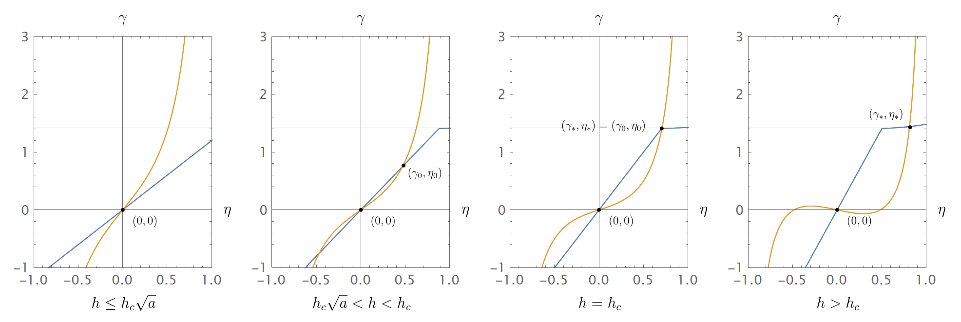
Figure 1: Points $(\gamma,\eta)$ solving the first (blue line) and the second (yellow line) equation of the system (4.15) for pure $3$-spin Hamiltonian.

Lemma 4.3.

If $h^{2}\geq\boldsymbol{\xi}^{\prime\prime}-\boldsymbol{\xi}^{\prime}$ (i.e. $a<1$ or $h\geq h_{c}$) then the point $(\eta_{*},\gamma_{*})$ is the only solution to the system (4.15) (and thus the only critical point of $\widetilde{F}$) in $[\sqrt{2},\infty)\times[0,1)$.

If $h^{2}<\boldsymbol{\xi}^{\prime\prime}-\boldsymbol{\xi}^{\prime}$ (i.e. $a>1$ and $h<h_{c}$) there is no solution to (4.15) in $[\sqrt{2},\infty)\times[0,1)$.

Proof.

We first consider the case $h=0$. Then the calculation reduces to the one for purely random external field carried out in [Fyo15]. Indeed $A=C=0$, and the second equation of (4.15) implies $\gamma=0=\gamma_{*}$. By the first equation, $\eta=\sqrt{{2}/({1-B^{2}})}$ and since

$$1-B^{2}=\frac{4a}{(1+a)^{2}},$$ (4.16)

we have $\sqrt{{2}/({1-B^{2}})}=\eta_{*}$. Therefore, $(\eta_{*},\gamma_{*})$ is the unique solution of (4.15), and the proof is completed in this case.

From now on we assume $h>0$. For $\eta\geq\sqrt{2}$, the first equation of (4.15) implies that $\eta^{2}-2=\left(B\eta-A\gamma\right)^{2}$, which yields the equation

$$(1-B^{2})\eta^{2}+2AB\eta\gamma-(2+A^{2}\gamma^{2})=0.$$

As $B\in(-1,1)$ this is a quadratic equation for $\eta$ with two solutions, only one of which is non-negative since $2(1-B^{2})+A^{2}\gamma^{2}>A^{2}B^{2}\gamma^{2}$, namely

$$\eta=\frac{-AB\gamma+\sqrt{2(1-B^{2})+A^{2}\gamma^{2}}}{1-B^{2}}.$$

We can rewrite this as

$$\eta=\frac{1}{R}\bigg{(}-\frac{B}{A}\gamma+\frac{1}{A}\sqrt{2R+\gamma^{2}}\bigg{)},$$ (4.17)

with

$$R=\frac{1-B^{2}}{A^{2}}\overset{\eqref{eq:Bsquared ident},\eqref{eq:ABC}}{=}\frac{a}{\widetilde{h}^{2}}=\frac{2\boldsymbol{\xi}^{\prime}}{h^{2}}.$$ (4.18)

Plugging this into the second equation of (4.15), we get

$$C\gamma+\frac{A}{R}\left(-\frac{B}{A}\gamma+\frac{1}{A}\sqrt{2R+\gamma^{2}}\right)=\frac{\gamma}{1-\gamma^{2}}.$$

Observing that $\gamma=0$ is not a solution to this equation, after dividing through by $\gamma$ and some simplifications, we obtain

$$CR-B+\sqrt{\frac{2R}{\gamma^{2}}+1}=\frac{R}{1-\gamma^{2}}.$$ (4.19)

By (4.14), $CR-B=1$. Hence, this is equivalent to

$$\sqrt{1+\frac{2R}{\gamma^{2}}}=\frac{R}{1-\gamma^{2}}-1.$$ (4.20)

If one squares both sides to eliminate the square root and multiplies out by $\gamma^{2}(1-\gamma^{2})^{2}$ to remove all fractions, then one gets what is a priori a third degree equation in $\gamma^{2}$. However the third and second degrees cancel yielding the equation $2R(1-2\gamma^{2})=R^{2}\gamma^{2}-2R\gamma^{2}$, which has a single non-negative solution

$$\gamma=\sqrt{\frac{2}{R+2}}\overset{\eqref{eq:R}}{=}\frac{h}{\sqrt{\boldsymbol{\xi}^{\prime}+h^{2}}}\overset{\eqref{eq:etastar}}{=}\gamma_{*}.$$ (4.21)

Plugging this into (4.17) and using that $\sqrt{2R+\gamma_{*}^{2}}=(h^{2}+2\boldsymbol{\xi}^{\prime})/h$ we obtain that $\eta$ must satisfy

$$\eta=\frac{1}{\sqrt{\boldsymbol{\xi}^{\prime}+h^{2}}}\frac{1}{ARh}\left(-Bh^{2}+h^{2}+2\boldsymbol{\xi}^{\prime}\right)=\frac{h^{2}+\boldsymbol{\xi}^{\prime}+\boldsymbol{\xi}^{\prime\prime}}{\sqrt{2\boldsymbol{\xi}^{\prime\prime}(\boldsymbol{\xi}^{\prime}+h^{2})}}\overset{\eqref{eq:etastar}}{=}\eta_{*}.$$ (4.22)

Hence the only possible solution of (4.15) in $[\sqrt{2},\infty)\times[0,1)$ is $(\eta_{*},\gamma_{*})$.

To check that $(\eta_{*},\gamma_{*})$ is indeed a solution (since we squared the equation (4.20) we must verify this), we firstly note that by the definition of $\eta_{*}$

$$\eta_{*}^{2}-2=\frac{(\boldsymbol{\xi}^{\prime}+h^{2}-\boldsymbol{\xi}^{\prime\prime})^{2}}{2\boldsymbol{\xi}^{\prime\prime}(\boldsymbol{\xi}^{\prime}+h^{2})},$$ (4.23)

so that obviously $\eta_{*}\geq 2$. Secondly, by plugging $\eta=\eta_{*}$, $\gamma=\gamma_{*}$ into the second equation of (4.15) we see that these always solve the equation, since

$$C\gamma_{*}+A\eta_{*}=\frac{2\tilde{h}}{(1+a)\boldsymbol{\xi}^{\prime}\sqrt{2\boldsymbol{\xi}^{\prime\prime}(\boldsymbol{\xi}^{\prime}+h^{2})}}(\boldsymbol{\xi}^{\prime\prime}h^{2}+\boldsymbol{\xi}^{\prime}(\boldsymbol{\xi}^{\prime\prime}+\boldsymbol{\xi}^{\prime}+h^{2})),$$ (4.24)

where the last parenthesis factors as $(\boldsymbol{\xi}^{\prime}+h^{2})(\boldsymbol{\xi}^{\prime}+\boldsymbol{\xi}^{\prime\prime})=\boldsymbol{\xi}^{\prime\prime}(\boldsymbol{\xi}^{\prime}+h^{2})(1+a)$, giving

$$C\gamma_{*}+A\eta_{*}=\frac{\tilde{h}\sqrt{2\boldsymbol{\xi}^{\prime\prime}}\sqrt{\boldsymbol{\xi}^{\prime}+h^{2}}}{\boldsymbol{\xi}^{\prime}}=\frac{h\sqrt{\boldsymbol{\xi}^{\prime}+h^{2}}}{\boldsymbol{\xi}^{\prime}}=\frac{\gamma_{*}}{1-\gamma_{*}^{2}}.$$ (4.25)

Lastly, the left-hand side of the first equation of (4.15) equals

$$A\gamma_{*}-B\eta_{*} =\frac{2h^{2}\boldsymbol{\xi}^{\prime\prime}-(\boldsymbol{\xi}^{\prime\prime}-\boldsymbol{\xi}^{\prime})(\boldsymbol{\xi}^{\prime}+\boldsymbol{\xi}^{\prime\prime}+h^{2})}{(\boldsymbol{\xi}^{\prime}+\boldsymbol{\xi}^{\prime\prime})\sqrt{2\boldsymbol{\xi}^{\prime\prime}(\boldsymbol{\xi}^{\prime}+h^{2})}}$$

$$=\frac{2\boldsymbol{\xi}^{\prime\prime}h^{2}-h^{2}(\boldsymbol{\xi}^{\prime\prime}-\boldsymbol{\xi}^{\prime})-(\boldsymbol{\xi}^{\prime\prime}-\boldsymbol{\xi}^{\prime})(\boldsymbol{\xi}^{\prime}+\boldsymbol{\xi}^{\prime\prime})}{\sqrt{2\boldsymbol{\xi}^{\prime\prime}(\boldsymbol{\xi}^{\prime}+h^{2})}(\boldsymbol{\xi}^{\prime}+\boldsymbol{\xi}^{\prime\prime})}$$

$$=\frac{(h^{2}+\boldsymbol{\xi}^{\prime}-\boldsymbol{\xi}^{\prime\prime})(\boldsymbol{\xi}^{\prime}+\boldsymbol{\xi}^{\prime\prime})}{\sqrt{2\boldsymbol{\xi}^{\prime\prime}(\boldsymbol{\xi}^{\prime}+h^{2})}(\boldsymbol{\xi}^{\prime}+\boldsymbol{\xi}^{\prime\prime})}=\frac{h^{2}+\boldsymbol{\xi}^{\prime}-\boldsymbol{\xi}^{\prime\prime}}{\sqrt{2\boldsymbol{\xi}^{\prime\prime}(\boldsymbol{\xi}^{\prime}+h^{2})}}.$$

The right-hand side of the first equation of (4.15) is $\sqrt{\frac{(\boldsymbol{\xi}^{\prime}+h^{2}-\boldsymbol{\xi}^{\prime\prime})^{2}}{2\boldsymbol{\xi}^{\prime\prime}(\boldsymbol{\xi}^{\prime}+h^{2})}}$ by (4.23), which equals the last expression in the above display as long as $h^{2}\geq\boldsymbol{\xi}^{\prime\prime}-\boldsymbol{\xi}^{\prime}$. ∎

We now inspect critical points with $\eta\in[0,\sqrt{2}]$. Recall the definition of $\eta_{0}$, $\gamma_{0}$ from Proposition 4.2.

Lemma 4.4.

$\widetilde{F}$ has at most two critical points in $[0,\sqrt{2}]\times[0,1)$:

If $a<1$ and $h\leq\sqrt{a}h_{c}$ or if $h^{2}>\boldsymbol{\xi}^{\prime\prime}-\boldsymbol{\xi}^{\prime}$ (i.e. $a>1$ or $h>h_{c}$) then the point $(0,0)$ is the only solution to (4.15) in $[0,\sqrt{2}]\times[0,1)$.

If $a<1$ and $h\in(h_{c}\sqrt{a},h_{c}]$, then the points $(0,0)$ and $(\eta_{0},\gamma_{0})$ are the only solutions to (4.15) in $[0,\sqrt{2}]\times[0,1)$.

Proof.

As claimed $\gamma=0,\eta=0$ is always a solution to (4.15). In the remainder of the proof we thus seek to determine when there are other non-negative solutions.

If $\gamma=0$, then $\eta=0$ is the only solution of (4.15) in $[0,\sqrt{2})$, and we can thus assume that $\gamma>0$.

We first consider the case $a=1$ (that is $\boldsymbol{\xi}^{\prime\prime}-\boldsymbol{\xi}^{\prime}=0$) and $h>0$. Then $B=0$ and $A>0$, and the first equation of (4.15) leads to $\gamma=0$, showing that $(0,0)$ is the only solution and completing the proof in this special case.

From now on we can assume $a\neq 1$, and thus $B\neq 0$. Since we consider $\eta\in[0,\sqrt{2}]$ only, the first equation in (4.15) is linear and implies $\eta=\frac{A}{B}\gamma$. If $a>1$, then $A>0$ and $B<0$, and thus there is no solution to (4.15) with $\gamma,\eta>0$. This completes the proof in the case $a>1$. Hence, we assume $a<1$ for the rest of the proof.

Plugging $\eta=\frac{A}{B}\gamma$ into the second equation, we obtain

$$\Big{(}C+\frac{A^{2}}{B}\Big{)}\gamma=\frac{\gamma}{1-\gamma^{2}}.$$

Using the identity $C+\frac{A^{2}}{B}=\frac{h^{2}}{(\boldsymbol{\xi}^{\prime\prime}-\boldsymbol{\xi}^{\prime})a}$ which follows from (4.14), it is easy to see that any non-zero solution satisfies

$$\gamma^{2}=1-\frac{(\boldsymbol{\xi}^{\prime\prime}-\boldsymbol{\xi}^{\prime})a}{h^{2}}.$$ (4.26)

If $h\leq h_{c}\sqrt{a}$ then the right-hand side is non-positive, so that there are no non-zero solutions to (4.26) and thus no further solutions to (4.15). This completes the proof of the case $a<1$ and $h\leq h_{c}\sqrt{a}$. When $h>h_{c}\sqrt{a}$ then (4.26) has unique positive solution

$$\sqrt{1-\frac{(\boldsymbol{\xi}^{\prime\prime}-\boldsymbol{\xi}^{\prime})a}{h^{2}}}\overset{\eqref{eq:defhtildea},\eqref{eq:eta0}}{=}\gamma_{0}.$$ (4.27)

The matching $\eta$, computed from the first equation, is given by $\eta=\frac{A}{B}\gamma_{0}=\eta_{0}$ (see (4.14)), for $\eta_{0}$ as claimed in (4.9). Thus $(\eta_{0},\gamma_{0})$ is the only possible solution to (4.15) in $[0,\sqrt{2}]\times[0,1)$ other than $(0,0)$, and is a solution if indeed $\eta_{0}\leq\sqrt{2}$.

If $h\leq h_{c}$, then $\eta_{0}\leq\sqrt{2}$ holds true, because $\eta_{0}$ is an increasing functions of $h$ by (4.27) and (4.9), and $\eta_{0}=\sqrt{2}$ for $h=h_{c}$, by (4.9). This completes the proof of the case $a<1,h\in(\sqrt{a}h_{c},h_{c}]$.

Otherwise, if $h>h_{c}$, then $\eta_{0}>\sqrt{2}$, so $(\eta_{0},\gamma_{0})$ is not a solution to (4.15). This completes the proof of the case $a<1,h>h_{c}$. ∎

We now have all ingredients to complete the proof of Proposition 4.2.

Proof of (iii).

The claim (iii) follows directly from the previous two lemmas, as $(0,0)$ is the only critical point for $h\leq h_{c}\sqrt{a}$, so it must be a maximum. ∎

For claims (i), (ii) we need to evaluate $\widetilde{F}$ at the remaining critical points and show that it is positive there.

Proof of (i).

By Lemmas 4.3, 4.4, and (4.13) the possible maximizers of $\tilde{F}$ are $(0,0)$ and $\pm(\eta_{*},\gamma_{*})$. We need to compute $\widetilde{F}(\eta_{*},\gamma_{*})$ and show that it is positive. To this end we write

$$\eta_{*}=\frac{1}{\sqrt{2}}\Big{(}z+\frac{1}{z}\Big{)}\quad\text{for }z=\sqrt{\frac{\boldsymbol{\xi}^{\prime\prime}}{h^{2}+\boldsymbol{\xi}^{\prime}}}.$$ (4.28)

If $x=\frac{1}{\sqrt{2}}(z+\frac{1}{z})$ for $0<z<1$, then the identity

$$\frac{x^{2}}{2}+\Phi(x)=\frac{1}{2}+\frac{z^{2}}{2}-\ln z$$ (4.29)

can be proved from the definition (2.7) of $\Phi$ by noting that $\sqrt{x^{2}-2}=\frac{1}{\sqrt{2}}(\frac{1}{z}-z)$. In addition, by (4.7),

$$\frac{1}{2}\ln\big{(}1-\gamma_{*}^{2}\big{)}=\frac{1}{2}\ln\bigg{(}\frac{\boldsymbol{\xi}^{\prime\prime}}{\boldsymbol{\xi}^{\prime}+h^{2}}\bigg{)}.$$

Inserting the last two displays into (4.6) and cancelling the terms containing the logarithm, we obtain

$$\widetilde{F}(\eta_{*},\gamma_{*})=\frac{\widetilde{h}^{2}\gamma_{*}^{2}}{a}-\frac{(\eta_{*}-\widetilde{h}\gamma_{*})^{2}}{1+a}+\frac{1}{2}+\frac{1}{2}\frac{\boldsymbol{\xi}^{\prime\prime}}{h^{2}+\boldsymbol{\xi}^{\prime}}-\frac{1}{2}\ln\bigg{(}\frac{\boldsymbol{\xi}^{\prime\prime}}{\boldsymbol{\xi}^{\prime}}\bigg{)}.$$ (4.30)

Plugging in all definitions (see (4.5) and (4.7)) and using $\frac{\widetilde{h}^{2}\gamma_{*}^{2}}{a}=\frac{h^{4}}{2\boldsymbol{\xi}^{\prime}\left(\boldsymbol{\xi}^{\prime}+h^{2}\right)}$ and $\frac{(\eta_{*}-\widetilde{h}\gamma_{*})^{2}}{1+a}=\frac{1}{2}\frac{\boldsymbol{\xi}^{\prime}+\boldsymbol{\xi}^{\prime\prime}}{\boldsymbol{\xi}^{\prime}+h^{2}}$ one verifies (4.8).

Applying the elementary inequality

$$\ln y\leq y-1\text{ for all }y>0\quad\text{ (with equality only if }y=1).$$ (4.31)

with $y=\frac{\boldsymbol{\xi}^{\prime\prime}}{\boldsymbol{\xi}^{\prime}}$ to (4.8) we get for $h^{2}>\boldsymbol{\xi}^{\prime\prime}-\boldsymbol{\xi}^{\prime}$ that

$$\widetilde{F}(\eta_{*},\gamma_{*})>\frac{\boldsymbol{\xi}^{\prime\prime}-\boldsymbol{\xi}^{\prime}}{2\boldsymbol{\xi}^{\prime}}-\frac{1}{2}\Big{(}\frac{\boldsymbol{\xi}^{\prime\prime}}{\boldsymbol{\xi}^{\prime}}-1\Big{)}=0=\widetilde{F}(0,0).$$ (4.32)

Thus $\pm(\eta_{*},\gamma_{*})$ are the unique maximizers of $\tilde{F}$ if $h^{2}>\boldsymbol{\xi}^{\prime\prime}-\boldsymbol{\xi}^{\prime}$. This proves claim (i) of the proposition. ∎

Proof of (ii).

By Lemmas 4.3, 4.4 and (4.13), we have that $\pm(\eta_{0},\gamma_{0})$ are the only possible maximizers of $\tilde{F}$ for $h\in(h_{c}\sqrt{a},h_{c})$. When $a<1$ and $h=h_{c}$, then $\eta_{*}=\eta_{0}=\sqrt{2}$, $x_{*}=x_{0}$ and $\gamma_{*}=\gamma_{0}$, so this holds also for $h=h_{c}$. Thus to verify (ii) we must compute $F(x_{0},\gamma_{0})$. To this end we use that $\Phi(\eta_{0})=0$ since $|\eta_{0}|\leq\sqrt{2}$. Plugging (4.9) into the (4.6) and using that $1-\gamma_{0}^{2}=\frac{1}{H}$ we obtain

$$\frac{\widetilde{h}^{2}\gamma_{0}^{2}}{a}-\frac{(\eta_{0}-\widetilde{h}\gamma_{0})^{2}}{1+a}+\frac{\eta_{0}^{2}}{2}$$

$$=\gamma_{0}^{2}\left(\frac{h^{2}}{2\boldsymbol{\xi}^{\prime\prime}a}-\frac{1}{1+a}{\bigg{(}\frac{h\sqrt{2\boldsymbol{\xi}^{\prime\prime}}}{\boldsymbol{\xi}^{\prime\prime}-\boldsymbol{\xi}^{\prime}}-\frac{h}{\sqrt{2\boldsymbol{\xi}^{\prime\prime}}}\bigg{)}^{2}}+\frac{2h^{2}\boldsymbol{\xi}^{\prime\prime}}{2(\boldsymbol{\xi}^{\prime\prime}-\boldsymbol{\xi}^{\prime})^{2}}\right)$$

$$=\left(1-\frac{1}{H}\right)\left(\frac{h^{2}}{2\boldsymbol{\xi}^{\prime}}-\frac{h^{2}}{\boldsymbol{\xi}^{\prime\prime}+\boldsymbol{\xi}^{\prime}}\bigg{(}{\frac{2\boldsymbol{\xi}^{\prime\prime 2}}{(\boldsymbol{\xi}^{\prime\prime}-\boldsymbol{\xi}^{\prime})^{2}}-2\frac{\boldsymbol{\xi}^{\prime\prime}}{\boldsymbol{\xi}^{\prime\prime}-\boldsymbol{\xi}^{\prime}}}+\frac{1}{2}\bigg{)}+\frac{2h^{2}\boldsymbol{\xi}^{\prime\prime}}{2(\boldsymbol{\xi}^{\prime\prime}-\boldsymbol{\xi}^{\prime})^{2}}\right)$$

$$=\left(1-\frac{1}{H}\right)\left(\frac{h^{2}}{2\boldsymbol{\xi}^{\prime}}+\frac{h^{2}}{2}\frac{\left(\boldsymbol{\xi}^{\prime\prime}\right)^{2}-\left(\boldsymbol{\xi}^{\prime}\right)^{2}}{\left(\boldsymbol{\xi}^{\prime\prime}-\boldsymbol{\xi}^{\prime}\right)^{2}\left(\boldsymbol{\xi}^{\prime\prime}+\boldsymbol{\xi}^{\prime}\right)}\right)$$

$$=\left(1-\frac{1}{H}\right)\left(\frac{h^{2}}{2\boldsymbol{\xi}^{\prime}}+\frac{h^{2}}{2(\boldsymbol{\xi}^{\prime\prime}-\boldsymbol{\xi}^{\prime})}\right)=\left(1-\frac{1}{H}\right)\frac{H}{2}=\frac{H-1}{2}.$$

This gives (4.10). As $H>1$ for $h>\sqrt{a}h_{c}$ and $a<1$, we see immediately using (4.31) that $\widetilde{F}(\eta_{0},\gamma_{0})>0=\widetilde{F}(0,0)$. This proves the claim (ii).

∎

Proof of (iv).

Substituting $\boldsymbol{\xi}^{\prime\prime}=\boldsymbol{\xi}^{\prime}$ and $h=0$ into $F$ and $\tilde{F}$, it is straightforward to check $F(x,\gamma)=\tilde{F}(\eta,\gamma)=\frac{1}{2}\ln{(1-\gamma^{2})}+\Phi(\eta).$ By (4.12), $\Phi(\eta)\leq 0$ for any $\eta\in{\mathbb{R}}$. Hence, since $\ln{(1-\gamma^{2})}\leq 0$, the maxima of $F$ and $\tilde{F}$ are $0$. ∎

This completes the proof of all parts of Proposition 4.2. ∎

Having control over the exponential term we are prepared to finish this section with the proof of claim (1.12) which gives the annealed complexity in the nontrivial regime.

Proof of Theorem 1.2(ii).

By Proposition 3.1 with $R=E=\mathbb{R}$ and $\Gamma=[-1,1]$,

$$\mathbb{E}[\mathcal{N}_{N}]=\exp\left(N\left[-\frac{h^{2}}{2\boldsymbol{\xi}^{\prime}}+\frac{1}{2}\ln\left(\frac{\boldsymbol{\xi}^{\prime\prime}}{\boldsymbol{\xi}^{\prime}}\right)\right]+o(N)\right)\int_{-1}^{1}\int_{-\infty}^{\infty}\frac{e^{NG(x,\gamma)}}{(1-\gamma)^{3/2}}\,\rho_{N}\left(\frac{x+h\gamma}{\sqrt{2\boldsymbol{\xi}^{\prime\prime}}}\right)\,\mathrm{d}x\,\mathrm{d}\gamma,$$

which by Lemma 4.1 equals

$$\exp\left(N\left[-\frac{h^{2}}{2\boldsymbol{\xi}^{\prime}}+\frac{1}{2}\ln\left(\frac{\boldsymbol{\xi}^{\prime\prime}}{\boldsymbol{\xi}^{\prime}}\right)\right]+o(N)\right)\int_{-1}^{1}\int_{-\infty}^{\infty}e^{NF(x,\gamma)(1+o(1))}\,\,\mathrm{d}x\,\mathrm{d}\gamma.$$

Bounding the integral over the complement of a sufficiently large box around the origin from above using (4.2) gives an upper bound of $e^{-LN}$ for any $L$. Hence restricting to a bounded region only causes vanishing multiplicative error and then the Laplace method yields

$$\mathbb{E}\left[\mathcal{N}_{N}\right]=\exp\left(N\left[\frac{1}{2}\ln\left(\frac{\boldsymbol{\xi}^{\prime\prime}}{\boldsymbol{\xi}^{\prime}}\right)-\frac{h^{2}}{2\boldsymbol{\xi}^{\prime}}+\max_{\gamma\in[-1,1],x\in\mathbb{R}}F(x,\gamma)\right]+o(N)\right).$$ (4.33)

Applying Proposition 4.2(ii, iii, iv) then implies the claim (1.12). ∎

Note that by the same argument using (4.8) of Proposition 4.2(i) we obtain

$$\lim_{N\to\infty}\frac{1}{N}\ln\mathbb{E}\left[\mathcal{N}_{N}\right]=0\quad\text{if }h^{2}>\boldsymbol{\xi}^{\prime\prime}-\boldsymbol{\xi}^{\prime},$$ (4.34)

which is a weaker form of the triviality claimed in (1.11).

5 Exact asymptotic in the trivial regime

In this section we consider the trivial regime $h^{2}>\boldsymbol{\xi}^{\prime\prime}-\boldsymbol{\xi}^{\prime}$, and conclude the proof of the asymptotic complexity (1.11).

Proof of Theorem 1.2(i).

By Proposition 3.1, using $E=R=\mathbb{R}$ and $\Gamma=[-1,1]$, we have

$$\mathbb{E}[\mathcal{N}_{N}]=e^{-\frac{Nh^{2}}{2\boldsymbol{\xi}^{\prime}}}\left(\frac{\boldsymbol{\xi}^{\prime\prime}}{\boldsymbol{\xi}^{\prime}}\right)^{\frac{N-1}{2}}\,\frac{2N}{\sqrt{\pi(\boldsymbol{\xi}^{\prime}+\boldsymbol{\xi}^{\prime\prime})}}\,\frac{\Gamma(\frac{N}{2})}{\Gamma(\frac{N-1}{2})}\int_{\mathbb{R}}\int_{[-1,1]}\frac{e^{NG(x,\gamma)}}{(1-\gamma^{2})^{{3}/{2}}}\rho_{N}\left(\frac{x+h\gamma}{\sqrt{2\boldsymbol{\xi}^{\prime\prime}}}\right)\,\mathrm{d}\gamma\,\mathrm{d}x.$$

Following the argument of the proof of Theorem 1.2(ii) and using (4.2) we can bound the integral outside a sufficiently large box above by $e^{-LN}$ for any $L$. Hence removing the complement of a sufficiently large box only causes vanishing error. By Laplace principle we then may further restrict to any fixed neighborhood $[x_{*}-\varepsilon,x_{*}+\varepsilon]\times[\gamma_{*}-\varepsilon,\gamma_{*}+\varepsilon]$ of the maximizers of the exponential contribution, still causing only vanishing error. Since we assume that $h^{2}>\boldsymbol{\xi}^{\prime\prime}-\boldsymbol{\xi}^{\prime}$, it follows from Proposition 4.2(i) that these maximizers are $\gamma_{*}$ and $x_{*}$, and in addition $\frac{x_{*}+h\gamma_{*}}{\sqrt{2\boldsymbol{\xi}^{\prime\prime}}}=\eta_{*}>\sqrt{2}$ by (4.23). Hence choosing $\varepsilon>0$ small enough allows the use of Lemma 2.2(i). Recalling the definition of $\eta$ from (4.4), we obtain that $\mathbb{E}[\mathcal{N}_{N}]$ equals

$$e^{-\frac{Nh^{2}}{2\boldsymbol{\xi}^{\prime}}}\left(\frac{\boldsymbol{\xi}^{\prime\prime}}{\boldsymbol{\xi}^{\prime}}\right)^{\frac{N-1}{2}}\frac{2\sqrt{N}}{\pi\sqrt{(\boldsymbol{\xi}^{\prime}+\boldsymbol{\xi}^{\prime\prime})}}\,\frac{\Gamma(\frac{N}{2})}{\Gamma(\frac{N-1}{2})}\int_{x_{*}-\varepsilon}^{x_{*}+\varepsilon}\int_{\gamma_{*}-\varepsilon}^{\gamma_{*}+\varepsilon}\frac{(1-\gamma^{2})^{-\frac{3}{2}}e^{NF(x,\gamma)}}{(\eta^{2}-2)^{\frac{1}{4}}\,(|\eta|+\sqrt{\eta^{2}-2})^{\frac{1}{2}}}\,\mathrm{d}\gamma\,\mathrm{d}x+o(1).$$

Note that an extra factor $2$ arises since the neighborhood of $(-\gamma_{*},-x_{*})$ by symmetry has the same contribution as the neighborhood of $(\gamma_{*},x_{*})$. Using the Laplace principle with second order corrections we obtain that the above is

$$e^{-\frac{Nh^{2}}{2\boldsymbol{\xi}^{\prime}}}\left(\frac{\boldsymbol{\xi}^{\prime\prime}}{\boldsymbol{\xi}^{\prime}}\right)^{\frac{N-1}{2}}\frac{2\sqrt{N}}{\pi\sqrt{(\boldsymbol{\xi}^{\prime}+\boldsymbol{\xi}^{\prime\prime})}}\,\frac{\Gamma(\frac{N}{2})}{\Gamma(\frac{N-1}{2})}\frac{(1-\gamma_{*}^{2})^{-\frac{3}{2}}e^{NF(x_{*},\gamma_{*})}}{(\eta_{*}^{2}-2)^{\frac{1}{4}}\,(|\eta_{*}|+\sqrt{\eta_{*}^{2}-2})^{\frac{1}{2}}}\frac{2\pi}{N\sqrt{|\operatorname{det}\nabla^{2}F(x_{*},\gamma_{*})|}}+o(1).$$

Using that ${\Gamma(\frac{N}{2})}/{\Gamma(\frac{N-1}{2})}\sim\sqrt{N/2}$ and plugging in the value of $F(x_{*},\gamma_{*})$ from (4.8) of Proposition 4.2(i), we benefit from cancellations and obtain

$$\mathbb{E}[\mathcal{N}_{N}]=\frac{2\sqrt{2}\sqrt{\boldsymbol{\xi}^{\prime}}(1-\gamma_{*}^{2})^{-\frac{3}{2}}}{\sqrt{\boldsymbol{\xi}^{\prime\prime}}\sqrt{(\boldsymbol{\xi}^{\prime}+\boldsymbol{\xi}^{\prime\prime})}(\eta_{*}^{2}-2)^{\frac{1}{4}}\,(|\eta_{*}|+\sqrt{\eta_{*}^{2}-2})^{\frac{1}{2}}\sqrt{|\operatorname{det}\nabla^{2}F(x_{*},\gamma_{*})|}}+o(1).$$ (5.1)

Calculating the second order derivatives of $F$ from (4.1), we obtain:

$$\partial^{2}_{x}F(x,\gamma) =\frac{1}{2\boldsymbol{\xi}^{\prime\prime}}\left(\frac{\boldsymbol{\xi}^{\prime}-\boldsymbol{\xi}^{\prime\prime}}{\boldsymbol{\xi}^{\prime}+\boldsymbol{\xi}^{\prime\prime}}+\Phi^{\prime\prime}(\eta)\right),$$

$$\partial^{2}_{\gamma}F(x,\gamma) =-\frac{1+\gamma^{2}}{(1-\gamma^{2})^{2}}+\frac{h^{2}}{2\boldsymbol{\xi}^{\prime\prime}}\left(1+2\frac{\boldsymbol{\xi}^{\prime\prime}}{\boldsymbol{\xi}^{\prime}}+\Phi^{\prime\prime}(\eta)\right)$$

$$=\frac{h^{2}}{2\boldsymbol{\xi}^{\prime\prime}}\left(-\frac{2\boldsymbol{\xi}^{\prime\prime}(\boldsymbol{\xi}^{\prime}+h^{2})(\boldsymbol{\xi}^{\prime}+2h^{2})}{h^{2}(\boldsymbol{\xi}^{\prime})^{2}}+1+2\frac{\boldsymbol{\xi}^{\prime\prime}}{\boldsymbol{\xi}^{\prime}}+\Phi^{\prime\prime}(\eta)\right),$$ (5.2)

$$\partial_{x}\partial_{\gamma}F(x,\gamma) =\frac{h}{2\boldsymbol{\xi}^{\prime\prime}}\left(1+\Phi^{\prime\prime}(\eta)\right).$$

We now plug in $\gamma=\gamma^{*}$ and $x=x_{*}$, so that $\eta=\eta_{*}$ (recall the formulas from (4.7)). Using $\Phi^{\prime\prime}(\eta)=-\frac{\eta}{\sqrt{\eta^{2}-2}}$ for $\eta>\sqrt{2}$ and $\sqrt{\eta_{*}^{2}-2}=\frac{\boldsymbol{\xi}^{\prime}+h^{2}-\boldsymbol{\xi}^{\prime\prime}}{\sqrt{2\boldsymbol{\xi}^{\prime\prime}(\boldsymbol{\xi}^{\prime}+h^{2})}}$(recall (4.23)), one verifies that $\Phi^{\prime\prime}(\eta_{*})=-\frac{\boldsymbol{\xi}^{\prime}+h^{2}+\boldsymbol{\xi}^{\prime\prime}}{\boldsymbol{\xi}^{\prime}+h^{2}-\boldsymbol{\xi}^{\prime\prime}}$. Using also $\gamma_{*}^{2}=\frac{h^{2}}{\boldsymbol{\xi}^{\prime}+h^{2}}$ and simplifying one obtains

$$\partial^{2}_{x}F(x_{*},\gamma_{*}) =-\frac{2\boldsymbol{\xi}^{\prime}+h^{2}}{\left(h^{2}+\boldsymbol{\xi}^{\prime}-\boldsymbol{\xi}^{\prime\prime}\right)\left(\boldsymbol{\xi}^{\prime}+\boldsymbol{\xi}^{\prime\prime}\right)},$$

$$\partial^{2}_{\gamma}F(x_{*},\gamma_{*}) =-\frac{\left(\boldsymbol{\xi}^{\prime}+2h^{2}\right)\left(\boldsymbol{\xi}^{\prime}+h^{2}\right)}{\left(\boldsymbol{\xi}^{\prime}\right)^{2}}+h^{2}\frac{h^{2}-\boldsymbol{\xi}^{\prime\prime}}{\boldsymbol{\xi}^{\prime}\left(h^{2}+\boldsymbol{\xi}^{\prime}-\boldsymbol{\xi}^{\prime\prime}\right)},$$

$$\partial_{x}\partial_{\gamma}F(x_{*},\gamma_{*}) =-\frac{h}{h^{2}+\boldsymbol{\xi}^{\prime}-\boldsymbol{\xi}^{\prime\prime}}.$$

Using these expressions in the formula for the determinant of a $2\times 2$ matrix and extracting factors $h^{2}+\boldsymbol{\xi}^{\prime}-\boldsymbol{\xi}^{\prime\prime}$, $(\boldsymbol{\xi}^{\prime})^{2}$ and $\boldsymbol{\xi}^{\prime}+\boldsymbol{\xi}^{\prime\prime}$ one obtains that $\operatorname{det}\nabla^{2}F(x_{*},\gamma_{*})$ equals

$$\begin{split}&\frac{1}{h^{2}+\boldsymbol{\xi}^{\prime}-\boldsymbol{\xi}^{\prime\prime}}\left(\frac{2\boldsymbol{\xi}^{\prime}+h^{2}}{\boldsymbol{\xi}^{\prime}+\boldsymbol{\xi}^{\prime\prime}}\left(\frac{\left(\boldsymbol{\xi}^{\prime}+2h^{2}\right)\left(\boldsymbol{\xi}^{\prime}+h^{2}\right)}{\left(\boldsymbol{\xi}^{\prime}\right)^{2}}-\frac{h^{2}(h^{2}-\boldsymbol{\xi}^{\prime\prime})}{\boldsymbol{\xi}^{\prime}\left(h^{2}+\boldsymbol{\xi}^{\prime}-\boldsymbol{\xi}^{\prime\prime}\right)}\right)-\frac{h^{2}}{h^{2}+\boldsymbol{\xi}^{\prime}-\boldsymbol{\xi}^{\prime\prime}}\right)\\ &=\frac{1}{\left(h^{2}+\boldsymbol{\xi}^{\prime}-\boldsymbol{\xi}^{\prime\prime}\right)\left(\boldsymbol{\xi}^{\prime}\right)^{2}\left(\boldsymbol{\xi}^{\prime}+\boldsymbol{\xi}^{\prime\prime}\right)}\bigg{(}\left(2\boldsymbol{\xi}^{\prime}+h^{2}\right)\left(\boldsymbol{\xi}^{\prime}+2h^{2}\right)\left(\boldsymbol{\xi}^{\prime}+h^{2}\right)\\ &\quad-\frac{h^{2}\left(h^{2}-\boldsymbol{\xi}^{\prime\prime}\right)\boldsymbol{\xi}^{\prime}}{h^{2}+\boldsymbol{\xi}^{\prime}-\boldsymbol{\xi}^{\prime\prime}}\left(2\boldsymbol{\xi}^{\prime}+h^{2}\right)-\frac{h^{2}\left(\boldsymbol{\xi}^{\prime}\right)^{2}\left(\boldsymbol{\xi}^{\prime}+\boldsymbol{\xi}^{\prime\prime}\right)}{h^{2}+\boldsymbol{\xi}^{\prime}-\boldsymbol{\xi}^{\prime\prime}}\bigg{)}.\end{split}$$ (5.3)

The last two terms equal

$$h^{2}\frac{\left(h^{2}-\boldsymbol{\xi}^{\prime\prime}\right)\boldsymbol{\xi}^{\prime}}{h^{2}+\boldsymbol{\xi}^{\prime}-\boldsymbol{\xi}^{\prime\prime}}\left(2\boldsymbol{\xi}^{\prime}+h^{2}\right)+\frac{h^{2}\left(\boldsymbol{\xi}^{\prime}\right)^{2}\left(\boldsymbol{\xi}^{\prime}+\boldsymbol{\xi}^{\prime\prime}\right)}{h^{2}+\boldsymbol{\xi}^{\prime}-\boldsymbol{\xi}^{\prime\prime}}=\frac{h^{2}\left(h^{2}-\boldsymbol{\xi}^{\prime\prime}\right)\boldsymbol{\xi}^{\prime}\left(2\boldsymbol{\xi}^{\prime}+h^{2}\right)+h^{2}\left(\boldsymbol{\xi}^{\prime}\right)^{2}\left(\boldsymbol{\xi}^{\prime}+\boldsymbol{\xi}^{\prime\prime}\right)}{h^{2}+\boldsymbol{\xi}^{\prime}-\boldsymbol{\xi}^{\prime\prime}}.$$

Remarkably a factor of $h^{2}+\boldsymbol{\xi}^{\prime}-\boldsymbol{\xi}^{\prime\prime}$ can be pulled out of the numerator by writing

$$\begin{array}[]{l}h^{2}\left(h^{2}-\boldsymbol{\xi}^{\prime\prime}\right)\boldsymbol{\xi}^{\prime}\left(2\boldsymbol{\xi}^{\prime}+h^{2}\right)+h^{2}\left(\boldsymbol{\xi}^{\prime}\right)^{2}\left(\boldsymbol{\xi}^{\prime}+\boldsymbol{\xi}^{\prime\prime}\right)\\ =h^{2}\left(h^{2}+\boldsymbol{\xi}^{\prime}-\boldsymbol{\xi}^{\prime\prime}\right)\boldsymbol{\xi}^{\prime}\left(2\boldsymbol{\xi}^{\prime}+h^{2}\right)-h^{2}\left(\boldsymbol{\xi}^{\prime}\right)^{2}\left(2\boldsymbol{\xi}^{\prime}+h^{2}\right)+h^{2}\left(\boldsymbol{\xi}^{\prime}\right)^{2}\left(\boldsymbol{\xi}^{\prime}+\boldsymbol{\xi}^{\prime\prime}\right)\\ =h^{2}\left(h^{2}+\boldsymbol{\xi}^{\prime}-\boldsymbol{\xi}^{\prime\prime}\right)\boldsymbol{\xi}^{\prime}\left(2\boldsymbol{\xi}^{\prime}+h^{2}\right)-h^{2}\left(\boldsymbol{\xi}^{\prime}\right)^{2}\left(\boldsymbol{\xi}^{\prime}+h^{2}-\boldsymbol{\xi}^{\prime\prime}\right)\\ =(h^{2}+\boldsymbol{\xi}^{\prime}-\boldsymbol{\xi}^{\prime\prime})\left(h^{2}+\boldsymbol{\xi}^{\prime}\right)h^{2}\boldsymbol{\xi}^{\prime}.\end{array}$$ (5.4)

Thus the determinant (5.3) becomes

$$\frac{\left(\boldsymbol{\xi}^{\prime}+h^{2}\right)\left\{\left(2\boldsymbol{\xi}^{\prime}+h^{2}\right)\left(\boldsymbol{\xi}^{\prime}+2h^{2}\right)-h^{2}\boldsymbol{\xi}^{\prime}\right\}}{\left(h^{2}+\boldsymbol{\xi}^{\prime}-\boldsymbol{\xi}^{\prime\prime}\right)\left(\boldsymbol{\xi}^{\prime}\right)^{2}\left(\boldsymbol{\xi}^{\prime}+\boldsymbol{\xi}^{\prime\prime}\right)}.$$ (5.5)

By multiplying out and completing the square the second term of the numerator simplifies to $2(\boldsymbol{\xi}^{\prime}+h^{2})^{2}$ and we obtain

$$\operatorname{det}\nabla^{2}F(x_{*},\gamma_{*})=\frac{2\left(\boldsymbol{\xi}^{\prime}+h^{2}\right)^{3}}{\left(h^{2}+\boldsymbol{\xi}^{\prime}-\boldsymbol{\xi}^{\prime\prime}\right)\left(\boldsymbol{\xi}^{\prime}\right)^{2}\left(\boldsymbol{\xi}^{\prime}+\boldsymbol{\xi}^{\prime\prime}\right)}.$$ (5.6)

Using (4.7), $\eta_{*}=\frac{1}{\sqrt{2}}(\frac{1}{z}+z)$ and $\sqrt{\eta_{*}^{2}-2}=\frac{1}{\sqrt{2}}(\frac{1}{z}-z)$ with $z=\sqrt{\frac{\boldsymbol{\xi}^{\prime\prime}}{\boldsymbol{\xi}^{\prime}+h^{2}}}\leq 1$ (recall (4.28)), the remaining terms simplify to

$$(1-\gamma_{*}^{2})^{-{3}/{2}}=\boldsymbol{\xi}^{\prime-3/2}\,(\boldsymbol{\xi}^{\prime}+h^{2})^{3/2},$$ (5.7)

$$\frac{1}{(\eta_{*}^{2}-2)^{1/4}(|\eta_{*}|+\sqrt{\eta_{*}^{2}-2})^{1/2}}=\sqrt{\frac{\boldsymbol{\xi}^{\prime\prime}}{\boldsymbol{\xi}^{\prime}+h^{2}-\boldsymbol{\xi}^{\prime\prime}}}.$$ (5.8)

Plugging (5.6)–(5.8) into (5.1) we obtain $\mathbb{E}[\mathcal{N}_{N}]\sim 2$, which completes the proof of (1.11). ∎

6 Characterization of maximum

In the final section of this paper we prove the asypmtotic equalities (1.5)–(1.8) describing the properties of the field at its maximizer. The proofs are based on the following two lemmas.

Lemma 6.1.

If there exists $p\geq 2$ such that $\xi(s)=a_{p}s^{p}$, then $p_{x,\gamma}(E)=\boldsymbol{1}_{E}\big{(}\frac{x\boldsymbol{\xi}^{\prime}}{\boldsymbol{\xi}^{\prime}+\boldsymbol{\xi}^{\prime\prime}}+h\gamma\big{)}$. Otherwise, for $x\in{\mathbb{R}}$ and $E\subset{\mathbb{R}}$,

$$p_{x,\gamma}(E)=\frac{1}{\sqrt{2\pi}J}\int_{E}\exp\bigg{(}-\frac{N}{2J^{2}}\bigg{(}y-\bigg{(}\frac{\boldsymbol{\xi}^{\prime}}{\boldsymbol{\xi}^{\prime}+\boldsymbol{\xi}^{\prime\prime}}x+h\gamma\bigg{)}\bigg{)}^{2}\bigg{)}\,\mathrm{d}y,$$ (6.1)

where $J^{2}=\frac{\boldsymbol{\xi}(\boldsymbol{\xi}^{\prime}+\boldsymbol{\xi}^{\prime\prime})-\boldsymbol{\xi}^{\prime 2}}{\boldsymbol{\xi}^{\prime}+\boldsymbol{\xi}^{\prime\prime}}$ is a positive number.

Proof.

Using Lemma B.1,

$$\mathbb{E}\partial_{r}H_{N}(\sigma)^{2}=N(\boldsymbol{\xi}^{\prime}+\boldsymbol{\xi}^{\prime\prime}),\quad\mathbb{E}H_{N}(\sigma)^{2}=N\boldsymbol{\xi},\quad\mathbb{E}\partial_{r}H_{N}(\sigma)H_{N}(\sigma)=N\boldsymbol{\xi}^{\prime}.$$ (6.2)

Using standard Gaussian conditioning formulas, this implies that, conditionally on $\partial_{r}H_{N}(\sigma)$, $H_{N}(\sigma)$ is a Gaussian random variable with mean $\frac{\boldsymbol{\xi}^{\prime}}{\boldsymbol{\xi}^{\prime}+\boldsymbol{\xi}^{\prime\prime}}\partial_{r}H_{N}(\sigma)$ and variance $NJ^{2}$. By Jensen’s inequality we have

$$\begin{split}\boldsymbol{\xi}^{\prime}+\boldsymbol{\xi}^{\prime\prime}&=\sum_{p\geq 1}p^{2}a_{p}=\left(\sum_{p\geq 1}a_{p}\right)\frac{\sum_{p\geq 1}p^{2}a_{p}}{\sum_{p\geq 1}a_{p}}\\ &\geq\left(\sum_{p\geq 1}a_{p}\right)\left(\frac{\sum_{p\geq 1}pa_{p}}{\sum_{p\geq 1}a_{p}}\right)^{2}=\frac{(\boldsymbol{\xi}^{\prime})^{2}}{\boldsymbol{\xi}},\end{split}$$

with equality only if $\xi(s)=a_{p}s^{p}$ for some $p\geq 2$. It follows that if $\xi$ takes this form, then $J=0$, and otherwise $J>0$. If $J=0$, then $H_{N}(\sigma)=\frac{\boldsymbol{\xi}^{\prime}}{\boldsymbol{\xi}^{\prime}+\boldsymbol{\xi}^{\prime\prime}}\partial_{r}H_{N}(\sigma)$ almost surely, and thus $p_{x,\gamma}(E)=\boldsymbol{1}_{E}(\frac{x\boldsymbol{\xi}^{\prime}}{\boldsymbol{\xi}^{\prime}+\boldsymbol{\xi}^{\prime\prime}}+h\gamma)$. If $J^{2}>0$, we obtain (6.1) as claimed. ∎

Lemma 6.2.

Assume that $h^{2}>\boldsymbol{\xi}^{\prime\prime}-\boldsymbol{\xi}^{\prime}$. Recall $x_{*}$ and $\gamma_{*}$ from (4.7) and set $y_{*}=\sqrt{\boldsymbol{\xi}^{\prime}+h^{2}}$. Then for all closed sets $\Gamma\subset[-1,1]$ and $R,E\subset{\mathbb{R}}$ with $\pm(\gamma_{*},x_{*},y_{*})\notin\Gamma\times R\times E$, we have $\lim_{N\to\infty}\mathbb{E}[\mathcal{N}_{N}(\Gamma,R,E)]=0$.

Proof.

We first assume that $\xi(s)$ is not of the form $a_{p}s^{p}$. By Proposition 3.1, Lemmas 6.1 and 4.1,

$$\begin{split}&\mathbb{E}\big{[}|\mathcal{N}_{N}(\Gamma,R,E)|\big{]}\\ &=\exp{\left(N\left(\frac{1}{2}\ln{\left(\frac{\boldsymbol{\xi}^{\prime\prime}}{\boldsymbol{\xi}^{\prime}}\right)}-\frac{h^{2}}{2\boldsymbol{\xi}^{\prime}}+o(1)\right)\right)}\int_{R}\int_{\Gamma}\frac{e^{NG(x,\gamma)}}{(1-\gamma^{2})^{\frac{3}{2}}}\rho_{N}\left(\frac{x+h\gamma}{\sqrt{2\boldsymbol{\xi}^{\prime\prime}}}\right)p_{x,\gamma}(E)\,\mathrm{d}\gamma\,\mathrm{d}x\\ &\leq\exp{\left(N\left(\frac{1}{2}\ln{\left(\frac{\boldsymbol{\xi}^{\prime\prime}}{\boldsymbol{\xi}^{\prime}}\right)}-\frac{h^{2}}{2\boldsymbol{\xi}^{\prime}}+o(1)\right)\right)}\\ &\quad\times\int_{E}\int_{R}\int_{\Gamma}\exp{\left(N\left(F(x,\gamma)-\frac{1}{2J^{2}}\left(y-\left(\frac{\boldsymbol{\xi}^{\prime}x}{\boldsymbol{\xi}^{\prime}+\boldsymbol{\xi}^{\prime\prime}}+h\gamma\right)\right)^{2}+o(1)\right)\right)}\,\mathrm{d}\gamma\,\mathrm{d}x\,\mathrm{d}y,\end{split}$$ (6.3)

By noting that $y_{*}=\frac{\boldsymbol{\xi}^{\prime}}{\boldsymbol{\xi}^{\prime}+\boldsymbol{\xi}^{\prime\prime}}x_{*}+h\gamma_{*}$ and using Proposition 4.2(i), if $\pm\left(\gamma_{*},x_{*},y_{*}\right)\notin\Gamma\times R\times E$, then the maximum of the exponent in the integrand of (6.3) over $R\times\Gamma\times E$ is strictly smaller than $F(x_{*},\gamma_{*})=-\left(\frac{1}{2}\ln{\left(\frac{\boldsymbol{\xi}^{\prime\prime}}{\boldsymbol{\xi}^{\prime}}\right)}-\frac{h^{2}}{2\boldsymbol{\xi}^{\prime}}\right)$ (recall (4.8)), since $R\times\Gamma\times E$ is a closed set. Using (4.2) we see that the tail of the integral plays no role, and thus $\mathbb{E}[\mathcal{N}_{N}(\Gamma,R,E)]\to 0$. The proof in the case $\xi(x)=a_{p}s^{p}$ is similar and simpler and is left to the reader.

∎

We can now prove claims (1.5)–(1.8) of Theorem 1.1. Recall that this theorem deals with the trivial regime, that is we assume $h^{2}>\boldsymbol{\xi}^{\prime\prime}-\boldsymbol{\xi}^{\prime}$ for the rest of this section.

Proof of (1.5).

Taking $\varepsilon>0$ and applying Lemma 6.2 with $E=\{y\in{\mathbb{R}}:||y|-y_{*}|\geq\varepsilon\}$, $R={\mathbb{R}}$ and $\Gamma=[-1,1]$ we obtain

$$\mathbb{E}[|\{\sigma\in S_{N-1}:\nabla_{\mathrm{sp}}H^{h}_{N}(\sigma)=0,||N^{-1}H_{N}^{h}(\sigma)|-y_{*}|\geq\varepsilon\}|]\to 0.$$

Moreover, for any $\sigma\in S_{N-1}$ with $\sigma\cdot\mathbf{u}_{N}=0$, one has ${\mathbb{P}}(|N^{-1}H_{N}^{h}(\sigma)|>\varepsilon)\to 0$ as $N\to\infty$. As $\sigma^{*}$ is the global maximum of $H^{h}_{N}$, we thus have $N^{-1}H_{N}^{h}(\sigma^{*})>-\varepsilon$ with probability tending to one. This implies

$$\lim_{N\to\infty}{\mathbb{P}}(|N^{-1}H_{N}^{h}(\sigma^{*})-y_{*}|>\varepsilon)=0,$$ (6.4)

which proves (1.5). ∎

Proof of (1.6).

By a similar argument as in the last proof, taking $\Gamma=[\gamma_{*}-\varepsilon,\gamma_{*}+\varepsilon]^{c}$ and $E=[y_{*}-\varepsilon,y_{*}+\varepsilon]$, so that $\Gamma\times\mathbb{R}\times E$ does not contain $\pm(\gamma_{*},x_{*},y_{*})$,

$${\mathbb{P}} (|{\mathbf{u}_{N}}\cdot\sigma^{*}-\gamma_{*}|>\varepsilon)$$

$$\leq{\mathbb{P}}(|{\mathbf{u}_{N}}\cdot\sigma^{*}-\gamma_{*}|>\varepsilon,\,|N^{-1}H_{N}^{h}(\sigma^{*})-y_{*}|\leq\varepsilon)+{\mathbb{P}}(|N^{-1}H_{N}^{h}(\sigma^{*})-y_{*}|>\varepsilon)$$

$$\leq\mathbb{E}\left[\mathcal{N}_{N}(\Gamma,{\mathbb{R}},E)\right]+{\mathbb{P}}(|N^{-1}H_{N}^{h}(\sigma^{*})-y_{*}|>\varepsilon)\to 0,$$

where in the last step we have used (6.4) and Lemma 6.2. This proves (1.6). ∎

Proof of (1.7).

Repeating the same argument, for $R=[x_{*}-\varepsilon,x_{*}+\varepsilon]^{c}$, $E=[y_{*}-\varepsilon,y_{*}+\varepsilon]$

$$\begin{split}{\mathbb{P}}&(|N^{-1}\partial_{r}H_{N}(\sigma^{*})-x_{*}|>\varepsilon)\\ &\leq{\mathbb{P}}(|N^{-1}\partial_{r}H_{N}(\sigma^{*})-x_{*}|>\varepsilon,\,|N^{-1}H_{N}^{h}(\sigma^{*})-y_{*}|\leq\varepsilon)+{\mathbb{P}}(|N^{-1}H_{N}^{h}(\sigma^{*})-y_{*}|>\varepsilon)\\ &\leq\mathbb{E}\left[\mathcal{N}_{N}([-1,1],R,E)\right]+{\mathbb{P}}(|N^{-1}H_{N}^{h}(\sigma^{*})-y_{*}|>\varepsilon)\to 0.\end{split}$$ (6.5)

This implies that $N^{-1}\partial_{r}H_{N}(\sigma^{*})\to x_{*}$ in probability. Recalling that $\partial_{r}H_{N}^{h}(\sigma)=\partial_{r}H_{N}(\sigma)+N\,h\mathbf{u}_{N}\cdot\sigma$ and using $x_{*}+h\gamma_{*}=\frac{\boldsymbol{\xi}^{\prime}+\boldsymbol{\xi}^{\prime\prime}+h^{2}}{\sqrt{\boldsymbol{\xi}^{\prime}+h^{2}}}$, we obtain (1.7). ∎

To prove (1.8) we need a standard large deviation estimate for the largest eigenvalue of a GOE random matrix. For a matrix $A$ let $\lambda_{\mathrm{max}}(A)$ denote the largest eigenvalue. Then

$$\begin{array}[]{c}\text{for all }\varepsilon>0\text{ there is a }\delta>0\text{ such that for $N$ large enough}\\ {\mathbb{P}}(|\lambda_{\mathrm{max}}({\mathrm{GOE}}_{N}(N^{-1}))-\sqrt{2}|>\varepsilon)\leq e^{-\delta N},\end{array}$$ (6.6)

see e.g. [AGZ10, (2.6.31)]. We also need the following lemma.

Lemma 6.3.

For all $\delta>0$ it holds for $N$ large enough and $\sqrt{2}+\delta\leq x\leq\delta^{-1}$ that

$$\mathbb{E}\left[\left|\det\left(x{\mathbb{I}}_{N}+{\mathrm{GOE}}_{N}\left(N^{-1}\right)\right)\right|^{2}\right]\leq e^{\delta N}\mathbb{E}\left[\left|\det\left(x{\mathbb{I}}_{N}+{\mathrm{GOE}}_{N}\left(N^{-1}\right)\right)\right|\right]^{2}.$$ (6.7)

Proof.

Note that

$$\det\left(x{\mathbb{I}}_{N}+{\mathrm{GOE}}_{N}\left(N^{-1}\right)\right)=\exp\left(N\int\ln{|\eta-\lambda|}\,\mathrm{d}L_{N}(\lambda)\right),$$

where $L_{N}=\frac{1}{N}\sum_{i=1}^{N}\delta_{\lambda_{i}}$ is the empirical measure of the eigenvalues $(\lambda_{i})_{i=1}^{N}$ of ${\mathrm{GOE}}_{N}(N^{-1})$. We follow [Sub17, Lemma 16] in approximating $\ln$ by a bounded continuous function, and applying the the large deviation principle for the empirical spectral measure with speed $N^{2}$. For $\kappa>1$, define the function

$$\ln_{\kappa}x=\begin{cases}-\ln{\kappa},&\text{if }x<\kappa^{-1},\\ \ln{x},&\text{if }\kappa^{-1}\leq x<\kappa,\\ \ln{\kappa},\qquad&\text{if }x\geq\kappa.\end{cases}$$

Note that $\ln{x}\leq\ln_{\kappa}{x}$ for $x\leq\kappa$. Set $|\lambda|_{\mathrm{max}}=\max_{1\leq i\leq N}|\lambda_{i}|$. For $x\leq\delta^{-1}$ we have

$$\begin{split}&\mathbb{E}\left[\left|\det\left(x\,{\mathbb{I}}_{N}+{\mathrm{GOE}}_{N}(N^{-1})\right)\right|^{2}\right]\\ &=\mathbb{E}\left[\exp{\left(2N\int\ln{|x-\lambda|}\,\mathrm{d}L_{N}(\lambda)\right)}\right]\\ &\leq\mathbb{E}\left[\exp{\left(2N\int\ln_{\kappa}{|x-\lambda|}\,\mathrm{d}L_{N}(\lambda)\right)}+\exp{\left(2N\ln{(|x|+|\lambda|_{\mathrm{max}})}\right)}\boldsymbol{1}_{\{|\lambda|_{\mathrm{max}}+|x|>\kappa\}}\right]\\ &\leq 2\mathbb{E}\left[\exp{\left(2N\int\ln_{\kappa}{|x-\lambda|}\,\mathrm{d}L_{N}(\lambda)\right)}\right],\end{split}$$ (6.8)

where the last inequality follows by taking $\kappa$ large enough and using the estimate ${\mathbb{P}}(|\lambda|_{\max}\geq M)\leq e^{-N{M^{2}}/{9}}$ (see Lemma 6.3 in [BDG01]).

We now apply the large deviation principle (with speed $N^{2}$) for the empirical spectral measure, see e.g. [AGZ10, Theorem 2.6.1]. Consider the set

$$F=\left\{\mu\in M_{1}({\mathbb{R}}):~{}\left|\int\ln_{\kappa}|x-\lambda|\,\mathrm{d}\mu(\lambda)-\int_{-\sqrt{2}}^{\sqrt{2}}(2\pi)^{-1}\ln_{\kappa}|x-\lambda|{\sqrt{2-\lambda^{2}}}\,\mathrm{d}\lambda\right|>\frac{\delta}{8}\right\},$$

where $M_{1}({\mathbb{R}})$ stands for set of probability measures on ${\mathbb{R}}$. Since $\ln_{\kappa}(\cdot)$ is a bounded continuous function the large deviations principle implies that ${\mathbb{P}}(L_{N}\notin F)\leq e^{-c^{\prime}N^{2}}$ for some $c^{\prime}>0$. Therefore the first expectation on the right-hand side of (LABEL:eq:iiiiiiiiii) can be bounded from above

$$\begin{split}\mathbb{E}&\left[\exp{\left(2N\int\ln_{\kappa}{|x-\lambda|}\,\mathrm{d}L_{N}(\lambda)\right)}\right]\\ &\leq e^{N\delta/4}\exp{\left(2N\int_{-\sqrt{2}}^{\sqrt{2}}(2\pi)^{-1}\ln_{\kappa}{|x-\lambda|}{\sqrt{2-\lambda^{2}}}\,\mathrm{d}\lambda\right)}+e^{-c^{\prime}N^{2}}\\ &\leq 2e^{N\delta/4}\left(\exp{\left(N\int_{-\sqrt{2}}^{\sqrt{2}}(2\pi)^{-1}\ln{|x-\lambda|}{\sqrt{2-\lambda^{2}}}\,\mathrm{d}\lambda\right)}\right)^{2}.\end{split}$$ (6.9)

The claim then follows since for $x>\sqrt{2}+\delta$ and $\kappa$ large enough

$$\begin{split}&\exp{\left(N\int_{-\sqrt{2}}^{\sqrt{2}}(2\pi)^{-1}\ln_{\kappa}{|x-\lambda|}{\sqrt{2-\lambda^{2}}}\,\mathrm{d}\lambda\right)}\\ &\leq 2\mathbb{E}\left[\exp{\left(N\int_{-\sqrt{2}}^{\sqrt{2}}(2\pi)^{-1}\ln_{\kappa}{|x-\lambda|}{\sqrt{2-\lambda^{2}}}\,\mathrm{d}\lambda\right)}1_{L_{N}\in F,|\lambda|_{\max}\leq\sqrt{2}+\delta/2}\right]\\ &\leq 2e^{N\delta/8}\mathbb{E}\left[\exp{\left(N\int\ln_{\kappa}{|x-\lambda|}\,\mathrm{d}L_{N}(\lambda)\right)}1_{L_{N}\in F,|\lambda|_{\max}\leq\sqrt{2}+\delta/2}\right]\\ &\leq 2e^{N\delta/8}\mathbb{E}\left[\exp{\left(N\int\ln{|x-\lambda|}\,\mathrm{d}L_{N}(\lambda)\right)}\right]\\ &=2e^{N\delta/8}\mathbb{E}\left[\left|\det\left(x{\mathbb{I}}_{N}+{\mathrm{GOE}}_{N}\left(N^{-1}\right)\right)\right|\right],\end{split}$$ (6.10)

where we used the fact that $\ln_{\kappa}z\leq\ln z$ for $z\geq\kappa^{-1}$ as well as ${\mathbb{P}}\left(L_{N}\notin F\right)\to 0$ and ${\mathbb{P}}\left(|\lambda|_{\max}>\sqrt{2}+\delta/2\right)\to 0$ (see (6.6)). ∎

Proof of (1.8).

Define

$${\mathbf{M}}_{N-1}(\sigma):=\frac{1}{N\sqrt{2\boldsymbol{\xi}^{\prime\prime}}}\nabla^{2}H_{N}^{h}(\sigma)|_{\mathrm{sp}},$$

so that $\mathbf{M}_{N-1}(\sigma)\overset{d}{=}{\mathrm{GOE}}_{N-1}(N^{-1})$, by Lemma 3.2(c). Using (2.2),

$$\nabla^{2}_{\mathrm{sp}}H_{N}^{h}(\sigma) =-\partial_{r}H_{N}^{h}(\sigma)\,{\mathbb{I}}_{N-1}+\nabla^{2}H_{N}^{h}(\sigma)|_{\mathrm{sp}}$$

$$=-\partial_{r}H_{N}^{h}(\sigma)\,{\mathbb{I}}_{N-1}+N\sqrt{2\boldsymbol{\xi}^{\prime\prime}}{\mathbf{M}}_{N-1}(\sigma).$$

Recalling (1.7), to prove (1.8) it hence suffices to show that

$$\lim_{N\to\infty}\lambda_{\mathrm{max}}({\mathbf{M}}_{N-1}(\sigma^{*}))=\sqrt{2},\quad\text{in probability}.$$ (6.11)

To show (6.11), we recall $\eta_{*}$ from (4.7), and define

$${\cal E}_{\varepsilon}=\left\{\sigma\in S_{N-1}:|\lambda_{\mathrm{max}}({\mathbf{M}}_{N-1}(\sigma))-\sqrt{2}|>\varepsilon,\,\left|\frac{\partial_{r}H_{N}^{h}(\sigma)}{\sqrt{2\boldsymbol{\xi}^{\prime\prime}}\,N}-\eta_{*}\right|<\varepsilon\right\}.$$

By the Kac-Rice formula as in the proof of Proposition 3.1

$$\begin{split}\mathbb{E}&\left[\left|\left\{\sigma\in\mathcal{E}_{\varepsilon}:\nabla_{\mathrm{sp}}H_{N}^{h}(\sigma)=0\right\}\right|\right]\\ &=\int_{S_{N-1}}\,f_{\nabla_{\mathrm{sp}}H^{h}_{N}(\sigma)}(0)\,\mathbb{E}\left[\left|{\rm det}\left(-\partial_{r}H_{N}^{h}(\sigma)\,{\mathbb{I}}_{N-1}+N\sqrt{2\boldsymbol{\xi}^{\prime\prime}}{\mathbf{M}}_{N-1}(\sigma)\right)\right|\boldsymbol{1}_{\mathcal{E}_{\varepsilon}}(\sigma)\right]\,\mathrm{d}\sigma.\end{split}$$ (6.12)

To compute the expectation inside the integral, recall that $\partial_{r}H_{N}^{h}(\sigma)$ and ${\mathbf{M}}_{N-1}(\sigma)$ are independent by Lemma 3.2(a). Hence,

$$\begin{split}\mathbb{E}&\left[\left|\det\left(-\partial_{r}H_{N}^{h}(\sigma)\,{\mathbb{I}}_{N-1}+N\sqrt{2\boldsymbol{\xi}^{\prime\prime}}{\mathbf{M}}_{N-1}(\sigma)\right)\right|\boldsymbol{1}_{\mathcal{E}_{\varepsilon}}(\sigma)\right]\\ &=(2\boldsymbol{\xi}^{\prime\prime}N^{2})^{\frac{N-1}{2}}\mathbb{E}\left[\left|\det\left(-\frac{\partial_{r}H_{N}^{h}(\sigma)\,}{N\sqrt{2\boldsymbol{\xi}^{\prime\prime}}}{\mathbb{I}}_{N-1}+{\mathbf{M}}_{N-1}(\sigma)\right)\right|\boldsymbol{1}_{{\cal E}_{\varepsilon}}(\sigma)\right]\\ &=(2\boldsymbol{\xi}^{\prime\prime}N^{2})^{\frac{N-1}{2}}\int_{\eta_{*}-\varepsilon}^{\eta_{*}+\varepsilon}\mathbb{E}\left[\left|\det\left(-\eta\,{\mathbb{I}}_{N-1}+{\mathbf{M}}_{N-1}(\sigma)\right)\right|\boldsymbol{1}\{|\lambda_{\mathrm{max}}({\mathbf{M}}_{N-1}(\sigma))-\sqrt{2}|>\varepsilon\}\right]\\ &\qquad\times f_{\frac{\partial_{r}H_{N}^{h}(\sigma)}{N\sqrt{2\boldsymbol{\xi}^{\prime\prime}}}}(\eta)\,\mathrm{d}\eta\\ &\leq(2\boldsymbol{\xi}^{\prime\prime}N^{2})^{\frac{N-1}{2}}\left(\int_{\eta_{*}-\varepsilon}^{\eta_{*}+\varepsilon}\mathbb{E}\left[\left|\det\left(-\eta{\mathbb{I}}_{N-1}+{\mathbf{M}}_{N-1}(\sigma)\right)\right|^{2}\right]^{1/2}f_{\frac{\partial_{r}H_{N}^{h}(\sigma)}{N\sqrt{2\boldsymbol{\xi}^{\prime\prime}}}}(\eta)\,\mathrm{d}\eta\right)\\ &\qquad\times{\mathbb{P}}(|\lambda_{\mathrm{max}}({\mathbf{M}}_{N-1}(\sigma))-\sqrt{2}|>\varepsilon)^{1/2},\end{split}$$ (6.13)

where in the last step we used the Cauchy-Schwarz inequality.

Using (6.6) we have for some $\delta$ that

$${\mathbb{P}}(|\lambda_{\mathrm{max}}({\mathbf{M}}_{N-1}(\sigma))-\sqrt{2}|>\varepsilon)\leq e^{-\delta N},$$ (6.14)

(using $N-1$ in place of $N$ and multiplying both sides in the event of (6.6) by a factor to deal with the small mismatch between matrix dimension $N-1$ and variance $N^{-1}$ of entries of ${\mathbf{M}}_{N-1}(\sigma)$ in (6.14)). Furthermore

$$\mathbb{E}\left[\left|\det\left(-\eta\,{\mathbb{I}}_{N-1}+{\mathbf{M}}_{N-1}(\sigma)\right)\right|^{2}\right]\leq e^{N\delta/2}\mathbb{E}\left[\left|\det\left(-\eta\,{\mathbb{I}}_{N-1}+{\mathbf{M}}_{N-1}(\sigma)\right)\right|\right]^{2},$$ (6.15)

for large enough $N$ by Lemma 6.3 since if $h^{2}>\boldsymbol{\xi}^{\prime\prime}-\boldsymbol{\xi}^{\prime}$ then $\eta_{*}>\sqrt{2}$ by (4.23), dealing similarily with the mismatch of matrix dimension and variance in (6.15). Using (6.14) and (6.15), for all $N$ large enough, the right-hand side of (6.13) is bounded by

$$e^{-N\delta/4} (2\boldsymbol{\xi}^{\prime\prime}N^{2})^{\frac{N-1}{2}}\int_{\eta_{*}-\varepsilon}^{\eta_{*}+\varepsilon}\mathbb{E}\left[\left|\det\left(-\eta\,{\mathbb{I}}_{N-1}+{\mathbf{M}}_{N-1}(\sigma)\right)\right|\right]f_{\frac{\partial_{r}H_{N}^{h}(\sigma)}{N\sqrt{2\boldsymbol{\xi}^{\prime\prime}}}}(\eta)\,\mathrm{d}\eta$$

$$\leq e^{-N\delta/4}\mathbb{E}\left[\left|\det\left(-\partial_{r}H_{N}^{h}(\sigma){\mathbb{I}}_{N-1}+N\sqrt{2\boldsymbol{\xi}^{\prime\prime}}{\mathbf{M}}_{N-1}(\sigma)\right)\right|\right].$$

Plugging this into (6.12), we obtain for $N$ large enough

$${\mathbb{P}}\left(\sigma^{*}\in E_{\varepsilon}\right) \leq\mathbb{E}\left[\left|\left\{\sigma\in\mathcal{E}_{\varepsilon}:\nabla_{\mathrm{sp}}H_{N}^{h}(\sigma)=0\right\}\right|\right]$$

$$\leq e^{-N\delta/4}\int\mathbb{E}\left[\left|\det\left(-\partial_{r}H_{N}^{h}(\sigma)+N\sqrt{2\boldsymbol{\xi}^{\prime\prime}}{\mathbf{M}}_{N-1}(\sigma)\right)\right|\right]f_{\nabla_{\mathrm{sp}}H_{N}^{h}(\sigma)}(0)\,\mathrm{d}\sigma$$

$$=e^{-\delta/4N}\mathbb{E}[\mathcal{N}_{N}]\xrightarrow{N\to\infty}0,$$

since $\lim_{N\to\infty}\mathbb{E}[\mathcal{N}_{N}]=2$. Therefore for any $\varepsilon>0$

$${\mathbb{P}}(|\lambda_{\mathrm{max}}({\mathbf{M}}_{N-1}(\sigma^{*}))-\sqrt{2}|>\varepsilon)\leq{\mathbb{P}}\left(\sigma^{*}\in\mathcal{E}_{\varepsilon}\right)+{\mathbb{P}}\left(\left|\frac{\partial_{r}H_{N}^{h}(\sigma^{*})}{\sqrt{2\boldsymbol{\xi}^{\prime\prime}}}-\eta_{*}\right|\geq\varepsilon\right)\xrightarrow{N\to\infty}0,$$

by the previous display and (1.7). This proves (6.11) and thus (1.8). ∎

Acknowledgements: We thank Valentina Ros for useful discussions about the work [Ros+19], and Antti Knowles and Gaultier Lambert for their helpful advice regarding the random matrix estimates used in this article.

Appendix A Random matrix estimates

.

In the first part of the appendix, we prove several auxiliary results about GOE random matrices that were used in the main part of the paper.

Proof of Lemma 2.1.

The proof builds on the argument in Lemma 3.3 in [ABČ13]. Recall that $\lambda^{N,a}_{1}\geq\cdots\geq\lambda_{N}^{N,a}$ denote the ordered eigenvalues of ${\mathrm{GOE}}_{N}(a)$. The distribution $Q_{n,a}$ of $(\lambda_{i}^{N,a})_{i\leq N}$ can be written expicitly, see [Meh04, Theorem 3.3.1]:

$$Q_{N,a}(\,\mathrm{d}\lambda)=\frac{N!}{Z_{N}(a)}e^{-\frac{1}{2a}\sum_{i=1}^{N}\lambda_{i}^{2}}\,\Delta_{N}(\lambda)\,\mathbf{1}\{\lambda_{1}<\cdots<\lambda_{N}\}\,\prod_{i=1}^{N}\,\mathrm{d}\lambda_{i},$$ (A.1)

where (see [Meh04, (3.3.10)])

$$Z_{N}(a)=(2\pi)^{N/2}a^{N(N+1)/4}\prod_{j=1}^{N}\frac{\Gamma\left(1+\frac{j}{2}\right)}{\Gamma\left(\frac{3}{2}\right)},$$ (A.2)

and $\Delta_{N}(\lambda)=\prod_{1\leq i<j\leq N}|\lambda_{i}-\lambda_{j}|$ is the van der Monde determinant. We write $Z_{N}=Z_{N}(N^{-1})$ and $Z_{N-1}^{\prime}=Z_{N-1}(N^{-1})$ and define ${\mathbf{T}_{N}}=\{(x_{i})_{i=1}^{N}\subset{\mathbb{R}}^{N}:~{}x_{1}<\cdots<x_{N}\}$. Then,

$$\begin{split}\mathbb{E}[\det&(x{\mathbb{I}}_{N-1}+{\mathrm{GOE}}_{N-1}(N^{-1}))]=\int\prod_{i=1}^{N-1}|x-\lambda_{i}|\,Q_{N-1,N^{-1}}(\mathrm{d}\lambda)\\ &=\frac{(N-1)!}{Z_{N-1}^{\prime}}\int\prod_{i=1}^{N-1}\left|x-\lambda_{i}\right|e^{-\frac{N}{2}\sum_{i=1}^{N-1}\lambda_{i}^{2}}\,\Delta_{N-1}(\lambda)\mathbf{1}_{\mathbf{T}_{N-1}}(\lambda)\,\prod_{i=1}^{N-1}\,\mathrm{d}\lambda_{i}\\ &=\sum_{j=1}^{N}\frac{(N-1)!}{Z_{N-1}^{\prime}}\int\prod_{i=1}^{N-1}\left|x-\lambda_{i}\right|\,e^{-\frac{N}{2}\sum_{i=1}^{N-1}\lambda_{i}^{2}}\,\Delta_{N-1}(\lambda)\\ &\qquad\qquad\qquad\qquad\times\mathbf{1}_{\{\lambda_{1}<\cdots<\lambda_{j-1}<x<\lambda_{j}<\cdots<\lambda_{N-1}\}}\,\prod_{i=1}^{N-1}\,\mathrm{d}\lambda_{i},\end{split}$$ (A.3)

with the convention that $\lambda_{0}=-\infty$ and $\lambda_{N}=\infty$. We note that $\Delta_{N-1}(\lambda)\,\prod_{i=1}^{N-1}|x-\lambda_{i}|=\Delta_{N}(\nu)$, with $\nu=\nu(\lambda,x)=(\lambda_{1},\dots,\lambda_{j-1},x,\lambda_{j},\dots,\lambda_{N})$. Having this in mind, since the dirac delta function $\delta(x-y)$ enable us to exchange $x$ and $y$ freely, (A.3) is equal to

$$\qquad\sum_{j=1}^{N}\frac{(N-1)!}{Z_{N-1}^{\prime}}\int\delta(x-\nu_{j})\,\exp{\left(-\frac{N}{2}\sum_{i\in\{1,\cdots,N\}\backslash\{j\}}\nu_{i}^{2}\right)}\,\Delta_{N}(\nu)\mathbf{1}_{\mathbf{T}_{N}}(\nu)\,\prod_{i=1}^{N}\,\mathrm{d}\nu_{i}$$

$$=\frac{Z_{N}}{N\,Z_{N-1}^{\prime}}e^{\frac{N}{2}x^{2}}\sum_{j=1}^{N}\frac{N!}{Z_{N}}\int\delta(x-\nu_{j})\,\exp{\left(-\frac{N}{2}\sum_{i=1}^{N}(\nu_{i})^{2}\right)}\,\Delta_{N}(\nu)\,\mathbf{1}_{\mathbf{T}_{N}}(\nu)\,\prod_{i=1}^{N}\,\mathrm{d}\nu_{i}$$

$$=\frac{Z_{N}}{Z_{N-1}^{\prime}}e^{\frac{N}{2}x^{2}}\int\left[\frac{1}{N}\sum_{j=1}^{N}\delta(x-\nu_{j})\right]Q_{N,N^{-1}}(\,\mathrm{d}\nu)$$

$$=\frac{Z_{N}}{Z_{N-1}^{\prime}}e^{\frac{N}{2}x^{2}}\int\left[\frac{1}{N}\sum_{j=1}^{N}\delta(x-\lambda_{j})\right]Q_{N,N^{-1}}(\,\mathrm{d}\lambda),$$ (A.4)

where in the last line now $\lambda\in\mathbb{R}^{N}$. Since $\int_{A}\left(\sum_{i=1}^{N}\delta\left(x-\lambda_{i}\right)\right)\,\mathrm{d}x=|\{1\leq i\leq N|~{}\lambda_{i}\in A\}|$, we have

$$\mu_{N,N^{-1}}(A) =\mathbb{E}\left[\int_{A}\frac{1}{N}\sum_{i=1}^{N}\delta(x-\lambda_{i}^{N,N^{-1}})\,\mathrm{d}x\right]$$

$$=\int\int_{A}\left[\frac{1}{N}\sum_{j=1}^{N}\delta(x-\lambda_{j})\right]\,\mathrm{d}x\,Q_{N,N^{-1}}(\,\mathrm{d}\lambda)$$

$$=\int_{A}\int\left[\frac{1}{N}\sum_{j=1}^{N}\delta(x-\lambda_{j})\right]Q_{N,N^{-1}}(\,\mathrm{d}\lambda)\,\mathrm{d}x,$$

which implies

$$\rho_{N}(x)=\rho_{N,N^{-1}}(x)=\int\left[\frac{1}{N}\sum_{j=1}^{N}\delta(x-\lambda_{j})\right]Q_{N,N^{-1}}(\,\mathrm{d}\lambda).$$ (A.5)

Thus, the right-hand side of (A.4) is equal to $\frac{Z_{N}}{Z^{\prime}_{N-1}}e^{\frac{N}{2}x^{2}}\rho_{N}(x).$

Note that

$$\frac{Z_{N}}{Z_{N-1}^{\prime}} =\sqrt{2\pi}N^{-N/2}\frac{\Gamma(1+\frac{N}{2})}{\Gamma\left(\frac{3}{2}\right)}$$

$$=\sqrt{2}\,N^{-(N-2)/2}\,\Gamma\left(\frac{N}{2}\right),$$

where we have used $\Gamma(3/2)=\sqrt{\pi}/2$ and $\Gamma(1+x)=x\Gamma(x)$, which completes the proof. ∎

To prove Lemma 2.2 we use a formula for $\rho_{N}$ in terms of Hermite polynomials. Let $\phi_{n}(x)=(2^{n}n!\sqrt{\pi})^{-\frac{1}{2}}\mathcal{H}_{n}(x)e^{-\frac{x^{2}}{2}}$, where $(\mathcal{H}_{n}(x))_{n\geq 0}$ are the Hermite polynomials.

Lemma A.1.

It holds that

$$\rho_{N}(x)=N^{-1/2}(A_{N}(x)+B_{N}(x))$$ (A.6)

where

$$A_{N}(x)=\sum_{i=0}^{N-1}\phi_{i}(\sqrt{N}x)^{2}=N\phi_{N}(\sqrt{N}x)^{2}-\sqrt{N(N+1)}\phi_{N-1}(\sqrt{N}x)\phi_{N+1}(\sqrt{N}x),$$ (A.7)

and

$$B_{N}(x)=S_{N}(x)+\alpha_{N}(x),\\$$ (A.8)

for

$$S_{N}(x)=\sqrt{\frac{N}{2}}\phi_{N-1}(\sqrt{N}x)J_{N}(x),\\$$ (A.9)

and

$$\alpha_{N}(x)=\begin{cases}\phi_{N-1}(\sqrt{N}x)\left(\int^{\infty}_{-\infty}\phi_{N-1}(t)\,\mathrm{d}t\right)^{-1}&\text{if $N$ is odd},\\ 0&\text{if $N$ is even}\end{cases}$$ (A.10)

where

$$J_{N}(x)=\int^{\infty}_{-\infty}\frac{{\rm sgn}(\sqrt{N}x-t)}{2}\phi_{N}(t)\,\mathrm{d}t=\begin{cases}-{\rm sgn}(x)\sqrt{N}\int^{\infty}_{|x|}\phi_{N}(\sqrt{N}\,t)\,\mathrm{d}t&\text{if $N$ is odd,}\\ {\rm sgn}(x)\sqrt{N}\int_{0}^{|x|}\phi_{N}(\sqrt{N}\,t)\,\mathrm{d}t&\text{if $N$ is even}.\end{cases}$$ (A.11)

Proof.

This follows from [Meh04, (7.2.19), (7.2.27), (7.2.28), (7.2.30), (7.2.32) and pp 511] (after translating to our normalization). The second equality of (A.7) can be found on [Meh04, page 511], and the last identity is due to $\phi_{N}$ and $\mathcal{H}_{N}$ being even functions for $N$ even and odd functions for $N$ odd. ∎

The proof of Lemma 2.2 is then based on applying the following bounds for Hermite polynomials.

Lemma A.2.

Fix $\delta>0$.

1. Uniformly for $x\in[0,\sqrt{2}(1-\delta)]$ we have

   $$N^{-1/2}A_{N}(x)\to\frac{1}{2\pi}\sqrt{2-x^{2}}.$$ (A.12)

2. Uniformly for $x\in[0,\sqrt{2}(1-\delta)]$ we have

   $$\phi_{N}(\sqrt{N}x)=O(N^{-1/4})$$ (A.13)

3. Uniformly for $x\in[\sqrt{2}(1+\delta),\infty)$, we have

   $$\phi_{N}(\sqrt{N}x)=\frac{e^{N\Phi(x)}g(x)}{\sqrt{4\pi\sqrt{2N}}}\left(1+o(1)\right)\text{ where }g(x)=\left|\frac{x-\sqrt{2}}{x+\sqrt{2}}\right|^{1/4}+\left|\frac{x+\sqrt{2}}{x-\sqrt{2}}\right|^{1/4}.$$ (A.14)

4. Uniformly for $x\in[\sqrt{2}(1-\delta),\sqrt{2}(1+\delta)]$,

   $$\phi_{N}(\sqrt{N}x) =(2N)^{-1/4}\left((x+\sqrt{2})(\sqrt{2}N^{2/3})^{1/4}|\hat{f}_{N}(x)|^{1/4}{\rm Ai}(f_{N}(x))(1+o(1)))\right.$$

   $$\qquad\qquad\left.-(x+\sqrt{2})^{-1}(\sqrt{2}N^{2/3})^{-1/4}|\hat{f}_{N}(x)|^{-1/4}{\rm Ai}^{\prime}(f_{N}(x))(1+o(1))\right),$$ (A.15)

   where ${\rm Ai}(x)$ is the Airy function, and $f_{N}(x)=\sqrt{2}N^{2/3}(x-\sqrt{2})\hat{f}_{N}(x)$ with an analytic function $\hat{f}_{N}$ such that, if $\delta$ is small enough then there are constants $c<C$ such that $0<c\leq\hat{f}_{N}(x)<C<\infty$ uniformly in $x\in[\sqrt{2}(1-\delta),\sqrt{2}(1+\delta)]$.

5. It holds that

   $$\int_{0}^{\infty}\phi_{N}(x)\,\mathrm{d}x\sim(2N)^{-1/4},\,\int_{{\mathbb{R}}}\phi_{N-1}(x)\,\mathrm{d}x=\begin{cases}2(2N)^{-1/4}(1+o(1))&\text{if $N$ is odd}\\ 0&\text{if $N$ is even.}\end{cases}$$ (A.16)

6. Uniformly for $x\in\mathbb{R}$

   $$\int_{-\infty}^{x}\phi_{N}(x)\,\mathrm{d}x=O(N^{-1/4}),$$ (A.17)

   and

   $$\sup_{x\geq 0}|J_{N}(x)|=O(N^{-1/4}).$$ (A.18)

7. There exists $c>0$ such that for $N$ large enough,

   $$\int_{\sqrt{2}(1+\delta)}^{\infty}|\phi_{N}(\sqrt{N}x)|\,\mathrm{d}x\leq e^{-cN}.$$ (A.19)

Proof.

1. The density of the expected empirical spectral distribution for the GUE ensemble (i.e. the object corresponding to $\rho_{N}$ for this ensemble) is precisely $N^{-1}A_{N}(x)$ [Meh04, (6.2.10)]. It is well-known that this density (whether for GUE or GOE) converges to the semi-circle law density $\frac{1}{2\pi}\sqrt{2-x^{2}}$ point-wise, and [Lin, Theorem, page 16] shows for the GUE that this convergence is uniform on compact subsets of $(-\sqrt{2},\sqrt{2})$.

The remaining estimates are from [DG07], where they are given for general orthogonal polynomials in terms of the quantities $c_{N},d_{N},h_{N}(x)$ [DG07, (2.3),(2.4),(2.6)]. Results for the standard Hermite polynomials are obtained by setting (in the notation of [DG07]) $m=1$, $\kappa_{2}=1$, $\kappa_{k}=0$ for $k\neq 2$. In this special case $c_{N}=\sqrt{2N}$, $d_{N}=0$, $h_{N}=4$ by [Dei+99, pp 1501, Remark 3.]. To obtain the estimates for our normalization of the GOE the variable $x$ in the formulas of [DG07] should furthermore be replaced by $x/\sqrt{2}$.

1. This follows directly from [DG07, pp 38 penultimate display].

2. This follows from [DG07, pp 28 first display] using (4.12).

3. This is due to [DG07, (4.9)-(4.10) and points (1), (2), (4), (5) on page 29].

4. This is due to [DG07, (4.14)] and the odd-/evenness of $\phi_{N}$.

5. The first claim is due to [DG07, display after (4.15)] and the second follows immediately using (A.11).

6. This is due to [DG07, (4.16)].

∎

When using (4) we will also use the asymptotics of the Airy function and its derivative.

Lemma A.3.

[AS64, pp 448–449] It holds that as $y\to\infty$,

$$\begin{split}&{\rm Ai}(y)\sim\frac{1}{2\sqrt{\pi}y^{1/4}}e^{-\frac{2}{3}y^{3/2}},\\ &{\rm Ai}^{\prime}(y)\sim-\frac{y^{1/4}}{2\sqrt{\pi}}e^{-\frac{2}{3}y^{3/2}},\end{split}$$ (A.20)

$$\begin{split}&{\rm Ai}(-y)=\frac{1}{\sqrt{\pi}y^{1/4}}\sin{\left(\frac{2}{3}y^{3/2}+\frac{\pi}{4}\right)}+o(|y|^{-1/4}),\\ &{\rm Ai}^{\prime}(-y)=-\frac{y^{1/4}}{\sqrt{\pi}}\cos{\left(\frac{2}{3}y^{3/2}+\frac{\pi}{4}\right)}+o(|y|^{1/4}).\end{split}$$ (A.21)

Due to the symmetry $\rho_{N}(x)=\rho_{N}(-x)$ it suffices to consider $x\geq 0$ in the proof of Lemma 2.2. We furthermore consider $\varepsilon>0$ arbitrary, and chose a sufficiently small $\delta>0$ such that

$$\inf_{x\in[\sqrt{2}(1-\delta),\sqrt{2}(1+\delta)]}\Phi(x)>-\varepsilon/2.$$ (A.22)

The claims of Lemma 2.2 then follow from the following two estimates.

$$\rho_{N}(x)=\frac{\exp{(N\,\Phi(x))}}{2\sqrt{\pi\,N}\,(x^{2}-2)^{\frac{1}{4}}\,(|x|+\sqrt{x^{2}-2})^{\frac{1}{2}+o(1)}}\text{ uniformly for $x\in[\sqrt{2}(1+\delta),\infty)$},$$ (A.23)

and

$$e^{-N\frac{\varepsilon}{2}}\leq\rho_{N}(x)\leq e^{N\frac{\varepsilon}{2}},\,\forall x\in\ [0,\sqrt{2}+\delta),$$ (A.24)

((A.23) implies (2.8) in the range $[\sqrt{2}(1+\delta),\infty)$ since

$$|\ln(2\sqrt{\pi\,N}\,(x^{2}-2)^{\frac{1}{4}}\,(|x|+\sqrt{x^{2}-2}))|\leq\varepsilon|\Phi(x)|N,$$

uniformly for $x$ in the range, for $N$ large enough). The proof of (A.24) is further subdivided into 4 subcases:

1. $x\in[0,\sqrt{2}-\delta)$

2. $x\in[\sqrt{2}-\delta,\sqrt{2}-N^{-4/7})$

3. $x\in[\sqrt{2}-N^{-4/7},\sqrt{2}+N^{-4/7})$

4. $x\in[\sqrt{2}+N^{-4/7},\sqrt{2}+\delta)$

In the range $[\sqrt{2}+\delta),\infty)$ the term $B_{N}(x)$ is dominant, and is estimated using (A.14) to obtain (A.23). In case 4 the term $B_{N}(x)$ remains dominant, but is now estimated instead using (4).

In case 1 the term $A_{N}(x)$ is dominant and is estimated with (A.12). In case 2 the term $A_{N}(x)$ remains dominant and is now estimated instead using (4).

Finally in the the intermediate case 3 the terms $A_{N}(x)$ and $B_{N}(x)$ are of similar order and for the upper bound crudely bounding the Hermite polynomial terms using (4) suffices, while for the lower bound we use a different method involving the formula (A.1) to compare $\rho_{N}$ in this range with $\rho_{N}$ in the range $[\sqrt{2}-\delta,\sqrt{2}-N^{-4/7})$.

Proof of (A.23).

If $N$ is even we have $J_{N}(x)=\sqrt{N}\int^{\infty}_{0}\phi_{N}(\sqrt{N}x)\,\mathrm{d}x-\sqrt{N}\int^{\infty}_{x}\phi_{N}(\sqrt{N}x)\,\mathrm{d}x\sim(2N)^{-1/4}$ uniformly by (A.11), (A.16) and (A.19), and thus by (A.8)-(A.10)

$$B_{N}(x)\sim\frac{(2N)^{1/4}}{2}\phi_{N-1}(\sqrt{N}x)\text{ uniformly for }x\geq\sqrt{2}+\delta.$$ (A.25)

For odd $N$, $J_{N}(x)$ decays exponentially by (A.11) and (A.19). Hence, $S_{N}(x)\ll\phi_{N-1}(\sqrt{N}x)$ by (A.9). On the other hand $\alpha_{N}(x)\sim\frac{(2N)^{1/4}}{2}\phi_{N-1}(\sqrt{N}x)$ by (A.10) and (A.16), so (A.25) holds also for odd $N$.

We now derive an estimate for $\phi_{N-1}(\sqrt{N}x)$ from the estimate (A.14) for $\phi_{N}(\sqrt{N}x)$. To this end define the function $F(s)=s^{-1}\Phi(\sqrt{s}x)$. Then, by the mean value theorem, there exists $\alpha\in[1,\frac{N}{N-1}]$ such that

$$\frac{1}{N-1}F^{\prime}(\alpha)=F\left(\frac{N}{N-1}\right)-F(1)=\frac{N-1}{N}\Phi\left(\sqrt{\frac{N}{N-1}}\,x\right)-\Phi(x).$$

We note that

$$F^{\prime}(\alpha)=-\alpha^{-2}\ln{\left(\frac{\sqrt{\alpha}x+\sqrt{\alpha x^{2}-2}}{\sqrt{2}}\right)}=-(1+o(1))\ln{\left(\frac{x+\sqrt{x^{2}-2}}{\sqrt{2}}\right)},$$

where $o(1)$ converges to $0$ as $\alpha\rightarrow 1$ or equivalently $N\to\infty$ uniformly for $x>\sqrt{2}(1+\delta)$. Since, $(|x+\sqrt{2}|^{1/2}+|x-\sqrt{2}|^{1/2})^{2}=2(x+\sqrt{x^{2}-2})$, we obtain

$$g(x)=\frac{|x+\sqrt{2}|^{1/2}+|x-2|^{1/2}}{(x^{2}-2)^{1/4}}=\frac{\sqrt{2(x+\sqrt{x^{2}-2})}}{(x^{2}-2)^{1/4}}.$$

Hence, by (A.14),

$$\phi_{N-1}(\sqrt{N}x) =\phi_{N-1}\left(\sqrt{N-1}\sqrt{\frac{N}{N-1}}x\right)$$

$$\sim\frac{e^{(N-1)\Phi(\sqrt{\frac{N}{N-1}}x)}g(x)}{\sqrt{4\pi\sqrt{2(N-1)}}}$$

$$=\frac{e^{N\Phi(x)+\frac{N}{N-1}F^{\prime}(\alpha)}g(x)}{\sqrt{4\pi\sqrt{2(N-1)}}}=\frac{e^{N\Phi(x)}}{\sqrt{\pi\sqrt{2N}}(x^{2}-2)^{\frac{1}{4}}(x+\sqrt{x^{2}-2})^{\frac{1}{2}+o(1)}}.$$ (A.26)

From this we immediately obtain

$$B_{N}(x) =\frac{(1+o(1))e^{N\Phi(x)}}{2\sqrt{\pi}(x^{2}-2)^{1/4}(|x|+\sqrt{x^{2}-2})^{\frac{1}{2}+o(1)}}$$

$$=\frac{e^{N\Phi(x)}}{2\sqrt{\pi}(x^{2}-2)^{1/4}(|x|+\sqrt{x^{2}-2})^{\frac{1}{2}+o(1)}}.$$

Recalling (A.6) it thus only remains to show that $A_{N}(x)=o(B_{N}(x))$. By applying (A.14) for $\phi_{N-1},\phi_{N},\phi_{N+1}$ we get from (A.7)

$$A_{N}(x)=N\phi_{N}(\sqrt{N}x)^{2}-\sqrt{N(N+1)}\phi_{N-1}(\sqrt{N}x)\phi_{N+1}(\sqrt{N}x)=O(N^{2}e^{2N\Phi(x)}),$$

which implies $A_{N}(x)=o(B_{N}(x))$, since $\Phi(x)\leq-\varepsilon/2$ for $x\geq\sqrt{2}+\delta$. ∎

We next move to the region $[\sqrt{2}+N^{-4/7},\sqrt{2}+\delta)$. The argument is essentially the same as for $[\sqrt{2}(1+\delta),\infty)$ except for using (4) instead of (A.14).

Proof of (A.24) for $x\in[\sqrt{2}+N^{-4/7},\sqrt{2}+\delta)$..

By (4) and (LABEL:asymptotics_of_Airy_infty), we obtain

$$\phi_{N}(\sqrt{N}x)=\exp\left(-\frac{2^{7/4}}{3}N(x-\sqrt{2})^{3/2}\hat{f}_{N}(x)^{3/2}+O(\ln(N))\right)$$ (A.27)

uniformly on $\sqrt{2}(1+N^{-4/7})\leq|x|\leq\sqrt{2}(1+\delta)$. Hence, together with (A.19), it is easy to see that $\int_{|x|}^{\infty}\phi_{N}(\sqrt{N}t)\,\mathrm{d}t$ decays faster than any polynomial of $N$.

Hence, for $N$ even, by (A.16), we have

$$J_{N}(x)=\sqrt{N}\left(\int_{0}^{\infty}\phi(\sqrt{N}x)\,\mathrm{d}x-\int_{|x|}^{\infty}\phi(\sqrt{N}x)\,\mathrm{d}x\right)\sim(2N)^{-1/4},$$

as in the proof for $x\in[\sqrt{2}+\delta,\infty)$ above, so that still

$$B_{N}(x)\sim\frac{(2N)^{1/4}}{2}\phi_{N-1}(x).$$ (A.28)

For $N$ odd we obtain $\alpha_{N}(x)\sim\frac{(2N)^{1/4}}{2}\phi_{N-1}(x)$ by (A.10) and (A.16). Also since (A.11) gives that $|J_{N}(x)|=\left|\sqrt{N}\int_{|x|}^{\infty}\phi_{N}(\sqrt{N}t)\,\mathrm{d}t\right|$ decays faster than any polynomial of $N$ we obtain from (A.9) that $S_{N}(x)=o(\alpha_{N}(x))$, by (A.16), so that (A.28) holds also for odd $N$.

By (A.7) and (A.27) we get

$$|A_{N}(x)| =\exp\left(-\frac{2^{11/4}}{3}N(x-\sqrt{2})^{3/2}\hat{f}_{N}(x)^{3/2}+O(\ln(N))\right)$$

$$\ll B_{N}(x)=\exp\left(-\frac{2^{7/4}}{3}B_{N}(x-\sqrt{2})^{3/2}\hat{f}_{N}(x)^{3/2}+O(\ln(N))\right)\to 0.$$

Putting things together with (A.22), we have

$$e^{-N\varepsilon/2}\leq\frac{1}{2}N^{-1/2}B_{N}(x)\leq\rho_{N}(x)\leq 2N^{-1/2}B_{N}(x)\leq 1\leq e^{N\varepsilon/2},$$

concluding the proof. ∎

Proof of (A.24) for $x\in[0,\sqrt{2}-\delta)$..

It holds that $N^{-1/2}A_{N}(x)=e^{O(1)}$ uniformly in this interval by (A.12). Using (A.13) as well as (A.16) and (A.18), we obtain $S_{N}=O(1)$ and $\alpha_{N}(x)=O(1)$, so that $N^{-1/2}B_{N}(x)=o(1)$, which gives the claim. ∎

Proof of (A.24) for $x\in[\sqrt{2}-\delta,\sqrt{2}-N^{-4/7})$..

By (4) and (LABEL:asymptotics_of_Airy_-infty), we have

$$\phi_{n}(\sqrt{N}x)=O(N^{-1/4}(x-\sqrt{2})^{-1/4})=o(1),\,\text{ for }n\in\{N-1,N,N+1\},$$ (A.29)

uniformly on $x\in[\sqrt{2}(1-\delta),\sqrt{2}(1-N^{-4/7})]$. Hence $|A_{N}(x)|,\,|S_{N}(x)|,\,|\alpha_{N}(x)|=O(N^{2})$ by (A.7), (A.9), (A.18), (A.10) and (A.16). The upper bound follows directly.

For the lower bound we use that

$$A_{N}(x)\geq\sum_{k=\lfloor\frac{x^{2}N}{2}\rfloor}^{\lfloor\frac{x^{2}N}{2}+N^{\frac{1}{3}-\frac{1}{84}}\rfloor}\phi_{k}(\sqrt{N}x)^{2}$$

since $\frac{x^{2}N}{2}+N^{\frac{1}{3}-\frac{1}{84}}\leq N$. For $k\in\{\lfloor\frac{x^{2}N}{2}\rfloor,\cdots,\lfloor\frac{x^{2}N}{2}+N^{\frac{1}{3}-\frac{1}{84}}\rfloor\}$ we have

$$\sqrt{\frac{N}{k}}\,x=\sqrt{\frac{Nx^{2}}{Nx^{2}/2+O(N^{1/3-1/84})}}=\sqrt{2}+O(N^{-\frac{2}{3}-\frac{1}{84}}),$$

which implies for $f_{k}$ from (4) that $f_{k}\left(\sqrt{\frac{N}{k}}\,x\right)=o(1)$, and therefore by that estimate and since ${\rm Ai}(0)>0$ as well as ${\rm Ai}^{\prime}(0)<0$ we have

$$\phi_{k}(\sqrt{N}x)=\phi_{k}\left(\sqrt{k}\,\left(\sqrt{\frac{N}{k}}\,x\right)\right)\geq c^{\prime}N^{-\frac{1}{12}}{\rm Ai}\left(f_{k}\left(\sqrt{\frac{N}{k}}x\right)\right)\geq c^{\prime\prime}N^{-\frac{1}{12}},$$

with some constants $c^{\prime},c^{\prime\prime}>0$. Since $\frac{x^{2}N}{2}+N^{\frac{1}{3}-\frac{1}{84}}\leq N$ this implies

$$A_{N}(x)\geq N^{\frac{1}{3}-\frac{1}{84}}N^{-\frac{1}{6}}=cN^{\frac{13}{84}},$$

for some $c>0$. Furthermore $S_{N}(x)=O(N^{1/7})$ in this interval by (A.9), (A.18) and (A.29). Similarly $\alpha_{N}(x)=O(N^{1/7})$ by (A.10), (A.16) and (A.29). Since $N^{\frac{13}{84}}\gg N^{\frac{1}{7}}$, we obtain that $|S_{N}(x)|,|\alpha_{N}(x)|\ll A_{N}(x)$ uniformly on $x\in\mathcal{I}_{N}$ and hence,

$$\rho_{N}(x)\geq N^{-1}\text{ for }N\text{ large enough and }x\in[\sqrt{2}(1-\delta),\sqrt{2}(1-N^{-4/7})].$$ (A.30)

∎

Proof of (A.24) for $x\in[\sqrt{2}-N^{-4/7},\sqrt{2}-N^{-4/7})$..

We write $a_{N}=N^{-4/7}$ and consider the region $x\in[\sqrt{2}(1-a_{N}),\sqrt{2}(1+a_{N})]$. Since for $f_{N}$ as in (4) it holds $f_{N}(x)=O(N^{c})$, we have $|{\rm Ai}(f_{N}(x))|,\,|{\rm Ai}^{\prime}(f_{N}(x))|=O(N^{c})$ , uniformly for $x\in[\sqrt{2}(1-a_{N}),\sqrt{2}(1+a_{N})]$ by (LABEL:asymptotics_of_Airy_infty) and (LABEL:asymptotics_of_Airy_-infty). Hence $\phi(\sqrt{N}x)=O(N^{c})$ uniformly using (4). This implies that $|A_{N}(x)|,\,|S_{N}(x)|,\,|\alpha_{N}(x)|=O(N^{c})$ using (A.7), (A.9), (A.18), (A.10), (A.16). Therefore, $\rho_{N}(x)\leq e^{N\varepsilon/2}$, uniformly on $x\in[\sqrt{2}-a_{N},\sqrt{2}+a_{N}]$ and for $N$ large enough by (A.6). This gives the upper bound bound.

To obtain the lower bound we compare $\rho_{N}(x)$ to $\rho_{N}(y)$ for $y\leq\sqrt{2}-N^{-4/7}$ (a case already covered above) as follows. From (A.1) and (A.5) we have

$$\rho_{N}(x)=\frac{1}{N}\sum_{j=1}^{N}\frac{N!}{Z_{N}}\int_{\mathbf{T}_{N}}\delta(x_{j}-x)e^{-\frac{N}{2}\sum_{i=1}^{N}x_{i}^{2}}\,\Delta_{N}({\bf{x}})\,\prod_{i=1}^{N}\,\mathrm{d}x_{i}.$$ (A.31)

For any $z$ we can employ the change of variable $x_{i}\to x_{i}+x-z$ to obtain

$$\rho_{N}(x)=\frac{(N-1)!}{Z_{N}}\sum_{j=1}^{N}\int_{\mathbf{T}_{N}}\delta(x_{j}-z)e^{-\frac{N}{2}\sum_{i=1}^{N}(x_{i}+x-z)^{2}}\,\Delta_{N}({\bf{x}})\,\prod_{i=1}^{N}\,\mathrm{d}x_{i},$$ (A.32)

noting that $\Delta_{N}((x_{i}))=\Delta_{N}((x_{i}+x-z))$. Integrating both sides over $z$ this gives

$$\rho_{N}(x) =(\sqrt{2}a_{N})^{-1}\frac{(N-1)!}{Z_{N}}\sum_{j=1}^{N}\int_{\sqrt{2}(1-2a_{N})}^{\sqrt{2}(1-a_{N})}\,\mathrm{d}z\int_{\mathbf{T}_{N}}\delta(x_{j}-z)e^{-\frac{N}{2}\sum_{i=1}^{N}(x_{i}+x-z)^{2}}\,\Delta_{N}({\bf{x}})\,\prod_{i=1}^{N}\,\mathrm{d}x_{i}$$

$$\geq\frac{(N-1)!}{Z_{N}}\sum_{j=1}^{N}\int_{\sqrt{2}(1-2a_{N})}^{\sqrt{2}(1-a_{N})}\,\mathrm{d}z$$

$$\qquad\qquad\times\int_{\mathbf{T}_{N}}\delta(x_{j}-z)e^{-\frac{N}{2}\sum_{i=1}^{N}x_{i}^{2}-N(x-z)\sum x_{i}-\frac{N^{2}}{2}(x-z)^{2}}\,\Delta_{N}({\bf{x}})\prod_{i=1}^{N}\,\mathrm{d}x_{i},$$

Let $D_{N}=\left\{(x_{i})_{i=1}^{N}:~{}\left|\sum_{i=1}^{N}x_{i}\right|\leq Na_{N}\right\}$. Since $x\in[\sqrt{2}-a_{N},\sqrt{2}+a_{N}]$ we have $|z-x|\leq 4a_{N}$. Hence we can further bound from below by

$$\quad e^{-cN^{2}a_{N}^{2}}\frac{(N-1)!}{Z_{N}}\sum_{j=1}^{N}\int_{\sqrt{2}(1-2a_{N})}^{\sqrt{2}(1-a_{N})}\,\mathrm{d}z\int_{\mathbf{D}_{N}\cap\mathbf{T}_{N}}\delta(x_{j}-z)e^{-\frac{N}{2}\sum_{i=1}^{N}x_{i}^{2}}\,\Delta_{N}({\bf{x}})\,\prod_{i=1}^{N}\,\mathrm{d}x_{i}$$

$$=e^{-cN^{2}a_{N}^{2}}\mathbb{E}\left[\frac{1}{N}\#\left\{i\in\{1,\cdots,N\}:\lambda^{N}_{i}\in[\sqrt{2}(1-2a_{N}),\sqrt{2}(1-a_{N})]\right\}\mathbf{1}_{D_{N}}(\lambda^{N})\right]$$

$$\geq e^{-cN^{2}a_{N}^{2}}\left(\int_{\sqrt{2}(1-2a_{N})}^{\sqrt{2}(1-a_{N})}\rho_{N}(z)\,\mathrm{d}z-{\mathbb{P}}\left(\left|\sum_{i=1}^{N}\lambda_{i}^{N}\right|>Na_{N}\right)\right),$$

where $\lambda^{N}=(\lambda_{i}^{N})_{i=1}^{N}$ is the eigenvalues of ${\rm GOE}_{N}(N^{-1})$ as before. Using (A.30) we then have

$$\int_{\sqrt{2}(1-2a_{N})}^{\sqrt{2}(1-a_{N})}\rho_{N}(z)\,\mathrm{d}z\geq N^{-1}(\sqrt{2}a_{N})\geq N^{-2}.$$

On the other hand, for ${\rm GOE}_{N}(N^{-1})=(A_{ij})_{1\leq ij\leq N}$,

$${\mathbb{P}}\left(\left|\sum_{i=1}^{N}\lambda_{i}^{N}\right|>Na_{N}\right) ={\mathbb{P}}\left(\left|\sum_{i=1}^{N}A_{ii}\right|>Na_{N}\right)=O\left(e^{-\frac{N^{2}a_{N}^{2}}{2}}\right),$$

since $(A_{ii})$ are centered Gaussian random variables of variance $N^{-1}$. Therefore, we obtain

$$\rho_{N}(x)\geq\frac{1}{2N^{2}}e^{-cN^{2}a_{N}^{2}}=\frac{1}{2N^{2}}e^{-cN^{\frac{6}{7}}}\geq e^{-\varepsilon N}.$$

∎

Appendix B Covariances of the Hamiltonian

The next lemma gives the covariances of the Hamiltonian $H_{N}$ (without the external field). For its proof see [AB13, Lemma 1] or [BSZ20, Appendix A].

Lemma B.1.

For $1\leq i\leq j\leq N-1$, $1\leq\ell\leq k\leq N-1$ and $\sigma\in S_{N-1}$, we have:

$$\mathbb{E}[H_{N}(\sigma)H_{N}(\sigma)] =N,$$

$$\mathbb{E}[\partial_{i}H_{N}(\sigma)H_{N}(\sigma)] =0,$$

$$\mathbb{E}[\partial_{ij}H_{N}(\sigma)H_{N}(\sigma)] =0,$$

$$\mathbb{E}[\partial_{i}H_{N}(\sigma)\partial_{\ell}H_{N}(\sigma)] =N\,\boldsymbol{\xi}^{\prime}\,\delta_{i\ell},$$

$$\mathbb{E}[\partial_{ij}H_{N}(\sigma)\partial_{\ell}H_{N}(\sigma)] =0,$$

$$\mathbb{E}[\partial_{ij}H_{N}(\sigma)\partial_{\ell k}H_{N}(\sigma)] =N\,\boldsymbol{\xi}\,\delta_{i\ell}\delta_{jk}(1+\delta_{ij}),$$

$$\mathbb{E}[\partial_{r}H_{N}(\sigma)\partial_{r}H_{N}(\sigma)] =N\,(\boldsymbol{\xi}^{\prime}+\boldsymbol{\xi}^{\prime\prime}),$$

$$\mathbb{E}[H_{N}(\sigma)\partial_{r}H_{N}(\sigma)] =N\,\boldsymbol{\xi}^{\prime},$$

$$\mathbb{E}[\partial_{i}H_{N}(\sigma)\partial_{r}H_{N}(\sigma)] =0,$$

$$\mathbb{E}[\partial_{ij}H_{N}(\sigma)\partial_{r}H_{N}(\sigma)] =0.$$

Proof.

Use [AT07, (5.5.4)] with $H=H_{N}$ and $C(\sigma,\tau)=\xi(\sigma\cdot\tau)$. ∎

References

- [AB13] Antonio Auffinger and Gérard Ben Arous “Complexity of random smooth functions on the high-dimensional sphere” In Ann. Probab. 41.6, 2013, pp. 4214–4247 DOI: 10.1214/13-AOP862
- [ABČ13] Antonio Auffinger, Gérard Ben Arous and Jiří Černý “Random matrices and complexity of spin glasses” In Comm. Pure Appl. Math. 66.2, 2013, pp. 165–201 DOI: 10.1002/cpa.21422
- [AGZ10] Greg W. Anderson, Alice Guionnet and Ofer Zeitouni “An introduction to random matrices” 118, Cambridge Studies in Advanced Mathematics Cambridge University Press, Cambridge, 2010, pp. xiv+492
- [AS64] Milton Abramowitz and Irene A. Stegun “Handbook of mathematical functions with formulas, graphs, and mathematical tables” 55, National Bureau of Standards Applied Mathematics Series For sale by the Superintendent of Documents, U.S. Government Printing Office, Washington, D.C., 1964, pp. xiv+1046
- [AT07] Robert J. Adler and Jonathan E. Taylor “Random fields and geometry”, Springer Monographs in Mathematics Springer, New York, 2007, pp. xviii+448
- [BDG01] G. Ben Arous, A. Dembo and A. Guionnet “Aging of spherical spin glasses” In Probab. Theory Related Fields 120.1, 2001, pp. 1–67 DOI: 10.1007/PL00008774
- [Ben+19] Gérard Ben Arous, Song Mei, Andrea Montanari and Mihai Nica “The landscape of the spiked tensor model” In Communications on Pure and Applied Mathematics 72.11 Wiley Online Library, 2019, pp. 2282–2330
- [BSZ20] Gérard Ben Arous, Eliran Subag and Ofer Zeitouni “Geometry and temperature chaos in mixed spherical spin glasses at low temperature: the perturbative regime” In Comm. Pure Appl. Math. 73.8, 2020, pp. 1732–1828 DOI: 10.1002/cpa.21875
- [CS17] Wei-Kuo Chen and Arnab Sen “Parisi formula, disorder chaos and fluctuation for the ground state energy in the spherical mixed p-spin models” In Communications in Mathematical Physics 350.1 Springer, 2017, pp. 129–173
- [Dei+99] Percy Deift et al. “Strong asymptotics of orthogonal polynomials with respect to exponential weights” In Communications on Pure and Applied Mathematics: A Journal Issued by the Courant Institute of Mathematical Sciences 52.12 Wiley Online Library, 1999, pp. 1491–1552
- [DG07] Percy Deift and Dimitri Gioev “Universality in random matrix theory for orthogonal and symplectic ensembles” In International Mathematics Research Papers 2007 Oxford Academic, 2007
- [FL14] Yan V Fyodorov and Pierre Le Doussal “Topology trivialization and large deviations for the minimum in the simplest random optimization” In Journal of Statistical Physics 154.1 Springer, 2014, pp. 466–490
- [FMM21] Zhou Fan, Song Mei and Andrea Montanari “TAP free energy, spin glasses and variational inference” In The Annals of Probability 49.1 Institute of Mathematical Statistics, 2021, pp. 1–45
- [FN12] Yan V. Fyodorov and Celine Nadal “Critical Behavior of the Number of Minima of a Random Landscape at the Glass Transition Point and the Tracy-Widom Distribution” In Phys. Rev. Lett. 109 American Physical Society, 2012, pp. 167203 DOI: 10.1103/PhysRevLett.109.167203
- [For12] Peter J. Forrester “Spectral density asymptotics for Gaussian and Laguerre -ensembles in the exponentially small region” In Journal of Physics A: Mathematical and Theoretical 45.7 IOP Publishing, 2012, pp. 075206
- [Fyo04] Yan V. Fyodorov “Complexity of random energy landscapes, glass transition, and absolute value of the spectral determinant of random matrices” In Physical review letters 92.24 APS, 2004, pp. 240601
- [Fyo15] Y.. Fyodorov “High-dimensional random fields and random matrix theory” In Markov Process. Related Fields 21.3, part 1, 2015, pp. 483–518: Equation numbers are those of the arxiv version arxiv:1307.2379.
- [Lin] Michael Lindsey “Asymptotics of Hermite polynomials”, https://math.berkeley.edu/~lindsey/hermite.pdf
- [Meh04] Madan Lal Mehta “Random matrices” Elsevier, 2004
- [Ros+19] Valentina Ros, Gérard Ben Arous, Giulio Biroli and Chiara Cammarota “Complex energy landscapes in spiked-tensor and simple glassy models: Ruggedness, arrangements of local minima, and phase transitions” In Physical Review X 9.1 APS, 2019, pp. 003–011
- [Sch42] I.. Schoenberg “Positive definite functions on spheres” In Duke Math. J. 9, 1942, pp. 96–108 URL: http://projecteuclid.org/euclid.dmj/1077493072
- [Sub17] Eliran Subag “The complexity of spherical -spin models—a second moment approach” In Ann. Probab. 45.5, 2017, pp. 3385–3450 DOI: 10.1214/16-AOP1139
- [Sub17a] Eliran Subag “The geometry of the Gibbs measure of pure spherical spin glasses” In Inventiones mathematicae 210.1 Springer, 2017, pp. 135–209