How likely are Snowball episodes near the inner edge of the habitable zone?

Abstract

Understanding when global glaciations occur on Earth-like planets is a major challenge in climate evolution research. Most models of how greenhouse gases like CO2 evolve with time on terrestrial planets are deterministic, but the complex, nonlinear nature of Earth’s climate history motivates study of non-deterministic climate models. Here a maximally simple stochastic model of CO2 evolution and climate on an Earth-like planet with an imperfect CO2 thermostat is investigated. It is shown that as stellar luminosity is increased in this model, the decrease in the average atmospheric CO2 concentration renders the climate increasingly unstable, with excursions to a low-temperature state common once the received stellar flux approaches that of present-day Earth. Unless climate feedbacks always force the variance in CO2 concentration to decline rapidly with received stellar flux, this means that terrestrial planets near the inner edge of the habitable zone may enter Snowball states quite frequently. Observations of the albedos and color variation of terrestrial-type exoplanets should allow this prediction to be tested directly in the future.

Investigating the processes that determine planetary habitability and predicting their observable consequences is a key objective of exoplanet climate modeling (Seager, 2013). Today, Earth is still our only confirmed example of a habitable planet, so its climate and chemistry continues to drive our understanding of habitability in general. One of the most influential models of long-term CO2 evolution on Earth is the carbonate-silicate weathering feedback (Walker et al., 1981), which is the basis for the ‘canonical’ definition of the habitable zone (Kasting et al., 1993; Kopparapu et al., 2013). Despite the popularity of this model, the nature of Earth’s CO2 cycle through geologic time remains a highly active area of research, and a number of processes likely cause Earth’s carbon cycle to deviate significantly from the standard weathering feedback (Maher and Chamberlain, 2014; Macdonald et al., 2019; Graham and Pierrehumbert, 2020).

Accurate estimates of temperature and atmospheric CO2 in Earth’s deep-time history are difficult to obtain, but there is no evidence for secular warming of the climate over the last 4 Gy (Feulner, 2012). Because the Sun’s luminosity has increased with time (by about 30 to 40% over the last 4 Gy) and CO2 has likely been a key greenhouse gas throughout Earth history, a secular decline in atmospheric CO2 with time seems almost certain. However, this decline has been far from monotonic: current anthropogenic emissions aside, the variations in Earth’s surface temperature and atmospheric CO2 levels just in the last 400 My have been substantial, for reasons that are still the subject of intensive study (Franks et al., 2014; Montañez et al., 2016; Lenardic et al., 2016; Macdonald et al., 2019).

Motivated by these observations and previous modeling efforts, the purpose of this note is to construct a simple stochastic model of CO2 evolution, and to apply it to terrestrial-type planets. The model is intentionally semi-empirical, rather than mechanistic, because many of the processes that affect Earth’s CO2 levels remain so uncertain. As will be shown, the transition to a stochastic view of CO2 evolution leads to qualitatively different conclusions compared to the deterministic picture.

Surface temperature evolution in the model is represented as

$$C\frac{dT}{dt}=\frac{1}{4}F[1-A(T)]-OLR$$ (1)

where $T$ is surface temperature, $C$ is the heat capacity of the ocean-atmosphere system (here in J/m²/K), $F$ is incident stellar flux, and $OLR$ is the outgoing longwave radiation at the top of the atmosphere, which we will take to be a function of $T$ and the molar concentration of CO2 in the atmosphere. Internal climate variability, which would add a stochastic term to (1), is neglected here to keep the focus on the impact of variability in the CO2 cycle.

The aim here is to point out general model features rather than to make precise predictions, so we linearize the OLR around Earth’s preindustrial surface temperature $T_{0}=288$ K and CO2 molar concentration $f_{\ce{CO2},0}=280$ ppmv:

$$OLR\approx OLR_{0}+a(T-T_{0})-b\log(f_{\ce{CO2}}/f_{\ce{CO2},0}).$$ (2)

Here $a=2$ W/m²/K following Abbot (2016), and $b=5.35$ W/m² is the radiative forcing coefficient for CO2 (Myhre et al., 1998). Logarithmic dependence of OLR on $f_{\ce{CO2}}$ is a reasonable approximation in the 10 to $10^{5}$ ppmv CO2 and 280 to 290 K temperature range, although the value of $b$ begins to increase at high CO2 concentrations.

Setting $F=F_{0}+\Delta F$ and noting that $\frac{1}{4}F_{0}(1-A_{0})=S_{0}=OLR_{0}$, where $F_{0}=1366$ W/m² and $A_{0}=0.3$ are Earth’s present-day received solar flux and albedo, respectively, we can write the time evolution of the temperature deviation from the baseline state $x=T-T_{0}$ as

$$C\frac{dx}{dt}=\Delta S-\frac{1}{4}F\Delta A-ax+b\log y$$ (3)

where $y=f_{\ce{CO2}}/f_{\ce{CO2},0}$, $\Delta A=A(T)-A_{0}$ and $\Delta S=\Delta F(1-A_{0})/4$ (Abbot, 2016). $\Delta A$ is quite hard to assess in general due to cloud effects, but its dependence on surface ice coverage acts to accelerate Snowball transitions as the transition temperature is approached. As the main aim here is to assess the likelihood of a Snowball transition as a function of atmospheric CO2 concentration, rather than to study the Snowball state itself, it can be safely set to zero. In addition, the climate achieves thermal balance far more rapidly than atmospheric CO2 levels change, so we set ${dx}/{dt}=0$. This allows the temperature deviation from the present-day Earth value to be written as

$$x=\frac{\Delta S+b\log y}{a}.$$ (4)

Next, we incorporate CO2 evolution. The evolution of the CO2 molar concentration $y$ with time is modeled as an Ornstein-Uhlenbeck process with an offset term $\chi$ (Jacobs, 2010). For a given timestep $dt$, this means that the increment in $y$ is

$$dy=-\tau^{-1}(y-\chi)dt+gdW$$ (5)

Here $g$ is a constant and $dW$ represents a Wiener process such that for every timestep $dt$, $dW$ is equal to a value taken from a gaussian distribution with variance $dt$. $\tau$ is a timescale that determines how rapidly $y$ is drawn back to the mean value (either by carbonate-silicate weathering feedbacks, or some other process). At each timestep, $y$ is set to $-y$ if $y<0$, ensuring that $y$ always remains positive-valued.

Equation (5) provides an inherently non-deterministic representation of CO2 evolution, with a linear restoration term that prevents unbounded growth in the probability distribution for $y$ with time. From any starting condition, the system evolves towards a statistically steady state on a timescale $\tau$. Once a steady state is reached, the probability density function for $y$ has the form

$$q(y)=Q\mathrm{e}^{-(y-\chi)^{2}/2\sigma_{y}^{2}}$$ (6)

where the standard deviation $\sigma_{y}=\sqrt{\tau/2}g$ and the normalization factor

$$Q=\frac{2}{\sigma_{y}\sqrt{2\pi}}\frac{1}{1+\mathrm{erf}[\chi/\sqrt{2}\sigma_{y}]}$$ (7)

ensure

$$\int_{0}^{\infty}q(y)dy=1.$$ (8)

Because $y$ can only take positive values, the mean of this distribution is

$$\overline{y}=\int_{0}^{\infty}yq(y)dy=\chi+\sigma_{y}^{2}q_{0}.$$ (9)

where $q_{0}=q(0)$. The distribution variance is

$$V=\int_{0}^{\infty}(y-\overline{y})^{2}q(y)dy=\sigma_{y}^{2}(1-\overline{y}q_{0}).$$ (10)

Note that when $\chi>>\sigma_{y}$, $\overline{y}=\chi$ and $V=\sigma_{y}^{2}$.

Converting (5) into a statement about the probability of a Snowball transition under given conditions requires the parameter $\chi$ to be determined. Given the lack of evidence for secular warming of Earth over the last 4 Gy as the Sun’s luminosity has increased, the simplest assumption we can make is that CO2 feedbacks set $\chi$ at a value that yields $\overline{T}=T_{0}$ (and hence $\overline{x}=0$) on long timescales. Taking the time mean of (3) and assuming separation of timescales between slow ($>100$ My) evolution of $\Delta S$ and more rapid stochastic CO2 fluctuations yields

$$\overline{\log y}=-\Delta S/b=S_{0}\left(1-\alpha\right)/b$$ (11)

where $\alpha=F/F_{0}$ is the stellar flux received relative to Earth’s present-day received flux. $\chi$ is then calculated for use in (5) by finding the root of the function

$$\Phi(\chi)=\overline{\log y}-\int_{0}^{\infty}\log yq(y,\chi)dy$$ (12)

numerically. Situations where $\Phi(\chi)$ has no root for $\chi>0$ occur at low $\chi/\sigma_{y}$ values, but this is of little practical significance here, because the planet enters a Snowball state before they are reached.

Because temperature depends directly on the CO2 concentration, a second probability density function $p(x)$ for the temperature deviation $x$ can be written as

$$p(x)=q[y(x)]\left|\frac{dy}{dx}\right|.$$ (13)

We can rearrange (4) in terms of $y$, take the derivative, and substitute in the result along with (6) to get

$$p(x)=cQ\mathrm{e}^{cx-\Delta S/b-\frac{1}{2}(\mathrm{e}^{cx-\Delta S/b}-\chi)^{2}/\sigma_{y}^{2}}.$$ (14)

where $c=a/b$. Given (13), we can also write $q(f_{\ce{CO2}})=q(y)/f_{\ce{CO2},0}$ and $p(T)=p(x)$. The function $p(x)$ is asymmetric, with rapid decline at high $x$ values but a long tail stretching to low $x$ values (Fig. 1). The implication is that for a gaussian CO2 concentration distribution with a given variance, very low temperatures are reached more frequently than very high temperatures. Hence even when the mean CO2 concentration is well above the threshold for a Snowball event, there remains a finite probability of a transition occurring.

Figure 1 shows the results of solving (5) numerically via the Euler method over 1 Gy of constant stellar luminosity. CO2 and temperature time series are shown for a single run (panels a and c), and probability density functions $q(f_{\ce{CO2}})$ and $p(T)$ are shown for an ensemble of 1024 runs (panels b and d). The asymmetry of the temperature evolution indicated by (14) is clear from Fig. 1d. In the time series shown, CO2 levels temporarily dip low enough to make temperature fall below the Snowball threshold (set here at 280 K, following Pierrehumbert et al., 2011) just after 300 My. This was verified to cause a Snowball transition when ice-albedo effects were included in the model (results not shown).

Figure 2 shows the output of the same model when secular evolution of stellar flux is included. Here, 3.5 Gy of evolution is simulated and stellar flux evolution is represented as

$$\alpha(t)=\frac{1}{1+\frac{2}{5}(1-t/{4.5~{}\mbox{Gy}})}$$ (15)

which is appropriate for a Sun-like star (Gough, 1981). Generalization of the results to other star types is straightforward in principle, but it is not pursued here, in part because Snowball transitions on low-mass stars may be strongly affected by the stellar spectrum and the planet’s spin-orbit configuration (Joshi and Haberle, 2012; Shields et al., 2013; Checlair et al., 2017).

As can be seen from Fig. 2, for a fixed value of $\sigma_{y}$, temperature fluctuations steadily increase with time until a Snowball transition occurs, with larger $\sigma_{y}$ values yielding earlier Snowball transitions. A Snowball event at some point in time is therefore inevitable unless $\sigma_{y}$ declines at least as fast as $\chi$ does. This result shows that if a planet possess an effective CO2 thermostat on long timescales ($>100$ My), as Earth appears to, but the shorter term variance in CO2 does not decline rapidly as stellar luminosity increases, the chance of undergoing a Snowball glaciation should increase as the planet gets closer to the inner edge of the habitable zone. This is a very different prediction from that of deterministic models of CO2 cycles on Earth-like planets, which either predict permanently clement conditions, or glaciations that only begin to occur towards the outer edge of the habitable zone (e.g., Tajika, 2007; Haqq-Misra et al., 2016).

Figure 3 shows the time of Snowball transition for 32 simulations with different values of $\sigma_{y}$. There is some scatter because of the stochastic nature of the simulations, but the strong dependence of transition time on the CO2 variance is clear. As a general rule, once $\chi$ drops to below 2 to 4 times the value of $\sigma_{y}$, a Snowball transition becomes likely. The effect of $\tau$ on the results was also tested, and it was found that a larger $\tau$ caused transitions to occur at a given time at slightly higher $\sigma_{y}/\chi$ ratios in general, although the effect was not large in the $\tau=0.1$ to $10$ My range.

Short-term climate variability due to effects like stellar fluctuations, ocean-atmosphere feedbacks and volcanic aerosol emissions (e.g., Foster and Rahmstorf, 2011; Macdonald and Wordsworth, 2017; Arnscheidt and Rothman, 2020) has been neglected here. Recent work has elegantly demonstrated the impact of short-term climate variability on Snowball transitions in a probabilistic framework (Lucarini and Bódai, 2019). Including this variability would simply increase the probability of a Snowball transition for a given set of parameters in equation (5). Of course, on a planet where stellar, albedo and dynamical variability always dominates variations in greenhouse gas concentrations, the trend described above would be masked by these effects. However, for Earth at least it is clear that variations in CO2 concentration have been a fundamental driver of climate change over geologic time.

Reliable constraints on $\sigma_{y}$ on Earth on long timescales are hard to come by, although it does appear to have declined over the last Gy or so since the Neoproterozoic Snowball events. Three-dimensional climate modeling suggests the Marinoan Snowball glaciation that terminated 635 My ago occurred at a CO2 concentration of between 280 and 560 ppmv (Voigt et al., 2011; Voigt and Abbot, 2012). This can be compared with the 3000 ppmv or more CO2 that would likely have been present under temperate or warm climate conditions (Pierrehumbert et al., 2011). Over the last 400 My, the characteristics of fossil leaf stomata and other proxies constrain CO2 to around 250–2000 ppmv, with the greatest uncertainty at the highest concentrations (Franks et al., 2014). Finally, over just the last 800 ky until the industrial era, CO2 has varied between about 280 and 180 ppmv (Lüthi et al., 2008), with a standard deviation $\sigma_{y}$ of $0.11$ of the mean value (mean $f_{\ce{CO2}}=224$ ppmv, $\sigma_{f}=25$ ppmv). A few hundred My in the future, the stochastic model predicts that CO2 fluctuations of this order ($\sigma_{f}$ of a few 10s of ppmv) would be sufficient to start a Snowball transition (Fig. 3).

The model presented here is extremely simple and empirical. However, it is arguably at least as justified for exoplanet habitability modeling as the many other more sophisticated deterministic models of CO2 evolution that currently exist. It is of course possible that variance in $f_{\ce{CO2}}$ does always decrease rapidly enough as stellar luminosity increases to prevent Snowball transitions. However, even if CO2 variance has decreased on Earth since the Neoproterozoic, it is not at all obvious based on our current understanding of the carbon cycle that this trend will continue to hold in the future, or apply in general to Earth-like exoplanets.

The long-term CO2 source in the carbon cycle (volcanism) behaves largely independently of climate until Venus-like atmospheric pressures are reached, with possible modest positive feedbacks due to couplings between sea level and the rate of mid-ocean ridge volcanism (Huybers and Langmuir, 2017). The CO2 weathering sink has a temperature dependence, but this can readily become saturated because of local physical weathering rate limits, even when the global climate is temperate. Earth’s history in the Phanerozoic (Maher and Chamberlain, 2014; Macdonald et al., 2019) and Neoproterozoic (Hoffman et al., 1998) indicates that the effects of tectonic processes and continental drift on CO2 variability are both extremely important. Large Igneous Province (LIP) eruptions, which have appeared intermittently throughout Earth history, are capable of supplying huge quantities of weatherable basalt to the surface and hence drawing down large quantities of CO2, even at the cooler equatorial temperatures expected near a Snowball transition. Indeed, weathering associated with LIPs likely played a major role in the first Neoproterozoic Snowball Earth transition (Cox et al., 2016).

The final major source of complexity in Earth’s CO2 cycle is the biosphere. It is plausible, although certainly not guaranteed, that life itself can rapidly reduce CO2 variance as stellar luminosity increases, which would be a clear example of a ‘Gaian’ feedback (Lovelock and Margulis, 1974). Surface weathering by land plants is an important part of the modern carbon cycle, and it has been suggested that weathering feedbacks involving C₃-photosynthetic plants may have buffered minimum $f_{\ce{CO2}}$ values to 100-200 ppmv on Earth over the last 24 My (Pagani et al., 2009). However, positive biogeochemical ocean feedbacks are a plausible explanation for the ice-age CO2 oscillations observed over the last 800,000 ky (Sigman et al., 2010), and coal formation in the Carboniferous may have brought Earth closer to a Snowball than at any time since the Neoproterozoic (Feulner, 2017). Even during the last glacial maximum ca. 20,000 years ago, estimates of global mean temperature (Tierney et al., 2020) suggest only a few Kelvins of additional cooling could have been sufficient to push Earth into a Snowball state. As our current era of anthropogenic global warming makes clear, when the starting atmospheric CO2 inventory is small, even relatively small changes in exchange rates with other reservoirs in the system have the capacity to cause sudden and dramatic shifts in climate.

Tests of the canonical carbonate-silicate weathering hypothesis via observations of atmospheric CO2 on exoplanets has been proposed (Bean et al., 2017), although they require a large sample size of planetary targets and highly capable observing systems to be successful (Lehmer et al., 2020). Broadband or spectrally resolved albedo measurements to identify planets in a Snowball state provide an alternative approach, at least as long as degeneracies associated with planetary radius and the presence of thick cloud decks can be addressed (Cowan et al., 2011; Guimond and Cowan, 2018). Such observations would allow a powerful probe into the level of control that climate feedback mechanisms on terrestrial-type planets provide, and the extent to which Earth’s climate history has been unusual.

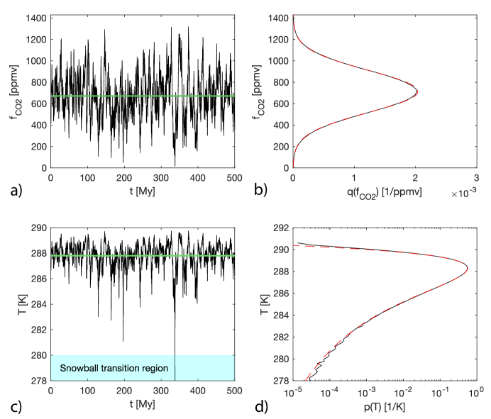
Figure 1.— Output of the numerical stochastic model over 500 My for an ensemble of 1024 runs, given fixed stellar luminosity ($\alpha=0.98$), relaxation timescale $\tau=2.5$ My, and $\sigma_{y}=0.7$. a) CO2 molar concentration vs. time, b) normalized histogram of CO2 molar concentration values, c) temperature vs. time and d) normalized histogram of temperature values. For a) and c), a single run where temperature dropped below the Snowball limit is shown in black. In c) the light blue shading indicates the Snowball transition region, while in both a) and c), the green line indicates the mean value. Finally, in b) and d) the solid black and red dashed lines indicate the numerical results and analytic results according to (6) and (14), respectively. The ice-albedo feedback is not included in these simulations.

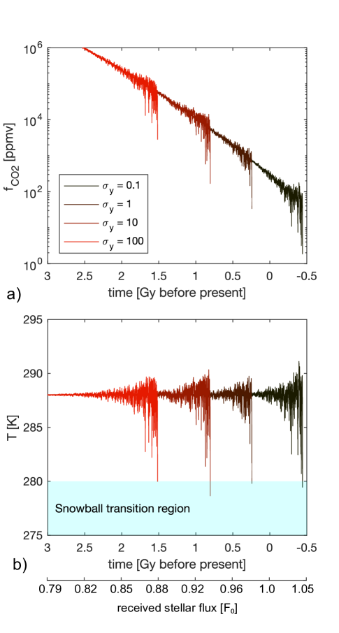
Figure 2.— Output of the numerical stochastic model for an Earth-like planet around a G-star with evolving stellar luminosity over 3.5 Gy, starting from 3 Gy before present. a) Atmospheric CO2 molar concentration and b) global mean temperature as a function of time. Received stellar flux is also shown on the $x$-axis. In b), the light blue shading indicates the Snowball transition region.

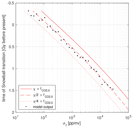
Figure 3.— Time of Snowball transition as a function of CO2 concentration standard deviation $\sigma_{f}$ in ppmv ($\sigma_{f}=\sigma_{y}\times 280$ ppmv). Black dots show numerical model results, while the red lines show fractions of the steady-state parameter $\chi$, which is calculated from (12).

References

- Abbot (2016) D. S. Abbot. Analytical investigation of the decrease in the size of the habitable zone due to a limited \ceCO2 outgassing rate. The Astrophysical Journal, 827(2):117, 2016.
- Arnscheidt and Rothman (2020) C. W. Arnscheidt and D. H. Rothman. Routes to global glaciation. Proceedings of the Royal Society A, 476(2239):20200303, 2020.
- Bean et al. (2017) J. L. Bean, D. S. Abbot, and E. M.-R. Kempton. A statistical comparative planetology approach to the hunt for habitable exoplanets and life beyond the solar system. The Astrophysical Journal Letters, 841(2):L24, 2017.
- Checlair et al. (2017) J. Checlair, K. Menou, and D. S. Abbot. No snowball on habitable tidally locked planets. The Astrophysical Journal, 845(2):132, 2017.
- Cowan et al. (2011) N. B. Cowan, T. Robinson, T. A. Livengood, D. Deming, E. Agol, M. F. A’Hearn, D. Charbonneau, C. M. Lisse, V. S. Meadows, S. Seager, et al. Rotational variability of Earth’s polar regions: implications for detecting snowball planets. 2011.
- Cox et al. (2016) G. M. Cox, G. P. Halverson, R. K. Stevenson, M. Vokaty, A. Poirier, M. Kunzmann, Z.-X. Li, S. W. Denyszyn, J. V. Strauss, and F. A. Macdonald. Continental flood basalt weathering as a trigger for Neoproterozoic Snowball Earth. Earth and Planetary Science Letters, 446:89–99, 2016.
- Feulner (2012) G. Feulner. The faint young Sun problem. Reviews of Geophysics, 50(2), 2012.
- Feulner (2017) G. Feulner. Formation of most of our coal brought Earth close to global glaciation. Proceedings of the National Academy of Sciences, 114(43):11333–11337, 2017.
- Foster and Rahmstorf (2011) G. Foster and S. Rahmstorf. Global temperature evolution 1979–2010. Environmental Research Letters, 6(4):044022, 2011.
- Franks et al. (2014) P. J. Franks, D. L. Royer, D. J. Beerling, P. K. Van de Water, D. J. Cantrill, M. M. Barbour, and J. A. Berry. New constraints on atmospheric \ceCO2 concentration for the Phanerozoic. Geophysical Research Letters, 41(13):4685–4694, 2014.
- Gough (1981) D. O. Gough. Solar interior structure and luminosity variations. In Physics of Solar Variations, pages 21–34. Springer, 1981.
- Graham (2021) R. J. Graham. High p\ceCO2 reduces sensitivity to \ceCO2 perturbations on temperate, Earth-like planets throughout most of habitable zone, 2021. arXiv preprint arXiv:2104.01224.
- Graham and Pierrehumbert (2020) R. J. Graham and R. Pierrehumbert. Thermodynamic and energetic limits on continental silicate weathering strongly impact the climate and habitability of wet, rocky worlds. The Astrophysical Journal, 896(2):115, 2020.
- Guimond and Cowan (2018) C. M. Guimond and N. B. Cowan. The direct imaging search for Earth 2.0: Quantifying biases and planetary false positives. The Astronomical Journal, 155(6):230, 2018.
- Haqq-Misra et al. (2016) J. Haqq-Misra, R. K. Kopparapu, N. E. Batalha, C. E. Harman, and J. F. Kasting. Limit cycles can reduce the width of the habitable zone. The Astrophysical Journal, 827(2):120, 2016.
- Hoffman et al. (1998) P. F. Hoffman, A. J. Kaufman, G. P. Halverson, and D. P. Schrag. A Neoproterozoic Snowball Earth. Science, 281(5381):1342–1346, 1998.
- Huybers and Langmuir (2017) P. Huybers and C. H. Langmuir. Delayed \ceCO2 emissions from mid-ocean ridge volcanism as a possible cause of late-Pleistocene glacial cycles. Earth and Planetary Science Letters, 457:238–249, 2017.
- Jacobs (2010) K. Jacobs. Stochastic processes for physicists: understanding noisy systems. Cambridge University Press, 2010.
- Joshi and Haberle (2012) M. M. Joshi and R. M. Haberle. Suppression of the water ice and snow albedo feedback on planets orbiting red dwarf stars and the subsequent widening of the habitable zone. Astrobiology, 12(1):3–8, 2012.
- Kasting et al. (1993) J. F. Kasting, D. P. Whitmire, and R. T. Reynolds. Habitable Zones around Main Sequence Stars. Icarus, 101:108–128, 1993.
- Kopparapu et al. (2013) R. K. Kopparapu, R. Ramirez, J. F. Kasting, V. Eymet, T. D. Robinson, S. Mahadevan, R. C. Terrien, S. Domagal-Goldman, V. Meadows, and R. Deshpande. Habitable Zones around Main-sequence Stars: New Estimates. The Astrophysical Journal, 765:131, 2013.
- Lehmer et al. (2020) O. R. Lehmer, D. C. Catling, and J. Krissansen-Totton. Carbonate-silicate cycle predictions of Earth-like planetary climates and testing the habitable zone concept. Nature Communications, 11(1):1–10, 2020.
- Lenardic et al. (2016) A. Lenardic, A. M. Jellinek, B. Foley, C. O’Neill, and W. B. Moore. Climate-tectonic coupling: Variations in the mean, variations about the mean, and variations in mode. Journal of Geophysical Research: Planets, 121(10):1831–1864, 2016.
- Lovelock and Margulis (1974) J. E. Lovelock and L. Margulis. Atmospheric homeostasis by and for the biosphere: the Gaia hypothesis. Tellus, 26(1-2):2–10, 1974.
- Lucarini and Bódai (2019) V. Lucarini and T. Bódai. Transitions across melancholia states in a climate model: Reconciling the deterministic and stochastic points of view. Physical Review Letters, 122(15):158701, 2019.
- Lüthi et al. (2008) D. Lüthi, M. Le Floch, B. Bereiter, T. Blunier, J.-M. Barnola, U. Siegenthaler, D. Raynaud, J. Jouzel, H. Fischer, K. Kawamura, and T. F. Stocker. High-resolution carbon dioxide concentration record 650,000–800,000 years before present. Nature, 453(7193):379–382, 2008.
- Macdonald and Wordsworth (2017) F. A. Macdonald and R. Wordsworth. Initiation of Snowball Earth with volcanic sulfur aerosol emissions. Geophysical Research Letters, 44(4):1938–1946, 2017.
- Macdonald et al. (2019) F. A. Macdonald, N. L. Swanson-Hysell, Y. Park, L. Lisiecki, and O. Jagoutz. Arc-continent collisions in the tropics set Earth’s climate state. Science, 364(6436):181–184, 2019.
- Maher and Chamberlain (2014) K. Maher and C. P. Chamberlain. Hydrologic regulation of chemical weathering and the geologic carbon cycle. Science, 343(6178):1502–1504, 2014.
- Montañez et al. (2016) I. P. Montañez, J. C. McElwain, C. J. Poulsen, J. D. White, W. A. DiMichele, J. P. Wilson, G. Griggs, and M. T. Hren. Climate, p\ceCO2 and terrestrial carbon cycle linkages during late Palaeozoic glacial–interglacial cycles. Nature Geoscience, 9(11):824–828, 2016.
- Myhre et al. (1998) G. Myhre, E. J. Highwood, K. P. Shine, and F. Stordal. New estimates of radiative forcing due to well mixed greenhouse gases. Geophysical research letters, 25(14):2715–2718, 1998.
- Pagani et al. (2009) M. Pagani, K. Caldeira, R. Berner, and D. J. Beerling. The role of terrestrial plants in limiting atmospheric \ceCO2 decline over the past 24 million years. Nature, 460(7251):85–88, 2009.
- Pierrehumbert et al. (2011) R. T. Pierrehumbert, D. S. Abbot, A. Voigt, and D. Koll. Climate of the Neoproterozoic. Annual Review of Earth and Planetary Sciences, 39:417–460, 2011.
- Seager (2013) S. Seager. Exoplanet habitability. Science, 340(6132):577–581, 2013.
- Shields et al. (2013) A. L. Shields, V. S. Meadows, C. M. Bitz, R. T. Pierrehumbert, M. M. Joshi, and T. D. Robinson. The effect of host star spectral energy distribution and ice-albedo feedback on the climate of extrasolar planets. Astrobiology, 13(8):715–739, 2013.
- Sigman et al. (2010) D. M. Sigman, M. P. Hain, and G. H. Haug. The polar ocean and glacial cycles in atmospheric \ceCO2 concentration. Nature, 466(7302):47–55, 2010.
- Tajika (2007) E. Tajika. Long-term stability of climate and global glaciations throughout the evolution of the Earth. Earth, Planets and Space, 59(4):293–299, 2007.
- Tierney et al. (2020) J. E. Tierney, J. Zhu, J. King, S. B. Malevich, G. J. Hakim, and C. J. Poulsen. Glacial cooling and climate sensitivity revisited. Nature, 584(7822):569–573, 2020.
- Voigt and Abbot (2012) A. Voigt and D. S. Abbot. Sea-ice dynamics strongly promote Snowball Earth initiation and destabilize tropical sea-ice margins. Climate of the Past, 8(6):2079–2092, 2012.
- Voigt et al. (2011) A. Voigt, D. S. Abbot, R. T. Pierrehumbert, and J. Marotzke. Initiation of a Marinoan Snowball Earth in a state-of-the-art atmosphere-ocean general circulation model. Climate of the Past, 7(1):249–263, 2011.
- Walker et al. (1981) J. C. G. Walker, P. B. Hays, and J. F. Kasting. A negative feedback mechanism for the long-term stabilization of the earth’s surface temperature. Journal of Geophysical Research, 86:9776–9782, 1981.