Self-adaptive loss balanced Physics-informed neural networks for the incompressible Navier-Stokes equations

Abstract

There have been several efforts to Physics-informed neural networks (PINNs) in the solution of the incompressible Navier-Stokes fluid. The loss function in PINNs is a weighted sum of multiple terms, including the mismatch in the observed velocity and pressure data, the boundary and initial constraints, as well as the residuals of the Navier-Stokes equations. In this paper, we observe that the weighted combination of competitive multiple loss functions plays a significant role in training PINNs effectively. We establish Gaussian probabilistic models to define the loss terms, where the noise collection describes the weight parameter for each loss term. We propose a self-adaptive loss function method, which automatically assigns the weights of losses by updating the noise parameters in each epoch based on the maximum likelihood estimation. Subsequently, we employ the self-adaptive loss balanced Physics-informed neural networks (lbPINNs) to solve the incompressible Navier-Stokes equations, including two-dimensional steady Kovasznay flow, two-dimensional unsteady cylinder wake, and three-dimensional unsteady Beltrami flow. Our results suggest that the accuracy of PINNs for effectively simulating complex incompressible flows is improved by adaptively appropriate weights in the loss terms. The outstanding adaptability of lbPINNs is not irrelevant to the initialization choice of noise parameters, which illustrates the robustness. The proposed method can also be employed in other problems where PINNs apply besides fluid problems.

1 Introduction

Incompressible fluids ranging from laminar to turbulent flows are widespread in many disciplines, such as environmental science, energy development, hydrology, and hydrogeology. It is indispensable to simulate the fluid precisely flows in engineering applications, e.g., conduction of heat, a vibration of the circular membrane, and propagation of electromagnetic waves. The Euler equations, advection-dispersion equations, and Navier–Stokes equations govern the fluid dynamics problems, which belong to partial differential equations (PDEs). Numerical simulations on fluid systems quietly rely on solving PDEs with the computational fluid dynamics (CFD) approach, including the finite elements (FE), finite volumes (FV), and finite differences (FD) methods 2003Finite ; 2018Finite ; 2009Finite . These discretization-based methods approximate the solution of PDEs through their values at a set of grid points distributed over the spatial and temporal domain. However, mesh generation for the flows with complicated geometry is often expensive and time-consuming. There are differences between actual mathematical properties of PDEs and approximate difference equations computed with the derivatives of state variables. In particular, the CFD simulations are challenging to solve the ill-posed or moving boundary value problems. To solve inverse problems by CFD method, this firstly requires tedious data assimilation and has no guarantee of convergence 2012A . Hence, the use of CFD models for real-life applications and real-time predictions is limited. It is significant to develop an effective Navier-Stokes solver that could overcome the limitations mentioned above.

One surrogate modeling approach to rapidly attain the solutions of Navier-Stokes equations, such as velocity, the pressure is to build a surrogate model, which learns the initial and boundary constraints from data Wang2016Data ; 2016Reconstruction ; Sean2017Data ; 2019Flowfield ; 2018Deepinverse . Due to the breakthrough approximation capabilities of neural networks MachineLearning ; 2019Subgrid , there have been several remarkable results in solving forward and inverse problems for fluid simulation Data-drivenheattransfer ; 2000Neuralboundary ; HiddenFluidMechanics , instead of using the classical numerical schemes. However, the successful reconstruction of a flow field using neural networks is relevant to sufficient training data. It is challenging to compensate for the incompleteness and sparsity of measurements in many cases, and additional information is required. Recently, there is much effort to investigate physics-based models PIGP ; HiddenPhysicsModels ; PIGAN . The emphasis is on obtaining the best surrogate model constrained by physical laws specified as PDEs besides data. In particular, physics-informed neural networks (PINNs) introduced in raissi2017physics ; raissi2019physics have already become novel PDEs solvers. A series of remarkable results across problems in various fields such as machinery and engineering, including biomedical problems CardiacActivationMapping , finance OptionPricing .

It is suitable for PINNs together with automatic differentiation 2015AutomaticML that does not require mesh generation to solve fluid mechanics problems PIDiagnostics ; largesimulation ; ADE . Jin et al. proposed NSFnets by considering the velocity-pressure (VP) and the vorticity-velocity (VV) formulation of the incompressible Navier-Stokes equations 2020NSFnets . Mao et al. used PINNs to precisely approximate high-speed aerodynamic flows. Specifically, PINNs were employed to learn the value of the unknown parameter in the state equation for the oblique wave problem highspeedflows . Sun et al. proposed physics-constrained DNNs for surrogate modeling of incompressible fluid flows without any data to avoid expensive simulation experiments 0Surrogate . The performance of the physics-constrained data-free DL surrogate model is studied on several flow cases with two idealized vascular geometries. Besides, the overriding concern is that current PINNs lack uncertainty quantification of the solution from the randomness of data or the model architecture restriction. Hence, Sun et al. developed a Physics Constrained Bayesian Neural Network to simulate 2D vascular flows from sparse, noisy velocity measurements. Variational inference UQ2020review was used to estimate the posterior distributions of the reconstructed flow 2020Physics . Zhu et al. raised a Physics-Constrained Deep Learning methodology that simulates high-dimensional porous media flows without labeled data. The quantification and interpretation of the predictive uncertainty are also provided 2019Physics . As for inverse heat transfer applications, Cai et al. employed PINNs to simulate two-dimensional heat transfer in flow past a cylinder without thermal boundaries, which is almost impossible to be solved by classical methods HeatTransfer .

However, the convergence accuracy of baseline PINNs permanently reduced to about $10^{-2}\pm 10^{-3}$, which is a weakness of PINNs raissi2017physics ; raissi2019physics . Therefore, it is necessary to raise the precision of PINNs from the essence of the method. Incorporating the governing equations, initial, and boundary constraints into the loss functions is the main feature of the physical model. The training process that minimizes the multiple loss functions could be regarded as a multi-objective task, challenging for global optimization methods, such as Adam, Stochastic Gradient Descent (SGD), and L-BFGS SGD ; 2014Adam ; 2015Stochastic . Numerical experiments demonstrate that the performance of PINNs is closely linked with the appropriate combination of each loss term. There is no question that workforce to tune weights always time-consuming, laborious, and prone to errors and omissions. Besides, if gradient descent methods optimize the multiple objectives composed with fixed weights, it is quite possible to attain a locally optimal solution elhamod2020cophypgnn . So far, there have been several efforts to integrating sustainable, balanced learning of loss function in PINNs, such as the Neural Tangent Kernel(NTK) principle NTK , the training gradients wang2020understanding , and the network weights Self-Adaptive . Alex et al. observed that the optimal weighting of Multi-Task Learning is relevant to the magnitude of the task’s noise kendall2018multitask . Furthermore, the noise collection describes the weight parameter for each loss term by establishing Gaussian probabilistic models. From a different perspective, we provide a principled way of combining multiple loss functions with learning these competing loss terms in PINNs simultaneously.

In this work, we propose a self-adaptive loss balanced method for PINNs (lbPINNs), which automatically updates weights for each loss term in each iteration. We establish Gaussian probabilistic models to define complex loss functions based on maximum likelihood inference. Using a dynamic noise parameter collection determines the uncertainty of loss during training. The optimal weight of each loss constant depends on the magnitude of the noise parameter. We observe that the loss would be paid a severer penalty when the noise was declining. The primary goal is to improve the approximation capabilities of PINNs. The basic principle in lbPINNs is to tune the observation noise configuration of the model with gradient descent methods together with the training process. The effectiveness and merits of the proposed method are demonstrated by investigating several laminar flows, including two-dimensional steady Kovasznay flow, two-dimensional unsteady cylinder wake, and three-dimensional unsteady Beltrami flow. Compared with the baseline PINNs, the results show that the absolute error of self-adaptive loss-balanced PINNs can permanently be reduced to $10^{-4}\pm 10^{-5}$ in the identical experimental condition. To prove the adaptability of the method, we investigate the influence of initial noise parameters in the loss function on the accuracy of lbPINNs. All performance is better than the baseline PINNs.

The paper is organized as follows. We first provide a detailed introduction to recent related work focused on balancing loss terms in PINNs in section 2. Section 3 introduces the framework of physics-informed neural networks for the incompressible Navier-Stokes equations and the principle of the self-adaptive loss balanced method for PINNs. In Section 4, numerical results of the developed approach on several incompressible Navier-Stokes flows are presented. Section 5 concludes the paper.

2 Related Work

The original PINNs algorithm has successful applications in Navier–Stokes, stochastic PDEs PIGAN ; FokkerPlanck ; FBSNN ; 2019Learning ; 2019Quantifying , and fractional PDEs fPINNs . However, it has been argued that the convergence and accuracy of PINNs still of tremendous challenge. There is no doubt that PINNs are obtained to minimize loss functions defined by the sampled data and physical laws that add to prior knowledge of PDEs. Zhao et al. observed that the combination of multiple loss functions plays a significant role in the convergence of PINNs wight2020solving . In particular, more work has been devoted to balancing the interplay among loss terms in PINNs automatically through the training process.

Recently, wang et al. provided a learning rate annealing algorithm that uses the back-propagated gradient statistics in the training procedure wang2020understanding . It is widely acknowledged that the behavior of PINNs during model training via gradient descent is still a vague issue. The problems of vanishing gradient and exploding gradient would limit the application of this method. Hence the Neural Tangent Kernel(NTK) Perspective was presented to understanding the training process for PINNs NTK . A practical technique based on the NTK perspective that appropriately assigns weights to each loss item was proposed. Since the distribution of eigenvalues of the NTK never changes, the performance improvement is quietly slight. Shin et al. proved the convergence theory for data-driven PINNs and derived the Lipschitz Regularized loss to solving linear second-order elliptic and parabolic type PDEs 2020On . A method that updates the adaptation weights in the loss function concerning the network parameters was suggested Self-Adaptive . In general, the Self-Adaptive PINNs were forced to meet physical constraints as far as possible by minimizing the loss, where the trainable weights increase corresponding to higher loss. Hence the procedure could be remarked as a penalty PDE-constrained optimization problem.

Although there have been many studies to verify the effects of loss on generalization performance, the competitive relationship between physics objectives loss items is not considered. Bu et al. pointed out that it is crucial to tune the competing physics-guided (PG) loss functions at various neural network learning stages elhamod2020cophypgnn . Therefore, two approaches named annealing and cold starting that affect the initial or last epochs were proposed to tune the trade-off weights of loss terms with some different characteristics. However, it would be tedious to choose the appropriate kind of sigmoid function, which primarily influences accuracy. By careful consideration of competitiveness and adaptability, we get inspiration from multi-task learning and provide a self-adaptive loss balanced method for PINNs, which use uncertainty to weigh multiple losses automatically. We mainly investigate the possibility of using lbPINNs to approximate the incompressible Navier-Stokes equations that model laminar and turbulent flows.

3 Methods

3.1 Physics-informed neural networks for the Navier-Stokes equations

The physics-informed neural networks have been widely used as a data-driven method for solving general nonlinear partial differential equations, such as the Burgers equation, Poisson equation, and Schrodinger equation raissi2017physics ; raissi2019physics . We introduce physics-informed neural networks for the incompressible three-dimensional Navier-Stokes, reflecting the basic mechanics of viscous fluid flow. We model the fluid dynamics by the three-dimensional NS equations with the Newtonian assumption:

$$\frac{\partial\mathbf{u}}{\partial t}+(\mathbf{u}\cdot\nabla)\mathbf{u} =-\nabla p+\frac{1}{\operatorname{Re}}\nabla^{2}\mathbf{u}\quad\text{ in }\Omega,$$ (1)

$$\nabla\cdot\mathbf{u} =0\quad\text{ in }\Omega,$$

$$\mathbf{u} =\mathbf{u}_{\Gamma}\quad\text{ on }\Gamma_{D},$$

$$\frac{\partial\mathbf{u}}{\partial n} =0\quad\text{ on }\Gamma_{N},$$

$$\mathbf{u}(\bm{x},0) =\mathbf{h}(\bm{x}),\quad\text{ in }\Omega,$$

where $\bm{x}=[x,y,z]\in\Omega$ and $t\in[0,T]$ denote space and time coordinates. Respectively, the Reynolds number $Re=U_{ref}D_{ref}/\upsilon$ is defined by kinematic viscosity $\upsilon$, characteristic length $D_{ref}$, and reference velocity $U_{ref}$ of the fluid. The continuity equation of an incompressible fluid is considered, which describes the conservation of fluid mass. $\Gamma_{D}$ and $\Gamma_{N}$ are the Dirichlet and Neumann boundaries of the computational domain. The scalar $\bm{h}(\bm{x})$ is the initial constraints. $u(x,y,z,t)$, $v(x,y,z,t)$, and $w(x,y,z,t)$ represent the $x,y$, and $z$ component of the velocity field. $p(x,y,z,t)$ represents the pressure.

Following the original work of raissi2017physics , the solution of Navier-Stokes equations (1) could be approximated by neural network $\hat{\bm{u}}(\bm{x},t;\theta)$. There are some advanced deep learning architectures, like Fourier Network2020Fourier , DGM 2018DGM , and sinusoidal representation network (Siren) 2020Implicit . In its simplest form, we consider the feed-forward fully connected neural network of depth $M$, which takes the input $x,y,z,t$ and denote the output of the $m-th$ layer as $\hat{\bm{u}}^{[m]}$. The neural network is defined as:

$$\text{ input layer:}\quad\hat{\bm{u}}^{[m]}= x,$$ (2)

$$\text{ hidden layers:}\quad\hat{\bm{u}}^{[m]}= \sigma\left(W^{[m]}\hat{u}^{[m-1]}+b^{[m]}\right),$$

$$\quad\text{ for }m=2,3,\cdots,M-1,$$

$$\text{ output layer:}\quad\hat{\bm{u}}^{[M]}= \left(W^{[M]}\hat{u}^{[M-1]}+b^{[M]}\right),$$

where $\sigma$ is the activation function including sigmoid, relu, and tanh 2018Activation ; 2017Searching . $W^{[m]}$ and $b^{[m]}$ represent the weights and biases at $m-th$ layer. All weight matrices and bias vectors could be denoted by a parameter collection $\theta=\left\{W^{[m]},b^{[m]}\right\}_{1\leq m\leq M}$. Define the residuals as:

$$\bm{f}_{1}(\bm{x},t;\theta): =\frac{\partial\mathbf{u}}{\partial t}+(\mathbf{u}\cdot\nabla)\mathbf{u}+\nabla p-\frac{1}{\operatorname{Re}}\nabla^{2}\mathbf{u},$$ (3)

$$\bm{f}_{2}(\bm{x},t;\theta): =\nabla\cdot\mathbf{u}.$$

Automatic differentiation (AD) could take all partial derivatives, which has been integrated into PyTorch 2015AutomaticML . Prior knowledge of physics was integrated into the loss function. The framework of physics-informed neural networks for the incompressible Navier-Stokes equations is constructed shown in figure 1. The best parameter collection $\theta^{\ast}$ is identified by minimizing multiple loss functions as follows:

$$L(\theta;N) =\omega_{f}L_{PDE}\left(\theta;N_{f}\right)+\omega_{b}L_{BC}\left(\theta;N_{b}\right)$$ (4)

$$+\omega_{i}L_{IC}\left(\theta;N_{i}\right)+\omega_{d}L_{data}\left(\theta;N_{data}\right),$$

where $\omega=\left\{\omega_{f},\omega_{b},\omega_{i},\omega_{d}\right\}$ contains weights of each loss term. The number of training points is concluded by parameter $N=\left\{N_{f},N_{b},N_{i},N_{data}\right\}$. The loss $L_{PDE}$ penalizes the Navier-Stokes residuals; The loss $L_{BC}$ aims to fit the Dirichlet boundary $\Gamma_{D}$ or Neumann boundary $\Gamma_{N}$. The loss $L_{IC}$ determines the error of the initial constraints. The loss $L_{data}$ is computed corresponding to sample data:

$$L_{PDE}\left(\theta;N_{f}\right) =\frac{1}{\left|N_{f}\right|}\sum_{j=1}^{N_{f}}\|\bm{f}_{1}(\bm{x}_{f}^{j},t_{f}^{j};\theta)\|^{2}+\|\bm{f}_{2}(\bm{x}_{f}^{j},t_{f}^{j};\theta)\|^{2},$$ (5)

$$L_{BC}\left(\theta;N_{b}\right) =\frac{1}{\left|N_{b}\right|}\sum_{j=1}^{N_{b}}\|\hat{\bm{u}}(\bm{x}_{b}^{j},t_{b}^{j};\theta)-\bm{g}_{b}^{j}\|^{2},$$

$$L_{IC}\left(\theta;N_{i}\right) =\frac{1}{\left|N_{i}\right|}\sum_{j=1}^{N_{i}}\|\hat{\bm{u}}(\bm{x}_{i}^{j},0;\theta)-\bm{h}_{i}^{j}\|^{2},$$

$$L_{data}\left(\theta;N_{data}\right) =\frac{1}{\left|N_{data}\right|}\sum_{j=1}^{N_{data}}\|\hat{\bm{u}}(\bm{x}_{data}^{j},t_{data}^{j};\theta)-\bm{u}_{data}^{j}\|^{2},$$

where $\left\{\bm{x}_{f}^{j},t_{f}^{j}\right\}^{N_{f}}_{j=1}$ is a set of collocation points that are uniformly sampled inside the domain $\Omega$. The collection $\left\{\bm{x}_{b}^{j},t_{b}^{j},\bm{g}_{b}^{j}=\bm{g}(\bm{x}_{b}^{j},t_{b}^{j})\right\}^{N_{b}}_{j=1}$ donates the boundary constraint points. The collection $\left\{\bm{x}_{i}^{j},\bm{h}_{i}^{j}\right\}^{N_{i}}_{j=1}$ donates the initial constraint points. The dataset $\left\{\bm{x}_{data}^{j},t_{data}^{j},\bm{u}_{data}^{j}\right\}^{N_{data}}_{j=1}$ is sample points. The parameters $N_{f},N_{b},N_{i},N_{data}$ are the total number of points. The Physics-informed neural networks (PINNs) for the incompressible Navier-Stokes equations algorithm is summarized as follows.

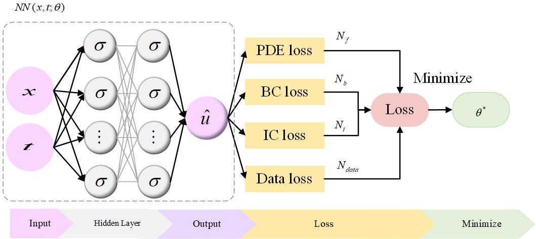
Figure 1: A schematic diagram of the physics-informed neural networks (PINNs) for the incompressible Navier-Stokes equations.

Algorithm 1 Physics-informed neural networks (PINNs)

Training steps S, the learning rate $lr$, weight collection $\omega$ used to balance the interplay between the different loss terms.

Find the best model with parameters $\theta^{\ast}$

Step  1:Specify the training set

Initial constraint points: $\left\{\bm{x}_{i}^{j},\bm{h}_{i}^{j}\right\}^{N_{i}}_{j=1}$.

Boundary constraint points: $\left\{\bm{x}_{b}^{j},t_{b}^{j},\bm{g}_{b}^{j}\right\}^{N_{b}}_{j=1}$.

Training points: $\left\{\bm{x}_{data}^{j},t_{data}^{j},\bm{u}_{data}^{j}\right\}^{N_{data}}_{j=1}$.

Residual training points: $\left\{\bm{x}_{f}^{j},t_{f}^{j}\right\}^{N_{f}}_{j=1}$.

Step  2: Construct the neural network $\hat{\bm{u}}(\bm{x},t;\theta)$ with random initialization of parameters $\theta$ (2).

Step  3:Define the residuals (3) using automatic differentiation and other arithmetic operations.

Step  4:Use S steps of a gradient descent algorithm to update the parameters $\theta$ as:

for $s=1$ to $S$ do

     (a) Specify the loss function $L(\theta_{s};N)$ (4) with the weight collection $\omega$ based on equation (5).

     (b) Update the parameters $\theta$ using Adam with the learning rate $lr$ for minimizing the loss function.

                $\theta_{s+1}\leftarrow$ Adam $(L(\theta_{s};N);lr)$

end for

Table 1: Comparing the results with different weights constant when learning 2d Kovasznay flow with PINNs. The weight selection $[\omega_{f},\omega_{b}]=[0.25,0.75]$ achieves the best accuracy, which is bold in this table.

Fixed weights $\omega_{f},\omega_{b}$	$error_{u}$	$error_{v}$	$error_{p}$
$[1.0,1.0]$	$4.06030e-03$	$2.87294e-03$	$4.43514e-03$
$[0.85,0.15]$	$6.60475e-03$	$4.69625e-02$	$7.41679e-02$
$[0.15,0.85]$	$3.83967e-03$	$5.79027e-03$	$3.84211e-02$
$[0.75,0.25]$	$1.88834e-03$	$1.97016e-03$	$4.05601e-02$
$[0.25,0.75]$	$1.08440e-03$	$2.10914e-03$	$1.88593e-03$
$[0.65,0.35]$	$8.46328e-03$	$2.59047e-03$	$1.97016e-02$
$[0.35,0.65]$	$1.94430e-03$	$3.70284e-03$	$4.88638e-03$

3.2 Self-adaptive loss balanced method

The most common way to combine losses of each constraint is the weighted summation. To verify the impact of weight allocations, we simulated the 2d steady Kovasznay flow with different weight coefficients on the baseline PINNs. Here the weights are only considered $\omega_{f},\omega_{b}$ and add up to one. As the experimental results shown in table 1, we found that the performance and convergence of PINNs were susceptible to various loss weight selections. It is obvious that $[\omega_{f},\omega_{b}]=[0.25,0.75]$ achieve the best accuracy in this table. Besides, it could be expensive to manually tune these weight hyper-parameters, especially for complex fluid dynamics. Therefore, it is desirable to propose a more convenient and principled to learn these weights adaptively, achieving the balance between each competing physics objective.

Our idea is inspired by a paper that presents a principled strategy to weigh multiple loss functions in the scene geometry, and semantics multi-task deep learning problem kendall2018multitask . The loss function is defined based on maximizing the Gaussian likelihood with the homoscedastic uncertainty. As is illustrated in figure 2, let us claim that the sources of uncertainty in Bayesian modeling are divided into two parts kendall2017uncertainties . The first one, conceptually named epistemic uncertainty (also known as knowledge uncertainty), indicates the uncertainty of the model. Inadequate training data and knowledge always cause it. Thus it could be explained away when data are enough. Another type of uncertainty is aleatoric uncertainty (also known as data uncertainty), which captures the inherent property of data distribution and cannot be reduced even though more data were provided. Further, there are two subcategories of aleatoric uncertainty. The heteroscedastic uncertainty depends on the input data. It shows better performance when parts of the observation space have high noise levels. At the same time, homoscedastic uncertainty would stay constant for various inputs and varies between different tasks.

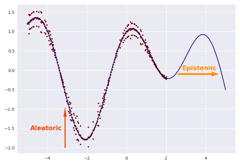
Figure 2: View of the main differences between aleatoric and epistemic uncertainties. Aleatoric uncertainty captures the inherent property of data distribution and cannot be reduced even though more data were provided. Epistemic uncertainty indicates the uncertainty of the model and could be explained away when data are enough.

As for regression tasks on solving Navier-Stokes equations, the likelihood is defined as a Gaussian with mean given by the surrogate model output $\hat{\bm{u}}(\bm{x},t;\theta)$. The parameter $\varepsilon$ is the observation noise in the output to determines the uncertainty:

$$\begin{array}[]{c}p\left(y\mid\hat{\bm{u}}(\bm{x},t;\theta)\right)=N\left(\hat{\bm{u}}(\bm{x},t;\theta),\varepsilon^{2}\right).\end{array}$$ (6)

Consider the output follows Gaussian distribution. The noise scalar $\varepsilon$ is often fixed as part of the weight decay of neural networks. To capture aleatoric uncertainty with dependent data, we would tune the observation noise parameter based on maximum likelihood inference. Due to the minimization objective, the negative log-likelihood of the model is written askendall2017uncertainties :

$$-\log p\left(y\mid\hat{\bm{u}}(\bm{x},t;\theta)\right) \propto\frac{1}{2\varepsilon^{2}}\left\|y-\hat{\bm{u}}(\bm{x},t;\theta)\right\|^{2}+\log\varepsilon$$ (7)

$$=\frac{1}{2\varepsilon^{2}}L_{1}(\theta)+\log\varepsilon,$$

where the loss $L_{1}(\theta)$ represents the output variable. Equation (7) is composed of the residual regression and uncertainty regularization term to adapt the residual weights automatically. This idea is extended to the loss function of PINNs and read as follows:

$$L(\varepsilon;\theta;N) =\frac{1}{2\varepsilon_{f}^{2}}L_{PDE}\left(\theta;N_{f}\right)+\frac{1}{2\varepsilon_{b}^{2}}L_{BC}\left(\theta;N_{b}\right)$$ (8)

$$+\frac{1}{2\varepsilon_{i}^{2}}L_{IC}\left(\theta;N_{i}\right)+\frac{1}{2\varepsilon_{d}^{2}}L_{data}\left(\theta;N_{data}\right)$$

$$+\log\varepsilon_{f}\varepsilon_{b}\varepsilon_{i}\varepsilon_{d},$$

where the collection $\varepsilon=\left\{\varepsilon_{f},\varepsilon_{b},\varepsilon_{i},\varepsilon_{d}\right\}$ describes noise parameters for each loss term. Similarly, the objective is to find the best model weights $\theta^{\ast}$ and noise scalar $\varepsilon^{\ast}$ by minimizing the loss $L(\varepsilon;\theta;N)$ with gradient-based optimizers, such as Stochastic Gradient Descent (SGD), Adam, and L-BFGS SGD ; 2014Adam ; 2015Stochastic . On the one hand, for instance, $\varepsilon_{f}$ decreases, the weight of $L_{PDE}$ increases, which means more punitive to the $L_{PDE}$. The last term $\log\varepsilon_{f}$ regulates the $\varepsilon_{f}$. Thus the noise is discouraged from increasing too much. On the other hand, large uncertainty decreases the contribution of terms, whereas small scale would increase its contribution and penalizes the model. Moreover, the illustration of lbPINNs is shown in figure 3. We learn the relative weight of loss items adaptively when we optimize the noise scalar $\varepsilon$ and the model vector $\theta$, which allows us to learn the weights of each loss in a principled and persuasive way. The Self-adaptive loss balanced method for the PINNs algorithm is summarized.

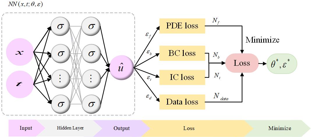
Figure 3: Illustration of Self-adaptive loss balanced Physics-informed neural networks (lbPINNs).

Algorithm 2 Self-adaptive loss balanced method for PINNs

Training steps S, the learning rate $lr$, initial values for the noise collection $\varepsilon=\left\{\varepsilon_{f},\varepsilon_{b},\varepsilon_{i},\varepsilon_{d}\right\}$.

Find the best model with parameters $\theta^{\ast}$ and the excellent noise scalar $\varepsilon^{\ast}$.

Step  1:Consider a physics-informed neural network $\hat{\bm{u}}(\bm{x},t;\theta)$ with initial parameters $\theta$.

Step  2:Construct a Gaussian probabilistic model (6) with mean given by the output of PINNs and the noise collection $\varepsilon$.

Step  3:Then use S steps of a gradient descent algorithm to update the parameters $\varepsilon$ and $\theta$ as:

for $s=1$ to $S$ do

     (a) Define the weighted loss function $L(\varepsilon_{s};\theta_{s};N)$ (8) based on the maximum likelihood estimation (7).

     (b) Tune the noise parameters $\varepsilon$ via Adam to maximize the probability of meeting constraints.

                $\varepsilon_{s+1}\leftarrow$ Adam $(L(\varepsilon_{s};\theta_{s};N);lr)$

     (c) Update the parameters $\theta$ via Adam.

                $\theta_{s+1}\leftarrow$ Adam $(L(\varepsilon_{s};\theta_{s};N);lr)$

end for

4 Results

In this section, we test the original PINNs with different weight selections $\omega$ for the sake of contrasting their capability to represent manifold equations with lbPINNs. We aim to highlight the ability of our method to handle the classical Navier–Stokes equations, which are closely related to the physics of many scientific phenomena. The completed Navier–Stokes equation is often valid for engineering interests, such as vascular flow studies, Molecular diffusion analysis, airplane, and automobile design. We apply the proposed lbPINNs to simulate different incompressible Navier-Stokes flows. First, we consider two-dimensional steady Kovasznay flow with the analytic solution to investigate the effectiveness of lbPINNs based on boundary constraints. Then we employ the self-adaptive loss balanced method to unsteady cylinder wake in two dimensions. Finally, the three-dimensional unsteady Beltrami flow is also successfully simulated by lbPINNs, which considers initial and boundary constraints. CFD simulations provide all collocation points raissi2019physics .

To illustrate the efficiency of the proposed method, the accuracy of the trained model is assessed through the relative L2 error of the exact value $\bm{u}(\bm{x}_{i},t_{i})$ and the trained approximation $\hat{\bm{u}}\left(\bm{x}_{i},t_{i}\right)$ inferred by the network at the data points $\left\{\bm{x}_{i},t_{i}\right\}^{N}_{i=1}$. Various comparisons and detailed numerical experimental results on the Navier–Stokes equation are provided as follows.

$$\text{ L2 error }=\frac{\sqrt{\sum_{i=1}^{N}\left|\hat{\bm{u}}\left(\bm{x}_{i},t_{i}\right)-\bm{u}\left(\bm{x}_{i},t_{i}\right)\right|^{2}}}{\sqrt{\sum_{i=1}^{N}\left|\bm{u}\left(\bm{x}_{i},t_{i}\right)\right|^{2}}}.$$ (9)

Table 2: Comparing the results with multiple initial noise configurations when learning 2d Kovasznay flow.

Initial settings	Excellent settings	$Loss_{PDE}$	$Loss_{BC}$
$[0.02,0.02]$	$[2.476e-02,9.472e-02]$	$4.0734e-04,$	$6.006e-03$
$[0.2,0.2]$	$[1.866e-02,1.996e-02]$	$1.070e-04$	$5.322e-03$
$[2,2]$	$[1.945e-02,8.095e-02]$	$1.619e-04$	$2.332e-03$

4.1 Kovasznay flow

In this example, we aim to emphasize the proposed methods to simulate the 2d steady Kovasznay flow that belongs to the incompressible Navier-Stokes flows. The analytic solution of velocity and pressure are given as follows 2010An :

$$u(x,y)= 1-e^{\lambda x}\cos(2\pi y),$$ (10)

$$v(x,y)= \frac{\lambda}{2\pi}e^{\lambda x}\sin(2\pi y),$$

$$p(x,y)= \frac{1}{2}\left(1-e^{2\lambda x}\right),$$

$$where\quad\lambda= \frac{1}{2\nu}-\sqrt{\frac{1}{4\nu^{2}}+4\pi^{2}},\quad\nu=\frac{1}{\operatorname{Re}}=\frac{1}{40}.$$

The computational domain is $[-0.5,1]\times[-0.5,1.5]$. Let us consider the prediction scenario in which the 4-layer network is fully connected with 50 neurons per layer and a hyperbolic tangent activation function. There is no initial constraint for this steady flow. Specifically, the number of points selected for the trials shown is $N_{b}=101,N_{f}=2601$. The self-adaptive loss function is combined by PDE and boundary loss with $\varepsilon=[\varepsilon_{f},\varepsilon_{b}]$. We train this network for 1k epochs by minimizing the multiple loss equations using Adam optimizer with a learning rate of $0.001$. First, to explore the influence of $[\varepsilon_{f},\varepsilon_{b}]$ with different initial settings, we take several sets of initial noise configurations in which $\varepsilon_{f}=\varepsilon_{b}$. The results, including the excellent settings, PDE, and boundary loss, are demonstrated in table 2. We find that the final configuration of $\varepsilon$ always achieves $10^{-2}$. The error of PDE residual and boundary is in the range $10^{-3}\pm 10^{-4}$.

Setting initial collection as $[\varepsilon_{f},\varepsilon_{b}]=[2,2]$. The number of the test dataset is $101$. Finally, We achieved an L2 error of $6.411\times 10^{-4}\pm 4.320\times 10^{-5}$ after 1k iterations, which is lower than the final errors of the baseline PINNs $4.435\times 10^{-3}\pm 2.872\times 10^{-3}$ over the same epochs. Figure 4 summarizes the predicted solution and the comparison with actual solutions of velocity $u(x,y)$, $v(x,y)$. We present the approximation of pressure $p(x,y)$ using lbPINNs and the exact solution in figure 5. The relative error of the velocity and pressure for PINNs and lbPINNs are illustrated in table 3. We observe that the error of $u,v$, and $p$ achieve $10^{-4}\pm 10^{-5}$, demonstrating the effectiveness of dynamic weights. Additionally, the convergence of lbPINNs is more quickly than PINNs. The convergence of loss, noise constants, and weights during the training process are displayed in figure 6. The most efficient noise configurations are in range $[5.102\times 10^{-2}\pm 1.945\times 10^{-2},4.075\times 10^{-2}\pm 2.127\times 10^{-2}]$. Finally, all weights achieve $10^{3}$. The convergence of PDE and boundary loss depends on the dynamic noise configurations. The scalar $\varepsilon_{f}$ decreases rapidly and more punitive to the loss $L_{PDE}$, which leads to faster convergence. The test loss of PINNs would attain $1.923\times 10^{-3}$, while lbPINNs would converge to $1.106\times 10^{-3}$.

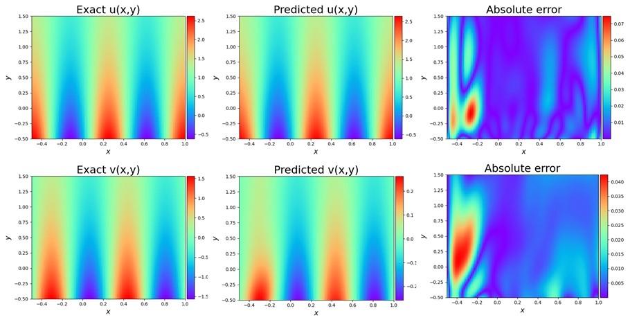
Figure 4: The exact velocity $u(x,y)$, $v(x,y)$ (left), lbPINNs solution (middle), absolute error(right) for the two-dimensional Kovasznay flow across the space domain.

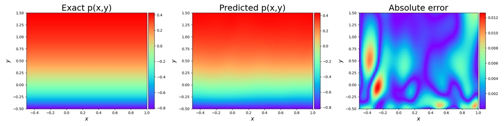
Figure 5: Contrast exact solution(left) of pressure $p(x,y)$ for the two-dimensional Kovasznay flow with the result obtained by lbPINNs (middle) based on the numerical error (right).

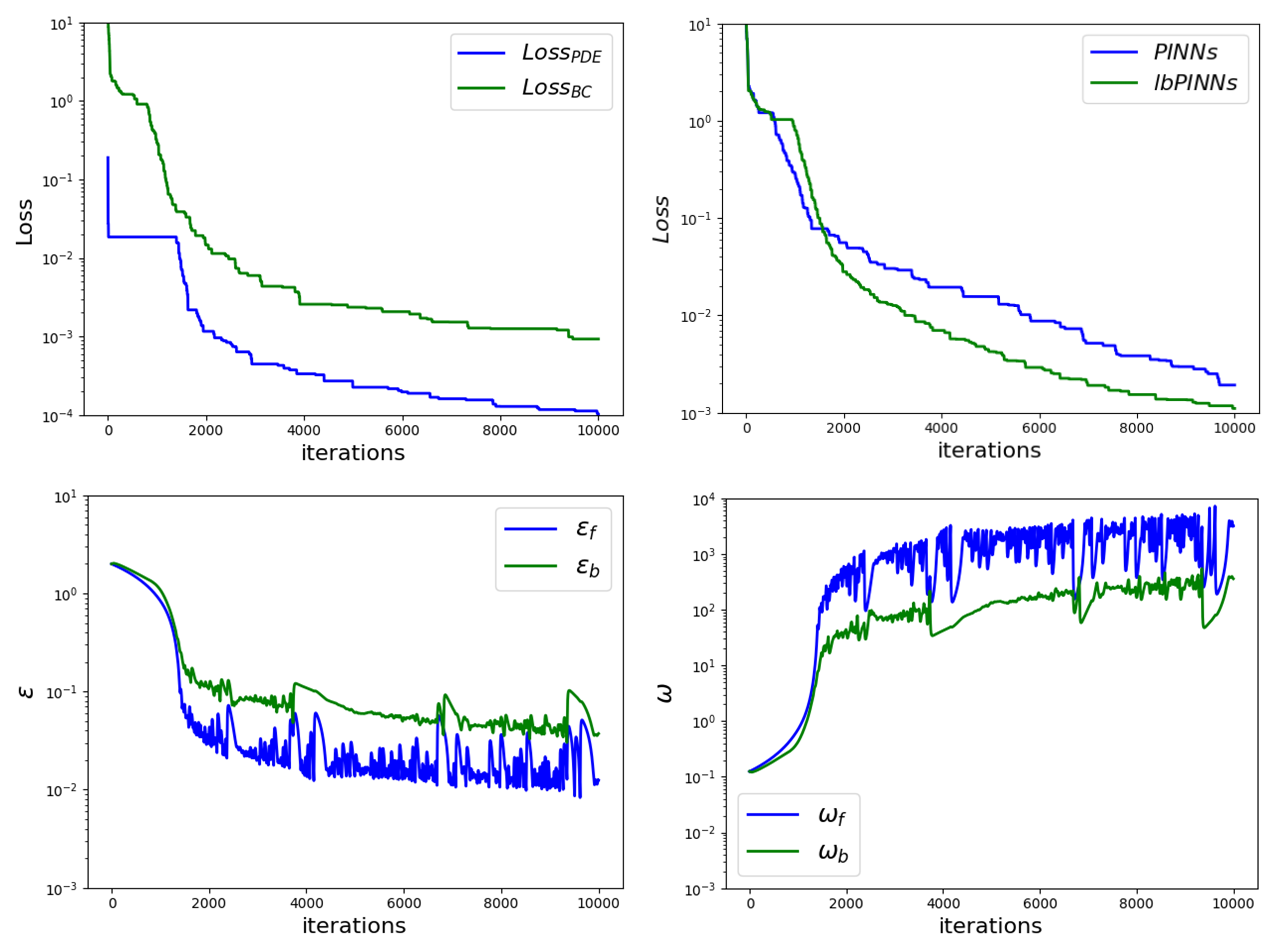
Figure 6: $Loss_{PDE},Loss_{BC}$, $\varepsilon_{f},\varepsilon_{b}$ and $\omega_{f},\omega_{b}$ diagrams for the two-dimensional Kovasznay flow are shown. Besides, the convergence of PINNs and lbPINNs are displayed.

Table 3: Comparing the error for the velocity and pressure when learning 2d Kovasznay flow by PINNs with different weight selections $[\omega_{f},\omega_{b}]$ and lbPINNs with different initial noise configuration $[\varepsilon_{f},\varepsilon_{b}]$.

Methods	parameter selections	$error_{u}$	$error_{v}$	$error_{p}$
PINNs	$[1,1]$	$4.06030e-03$	$2.87294e-03$	$4.43514e-03$
PINNs	$[10,10]$	$5.18614e-03$	$1.58971e-03$	$2.50950e-03$
lbPINNs	$[2,2]$	$6.41112e-04$	$2.81905e-04$	$4.32069e-05$
lbPINNs	$[0.2,0.2]$	$2.15542e-04$	$3.26974e-04$	$3.27784e-05$

Table 4: Apply multiple initial noise settings to simulate cylinder wake by lbPINNs.

Initial settings	Excellent settings	$Loss_{PDE}$	$Loss_{data}$
$[0.2,0.04]$	$[1.447e-02,8.240e-02]$	$2.921e-04$	$1.907e-04$
$[2,2]$	$[9.964e-02,4.421e-02]$	$1.051e-03$	$7.882e-05$
$[2,0.04]$	$[9.189e-02,5.360e-02]$	$6.987e-03$	$6.828e-04$

4.2 cylinder wake

A two-dimensional incompressible flow and dynamic vortex shedding past a circular cylinder in a steady-state are numerically simulated using the spectral/hp element method to validate our predictions. Respectively, the Reynolds number of the incompressible flow is $Re=100$. The kinematic viscosity of the fluid is $\upsilon=0.01$. The cylinder diameter $D$ is $1$. The simulation domain size is $[-15,25]\times[-8,8]$, consisting of 412 triangular elements. Uniform velocity is imposed at the left boundary. Use the periodic boundary constraint on the top and bottom boundaries. A zero-pressure boundary is prescribed at the right boundary.

The deep neural network architecture is fully connected with layer sizes $[3,20,20,20,20,20,20,20,20,2]$ and hyperbolic tangent nonlinearity. A physics-informed neural network model is trained 10k Adam iterations to approximate the latent solution $u(x,y,t),v(x,y,t)$, and $p(x,y,t)$ by formulating the composite loss. We sample $N_{f}=4000$ collocation points, $N_{data}=1000$ exact points. Numerical results of the Navier–Stokes equation in the way of the self-adaptive lbPINNs initialized with splendid initial noise settings are displayed in table 4. The final configuration of parameter $\varepsilon$ also always achieves $10^{-2}$. The error of PDE residual and data are in range $10^{-3}\pm 10^{-5}$.

We demonstrate the results of initial noise parameters $[\varepsilon_{f},\varepsilon_{d}]=[2,2]$ in detail. We present a comparison between the exact and the predicted solutions of stream-wise $u(x,y,t)$ and transverse velocity $v(x,y,t)$ at time instants $t=4s$. A more detailed assessment of the absolute error is displayed in the right panel of figure 7. In table 5, the resulting prediction error of velocity is measured at $4.818\times 10^{-6}\pm 4.564\times 10^{-6}$ in the relative L2-norm, while the original PINNs only converges to $5.321\times 10^{-4}\pm 3.753\times 10^{-4}$. That means extremely higher accuracy than the baseline PINNs. Based on the predicted versus instantaneous pressure field $p(x,y,t)$ shown in figure 8, the error between the predicted value and the true value is extremely low in the entire calculation domain. The convergence of $error_{u},error_{v}$, and $error_{p}$ are shown in figure 9. Through observing the loss and noise parameters curves, we found that relative rates of loss items have evened out around 10k iterations, which indicates the customary efficiency of lbPINNs. It is necessary to demonstrate the adaptive procedure of two noise scalars, and the final result is $[9.964\times 10^{-2}\pm 8.240\times 10^{-2},7.388\times 10^{-2}\pm 4.315\times 10^{-2}]$. As expected, PINNs can accurately capture the complex nonlinear behavior of the Navier–Stokes equation with the self-adaptive loss function.

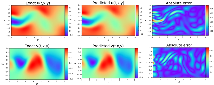
Figure 7: Navier–Stokes equation:Contrast exact stream-wise velocity $u(x,y,t)$, (left) with the result obtained by lbPINNs (middle) based on the absolute error (right).

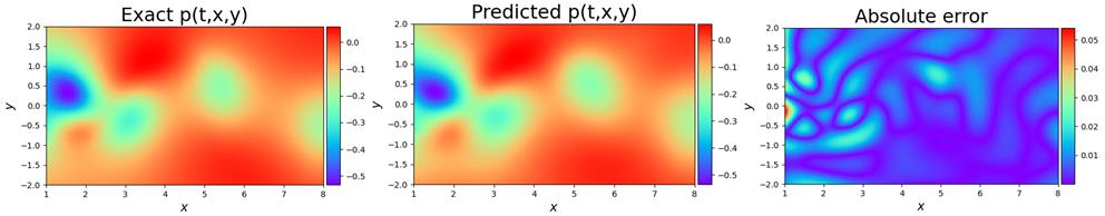
Figure 8: Navier–Stokes equation:Contrast exact pressure $p(x,y,t)$ (left) with the result approximated by lbPINNs (middle) based on the absolute error (right).

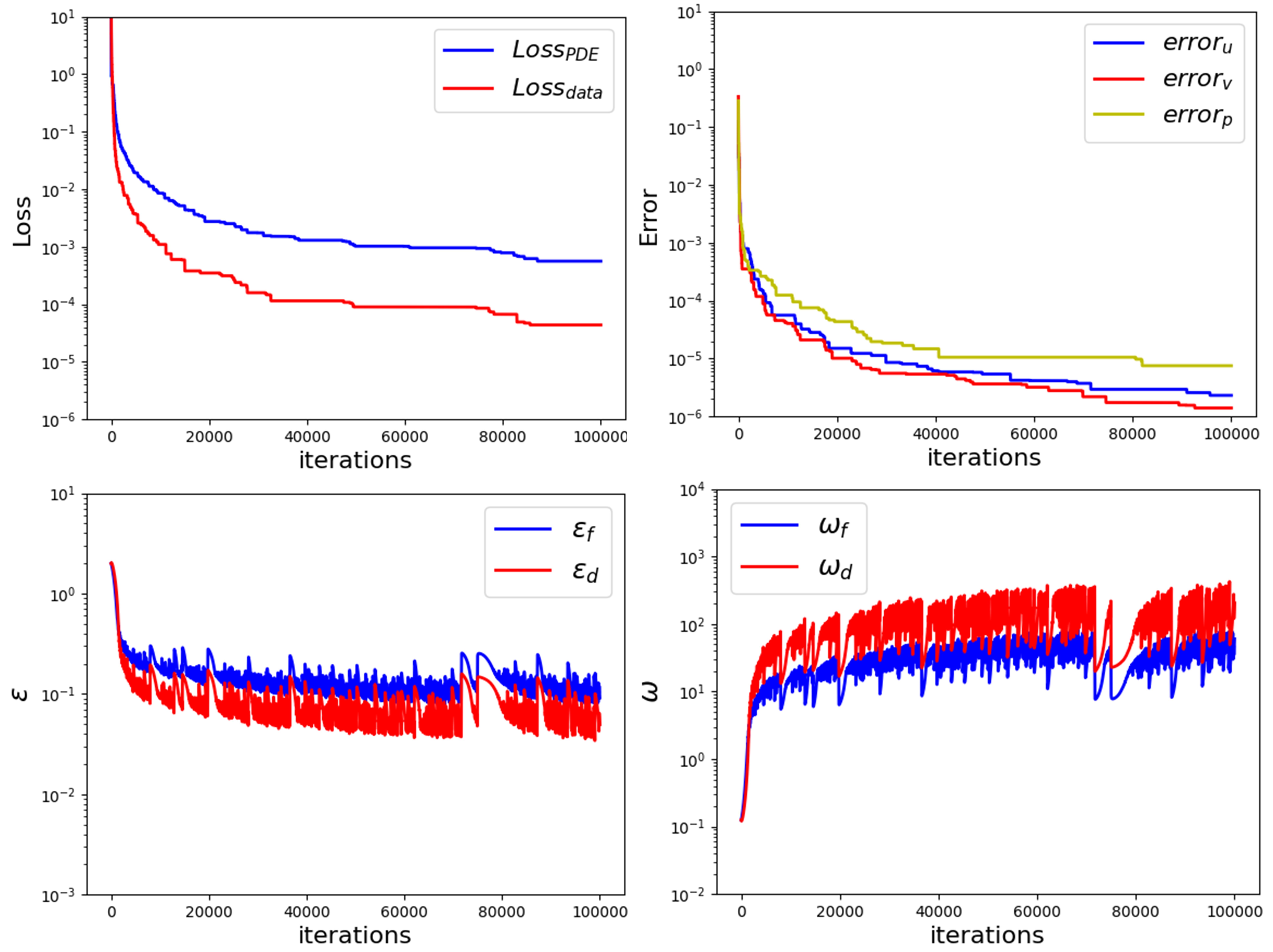
Figure 9: $Loss_{PDE},Loss_{BC},Loss_{data}$, $\varepsilon_{f},\varepsilon_{b},\varepsilon_{d}$, and $\omega_{f},\omega_{b},\omega_{d}$ diagrams for the Navier–Stokes equations are shown. In addition, the convergence of $error_{u},error_{v}$, and $error_{p}$ are displayed.

Table 5: Comparing the error for the velocity and pressure when simulating cylinder wake by PINNs with different weight selections $[\omega_{f},\omega_{d}]$ and lbPINNs with different initial noise configuration $[\varepsilon_{f},\varepsilon_{d}]$.

Methods	parameter selections	$error_{u}$	$error_{v}$	$error_{p}$
PINNs	$[1,1]$	$5.32177e-04$	$3.75389e-04$	$5.26285e-03$
PINNs	$[10,10]$	$2.30731e-04$	$1.70630e-04$	$3.19586e-03$
lbPINNs	$[2,2]$	$4.56425e-06$	$4.81809e-06$	$1.06708e-04$
lbPINNs	$[2,0.04]$	$8.50794e-06$	$6.71318e-06$	$5.37089e-04$

Table 6: Numerical results of Beltrami flow computed by lbPINNs initialized with Similar initial noise settings.

Initial settings	Excellent settings	$Loss_{PDE}$	$Loss_{IC}$	$Loss_{BC}$
$[2,2,2]$	$[2.260e-01,1.171e-01,3.140e-01]$	$1.051e-02$	$1.303e-03$	$1.684e-02$
$[0.2,2,0.2]$	$[3.059e-02,1.481962e-01,3.549e-02]$	$8.286e-02$	$2.796e-02$	$1.151e-02$
$[2,10,2]$	$[2.718e-01,1.705e+00,6.625e-01]$	$2.926e-02$	$3.418e-02$	$1.188e-02$

4.3 Beltrami flow

Applying the proposed algorithm to the three-dimensional Beltrami flow 1994Exact . The 3d unsteady Navier-Stokes flow has the following analytical solution:

$$u(x,y,z,t)= -a\left[e^{ax}\sin(ay+dz)+e^{az}\cos(ax+dy)\right]e^{-d^{2}t},$$ (11)

$$v(x,y,z,t)= -a\left[e^{ay}\sin(az+dx)+e^{ax}\cos(ay+dz)\right]e^{-d^{2}t},$$

$$w(x,y,z,t)= -a\left[e^{az}\sin(ax+dy)+e^{ay}\cos(az+dx)\right]e^{-d^{2}t},$$

$$p(x,y,z,t)= -\frac{1}{2}a^{2}\left[e^{2ax}+e^{2ay}+e^{2az}\right.$$

$$+2\sin(ax+dy)\cos(az+dx)e^{a(y+z)}$$

$$+2\sin(ay+dz)\cos(ax+dy)e^{a(z+x)}$$

$$\left.+2\sin(az+dx)\cos(ay+dz)e^{a(x+y)}\right]e^{-2d^{2}t}$$

where the parameters $a$ and $d$ are 1. The spatial domain is $[-1,1]\times[-1,1]\times[-1,1]$. The time interval is $[0,1]$. For this problem, we study the accuracy of the lbPINN method for the Reynolds number $Re=1$. We fix the network architecture with $layers=10$ and $layersizes=[4,100,100,100,100,100,100,100,100,100,100,4]$. The total numbers of training points are maintained as $N_{b}=100,N_{i}=100$, and $N_{f}=2601$. Besides, the activation function is tanh and then train the network with a learning rate of 0.001 for 5000 epochs by optimizing equation (8). We also present the errors of simulation results of lbPINNs with different initial settings ${\varepsilon_{f},\varepsilon_{i},\varepsilon_{b}}$ in table 6. The final configuration of collection $\varepsilon$ also always achieves $10^{-1}$, which results in the error of PDE residual, boundary, and initial are in the range $10^{-2}\pm 10^{-3}$.

We consider $[\varepsilon_{f},\varepsilon_{i},\varepsilon_{b}]=[2,2,2]$ to its initial settings. In figure 10, the relative absolute errors between the predicted and exact solution of velocity $u(x,y)$, $v(x,y)$, and $w(x,y)$ at a representative time instant on the plane $z=0$ are presented. In addition, we employ lbPINNs to predict the pressure $p(x,y)$ in figure 11. In order to compare clearly, the average error of the velocity and pressure for PINNs and lbPINNs are illustrated in table 7. It is obvious that the predictive error computed with L2 error over 5000 epochs of velocity and pressure could attain $10^{-4}\pm 10^{-5}$, which denominates the high precision of self-adaptive loss balanced method. We further display the curves of $error_{u},error_{v},error_{w}$, and $error_{p}$ in figure 12. The loss, noise constants, and weights number of iterations are also shown. The range of excellent noise parameters is $[2.614\times 10^{-1}\pm 2.260\times 10^{-1},1.965\times 10^{-1}\pm 1.171\times 10^{-1},3.140\times 10^{-1}\pm 3.029\times 10^{-1}]$. The parameter $\varepsilon_{b}$ came down slower than other parameters at the same iterations, which leads to lower $\omega_{b}$ and higher $Loss_{BC}$.

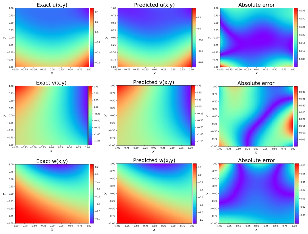
Figure 10: According to temporal snapshots $t=1$ on the plane $z=0$ to compare the exact velocity $u(x,y)$ (Top), $v(x,y)$ (Middle), $w(x,y)$ (Bottom) and predicted solutions of three-dimensional Beltrami flow solved using the self-adaptive loss balance approach.

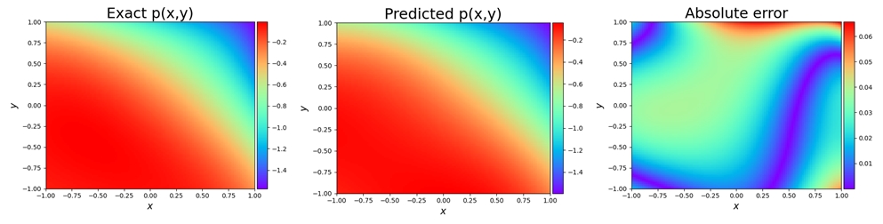
Figure 11: Beltrami flow: analytical solutions and numerical approximations of pressure $p(x,y)$ at $t=1$ on the plane $z=0$ using the developed PINNs.

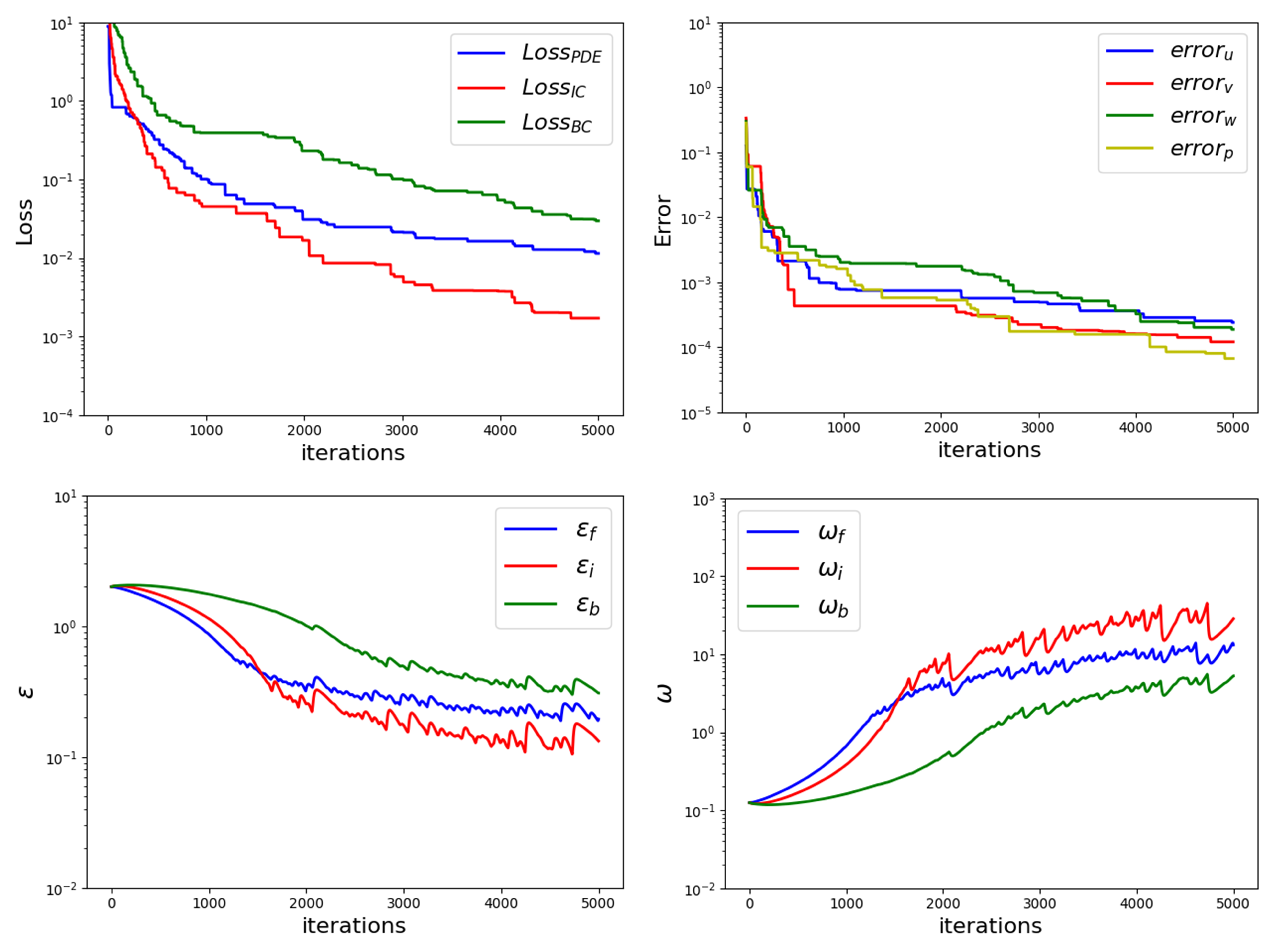
Figure 12: $Loss_{PDE},Loss_{BC}$, $\varepsilon_{f},\varepsilon_{b}$, and $\omega_{f},\omega_{b}$ diagrams for the two-dimensional Kovasznay flow are shown. The curves of $error_{u},error_{v},error_{w}$, and $error_{p}$ are also displayed.

Table 7: Comparing the average absolute error of the velocity and pressure using baseline PINNs with different weight selections $[\omega_{f},\omega_{i},\omega_{b}]$ and lbPINNs with different initial noise configuration $[\varepsilon_{f},\varepsilon_{i},\varepsilon_{b}]$and lbPINNs.

Methods	parameter selections	$error_{u}$	$error_{v}$	$error_{w}$	$error_{p}$
PINNs	$[1,1,1]$	$1.18639e-02$	$2.95078e-03$	$1.39362e-03$	$1.04428e-02$
PINNs	$[20,10,2]$	$7.86194e-03$	$1.64679e-03$	$7.65673e-03$	$9.84695e-02$
lbPINNs	$[2,2,2]$	$3.21078e-04$	$9.90049e-05$	$2.34041e-04$	$1.87083e-04$
lbPINNs	$[2,10,2]$	$1.82803e-04$	$8.64701e-05$	$5.61524e-04$	$1.28763e-04$

5 Conclusions

In this paper, we observe that there exists a competitive relationship between complex physics loss items in PINNs. The performance and convergence of PINNs were susceptible to various loss weight selections. Thus it is beneficial to adaptively assign appropriate weights to combine multiple loss functions in PINNs. We propose a self-adaptive loss balanced method based on maximizing the Gaussian likelihood with the scalable uncertainty parameters to learn these competing loss terms in PINNs simultaneously. The objective of this work is to reconstruct the incompressible Navier-Stokes flows with higher accuracy. The effectiveness and merits of lbPINNs are demonstrated by investigating several laminar flows, including two-dimensional steady Kovasznay flow, two-dimensional unsteady cylinder wake, and three-dimensional unsteady Beltrami flow. Various experimental results could support our claim that the decay of the loss function is slightly faster, and the relative error is lower than that of original PINNs. Moreover, we initialize different sets of uncertainty parameters to indicate the outstanding adaptability of lbPINNs.

The self-adaptive loss balanced Physics-informed neural networks make progress in simulating unsteady Navier-Stokes flow field. However, the noise parameters that play a leading role in weighting loss items are determined by the optimization algorithms for training deep neural networks. To the best of our knowledge, there is no guarantee that gradient-based optimization algorithms would find the exact solution. It is worth attaching importance to theoretical analysis on the phenomenon and improving the robustness and scalability.

References

- (1) S. Boragan Aruoba, Jesus Fernandez-Villaverde, and Juan F. Rubio-Ramirez. Finite elements method. Qm & Rbc Codes, 53(8):1937–1958, 2003.
- (2) Bouchaib Radi and Abdelkhalak El Hami. Finite Volume Methods. John Wiley & Sons, Ltd, 2018.
- (3) Julius O. Smith Iii. Finite difference methods. Polymer Processing, 24(1):385–451, 2009.
- (4) Marta D’Elia, Mauro Perego, and Alessandro Yeneziani. A variational data assimilation procedure for the incompressible navier-stokes equations in hemodynamics. Journal of Scientific Computing, 52(2):340–359, 2012.
- (5) Wang, Jian-Xun, Xiao, and Heng. Data-driven cfd modeling of turbulent flows through complex structures. International Journal of Heat & Fluid Flow, 2016.
- (6) V. Mons, J. C. Chassaing, T. Gomez, and P. Sagaut. Reconstruction of unsteady viscous flows using data assimilation schemes. Journal of Computational Physics, pages 255–280, 2016.
- (7) Sean Symon, Nicolas Dovetta, Beverley J. McKeon, Denis Sipp, and Peter J. Schmid. Data assimilation of mean velocity from 2d piv measurements of flow over an idealized airfoil. Experiments in Fluids, 2017.
- (8) Jian Yu and Jan S Hesthaven. Flowfield reconstruction method using artificial neural network. AIAA Journal, 57(2):482–498, 2019.
- (9) Shaoxing Mo, Nicholas Zabaras, Xiaoqing Shi, and Jichun Wu. Deep autoregressive neural networks for high-dimensional inverse problems in groundwater contaminant source identification. 2018.
- (10) Chao Jiang, Junyi Mi, Shujin Laima, and Hui Li. A novel algebraic stress model with machine- learning-assisted parameterization. Energies, 13:258, 01 2020.
- (11) Zhideng Zhou, Guowei He, Shizhao Wang, and Guodong Jin. Subgrid-scale model for large-eddy simulation of isotropic turbulent flows using an artificial neural network. Computers & Fluids, 195:104319, 2019.
- (12) Yang Liu, Nam Dinh, Yohei Sato, and Bojan Niceno. Data-driven modeling for boiling heat transfer: using deep neural networks and high-fidelity simulation results, 06 2018.
- (13) Isaac Elias Lagaris, Aristidis C. Likas, and Dimitrios G. Papageorgiou. Neural-network methods for boundary value problems with irregular boundaries. IEEE Transactions on Neural Networks, 11(5):1041–9, 2000.
- (14) Maziar Raissi, Alireza Yazdani, and George Karniadakis. Hidden fluid mechanics: A navier-stokes informed deep learning framework for assimilating flow visualization data, 08 2018.
- (15) Guofei Pang and George Em Karniadakis. Physics-Informed Learning Machines for Partial Differential Equations: Gaussian Processes Versus Neural Networks. 2020.
- (16) Maziar Raissi. Deep hidden physics models: Deep learning of nonlinear partial differential equations. Journal of Machine Learning Research, 2018.
- (17) Liu Yang, Dongkun Zhang, and George Em Karniadakis. Physics-informed generative adversarial networks for stochastic differential equations, 2018.
- (18) Maziar Raissi, Paris Perdikaris, and George Em Karniadakis. Physics informed deep learning (part i): Data-driven solutions of nonlinear partial differential equations, 2017.
- (19) Maziar Raissi, Paris Perdikaris, and George E Karniadakis. Physics-informed neural networks: A deep learning framework for solving forward and inverse problems involving nonlinear partial differential equations. Journal of Computational Physics, 378:686–707, 2019.
- (20) Daniel E Hurtado, Francisco Sahli Costabal, Yibo Yang, Paris Perdikaris, and Ellen Kuhl. Physics-informed neural networks for cardiac activation mapping. Frontiers of Physics, 8(42), 2020.
- (21) Kathrin Glau and Linus Wunderlich. The deep parametric pde method: Application to option pricing. Papers, 2020.
- (22) Atilim Gunes Baydin, Barak A. Pearlmutter, Alexey Andreyevich Radul, and Jeffrey Mark Siskind. Automatic differentiation in machine learning: a survey. 2015.
- (23) Ryan King, Oliver Hennigh, Arvind Mohan, and Michael Chertkov. From deep to physics-informed learning of turbulence: Diagnostics, 10 2018.
- (24) Xiang Yang, Suhaib Zafar, Jian-Xun Wang, and Heng Xiao. Predictive large-eddy-simulation wall modeling via physics-informed neural networks. Physical Review Fluids, 4, 03 2019.
- (25) Qizhi He and Alexandre Tartakovsky. Physics-informed neural network method for forward and backward advection-dispersion equations, 12 2020.
- (26) Xiaowei Jin, Shengze Cai, Hui Li, and George Em Karniadakis. Nsfnets (navier-stokes flow nets): Physics-informed neural networks for the incompressible navier-stokes equations. 2020.
- (27) Zhiping Mao, Ameya Jagtap, and George Karniadakis. Physics-informed neural networks for high-speed flows. Computer Methods in Applied Mechanics and Engineering, 03 2020.
- (28) Luning Sun, Han Gao, Shaowu Pan, and Jian Xun Wang. Surrogate modeling for fluid flows based on physics-constrained deep learning without simulation data. Computer Methods in Applied Mechanics and Engineering, 361.
- (29) Moloud Abdar, Farhad Pourpanah, Sadiq Hussain, Dana Rezazadegan, Li Liu, Mohammad Ghavamzadeh, Paul Fieguth, Xiaochun Cao, Abbas Khosravi, U Rajendra Acharya, Vladimir Makarenkov, and Saeid Nahavandi. A review of uncertainty quantification in deep learning: Techniques, applications and challenges, 2020.
- (30) Luning Sun and Jian Xun Wang. Physics-constrained bayesian neural network for fluid flow reconstruction with sparse and noisy data. Theoretical & Applied Mechanics Letters, v.10(03):28–36, 2020.
- (31) Yinhao Zhu, Nicholas Zabaras, Phaedon Stelios Koutsourelakis, and Paris Perdikaris. Physics-constrained deep learning for high-dimensional surrogate modeling and uncertainty quantification without labeled data. Journal of Computational Physics, 394:56–81, 2019.
- (32) Shengze Cai, Zhicheng Wang, Chryssostomos Chryssostomidis, and George Karniadakis. Heat transfer prediction with unknown thermal boundary conditions using physics-informed neural networks. 07 2020.
- (33) Chiyuan Zhang, Qianli Liao, Alexander Rakhlin, Brando Miranda, Noah Golowich, and Tomaso A. Poggio. Theory of deep learning iib: Optimization properties of SGD. CoRR, abs/1801.02254, 2018.
- (34) Diederik Kingma and Jimmy Ba. Adam: A method for stochastic optimization. Computer ence, 2014.
- (35) Sergios Theodoridis. Stochastic gradient descent. Machine Learning, pages 161–231, 2015.
- (36) Mohannad Elhamod, Jie Bu, Christopher Singh, Matthew Redell, Abantika Ghosh, Viktor Podolskiy, Wei-Cheng Lee, and Anuj Karpatne. Cophy-pgnn: Learning physics-guided neural networks withcompeting loss functions for solving eigenvalue problems, 2020.
- (37) Sifan Wang, Xinling Yu, and Paris Perdikaris. When and why pinns fail to train: A neural tangent kernel perspective, 07 2020.
- (38) Sifan Wang, Yujun Teng, and Paris Perdikaris. Understanding and mitigating gradient pathologies in physics-informed neural networks, 2020.
- (39) Levi McClenny and Ulisses Braga-Neto. Self-adaptive physics-informed neural networks using a soft attention mechanism, 09 2020.
- (40) Alex Kendall, Yarin Gal, and Roberto Cipolla. Multi-task learning using uncertainty to weigh losses for scene geometry and semantics, 2018.
- (41) Xiaoli Chen, Liu Yang, Jinqiao Duan, and George Em Karniadakis. Solving inverse stochastic problems from discrete particle observations using the fokker-planck equation and physics-informed neural networks. 2020.
- (42) Maziar Raissi. Forward-backward stochastic neural networks: Deep learning of high-dimensional partial differential equations. 2018.
- (43) Dongkun Zhang, Ling Guo, and George Em Karniadakis. Learning in modal space: Solving time-dependent stochastic pdes using physics-informed neural networks. 2019.
- (44) Dongkun Zhang, Lu Lu, Ling Guo, and George Em Karniadakis. Quantifying total uncertainty in physics-informed neural networks for solving forward and inverse stochastic problems. Journal of Computational Physics, 2019.
- (45) Guofei Pang, Lu Lu, and George Em Karniadakis. fpinns: Fractional physics-informed neural networks, 2018.
- (46) Colby L. Wight and Jia Zhao. Solving allen-cahn and cahn-hilliard equations using the adaptive physics informed neural networks, 2020.
- (47) Yeonjong Shin, Jerome Darbon, and George Em Karniadakis. On the convergence and generalization of physics informed neural networks. 2020.
- (48) Matthew Tancik, Pratul P. Srinivasan, Ben Mildenhall, Sara Fridovich-Keil, Nithin Raghavan, Utkarsh Singhal, Ravi Ramamoorthi, Jonathan T. Barron, and Ren Ng. Fourier features let networks learn high frequency functions in low dimensional domains. 2020.
- (49) Justin Sirignano and Konstantinos Spiliopoulos. Dgm: A deep learning algorithm for solving partial differential equations. JCoPh, 375, 2018.
- (50) Vincent Sitzmann, Julien N. P Martel, Alexander W Bergman, David B Lindell, and Gordon Wetzstein. Implicit neural representations with periodic activation functions. 2020.
- (51) Chigozie Nwankpa, Winifred Ijomah, Anthony Gachagan, and Stephen Marshall. Activation functions: Comparison of trends in practice and research for deep learning. 2018.
- (52) Prajit Ramachandran, Barret Zoph, and Quoc V. Le. Searching for activation functions. 2017.
- (53) Alex Kendall and Yarin Gal. What uncertainties do we need in bayesian deep learning for computer vision?, 2017.
- (54) S. Dong and J. Shen. An unconditionally stable rotational velocity-correction scheme for incompressible flows. Journal of Computational Physics, 229(19):7013–7029, 2010.
- (55) C. Ross Ethier and D. A. Steinman. Exact fully 3d navier–stokes solutions for benchmarking. International Journal for Numerical Methods in Fluids, 19, 1994.