Fairness in Rankings and Recommendations: An Overview

Abstract

We increasingly depend on a variety of data-driven algorithmic systems to assist us in many aspects of life. Search engines and recommender systems amongst others are used as sources of information and to help us in making all sort of decisions from selecting restaurants and books, to choosing friends and careers. This has given rise to important concerns regarding the fairness of such systems. In this work, we aim at presenting a toolkit of definitions, models and methods used for ensuring fairness in rankings and recommendations. Our objectives are three-fold: (a) to provide a solid framework on a novel, quickly evolving, and impactful domain, (b) to present related methods and put them into perspective, and (c) to highlight open challenges and research paths for future work.

1 Introduction

Algorithmic systems, driven by large amounts of data, are increasingly being used in all aspects of society to assist people in forming opinions and taking decisions. Such algorithmic systems offer enormous opportunities, since they accelerate scientific discovery in various domains, including personalized medicine, smart weather forecasting and many other fields. They can also automate tasks regarding simple personal decisions, and help in improving our daily life through personal assistants and recommendations, like where to eat and what are the news. Moving forward, they have the potential of transforming society through open government and many more benefits.

Often, such systems are used to assist, or, even replace human decision making in diverse domains. Examples include software systems used in school admissions, housing, pricing of goods and services, credit score estimation, job applicant selection, and sentencing decisions in courts and surveillance. This automation raises concerns about how much we can trust such systems.

A steady stream of studies has shown that decision support systems can unintentionally both encode existing human biases and introduce new ones DBLP:journals/cacm/ChouldechovaR20 . For example, in image search, when the query is about doctors or nurses, what is the percentage of images portraying women that we get in the result? Evidence shows stereotype exaggeration and systematic underrepresentation of women when compared with the actual percentage, as estimated by the US Bureau of labor and statistics DBLP:conf/chi/KayMM15 . Two interesting conclusions from the study were that people prefer and rate search results higher when these results are consistent with stereotypes. Another interesting result is that if you shift the representation of gender in image search results then the people’s perception about real world distribution tends to shift too.

Another well-known example is the COMPAS system, which is a commercial tool that uses a risk assessment algorithm to predict some categories of future crime. Specifically, this tool is used in courts in the US to assist bail and sentencing decisions, and it was found that the false positive rate, that is the people who were labeled by the tool as high risk but did not re-offend, was nearly twice as high for African-American as for white defendants Angwin16 . This means that many times the ubiquitous use of decision support systems may create possible threats of economic loss, social stigmatization, or even loss of liberty. There are many more case studies, like the above ones. For example, names that are used by men and women of color are much more likely to generate ads related to arrest records DBLP:journals/cacm/Sweeney13 . Also using a tool called Adfisher, it was found that if you set the gender to female, this will result in getting ads for less high paid jobs. Or, in the case of word embeddings the vector that represents computer programming is closer to men than to women.

Data-driven systems are also being employed by search and recommendation engines in movie and music platforms, advertisements, social media, and news outlets, among others. Recent studies report that social media has become the main source of online news with more than 2.4 billion internet users, of which nearly 64.5% receive breaking news from social media instead of traditional sources martin18 . Thus, to a great extent, search and recommendation engines in such systems play a central role in shaping our experiences and influencing our perception of the world.

For example, people come to their musical tastes in all kinds of ways, but how most of us listen to music now offers specific problems of embedded bias. When a streaming service offers music recommendations, it does so by studying what music has been listened to before. That creates a suggestions loop, amplifying existing bias and reducing diversity. A recent study analysed the publicly available listening records of 330,000 users of one service and showed that female artists only represented 25 per cent of the music listened to by users. The study identified that gender fairness is one of the artists’ main concerns as female artists are not given equal exposure in music recommendations DBLP:conf/chiir/FerraroSB21 .

Another study led by University of Southern California on Facebook ad recommendations revealed that the recommendation system disproportionately showed certain types of job ads to men and women Imana21a . The system was more likely to present job ads to users if their gender identity reflected the concentration of that gender in a particular position or industry. Hence, recommendations amplified existing bias and created fewer opportunities for people based on their gender. However, ads may be targeted based on qualifications, but not on protected categories, based on US law.

In this article, we pay special attention to the concept of fairness in rankings and recommendations. By fairness, we typically mean lack of discrimination (bias). Bias may come from the algorithm, reflecting, for example, commercial or other preferences of its designers, or even from the actual data, for example, if a survey contains biased questions, or, if some specific population is misrepresented in the input data.

As fairness is an elusive concept, an abundance of definitions and models of fairness have been proposed as well as several algorithmic approaches for fair rankings and recommendations making the landscape very convoluted. In order to make real progress in building fair-aware systems, we need to de-mystify what has been done, understand how and when each model and approach can be used, and, finally, distinguish the research challenges ahead of us.

Therefore, we follow a systematic and structured approach to explain the various sides of and approaches to fairness. In this survey, we present fairness models for rankings and recommendations separately from the computational methods used to enforce them, since many of the computational methods originally introduced for a specific model are applicable to other models as well. By providing an overview of the spectrum of different models and computational methods, new ways to combine them may evolve.

We start by presenting fairness models. First, we provide a birds’ eye view of how notions of fairness in rankings and recommendations have been formalized. We also present a taxonomy. Specifically, we distinguish between individual and group fairness, consumer and producer fairness, and fairness for single and multiple outputs. Then, we present concrete models and definitions for rankings and recommendations. We highlight their differences and commonalities, and present how these models fit into our taxonomy.

We describe solutions for fair rankings and recommendations. We organize them into pre-processing approaches that aim at transforming the data to remove any underlying bias or discrimination, in-processing approaches that aim at modifying existing or introducing new algorithms that result in fair rankings and recommendations, and post-processing approaches that modify the output of the algorithm. Within each category, we further classify approaches along several dimensions. We discuss other cases where a system needs to make decisions and where fairness is also important, and present open research challenges pertaining to fairness in the broader context of data management.

To the best of our knowledge, this is the first survey that provides a toolkit of definitions, models and methods used for ensuring fairness in rankings and recommendations. A recent survey focuses on fairness in ranking DBLP:journals/corr/abs-2103-14000 . The two surveys are complementary to each other both in terms of perspective and in terms of coverage. Fairness is an evasive concept and integrating it in algorithms and systems is an emerging fast-changing field. We provide a more technical classification of recent work, whereas the view in DBLP:journals/corr/abs-2103-14000 is a socio-technical one that aims at placing the various approaches to fairness within a value framework. Content is different as well, since we also cover recommendations and rank aggregation. Recent tutorials, with a stricter focus than ours, focusing on concepts and metrics of fairness and the challenges in applying these to recommendations and information retrieval, as well as to scoring methods, are presented, respectively, in DBLP:conf/sigir/EkstrandBD19 and DBLP:journals/pvldb/AsudehJ20 ; DBLP:conf/www/OosterhuisJR20 . On the other hand, this article has a much wider coverage and depth, presenting a structured survey and comparison of methods and models for ensuring fairness in rankings and recommendations.

The remaining of this survey is organized as follows. Section 2 presents the core definitions of fairness, and Section 3 reviews definitions of fairness that are applicable specifically to rankings, recommenders and rank aggregation. Section 4 discusses a distinction of the methods for achieving fairness, while Sections 5, 6 and 7 organize and present in detail the pre-, in- and post-processing methods. Section 8 offers a comparison between the in- and post-processing methods. Section 9 studies how we can verify whether a program is fair. Finally, Section 10 elaborates on critical open issues and challenges for future work, and Section 11 summarizes the status of the current research on fairness in ranking and recommender systems.

2 The Fairness Problem

In this section, we start with an overview of approaches to modeling fairness and then provide a taxonomy of the different types of fairness models in ranking and recommendations.

2.1 A General View on Fairness

Most approaches to algorithmic fairness interpret fairness as lack of discrimination DBLP:journals/corr/FriedlerSV16 ; DBLP:journals/cacm/FriedlerSV21 , asking that an algorithm should not discriminate against its input entities based on attributes that are not relevant to the task at hand. Such attributes are called protected, or sensitive, and often include among others gender, religion, age, sexual orientation, and race.

So far, most work on defining, detecting and removing unfairness has focused on classification algorithms used in decision making. In classification algorithms, each input entity is assigned to one from a set of predefined classes. In this case, characteristics of the input entities that are not relevant to the task at hand should not influence the output of the classifier. For example, the values of protected attributes should not hinder the assignment of an entity to the positive class, where the positive class may for example, correspond to getting a job, or, being admitted at a school.

In this paper, we focus on ranking and recommendation algorithms. Given a set of entities, $\{i_{1},i_{2},\dots i_{N}\}$, a ranking algorithm produces a ranking $r$ of the entities, where $r$ is an assignment (mapping) of entities to ranking positions. Ranking is based on some measure of the relative quality of the entities for the task at hand. For example, the entities in the output of a search query are ranked mainly based on their relevance to the query. In the following, we will also refer to the measure of quality, as utility. Abstractly, a fair ranking is one where the assignment of entities to positions is not unjustifiably influenced by the values of their protected attributes.

Recommendation systems retrieve interesting items for users based on their profiles and their history. Depending on the application and the recommendation system, history may include explicit user ratings of items, or, selection of items (e.g., views, clicks). In general, recommenders estimate a score, or, rating, $\hat{s}(u,i)$ for a user $u$ and an item $i$ that reflects the preference of user $u$ for item $i$, or, in other words, the relevance of item $i$ for user $u$. Then, a recommendation list $I$ is formed for user $u$ that includes the items having the highest estimated score for $u$. These scores can be seen as the utility scores in the case of recommenders. In abstract terms, a recommendation is fair, if the values of the protected attributes of the users, or, the items, do not affect the outcome of the recommendation.

On a high level, we can distinguish between two approaches to formalizing fairness DHP+12 :

• Individual fairness definitions are based on the premise that similar entities should be treated similarly.

• Group fairness definitions group entities based on the value of one or more protected attributes and ask that all groups are treated similarly.

To operationalize both approaches to fairness, we need to define similarity for the input and the output of an algorithm. For input similarity, we need a means of quantifying similarity of entities in the case of individual fairness, and, a way of partitioning entities into groups, in the case of group fairness. For output similarity, for both individual and group fairness, we need a formal definition of what similar treatment means.

Input similarity. For individual fairness, a common approach to defining input similarity is a distance-based one DHP+12 . Let $V$ be the set of entities, we assume there is a distance metric $d:V\times V\rightarrow R$ between each pair of entities, such that, the more dissimilar the entities, the larger their distance. This metric should be task-specific, that is, two entities may be similar for one task and dissimilar for another. For example, two individuals may be consider similar to each other (e.g., have similar qualifications) when it comes to being admitted to college but dissimilar when it comes to receiving a loan. The metric may be externally imposed, e.g., by a regulatory body, or externally proposed, e.g., by a civil rights organization. Ideally, the metric should express the ground truth, or, the best available approximation of it. Finally, this metric should be made public, and open to discussion and refinement. For group fairness, the challenge lies in determining how to partition entities into groups.

Output similarity. Specifying what it means for entities, or groups of entities to be treated similarly is an intricate problem, from both a social and a technical perspective. From a social perspective, a fundamental distinction is made between equity and equality. Simply put, equality refers to treating entities equally, while equity refers to treating entities according to their needs, so that they all finally receive the same output, even when some individuals are disadvantaged.

Note that, often blindness, i.e., hiding the values of the protected attributes, does not suffice to produce fair outputs, since there may be other proxy attributes correlated with the protected ones, a case also known as redundant encoding. Take for example a zip code attribute. Zip codes may reveal sensitive information when the majority of the residents of a neighborhood belong to a specific ethnic group redlining . In fact, such considerations have led to making redlining, i.e., the practice of arbitrary denying or limiting financial services to specific neighborhoods, illegal in the US.

Another social-based differentiation can be made between disparate treatment and disparate impact. Disparate treatment is the often illegal practice of treating an entity differently based on its protected attributes. Disparate impact refers to cases where the output depends on the protected attributes, even if all entities are treated the same way. The disparate impact doctrine was solidified in the US after [Griggs v. Duke Power Co. 1971] where a high school diploma was required for unskilled work, excluding applicants of color.

From a technical perspective, how output similarity is translated into quantifiable measures depends clearly on the specific type of algorithm. In this paper, we focus on ranking and recommendation algorithms.

Overall, in the case of ranking, a central issue is the manifestation of position bias, i.e., the fact that people tend to consider only the items that appear in the top few positions of a ranking. Even more the attention that items receive, that is the visibility of the items, is highly skewed with regards to their position in the list. At a high level, output similarity in the case of ranking refers to offering similar visibility to similar items or group of items, that is, placing them at similar positions in the ranking, especially when it comes to top positions.

For recommendations, one approach to defining output fairness is to consider the recommendation problem as a classification problem where the positive class is the recommendation list. Another approach is to consider the recommendation list $I$ as a ranked list $r$, in which case, the position of each recommended item in the list should also be taken into account.

We refine individual and group fairness based on the type of output similarity in the next section.

2.2 A Taxonomy of Fairness Definitions

In the previous section, we distinguished between individual and group fairness formulations. We will refer to this distinction of fairness models as the level of fairness. When it comes to ranking and recommendation systems, besides different levels, we also have more than one side at which fairness criteria are applicable. Finally, we differentiate fairness models based on whether the fairness requirements are applied at a single or at multiple outputs of an algorithm. The different dimensions of fairness are summarized in Figure 1.

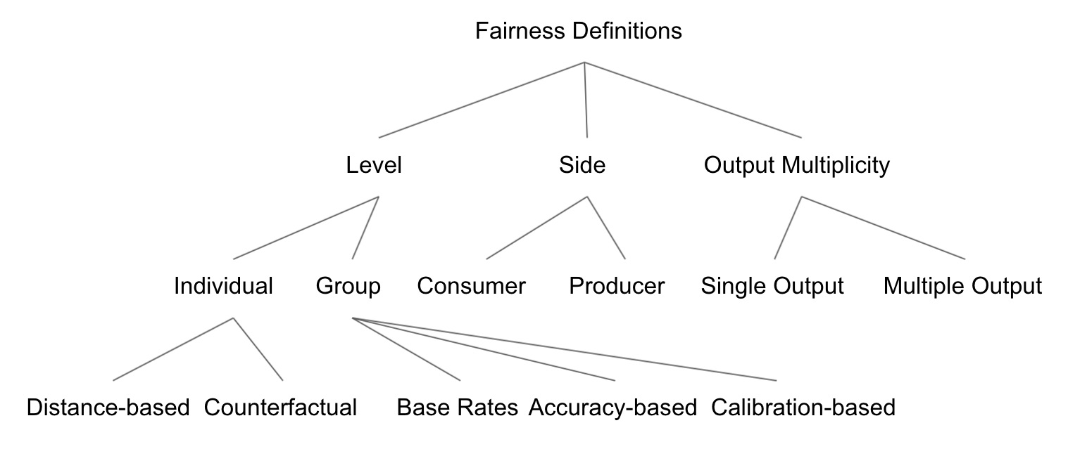
Figure 1: Fairness Definitions Taxonomy.

Note, that the various fairness definitions in this and the following sections can be used both: (a) as conditions that a system must satisfy for being fair, and (b) as measures of fairness. For instance, we can measure how much a fairness condition is violated, or, define a condition by setting a threshold on a fairness measure.

2.2.1 Levels of fairness

We now refine individual and group fairness based on how output similarity is specified. Seminal research in formalizing algorithmic fairness has focused on classification algorithms used in decision making. Such research has been influential in the study of fairness in other types of algorithms. So, we refer to such research briefly here and relate it to ranking and recommendations.

Types of Individual Fairness. One way of formulating individual fairness is a distance-based one. Intuitively, given a distance measure $d$ between two entities, and a distance measure $D$ between the outputs of an algorithm, we would like the distance between the output of the algorithm for two entities to be small, when the entities are similar. Let us see a concrete example from the area of probabilistic classifiers DHP+12 .

Let $M$ be a classifier that maps entities $V$ to outcomes $A$. In the case of probabilistic classifiers, these are randomized mappings from entities to probability distributions over outcomes. Specifically, to classify an entity $v\in V$, we choose an outcome $a\in A$ according to the distribution $M(v)$. We say that a classifier is individually fair if the mapping $M:$ $V\rightarrow\Delta(A)$ satisfies the $(D,d)$-Lipschitz property, that is, $\forall\,v,u\in V$, $D(M(v),M(u))\leq d(v,u)$, where $D$ is a distance measure between probability distributions, and $d$ a distance metric between entities. In words, the distance $D$ between probability distributions assigned by the classifier $M$ should be no greater than the actual distance $d$ between the entities.

Another form of individual fairness is counterfactual fairness KLR+17 . The intuition in this case, is that an output is fair towards an entity if it is the same in both the actual world and a counterfactual world where the entity belonged to a different group. Causal inference is used to formalize this notion of fairness.

Types of Group Fairness. For simplicity, let us assume two groups, namely, the protected group $G^{+}$ and the non-protected (or, privileged) group $G^{-}$. We will start by presenting statistical approaches commonly used in classification. Assume that $Y$ is the actual and $\hat{Y}$ the predicted output of a binary classifier, that is, $Y$ is the ground truth, and $\hat{Y}$ the output of the algorithm. Let $1$ be the positive class that leads to a favorable decision, e.g., someone getting a loan, or being admitted at a competitive school, and $S$ be the predicted probability for a certain classification.

Statistical approaches to group fairness can be distinguished as FSV+19 ; VR18 :

• base rates approaches: that use only the output $\hat{Y}$ of the algorithm,

• accuracy approaches: that use both the output $\hat{Y}$ of the algorithm and the ground truth $Y$, and

• calibration approaches: that use the predicted probability $S$ and the ground truth $Y$.

In classification, base rate fairness compares the probability $P(\hat{Y}=1|v\in G^{+})$ that an entity $v$ receives the favorable outcome when $v$ belongs to the protected group $G^{+}$ with the corresponding probability $P(\hat{Y}=1|v\in G^{-})$ that $v$ receives the favorable outcome when $v$ belongs to the non-protected group $G^{-}$. To compare the two, we may take their ratio ZWS+13 , FFM+15 : $\frac{P(\hat{Y}=1|v\in G^{+})}{P(\hat{Y}=1|v\in G^{-})}$ or, their difference CV10 : $1-(P(\hat{Y}=1|v\in G^{+})-P(\hat{Y}=1|v\in G^{-}))$.

Now, in abstract terms, a base rate fairness definition for ranking may compare the probabilities of items from each group to appear in similarly good ranking positions, while for recommendations, the probabilities of them being recommended.

When the probabilities of a favorable outcome are equal for the two groups, we have a special type of fairness termed demographic, or statistical parity. Statistical parity preserves the input ratio, that is, the demographics of the individuals receiving a favorable outcome are the same as the demographics of the underlying population. Statistical parity is a natural way to model equity: members of each group have the same chance of receiving the favorable output.

Base rate fairness ignores the actual output, the output may be fair, but it may not reflect the ground truth. For example, assume that the classification task is getting or not a job and the protected attribute is gender. Statistical parity asks for a specific ratio of women in the positive class, even when there are not that many women in the input who are well-qualified for the job. Accuracy and calibration look at traditional evaluation measures and require that the algorithm works equally well in terms of prediction errors for both groups.

In classification, accuracy-based fairness warrants that various types of classification errors (e.g., true positives, false positives) are equal across groups. Depending on the type of classification errors considered, the achieved type of fairness takes different names HPS16 . For example, the case in which, we ask that $P(\hat{Y}=1|Y=1,v\in G^{+})$ = $P(\hat{Y}=1|Y=1,v\in G^{-})$ (i.e., the case of equal true positive rate for the two groups) is called equal opportunity.

Comparing equal opportunity with statistical parity, again the members of the two groups have the same chance of getting the favorable outcome, but only when these members qualify. Thus, equal opportunity is more close to an equality interpretation of fairness.

In analogy to accuracy, in the case of ranking, the ground truth is reflected in the utility of the items. Thus, approaches that take into account utility when defining fairness in ranking can be seen as accuracy-based ones. In recommendations, accuracy-based definitions look at the differences between the actual and the predicted ratings of the items for the two groups.

Calibration-based fairness considers probabilistic classifiers that predict a probability for each class Ch17 ; KMR17 . In general, a classification algorithm is considered to be well-calibrated if: when the algorithm predicts a set of individuals as having probability $p$ of belonging to the positive class, then approximately a $p$ fraction of this set are actual members of the positive class. In terms of fairness, intuitively, we would like the classifier to be equally well-calibrated for both groups. An example calibration-based fairness is asking that for any predicted probability score $p$ in $[0,1]$, the probability of actually getting a favorable outcome is equal for both groups, i.e., $P(Y=1|S=p,v\in G^{+})$ = $P(Y=1|S=p,v\in G^{-})$.

Group-based measures in general tend to ignore the merits of each individual in the group. Some individuals in a group may be better for a given task than other individuals in the group, which is not captured by some group-based fairness definitions. This issue may lead to two problematic behaviors, namely, (a) the self-fulfilling prophecy where by deliberately choosing the less qualified members of the protected group we aim at building a bad track record for the group and (b) reverse tokenism where by not choosing a well qualified member of the non-protected group we aim at creating convincing refutations for the members of the protected group that are also not selected.

2.2.2 Multi-sided fairness

In ranking and recommendations, there are at least two sides involved: the items that are being ranked, or recommended, and the users that receive the rankings or the recommendations. We distinguish between producer or item-side fairness and consumer or user-side fairness. Note that the items that are being ranked or recommended may be also people, for example, in case of ranking job applicants, but we call them items for simplicity.

Producer or item-side fairness focuses on the items that are being ranked, or recommended. In this case, we would like similar items or groups of items to be ranked, or, be recommended in a similar way, e.g., to appear in similar positions in a ranking. This is the main type of fairness, we have discussed so far. For instance, if we consider political orientation as the protected attribute of an article, we may ask that the value of this attribute does not affect the ranking of articles in a search result, or a news feed.

Consumer or user-side fairness focuses on the users who receive, or consume the data items in a ranking, e.g., a search result, or a recommendation. In abstract terms, we would like similar users, or groups of users, to receive similar rankings or recommendations. For instance, if gender is the protected attribute of a user receiving job recommendations, we may ask that the gender of the user does not influence the job recommendations that the user receives.

There are cases in which a system may require fairness for both consumers and providers, when for instance both the users and the items belong to protected groups. For example, assume a rental property business that wishes to treat minority applicants as a protected class and ensure that they have access to properties similar to other renters, while at the same time, wishes to treat minority landlords as a protected class and ensure that highly qualified tenants are referred to them at the same rate as to other landlords.

Different types of recommendation systems may call for specializations of consumer and producer fairness. Such a case is group recommendation systems. Group recommendation systems recommend items to groups of users as opposed to a single user, for example a movie to a group of friends, an event to an online community, or a excursion to a group of tourists grouprec1 ; grouprec2 . In this case, we have different types of consumer fairness, since now the consumer is not just a single user. Another case are bundle and package recommendation systems that recommend complex items, or sets of items, instead of just a single item, for example a set of places to visit, or courses to attend packagerec1 . In this case, we may have different types of producer fairness, since now the recommended items are composite. We discuss these special types of fairness in Section 3.3.

We can expand the sides of fairness further by considering the additional stakeholders that may be involved in a recommendation system besides the consumers and the producers. For example, in a recommendation system, the items being recommended may belong to different providers. For instance, in the case of movie recommendations, the movies may be produced by different studios. In this case, we may ask for producer fairness with respect to the providers of the items, instead of the single items. For example, in an online craft marketplace, we may want to ensure market diversity and avoid monopoly domination, where the system wishes to ensure that new entrants to the market get a reasonable share of recommendations even though they have fewer shoppers than established vendors. Note that one way to model provider fairness is by treating the provider as a protected attribute of the items.

Other sides of fairness include: (a) fairness for the owners of the recommendation system, especially when the owners are different than the producers, and (b) fairness for system regulators and auditors, for example, data scientists, machine learning researchers, policymakers and governmental auditors that are using the system for decision making.

2.2.3 Output Multiplicity

There are may be cases in which it is not feasible to achieve fairness by considering just a single ranking or a single recommendation output. Thus, recently, there exist approaches that propose achieving fairness via a series of outputs. Consider, for example, the case where the same items appear in the results of multiple search queries, or the same users receive more than one recommendation. In such cases, we may ask that an item is not necessarily being treated fairly in each and every search result but the item is treated fairly overall in a set of a search results. Similarly, a user may be treated unfairly in a single recommendation but fairly in a sequence of recommendations.

Concretely, we distinguish between single output and multiple output fairness. In multiple output fairness, we ask for eventual, or amortized consumer, or producer fairness, i.e., we ask that the consumers or producers are treated fairly in a series of rankings or recommendations as a whole, although they may be treated unfairly in one or more single ranking or recommendation in the series.

Another case is sequential recommenders that suggest items of interest by modeling the sequential dependencies over the user-item interactions in a sequence. This means that the recommender treats the user-item interactions as a dynamic sequence and takes the sequential dependencies into account to capture the current and previous user preferences for increasing the quality of recommendations DBLP:conf/sac/StratigiNPS20 . The system recommends different items at each interaction, while retaining knowledge from past interactions. Interestingly, due to the multiple user-item interactions in sequential recommender systems, fairness correction can be performed, while moving from one interaction to the next.

3 Models of Fairness

In the previous section, we presented an overview of fairness and its various dimensions in ranking and recommendations. In this section, we present a number of concrete models and definitions of fairness proposed for ranking, recommendations and rank aggregation.

3.1 Fairness in Rankings

Most approaches to fairness in ranking handle producer fairness, that is, their goal is to ensure that the items being ranked are treated fairly. In general, ranking fairness asks that similar items or group of items receive similar visibility, that is, they appear at similar positions in the ranking. A main issue is accounting for position bias. Since in western cultures, we read from top to bottom and from left to right, the visibility of lower-ranked items drops rapidly when compared to the visibility of higher-ranked ones ricardo .

We will use the example rankings in Figure 2(c). The protected attribute is color, red is the protected group and score is the utility of the item. The ranking on the left ($r_{l}$) corresponds to a ranking based solely on utility, the ranking in the middle ($r_{m}$) achieves the highest possible representation of the protected group in the top positions, while the ranking in the right ($r_{r}$) is an intermediate one.

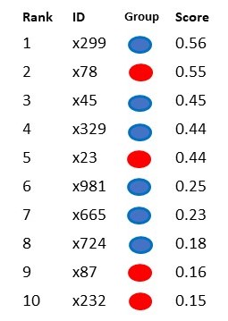
(a) $r_{l}$

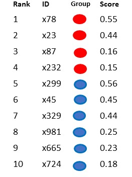
(b) $r_{m}$

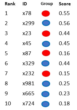
(c) $r_{r}$

Figure 2: Example rankings: (a) $r_{l}$ is based solely on utility, (b) $r_{m}$ is the optimal ranking in terms of the representation of the protected group, (c) $r_{r}$ is an intermediate ranking between the two. Red is the protected value.

Fairness constraints. A number of group-based fairness models for ranking focus on the representation (i.e., number of items) of the protected group in the top-$k$ position in the ranking. One such type of group fairness is achieved by constraining the number of items from the different groups that can appear in the top-$k$ positions. Specifically, in the fairness constraints approach CSV18 , given a number of protected attributes, or, properties, fairness requirements are expressed by specifying an upper bound $U_{l,k}$ and a lower bound $L_{l,k}$ on the number of items with property $l$ that are allowed to appear in the top-$k$ positions of the ranking. For example, in Figure 2(c), the fairness constraint $L_{red,4}=2$, that requires that there are at least 2 items with property red in the top-4 positions, is satisfied by rankings $r_{m}$ and $r_{r}$, but not by ranking $r_{l}$.

Discounted cumulative fairness. Another approach looks at the proportional representation of the items of the protected group at top-$p$ prefixes of the ranking for various values of $p$ YS17 . The proposed model builds on the Discounted Cumulative Gain (DCG) measure. DCG is a standard way of measuring the ranking quality of the top-$k$ items. $DCG@k$ accumulates the utility, $util(j)$, of each item at position $j$ from the top position up to position $k$ logarithmically discounted by the position $j$ of the item, thus favoring higher utility scores at first positions:

$$DCG@k(r)=\sum_{j=1}^{k}\frac{util(j)}{log_{2}(j+1)},$$ (1)

The DCG value is then normalized by the DCG of the perfect ranking for obtaining NDCG. For example, the $DCG$ of the three ranking in Figure 2(c) are $DCG@10(r_{l})$ $=1.81$, $DCG@10(r_{m})$ $=1.7$ and $DCG@10(r_{r})$ $=1.77$. Clearly, $r_{l}$ that ranks items solely by utility has the largest $DCG$ value.

Discounted cumulative fairness accumulates the number of items belonging to the protected group $G^{+}$ at discrete positions in the ranking (e.g., at positions $p$ = 5, 10, …) and discounts these numbers accordingly, so as to favor the representation of the protected group at prefixes at higher positions. Three different definitions based on this general idea have been provided.

The first one, the normalized discounted difference ($rND$) of a ranking $r$, measures the difference in the proportion of the items of the protected group in the top-$p$ prefixes, for various values of $p$, and in the overall population:

$$\centering rND(r)=\frac{1}{opt\_rND}\sum_{p=5,10,\dots}^{N}\frac{1}{log_{2}(p)}|\frac{|G_{1\dots p}^{+}|}{p}-\frac{|G^{+}|}{N}|\@add@centering$$ (2)

where $N$ is the total number of items, $|G_{1\dots p}^{+}|$ is the number of items of the protected group in the top-$p$ positions and $opt\_rND$ the optimal value.

For example, the optimal value in Figure 2(c) is the one of ranking $r_{m}$, that is of the ranking with the maximum possible representation for the protected group and it is equal to $opt\_rND(r)$ $=\frac{1}{log_{2}(5)}|\frac{4}{5}-\frac{4}{10}|$ = 0.93. The $r_{m}$ ranking which is based on utility has the smallesr $rND$: $rND(r_{m})$ $=\frac{1}{0.93}((\frac{1}{log_{2}(5)}|\frac{2}{5}-\frac{4}{10}|+\frac{1}{log_{2}(10)}|\frac{4}{10}-\frac{4}{10}|)=0$, while for $r_{r}$ we have: $rND(r_{r})$ $=\frac{1}{0.93}((\frac{1}{log_{2}(5)}|\frac{3}{5}-\frac{4}{10}|+\frac{1}{log_{2}(10)}|\frac{4}{10}-\frac{4}{10}|)=0.5.$

A variation, termed normalized discounted ratio measures the difference between the proportion of the items of the protected group in the top-$p$ positions and the items of the non-protected group in the top-$p$ positions, for various values of $p$. This is achieved by modifying Equation 2 so that instead of dividing with $p$, i.e., the total number of items up to position $p$, we divide with $|G_{1\dots p}^{-}|$ (i.e., the number of items of the protected group in the top-$p$ positions) and instead of dividing with $N$, we divide by $|G^{-}|$.

Finally, the normalized KL divergence ($rKL$) definition of fairness uses KL-divergence to compute the expectation of the difference between the membership probability distribution of the protected group at the top-$p$ positions (for $p$ = 5, 10, $\dots$) and in the overall population.

Fairness of exposure. A problem with the discounted cumulative approach is the fact that it does not account for skew in visibility. Counting items at discrete positions does not fully capture the fact that minimal differences in relevance scores may translate into large differences in visibility for different groups because of position bias that results in a large skew in the distribution of exposure. For example in Figure 2(c), the average utility of the items in $r_{l}$ that belong to the non-protected group is 0.35, whereas the average utility of the items that belong to the protected group is 0.33. This gives us a difference of just 0.02. However, if we compute their exposure using DCG, (that is, if we discount utility logarithmically), the exposure for the items in the protected group is 25% smaller than the exposure for the items in the non-protected group.

The fairness of exposure approach SJ18 generalizes the logarithmic discount, by assigning to each position $j$ in the ranking a specific value that represents the importance of the position, i.e., the fraction of users that examine an item at position $j$. This is captured using a position discount vector $v$, where $v_{j}$ represents the importance of position $j$. Note that we can get a logarithmic discount, if we set $v_{j}=\frac{1}{log_{2}(j+1)}$. Rankings are seen as probabilistic. In particular, a ranking of $N$ items in $N$ positions is modeled as a doubly stochastic $N\times N$ matrix $P$, where $P_{i,j}$ is the probability that item $i$ is ranked at position $j$.

Given the position discount vector $v$, the exposure of item $i$ in ranking $P$ is defined as:

$$Exposure(i|P)=\sum_{j=1}^{N}P_{i,j}v_{j}$$ (3)

The exposure of a group $G$ is defined as the average exposure of the items in the group:

$$Exposure(G|P)=\frac{1}{|G|}\sum_{i\in G}Exposure(i|P)$$ (4)

In analogy to base rate statistical parity in classification, we get a demographic parity definition of ranking fairness by asking that the two groups get the same exposure:

$$\frac{Exposure(G^{+}|P)}{Exposure(G^{-}|P)}=1$$ (5)

As with classification, we can also get additional statistical fairness definitions by taking into account the actual output, in this case, the utility of the items (e.g., their relevance to a search query $q$). This is called disparate treatment constraint in SJ18 , and it is expressed by asking that the exposure that the two groups receive is proportional to their average utility:

$$\frac{Exposure(G^{+}|P)}{Utility(G^{+}|q)}=\frac{Exposure(G^{-}|P)}{Utility(G^{-}|q)}$$ (6)

Yet another definition, termed disparate impact, considers instead of just the exposure, the impact of a ranking. Impact is measured using the click-through rate (CTR), where CTR is estimated as a function of both exposure and relevance. This definition asks that the impact of the ranking of the two groups is proportional to their average utility:

$$\frac{CTR(G^{+}|P)}{Utility(G^{+}|q)}=\frac{CTR(G^{-}|P)}{Utility(G^{-}|q)}$$ (7)

A fairness of exposure approach has also be taken to define individual fairness in rankings. Specifically, equity of attention BGW18 asks that each item $i$ receives attention $a_{i}$ (i.e., views, clicks) that is proportional to its utility $util_{i}$ (i.e., relevance to a given query):

$$\frac{a_{1}}{util_{1}}=\frac{a_{2}}{util_{2}},\forall\,\,i_{1},i_{2}$$ (8)

In general, it is unlikely that equity of attention can be satisfied in any single ranking. For example, multiple items may be similarly relevant for a given query, yet they obviously cannot all occupy the same ranking position. This is the case, for example with items with ID x329 and x23 in Figure 2(c). To address this, amortized fairness was proposed. A sequence $\rho^{1}\dots\rho^{m}$ of rankings offers amortized equity of attention BGW18 , if each item receives cumulative attention proportional to its cumulative relevance, i.e.:

$$\frac{\sum_{l=1}^{m}a^{l}_{1}}{\sum_{l=1}^{m}util^{l}_{1}}=\frac{\sum_{l=1}^{m}a^{l}_{2}}{\sum_{l=1}^{m}util^{l}_{2}},\forall\,\,i_{1},i_{2}.$$ (9)

In this case, unfairness is defined as the distance between the attention and utility distributions.

$$unfairness(\rho^{1},...,\rho^{m}) =\sum_{i=1}^{n}\left\|\sum_{j=1}^{m}a_{i}^{j}-\sum_{j=1}^{m}util_{i}^{j}\right\|$$ (10)

A normalized version of this unfairness definition that considers the number $N$ of items to be ranked and the number $m$ of rankings in the sequence, is proposed in DBLP:conf/medes/BorgesS19 . Formally:

$$unfairness(\rho^{1},...,\rho^{m}) =\frac{1}{N}\frac{1}{m}\sum_{i=1}^{N}\left\|\sum_{j=1}^{m}a_{i}^{j}-\sum_{j=1}^{m}r_{i}^{j}\right\|$$ (11)

3.2 Fairness in Recommenders

In general, recommendation systems estimate a score, or, rating, $\hat{s}(u,i)$ for a user $u$ and an item $i$ that reflects the relevance of $i$ for $u$. Then, a recommendation list $I$ is formed for user $u$ that includes the items having the highest estimated score for $u$. A simple approach to defining producer-side (that is, item-side) fairness for recommendations is to consider the recommendation problem as a classification problem where the positive class is the recommendation list. Then, any of the fairness definitions in Section 2.2.1 are readily applicable to defining producer-side fairness. Yet, another approach to defining producer-side fairness is to consider the recommendation list $I$ as a ranked list $r$ and apply the various definitions described in Section 3.1.

Next, we present a number of approaches proposed specifically for recommenders and discuss their relationship with approaches presented for ranking.

Unfairness in predictions. Recommendation systems have been widely applied in several domains to suggest data items, like movies, jobs and courses. However, since predictions are based on observed data, they can inherit bias that may already exist. To handle this issue, measures of consumer-side unfairness are introduced in DBLP:conf/nips/YaoH17 that look into the discrepancy between the prediction behavior for protected and non-protected users. Specifically, the proposed accuracy-based fairness metrics count the difference between the predicted and actual scores (i.e., the errors in prediction) of the data items recommended to users in the protected group $G^{+}$ and the items recommended to users in the non-protected group $G^{-}$.

Let $N$ be the size of the recommendation list, $E_{G^{+}}[\hat{s}]_{j}$ and $E_{G^{-}}[\hat{s}]_{j}$ be the average predicted score ($\hat{s}$) that an item $j$ receives for the protected users and non-protected users respectively, and $E_{G^{-}}[\hat{s}]_{j}$ $E_{G^{+}}[s]_{j}$ and $E_{G^{-}}[s]_{j}$ be the corresponding average actual score ($s$) of item $j$. Alternatives for defining unfairness can be summarized as follows:
Value unfairness ($U_{val}$) counts inconsistencies in estimation errors across groups, i.e., when one group is given higher or lower predictions than their true preferences. That is:

$$U_{val}=\frac{1}{N}\sum_{j=1}^{n}\big{|}\,(E_{G^{+}}[\hat{s}]_{j}-E_{G^{+}}[s]_{j})-\\ (E_{G^{-}}[\hat{s}]_{j}-E_{G^{-}}[s]_{j})\,\big{|}.$$ (12)

Value unfairness occurs when one group of users is consistently given higher or lower predictions than their actual preferences. For example, when considering course recommendations, value unfairness may suggest to male students engineering courses even when they are not interested in engineering topics, while female students not being recommended engineering courses even if they are interested in such topics.

Absolute unfairness ($U_{abs}$) counts inconsistencies in absolute estimation errors across user groups. That is:

$$U_{val}=\frac{1}{n}\sum_{j=1}^{N}\big{|}\,|E_{G^{+}}[\hat{s}]_{j}-E_{G^{+}}[s]_{j}|-\\ |E_{G^{-}}[\hat{s}]_{j}-E_{G^{-}}[s]_{j}|\,\big{|}.$$ (13)

Absolute unfairness is unsigned, so it captures a single statistic representing the quality of prediction for each group. Underestimation unfairness ($U_{under}$) counts inconsistencies in how much the predictions underestimate the true ratings. That is:

$$U_{under}=\frac{1}{n}\sum_{j=1}^{N}\big{|}\,max\{0,E_{G^{+}}[s]_{j}-E_{G^{+}}[\hat{s}]_{j}\}-\\ max\{0,E_{G^{-}}[s]_{j}-E_{G^{-}}[\hat{s}]_{j}\}\,\big{|}.$$ (14)

Underestimation unfairness is important when missing recommendations are more critical than extra recommendations. For instance, underestimation may lead to top students not being recommended to explore topics they would excel in. Overestimation unfairness ($U_{over}$) counts inconsistencies in how much the predictions overestimate the true ratings and is important when users may be overwhelmed by recommendations. That is:

$$U_{over}=\frac{1}{n}\sum_{j=1}^{N}\big{|}\,max\{0,E_{G^{+}}[\hat{s}]_{j}-E_{G^{+}}[s]_{j}\}-\\ max\{0,E_{G^{-}}[\hat{s}]_{j}-E_{G^{-}}[s]_{j}\},\big{|}.$$ (15)

Finally, non-parity unfairness ($U_{par}$) counts the absolute difference between the overall average ratings of protected users and non-protected users. That is:

$$U_{par}=\big{|}\,E_{G^{+}}[\hat{s}]-E_{G^{-}}[\hat{s}]\,\big{|}.$$ (16)

Calibrated recommendations. A calibration-based approach to producer-side fairness is proposed in DBLP:conf/recsys/Steck18 . A classification algorithm is considered to be well-calibrated if the predicted proportions of the groups in the various classes agree with their actual proportions in the input data. In analogy, the goal of a calibrated recommendation algorithm is to reflect the interests of a user in the recommendations, and with their appropriate proportions. Intuitively, the proportion of the different groups of items in a recommendation list should be similar with their corresponding proportions in the history of the user. As an example, consider movies as the items to be recommended and genre as the protected attribute.

For quantifying the degree of calibration of a list of recommended movies, with respect to the user’s history of played movies, this approach considers two distribution of the genre $z$ for each movie $i$, $p(z|i)$. Specifically, $p(z|u)$ is the distribution over genres $z$ of the set of movies in the history of the user $u$:

$$p(z|u)=\frac{\sum_{i\in H}w_{u,i}\cdot p(z|i)}{\sum_{i\in H}w_{u,i}},$$ (17)

where $H$ is the set of movies played by user $u$ in the past and $w_{u,i}$ is the weight of movie $i$ reflecting how recently it was played by $u$.

In turn, $q(z|u)$ is the distribution over genres z of the list of movies recommended to u:

$$q(z|u)=\frac{\sum_{i\in I}w_{r(i)}\cdot p(z|i)}{\sum_{i\in I}w_{r(i)}}$$ (18)

where $I$ is the set of recommended movies, and $w_{r}(i)$ is the weight of movie $i$ due to its rank $r(i)$ in the recommendation list.

To compare these distributions, several methods can be used, like for example, the Kullback-Leibler (KL) divergence that is employed as a calibration metric.

$$C_{KL}(p,q)=\sum_{z}p(z|u)log(p(z|u)/\tilde{q}(z|u)),$$ (19)

where $p(z|u)$ is the target distribution and $\tilde{q}(z|u)=(1-\alpha)q(z|u)-\alpha p(z|u)$ $\approx$ $q(z|u)$ with small $\alpha>0$ is used to handle the fact that KL-divergence diverge for $q(z|u)$ = 0 and $p(z|u)$ $>$ 0. KL-divergence ensures that the genres that the user rarely played will also be reflected in the recommended list with their corresponding proportions; namely, it is sensitive to small discrepancies between distributions, it favors more uniform and less extreme distributions, and in the case of perfect calibration, its value is 0.

Pairwise Fairness. Instead of looking at the scores that the items receive, pairwise fairness looks at the relative position of pairs of items in a recommendation list. The pairwise approach proposed in pairwise is an accuracy-based one where the positive class includes the items that receive positive feedback from the user, such as clicks, high ratings, or increased user engagement (e.g., dwell-time). For simplicity, in the following we will assume only click-based feedback.

Let $r(u,j)$ be 1 if user $u$ clicked on item $j$ and 0 otherwise. Assume that $\hat{r}(u,j)$ is the predicted probability that $u$ clicks on $j$ and $g$ a monotonic ranking function on $\hat{r}(u,j)$. Let $I$ be the set of items, and $G^{+}$ and $G^{-}$ the group of protected and non-protected items, respectively. Pairwise accuracy is based on the probability that a clicked item is ranked above another unclicked item, for the same user:

$$P(g(\hat{r}(u,j))>g(\hat{r}(u,j^{\prime}))\,|\,r(u,j)>r(u,j^{\prime}),j,j^{\prime}\in I)$$ (20)

For succinctness, let $c_{u}(j,j^{\prime})=\mathbbm{1}[g(\hat{r}(u,j))>g(\hat{r}(u,j^{\prime})]$. The main idea is to ask that the two groups $G^{+}$ and $G^{-}$ have similar pairwise accuracy. Specifically, we achieve pairwise fairness if:

$$P(c_{u}(j,j^{\prime})|r(u,j)>r(u,j^{\prime}),j\in G^{+}),j^{\prime}\in I=\\ P(c_{u}(j,j^{\prime})|r(u,j)>r(u,j^{\prime}),j\in G^{-},j^{\prime}\in I)$$ (21)

This work also considers actual engagement by conditioning that the items have been engaged with the same amount.

We can also distinguish between intra- and inter-group fairness. Intra-group pairwise fairness is achieved if the likelihood of a clicked item being ranked above another relevant unclicked item from the same group is the same independent of the group, i.e, when both $j$ and $j^{\prime}$ in Eq. 21 belong to the same group, Inter-group pairwise fairness is achieved if the likelihood of a clicked item being ranked above another relevant unclicked item from the opposite group is the same independent of the group, i.e., $j$ and $j^{\prime}$ in Eq. 21 belong to opposite groups.

3.3 Fairness in Rank Aggregation

In addition to the efforts that focus on fairness in single rankings and recommendations, the problem of fairness in rank aggregation has also emerged. This problem arises when a number of ranked outputs is produced, and we need to aggregate these outputs in order to construct a new ranked consensus output. Typically, the problem of fair rank aggregation is largely unexplored. Only recently, some works study how to mitigate any bias introduced during the aggregation phase. This is done, mainly, under the umbrella of group recommendations, where instead of an individual user requesting recommendations from the system, the request is made by a group of users.

As an example consider a group of friends that wants to watch a movie and each member in the group has his or her own likes and dislikes. The system needs to properly balance all users preferences, and offer to the group a list of movies that has a degree of relevance to each member. The typical way for doing so, is to apply a ranking or recommendation method to each member individually, and then aggregate the separate lists into one for the group DBLP:conf/er/NtoutsiSNK12 ; DBLP:journals/vldb/RoyACDY10 . For the aggregation phase, intuitively, for each movie, we can calculate the average score across all users in the group preference scores for the movie (average approach). As an alternative, we can use the minimum function rather than the average one (least misery approach), or even we can focus on how to ensure fairness by attempting to minimize the feeling of dissatisfaction within group members.

Next, we present a fairness model for the general rank aggregation problem, and additional models defined for group recommendations.

Top-k Parity. DBLP:journals/pvldb/KuhlmanR20 formalizes the fair rank aggregation problem as a constrained optimization problem. Specifically, given a set of rankings, the fair rank aggregation problem returns the closest ranking to the given set of rankings that satisfies a particular fairness criterion.

Given that each data item has a protected attribute that partitions the dataset in $m$, $m\geq 2$, disjoint groups $G=\{G_{1},\ldots,G_{m}\}$, this work uses as a fairness criterion a general formulation of statistical parity for rankings that considers the top-k prefix of the rankings, namely the top-k parity. Formally, given a ranking of $n$ data items belonging to mutually exclusive groups $G_{i}\in G$, and $0\leq k\leq n$, the ranking satisfies top-k parity if the following condition is met for all, $G_{i},G_{j}\in G$, $i\neq j$:

$$P(\rho(x)\leq k|x\in G_{i})=P(\rho(x)\leq k|x\in G_{j}),$$ (22)

where $\rho(x)$ denotes the position of the data item $x$ in the ranking.

Dissatisfaction fairness. For counting fairness, a measure of quantifying the satisfaction, or utility, of each user in a group given a list of recommendations for this group, can be used, namely by checking how relevant the recommended items are to each user DBLP:conf/recsys/LinZZGLM17 . Formally, given a user $u$ in a group $G$ and a set $I$ of $N$ items recommended to $G$, the individual utility $util(u,I)$ of the items $I$ for $u$ can be defined as the average items utility, normalized in $[0,1]$, with respect to their relevance for $u$, $rel(u,i)$:

$$util(u,I)=\frac{\sum_{i\in I}rel(u,i)}{N\times rel_{max}}$$ (23)

where $rel_{max}$ denotes the maximum value $rel(u,i)$ can take. In turn, the overall satisfaction of users about the group recommendation quality, or group utility, is estimated via aggregating all the individual utilities. This is called social welfare, $SW(G,I)$, and is defined as:

$$SW(G,I)=\frac{\sum_{u\in G}util(u,I)}{|G|}.$$ (24)

Then, for estimating fairness, we need to compare the utilities of the users in the group. Intuitively, for example, a list that minimizes the dissatisfaction of any user in the group can be considered as the most fair. In this sense, fairness enforces the least misery principle among users utilities, emphasising the gap between the least and highest utilities of the group members. Following this concept, fairness can be defined as:

$$F(G,I)=min\{util(u,I),\forall u\in G\}.$$ (25)

Similarly, fairness can encourage the group members to achieve close utilities between each other using variance:

$$F(G,I)=1-Variance(\{util(u,I),\forall u\in G\}).$$ (26)

Pareto optimal fairness. Instead of computing users’ individual utility for a list of recommendations by summing up the relevance scores of all items in the list DBLP:conf/recsys/LinZZGLM17 , the item positions in the recommendation list can be considered DBLP:conf/sac/Sacharidis19 . Specifically, the solution for making fair group recommendations is based on the notion of Pareto optimality, which means that an item $i$ is Pareto optimal for a group if there exists no other item $j$ that ranks higher according to all users in the group, i.e., there is no item $j$ that dominates item $i$. N-level Pareto optimal, in turn, is a direct extension that contains items dominated by at most $N-1$ other items, and is used for identifying the $N$ best items to recommend. Such a set of items is fair by definition, since it contains the top choices for each user in the group.

Fairness in package-to-group recommendations. Given a group $G$, an approach to fair package-to-group recommendations is to recommend to $G$ a package of items $P$, by requiring that for each user $u$ in $G$, at least one item high in $u$’s preferences is included in $P$ DBLP:conf/www/SerbosQMPT17 . Even if such a resulting package is not the best overall, it is fair, since there exists at least one item in $P$ that satisfies each user in $G$.

Specifically, two different aspects of fairness are examined DBLP:conf/www/SerbosQMPT17 : (a) fairness proportionality, ensuring that each user finds a sufficient number of items in the package that he/she likes compared to items not in the package, and (b) fairness envy-freeness, ensuring that for each user there is a sufficient number of items in the package that he/she likes more than other users do. Formally:

m-proportionality. For a group $G$ of users and a package $P$, the $m$-proportionality of $P$ for $G$ is defined as:

$$F_{prop}(G,P)=\frac{|G_{P}|}{|G|},$$ (27)

where $G_{p}\subseteq G$ is the set of users in $G$ for which $P$ is $m$-proportional. In turn, $P$ is $m$-proportional to a user $u$, if there exist at least $m$ items in $P$, such that, each one is ranked in the top-$\delta$% of the preferences of $u$ over all items in $I$, for an input parameter $\delta$.

m-envy-freeness. For a group of users $G$ and a package $P$, the $m$-envy-freeness of $P$ for $G$ is defined as:

$$F_{ef}(G,P)=\frac{|G_{ef}|}{|G|},$$ (28)

where $G_{ef}\subseteq G$ is the set of users in $G$ for which $P$ is $m$-envy-free. In turn, $P$ is m-envy-free for a user $u$, if $u$ is envy-free for at least $m$ items in $P$, i.e., each item’s $rel(u,i)$ is in the top-$\delta$% of the preferences in the set $\{rel(v,i):v\in G\}$.

Sequential hybrid aggregation. An approach for fair sequential group recommenders targets two independent objectives DBLP:conf/sac/StratigiNPS20 . The first one considers the group as an entity and aims at offering the best possible results, by maximizing the overall group satisfaction over a sequence of recommendations. The satisfaction of each user $u_{i}$ in a group $G$ for the group recommendation $Gr_{j}$ received at the $j$-$th$ round of recommendations, is computed by comparing the quality of recommendations that $u_{i}$ receives as a member of the group over the quality of recommendations $u_{i}$ would have received as an individual. Given the list $A_{u_{i},j}$ with the top-$N$ items for $u_{i}$, the user’s satisfaction is calculated based on the group recommendation list, i.e., for every item in $Gr_{j}$, we sum the utility scores as they appear in each user’s $A_{u_{i},j}$, over the ideal case for the user, by sum the utility scores of the top-$N$ items in $A_{u_{i},j}$. Formally:

$$sat(u_{i},Gr_{j})=\frac{\sum_{d_{z}\in Gr_{j}}util_{j}(u_{i},d_{z})}{\sum_{d_{z}\in A_{u_{i},j}}util_{j}(u_{i},d_{z})}$$ (29)

The second objective considers the group members independently and aims to behave as fairly as possible towards all members, by minimizing the variance between the user satisfaction scores. Intuitively, this variance represents the potential disagreement between the users in the group. Formally, the disagreement is defined as:

$$groupDis(G,\mathcal{GR})=$$

$$max_{u_{i}\in G}satO(u_{i},\mathcal{GR})-min_{u_{i}\in G}satO(u_{i},\mathcal{GR})$$ (30)

where $satO(u_{i},\mathcal{GR})$ is the overall satisfaction of $u_{i}$ for a sequence $\mathcal{GR}$ of recommendations defined as the average of the satisfaction scores after each round. That is, group disagreement is the difference in the overall satisfaction scores between the most satisfied and the least satisfied user in the group. When this measure takes low values, the group members are all satisfied to the same degree.

Table 1: Fairness definitions taxonomy in Rankings, Recommenders and Rank Aggregation.

	Individual	Group	Consumer	Producer	Single	Multiple	Criterion
Rankings
Fairness constraints CSV18							position
Discounted cumulative fairness YS17							position
Fairness of exposure SJ18							position/utility
Equity of attention BGW18							position/utility
Recommenders
Calibrated recommendations DBLP:conf/recsys/Steck18							number of items
Value/Absolute unfairness DBLP:conf/nips/YaoH17							error on predictions
Under/Overestimation unfairness DBLP:conf/nips/YaoH17							error in ratings
Non-parity unfairness DBLP:conf/nips/YaoH17							ratings
Rank Aggragation
Top-k parity DBLP:journals/pvldb/KuhlmanR20							position
Dissatisfaction fairness DBLP:conf/recsys/LinZZGLM17							user satisfaction
Pareto optimal fairness DBLP:conf/sac/Sacharidis19							position
Proportionality fairness DBLP:conf/www/SerbosQMPT17							number of items
Envy-freeness fairness DBLP:conf/www/SerbosQMPT17							number of items
Sequential hybrid aggregation DBLP:conf/sac/StratigiNPS20							user satisfaction

3.4 Summary

In short, we can categorize the various definitions of fairness used in rankings, recommendations and rank aggregation methods based on the Level and Side of fairness, and their Output Multiplicity. Specifically, regarding Level, fairness can be distinguished between individual and group fairness. The Side dimension considers consumer and producer fairness, while the Output Multiplicity dimension considers single and multiple outputs.

Table 1 presents a summary of the various definitions of fairness. We make several observations. Specifically, we observe that these fairness definitions are based on one of the following criteria: (a) position of item in the ranking or recommendation list (b) item utility (c) prediction error (d) rating, and (e) number of items. User satisfaction is defined through item utility. In rankings, fairness is typically defined for the items to be ranked, matching all existing definitions to producer fairness. Except equity of attention, the definitions are group-based, and to position bias, they use constraints on the proportion of items in the top positions, or are based on the idea of providing exposure proportional to utility. In recommenders, all definitions are group-based. In this case, the distinction between consumer fairness and producer fairness makes more sense, given that they focus either on the individuals that receive a recommendation or the individuals that are recommended. Nevertheless, most existing works target consumer fairness.

In rank aggregation, only recently, and mainly for group recommenders, fairness is considered when we need to aggregate a number of ranked outputs in order to produce a new ranked consensus output. Specifically, for group recommenders, the goal is to evaluate if the system takes into consideration the individual preferences of each single user in the group, making all approaches in the research literature to target at individual and consumer fairness. Only recently, there are few approaches that focus on another form of fairness that is applicable when we consider a sequence of rankings, or recommendations, instead of just a single one.

In what follows, we will study how these models and definitions of fairness are applied to algorithms.

4 Methods for Achieving Fairness

Taking a cross-type view, we present in this section a taxonomy to organize and place related works into perspective. Specifically, while in Figure 3(a) we show the traditional way that results in ranked outputs, in Figure 3(b), we present the various options and the general distinction of the methods for generating fair ranked outputs and recommendations. Namely, these methods are distinguished into the following categories:

ai

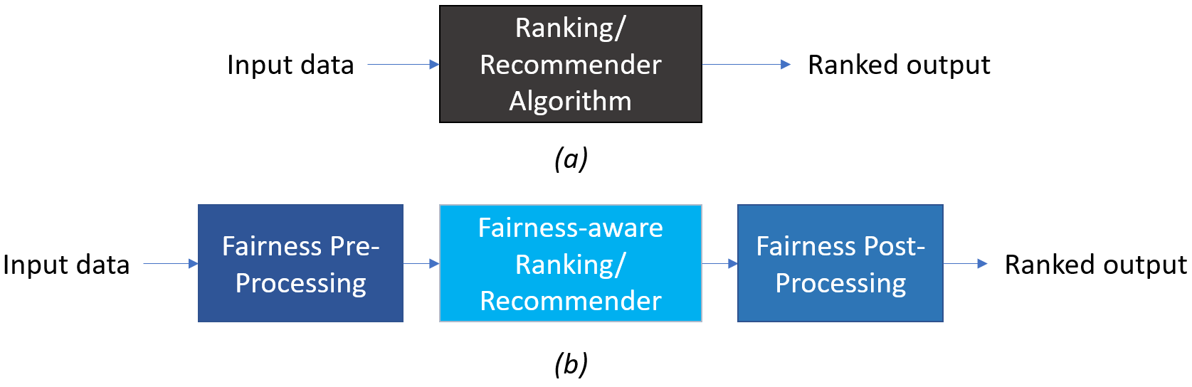
Figure 3: The general distinction of the methods for ensuring fair ranked outputs.

• Pre-processing methods aim at transforming the data to remove any underlying bias or discrimination. Typically, such methods are application agnostic, and consider bias in the training data (which they try to mitigate). Bias in the data may be produced due to the data collection process (for example, based on decisions about the pieces of data we collect or not, or what assumptions we make for the missing values), or even when using data in a different way than intended during collection.

• In-processing methods aim at modifying existing or introducing new algorithms that result in fair rankings and recommendations, e.g., by removing bias and discrimination during the model training process. Typically, such methods targets at learning a model with no bias, while considering fairness during the training of a model, for example, by incorporating changes into the objective function of an algorithm by a fairness term or imposing fairness constraints, without offering any guarantees about fairness on the ranked outputs.

• Post-processing methods modify the output of the algorithm. Typically, such methods can only treat the ranking or recommendation algorithm as a black box without any ability to modify it, and to improve fairness they re-rank the data items of the output. Naturally, in post-processing methods, fairness comes at the cost of accuracy, since by definition the methods transform the optimal output. On the other hand, a clear advantage of the post-processing methods is that they offer ranked outputs that are easy to understand, when comparing their outputs with the outputs before any application of a post-processing fairness method.

Next, we will use this taxonomy to organize and present the related works that we describe in the following sections.

5 Pre-processing Methods

Bias in the underlying data on which systems are trained can take two forms. Bias in the rows of the data exists when there are not enough representative individuals from minority groups. For example, according to a Reuters article amazon-jobs-2018 , Amazon’s experimental automated system to review job applicants’ resumes showed a significant gender bias towards male candidates over females that was due to historical discrimination in the training data.

Bias in the columns is when features are biased (correlated) with sensitive attributes. For example, zip code tends to predict race due to a history of segregation amazon-race-2016 . Direct discrimination occurs when protected attributes are used explicitly in making decisions (i.e., disparate treatment). More pervasive nowadays is indirect discrimination, in which protected attributes are not used but reliance on variables correlated with them leads to significantly different outcomes for different groups, also known as disparate impact.

To address bias and avoid discrimination, several methods have been proposed for pre-processing data. Many of these methods are studied in the context of classification, while a few have been proposed in the context of recommender systems.

5.1 Suppression

To tackle bias in the data, a naïve approach used in practice is to simply omit the protected attribute (say, race or gender) when training the classifier DBLP:journals/kais/KamiranC11 .

Simply excluding a protected variable is insufficient to avoid discriminatory predictions, as any included variables that are correlated with the protected variables still contain information about the protected characteristic, and the classifier still learns the discrimination reflected in the training data. For example, answers to personality tests identify people with disabilities wsj-2014 . Word embeddings trained on Google News articles exhibit female/male gender stereotypes DBLP:conf/nips/BolukbasiCZSK16 . To tackle such dependencies, one can further find the attributes that correlate most with the sensitive attribute and remove these as well.

5.2 Class Relabeling

This approach, also known as massaging DBLP:journals/kais/KamiranC11 , changes the labels of some objects in the dataset in order to remove the discrimination from the input data. A good selection of which labels to change is essential. The idea is to consider a subset of data from the minority group as promotion candidates, and change their class label. Similarly, a subset of the majority group is chosen as demotion candidates. To select the best candidates for relabeling, a ranker is used that ranks the objects based on their probability of having positive labels. For example, a Naïve Bayesian classifier can be used for both ranking and learning 4909197 ; DBLP:journals/kais/KamiranC11 . Then, the top-k minority, for promotion, objects and the bottom-k majority, for demotion, objects are chosen. The number $k$ of pairs needed to be modified to make a dataset $D$ discrimination-free can be calculated as follows.

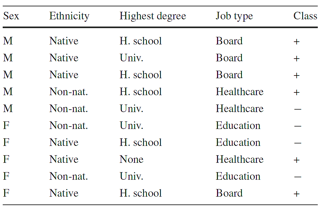
Figure 4: Job application example DBLP:journals/kais/KamiranC11 .

Let us assume as before two groups, namely, the protected group $G^{+}$ and the non-protected (or, privileged) group $G^{-}$. If we modify $k$ objects from each group, the resulting discrimination will be:

$$\frac{p^{-}-k}{|G^{-}|}-\frac{p^{+}+k}{|G^{+}|}=disc(D)-k(\frac{1}{|G^{+}|}+\frac{1}{|G^{-}|})=$$

$$disc(D)-(k\frac{|D|}{|G^{-}||G^{+}|})$$ (31)

To reach zero discrimination, the number of modifications needed is:

$$k=\frac{disc(D)\times|G^{-}|\times|G^{+}|}{|D|}$$ (32)

where $p^{+}$ ($p^{-}$) are the number of positive objects that belong to the minority group (majority group). Discrimination $disc(D)$ in $D$ is the probability of being in the positive class between the objects in the minority group versus those in the majority group.

For example, consider the dataset in Figure 4. This dataset contains the Sex, Ethnicity, and Highest Degree for 10 job applicants, the Job Type they applied for, and the outcome of the selection procedure, Class. We want to learn a classifier to predict the class of objects for which the predictions are non-discriminatory toward females. We can rank the objects by their positive class probability given by a a Naïve Bayes classification model. Figure 5 shows an extra column that gives the probability that each applicant belongs to the positive class. In the second step, we arrange the data separately for female applicants with class $-$ in descending order and for male applicants with class $+$ in ascending order with respect to their positive class probability. The ordered promotion and demotion candidates are given in Figure 6. To reach zero discrimination, the number of modifications needed is:

$$k=\frac{disc(D)\times|G^{F}-|\times|G^{M}+|}{|D|}=\frac{0.4\times 5\times 5}{10}=1$$ (33)

We relabel the highest scoring female with a negative label and the lowest scoring male with a positive label. Then, the discrimination becomes zero. The resulting dataset will be used for training a classifier.

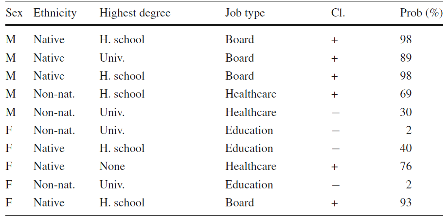
Figure 5: Job applications with positive class probability

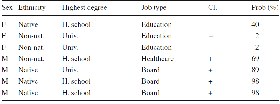
Figure 6: Promotion and demotion candidates

The problem of classification without discrimination w.r.t. a sensitive attribute is a multi-objective optimization problem. Lowering the discrimination will result in lowering the accuracy and vice versa.

5.3 Reweighing

The previous approach is rather intrusive as it changes the labels of the objects. Instead of that, weights can be assigned to the objects to compensate for the bias DBLP:journals/kais/KamiranC11 . The idea is to assign lower weights to objects that have been deprived or favored. Then, the weights can be used directly in any method based on frequency counts.

A frequently used family of analytical methods are grouped under propensity score matching JSSv042i08 . Such methods model the probability of each object or group receiving the treatment and use these predicted probabilities or “propensities” to make up for the confounding of the treatment with the other variables of interest and balance the data.

A simple probability-based reweighing method is the following DBLP:journals/kais/KamiranC11 . Let us consider the sensitive attribute $S$. Then, every object $x$ will be assigned a weight:

$$w(x)=\frac{P_{exp}(S=x(S)\wedge class=x(class))}{P_{obs}(S=x(S)\wedge class=x(class))}$$ (34)

i.e., the weight of an object will be the expected probability to see an instance with its sensitive attribute value and class given independence, divided by its observed probability.

For example, consider the dataset in Figure 4. If the dataset is unbiased, then the sensitive attribute $S$ (i.e., sex in our example) and the class are statistically independent. Then, the expected probability for females to be promoted would be: $P_{exp}(sex=F\wedge class=+)=0.5*0.6=0.3$. In reality, however, the observed probability based on the dataset is $P(sex=F\wedge class=+)=0.2$. Hence, one can use a re-weighting factor $w(x)=0.3/0.2=1.5$ to balance the bias in the dataset.

Entropy balancing aims at covariate balance in data for binary classification hainmueller2012 . It relies on a maximum entropy reweighting scheme that calibrates individual weights so that the reweighed groups satisfy a set of balance constraints that are imposed on the sample moments of the covariate distributions. The balance constraints ensure that the reweighed groups match exactly on the specified moments adjusting in this way inequalities in representation. The generated weights can be passed to any standard classifier.

Adaptive Sensitive Reweighing uses a convex model to estimate distributions of underlying labels with which to adapt weights Krasanakis2018 . It assumes that there exists an (unobservable) underlying set of class labels corresponding to training samples that, if predicted, would yield unbiased classification with respect to a fairness objective. It searches for sample weights that make weighted training on the original dataset also train towards those labels, without explicitly observing them.

More specifically, consider a binary probabilistic classifier, which produces probability estimates $\hat{P}(Y=y_{i})=1-\hat{P}(Y\neq y_{i})$. For training samples $i$ with features $x_{i}$ and class labels $y_{i}$, there exists an underlying (i.e. unobservable) class labels $\tilde{y_{i}}$ that yield estimated labels $\hat{y_{i}}$ which conform to designated fairness and accuracy trade-offs. The training goal is to minimize both weighted error on observed labels as well as the distance between weighted observed labels and unweighed underlying labels:

$$min\sum_{i}{w_{i}\hat{P}(\hat{y_{i}}\neq y_{i})}$$ (35)

$$min\sum_{i}({w_{i}\hat{P}(\hat{y_{i}}\neq y_{i})-\hat{P}(\hat{y_{i}}\neq\tilde{y_{i}})})^{2}$$ (36)

To simultaneously adjust training weights alongside classifier training, a classifier-agnostic iterative approach is proposed: first, a classifier is fully trained based on uniform weights, and then, the method appropriately readjusts those weights. This process is repeated until convergence.

5.4 Data Transformation

A common theme is the importance of balancing discrimination control against utility of the processed data. This can be formulated as an optimization problem for producing preprocessing transformations that trade off discrimination control, data utility, and individual distortion DBLP:conf/nips/CalmonWVRV17 . Assuming $S$ is the one or more protected (sensitive) variables, $X$ denotes other non-protected variables, and $Y$ is an outcome random variable. The goal is to determine a randomized mapping $P_{\hat{X,Y}|X,Y,S}$ that transforms both the training data and the test data. The mapping should satisfy three properties.

$-$ Discrimination Control. The first objective is to limit the dependence of the transformed outcome $\hat{Y}$ on the protected variables $S$, which requires the conditional distribution $P_{\hat{Y}|S}$ to be close to a target distribution $P_{Y_{T}}$ for all values of $S$.

$-$ Distortion Control. The mapping $P_{\hat{X,Y}|X,Y,S}$ should satisfy distortion constraints to reduce or avoid certain large changes (e.g. a very low credit score being mapped to a very high credit score).

$-$ Utility Preservation. The distribution of ($\hat{X},\hat{Y}$) should be statistically close to the distribution of $(X,Y)$. This is to ensure that a model learned from the transformed data (when averaged over the protected variables $S$) is not too different from one learned from the original data. For example, a bank’ s existing policy for approving loans does not change much when learnt over the transformed data.

5.5 Database Repair

Handling bias in the data can be considered a database repair problem. One approach is to remove information about the protected variables from the set of covariates to be used in predictive models FFM+15 ; DBLP:journals/corr/LumJ16 . A test for disparate impact based on how well the protected class can be predicted from the other attributes and a data repair algorithm for numerical attributes have been proposed FFM+15 . The algorithm “strongly preserves rank”, which means it changes the data in such a way that predicting the class is still possible. A chain of conditional models can be used for both protecting and adjusting variables of arbitrary type DBLP:journals/corr/LumJ16 . This framework allows for an arbitrary number of variables to be adjusted and for each of these variables and the protected variables to be continuous or discrete.

Another data repair approach is based on measuring the discriminatory causal influence of the protected attribute on the outcome of an algorithm. This approach removes discrimination by repairing the training data in order to remove the effect of any discriminatory causal relationship between the protected attribute and classifier predictions DBLP:conf/sigmod/SalimiRHS19 . This work introduced the notion of interventional fairness, which ensures that the protected attribute does not affect the output of the algorithm in any configuration of the system obtained by fixing other variables at some arbitrary values. The system repairs the input data by inserting or removing tuples, changing the empirical probability distribution to remove the influence of the protected attribute on the outcome through any causal pathway that includes inadmissible attributes, i.e. attributes that should not influence the protected attribute.

5.6 Data Augmentation

A different approach is augment the training data with additional data DBLP:conf/wsdm/RastegarpanahGC19 . This framework starts from an existing matrix factorization recommender system that has already been trained with some input (ratings) data, and adds new users who provide ratings of existing items. The new users’ ratings, called antidote data, are chosen so as to improve a socially relevant property of the recommendations that are provided to the original users. The proposed framework includes measures of both individual and group unfairness.

5.7 Summary of Pre-processing Methods

Table 2 summarizes pre-processing approaches to fairness based on whether they focus on bias in rows or columns, the level of fairness (individual or group) and the algorithm that will use the pre-processed data.

Many of the pre-processing methods are studied in the context of classification/ranking. Suppression is a simple, brute-force approach that does not depend on the algorithm. On the downside, the algorithm may still learn the discrimination from correlated attributes. Trying to remove these attributes as well can seriously hurt the value of the dataset.

The class relabeling approach works with different rankers (e.g., a Naive Bayes classifier, or nearest neighbor classifier). However, its objective is to lower the discrimination, which will result in lowering the accuracy and vice versa. Finding the right balance is challenging. Moreover, it is intrusive as it changes the dataset.

The reweighing methods are parameter-free as they do not rely on a ranker. Hence, they can work with any ranking algorithm as long as they leverage frequencies. Adaptive Sensitive Reweighing has an additional classification overhead since it simultaneously adjusts training weights alongside classifier training through an iterative approach which is repeated until convergence.

Data transformation methods work with different classifiers but they can be applied only on numerical datasets and they modify the data.

The aforementioned approaches modify the training data, explicitly (e.g., by suppressing attributes or changing class labels) or implicitly, e.g., by adding weights. Data augmentation leaves the training data as is and just augment it with additional data. One data augmentation method has been proposed in the context of recommender system, and in particular for matrix factorization. This approach has studied both individual and group fairness DBLP:conf/wsdm/RastegarpanahGC19 . In general, group fairness is easier to track and handle.

There is an abundance of machine learning algorithms used in practice for search and recommendations (and in general) dictating a clear need for a future systematic study of the relationship between dataset features, algorithms, and pre-processing performance.

Table 2: Pre-processing Methods.

	bias in rows	bias in columns	fairness	algorithm
Suppression DBLP:journals/kais/KamiranC11			group	any
Class Relabeling 4909197 ; DBLP:journals/kais/KamiranC11			group	ranker
Reweighing hainmueller2012 ; DBLP:journals/kais/KamiranC11 ; Krasanakis2018			group/ individual	ranker
Data transformation DBLP:conf/nips/CalmonWVRV17			group/ individual	ranker
Data repair FFM+15 ; DBLP:journals/corr/LumJ16 ; DBLP:conf/sigmod/SalimiRHS19			group	ranker
Data augmentation DBLP:conf/wsdm/RastegarpanahGC19			group/ individual	matrix factorization

6 In-processing Methods

In-processing methods for achieving fairness in rankings and recommendations focus on modifying existing or introducing new models or algorithms. In this section, we survey in a unified way these methods, by distinguishing between learning approaches and approaches using preference functions.

6.1 Learning Approaches

For both rankings and recommenders, learning approaches typically use machine learning to construct ranking models, most often using a set of labeled training data as input. In general, the ranking model ranks unseen lists in a way similar to the ranking of the training data. The overall goal is to learn a model that minimizes a loss function that captures the distance between the learned and the input ranking.

Various approaches exist, varying on the form of training data and the type of loss function learning-book . In the point-wise approach (e.g., pointlearn1 ), the training data are (item, relevance-score) pairs for each query. In this case, learning can be seen as a regression problem where given an item and a query, the goal is to predict the score of the item. In the pair-wise approach, the training data are pairs of items where the first item is more relevant than the second item for a given query pairlearn1 ; pairlearn2 . In this case, learning can be seen as a binary classification problem where given two items, the classifier decides whether the first item is better than the second one. Finally, in the list-wise approach (e.g., listnet ), the input consists of a query and a list of items ordered by their relevance to the query. Note that the loss function takes many different forms depending on the approach. For example, in the pair-wise approach, loss may be computed as the average number of inversions in a ranked output.

In the following, we present a number of approaches towards making the ranking models fair. Note that the proposed approaches can be adopted to work for different types of input data and loss functions.

6.1.1 Adding Regularization Terms

A general in-processing approach to achieving fairness is by adding regularization terms to the loss function of the learning model. These regularization terms express measures of unfairness that the model must minimize in addition to the minimization of the original loss function. Depending on the form of the training data, the loss function and the measure of fairness, different instantiations of this general approach are possible.

The DELTR approach ZDC20 extends the ListNet listnet learning to rank framework. ListNet is a list-wise framework where the training set consists of a query $q$ and a list of items ordered by their relevance to $q$. ListNet learns a ranking function $f$ that minimizes a loss function $L_{LN}$ that measures the extent to which the ordering $\hat{r}$ of items induced by $f$ for a query differs from the ordering $r$ that the items appear in the training set for this query. The loss function $L_{DELTR}$ of DELTR is:

$$L_{DELTR}(r(q),\hat{r}(q))=L_{LN}(r(q),\hat{r}(q))+\\ \lambda\,Unfairness(\hat{r}(q))$$ (37)

$L_{DELTR}$ extends the original loss function $L_{LN}$ of ListNet with a term that imposes a fairness constraint. Parameter $\lambda$ controls the trade-off between ranking utility (i.e., distance from input ranking $r$ captured by the original loss function) and fairness.

Exposure is used as a measure of unfairness in the produced output. Specifically:

$$Unfairness(r(q))=max\{0,Exposure(G^{+}|r(q)-\\ Exposure(G^{-}|r(q))^{2}$$ (38)

Using the squared hinge loss makes the loss function differentiable. Also, the model prefers rankings in which the exposure of the protected group is not less than the exposure of the non-protected group but not vice versa.

A regularization approach is also taken for recommender systems in DBLP:conf/fat/KamishimaAAS18 . Let $U$ and $I$ denote random variables for the users and items respectively and $R$ denote a random variable for the recommendation output. Let also $S$ be the sensitive attribute, that is, information to be ignored in the recommendation process, like the gender of a user or the popularity of an item. The goal in this case, is to achieve recommendation, or statistical, independence. This means to include no information about the sensitive feature that influences the outcome, as well as recommendations should satisfy a recommendation independence constraint.

The core of this regularization approach is included in Equation 39 that adopts a regularizer imposing a constraint of independence, while training the recommendation model.

$$\sum_{D}loss(r_{i},r(x_{i},y_{i},s_{i}))-\eta\cdot ind(R,S)+\lambda\cdot reg(\theta)$$ (39)

where $\eta$ is the independence parameter that controls the balance between independence and accuracy and $ind$ is the independence term, i.e., the regularizer to constrain independence; the larger value indicates that recommendations and sensitive values are more independent. Loss is the empirical loss, while $\lambda$ is the regularization parameter and $\theta$ is the L2 regularizer. Several alternatives can be used for the independence term, like, for example, the mutual information with histogram models or normal distributions, or by exploiting distance measures as in the case of distribution matching using the Bhattacharyya distance.

6.1.2 Learning via Variational Autoencoders

Variational Autoencoders (VAE) are proposed as the state-of-the-art for the collaborative filtering task in recommenders. With a multinomial likelihood generative model and a controlled regularization parameter, it is possible to estimate normal distribution parameters in the middle layer of an MLP, that enriches the rating data representation and outperforms previous neural network based approaches DBLP:conf/www/LiangKHJ18 . The situation requires drawing samples from the inferred distributions in order to propagate values to the decoder, but it is not a trivial task to take gradients when having a sampling step. The re-parametrization trick DBLP:journals/corr/KingmaW13 is to re-parameterize the sampled values by incorporating a normal distributed noise, so the gradient can back-propagate through the sampled variable during the training.

Instead of using only the re-parametrization trick during the training phase, the noise variable can be incorporated in the test phase of VAE as well DBLP:conf/medes/BorgesS19 , in order to enhance fairness in the ranking order of recommendations (using as definition of fairness, Equation 10). The motivation here is that different noise distributions directly affect the rankings, depending on how frequently the latent values vary around the mean inside the interval defined by the variance. Specifically, it is experimentally shown that the noisy effect of the Gaussian and uniform distributions vary the output scores when having the same data as input, while unfairness is reduced despite of a small decrease in the quality of the ranking. The higher the variance of the new component, the greater the effect in the predicted scores, and consequently in the ranking order.

6.1.3 Learning Fair Representations

The main idea in this approach is to learn a fair representation of the input data and use it for the task at hand. Previous work in fair classification used this idea to achieve fairness by introducing an intermediate level $Z$ between the input space $X$ that represents individuals and the output space $Y$ that represents classification outcomes ZWS+13 . $Z$ should be a fair representation of $X$ that best encodes $X$ and obfuscates any information about membership in the protected group. Specifically, $Z$ is modeled as a multinomial random variable of size $k$ where each of the $k$ values represents a prototype (cluster) in the space of $X$.

The goal is to learn $Z$ such that to minimize a loss function $L$:

$$L=\lambda_{x}L_{x}+\lambda_{z}L_{z}+\lambda_{y}L_{y}$$ (40)

where the first term, $L_{x}$, refers to the quality of the encoding, i.e., expresses the requirement that the distance from points in $X$ to their representation in $Z$ should be small, the second term, $L_{z}$, refers to fairness, and the last term, $L_{y}$, refers to accuracy, i.e., the prediction based on the representation should be accurate. Parameters $\lambda_{x}$, $\lambda_{y}$ and $\lambda_{z}$ are hyper-parameters that control the trade-off among these three objectives.

One can enforce different forms of fairness by appropriately defining the $L_{z}$ objective. Statistical parity is used in ZWS+13 captured by the following objective:

$$Pr(z=k|x\in G^{+})=Pr(z=k|x\in G^{-}),\,\forall\,k$$ (41)

that is, the probability that a random element that belongs to the protected group of $X$ maps to a particular prototype of $Z$ is equal to the probability that a random element that belongs to the non-protected group of $X$ maps to the same prototype.

The fair representation approach has also been used for fair ranking instead of classification. This was achieved by modifying the last objective $L_{y}$ in Equation 40 to represent accuracy in the case of ranking as opposed to accuracy in classification YS17 . The modified objective asks that the distance between the ground truth ranking and the estimated ranking is small.

6.2 Linear Preference Functions

In some applications, items are ranked based on a score that is a weighted linear combination of the values of their attributes. Specifically, let $i$ be an item with $d$ scoring attributes, $i[1]\dots i[d]$. A linear ranking function $f$ uses a weight vector $w$ = $(w_{1},\dots w_{d})$, to compute a utility (goodness) score for each item $i$, $f(i)=\sum_{j=1}^{d}w_{j}i[j]$.

In this case, fairness is formulated as the following problem. Given function $f$ with weight vector $w$ = $(w_{1},\dots w_{d})$, find a function $f^{*}$ with weight vector $w^{*}$ = $(w^{*}_{1},\dots w^{*}_{d})$, such that, $f^{*}$ produces a fair ranking and its weights are as close to the weights of the original $f$ as possible, i.e., $cosine(w,w^{*})$ is minimized AJS+19 .

6.3 Constraint Optimization for Rank Aggregation

For fairness-preserving rank aggregation, DBLP:journals/pvldb/KuhlmanR20 presents a solution that balances aggregation accuracy with fairness, using a pairwise rank representation. In this case, a ranking is represented as a set of pairwise comparisons between data items. Then, for two rankings, the number of pairs with items that do not have the same order in the two rankings expresses their Kendall Tau distance kendal1938 . Overall, given a set of rankings, the ranking with the minimum average Kendall Tau distance to the rankings in the set is known as the Kemeny optimal rank aggregation.

Consider the case where we have data items from two different groups, $G^{+}$ and $G^{-}$. The pairs in their Cartesian product can be divided into three subsets: pairs containing items from $G^{+}$, pairs containing items from $G^{-}$, and pairs containing one item from $G^{+}$ and one item from $G^{-}$. Then, $Rpar_{G^{+}}(\rho)$ computes the probability, for a ranking $\rho$, that an item from group $G^{+}$ is ranked above an item from group $G^{-}$:

$$Rpar_{G^{+}}(\rho)=P(x_{i}<_{\rho}x_{j}|x_{i}\in{G^{+}},x_{j}\in{G^{-}})$$ (42)

Following from this, the pairwise formulation of statistical parity for two groups is defined as: Given a ranking $\rho$, consisting of data items that belong to mutually exclusive groups $G^{+}$, $G^{-}$, $\rho$ satisfies pairwise statistical parity if the following condition is met:

$$Rpar_{G^{+}}(\rho)=Rpar_{G^{-}}(\rho)$$ (43)

A linear integer programming solution with parity constraint is offered for aggregating many rankings, while producing a fair consensus. For achieving better efficiency, a branch-and-bound fairness-aware ranking algorithm is designed that integrates a rank parity-preserving heuristic.

In Section 8, we summarize the in-processing methods, along with the post-processing ones, highlighting the advantages of each category.

7 Post-processing Methods

Post-processing approaches are agnostic to the ranking or the recommendation algorithm. Typically, they take as input a ranking $r$ and a specification of the required form of fairness and produce a new ranking $\hat{r}$ that satisfies the fairness requirements and respects the initial ranking, to the extent possible.

7.1 Fairness as a Generative Process

Let us consider a simple case of group parity, where we ask that a specific proportion $p$, $0\leq p\leq 1$, of the items at the top $k$ positions in the ranking belong to the protected group.

Given $p$ and a ranking $r$, the generative process introduced in YS17 creates a ranking $\hat{r}$ by: (a) initializing $\hat{r}$ to the empty list, and (b) incrementally adding items to $\hat{r}$. Specifically, for each position $j$ in $r$, a Bernoulli trial is performed with $p$. If the trial succeeds, we select the best available, i.e., most highly ranked in $r$, item from the protected group. Otherwise, we select the best available item from the non-protected group. An example is shown in Figure 2(c). The ranking $r_{l}$ in the left is the original ranking based on the utility score of the items. The middle ranking $r_{m}$ corresponds to the extreme case of $p=1$ where all members of the protected group are placed in the top positions, while the ranking $t_{r}$ on the right corresponds to $p=0.5$.

The produced ranking $\hat{r}$ satisfies the in-group monotonicity constraints. This means that, within each group, the items are ordered with decreasing qualifications. It is also shown that under some assumptions the ranking also maximizes the utility expressed as the average score of the items in the top-$k$ positions ZBC+17 .

A statistical test for this generative model is proposed in ZBC+17 . Specifically, given that at a specific position we have seen a specific number of items from each group, an one-tailed Binomial test is used to compare the null hypotheses that the ranking was generated using the model with parameter $p*$ = $p$, or with $p*$ $<$ $p$, which would mean that the protected group is represented less than desired.

7.2 Fair Ranking as a Constraint Optimization Problem

Another post-processing approach formulates the problem of producing a fair ranking $\hat{r}$ as an optimization problem. Let $F$ be a fairness measure for rankings and let $U$ be a measure of the utility of a ranking for a particular task, for example, let $U(r|q)$ be the relevance of ranking $r$ for a given query $q$. There are two general ways of formulating an optimization problem involving fairness $F(r)$ and utility $U(r|q)$, namely:

• (maxFcoU) maximizing fairness subject to a constraint in utility,

• (maxUcoF) maximizing utility subject to a constraint in fairness.

In the maxFcoU formulation, the underlying idea is to produce a ranking that is as fair as possible while remaining relevant to $q$ (e.g., BGW18 ). For example, we ask for the most fair ranking $\hat{r}$ among all rankings such that $\hat{r}$ also satisfies a utility constraint, e.g., the loss in utility with regards to the original ranking $r$ remains below a given threshold $\theta$:

$\hat{r}=argmax_{\hat{r}}F(\hat{r})$
    s. t., $distance(U(r|q),U(\hat{r}|q))\leq\theta$.

Alternatively, in the maxUcoF formulation, we look for the ranking that has the the maximum possible utility among all rankings whose fairness is sufficient (e.g., BGW18 , SJ18 ). For example, the approach proposed in SJ18 produces a ranking $r$ such that:

$r=argmax_{r}U(r|Q)$     s.t. $r$ is fair.

We characterize such maxUcoF approaches as post-processing, since they assume that the utility of each item is known, or can be estimated. Thus, implicitly there is an original, non-fair ranking in which the items are ordered solely by their utility. Then, given these individual utilities, a new ranking is produced that also satisfies a fairness constraint.

In general, the complexity of both the maxFcoU and maxUcoF optimization problems depends on the type of the utility and fairness functions, and the form of the constraints. In some cases, the optimization problems can be solved using linear integer programming (ILP), e.g., BGW18 , or, in some special cases using a dynamic programming algorithm e.g., CSV18 .

Constraints can be also used for producing fair recommendation packages of items for groups of users DBLP:conf/www/SerbosQMPT17 . The intuition of the method is to greedily construct a package $P$, by adding in rounds to $P$ the item that satisfies the largest number of non-satisfied users. Specifically, given that $sat_{G}(P)$ denotes the users in $G$ that are satisfied by $P$, at each round, the goal is to maximize:

$$f_{G}(P,i)=|sat_{G}(P\cup{i})\backslash sat_{G}(P)|.$$ (44)

When considering fairness proportionality (Equation 28), $sat_{G}(i)$ contains the users for which item $i$ belongs in their top-$\delta$% most preferable items. For envy-freeness fairness (Equation 27), $sat_{G}(i)$ contains the users that are envy-free for the item $i$. That is, $P$ is fair for a user $u$ (m-proportional, or m-envy-free), if there are at least $m$ items $i$ in $P$, such that, $u\in sat_{G}(i)$.

This method is generalized to include constraints that restrict the set of candidate packages that can be recommended to a group of users. Two types of constraints are discussed, namely category and distance constraints. In simple words, with category constraints, when selecting an item from a specific category, we remove the items of this category from the candidate set. With distance constraints, we consider as candidate items only the items that when added to the existing solution satisfy the specific input distance constraints.

7.3 Fairness via Calibration Methods

Calibration methods suggest to re-rank a list of items as a post-processing step. Equation 19 (in Section 3.2) quantifies the degree of calibration for recommender’s outputs based on specific metrics DBLP:conf/recsys/Steck18 .

To determine the optimal set $I^{*}$ of $N$ recommended items – movies in the suggested scenario – the maximum marginal relevance function DBLP:journals/sigir/CarbinellG17 is used:

$$I^{*}=argmax_{I,|I|=N}(1-\lambda)\cdot s(I)-\lambda\cdot C_{KL}(p,q(I))$$ (45)

where $\lambda\in[0,1]$ determines the trade-off between the prediction scores $s(i)$ of the movies $i\in I$, with $s(I)=\sum_{i\in I}s(i)$, and the calibration metric (Equation 19). Namely, the trade-off between accuracy and calibration is controlled by $\lambda$. Greedily, the method starts with an empty set, and iteratively adds one movie at a time, namely the movie that maximizes Equation 45.

In a similar way, for group recommendations, the best suggestions $I$ for a group $G$ should maximize the social welfare $SW(G,I)$ (Equation 24) and fairness $F(G,I)$ (Equation 25 and 26), using the scheme DBLP:conf/recsys/LinZZGLM17 :

$$\lambda\cdot SW(G,I)+(1-\lambda)\cdot F(G,I).$$ (46)

A greedy solution is to select an item that, when added to the current recommendation list, achieves the highest fairness $F(G,I)$. More time-efficient alternatives are offered via integer programming techniques.

When considering the notion of Pareto optimality for group recommendations, a simple heuristic can be used to compile and approximately identify the list of the top-$N$ recommendations for a group DBLP:conf/sac/Sacharidis19 : Specifically, given $N^{\prime}$, where $N^{\prime}>N$ is the largest number of items the system can recommend for an individual user, the method proceeds as follows: (a) it requests the top-$N^{\prime}$ recommendations for each user in the group, (b) it takes their union, and (c) it identifies the $N$-level Pareto optimal items among the items in the union.

7.4 Fairness in Multiple Outputs

When providing rankings or recommendations, users typically pay more attention to the first positions, and attention wears off for items in lower positions in the ranking. In a situation where the greatest estimated probabilities are quite close or equal to each other, the algorithm needs to arrange them in a proper order and necessarily present high scores in high positions. This promotes an unfair result that can be mitigated in the long term, by changing the position of items in sequential rounds of rankings or recommendations.

In the case of rankings, one approach BGW18 is to require that ranked items receive attention that is proportional to their utility in a sequence of rankings (Equation 9). This way, the unfair position one item appears in a single ranking can be compensated in the next rankings when it changes position, and the whole session contemplates long-term fairness. However, the act of reducing unfairness implies reduction in the ranking quality, due to the perturbation of the utility-based rankings. The trade-off between ranking quality and fairness is formulated as a constrained optimization problem BGW18 targeting at minimizing unfairness subject to constraints on quality (i.e., lower-bound the minimum acceptable quality).

Specifically, for a sequence $\rho^{1}\dots\rho^{m}$ of rankings where the items are ordered by the utility score, inducing zero quality loss, the aim is at reordering them into $\rho^{1*}\dots\rho^{m*}$, to minimize the distance between the attention ($A$) and utility ($U$) distributions with constraints on the NDCG-quality loss in each ranking. Formally:

$$min\sum_{i}|A_{i}-U_{i}|,$$ (47)

subject to $\text{NDCG-quality@k}(\rho^{j},\rho^{j*})\geq\theta,j=1,\ldots,m$,
where $A_{i}$ and $U_{i}$ denote the cumulative attention and utility scores that the item $i$ gained across all rankings.

Consider a different scenario, where a group of users, interacts with a recommender multiple times DBLP:conf/sac/StratigiNPS20 . When following traditional methods for group recommendations, like the average aggregation method and the least misery one, the degree of satisfaction for each user in the group (e.g., Equation 29), can not be good enough for all users in the group, leading to cases in which almost none of the reported items are of interest to some users in the group. That is, the recommender system is unfair to these users, and unfairness continues throughout a number of recommendations rounds. To overcome the drawbacks of the average and the least misery aggregation methods, and capitalize on their advantages, an aggregation method, called sequential hybrid aggregation method, offers a weighted combination of them DBLP:conf/sac/StratigiNPS20 . Specifically:

$$score(G,d_{z},j)=(1-\alpha_{j})*avgScore(G,d_{z},j)+\\ \alpha_{j}*leastScore(G,d_{z},j).$$ (48)

For a group $G$, $avgScore(G,d_{z},j)$ returns the score of the item $d_{z}$ as it is computed by the average aggregation method during round $j$, and $leastScore(G,d_{z},j)$ returns the least satisfied user’s score of $d_{z}$ at round $j$. To self-regulate the value of $\alpha$ between 0 and 1, so as to more effectively describe the consensus of the group, $\alpha$ is set dynamically in each iteration by subtracting the minimum satisfaction score of the group members in the previous iteration, from the maximum score:

$$\alpha_{j}=max_{u\in G}sat(u,Gr_{j-1})-\\ min_{u\in G}sat(u,Gr_{j-1}),$$ (49)

where $sat(u,Gr_{j-1})$ defines the satisfaction of user $u$ for the group recommendations $Gr_{j-1}$ at round $j-1$.

The dynamic calculations of $\alpha$ counteracts the individual drawbacks of the average and least misery method. Intuitively, if the group members are equally satisfied at the last round, then $\alpha$ takes low values, and the aggregation will closely follow that of average, where everyone is treated as an equal. On the other hand, if one group member is extremely unsatisfied in a specific round, then $\alpha$ takes a high value and promotes that member’s preferences on the next round.

Next, we summarize both the in-processing and post-processing methods, and provide their advantages.

8 Summary of In- and Post-processing Methods

In this section, we summarize the in-processing and post-processing approaches for achieving fairness. Overall, there exist methods that have been proposed in the context of rankings, recommender systems, as well as for the rank aggreagation problem. Table 3 organizes the methods based on (a) the level of fairness, namely, individual or group, (b) the side of fairness, namely, consumer or producer, and (c) the output multiplicity, namely, if a method focuses on a single or multiple outputs.

In general, all existing learning and linear preference functions in-processing approaches target group and producer fairness. Most approaches consider a single output with the recent exception of DBLP:conf/medes/BorgesS19 using VAEs that considers multiple outputs. Typically, the approaches in this category extend the objective function that they use by including a fairness, or unfairness, term. The target is to find the best balance between the accuracy objective and fairness objective of the optimization problem that a particular approach applies.

Regarding the post-processing approaches, we observe that there exist works focusing on all different options of fairness definitions. As in the pre-processing case, post-processing methods treat the algorithms for producing rankings and recommendations as black boxes, without changing their inner workings. This means that any post-processing approach receives as input a ranked output, and re-ranks the data items in this output to improve fairness, respecting the initial ranked output, to the extent possible.

Typically, in-processing approaches manage to offer better trade-offs between fairness and accuracy, compared to the post-processing methods, since they naturally identify this balance via the objective function they use. However, at the same time, they cannot offer any guarantees about fairness in the output rankings and recommendations, since fairness is considered only during the training phase. When considering post-processing approaches, it is important to note that they can lead to unpredictable losses in accuracy, since they treat the algorithms for producing rankings and recommendations as black boxes. This is especially true for pre-processing methods as well. On the positive side, post-processing methods offer outputs that are easy to understand, when comparing their outputs with the outputs before any application of a post-processing fairness method, and realize that they offer a fairer output.

Recently, ZWS+13 combines both pre-processing and in-processing strategies by jointly learning a fair representation of the data and the classifier parameters. This approach has two main limitations: (a) it leads to a non-convex optimization problem and does not guarantee optimality, and (b) the accuracy of the classifier depends on the dimension of the fair representation, which needs to be chosen rather arbitrarily.

Table 3: In- and Post-processing Methods.

	Level of fairness		Side of fairness		Output multiplicity
	Individual	Group	Consumer	Producer	Single	Multiple
In-processing methods
Adding regularization terms		ZDC20 ; DBLP:conf/fat/KamishimaAAS18		ZDC20 ; DBLP:conf/fat/KamishimaAAS18	ZDC20 ; DBLP:conf/fat/KamishimaAAS18
Learning fair representations		ZWS+13		ZWS+13	ZWS+13
Learning with VAEs		DBLP:conf/medes/BorgesS19		DBLP:conf/medes/BorgesS19		DBLP:conf/medes/BorgesS19
Linear preference functions		AJS+19		AJS+19	AJS+19
Constraint optimization for rank aggregation		DBLP:journals/pvldb/KuhlmanR20	DBLP:journals/pvldb/KuhlmanR20		DBLP:journals/pvldb/KuhlmanR20
Post-processing methods
Fairness as a generative process		YS17 ; ZBC+17		YS17 ; ZBC+17	YS17 ; ZBC+17
Fairness as a constraint optimization problem	DBLP:conf/www/SerbosQMPT17 ; BGW18	SJ18 ; CSV18	DBLP:conf/www/SerbosQMPT17	SJ18 ; BGW18 ; CSV18	DBLP:conf/www/SerbosQMPT17 ; SJ18 ; CSV18	BGW18
Fairness with calibration methods	DBLP:conf/sac/Sacharidis19 ; DBLP:conf/recsys/LinZZGLM17	DBLP:conf/recsys/Steck18	DBLP:conf/sac/Sacharidis19 ; DBLP:conf/recsys/LinZZGLM17	DBLP:conf/recsys/Steck18	DBLP:conf/sac/Sacharidis19 ; DBLP:conf/recsys/Steck18 ; DBLP:conf/recsys/LinZZGLM17
Fairness in multiple rounds	DBLP:conf/sac/StratigiNPS20 ; BGW18		DBLP:conf/sac/StratigiNPS20	BGW18		DBLP:conf/sac/StratigiNPS20 ; BGW18

9 Verifying Fairness

In the previous sections, we studied methods for achieving fairness. Both pre-processing and post-processing methods treat the recommendation or ranking algorithm as a black box and try to address fairness in the input or the output of the algorithm, respectively. In particular, post-processing methods assume that we already know that we have an algorithm that creates discrimination in its output and try to mitigate that. The question that naturally arises is how we can verify whether a program is fair in the first place.

Program fairness verification aims at analyzing a given decision-making program and constructing a proof of its fairness or unfairness — just as a traditional static program verifier would prove correctness of a program with respect to, for example, lack of divisions by zero. However, there are several challenges: (a) what class of decision-making programs the program model will capture, (b) what the input to the program is, (c) how to describe what it means for the program to be fair, and (d) how to fully automate the verification process.

One simple approach is to take a decision-making program $P$ and a dataset as input DBLP:conf/sigsoft/GalhotraBM17 . Using a concrete dataset simplifies the verification problem but it also raises questions of whether the dataset is representative for the population for which we are trying to prove fairness. An alternative approach would be to use a population model $M$ as input, which can be a probabilistic model that defines a joint probability distribution on the inputs of $P$ DBLP:journals/corr/AlbarghouthiDDN16 . Then, we need to define when and why a program is fair or unfair. If we want to prove group fairness — for example, that the algorithm is just as likely to hire a minority applicant ($m$) as it is for other, non-minority applicants we could define a post-condition like the following DBLP:journals/corr/AlbarghouthiDDN16 :

$\frac{Pr[P(v)=true|v_{s}=m]}{Pr[P(v)=true|v_{s}\neq m]}>1-\epsilon$

The verifier then will prove or disprove that $P$ is fair for the given population.

In general, proving group fairness is easier: the verification process reduces to computing the probability of a number of events with respect to the program and the population model. However, proving individual fairness requires more complex reasoning involving multiple runs of the program, a notoriously hard problem. Moreover, in the case of a negative result, the verifier should provide the users with a proof of unfairness. Depending on the fairness definition, producing a human readable proof might be challenging as the argument might involve multiple and potentially infinite inputs. For example, for group fairness, it might be challenging to explain why the program outputs true on $40\%$ of the minority inputs and on $70\%$ of the majority inputs. Overall, program fairness verification is a difficult, and less investigated, topic.

A different approach is to make fairness a first-class citizen in programming. In fairness-aware programming DBLP:conf/fat/AlbarghouthiV19 , developers can state fairness expectations natively in their code, and have a run-time system monitor decision-making and report violations of fairness. This approach is analogous to the notion of assertions in modern programming languages. For instance, the developer might assert that $x>0$, indicating that they expect the value of $x$ to be positive at a certain point in the code. The difficulty, however, is that fairness definitions are typically probabilistic, and therefore detecting their violation cannot be done through a single execution as in traditional assertions. Instead, we have to monitor the decisions made by the procedure, and then, using statistical tools, infer that a fairness property does not hold with reasonably high confidence.

For example, consider a movie recommendation system, where user data has been used to train a recommender that, given a user profile, recommends a single movie DBLP:conf/fat/AlbarghouthiV19 . Suppose that the recommender was constructed with the goal of ensuring that male users are not isolated from movies with a strong female lead. Then, the developer may add the following specification to their recommender code:

$@spec(pr(femaleLead(r)|s=male)>0.2)$

The above specification ensures that for male users, the procedure recommends a movie with a female lead at least $20\%$ of the time.

To determine that a procedure $f$ satisfies a fairness specification $\phi$, we need to maintain statistics over the inputs and outputs of the procedure $f$ as it is being applied. Specifically, we compile the specification $\phi$ into run-time monitoring code that executes every time $f$ is applied, storing aggregate results of every probability event appearing in $\phi$. In the earlier example with movie recommendation, the monitoring code would maintain the number of times the procedure returned true for a movie with a female lead. Again, a big challenge is checking individual fairness. In this case, the run-time system has to remember all decisions made explicitly, so as to compare new decisions with past ones.

10 Open Challenges

In this paper, we have just begun to realize the need for fairness in particular fields, namely in rankings and recommender systems. Next, we highlight a few critical open issues and challenges for future work, which aim to support advanced services for making accountable complex rankings and recommender systems.

A codification of definitions.

As described in Sections 2 and 3, there is not a universal definition for expressing fairness in rankings and recommenders. Instead, the list of potential definitions is very long.

Specifically, just for fairness alone, there exist a plethora of different definitions. Some of them are not even compatible, in the sense that there is no method that can satisfy all of them simultaneously, except in highly constrained special cases KMR17 . Furthermore, there is also a need to make explicit the correspondence between these definitions and the interpretation of bias or diversity, that each of them materializes. The limitations of each definition, the compatibility among them, the incurred trade-offs, the domain of applicability, assumptions and parameters are not well understood yet.

Moreover, it is interesting to see how the general public views fairness in decision making. By testing people’s perception of different fairness definitions, we can understand definitions of fairness that are appropriate for particular contexts DBLP:conf/www/Grgic-HlacaRGW18 ,DBLP:conf/uss/PlaneRMT17 . One such attempt investigates which definitions people perceive to be the fairest in the context of loan decisions DBLP:conf/aies/SaxenaHDRPL19 , and whether fairness perceptions change with the addition of sensitive information (i.e., race of the loan applicants).

Lack of data.

A major challenge is that the available data is often limited DBLP:conf/icde/AsudehJJ19 . This way, any analysis is done with data that has been acquired independently, through a process on which the data scientist has limited control. Collecting more data for analysis is challenging, and will help to discover more types of biases on it. In the long run, one could envision benchmarks for measuring the societal impact of an algorithm along the lines of the TPC benchmark for database performance.

A unified approach for the data pipeline.

One limitation of the current work is that fairness has been studied for specific tasks in isolation, with most current work in fairness focusing on the classification task with the goal of non-discrimination. However, there is a need to consider fairness along the whole data pipeline DBLP:conf/ssdbm/StoyanovichHAMS17 . This includes pre-processing steps, such as data selection, acquisition, cleaning, filtering and integration. Pre-pro- cessing for removing bias, can be viewed as the action of repairing, e.g., by replacing, modifying, or deleting data that cause bias. This pipeline also includes post-processing steps, such as data representation, data visualization and user interfaces. For example, how results are presented can introduce bias, and this is why we need to understand the implications for fairness.

Lack of evaluation tools.

Besides coming up with the correct way of defining fairness in rankings and recommenders, there is also a need for tools for investigating bias, and evaluating the quality of a dataset, an algorithm, or a system. There are some first attempts, such as IBM’s AI Fairness 360 and Tensor Flow’s Fairness Indicators. However, both of them focus mainly on statistical group measures of fairness in classification. Concepts, like context and provenance, are important and can be directly considered in designing such tools.

In this direction, we also need efficient ways for measuring fairness and monitoring its evolution over time. Previous research in stream processing and incrementally maintaining statistics may be relevant here.

Perhaps the most pending question is how to quantify the long-term impact of enforcing methods that target at ensuring fairness. Would they work in favor of the social good, or would they backfire in ways that we cannot predict?

Lack of real applications of fairness.

While a lot of work is done in a research setting, we still do not see many actual applications and their results. There are many challenges in making algorithms and systems fairer in the real-world. A company, for example, needs to consider its business metrics (e.g., click-through rate, purchases) and make sure that these are not affected. For example, how to design algorithms that take into account all these different objectives is challenging.

An example of a real application of fairness is found in LinkedIn DBLP:conf/kdd/GeyikAK19 , where they developed a fair framework and they applied it to LinkedIn Talent Search. Online A/B tests showed considerable improvement in the fairness metrics without a significant impact on the business metrics, which paved the way for deployment to LinkedIn users worldwide.

A multi-level architecture of value systems and algorithms.

A problem intrinsic to the definition of all fairness definitions in rankings and recommenders is the fact that they attempt to quantify philosophical, legal, often elusive, and even controversial notions of justice and social good. Complexity is aggregated when notions that reflect value systems and beliefs interact with the mechanisms for implementing them. In the very least, there should be a clear distinction between what constitutes a belief and what is the mechanism, or measure, for codifying this belief. From a technical point of view, we should then be able to focus on assessing whether a proposed measure is an appropriate codification of a given belief as opposed to assessing the belief itself.

This calls for developing different levels of abstractions and mappings between them. This is somehow reminiscent of how data independence is supported in database management systems by the three-level architecture with the physical, conceptual, and external level and the mappings between these levels DBLP:books/daglib/0011128 . At the lower level, we could have beliefs and value systems and at the higher level fairness definitions. Intermediate levels could be used to support transformations for getting from the lower to the higher level.

Relating algorithmic fairness with other notions of fairness in systems.

The focus of this survey is on fairness in decision-making processes, and in particular on rankings and recommendation systems used in this context. However, there are several other cases where a system needs to make decisions, and where fairness is also important. In particular, there are several problems more familiar to the data management community, such as resource allocation and scheduling, where fairness has been studied. We present here representative examples.

For instance, an approach is presented in DBLP:conf/sigmod/KunjirFMB17 for cache allocation where fairness is based on Pareto efficiency and sharing incentives. A multiple resource allocation approach is introduced in DBLP:conf/nsdi/GhodsiZHKSS10 that generalizes max-min fairness to multiple resource types, where max-min fairness in this context refers to maximizing the minimum allocation received by a user in the system. Another notion of fairness, termed proportionate progress, is proposed in DBLP:journals/algorithmica/BaruahCPV96 for the periodic scheduling problem where weighted resources are allocated to tasks for specific time units in each interval. In proportionate progress fairness, each task is scheduled resources according to its importance (i.e., its weight). Finally, for scheduling, in DBLP:conf/edbt/GuptaMWD09 , fairness means that the workload scheduler performs in a way that no query starves for resources.

Another notion of fairness, for a different problem, namely the chairman selection problem, is proposed in DBLP:journals/dm/Tijdeman80 . In the chairman selection problem, a set of states want to form a union and select a chairman for each year. Fairness in this context refers to guaranteeing a small discrepancy for the number of chairmen representing each state, so that all states are satisfied.

Clearly, fairness concerns have emerged in various contexts through the years. Providing a unified view of all these different notions of fairness and the computational methods used to enforce them is an open problem and an opportunity. How to embed models and algorithms for fairness into any system that involves any type of decision making is also open. Of course, new models and algorithms may be needed in different contexts, where the principles of fairness may be different. What works well for a recommendation problem may not work well for a query optimizer or resource sharing in cloud computing. However, this unified view will potentially provide new insights and opportunities for cross-fertilization.

Fairness in other domains.

In this paper, we have focused on ranking and recommendation algorithms. Many more algorithms are being revisited under the lens of fairness. Two such examples are clustering and ranking in networks. For instance, fair clustering adopts a parity definition of fairness and asks that each group must have approximately equal representation in every cluster fairlets . For the link analysis problem in networks, fair algorithms are introduced in DBLP:conf/www/Tsioutsiouliklis21 that use a parity-based definition of fairness and apply constraints on the proportion of Pagerank allocated to the members of each group of nodes in the network.

Algorithmic fairness is a fast changing field. It is an open challenge to provide fairness measures and definitions for all kinds of algorithms and use them in evaluating such algorithms, in analogy of, say response time, for measuring performance pit20 .

Recently, the concept of fairness has also been studied in different domains and for covering different needs. We discuss two such domains, labor market and social matching. For instance, previous research examines labor market cases under fairness concerns and shows the relevance of such concerns on economic outcomes especially when considering employment contracts over time AnnualReviewEconomics09 . Recently, in the same domain, the work in HuC18 pinpoints the persistence of racial inequalities and designs solutions with respect to a dynamic reputational model of the labor market, highlighting the results from groups divergent accesses to resources. Other recent work examines the fairness of online job marketplaces in terms of ranking job applicants sihem . Instead of partitioning the individuals in predefined groups, the authors seek to find a partitioning of the individuals based on their protected attributes that exhibits the highest unfairness.

For the problem of professional social matching, conventional mechanisms, such as optimizing for similarity and triadic closure, are studied in DBLP:journals/cacm/0002HK20 and shown to involve risks of strengthening the homophily bias and echo chambering. For the problem of team assembly, the work in DBLP:conf/webi/MachadoS19 designs fairness-aware solutions when multidisciplinary teams need to be formed and allocated to work on different projects with requirements on members’ skills.

The application of models and mechanisms of algorithmic fairness in a variety of domains that involve social and economic activities, such as in labor market, social matching and team formation, opens a lot of opportunities for fruitful interdisciplinary work.

11 Conclusions

Ranking and recommender systems have several applications, such as hiring, lending, and college admissions, where the notion of fairness is very important since decision making is involved. We have only begun to understand the nature, representation and variety of the several definitions of fairness, and the appropriate methods for ensuring it.

In this article, we follow a systematic and structured approach to explain the various sides of and approaches to fairness. First, we lay the ground by presenting general fairness definitions. Then, we zoom in on models and definitions for rankings, recommendations and the problem of rank aggregation. We organize them in a taxonomy and highlight their differences and commonalities. This analysis naturally leads to a number of open questions, like: (a) How do fairness definitions fare? (b) Which definition is suitable for which context? (c) How do people perceive fairness in different contexts? (d) What does it mean to be fair after all? Is there a unified way to be able to judge whether an outcome or an algorithm is fair?

We move on to describing solutions for fair rankings and recommendations. We organize the approaches to tackle unfairness or ensure a fairer outcome into pre-, in- and post-processing approaches. Within each category, we further classify them along several dimensions. It is still very early to say which one works best for which context. There is no evaluation that puts them all under the same lens and there are generally not conclusive results as to which fare better. It may be the case that a combination of methods should be applied, e.g., combining pre-processing and in-processing steps. This is also an open question as different efforts have adapted a single angle in the problem.

While the focus of this survey is on fairness in rankings and recommendation systems, we discuss several other cases where a system needs to make decisions and fairness is also important, and how we can verify whether a program is fair. Finally, we discuss open research challenges pertaining to fairness in the broader context of data management and on designing, building, managing, and evaluating fair data systems and applications.

References

- (1) A.Chouldechova: Fair prediction with disparate impact: A study of bias in recidivism prediction instruments. Big Data 5(2), 153–163 (2017)
- (2) et al, J.A.: Machine bias. ProPublica (2016). URL https://www.propublica.org/article/machine-bias-risk-assessments-in-criminal-sentencing
- (3) Albarghouthi, A., D’Antoni, L., Drews, S., Nori, A.V.: Fairness as a program property. CoRR abs/1610.06067 (2016). URL http://arxiv.org/abs/1610.06067
- (4) Albarghouthi, A., Vinitsky, S.: Fairness-aware programming. In: Proceedings of the Conference on Fairness, Accountability, and Transparency, FAT* 2019, pp. 211–219. ACM (2019)
- (5) Amer-Yahia, S., Roy, S.B., Chawla, A., Das, G., Yu, C.: Group recommendation: Semantics and efficiency. Proc. VLDB Endow. 2(1), 754–765 (2009)
- (6) Asudeh, A., Jagadish, H.V.: Fairly evaluating and scoring items in a data set. Proc. VLDB Endow. 13(12), 3445–3448 (2020)
- (7) Asudeh, A., Jagadish, H.V., Stoyanovich, J., Das, G.: Designing fair ranking schemes. In: Proceedings of the 2019 International Conference on Management of Data, SIGMOD Conference 2019, pp. 1259–1276. ACM (2019)
- (8) Asudeh, A., Jin, Z., Jagadish, H.V.: Assessing and remedying coverage for a given dataset. In: 35th IEEE International Conference on Data Engineering, ICDE 2019, pp. 554–565. IEEE (2019)
- (9) Baeza-Yates, R.: Bias on the web. Commun. ACM 61(6), 54–61 (2018)
- (10) Baruah, S.K., Cohen, N.K., Plaxton, C.G., Varvel, D.A.: Proportionate progress: A notion of fairness in resource allocation. Algorithmica 15(6), 600–625 (1996)
- (11) Beutel, A., Chen, J., Doshi, T., Qian, H., Wei, L., Wu, Y., Heldt, L., Zhao, Z., Hong, L., Chi, E.H., Goodrow, C.: Fairness in recommendation ranking through pairwise comparisons. In: Proceedings of the 25th ACM SIGKDD International Conference on Knowledge Discovery & Data Mining, KDD 2019, pp. 2212–2220. ACM (2019)
- (12) Biega, A.J., Gummadi, K.P., Weikum, G.: Equity of attention: Amortizing individual fairness in rankings. In: The 41st International ACM SIGIR Conference on Research & Development in Information Retrieval, SIGIR 2018, pp. 405–414. ACM (2018)
- (13) Bolukbasi, T., Chang, K., Zou, J.Y., Saligrama, V., Kalai, A.T.: Man is to computer programmer as woman is to homemaker? debiasing word embeddings. In: Advances in Neural Information Processing Systems 29: Annual Conference on Neural Information Processing Systems 2016, pp. 4349–4357 (2016)
- (14) Borges, R., Stefanidis, K.: Enhancing long term fairness in recommendations with variational autoencoders. In: 11th International Conference on Management of Digital EcoSystems, MEDES 2019, pp. 95–102. ACM (2019)
- (15) Burges, C.J.C., Shaked, T., Renshaw, E., Lazier, A., Deeds, M., Hamilton, N., Hullender, G.N.: Learning to rank using gradient descent. In: Machine Learning, Proceedings of the Twenty-Second International Conference (ICML 2005), ACM International Conference Proceeding Series, vol. 119, pp. 89–96. ACM (2005)
- (16) Calders, T., Verwer, S.: Three naive bayes approaches for discrimination-free classification. Data Min. Knowl. Discov. 21(2), 277–292 (2010)
- (17) Cao, Z., Qin, T., Liu, T., Tsai, M., Li, H.: Learning to rank: from pairwise approach to listwise approach. In: Machine Learning, Proceedings of the Twenty-Fourth International Conference (ICML 2007), ACM International Conference Proceeding Series, vol. 227, pp. 129–136. ACM (2007)
- (18) Carbinell, J., Goldstein, J.: The use of mmr, diversity-based reranking for reordering documents and producing summaries. SIGIR Forum 51(2), 209–210 (2017)
- (19) Celis, L.E., Straszak, D., Vishnoi, N.K.: Ranking with fairness constraints. In: 45th International Colloquium on Automata, Languages, and Programming, ICALP 2018, LIPIcs, vol. 107, pp. 28:1–28:15. Schloss Dagstuhl - Leibniz-Zentrum für Informatik (2018)
- (20) Chierichetti, F., Kumar, R., Lattanzi, S., Vassilvitskii, S.: Fair clustering through fairlets. In: Advances in Neural Information Processing Systems 30: Annual Conference on Neural Information Processing Systems 2017, December 4-9, 2017, Long Beach, CA, USA, pp. 5029–5037 (2017)
- (21) Chouldechova, A., Roth, A.: A snapshot of the frontiers of fairness in machine learning. Commun. ACM 63(5), 82–89 (2020). DOI 10.1145/3376898. URL https://doi.org/10.1145/3376898
- (22) Crammer, K., Singer, Y.: Pranking with ranking. In: Advances in Neural Information Processing Systems 14 [Neural Information Processing Systems: Natural and Synthetic, NIPS 2001], pp. 641–647. MIT Press (2001)
- (23) Dastin, J.: Rpt-insight-amazon scraps secret ai recruiting tool that showed bias against women. Reuters (2018)
- (24) Dwork, C., Hardt, M., Pitassi, T., Reingold, O., Zemel, R.S.: Fairness through awareness. In: Innovations in Theoretical Computer Science 2012, pp. 214–226. ACM (2012)
- (25) Ekstrand, M.D., Burke, R., Diaz, F.: Fairness and discrimination in retrieval and recommendation. In: Proceedings of the 42nd International ACM SIGIR Conference on Research and Development in Information Retrieval, SIGIR 2019, pp. 1403–1404. ACM (2019)
- (26) Elbassuoni, S., Amer-Yahia, S., Ghizzawi, A.: Fairness of scoring in online job marketplaces. Trans. Data Sci. 1(4), 29:1–29:30 (2020)
- (27) Fehr, E., Goette, L., Zehnder, C.: A behavioral account of the labor market: The role of fairness concerns. Annual Review of Economics 1, 355–384 (2009)
- (28) Feldman, M., Friedler, S.A., Moeller, J., Scheidegger, C., Venkatasubramanian, S.: Certifying and removing disparate impact. In: Proceedings of the 21th ACM SIGKDD International Conference on Knowledge Discovery and Data Mining, pp. 259–268. ACM (2015)
- (29) Ferraro, A., Serra, X., Bauer, C.: Break the loop: Gender imbalance in music recommenders. In: F. Scholer, P. Thomas, D. Elsweiler, H. Joho, N. Kando, C. Smith (eds.) CHIIR ’21: ACM SIGIR Conference on Human Information Interaction and Retrieval, Canberra, ACT, Australia, March 14-19, 2021, pp. 249–254. ACM (2021). DOI 10.1145/3406522.3446033. URL https://doi.org/10.1145/3406522.3446033
- (30) Freund, Y., Iyer, R.D., Schapire, R.E., Singer, Y.: An efficient boosting algorithm for combining preferences. In: Proceedings of the Fifteenth International Conference on Machine Learning (ICML 1998), pp. 170–178. Morgan Kaufmann (1998)
- (31) Friedler, S.A., Scheidegger, C., Venkatasubramanian, S.: On the (im)possibility of fairness. CoRR abs/1609.07236 (2016). URL http://arxiv.org/abs/1609.07236
- (32) Friedler, S.A., Scheidegger, C., Venkatasubramanian, S.: The (im)possibility of fairness: different value systems require different mechanisms for fair decision making. Commun. ACM 64(4), 136–143 (2021)
- (33) Friedler, S.A., Scheidegger, C., Venkatasubramanian, S., Choudhary, S., Hamilton, E.P., Roth, D.: A comparative study of fairness-enhancing interventions in machine learning. In: Proceedings of the Conference on Fairness, Accountability, and Transparency, FAT* 2019, pp. 329–338. ACM (2019)
- (34) Galhotra, S., Brun, Y., Meliou, A.: Fairness testing: testing software for discrimination. In: Proceedings of the 2017 11th Joint Meeting on Foundations of Software Engineering, ESEC/FSE 2017, pp. 498–510. ACM (2017)
- (35) Geyik, S.C., Ambler, S., Kenthapadi, K.: Fairness-aware ranking in search & recommendation systems with application to linkedin talent search. In: Proceedings of the 25th ACM SIGKDD International Conference on Knowledge Discovery & Data Mining, KDD 2019, pp. 2221–2231. ACM (2019)
- (36) Ghodsi, A., Zaharia, M., Hindman, B., Konwinski, A., Shenker, S., Stoica, I.: Dominant resource fairness: Fair allocation of multiple resource types. In: Proceedings of the 8th USENIX Symposium on Networked Systems Design and Implementation, NSDI 2011. USENIX Association (2011)
- (37) Grgic-Hlaca, N., Redmiles, E.M., Gummadi, K.P., Weller, A.: Human perceptions of fairness in algorithmic decision making: A case study of criminal risk prediction. In: Proceedings of the 2018 World Wide Web Conference on World Wide Web, WWW 2018, pp. 903–912. ACM (2018)
- (38) Gupta, C., Mehta, A., Wang, S., Dayal, U.: Fair, effective, efficient and differentiated scheduling in an enterprise data warehouse. In: EDBT 2009, 12th International Conference on Extending Database Technology, ACM International Conference Proceeding Series, vol. 360, pp. 696–707. ACM (2009)
- (39) Hainmueller, J.: Entropy balancing for causal effects: A multivariate reweighting method to produce balanced samples in observational studies. Political Analysis 20(1), 25–46 (2012)
- (40) Hardt, M., Price, E., Srebro, N.: Equality of opportunity in supervised learning. In: NIPS, pp. 3315–3323 (2016)
- (41) Ho, D., Imai, K., King, G., Stuart, E.: Matchit: Nonparametric preprocessing for parametric causal inference. Journal of Statistical Software, Articles 42(8), 1–28 (2011)
- (42) Hu, L., Chen, Y.: A short-term intervention for long-term fairness in the labor market. In: Proceedings of the 2018 World Wide Web Conference on World Wide Web, WWW 2018, Lyon, France, April 23-27, 2018, pp. 1389–1398. ACM (2018)
- (43) Imana, B., Korolova, A., Heidemann, J.: Auditing for discrimination in algorithms delivering job ads. In: Proceedings of the Web Conference 2021 (WWW ’21) (2021). DOI 10.1145/3442381.3450077. URL https://doi.org/10.1145/3442381.3450077
- (44) Ingold, D., Soper, S.: Amazon doesn’t consider the race of its customers. should it? Bloomberg (2016)
- (45) Ingold, D., Soper, S.: Amazon doesn’t consider the race of its customers. should it? (2016)
- (46) Jameson, A., Smyth, B.: Recommendation to groups. In: The Adaptive Web, Methods and Strategies of Web Personalization, Lecture Notes in Computer Science, vol. 4321, pp. 596–627. Springer (2007)
- (47) Kamiran, F., Calders, T.: Classifying without discriminating. In: 2009 2nd International Conference on Computer, Control and Communication, pp. 1–6 (2009)
- (48) Kamiran, F., Calders, T.: Data preprocessing techniques for classification without discrimination. Knowl. Inf. Syst. 33(1), 1–33 (2011)
- (49) Kamishima, T., Akaho, S., Asoh, H., Sakuma, J.: Recommendation independence. In: Conference on Fairness, Accountability and Transparency, FAT 2018, Proceedings of Machine Learning Research, vol. 81, pp. 187–201. PMLR (2018)
- (50) Kay, M., Matuszek, C., Munson, S.A.: Unequal representation and gender stereotypes in image search results for occupations. In: Proceedings of the 33rd Annual ACM Conference on Human Factors in Computing Systems, CHI 2015, pp. 3819–3828. ACM (2015)
- (51) Kendall, M.G.: A new measure of rank correlation. Biometrika 30(1), 81–93 (1938)
- (52) Kingma, D.P., Welling, M.: Auto-encoding variational bayes. In: 2nd International Conference on Learning Representations, ICLR 2014 (2014)
- (53) Kleinberg, J.M., Mullainathan, S., Raghavan, M.: Inherent trade-offs in the fair determination of risk scores. In: 8th Innovations in Theoretical Computer Science Conference, ITCS 2017, LIPIcs, vol. 67, pp. 43:1–43:23. Schloss Dagstuhl - Leibniz-Zentrum für Informatik (2017)
- (54) Krasanakis, E., Spyromitros-Xioufis, E., Papadopoulos, S., Kompatsiaris, I.: Adaptive sensitive reweighting to mitigate bias in fairness-aware classification. pp. 853–862 (2018)
- (55) Kuhlman, C., Rundensteiner, E.A.: Rank aggregation algorithms for fair consensus. Proc. VLDB Endow. 13(11), 2706–2719 (2020)
- (56) Kunjir, M., Fain, B., Munagala, K., Babu, S.: ROBUS: fair cache allocation for data-parallel workloads. In: Proceedings of the 2017 ACM International Conference on Management of Data, SIGMOD Conference 2017, pp. 219–234. ACM (2017)
- (57) Kusner, M.J., Loftus, J.R., Russell, C., Silva, R.: Counterfactual fairness. In: Advances in Neural Information Processing Systems 30: Annual Conference on Neural Information Processing Systems 2017, pp. 4066–4076 (2017)
- (58) Liang, D., Krishnan, R.G., Hoffman, M.D., Jebara, T.: Variational autoencoders for collaborative filtering. In: Proceedings of the 2018 World Wide Web Conference on World Wide Web, WWW 2018, pp. 689–698. ACM (2018)
- (59) Lin, X., Zhang, M., Zhang, Y., Gu, Z., Liu, Y., Ma, S.: Fairness-aware group recommendation with pareto-efficiency. In: Proceedings of the Eleventh ACM Conference on Recommender Systems, RecSys 2017, pp. 107–115. ACM (2017)
- (60) Liu, T.: Learning to Rank for Information Retrieval. Springer (2011). DOI 10.1007/978-3-642-14267-3
- (61) Lum, K., Johndrow, J.E.: A statistical framework for fair predictive algorithms. CoRR abs/1610.08077 (2016). URL http://arxiv.org/abs/1610.08077
- (62) Machado, L., Stefanidis, K.: Fair team recommendations for multidisciplinary projects. In: 2019 IEEE/WIC/ACM International Conference on Web Intelligence, WI 2019, Thessaloniki, Greece, October 14-17, 2019, pp. 293–297. ACM (2019)
- (63) Martin, N.: How social media has changed how we consume news. Forbes (2018). URL https://www.forbes.com/sites/nicolemartin1/2018/11/30/how-social-media-has-changed-how-we-consume-news/#18ae4c093c3c
- (64) Ntoutsi, E., Stefanidis, K., Nørvåg, K., Kriegel, H.: Fast group recommendations by applying user clustering. In: Conceptual Modeling - 31st International Conference ER 2012 Proceedings, Lecture Notes in Computer Science, vol. 7532, pp. 126–140. Springer (2012)
- (65) Olsson, T., Huhtamäki, J., Kärkkäinen, H.: Directions for professional social matching systems. Commun. ACM 63(2), 60–69 (2020)
- (66) Oosterhuis, H., Jagerman, R., de Rijke, M.: Unbiased learning to rank: Counterfactual and online approaches. In: A.E.F. Seghrouchni, G. Sukthankar, T. Liu, M. van Steen (eds.) Companion of The 2020 Web Conference 2020, pp. 299–300. ACM / IW3C2 (2020)
- (67) du Pin Calmon, F., Wei, D., Vinzamuri, B., Ramamurthy, K.N., Varshney, K.R.: Optimized pre-processing for discrimination prevention. In: Advances in Neural Information Processing Systems 30: Annual Conference on Neural Information Processing Systems 2017, pp. 3992–4001 (2017)
- (68) Pitoura, E.: Social-minded measures of data quality: Fairness, diversity, and lack of bias. ACM J. Data Inf. Qual. 12(3), 12:1–12:8 (2020)
- (69) Plane, A.C., Redmiles, E.M., Mazurek, M.L., Tschantz, M.C.: Exploring user perceptions of discrimination in online targeted advertising. In: 26th USENIX Security Symposium, USENIX Security 2017, pp. 935–951. USENIX Association (2017)
- (70) Ramakrishnan, R., Gehrke, J.: Database management systems (3. ed.). McGraw-Hill (2003)
- (71) Rastegarpanah, B., Gummadi, K.P., Crovella, M.: Fighting fire with fire: Using antidote data to improve polarization and fairness of recommender systems. In: Proceedings of the Twelfth ACM International Conference on Web Search and Data Mining, WSDM 2019, pp. 231–239. ACM (2019)
- (72) Roy, S.B., Amer-Yahia, S., Chawla, A., Das, G., Yu, C.: Space efficiency in group recommendation. VLDB J. 19(6), 877–900 (2010)
- (73) Sacharidis, D.: Top-n group recommendations with fairness. In: Proceedings of the 34th ACM/SIGAPP Symposium on Applied Computing, SAC 2019, pp. 1663–1670. ACM (2019)
- (74) Salimi, B., Rodriguez, L., Howe, B., Suciu, D.: Interventional fairness: Causal database repair for algorithmic fairness. In: Proceedings of the 2019 International Conference on Management of Data, SIGMOD Conference 2019, pp. 793–810. ACM (2019)
- (75) Saxena, N.A., Huang, K., DeFilippis, E., Radanovic, G., Parkes, D.C., Liu, Y.: How do fairness definitions fare?: Examining public attitudes towards algorithmic definitions of fairness. In: Proceedings of the 2019 AAAI/ACM Conference on AI, Ethics, and Society, AIES 2019, pp. 99–106. ACM (2019)
- (76) Serbos, D., Qi, S., Mamoulis, N., Pitoura, E., Tsaparas, P.: Fairness in package-to-group recommendations. In: Proceedings of the 26th International Conference on World Wide Web, WWW 2017, pp. 371–379. ACM (2017)
- (77) Singh, A., Joachims, T.: Fairness of exposure in rankings. In: Proceedings of the 24th ACM SIGKDD International Conference on Knowledge Discovery & Data Mining, KDD 2018, pp. 2219–2228. ACM (2018)
- (78) Steck, H.: Calibrated recommendations. In: Proceedings of the 12th ACM Conference on Recommender Systems, RecSys 2018, pp. 154–162. ACM (2018)
- (79) Stoyanovich, J., Howe, B., Abiteboul, S., Miklau, G., Sahuguet, A., Weikum, G.: Fides: Towards a platform for responsible data science. In: Proceedings of the 29th International Conference on Scientific and Statistical Database Management, SSDBM 2017, pp. 26:1–26:6. ACM (2017)
- (80) Stratigi, M., Nummenmaa, J., Pitoura, E., Stefanidis, K.: Fair sequential group recommendations. In: SAC ’20: The 35th ACM/SIGAPP Symposium on Applied Computing, pp. 1443–1452. ACM (2020)
- (81) Sweeney, L.: Discrimination in online ad delivery. Commun. ACM 56(5), 44–54 (2013)
- (82) Tijdeman, R.: The chairman assignment problem. Discret. Math. 32(3), 323–330 (1980)
- (83) Tsioutsiouliklis, S., Pitoura, E., Tsaparas, P., Kleftakis, I., Mamoulis, N.: Fairness-aware pagerank. In: WWW ’21: The Web Conference 2021, Virtual Event / Ljubljana, Slovenia, April 19-23, 2021, pp. 3815–3826. ACM / IW3C2 (2021)
- (84) Verma, S., Rubin, J.: Fairness definitions explained. In: Proceedings of the International Workshop on Software Fairness, FairWare@ICSE 2018, pp. 1–7. ACM (2018)
- (85) Weber, L., Dwoskin, E.: Are workplace personality tests fair? Wall Street Journal (2014)
- (86) Xie, M., Lakshmanan, L.V.S., Wood, P.T.: Composite recommendations: from items to packages. Frontiers Comput. Sci. 6(3), 264–277 (2012)
- (87) Yang, K., Stoyanovich, J.: Measuring fairness in ranked outputs. In: Proceedings of the 29th International Conference on Scientific and Statistical Database Management, SSDBM 2017, pp. 22:1–22:6. ACM (2017)
- (88) Yao, S., Huang, B.: Beyond parity: Fairness objectives for collaborative filtering. In: Advances in Neural Information Processing Systems 30: Annual Conference on Neural Information Processing Systems 2017, pp. 2921–2930 (2017)
- (89) Zehlike, M., Bonchi, F., Castillo, C., Hajian, S., Megahed, M., Baeza-Yates, R.: Fa*ir: A fair top-k ranking algorithm. In: Proceedings of the 2017 ACM on Conference on Information and Knowledge Management, CIKM 2017, pp. 1569–1578. ACM (2017)
- (90) Zehlike, M., Diehn, G.T., Castillo, C.: Reducing disparate exposure in ranking: A learning to rank approach. In: The Web Conf (WWW). ACM (2020)
- (91) Zehlike, M., Yang, K., Stoyanovich, J.: Fairness in ranking: A survey. CoRR abs/2103.14000 (2021)
- (92) Zemel, R.S., Wu, Y., Swersky, K., Pitassi, T., Dwork, C.: Learning fair representations. In: Proceedings of the 30th International Conference on Machine Learning, ICML 2013, JMLR Workshop and Conference Proceedings, vol. 28, pp. 325–333. JMLR.org (2013)