On Uncertainty Quantification in the Parametrization of Newman-type Models of Lithium-ion Batteries

Abstract

We consider the problem of parameterizing Newman-type models of Li-ion batteries focusing on quantifying the inherent uncertainty of this process and its dependence on the discharge rate. In order to rule out genuine experimental error and instead isolate the intrinsic uncertainty of model fitting, we concentrate on an idealized setting where “synthetic” measurements in the form of voltage curves are manufactured using the full, and most accurate, Newman model with parameter values considered “true”, whereas parameterization is performed using simplified versions of the model, namely, the single-particle model and its recently proposed corrected version. By framing the problem in this way, we are able to eliminate aspects which affect uncertainty, but are hard to quantity such as, e.g., experimental errors. The parameterization is performed by formulating an inverse problem which is solved using a state-of-the-art Bayesian approach in which the parameters to be inferred are represented in terms of suitable probability distributions; this allows us to assess the uncertainty of their reconstruction. The key finding is that while at slow discharge rates the voltage curves can be reconstructed quite accurately, this can be achieved with some parameter varying by 300% or more, thus providing evidence for very high uncertainty of the parameter inference process. As the discharge rate increases, the reconstruction uncertainty is reduced but at the same time the fits to the voltage curves becomes less accurate. These observations highlight the ill-posedness of the inverse problem of parameter reconstruction in models of Li-ion battery operation. In practice, using simplified model appears to be a viable and useful strategy provided that the assumptions facilitating the model simplification are truly valid for the battery operating regimes in which the data was collected.

Keywords:

Lithium-ion batteries, Newman model, reduced-order models, inverse modelling, parametrization, uncertainty quantification

1 Introduction

Lithium-ion batteries (LiBs) are already produced in their billions each year and the industry is set to grow significantly over the coming decades as electric vehicles rise in prevalence [1, 2]. Even though the technology is already widespread, improvements in cell lifetime, recyclability, and increased charging rates are required. This development can be accelerated by supplementing practical work with accurate models allowing in-silico testing of novel designs without the need for costly and time-consuming physical prototyping.

The Doyle-Fuller-Newman (DFN) model is the most-commonly used modelling framework for describing the operation of LiBs on the scale of anode-cathode pairs, i.e., on the cell level [3, 4, 5, 6]. Its utility has been demonstrated many times, e.g., in [7, 8, 9, 10], and it has been systematically derived and analyzed in numerous other works, see, e.g., [11, 12, 13, 14, 15]. The model is physics-based, and has enough fidelity to predict the changes in performance that result from alterations in meaningful device parameters, yet it is also coarse enough that it can be solved on feasible timescales using relatively modest computational resources. However, a persistent difficulty lies in developing robust techniques to accurately estimate the large number of scalar material properties and state-dependent constitutive relations that are needed to parameterize it. Depending on which variant of the DFN model is being used, typical numbers of parameters are in the range of 15–30. Experimental methods can used to measure many of the required parameters (within the limits of experimental error) and recent years have seen examples of studies that have been able to obtain complete parameterization for certain cells [16, 17, 18, 19]. Despite this, complete experimental characterization remains difficult, time consuming and requires specialized equipment.

Inverse modelling is an approach that can be used in parallel with experimental characterization to help obtain parameters that cannot be readily measured. The basic idea is to combine measurement data with mathematical models of the processes to infer unknown parameters, typically by minimizing the discrepancy between the measured quantities and the corresponding quantities predicted by the model using methods of numerical optimization. One type of electrochemical data which has been often used for this purpose because it is relatively easy to obtain are discharge voltage curves. The efficacy of the approach in battery modelling has already been demonstrated a number of times, see e.g., [20, 21, 22], but the inverse modelling approach becomes increasingly harder to apply as the number of model parameters increases.

The main difficulty is that inverse problems tend to be ill-posed, in the sense that they usually do not admit exact solutions in the form of parameters such that the corresponding model predictions would match the measurements exactly. On the other hand, inverse problems typically admit many, often infinitely-many, approximate solutions where the model predictions corresponding to the inferred parameters match the measurements only approximately. This ill-posedness has roots in weak dependence of the model predictions on some of its parameters and is compounded by experimental noise and numerical errors unavoidably present in approximations of the model equations and in the solution of the optimization problem. Faced with a multitude of possible approximate solutions, it is important to assign relative uncertainties to each of them. However, this is difficult when the inverse problem is formulated in the classical way by defining the error functional and then minimizing it with respect to unknown parameters using methods of numerical optimization, a procedure which normally yields one set of “optimal” parameters. On the other hand, uncertainty of reconstructed parameters can be conveniently characterized in the framework of Bayesian inference which recently began to attract a lot of attention [23, 24, 25]. The main idea is to frame the inverse problem in probabilistic terms, such that unknown parameters are inferred in terms of their probability distributions. Recent applications of this approach to problems in electrochemistry are described in [26, 27, 28].

The use of more, or higher-fidelity, experimental data can help mitigate the problem described above, but another complimentary approach is to write down simplified models, which contain fewer parameters and to fit those instead. This latter strategy comes with the caveat that one must take care that the simplified model is still complete enough that it accurately captures the important physical/chemical processes within the LiB. Thus, there are subtle trade-offs between the fidelity of models, their parametrizability and their subsequent utility.

The main goal of this paper is to demonstrate, for what we believe to be the first time in the electrochemical literature, that even in simple settings inverse modelling can in fact lead to ambiguous results. This will be done by analyzing the uncertainty of parameterization of relatively simple models introduced below using methods of Bayesian inference and “measurements” obtained with the DFN model. By framing the problem in this way we eliminate experimental measurement errors and ensure all numerical errors are strictly controlled, such that we can focus on the effect of ill-posedness.

To fix attention, we focus on modelling a cathode made from nickel manganese cobalt oxide Li(Ni_0.4Co_0.6)O₂, a material also known as NMC or LNC whose properties were studied in [16, 17]. In fact, the set-up of our problem can be regarded as a highly simplified “in silico” version of these experiments. In the next section we describe the hierarchy of models that will be used in this study, first outlining the DFN model and then describing the Single Particle Model (SP) and its corrected variant (cSP). Next, in Section 3 we describe the Bayesian approach to inverse modelling with uncertainty quantification. Computational results are presented in Section 4 whereas final conclusions and outlook are deferred to Section 5. Some additional technical material is collected in Appendix A.

2 Electrochemical models

In this section we introduce a hierarchy of models describing transport of electrochemically active species in a cell. We will focus on the galvanostatic set-up where the applied external current $I(t)$ is considered as the input and the drop of the voltage across the cell $V(t)$ is the main output. First, we present the classical DFN model also known as the pseudo 2D (P2D) model. Developed by Newman and his co-workers in the mid-’90s and early 2000’s [3, 4, 5], the DFN model is based on transport equations for lithium ions in the electrolyte and for lithium atoms in the active particles of the electrodes (the cathode and the anode) coupled through the Butler-Volmer relations describing the intercalation and de-intercalation of lithium at the interface between active particles and the electrolyte. The DFN model has the form of a parabolic-elliptic system of partial differential equations (PDEs) which after discretization in space leads to a system of differential-algebraic equations (DAEs). This model is thus computationally complex which limits its use in some applications.

The complexity of the DFN model is the motivation behind the development of reduced-order models. One such model is the single-particle (SP) model in which it is assumed that particles throughout the electrode thickness behave in the same way such that the transport in only a single particle needs to be solved for. Systematic derivations of the SP model from the DFN model have been given in [29, 30] and other justifications have been given in [31, 32, 33].

The corrected single-particle (cSP) model is derived using a formal asymptotic method applied to the DFN model [30]. It is based on the disparity between the size of thermal voltage and of the characteristic change in overpotential that occurs during (de)lithiation. It has the advantage that it more accurately reproduces the voltage predicted by the DFN model than the SP model but is slightly more expensive to solve (though still markedly simpler than the full DFN model. The two reduced-order models are related since the asymptotic limit of large changes in the open-circuit voltage (OCV) relative to the thermal voltage recovers a variant of the SP model at leading order because the reaction overpotentials are small.

For simplicity of presentation, we will focus here on the half-cell geometry illustrated schematically in Figure 1 where the coordinate $x$ measures distance across the cell and $r$ is the radial coordinate in the active particles.

Figure 1: A schematic diagram of the half-cell geometry. The anode is made from lithium metal, the separator is located between $x=-L_{s}$ and $x=0$, and the cathode current collector is at $x=L$.

2.1 Doyle-Fuller-Newman (DFN) model

We now briefly state the DFN model.

Macroscopic equations.

The equations governing ionic transport through the electrolyte and those governing electronic transport through the porous binder matrix are

$$\epsilon_{l}\frac{\partial c}{\partial t}+\frac{\partial{N}_{-}}{\partial x}=0,\quad{N}_{-}=-\mathcal{B}D_{\rm{eff}}(c)\frac{\partial c}{\partial x}-(1-t_{0}^{+})\frac{j}{F}\quad\mbox{in}\quad-L_{s}<x<L,$$ (1)

$$\frac{\partial j}{\partial x}=bj_{n},\qquad j=-\mathcal{B}\kappa(c)\left(\frac{\partial\Phi}{\partial x}-\frac{2R_{g}T}{F}\frac{1-t_{0}^{+}}{c}\frac{\partial c}{\partial x}\right)\quad\mbox{in}\quad L_{s}<x<L,$$ (2)

$$\frac{\partial j_{s}}{\partial x}=-bj_{n},\quad j_{s}=-{\sigma_{s}}\frac{\partial\Phi_{s}}{\partial x}\quad\mbox{in}\quad 0<x<L,$$ (3)

$$j_{n}=\left\{\begin{array}[]{ccc}0&\mbox{in}&-L_{s}<x<0,\\ \displaystyle 2Fkc^{1/2}\left(c_{s}\rvert_{r=R}\right)^{1/2}\left(c_{s}^{\rm max}-c_{s}\rvert_{r=R}\right)^{1/2}\sinh\left(\frac{F\eta}{2R_{g}T}\right)&\mbox{in}&0\leq x<L,\end{array}\right.$$ (6)

$$\eta=\Phi_{s}-\Phi-U_{eq}(c_{s}|_{r=R}).$$ (7)

Here $x$ and $t$ denote position through the electrode and time respectively, $L$ and $L_{s}$ are the widths of the separator and electrode respectively, $\epsilon_{l}$ is the volume fraction of active material, $c$ is the molar concentration of lithium ions in the electrolyte, ${N}_{-}$ is the effective flux of negative counterion across the electrolyte, $\mathcal{B}$ is the permeability factor, $D_{\rm{eff}}$ is the ionic diffusivity, $t_{0}^{+}$ is the transference number, $j$ and $j_{s}$ are the ionic and electronic current densities, $F$ is Faraday’s constant, $R_{g}$ is the universal gas constant, $T$ is the absolute temperature, $b$ is the Brunauer-Emmett-Teller (BET) surface area, $\kappa$ is the ionic conductivity, $j_{n}$ is the current density carried by the Butler-Volmer reaction, $\Phi$, $\Phi_{s}$ are the electric potential in the electrolyte and electrode respectively, $\sigma_{s}$ is the conductivity of the electrode and $U_{\rm eq},c_{s}^{\rm max}$ and $R$ are the equilibrium potential, the maximum concentration that can be stored in the electrode material, and the radius of the electrode particles located at the macroscopic coordinate $x$.

Macroscopic boundary conditions.

We impose boundary conditions requiring that: (i) the Li-metal counter-electrode supplies an ionic current density of $\frac{I(t)}{A}$ to the electrolyte on $x=-L_{s}$; (ii) current of density $\frac{I(t)}{A}$ is extracted from the solid phase of the electrode at the current collector $x=L$; and (iii) at $x=0$ no current flows from the solid phase into the separator. In addition, (iv) the potential $\Phi$ in the electrolyte is specified on $x=-L_{s}$ (edge of the separator) and (v) and (vi) there is no counterion flux across the interfaces between the electrolyte and the separator and between the electrolyte and the current collector. In summary, this gives, cf. Figure 1,

$$j|_{x=-L_{s}}=\frac{I}{A},\quad{N}_{-}|_{x=-L_{s}}=0,\quad\Phi|_{x=-L_{s}}=0,\quad{N}_{-}|_{x=L}=0.$$ (8)

$$j_{s}|_{x=0}=0,\quad j_{s}|_{x=L}=\frac{I}{A}.$$ (9)

Microscopic equations and boundary conditions.

Conservation of lithium in a single spherical active material particle of radius $R$ is described by the diffusion equation with suitable boundary conditions

$$\frac{\partial c_{s}}{\partial t}=\frac{1}{r^{2}}\frac{\partial}{\partial r}\left(r^{2}D_{s}(c_{s})\frac{\partial c_{s}}{\partial r}\right)\quad\mbox{in}\quad 0<r<R,$$ (10)

$$c_{s}\,\,\mbox{bounded}\,\,\mbox{on}\,\,r=0,\qquad-D_{s}(c_{s})\frac{\partial c_{s}}{\partial r}\bigg{\rvert}_{r=R}=\frac{j_{n}}{F}\ \ \mbox{in}\ \ 0<x<L.$$ (11)

Initial conditions.

Furthermore, partial differential equations from the system (1)–(11) require initial conditions on concentration in electrolyte $c$ and in electrode $c_{s}$. Initially, we assume that electrode is in a state of equilibrium, i.e., $I(0)=0$, and $j_{n}(x,0)=0$ then gives the uniform electrolyte salt concentration

$$c|_{t=0}=c_{init}\quad\mbox{in}\quad-L_{s}<x<L,$$ (12)

and a uniform lithium concentration in all the electrode particles

$$c_{s}|_{t=0}=c_{s,init}\quad\mbox{in}\quad 0<r<R.$$ (13)

These conditions together imply that $\Phi(x,0)=0$ and $\Phi_{s}(x,0)=U_{\rm eq}(c_{s,init})$.

Geometry.

We assume that all electrode particles are spherical such that the BET surface area $b$ and electrode particle volume fraction $\epsilon_{s}$ are related by the expression

$$\epsilon_{s}=\frac{bR}{3}.$$ (14)

Furthermore, the electrolyte volume fraction $\epsilon_{l}$ is related to $\epsilon_{s}$ by

$$\epsilon_{l}=1-\epsilon_{inert}-\epsilon_{s},$$ (15)

where $\epsilon_{inert}$ is the volume fraction of electrochemically inert material.

The half-cell potential.

Once the model equations have been solved, the half-cell potential $V$ can be evaluated using

$$V(t)=\Phi_{s}|_{x=L}.$$ (16)

C-rate.

It is common to quantify the current being drawn from/supplied to a cell using a measure called the C-rate; this is a dimensionless quantity defined to be the present current supply/draw divided by the current supply/draw that is needed to “fully (dis)charge” the cell in one hour. In the interests of consistency, we shall define our C-rate in the same fashion as was done by Ecker et. al. in [16, 17] who experimentally determined that a current of 0.15625A “fully utilized” their LNC cathode in 1 hour. Our C-rate is then defined as

$$\text{C-rate}=\frac{I}{0.15625}$$ (17)

and can be changed by varying the current $I$.

We note that there is a small discrepancy between the cell capacity implied by Ecker et. al.’s experimental measurement and the theoretical capacity (which is marginally higher). An upshot of this is that later, see e.g., Figure 6, we are able to maintain cell operation for slightly longer than expected.

2.2 Single-particle (SP) model

As the most common approximation to the DFN model (1)–(13), the SP model is obtained by assuming that the cell voltage only depends upon the potential of the insertion material. To determine this quantity we solve only for transport in a single representative insertion particle. All other potential drops are neglected, including that across the electrolyte, across the solid, and across the interfaces (double layers) between the electrolyte and insertion material caused the interfacial resistance. There are different instances when this level of simplification is justified, for example, during low C-rate operation. The SP model is then given by

$$\frac{\partial c_{s}}{\partial t}=\frac{1}{r^{2}}\frac{\partial}{\partial r}\left(r^{2}D_{s}(c_{s})\frac{\partial c_{s}}{\partial r}\right)\quad\mbox{in}\quad 0<r<R,$$ (18)

$$c_{s}\,\,\mbox{bounded}\,\,\mbox{on}\,\,r=0,\qquad c_{s}|_{r=R}=\mathcal{C}(t),\qquad c_{s}|_{t=0}=c_{s,init},$$ (19)

$$\int_{0}^{L}j_{n}(x,t)dx=-\frac{I(t)}{Ab},\,\,\mbox{where}\,\,j_{n}=-FD_{s}(c_{s})\frac{\partial c_{s}}{\partial r}\bigg{\rvert}_{r=R},$$ (20)

where lithium concentration on the surface of the electrode particle is $\mathcal{C}(t)$ and the relation (20) implies that the total reaction output is equal to the net current $I(t)$ thus ensuring the conservation of charge. The voltage $V(t)$ of the half-cell is then estimated using

$$V(t)=U_{\rm eq}\left(\mathcal{C}(t)\right).$$ (21)

A systematic derivation of the SP model from the DFN model based on the asymptotic limit of large electrode and electrolyte conductivities and large electrolyte diffusivity is presented in [29], whereas an extension of this model is introduced in [33]. Parameter and state estimation problems for the SP model were recently considered in [31, 34]. Similar asymptotic techniques for LiB in the context of a porous electrode model have been used in [35].

2.3 Corrected single-particle (cSP) model

The corrected single-particle (cSP) model introduced in [30] is accurate for materials that have an overpotential which varies appreciably with concentration (in practice, these are most common electrode materials, except for lithium-iron-phosphate) and for sufficiently low C-rates. However, it is worth emphasizing that, as demonstrated in [30], the cSP model remains accurate for much larger C-rates than the SP model.

The cSP model consists of the standard SP model (18)–(21) supplemented by the governing equations for the electrolyte concentration and potential given in (1)–(2) which are subject to the boundary and initial condition

$$j|_{x=-L_{s}}=\frac{I(t)}{A},\quad{N}_{-}|_{x=-L_{s}}=0\quad\Phi|_{x=-L_{s}}=0,\quad{N}_{-}|_{x=L}=0,$$ (22)

$$c|_{t=0}=c_{init}.$$ (23)

The model equations for the SP model are decoupled from those for the electrolyte and can hence be solved first. Subsequently, the evolution of the concentration and potential in the electrolyte is found and, at this stage, the Butler-Volmer current density is known from (11b). Finally, we calculate the corrected half-cell voltage by evaluating

$$V(t)=U_{\rm eq}(\mathcal{C}(t))+\frac{\int_{0}^{L}\left[\eta(x,t)+\Phi(x,t)-\int_{0}^{L}\frac{j_{s}(x^{\prime},t)dx^{\prime}}{\sigma_{s}}\right]dx}{L},$$ (24)

where the current density is given by

$$j_{s}(x,t)=\frac{I}{A}-j(x,t)$$ (25)

and overpotential is

$$\eta(x,t)=2\frac{R_{g}T}{F}\operatorname{arcsinh}\left(\frac{j_{n}(x,t)}{2Fk\left[(c_{s}^{\rm max}-\mathcal{C}(t))\mathcal{C}(t)c\right]^{1/2}}\right).$$ (26)

2.4 Test Problems

Our aim is to assess the uncertainty in the calibration of the SP and cSP models by solving suitably defined Bayesian inverse problems where the “measurements” will be generated by solving the DFN model and will serve as psuedo-experimental data. By framing the problem in this way we eliminate various experimental measurement errors and this will allow us to concentrate on sources of calibration uncertainty intrinsic to the models themselves. We focus on modelling a half-cell made from nickel manganese cobalt oxide Li(Ni_0.4Co_0.6)O₂ and shown schematically in Figure 1. A complete data set of the material properties and constitutive relations characterizing this cell for the purposes of solving the DFN model is collected in Table 1. The parameters that we will later take to be unknown for the purposes of inverse modelling are marked with a dagger (^†). Exactly which parameters can be determined by inverse modelling depends upon the model being utilized; many parameters in the DFN model do not appear in the simplified models. This information is summarized in Table 2. In the case of the cSP model we elect to take the vector of unknown parameters to be ${\mathbf{P}}=[\mathcal{B},\sigma_{s},\widehat{D},R,\widehat{D}_{s}]$. Here the quantities $\widehat{D}$ and $\widehat{D}_{s}$ might aptly be referred to as the “characteristic size” of the diffusivity in the electrolyte and LNC respectively. More precisely they are defined as follows

$$D(x) =\widehat{D}\,[0.278x^{3}-1.356x^{2}+1.87x+0.180]x^{-1},$$ (27)

$$D_{s}(x) =\widehat{D}_{s}\,[4.7-4.3\exp(-12(x-0.62)^{2})],$$ (28)

cf. Figures 2(a,c), so that changing the hatted quantities corresponds to maintaining the functional form of the diffusivity but modifies its magnitude by a multiplicative factor. We frame the inverse modelling problem using the hatted quantities (rather than the functions $D(x)$ and $D_{s}(x)$ themselves) because it is markedly simpler to infer a scalar quantity than a function. This being said, the latter task has been accomplished in [21, 36]. In the case of the SP model the situation is more nuanced since the parameters $R$ and $\widehat{D}_{s}$ enter as a product and therefore cannot be independently determined. Thus, for the SP model we will assume that the particle radius is known $R=6.5\mu m$, cf. Table 1, and will infer the diffusivity coefficient $\widehat{D}_{s}$ such that in this case the vector of unknown parameters will be ${\mathbf{P}}=[\widehat{D}_{s}]$.

We will consider the problem of discharging the cell under different rates, namely, 2C, 4C, 8C and 16C. This will allow us to see how the discharging rate affects the uncertainty of parameter estimation. Since time-dependent discharge voltage curves are relatively easy to obtain in experiments, we will use these quantities predicted the DFN model at the different discharging rates as our “measurements”. They will be denoted $\widetilde{V}(t)$ for $0\leq t\leq t_{f}$, where $t_{f}$ is the duration of the simulated experiment which depends on the C-rate. More specifically, for each C-rate the discharge time $t_{f}$ is chosen to achieve the same voltage drop, namely, such that $\widetilde{V}(t_{f})=3.58$ V, see Figures 6(a,c,e,g) further below. This ensures that close to 100% of charge is extracted from the cell and gives $t_{f}=0.529,0.254,0.109,0.037$ hrs for 2C, 4C, 8C and 16C. To summarize, our goal will be to infer “true” values of the parameters ${\mathbf{P}}$ using the SP and cSP models based on “measurements” generated by the more complete DFN model. The specific question we want to address is how the accuracy and uncertainty of this calibration process depends on the model and the C-rate.

   

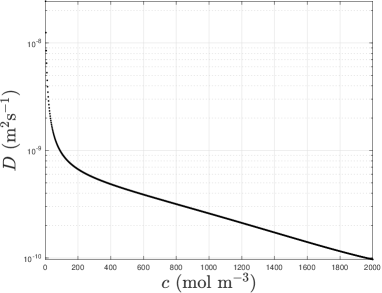
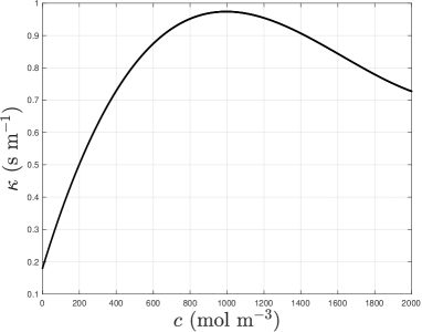
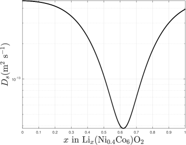
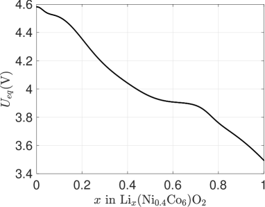
Figure 2: State-dependent material properties: (a) ionic diffusivity, (b) conductivity of the liquid phase, (c) diffusivity in the solid phase and (d) equilibrium potential of Li(Ni_0.4Co_0.6)O₂.

Param./	Description	Value and Units
Function
$L$	Electrode thickness	54 $\mu$m
$R^{\dagger}$	Electrode particle radius	6.5 $\mu$m
$A$	Electrode cross-section area	8.585 $\times 10^{-3}$ m2
$\epsilon_{l}$	Volume fraction of electrolyte in electrode matrix	0.296 (dim’less)
$b$	Particle surface area per unit volume electrode	3.249 $\times 10^{5}$ (m-1)
$k$	Reaction rate constant	5.904$\times 10^{-11}$ (mol-1/2m5/2s-1)
$c_{s}^{max}$	Maximum concentration of Li+ in solid	28176.4 (mol m-3)
$c_{\text{init}}$	Typical concentration of Li in electrolyte	1000 (mol $m^{-3}$)
$t_{0}^{+}$	Transference number	0.26 (dim’less)
$\cal B^{\dagger}$	Permeability factor in electrode matrix	0.153 (dim’less)
$\sigma_{s}^{\dagger}$	Conductivity in solid	68.1(Sm-1)
$U_{\rm eq}$	Equilibrium potential	Figure 2(d) (V)
$I$	Current flow into cell	0.15625 (A)
$\widehat{D}^{\dagger}$	Typical diffusivity in electrolyte	2.549$\times 10^{-10}$ (m2 s-1)
$\widehat{D}_{s}^{\dagger}$	Typical diffusivity in solid	$10^{-13}$ (m2 s-1)
$\widehat{\kappa}$	Typical conductivity in electrolyte	1 ( sm2 )
$T$	Absolute temperature	298.15 (K)
$F$	Faraday’s constant	$96487$(A s mol-1)
$R_{g}$	Universal gas constant	$8.3145$ (J K-1mol-1)

Table 1: Physical constants and material properties characterizing a cathode made from Li(Ni_0.4Co_0.6)O₂. The material properties which are not constant and are functions of state parameters are shown in Figure 2. Quantities denoted with a dagger (^†) are considered unknown and will be inferred via inverse modelling, cf. Table 2.

Parameters	DFN Model	cSP model	SP model
$\cal B$	$\checkmark$	$\checkmark$
$\sigma_{s}$	$\checkmark$	$\checkmark$
$\widehat{D}$	$\checkmark$	$\checkmark$
$R$	$\checkmark$	$\checkmark$	$\checkmark$
$\widehat{D}_{s}$	$\checkmark$	$\checkmark$	$\checkmark$

Table 2: Unknown material properties which can be inferred via inverse modelling using different models (a tick $\checkmark$ indicates that the given parameter appears in the model).

3 Inverse Modelling and Uncertainty Quantification

Unknown model parameters can be inferred by choosing them so as to minimize a least-square error between the corresponding model predictions and the measurements. This error can be expressed as the following functional

$$\mathcal{J}({\mathbf{P}})=\int_{0}^{t_{f}}|V(t;{\mathbf{P}})-\widetilde{V}(t)|^{2}\,dt,$$ (29)

where $V(t;{\mathbf{P}})$, $0\leq t\leq t_{f}$, is the voltage predicted by the SP or cSP model with parameters given in ${\mathbf{P}}$ and $t_{f}$ is the duration of the simulated experiment which depends on the C-rate as explained in the previous section. Optimal values of these parameters can in principle be determined by solving the optimization problem

$$\min_{{\mathbf{P}}\in\mathbb{R}^{d}}\mathcal{J}({\mathbf{P}}).$$ (30)

This problem is trivial to solve for the SP model where $d=1$. One can also solve it for the cSP model where $d=5$, however, as will be shown in Section 4, model parameters inferred in this way are characterized by a very high level of uncertainty.

In order to quantify the uncertainty arising in estimation due to model-reduction errors and the fact that inverse problems are usually severely underdetermined, we use a state-of-the-art technique based on Bayesian inference [23]. In this approach a probabilistic setting is adopted as a way to quantify uncertainty resulting from incomplete knowledge about the problem. When our measurements are incomplete and/or noisy and our model is inaccurate, then an inverse problem will admit many approximate solutions. Bayesian inference is an elegant and consistent framework allowing one to use a combination of prior knowledge and experimental data in order to assign specific confidence to different reconstructions of the material properties. Therefore, here we will represent the reconstructed material properties ${\mathbf{P}}$ in terms of random variables characterized by certain probability density functions (PDFs).

In the Bayesian framework the probability distribution of the inferred material properties is given in terms of the posterior probability $\pi({\mathbf{P}}|{\widetilde{V}})$ that the material properties take values ${\mathbf{P}}$ given the entire set of observations ${\widetilde{V}}$. This can be expressed using Bayes’ Theorem, $\pi(A|B)\pi(B)=\pi(B|A)\pi(A)$, where $A$ and $B$ are events [37, 23, 24], in the form

$$\pi({\mathbf{P}}|{\widetilde{V}})=\frac{\pi({\widetilde{V}}|{\mathbf{P}})\,\pi_{0}({\mathbf{P}})}{\pi({\widetilde{V}})}.$$ (31)

Here $\pi_{0}({\mathbf{P}})$ is the prior distribution reflecting our a priori assumptions about the solution; in practice it may be based, for example, on previous studies in the literature estimating the material properties in question. The term $\pi({\widetilde{V}}|{\mathbf{P}})$ is the likelihood of observing particular experimental data ${\widetilde{V}}$ for a given set of material properties ${\mathbf{P}}$, while $\pi({\widetilde{V}})$ is the overall probability of observing the experimental data ${\widetilde{V}}$ and can be treated as a normalizing factor.

In the present study we will adopt a piecewise-constant prior $\pi_{0}({\mathbf{P}})$ which is nonzero for values of each parameter ${\mathbf{P}}$ in a large interval where they can be generally considered “physically acceptable”, and zero otherwise. The rationale for this approach is to rule out parameter value which are physically inadmissible (e.g., because of a wrong sign or if they are off by a few orders of magnitude). Thus, for such physically acceptable parameter values ${\mathbf{P}}$, the posterior probability will be proportional to the likelihood function. As regards the likelihood function, the following ansatz is typically adopted in Bayesian inference [23, 24, 37]

$$\pi({\widetilde{V}}|{\mathbf{P}})=\frac{\exp\left(-{\mathcal{J}({\mathbf{P}})}/{(2\sigma^{2})}\right)}{\sigma\sqrt{2\pi}},$$ (32)

where $\sigma=0.005$ is the “width” selected such that if the value of the error functional $\mathcal{J}({\mathbf{P}})$ is below the numerical accuracy with which the cell voltage is evaluated in the cSP model (estimated at $\mathcal{O}(10^{-3})$ in Appendix A), then ${\mathbf{P}}$ is in a region where the likelihood distribution concentrates 99.7% of its probability [38]. This choice is made in order to avoid overfitting (i.e., to avoid fitting to noise due to errors incurred during spatial discretization and subsequent temporal integration of the governing PDEs). Expression (32) reflects the assumption that for a given set of material properties ${\mathbf{P}}$, measurements resulting in large values of the error functional are less likely to be observed. An intuitive motivation for the choice of an exponential function in (32) is that in the hypothetical simplified case when the predicted discharge voltage curves have a linear dependence on the material properties, resulting in $\mathcal{J}({\mathbf{P}})$ being a quadratic function of the material properties ${\mathbf{P}}$, relation (32) would produce a normal distribution which in the light of the central limit theorem is universal. A more rigorous justification of this choice can be found for example in [37]. The likelihood function $\pi({\widetilde{V}}|{\mathbf{P}})$ is approximated by sampling the distribution in (32) using the Metropolis-Hastings algorithm [39] to produce $K$ samples of the parameter vector ${\mathbf{P}}$. The normalizing factor $\pi({\widetilde{V}})$ in (31) is determined such that the integral of the posterior probability $\pi({\mathbf{P}}|{\widetilde{V}})$ with respect to the components of the vector ${\mathbf{P}}$ is equal to unity.

The likelihood function (32) is sampled using a suitably designed random sequence of parameter vectors ${\mathbf{P}}_{i}$, $i=1,\dots,K$, the so-called Monte-Carlo Markov Chain (MCMC). Given a sample ${\mathbf{P}}_{i}$, the next sample ${\mathbf{P}}_{i+1}$ is generated using a proposal function $\mathrm{Prop}({\mathbf{P}}_{i}\rightarrow{\mathbf{P}}_{i+1})$ which in the present study is taken in the form of a piecewise uniform distribution proportional to the characteristic function of a small rectangular neighborhood centered at ${\mathbf{P}}_{i}$. If the new sample ${\mathbf{P}}_{i+1}$ leads to a decreased value of the likelihood function as compared to ${\mathbf{P}}_{i}$, then it is accepted with some probability; otherwise, it is always accepted. This approach, referred to the Metropolis-Hastings algorithm, ensures that while being generally attracted to regions of the parameter space where the likelihood function attains large values, samples belonging to the Markov chain are also allowed to explore other regions of the parameter space. It is known that as the number of samples in the chain increases ($K\rightarrow\infty$), this procedure produces an increasingly accurate approximation of the posterior probability density $\pi({\mathbf{P}}|{\widetilde{V}})$. If the first sample ${\mathbf{P}}_{i}$ is not chosen well, the approach may require a “burn-in” period before elements of the chain reach regions of the parameter space which are worth exploring. In order to minimize the effect of the burn-in period, these initial samples are often removed from the chain. Our implementation of the MCMC Metropolis-Hastings approach is described in Algorithm 1. In the computational results reported in Section 4 we initialize the Markov chains with the vector of true parameters ${\mathbf{P}}_{1}={\mathbf{P}}^{*}=[\mathcal{B}^{*},\sigma_{s}^{*},\widehat{D}^{*},R^{*},\widehat{D}_{s}^{*}]$. The computed Markov chains typically consist of $K=10^{4}$ samples and we verified that increasing this number does not significantly affect the results. More information on Bayesian inference methods can be found in [40, 41].

Algorithm 1 MCMC Metropolis-Hastings algorithm for the Bayesian approach to the solution of the inverse problem (29)–(30).
Input: $\pi_{0}({\mathbf{P}})$ — prior distribution of parameters (uniform)
            ${\widetilde{V}}(t)$ — measurements
            ${\mathbf{P}}_{0}$ — initial sample chosen such that $\pi_{0}({\mathbf{P}}_{0})>0$
            $K$ — total number of samples in the chain
            $K_{0}$ — length of the burn-in period ($0\leq K_{0}\ll K$)
            $\text{Prop}({\mathbf{P}}\rightarrow{\mathbf{P}}^{\prime})$ — proposal function (uniform distribution)
            $\operatorname{rand}(\text{Prop}({\mathbf{P}}\rightarrow{\mathbf{P}}^{\prime}))$ — random sample of the proposal
                                                   (providing a new value of ${\mathbf{P}}^{\prime}$)
            $\pi(\widetilde{V}(t)|{\mathbf{P}})$ — likelihood of the measurements ${\widetilde{V}}(t)$ given the parameter ${\mathbf{P}}$, cf. (32)
Output: $\{{\mathbf{P}}_{i}\}_{i=1+K_{0}}^{K}$ — MCMC samples approximating the posterior distribution $\pi({\mathbf{P}}|{\widetilde{V}})$

1:procedure MCMC Metropolis-Hastings Algorithm

2:     for $i=1:K$ do

3:         ${\mathbf{P}}_{i+1}=\operatorname{rand}(\text{Prop}({\mathbf{P}}_{i}\rightarrow{\mathbf{P}}_{i+1}))$.

4:         $\alpha=\min\left\{1,\frac{\pi(\widetilde{V}(t)|{\mathbf{P}}_{i+1})\pi_{0}({\mathbf{P}}_{i+1})\text{Prop}({\mathbf{P}}_{i+1}\rightarrow{\mathbf{P}}_{i})}{\pi(\widetilde{V}(t)|{\mathbf{P}}_{i})\pi_{0}({\mathbf{P}}_{i})\text{Prop}({\mathbf{P}}_{i}\rightarrow{\mathbf{P}}_{i+1})}\right\}\,$.

5:         $\chi=\operatorname{rand}(0,1)$

6:         if $\chi>\alpha$ then

7:              ${\mathbf{P}}_{i+1}={\mathbf{P}}_{i}$          

8:         end;      end;

9:     Remove the burn-in period if necessary

4 Results

In this section we present the solutions of the inverse problem defined in (29)–(30) for the SP and cSP models, beginning with the former. In our framing of the problem, the SP model depends on one unknown parameter only ($\widehat{D}_{s}$) and its optimal value can be easily inferred by plotting the dependence of the error functional $\mathcal{J}$ on $\widehat{D}_{s}$. These results are shown for the different considered C-rates in Figure 3 where we also indicate the true value $\widehat{D}^{*}_{s}$ that was used in the DFN model to generate the measurements ${\widetilde{V}}(t)$, cf. Table 1. We remark that the values of the error functional are in all cases much larger than the accuracy with which this quantity is computed, estimated at $\mathcal{O}(10^{-3})$ in Appendix A.

We note that the values of $\widehat{D}_{s}$ inferred based on the SP model for different C-rates, corresponding to the minima of the error functional $\mathcal{J}(\widehat{D}_{s})$ in Figure 3, do not differ much between each other and that they all underestimate the true value $\widehat{D}^{*}_{s}$ by a factor of more than 5. We also observe that as the C-rate increases, the fits obtained with the SP model become less accurate which is reflected in the minimum values of the error functional becoming larger. At the same time, when the C-rates are small, the minima of the error functional are shallow, meaning that small values of the error functional, and hence also good fits, are obtained for a broad range of values of $\widehat{D}_{s}$. However, since shallow minima are harder to accurately capture in the numerical solution of the optimization problem (30), this property can be a source of a significant uncertainty of reconstruction of $\widehat{D}_{s}$, especially in the presence of experimental and numerical inaccuracies.

The consistent underestimation of $\widehat{D}_{s}$ produced by the SP model can be rationalized as follows: The SP model is an approximation of the DFN model where it is assumed that the only appreciable potential drop is due to the equilibrium overpotential of the LNC material, see (21). Since it neglects the other potential drops (i.e., those across the electrolyte, electrode and the Butler-Volmer overpotential), good agreement between the SP and DFN models is obtained by decreasing the value of $\widehat{D}_{s}$ in the SP model which hinders transport of Li inside the LNC, boosting the concentration of Li on the surface of the LNC particles and thereby increasing the potential drop due to the equilibrium overpotential. This compensates for the other drops that have been neglected and brings the voltage curves predicted by the two models closer together.

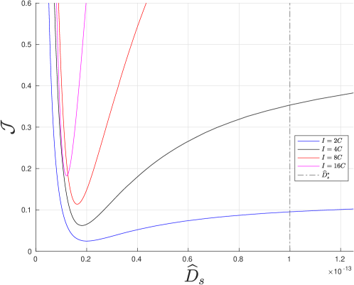
Figure 3: Dependence of the error functional $\mathcal{J}$ on the parameter $\widehat{D}_{s}$ in the SP model for the considered C-rates of 2C, 4C, 8C and 16C. The true value of the parameter $\widehat{D}^{*}_{s}=10^{-13}$ (m² s^-1) is indicated with a vertical line.

We now move on to present our solutions to the inverse problem (29)–(30) for the cSP model, where the inferred parameters are ${\mathbf{P}}=[\mathcal{B},\sigma_{s},\widehat{D},R,\widehat{D}_{s}]$. Because of the uncertainty inherent in these solutions, which will become evident shortly, it is impractical to solve the inverse problem directly by minimizing the error functional (29) using methods of numerical optimization. Instead, we adopt the Bayesian formulation introduced in Section 3 where Algorithm 1 is used to generate Markov chains consisting of a large number of samples ($K=10^{4}$). Each parameter sample ${\mathbf{P}}_{i}$, $i=1,\dots,K$, is associated with the corresponding value of the error functional ${\mathcal{J}}({\mathbf{P}}_{i})$. We recall that Algorithm 1 is designed to explore regions of the parameter space characterized by large values of the likelihood function (32). Samples in the Markov chains obtained for the different considered C-rates are shown in Figures 4(a–d). Since there are five inferred parameters, we visualize these results representing the parameters $\mathcal{B}$, $\sigma_{s}$ and $\widehat{D}$ in terms of the three Cartesian coordinates with the remaining two parameters $R$ and $\widehat{D}_{s}$ color-coded in terms of the red-green-blue (RGB) color scheme. The RGB color model represents different colors by adding weighted contributions, with weights varying between 0 and 1, of red, green and blue. In Figures 4(a–e) the weight of red is chosen as 1/2, whereas the weights of green and blue are proportional to the values of $R$ and $\widehat{D}_{s}$, as indicated in the color map shown in Figure 4(f) (due to this convention, red is the dominant color in Figures 4(a–e)). Moreover, the size of the symbols (circles) representing a given sample ${\mathbf{P}}_{i}$ is proportional to $1/{\mathcal{J}}^{2}({\mathbf{P}}_{i})$ such that parameter values producing better fits are shown with larger symbols and are therefore more visible (however, the proportionality constant is different for different C-rates, such that symbols of the same size in Figures 4(a–d) do not correspond to the same values of the error functional). Thus, the clouds of markers shown in these figures can be interpreted as approximations of the posterior probability distributions $\pi({\mathbf{P}}|{\widetilde{V}})$, cf. (31). In Figures 4(a–d) we also indicate the true values ${\mathbf{P}}^{*}$ of the parameters and for clarity they are also show separately in Figure 4(e). These results are complemented in Figure 5 by the PDFs of the different material parameters ${\mathbf{P}}=[\mathcal{B},\sigma_{s},\widehat{D},R,\widehat{D}_{s}]$ and of the error functional ${\mathcal{J}}({\mathbf{P}})$ obtained along the Markov chains for the different C-rates.

        

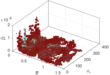
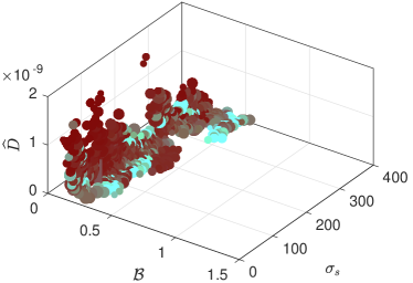
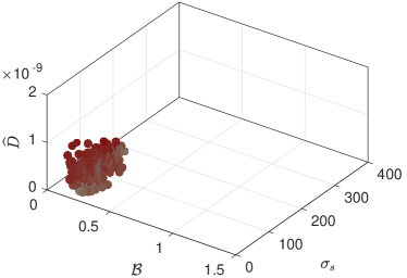
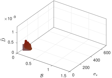
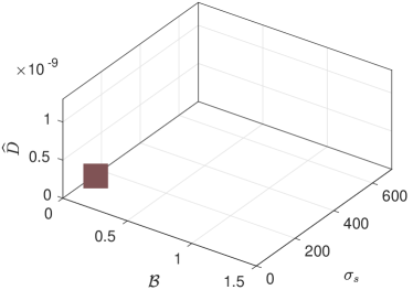
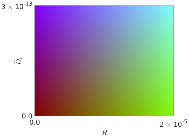
Figure 4: Approximations of the the posterior probability distribution $\pi({\mathbf{P}}|{\widetilde{V}})$, cf. (31), obtained in the Bayesian analysis of the inverse problem (29)–(30) for the C-rates of (a) 2C, (b) 4C, (c) 8C, (d) 16C. Symbols (circles) represents elements ${\mathbf{P}}_{i}$, $i=1,\dots,K$, of the Markov chains with the parameters $\{\mathcal{B},\sigma_{s},\widehat{D}\}$ represented in terms of the Cartesian coordinates and $\{R,\widehat{D}_{s}\}$ encoded using the color scale given in panel (f). The size of the symbols in panels (a)–(d) is proportional to $1/\mathcal{J}({\mathbf{P}}_{i})^{2}$ (with different proportionality constant in each panel). The true parameter values are denoted with a big cube and are also shown separately in panel (e).

     

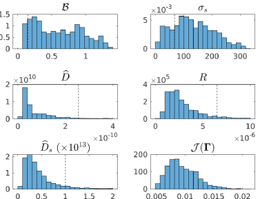
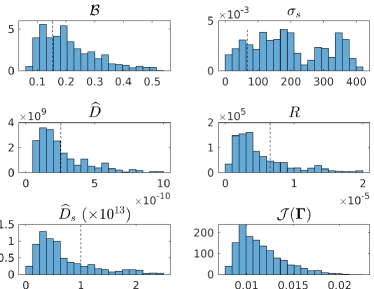
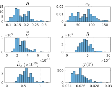
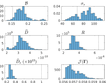
Figure 5: Probability density functions of the material parameters ${\mathbf{P}}=[\mathcal{B},\sigma_{s},\widehat{D},R,\widehat{D}_{s}]$ and of the error functional ${\mathcal{J}}({\mathbf{P}})$ obtained along the Markov chains for the different C-rates (a) 2C, (b) 4C, (c) 8C, (d) 16C.

The key observation to be made about the results shown in Figures 4 and 5 is that for decreasing C-rates the parameter values producing good fits are increasingly scattered which reflects the growing uncertainty of their reconstructions. For the C-rate of 2C, cf. Figure 4(a), these parameters values form a curved 2-dimensional “manifold” in the space spanned by $\{\mathcal{B},\sigma_{s},\widehat{D}\}$ where the parameters values differing by 300% or more may still give rise to equally accurate fits. For 4C, cf. Figure 4(b), the uncertainty of $\mathcal{B}$ is significantly reduced, but at the price of increasing the reconstruction uncertainty of the remaining parameters relative to the case with 2C, which is evident from comparing the PDFs in Figures 5(a) and 5(b). On the other hand, for large C-rates (8 and 16C) the obtained parameter values are clustered more closely reflecting reduced uncertainty of the reconstruction. However, for large C-rates the accuracy of the fits is also reduced as is evident from the PDFs of the error functional shown in the bottom right panels in Figures 5(a–d). The optimal values of the parameters reconstructed at large C-rates are further away from their true values than at low C-rates (except for the parameter $\sigma_{s}$ which is reconstructed rather well at high C-rates). This last observation is less evident from Figure 4, but can be deduced from the PDFs shown in Figure 5. Overall, these observations are consistent with what we found in the case of the SP model above.

At low C-rate the dominant contribution to the cell voltage is the that arising from the equilibrium overpotential of the LNC (hence the validity of the assumptions underpinning the SP and cSP models). Thus, at low C-rates, alterations to the values of the parameters $\{\mathcal{B},\sigma_{s},\widehat{D},R,\widehat{D}_{s}\}$ have a relatively small effect on the cell voltage, and this is manifested in the large spread of the clouds at low C-rates. Even though the cSP model better recovers the true value of $\widehat{D}_{s}$ than the SP model, it still consistently underestimates it. Moreover, at high C-rates, the size of the underestimation increases with C-rate and we speculate that this is for similar reasons to those described above for the SP model. The worsening of the match between the inferred and true values at 16C compared to 8C can be attributed to the breaking down of the assumptions underlying the cSP model (which require C-rates to not be too high); at 16C we are entering a regime where the cSP model does not accurately reproduce the discharge curves predicted by the DFN model. This is borne out by the results presented in [30].

           

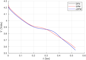
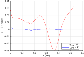
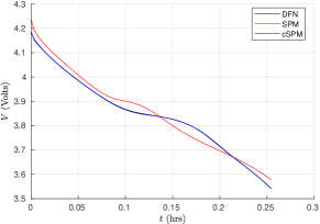
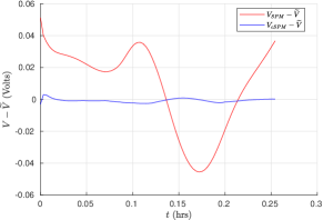
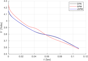
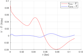
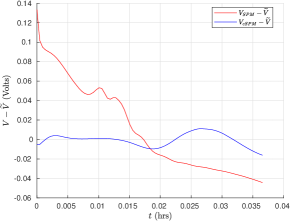
Figure 6: (Left column) Voltage curves obtained using the DFN model with the true parameters ${\mathbf{P}}^{*}$ and predicted by the SP and cSP models using optimal values of the reconstructed parameters for different C-rates (a)–(b) 2C, (c)–(d) 4C, (e)–(f) 8C, (g)–(h) 16C. The figures in the right column show the differences ${\widetilde{V}}(t)-V(t)$ of the voltage curves presented in the left column.

To finish the presentation of the results, in Figure 6 we compare the voltage curves obtained using the DFN model with true parameter values ${\mathbf{P}}^{*}$ and the voltage curves predicted by the SP and cSP models with optimal parameter values at different C-rates. These “optimal” sets of parameters are the elements of the Markov chains shown in Figures 4(a–d) which correspond to the smallest values of the error functional ${\mathcal{J}}({\mathbf{P}})$ (i.e., marked with the largest symbols in the figures). Figure 6 confirms that the voltage curves predicted by the cSP model are much closer to the “true” voltage curves than those obtained with the SP model, although the quality of the fits in both cases deteriorates as the C-rate increases. Moreover, the SP model tends to always overestimate the true voltage at early stages of the experiment.

5 Summary and Conclusions

In this study we have considered the inverse problem of parameterizing Newman-type models of lithium transport focusing on quantifying the inherent uncertainty of this process. In order to isolate intrinsic mechanisms responsible for this uncertainty, we have concentrated on an idealized problem where “synthetic” measurements are manufactured using the most complete DFN model with parameter values considered “true”, whereas parametrization is performed based on simplified versions of this model, namely, the SP and cSP models. By framing the problem in this way, we are able to eliminate aspects which affect uncertainty, but are hard to quantity such as, e.g., experimental errors.

Since the SP model involves one parameter only, the calibration problem can be solved in this case simply by plotting the error functional as a function of the unknown parameter $\widehat{D}_{s}$, cf. Figure 3. On the other hand, the cSP model involves five adjustable material parameters and the corresponding inverse problem is solved using the Bayesian approach where the reconstructed parameters are represented in terms of the posterior probability distributions quantifying the relative uncertainties of different values.

As a main finding of this study, we reveal an inherent trade-off between accuracy and uncertainty in the parametrization process. More specifically, when the C-rate is small, the two optimally parameterized simplified models fit the measurement data very well, although good fits are obtained with a broad range of parameters values thus making it hard to ascertain precise values of these parameters, cf. Figures 3–5. On the other hand, for large C-rates the best fits to measurements are obtained with more narrowly determined parameters, although the accuracy of these fits deteriorates. Moreover, while they are less uncertain, the parameter values inferred at higher C-rates tend to have larger errors with respect to the true values. Thus, one can conclude that, as C-rate increases, uncertainty of inverse modelling is traded for inaccuracy. These observations highlight the challenges involved in inferring unknown material properties via inverse modelling based on simplified models and voltage curves used as measurements. It is possible that these difficulties could be mitigated by using measurements of additional quantities in the parametrization process, such as, e.g., the concentration of lithium as was done in [21, 27, 36], although such measurements are usually much harder to obtain.

Our overall conclusions are that obtaining parameter values using simplified versions of the DFN model is a viable and useful strategy because these simplified models reduce the size of the parameter space and hence drastically reduce the computational effort required in the fitting process. However, care must be taken to make sure that the ranges of validity of the simplified models coincide with the operating regimes in which the experimental data was harvested. If this is not the case, we are essentially attempting to fit an invalid model and accurate results cannot be expected. Finally, higher C-rate data is more valuable for inverse modelling than low C-rate data because cell voltages are more strongly depend upon a variety of parameters (at low C-rates the cell voltage is almost entirely determined by $U_{eq}$) which allows us to reduce the amount of uncertainty in their reconstruction.

Appendix A Numerical Approach

In this appendix we provide some details concerning our approach to the numerical solution of the DFN, SP and cSP models, and the achieved levels of accuracy. This description focuses on the DFN model, but similar, suitably simplified, methods are also used to solve the SP and cSP models. Our numerical method consist of using (i) finite element approximation given in [42] for spatial discretization (in the macroscopic variable $x$) of the electrolyte equations (1)–(9), and also for the treatment of spatial discretization (in the microscopic variable $r$) of the microscopic equations (10)-(11) and (ii) and MATLAB’s ode15s routine for temporal integration. Approximation is both $x$ and $r$ is second-order accurate. First, to discretize the coordinate $x$, we introduce a set of points $x_{i}$, $i=0,\dots,N$ with step size $\Delta_{x}=x_{i+1}-x_{i}$ and denote the corresponding values of $c(x,t)$, $\Phi(x,t)$ and $\Phi_{s}(x,t)$ by $c_{i}(t)$, $\Phi_{i}(t)$ and $\Phi_{s,i}(t)$. At each of these grid points $x_{i}$ we need to determine the lithium concentration by solving equation (10). Discretizing the microscopic coordinate $r$ with $r_{j}=j\Delta_{r}$, where $\Delta_{r}=1/(M-1)$ for $j=1,\dots,M$, we have $N\times M$ different stations in $r$. We denote the values of lithium concentration at these locations by $c_{s,i}^{j}(t)$, where the index $i$ represents particle’s position in $x$ whereas $j$ represents radial position within the particle.

In total, we have $2N$ equations for the concentration and potential in the electrolyte, $N$ equations for the potential in the solid, and $M\times N$ equations for the concentration in the solid. Our solution vector thus consists of a total of $(3+M)\times N$ unknowns. We assemble the unknown functions of time into one large  vector ${\bf u}(t)$ as follows

$${\bf u}(t)=[c_{1},...,c_{N},\phi_{1},...,\phi_{N},\phi_{s1},...\phi_{sN},c_{s,1}^{1},...,c_{s,N}^{1},...,c_{s,1}^{M},...c_{s,N}^{M}]^{T}$$ (33)

$$=[{\bf c}(t),{\bf\Phi}(t),{\bf\Phi_{s}}(t),{\bf c_{s}}(t)]^{T}$$ (34)

where the subscript $T$ denotes the transpose. This leads us to the following system of DAEs

$${\bf{M}}\frac{d{{\bf u}}}{dt}={\bf f(u)},\qquad\text{with}\qquad{\bf u}|_{t=0}={\bf u}_{0}.$$ (35)

Here ${\bf M}_{{(3+M)\times N\times(3+M)\times N}}$ is the mass matrix whose entries are coefficients of the time derivatives and the function ${\bf f(u)}$ is non-linear and returns a vector of dimension $(3+M)\times N$. Its entries represent the right-hand side of the discretized equations. To solve this temporal system of DAEs we use ode15s from MATLAB.

As we have already mentioned in Section 2.3, solution of the cSP model consists of three steps. In the first step we solve the 1D diffusion equation (10) with boundary condition (11) and initial condition (12) in a representative electrode particle, which is the SP model (18)–(20). In the second step we solve the electrolyte equations (1)–(2) with boundary condition (8) and initial condition (12). Note that both these system of DAEs are solved independently. The first step (the SP model) requires a discretization in $r$ with $M$ grid points and the second step requires a discretization in $x$ with $N$ grid points. The dimensions of the DAEs systems that we need to integrate in time for the SP model, cSP model and DFN model are $M$, $2N+M$ and $(3+M)\times N$, respectively. It is clear that the cSP model is computationally more expensive than the SP model, but it is still very fast compared to the DFN model. For instance, for $M=50$ and $N=50$ the simulation time is 31 seconds for the DFN model, 0.32 seconds for the cSP model and $0.12$ seconds for the SP model. All these simulation have been performed on an Intel(R) Core(TM) i9-9880H CPU @ 2.30GHz.

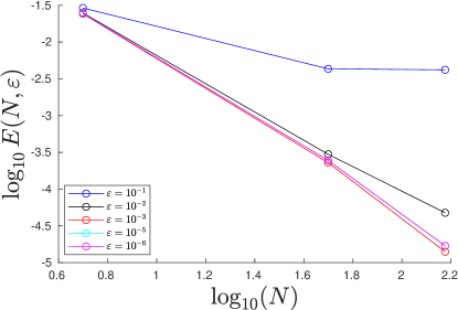
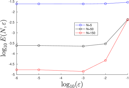
Figure 7: Dependence of the mean-square error (36) on (a) $N$ for different fixed $\varepsilon$ and (b) $\varepsilon$ for different fixed $N$.

The accuracy of the numerical solution is determined by the parameters $M$ and $N$ as well as the tolerance (both relative and absolute) of time integration $\varepsilon$ (which is used as a parameter by the function ode15s). These errors implicitly determine a lower bound on the error functional (29) below which this expression cannot be reduced, which in turn is needed to properly formulate the Bayesian inference problem in Section 3.. In order to estimate how this lower bound depends on the numerical parameters, we defined the quantity

$$E(N,\varepsilon)=\int_{0}^{t_{f}}|V_{DFN}(N_{0},\varepsilon_{0})-V_{DFN}(N,\varepsilon)|^{2}\,dt,$$ (36)

where $V_{DFN}(N,\varepsilon)$ is the voltage obtained by solving numerically the DFN system (1)–(11) using the numerical parameters $N$ and $\varepsilon$, whereas $N_{0}=500$ and $\varepsilon_{0}=10^{-6}$ are the most refined values of these parameters we consider. Thus, $V_{DFN}(N_{0},\varepsilon_{0})$ may be regarded as the “true” voltage and expression (36) as a mean-square error due to numerical approximation of the DFN system (1)–(11). The dependence of $E(N,\varepsilon)$ on $N$ with $\varepsilon$ fixed and on $\varepsilon$ with $N$ fixed in shown in Figures 7(a) and 7(b), respectively. Both these figures show the expected behavior with error (36) reduced as the numerical parameters $N$ and $\varepsilon$ are refined. Based on this data, we chose to perform our computations with $N=50$ and $\varepsilon=10^{-3}$ such that the corresponding inaccuracy in the evaluation of the error functional (29) can be conservatively estimated as $\mathcal{O}(10^{-3})$. This choice of the numerical parameters thus balances accuracy with computational cost.

References

- [1] G. E. Blomgren, J. Electrochem. Soc., 164(1), A5019 (2016).
- [2] W. Chen, J. Liang, Z. Yang, and G. Li, Energy Procedia, 158, 4363 (2019).
- [3] M. Doyle, J. Newman, A. S. Gozdz, C. N. Schmutz, and J. M. Tarascon, J. Electrochem. Soc., 143, 1890 (1996).
- [4] M. Doyle, T. F. Fuller, and J. Newman, J. Electrochem. Soc., 140, 1526 (1993).
- [5] T. F. Fuller, M. Doyle, and J. Newman, J. Electrochem. Soc., 141, 1 (1994).
- [6] V. Srinivasan and J. Newman, J. Electrochem. Soc., 151, A1517 (2004).
- [7] A. Harikesh and S. Onori, J. Electrochem. Soc., 166(8), A1380 (2019).
- [8] N. Jin, D. L. Danilov, P. M. Van den Hof, and M. C. Donkers, Int. J. Energy Res., 42(7), 2417 (2018).
- [9] S. A. Krachkovskiy, J. M. Foster, J. D. Bazak, B. J. Balcom, and G. R. Goward, J. Phys. Chem. C, 122(38), 21784 (2018).
- [10] A. Zulke, I. Korotkin, J. M. Foster, M. Nagarathinam, H. Hoster, and G. Richardson, submitted.
- [11] F. Ciucci and W. Lai, Transp. Porous Media, 88, 249 (2011).
- [12] G. Richardson, G. Denuault, and C. Please, J. Eng. Math., 72, 41 (2012).
- [13] J. M. Foster, A. Gully, H. Liu, S. Krachkovskiy, Y. Wu, S. Schougaard, M. Jiang, G. Goward, G. Botton, and B. Protas, J. Phys. Chem. C, 119, 12199 (2015).
- [14] A. A. Franco, RSC Adv., 3, 13027 (2013).
- [15] A. Jokar, B. Rajabloo, M. Désilets, and M. Lacroix, J. Power Sources, 327, 44 (2016).
- [16] M. Ecker, T. K. D. Tran, P. Dechent, S. Käbitz, A. Warnecke, and D. U. Sauer, J. Electrochem. Soc., 162, A1836 (2015).
- [17] M. Ecker, S. Käbitz, I. Laresgoiti, and D. U. Sauer, J. Electrochem. Soc., 162, A1849 (2015).
- [18] J. Schmalstieg and D. U. Sauer, J. Electrochem. Soc., 165(16), A3799 (2018).
- [19] J. Schmalstieg, C. Rahe, M. Ecker, and D. U. Sauer, J. Electrochem. Soc., 165(16), A3811 (2018).
- [20] M. Klett, M. Giesecke, A. Nyman, F. Hallberg, R. W. Lindström, G. Lindbergh, and I. Furó, J. Am. Chem. Soc., 134, 14654, (2012).
- [21] A. K. Sethurajan, S. Krachkovskiy, I. C. Halalay, G. R. Goward, and B. Protas, J. Phys. Chem. B, 119, 12238 (2015).
- [22] G. Richardson, J. M. Foster, A. K. Sethurajan, S. A. Krachkovskiy, I. C. Halalay, G. R. Goward, and B. Protas, J. Electrochem. Soc., 165, H561 (2018).
- [23] R. Smith, Uncertainty Quantification: Theory, Implementation, and Applications, Society for Industrial and Applied Mathematics, USA (2013).
- [24] L. Tenorio, An Introduction to Data Analysis and Uncertainty Quantification for Inverse Problems, Society for Industrial and Applied Mathematics, USA (2017).
- [25] J. Kaipio and E. Somersalo, Statistical and Computational Inverse Problems, Springer-Verlag New York, USA (2005).
- [26] A. K. Sethurajan, S. Krachkovskiy, G. Goward, and B. Protas, J. Comput. Chem., 40(5), 740 (2019).
- [27] A. K. Sethurajan, J. M. Foster, G. Richardson, S. A. Krachkovskiy, J. D. Bazak, G. R. Goward, and B. Protas, J. Electrochem. Soc., 166, A1591 (2019).
- [28] A. Aitio, S. Marquis, P. Ascencio, and D. Howey, arXiv (2020), arXiv:2001.09890
- [29] S. G. Marquis, V. Sulzer, R. Timms, C. P. Please, and S. J. Chapman, J. Electrochem. Soc., 166(15), A3693 (2019).
- [30] G. Richardson, I. Korotkin, R. Ranom, M. Castle, and J. M. Foster, Electrochim. Acta, 339, 1 (2020).
- [31] S. J. Moura, F. B. Argomedo, R. Klein, A. Mirtabatabaei, and M. Krstic, IEEE Trans. Control Sys. Technol., 25, 453 (2016).
- [32] M. Guo, G. Sikha, and R. E. White, J. Electrochem. Soc., 158(2), A122 (2010).
- [33] P. Kemper and D. Kum, IEEE VPPC, 158, (2013).
- [34] A. M. Bizeray, J.-H. Kim, S. R. Duncan, and D. A. Howey, IEEE Trans. Control Sys. Technol., 1 (2018).
- [35] I. R. Moyles, M. G. Hennessy, T. G. Myers, and B. R. Wetton, SIAM J. Appl. Math., 79(4), 1528 (2019).
- [36] J. Morales Escalante, W. Ko, J. M. Foster, S. Krachkovskiy, G. Goward, and B. Protas, Electrochim. Acta, 349, 136290 (2020).
- [37] A. M. Stuart, Acta Num., 19, 451, (2010).
- [38] B.V. Gnedenko and A.Y. Khinchin, An elementary introduction to the theory of probability, pp. 105–113, Dover, USA (1962).
- [39] S. Chib and E. Greenberg, Am. Stat., 49(4), 327 (1995).
- [40] N. Metropolis, A. Rosenbluth, M.Rosenbluth, A.Teller, and E. Teller, J. Chem. Phys., 21, 1087 (1953).
- [41] S. J. Press, Bayesian statistics: principles, models, and applications, Wiley, New York (1989).
- [42] I. Korotkin, S. Sahu, S. O’Kane, G. Richardson, and J. M. Foster, “DandeLiion v1: An extremely fast solver for the Newman model of lithium-ion battery (dis)charge”, arXiv:2102.06534v1, (2021).