Three-loop corrections to the muon and heavy quark decay rates

Abstract

Recently, $\mathcal{O}\left(\alpha^{3}\right)$ corrections to the muon decay rate and $\mathcal{O}\left(\alpha_{s}^{3}\right)$ to heavy quark decays have been determined by Fael, Schönwald, and Steinhauser. This is the first such perturbative improvement of these important quantities in more than two decades. We reveal and explain a symmetry pattern in these new corrections, and confirm the most technically difficult parts of their evaluation.

I Introduction

Muon decay provides one of the pillars of the Standard Model, the Fermi constant $G_{F}$ Marciano:1999ih . Its determination relies on precise measurements of the muon lifetime Webber:2010zf ; Tishchenko:2012ie and mass Nishimura:2020jjm , and on theoretical evaluation of radiative corrections. These corrections arise primarily from quantum electrodynamic (QED) interactions involving the muon and the daughter electron, and are expressed as a power series in the fine structure constant $\alpha\simeq 1/137$.

Very recently, a new term in this series has been calculated Fael:2020tow using an expansion in the difference of the muon and electron masses. Here we confirm the most demanding parts of the expansion published in Fael:2020tow . We also explain a pattern governing the first two terms of the expansion.

Determination of the coefficients of increasing powers of $\alpha$ requires monumental efforts. A new result appears very rarely, approximately once every one or two generations of theorists. Each new result is witness to a new technology available in perturbative quantum field theory. First order corrections, calculated in 1955 Behrends:1955mb , were in fact the first loop effects calculated for a decay process. They served as a model for subsequent studies of quantum chromodynamics (QCD) processes in heavy quark decays Jezabek:1988iv ; Czarnecki:1994pu .

It took more than 40 years before the second-order coefficient became known vanRitbergen:1999fi ; vanRitbergen:1998yd . That progress was made possible by the technique of recurrence relations based on integration-by-parts Chetyrkin:1981qh ; Tkachov:1981wb and on symbolic manipulations with computers vanRitbergen:1996ng .

Now, another two decades later, the coefficient of $\alpha^{3}$ has been determined Fael:2020tow . Several theoretical developments underly this advancement. Laporta algorithm Laporta:2001dd allows to express multi-loop integrals in terms of a relatively small number of master integrals. This algorithm can be implemented in powerful symbolic algebra software capable of parallelization Ruijl:2017dtg ; Smirnov:2019qkx . Finally, despite the electron being about 207 times lighter that the muon, the calculation is done as an expansion around the situation where the electron and the muon masses, $m_{e}$ and $m_{\mu}$, are equal Archambault:2004zs ; Czarnecki:1996gu ; Dowling:2008mc .

Historically, radiative corrections to the muon decay were calculated before corrections to heavy quark decays, because QCD was developed only later. Computational technology is the same in both QED and perturbative QCD, and once the QED corrections are known, it is relatively easy to evaluate additional diagrams involving multi-gluon vertices. Ref. Fael:2020tow presents corrections both for the muon and for the $b$-quark decays. Wherever our discussion below is relevant for both types of processes, we refer to the decaying particle’s mass as $M$, and denote the mass of the produced charged particle by $m$. We use $\delta=1-m/M$ to denote the expansion parameter: the relative difference of masses.

In Section II we present our calculation of five terms of the expansion in $\delta$ for a subset of corrections, including the most demanding part with all quanta (photons or gluons) coupling to incoming or outgoing fermions, rather than, for example, to virtual loops. In Section III we demonstrate how the first two terms in the expansion in $\delta$ can be found from a form factor, first determined in 2004 in Ref. Archambault:2004zs . Section IV contains our conclusions.

II Expansion in the mass difference

As we shall demonstrate in Section III, the first two terms of the expansion of the decay rate in the mass difference may be obtained without a new calculation. Unfortunately, the remainder of the expansion requires a challenging calculation. For this publication, we have evaluated the first five terms of the expansion, $\delta^{5,\dots,9}$ of the three most difficult contributions: those proportional to $C_{F}^{3}$, $C_{F}^{2}n_{b}$, and $C_{F}n_{b}^{2}$ where $n_{b}$ labels loops containing a fermion of mass $M$. (We use the standard notation for the SU($N$) factors: $C_{F}=(N^{2}-1)/(2N)$, $C_{A}=N$, $T_{F}=1/2$ with $N=3$ for QCD and $C_{F}=1$, $C_{A}=0$, $T_{F}=1$ for QED Muta:2010xua .) Our method, originally developed for corrections of $\mathcal{O}\left(\alpha^{2}\right)$ or $\mathcal{O}\left(\alpha_{s}^{2}\right)$ in Ref. Dowling:2008mc , is the same as the one employed in Ref. Fael:2020tow for $\mathcal{O}\left(\alpha_{s}^{3}\right)$ ($\alpha_{s}$ denotes the strong coupling constant). However, we used a different software implementation.

In this section we briefly describe our method using the example of the muon decay. It was found in Ref. Dowling:2008mc that an expansion in terms of $\delta$ is useful for computing high order corrections. In particular, the calculation is much less involved than an expansion around $m/M=0$, and converges very well all the way to the physical value of ${m_{c}/m_{b}}$ or ${m_{e}}/{m_{\mu}}$, even though $m_{e}/m_{\mu}=0.005$ is very far from the equal mass limit.

Our crucial tool is the optical theorem. It allows us to write contributions to the decay rate of the $b$-quark or muon as self energy diagrams. To generate the diagrams, we use DiaGen/IdSolver diagen modified to work with the types of propagators and expansions that appear in the present calculation. This code also produces the required integration by parts (IBP) identities and carries out the reduction to master integrals. The reduction of the large number of necessary integrals required the use of the WestGrid cluster which is part of the high performance computing infrastructure Compute Canada.

The decay is induced by an effective Fermi interaction with the $W$ boson contracted to a point, as shown in Fig. 1.

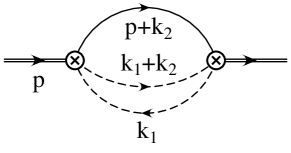
(a)                                                                    (b)

Figure 1: The tree level contribution to muon decay. Panel (a) shows the full amplitude with the $W$ boson. Panel (b) shows the muon self-energy diagram whose imaginary part we calculate to obtain the squared amplitude. Circled crosses indicate effective interactions obtained by neglecting the momentum dependence in $W$ propagators (Fermi interaction).

Corrections due to the $W$ propagator including electroweak effects are known up to two loops Awramik:2003ee . Here we are interested in three loop QED corrections in the limit of a heavy $W$. They are described by five loop self energy diagrams (the extra two loops are responsible for the tree-level decay in Fig. 1(b)). We show examples of such diagrams in Fig. 2.

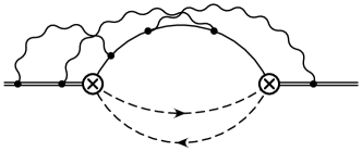
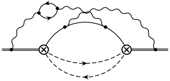
(a)                                                                (b)

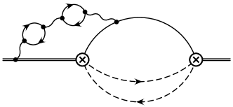
(c)

Figure 2: Examples of third-order radiative corrections to the muon decay. Wavy lines represent photons, contributing to both virtual and real radiation. In our approach, the imaginary part of such five loop diagrams is calculated.

The integral over the neutrino loop is carried out first by integrating over $k_{1}$ shown in Fig. 1(b). This can be done at any QED order because the neutrinos do not interact with each other in the approximation considered here. The number of loops is thus reduced by one, at the price of introducing a propagator with non-integer power. This complicates the IBP reduction.

For the remaining four loop integrals, we use an asymptotic expansion in $\delta$, which we now describe.

II.1 Asymptotic Expansion

General properties of the asymptotic expansion of the loop integrals can be explained with the help of Fig. 1. Since we have already integrated over the neutrino loop, we only need to consider $k_{2}$ when carrying out the expansion. The following integral remains

$$\int\frac{d^{d}k_{2}}{(2\pi)^{d}}\frac{1}{(k_{2}^{2})^{\epsilon}[(p+k_{2})^{2}-m^{2}]}=\int\frac{d^{d}k_{2}}{(2\pi)^{d}}\frac{1}{(k_{2}^{2})^{\epsilon}[k_{2}^{2}+2p\cdot k_{2}+M^{2}\delta(2-\delta)]}$$ (1)

where we use dimensional regularization with $d=4-2\epsilon$. Without QED corrections, there are two regions: soft with components $k_{2}$ of the order of $M-m$, thus much smaller than $M$; and hard with $k_{2}\sim M$. In the hard region, the term $M^{2}\delta(2-\delta)$ can be treated as small. After expanding in it, the integral takes the form

$$\int\frac{d^{d}k_{2}}{(2\pi)^{d}}\frac{1}{(k_{2}^{2})^{\epsilon}\left[k_{2}^{2}+2p\cdot k_{2}\right]}.$$ (2)

This is an on-shell self-energy integral with no imaginary part and so it does not contribute to the decay. This is the crucial observation which holds in any order in QED: if the momentum flowing through the neutrinos is large, the resulting integral has no imaginary part. This reduces the number of regions that must be considered by half. At $\mathcal{O}\left(\alpha^{3}\right)$ this means that we only need to consider eight regions instead of the general 16. Moreover, among the non-contributing regions is the computationally very difficult one with all five hard loops.

In the soft region, $k_{2}\sim\delta\cdot M$ and we simplify the integral in Eq. (1) by noticing that some terms are suppressed by an extra power of $\delta$,

$$\int\frac{d^{d}k_{2}}{(2\pi)^{d}}\frac{1}{(k_{2}^{2})^{\epsilon}[2p\cdot k_{2}+2M^{2}\delta+\underbrace{k_{2}^{2}-M^{2}\delta^{2}}_{\text{small}}]}.$$ (3)

Thus we encounter integrals with so called eikonal propagators Bagan:1992ty ; Czarnecki:1996nr whose general form is

$$\int\frac{d^{d}k}{(2\pi)^{d}}\frac{1}{(k^{2})^{n_{1}}[2p\cdot k]^{n_{2}}\left[2p\cdot k+\Delta\right]^{n_{3}}},$$ (4)

where $\Delta$ does not depend on the integration variable $k$. We have included another eikonal propagator that appears in higher-order loop diagrams. As it turns out, in all cases $\Delta$ takes the form of a constant or another eikonal propagator. This makes it possible to apply this integral iteratively when computing the required master integrals.

II.2 Master Integrals

Expansion in relevant momentum regions of all diagrams leads to a large number of eikonal and on-shell integrals. We encounter at most three-loop on-shell integrals because the four-loop on-shell integrals contribute only to the real part and not to the imaginary part that we need.

Fortunately the three-loop on-shell master integrals have been computed in Ref. Lee:2010ik to the required order in $\epsilon$ for the present calculation. We note that these integrals were originally computed in Ref. Laporta:1996mq in the context of the fermion anomalous magnetic moment, $(g-2)$, but it was not until Lee:2010ik that enough terms in the $\epsilon$ expansion where known to make the present calculation possible.

The soft integrals appear up to four loops. After reducing to master integrals, there are one one-loop, one two-loop, three three-loop and 13 four-loop master integrals that must be computed. The general one-loop eikonal integral in Eq. (4) is computed in Bagan:1992ty . The result has the property

$$\int\frac{d^{d}k}{(2\pi)^{d}}\frac{1}{(k^{2})^{n_{1}}[2p\cdot k]^{n_{2}}[2p\cdot k+\Delta]^{n_{3}}}\propto\Delta^{D-2n_{1}-n_{2}-n_{3}}.$$ (5)

As discussed in Section II.1, the form of $\Delta$ in this result makes it possible to iteratively apply the one loop computation to all two and three-loop and almost all four-loop eikonal type master integrals that are required. The remaining four-loop eikonal integrals can be computed analytically using a single Mellin-Barnes parameter. In all cases, the Mellin-Barnes integral can be evaluated by summing over the poles of the Gamma functions. Thus all eikonal integrals can be written explicitly in terms of Gamma and hypergeometric functions which are then expanded in $\epsilon$ to the needed order. For the expansion of hypergeometric functions, we use the Mathematica package HypExp Huber:2007dx . Detailed examples of evaluation of eikonal integrals can be found in Ref. Fael:2020njb ; Dowling:2012phd .

The final ingredient are the three-loop renormalization constants. The mass dependent constants are known in an expansion around the limit ${m/M}=0$ Bekavac:2007tk . We require the opposite expansion and thus had to compute the wave-function and mass renormalization terms. The calculation was done in an identical way to Bekavac:2007tk except, of course, expanding around $m/M=1$.

Interestingly, authors of Bekavac:2007tk were able to present their solution only in terms of one- and two-dimensional integrals which must be computed numerically. In the limit $m/M=1$ however, we obtain fully analytic results. [After this calculation was completed, we learned about Ref. Fael:2020bgs where analytic results in the limits $m/M=0,1,\infty$ are presented.]

Using the approach described in this section, we have been able to confirm terms in the first five orders, $\delta^{5},\dots,\delta^{9}$, of Ref. Fael:2020tow , in the most technically difficult groups: the ones that contain three photons, all coupling to the main muon-electron line, one example of which is shown in Fig. 2(a); and diagrams containing one or two virtual loops with mass $M$, as shown in Fig. 2(b,c).

In principle, an extension of our calculation to diagrams containing virtual $m$ loops and massless loops, and three-gluon vertices is possible. Instead, in the following Section III, we show how one can reproduce the first two terms of all types from already known form factors.

III Information from the zero-recoil form factor

III.1 Hidden symmetry under $M\leftrightarrow m$

The starting point of the expansion in the difference of masses is the equal mass limit. There, the three loop correction has been known for a long time Archambault:2004zs . That result can be used to obtain the first two terms in the mass difference expansion, as explained in Ref. Dowling:2008mc .

Without radiative corrections, the effect of the electron mass on the muon decay rate is known exactly,

$$\frac{\Gamma(\mu\to e\nu\bar{\nu})}{\Gamma_{0}}=1-8\rho^{2}+8\rho^{6}-\rho^{8}-24\rho^{4}\ln\rho,$$ (6)

where $\Gamma_{0}=\frac{G_{F}^{2}M^{5}}{192\pi^{3}}$ is the decay rate in the limit of a massless electron and $\rho=m/M$ is the ratio of electron and muon masses. Near the limit of equal electron and muon masses a useful parameter is $\delta=(M-m)/M=1-\rho$, introduced in Section II. The first two terms in the expansion of the tree-level decay rate around $\delta=0$ are

$$\frac{\Gamma(\mu\to e\nu\bar{\nu})}{\Gamma_{0}}=\delta^{5}-{3\over 2}\delta^{6}+\mathcal{O}\left(\delta^{7}\right).$$ (7)

We see that the phase space suppresses the decay rate by five powers of $\delta$.

The following discussion applies equally to the muon decay and to the semileptonic $b\to c$ and $b\to u$ quark decays. Quark decays require a more extensive calculation because QCD corrections have a richer gauge group structure. We therefore use the $b\to c$ decay as an example, use the language of QCD, and denote $\delta=(m_{b}-m_{c})/m_{b}$. Corrections to the muon decay can be deduced from a subset of results obtained for quarks.

We want to argue that when radiative corrections are included, the first two orders in $\delta$, displayed in Eq. (7), are affected only by virtual corrections and not by the real radiation. Real radiation emission is suppressed by two powers of the daughter fermion velocity in the rest frame of the decaying fermion. That velocity, $v=\sqrt{1-{m_{c}^{2}\over m_{b}^{2}}}$, is at most about $\delta$. So, the real radiation affects the decay rate only in the third order in the expansion, $\delta^{7}$.

It has also been demonstrated that the form factors arising from virtual corrections do not have a linear term in the $\delta$ expansion Dowling:2008mc , as long as the coupling constant $\alpha_{s}$ is renormalized in the symmetric point $\mu^{2}=m_{c}m_{b}$. This is because of the symmetry of the virtual gluon diagrams under the interchange $m_{b}\leftrightarrow m_{c}$. We have therefore used Eq. (7) to reproduce the first two terms of the expansion in Fael:2020tow .

The available information about the form factors in Archambault:2004zs is limited to the axial form factor. Fortunately, in the limit of equal masses, the vector form factor does not receive radiative corrections. Corrections are suppressed by the square of momentum transfer $q^{2}=(p_{b}-p_{c})^{2}$ which contributes again only in the third order, $\delta^{7}$.

Since the results of Archambault:2004zs assume the exact equal mass limit, they do not differentiate between the two heavy fermions. In Ref. Fael:2020tow effects of $b$ and $c$ loops are labeled with factors $n_{b}$ and $n_{c}$, to indicate that they are proportional to the number of those quarks in virtual loops (in reality of course there is $n_{b}=n_{c}=1$). We thus replace $n_{b}$ and $n_{c}$ in the formulas of Fael:2020tow by $N_{H}/2$, so that the number of heavy fermions $N_{H}$ in Archambault:2004zs corresponds to $n_{b}+n_{c}$.

Finally, when we apply Eq. (7), we obtain corrections in terms of the coupling constant normalized at the geometric mean of the decaying and daughter fermion. On the other hand, results of Ref. Fael:2020tow use the mass of the decaying fermion as the renormalization scale. To remedy this, we run the coupling constant in the formulas resulting from Eq. (7) using Kniehl:2002br ,

$$\frac{\alpha_{s}(m_{b}m_{c})}{\pi}= \frac{\alpha_{s}(m_{b}^{2})}{\pi}\left[1+\frac{\alpha_{s}(m_{b}^{2})}{\pi}\beta_{0}\delta+\left(\frac{\alpha_{s}}{\pi}\right)^{2}\delta\left(\beta_{0}^{2}\delta+\beta_{1}\right)\right],$$ (8)

$$\beta_{0}= {1\over 4}\left({11\over 3}C_{A}-{4\over 3}T_{F}n_{f}\right),$$ (9)

$$\beta_{1}= {1\over 16}\left({34\over 3}C_{A}^{2}-{20\over 3}C_{A}T_{F}n_{f}-4C_{F}T_{F}n_{f}\right),$$ (10)

where $n_{f}=n_{l}+N_{H}$. In the above formulas, $\delta$ originates from the logarithm $\ln{m_{b}\over m_{c}}=-\ln(1-\delta)=\delta+\mathcal{O}\left(\delta^{2}\right)$.

After this adjustment of the coupling constant in the axial form factor, we reproduce all coefficients of $\delta^{5}$ and $\delta^{6}$ in Ref. Fael:2020tow .

III.2 Example of the pattern in terms $\delta^{5}$ and $\delta^{6}$

As an example of the procedure outlined above, we consider the first two terms in the color part proportional to $C_{F}C_{A}^{2}$. In the Supplementary Material of Ref. Fael:2020tow these terms read $C_{F}C_{A}^{2}\left(d_{5}\delta^{5}+d_{6}\delta^{6}\right)$, with

$$d_{5} =-{16241\over 270}-{512\over 15}a_{4}-{64\over 45}\ln^{4}2-{1423\over 90}\pi^{2}+{1112\over 45}\pi^{2}\ln 2-{40\over 9}\pi^{2}\ln^{2}2+{194\over 675}\pi^{4}+{86\over 3}\zeta_{3}+{22\over 15}\pi^{2}\zeta_{3}-32\zeta_{5},$$ (11)

$$d_{6} ={1745\over 36}+{256\over 5}a_{4}+{32\over 15}\ln^{4}2+{1247\over 60}\pi^{2}-{156\over 5}\pi^{2}\ln 2+{20\over 3}\pi^{2}\ln^{2}2-{97\over 225}\pi^{4}-{259\over 5}\zeta_{3}-{11\over 5}\pi^{2}\zeta_{3}+48\zeta_{5},$$ (12)

where $a_{4}=\text{Li}_{4}(1/2)\simeq 0.517$ lewin and $\zeta_{n}$ is the Riemann zeta function NISTHandbook . Following the discussion around Eq. (7), the bulk of these terms should have the form $d_{5}\delta^{5}(1-3\delta/2)$. Consider the deviation from that pattern, $D=d_{6}+3d_{5}/2$,

$$D=-{1879\over 45}-{44\over 5}\zeta_{3}-{44\over 15}\pi^{2}+{88\over 15}\pi^{2}\ln 2,$$ (13)

a much simpler expression than either $d_{5}$ or $d_{6}$, but not zero.

We now show how this difference is removed by changing the renormalization scale. To this end, consider one- and two-loop form factor Shifman:1987rj ; Paschalis:1982zq ; Close:1984ad ; Czarnecki:1996gu , as summarized in Archambault:2004zs ,

$$\eta_{A}(\delta\to 0) =1+\eta_{A}^{(1)}{\alpha_{s}(m_{b}m_{c})\over\pi}+\eta_{A}^{(2)}\left(\alpha_{s}(m_{b}m_{c})\over\pi\right)^{2}+\mathcal{O}\left(\alpha_{s}^{3}\right),$$ (14)

$$\eta_{A}^{(1)}(\delta\to 0) =-{C_{F}\over 2\pi}$$ (15)

$$\eta_{A}^{(2)}(\delta\to 0) =C_{F}C_{A}\left(-{143\over 144}-{1\over 4}\zeta_{3}+{1\over 6}\pi^{2}\ln 2-{1\over 12}\pi^{2}\right)+\dots,$$ (16)

where we have neglected other color structures in $\eta_{A}^{(2)}$. Change of the scale of $\alpha_{s}$ in the square of the form factor produces an additional contribution $\alpha_{s}^{3}C_{F}C_{A}^{2}$,

$${48\over 5}\eta_{A}^{2} \to{96\over 5}\left[\eta_{A}^{(1)}\beta_{1}+2\eta_{A}^{(2)}\beta_{0}\right]$$ (17)

$$\to{96\over 5}\left[-{1\over 2}\cdot{17\over 24}+2{11\over 12}\left(-{143\over 144}-{1\over 4}\zeta_{3}+{1\over 6}\pi^{2}\ln 2-{1\over 12}\pi^{2}\right)\right]=D,$$ (18)

where the factor $48/5$ is related to the normalization of the results in Fael:2020tow . The result of changing the scale from the symmetric point $m_{b}m_{c}$ to $m_{b}^{2}$, given by Eq. (18), provides precisely the deviation from the pattern $d_{5}\delta^{5}(1-3\delta/2)$ we found in Eq. (13).

IV Conclusions

The third order correction to the muon and the heavy quark decay rates found in Ref. Fael:2020tow is an important milestone in perturbative quantum field theory. Here we have confirmed the first five terms of the three technically most difficult structures involving no light vacuum polarization loops and no three-gluon couplings. We have also revealed a pattern in the first two terms of the expansion of all flavor and color structures, hidden when the symmetry between the initial and the final fermion is broken by renormalization. This pattern becomes visible when a symmetric scale $Mm$ is used to renormalize the coupling.

We close by congratulating the authors of Ref. Fael:2020tow on completing their heroic calculation.

- (1) W. J. Marciano, Fermi Constants and “New Physics”, Phys. Rev. D60, 093006 (1999), eprint hep-ph/9903451.
- (2) D. Webber et al., Measurement of the positive muon lifetime and determination of the Fermi constant to part-per-million precision, Phys. Rev. Lett. 106, 041803 (2011).
- (3) V. Tishchenko et al., Detailed Report of the MuLan Measurement of the Positive Muon Lifetime and Determination of the Fermi Constant, Phys. Rev. D87, 052003 (2013), eprint 1211.0960.
- (4) S. Nishimura, H. A. Torii, Y. Fukao, T. U. Ito, M. Iwasaki, S. Kanda, K. Kawagoe, D. Kawall, N. Kawamura, N. Kurosawa, Y. Matsuda, T. Mibe, Y. Miyake, N. Saito, K. Sasaki, Y. Sato, S. Seo, P. Strasser, T. Suehara, K. S. Tanaka, T. Tanaka, J. Tojo, A. Toyoda, Y. Ueno, T. Yamanaka, T. Yamazaki, H. Yasuda, T. Yoshioka, and K. Shimomura, Rabi-Oscillation Spectroscopy of the Hyperfine Structure of Muonium Atoms (2020), eprint 2007.12386.
- (5) M. Fael, K. Schönwald, and M. Steinhauser, Third order corrections to the semi-leptonic and the muon decays (2020), to be published, eprint 2011.13654.
- (6) R. E. Behrends, R. J. Finkelstein, and A. Sirlin, Radiative corrections to decay processes, Phys. Rev. 101, 866 (1956).
- (7) M. Jeżabek and J. H. Kühn, QCD Corrections to Semileptonic Decays of Heavy Quarks, Nucl. Phys. B314, 1–6 (1989).
- (8) A. Czarnecki and M. Jeżabek, Distributions of leptons in decays of polarized heavy quarks, Nucl. Phys. B 427, 3–21 (1994), eprint hep-ph/9402326.
- (9) T. van Ritbergen and R. G. Stuart, On the precise determination of the Fermi coupling constant from the muon lifetime, Nucl. Phys. B564, 343 (2000), eprint hep-ph/9904240.
- (10) T. van Ritbergen and R. G. Stuart, Complete two loop quantum electrodynamic contributions to the muon lifetime in the Fermi model, Phys. Rev. Lett. 82, 488 (1999), eprint hep-ph/9808283.
- (11) K. G. Chetyrkin and F. V. Tkachev, Integration by parts: the algorithm to calculate -functions in 4 loops, Nucl. Phys. B192, 159–204 (1981).
- (12) F. V. Tkachov, A Theorem On Analytical Calculability Of Four Loop Renormalization Group Functions, Phys. Lett. B100, 65–68 (1981).
- (13) T. van Ritbergen, Perturbative QCD contributions to inclusive processes, Ph.D. thesis, Amsterdam U. (1996).
- (14) S. Laporta, High-precision calculation of multi-loop Feynman integrals by difference equations, Int. J. Mod. Phys. A15, 5087–5159 (2000), eprint hep-ph/0102033.
- (15) B. Ruijl, T. Ueda, and J. Vermaseren, FORM version 4.2 (2017), arXiv:1707.06453.
- (16) A. V. Smirnov and F. S. Chuharev, FIRE6: Feynman Integral REduction with Modular Arithmetic, Comput. Phys. Commun. 247, 106877 (2020), eprint 1901.07808.
- (17) J. P. Archambault and A. Czarnecki, Three-loop QCD corrections and b-quark decays, Phys. Rev. D70, 074016 (2004), eprint hep-ph/0408021.
- (18) A. Czarnecki, Two-loop QCD corrections to transitions at zero recoil, Phys. Rev. Lett. 76, 4124–4127 (1996), eprint hep-ph/9603261.
- (19) M. Dowling, J. H. Piclum, and A. Czarnecki, Semileptonic decays in the limit of a heavy daughter quark, Phys. Rev. D78, 074024 (2008), eprint 0810.0543.
- (20) T. Muta, Foundations of Quantum Chromodynamics: An Introduction to Perturbative Methods in Gauge Theories, World Scientific, Singapore, 3rd edition (2010).
- (21) M. Czakon, DiaGen/IdSolver, unpublished software.
- (22) M. Awramik and M. Czakon, Complete two loop electroweak contributions to the muon lifetime in the standard model, Phys. Lett. B568, 48–54 (2003), eprint hep-ph/0305248.
- (23) E. Bagan, P. Ball, and P. Gosdzinsky, The Isgur-Wise function to from sum rules in the heavy quark effective theory, Phys. Lett. B 301, 249–256 (1993), eprint hep-ph/9209277.
- (24) A. Czarnecki and V. A. Smirnov, Threshold behavior of Feynman diagrams: The master two-loop propagator, Phys. Lett. B394, 211–217 (1997), eprint hep-ph/9608407.
- (25) R. N. Lee and V. A. Smirnov, Analytic Epsilon Expansions of Master Integrals Corresponding to Massless Three-Loop Form Factors and Three-Loop g-2 up to Four-Loop Transcendentality Weight, JHEP 02, 102 (2011), eprint 1010.1334.
- (26) S. Laporta and E. Remiddi, The Analytical value of the electron at order in QED, Phys. Lett. B379, 283–291 (1996), eprint hep-ph/9602417.
- (27) T. Huber and D. Maitre, HypExp 2, Expanding Hypergeometric Functions about Half-Integer Parameters, Comput. Phys. Commun. 178, 755–776 (2008), eprint 0708.2443.
- (28) M. Fael, K. Schönwald, and M. Steinhauser, Relation between the and the kinetic mass of heavy quarks, Phys. Rev. D 103, 014005 (2021), eprint 2011.11655.
- (29) M. Dowling, High Order Corrections to Fundamental Constants, Ph.D. thesis, University of Alberta, Edmonton (2012), URL: https://era.library.ualberta.ca/items/67a8d114-09c6-4692-8deb-51072adb8fc8.
- (30) S. Bekavac, A. Grozin, D. Seidel, and M. Steinhauser, Light quark mass effects in the on-shell renormalization constants, JHEP 10, 006 (2007), eprint 0708.1729.
- (31) M. Fael, K. Schönwald, and M. Steinhauser, Exact results for and with two mass scales and up to three loops, JHEP 10, 087 (2020), eprint 2008.01102.
- (32) B. A. Kniehl, A. A. Penin, V. A. Smirnov, and M. Steinhauser, Potential NRQCD and heavy quarkonium spectrum at next-to-next-to-next-to-leading order, Nucl. Phys. B 635, 357–383 (2002), eprint hep-ph/0203166.
- (33) L. Lewin, Polylogarithms and associated functions, North Holland, New York (1981).
- (34) F. W. J. Olver, D. W. Lozier, R. F. Boisvert, and C. W. Clark, editors, NIST Handbook of Mathematical Functions, Cambridge University Press, Cambridge (2011).
- (35) M. A. Shifman and M. B. Voloshin, On Production of and Mesons in Meson Decays, Sov. J. Nucl. Phys. 47, 511 (1988).
- (36) J. E. Paschalis and G. J. Gounaris, Meson Decays in the Nonrelativistic Quark Model, Nucl. Phys. B 222, 473 (1983), [Erratum: Nucl. Phys. B 538, 532–532 (1999)].
- (37) F. E. Close, G. J. Gounaris, and J. E. Paschalis, The Ratio in the Quark Model, Phys. Lett. B 149, 209–212 (1984).