Relative polar curves and Monodromy

Abstract.

We show that given any germ of complex analytic function $f\colon(X,x)\to(\mathbb{C},0)$ on a complex analytic space $X$, there exists a geometric local monodromy without fixed points, provided that $f\in\mathfrak{m}_{X,x}^{2}$, where $\mathfrak{m}_{X,x}$ is the maximal ideal of $\mathcal{O}_{X,x}$. This result generalizes a well-known theorem of the second named author when $X$ is smooth at $x$ and it also implies the A’Campo theorem that the Lefschetz number of the monodromy is equal to zero. Moreover, we give an application to the case that $X$ has maximal rectified homotopical depth at $x$ and show that a family of such functions with isolated critical points and constant total Milnor number has no coalescing of singularities.

Introduction

In [20] J. Milnor proved that for any germ of complex function:

$$f:({\mathbb{C}}^{n+1},x)\to({\mathbb{C}},0)$$

one can associate a smooth locally trivial fibration for $1\gg\varepsilon>0$:

$$\varphi_{\varepsilon}:{\mathbb{S}}_{\varepsilon}(x)-f^{-1}(0)\rightarrow{\mathbb{S}}^{1}$$

induced by $f/|f|$, where ${\mathbb{S}}_{\varepsilon}(x)$ is the sphere centered at $x$ with radius $\varepsilon$ and ${\mathbb{S}}^{1}$ is the circle of radius $1$ of ${\mathbb{C}}$ centered at the origin.

In [7] H. Hamm made the observation that, when $x$ is an isolated critical point of $f$, the fibration of Milnor is isomorphic to the local fibration, for $1\gg\varepsilon\gg\eta>0$:

$$\psi_{\varepsilon,\eta}:\mathaccent 28695{B}_{\varepsilon}(x)\cap f^{-1}({\mathbb{S}}_{\eta})\rightarrow{\mathbb{S}}_{\eta}$$

induced by $f$, where $\mathaccent 28695{B}_{\varepsilon}(x)$ is the open ball centered at the point $x$ with radius $\varepsilon$.

From the work of [9] the hypothesis of isolated singularity can be lifted. Moreover the proper map:

$$\overline{\psi}_{\varepsilon,\eta}:B_{\varepsilon}(x)\cap f^{-1}({\mathbb{S}}_{\eta})\rightarrow{\mathbb{S}}_{\eta}$$

is a locally trivial fibration.

Milnor’s fibration leads to a notion of monodromy associated to $f$ at $x$. Precisely let $\varphi:X\rightarrow{\mathbb{S}}^{1}$ be a proper locally trivial smooth fibration. One can build on $X$ a smooth vector field $v$ which lifts the unit vector field tangent to ${\mathbb{S}}^{1}$. The integration of this vector field defines a smooth morphism $h:F\to F$ of a fiber of $\varphi$ onto itself that we call a geometric monodromy of $\varphi$. A geometric monodromy is not uniquely defined, but one can prove that its isotopy class is unique. Therefore there is an isomorphism induced by a geometric monodromy of $\varphi$ on the homology (or cohomology) of the fiber $F$ called the monodromy of $\varphi$.

In the case of Milnor’s fibration one often use the terminology of local geometric monodromy and local monodromy of $f$ at the point $x$.

In [15] the second named author gave a proof of the fact that for any germ of complex analytic function:

$$f:({\mathbb{C}}^{n+1},x)\to({\mathbb{C}},0)$$

having a critical point at $x$, there is a local geometric monodromy of $f$ at $x$ without fixed points.

By a well-known theorem of S. Lefschetz (see e.g. [10, p. 179]) this result implies that the local monodromy of $f$ at $x$ has a Lefschetz number equal to $0$. In fact, in [1], A’Campo showed that the Lefschetz number is zero in a more general situation, with heavy mathematical machinery, and attributed the proof of this theorem to P. Deligne.

Let $(X,x)$ be any germ of complex analytic space and denote by ${\mathfrak{m}}_{X,x}$ the the maximal ideal of the local ring $\mathcal{O}_{X,x}$ of germs of analytic functions of $X$ at $x$.

Theorem 0.1 (cf. [1]).

Let $f\colon(X,x)\to({\mathbb{C}},0)$ be a germ of complex analytic function such that $f\in{\mathfrak{m}}^{2}_{X,x}$. Then the local monodromy of $f$ at $x$ has Lefschetz number equal to $0$.

In this note we give the following generalization of Lê’s theorem, which in particular implies Theorem 0.1:

Theorem 0.2.

Let $f\colon(X,x)\to({\mathbb{C}},0)$ be a germ of complex analytic function such that $f\in{\mathfrak{m}}^{2}_{X,x}$. Then there is a local geometric monodromy of $f$ at $x$ which does not fix any point.

As in [15], the proof of Theorem 0.2 uses the notion of relative polar curve, which is due essentially to R. Thom. When $X=\mathbb{C}^{n+1}$ we first choose a sufficiently small open neighbourhood $U$ of $x$. For almost all linear function $\ell:{\mathbb{C}}^{n+1}\to{\mathbb{C}}$, one has that the critical space of the restriction $\left.(\ell,f)\right|_{U-\{f=0\}}$ is either always empty or a non-singular curve. When it is non-empty, we call the closure of the critical space of $\left.(\ell,f)\right|_{U-\{f=0\}}$ the relative polar curve $\Gamma_{\ell}(f,x)$ of $f$ at $x$ with respect to $\ell$.

The remarkable property of the relative polar curve is that, when $f$ has a critical point at $x$, its image by $\left.(\ell,f)\right|_{U}$ is empty or a curve that Thom called the Cerf’s diagram, which is tangent to the axis of values of $\ell$ (see e.g. [18, Proposition 6.6.5]). We show in Section 1 how to adapt this construction to the case that $X$ is singular at $x$ by taking a Whitney stratification. The condition that $f\in{\mathfrak{m}}^{2}_{X,x}$ is used here in order to prove that the Cerf’s diagram is tangent to the $\ell$-axis.

Associated with the Cerf’s diagram we have the carousel, a construction which again appears in [15]. This is a vector field $\omega$ over a small enough solid torus $D\times\partial D_{\eta}$ centered at the origin in $\mathbb{C}\times\mathbb{C}$ such that:

1. its projection onto the second component gives a tangent vector field over $\partial D_{\eta}$ of length $\eta$ and positive direction (called in [15] the unitary vector field of $\partial D_{\eta}$),

2. its restriction to $\left\{0\right\}\times\partial D_{\eta}$ is indeed the unitary vector field,

3. for every component of the Cerf’s diagram with reduced equation $\delta_{\alpha}=0$, $\omega$ is tangent to every $\delta_{\alpha}=\epsilon$ with $\epsilon$ small enough, and

4. the only integral curve that is closed after a loop in $\partial D_{\eta}$ is $\left\{0\right\}\times\partial D_{\eta}$.

Now we can use techniques of stratification theory to lift the carousel $\omega$ and obtain a stratified vector field on $X$ which is globally integrable. The integral curves of this vector field define a local geometric monodromy of $f$ at $x$ and of its restriction to $X\cap\{\ell=0\}$, defined on section 2. By condition (iv), the fixed points of the monodromy of $f$ can appear only on $X\cap\{\ell=0\}$. Thus, the proof of Theorem 0.2 follows by induction on the dimension of $X$ at $x$.

We give an example that the condition that $f\in{\mathfrak{m}}^{2}_{X,x}$ is necessary, even if $f$ has critical point at $x$ in the stratified sense. In the last section, we also extend a well-known theorem of the second named author (see [14]) about no coalescing of families of functions with isolated critical points and constant total Milnor number. The extension works when we consider functions on spaces with maximal rectified homotopical depth (also called spaces with Milnor property in [8]).

1. Relative polar curves

Let $f:(X,x)\to({\mathbb{C}},0)$ be the germ of a complex analytic function. We still call $f:X\to{\mathbb{C}}$ a representative of this germ. Let ${\mathcal{S}}=(S_{\alpha})_{\alpha\in A}$ be a Whitney stratification of a sufficiently small representative ${X}$ of $(X,x)$. We can assume that $x$ is in the closure $\overline{S}_{\alpha}$ of all the strata $S_{\alpha}$. So, the set of indices $A$ is finite.

Using [17, Lemme 21 §3] one can prove that there is a non-empty open Zariski subset $\Omega_{\alpha}$ of the affine functions such that, for every $\ell$ in $\Omega_{\alpha}$, $\ell(x)=0$ and the critical locus $C_{\alpha}$ of the restriction $\left.(\ell,f)\right|_{S_{\alpha}-f^{-1}(0)}$ of the function induced by $(\ell,f)$ on the space $S_{\alpha}-f^{-1}(0)$ is either always empty or a non-singular curve. Then, the closure $\Gamma_{\alpha}$ of $C_{\alpha}$ in ${X}$ is either empty or a reduced curve.

Definition 1.1.

For $\ell\in\cap_{\alpha\in A}\Omega_{\alpha}$ the union $\cup_{\alpha\in A}\Gamma_{\alpha}$ is either empty or a reduced curve. This curve is called the relative polar curve $\Gamma_{\ell}(f,{\mathcal{S}},x)$ of $f$ at $x$ relatively to $\ell$ and the stratification ${\mathcal{S}}$ of $X$.

Remark 1.2.

Notice that if the stratum $S_{\alpha}$ has dimension one, the whole stratum $S_{\alpha}$ is critical and $\Gamma_{\alpha}$ is the closure $\overline{S}_{\alpha}$. In this case, since $S_{\alpha}$ is connected, $\Gamma_{\alpha}$ is a branch of the curve $\Gamma_{\ell}(f,{\mathcal{S}},x)$ at $x$, i.e. an analytically irreducible curve at $x$.

Using [17, Lemme 21 §3] we can also show that one can choose the $\Omega_{\alpha}$’s such that the restriction $\left.(\ell,f)\right|_{\Gamma_{\alpha}}$ is finite for any $\alpha\in A$.

A theorem of Remmert implies that the image of $\Gamma_{\alpha}$ by $\left.(\ell,f)\right.$ is a curve $\Delta_{\alpha}$, for any $\alpha\in A$.

We define:

Definition 1.3.

The union $\cup_{\alpha\in A}\Delta_{\alpha}$ is either empty or a reduced curve. This curve is called the Cerf’s diagram $\Delta_{\ell}(f,{\mathcal{S}},x)$ of $f$ at $x$ relatively to $\ell$ and the stratification ${\mathcal{S}}$.

When the stratification ${\mathcal{S}}$ is fixed, we shall speak of the relative polar curve $\Gamma_{\ell}(f,x)$ and the Cerf’s diagram $\Delta_{\ell}(f,x)$ without mentioning the stratification ${\mathcal{S}}$. But the reader must be aware that the notion of polar curve and Cerf’s diagram depends on the choice of the stratification.

We shall go back and forth between the case $(\mathbb{C}^{n+1},x)$ and the general case of germs of reduced analytic spaces $(X,x)$ and compare them to generalize what we have in [15]. For example, if $(X,x)=({\mathbb{C}}^{n+1},x)$, we can consider a Whitney stratification which has only one stratum. In [15], we have seen that the emptiness of $\Gamma_{\ell}(f,x)$ means that the Milnor fiber of $f$ at $x$ is diffeomorphic to the product of the Milnor fiber of $\left.f\right|_{\{\ell=0\}}$ at $x$ with an open disc, hence the local geometric monodromy of $f$ at $x$ is induced by the product of the local geometric monodromy of $\left.f\right|_{\{\ell=0\}}$ at $x$ and the identity of the open disc.

Also, for a germ of complex analytic function $f:(X,x)\to({\mathbb{C}},0)$, in general, we may suppose that the hyperplane $\{\ell=0\}$ is transverse to all the strata of the Whitney stratification ${\mathcal{S}}$ and it induces a Whitney stratification on ${X}\cap\{\ell=0\}$. Then, using the same arguments of [17], we can prove the following:

Proposition 1.4.

If, for a general linear form $\ell$ at $x$, the relative polar curve $\Gamma_{\ell}(f,x)$ is empty, there is a stratified homeomorphism of the Milnor fiber of $f$ at $x$ and the product with an open disc with the Milnor fiber of the restriction $\left.f\right|_{{X}\cap\{\ell=0\}}$ at $x$.

The proof of this proposition is based on the techniques Mather used to prove the Thom-Mather first isotopy lemma, cf. [19, 6]. We will outline these techniques in the next section and use them later.

Now observe that when $(X,x)=({\mathbb{C}}^{n+1},x)$ the point $x$ is a critical point of $f$ if and only if $f\in{\mathfrak{m}}_{{\mathbb{C}}^{n+1},x}^{2}$, where ${\mathfrak{m}}_{{\mathbb{C}}^{n+1},x}$ is the maximal ideal of the local ring ${\mathcal{O}}_{{\mathbb{C}}^{n+1},x}$. In the case of a germ of complex analytic function on $(X,x)$, the hypothesis $f\in{\mathfrak{m}}_{X,x}^{2}$, where ${\mathfrak{m}}_{X,x}$ is the maximal ideal of ${\mathcal{O}}_{X,x}$, replaces the condition that $f$ is critical at $x$. In fact, a key result for the proof of Theorem 0.2 is:

Proposition 1.5.

For a sufficiently general linear form $\ell$, if $f\in{\mathfrak{m}}_{X,x}^{2}$, the Cerf’s diagram $\Delta_{\ell}(f,x)$ is tangent at the point $(0,0)$ to the first axis, the image by $(\ell,f)$ of $\{f=0\}$.

Proof.

Of course, we have a Whitney stratification ${\mathcal{S}}=(S_{\alpha})_{\alpha\in A}$ on a sufficiently small representative of the germ $(X,x)$. We may assume that $x$ is the closure of all the strata.

It is enough to prove the proposition for the image $\Delta_{\alpha}$ of $\Gamma_{\alpha}$ by $(\ell,f)$, for each $\alpha\in A$.

In [15], it was considered that $\ell$ is a coordinate of $\mathbb{C}^{n+1}$ to compare easily the growth of $f$ and $\ell$ along a component of the Cerf’s diagram. We are going to give a similar proof for the $(\mathbb{C}^{n+1},x)$ case for any general linear form, and generalize it twice to reach our current context.

Suppose that $(X,x)=(\mathbb{C}^{n+1},x)$, for our purpose $\ell$ can be expressed as:

$$\ell(v)=\left\langle v,a\right\rangle=\sum_{i=1}^{n+1}v_{i}\overline{a_{i}},$$

and we can assume that $\left\|a\right\|=1$. Let us define $H$ as the kernel of $\ell$ and, then, any vector of ${\mathbb{C}}^{n+1}$ can be written as a sum of a vector of $H$ and a multiple of the vector $a$ (note that $a$ is the unitary normal of $H$).

Now we can take a parametrization $p(t)$ of $\Gamma_{\alpha}$ and compare the growths of $f$ and $\ell$ there. Using De l’Hôpital’s rule and identifying $\ell$ with its differential we have:

$$\lim_{t\to 0}\frac{\left(f\circ p\right)(t)}{\left(\ell\circ p\right)(t)}=\lim_{t\to 0}\frac{\left(f\circ p\right)^{\prime}(t)}{\left(\ell\circ p\right)^{\prime}(t)}=\lim_{t\to 0}\frac{df_{p(t)}\left(p^{\prime}(t)\right)}{\ell\left(p^{\prime}(t)\right)}.$$

Now we can decompose $p^{\prime}(t)$ as the sum of a vector of $H$, say $p_{H}^{\prime}(t)$, and $\lambda a$. Hence:

$$\lim_{t\to 0}\frac{df_{p(t)}\left(p^{\prime}(t)\right)}{\ell\left(p^{\prime}(t)\right)}=\lim_{t\to 0}\frac{df_{p(t)}\left(p_{H}^{\prime}(t)\right)+\lambda df_{p(t)}\left(a\right)}{\ell\left(p_{H}^{\prime}(t)\right)+\lambda\ell\left(a\right)}.$$

Furthermore, we know that $df$ and $\ell$ are colinear along $p(t)$, and we have assumed $\ell(a)=\|a\|=1$, therefore

$$\lim_{t\to 0}\frac{df_{p(t)}\left(p_{H}^{\prime}(t)\right)+\lambda df_{p(t)}\left(a\right)}{\ell\left(p_{H}^{\prime}(t)\right)+\lambda\ell\left(a\right)} =\lim_{t\to 0}\frac{df_{p(t)}\left(a\right)}{\ell\left(a\right)}$$

$$=df_{x}(a).$$

At this point we see where the condition of $f\in{\mathfrak{m}}_{X,x}^{2}$ appears, because this last term is zero. This proves the tangency of the statement in this context.

If we want the same result on $(X,x)\subset(\mathbb{C}^{N},x)$, $(X,x)$ regular at $x$, the main problem is that $\ell$ is defined in ${X}$, and we cannot work with such a vector $a$ and space $H$. What we can do is to extend $\ell$ to the ambient space and work on the tangent bundle of ${X}$, hence we can choose a linear function $L:\mathbb{C}^{N}\to\mathbb{C}$ such that $\left.L\right|_{X}=\ell$ and $H^{\prime}$ as the kernel of $L$. By genericity $T_{x}{X}$ is not contained in $H^{\prime}$ so $H^{\prime}\cap T_{x}{X}$ is a hyperplane of $T_{x}{X}$, say $H$. This happens, nearby $x$, for every tangent space along a parametrization of $\Gamma_{\alpha}$ (in this case there is only one strata), so we can reproduce the computations we did before.

Finally, if $(X,x)$ is general, we can still extend $\ell$ but we cannot work with the tangent bundle of ${X}$ any more (e.g., if $(X,x)$ is a Whitney umbrella at $x$ even $x$ is a strata by itself). To avoid this complication, firstly we shall find a convenient hyperplane of $\mathbb{C}^{N}$ for the role of $H^{\prime}$ and then work with the extension of $f$ when needed. From now on, we will work with a strata $S_{\alpha}$, or its adherence, but for the sake of the similarity with the previous cases we will call ${Y}$ the closure $\overline{S_{\alpha}}$.

Therefore, our first step is to find an hyperplane to work with. For this purpose consider the (projective) conormal space $C({Y})$ of ${Y}$ in $\mathbb{C}^{N}$, this is given by the closure in $Y\times\check{\mathbb{P}}^{N-1}$ of the space:

$$\left\{(q,H^{\prime})\,|\,(q,H^{\prime})\in{Y}^{reg}\times\check{\mathbb{P}}^{N-1}:T_{q}{Y}^{reg}\subset H^{\prime}\right\},$$

together with the conormal map $\nu:C({Y})\to{Y}$. It is a classical fact (cf. [25, II.4.1]) that ${\dim}\,\nu^{-1}(x)\leq N-2$ or, being more specific, there is a hyperplane $H^{\prime}$ outside $\nu^{-1}(x)$ and by continuity outside every fiber of $\nu$ over a neighbourhood of $x$ in $Y$.

Therefore, consider a linear form $L:\mathbb{C}^{N}\to\mathbb{C}$ with such a hyperplane $H^{\prime}$ as kernel and define $\ell$ to be $\left.L\right|_{Y}$. Furthermore, since $f\in\mathfrak{m}_{Y,x}^{2}$, we can take an extension $F:(\mathbb{C}^{N},x)\to(\mathbb{C},0)$ of $f$, such that $F\in\mathfrak{m}_{\mathbb{C}^{N},x}^{2}$, the maximal ideal of ${\mathcal{O}}_{\mathbb{C}^{N},x}$ squared.

Finally, as we have done before, consider a parametrization $p(t)$ of a branch of $\Gamma_{\alpha}$ and compare the growths of $f(p(t))$ and $\ell(p(t))$. To do so define $a_{t}$ to be the unitary normal of the hyperplane $H_{t}\coloneqq H^{\prime}\cap T_{p(t)}{Y}$ in $T_{p(t)}{Y}$, well defined by the previous election of $H^{\prime}$, and $a_{0}$ its limit. Now we can keep proceeding as before and finish the computation with $F$, i.e.:

$$\lim_{t\to 0}\frac{\left(f\circ p\right)(t)}{\left(\ell\circ p\right)(t)} =\lim_{t\to 0}df_{p(t)}(a_{t})$$

$$=\lim_{t\to 0}dF_{p(t)}(a_{t})$$

$$=dF_{x}(a_{0})$$

$$=0.$$

Note that the election of $H^{\prime}$, for $S_{\alpha}$, was made in an open set. Since we have only a finite number of strata to which $x$ is adherent, we can take a common $H^{\prime}$ for every $S_{\alpha}$ and repeat the computation. This finishes the proof. ∎

2. Lifting vector fields

The construction of the Milnor fibration of a complex analytic function $f:(X,x)\to(\mathbb{C},0)$ when $X$ is a complex analytic space is a consequence of the Thom-Mather first isotopy lemma. The strategy to prove Theorem 0.2 is to take a generic linear form $\ell$ on the ambient space of $(X,x)$ and consider the map $\Phi=(\ell,f):(X,x)\to(\mathbb{C}^{2},0)$. We want to trivialize this map in such a way that its composition with the projection onto the second component $\pi_{2}:(\mathbb{C}^{2},0)\to(\mathbb{C},0)$ gives the Milnor fibration of $f$ and its restriction to $(X\cap\ell^{-1}(0),x)$ gives the Milnor fibration of the restriction $f:(X\cap\ell^{-1}(0),x)\to(\mathbb{C},0)$. This would allow us to use an induction process, as in [15].

One could think that this could be done just by using the Thom-Mather second isotopy lemma. Unfortunately, this seems not possible and we are forced to use some of the ingredients in the proof of the isotopy lemmas, like controlled tube systems or controlled stratified vector fields, in order to construct a lifting of the vector field which fits into our problem. For the sake of completeness, we include in this section all the definitions and main results that we need for that purpose. Instead of the original proof of the isotopy lemmas by Mather [19], we follow the notations and statements of [6, Chapter II], where the reader can find more details and the proofs of all the results.

We recall that a stratified vector field on a stratified set $X$ of a smooth manifold $N$ is a map $\xi:X\to TN$ tangent to each stratum $S_{\alpha}$ of $X$ and smooth on $S_{\alpha}$, but $\xi$ might not be continuous. We now give the definitions of controlled tube system and controlled stratified vector field:

Definition 2.1 (cf. [6, II.1.4]).

If $X$ is a submanifold of $N$, a tube at $X$ is a quadruple $T=(E,\pi,\rho,e)$ where $\pi:E\to X$ is a smooth vector bundle, $\rho:E\to\mathbb{R}$ is a quadratic function of a Riemann metric on $E$ that vanishes on the zero section and $e:(E,\zeta(X))\to(N,X)$ a germ along $\zeta(X)$ of a local diffeomorphism, commuting with the zero section $\zeta:X\to E$ so that $e\circ\zeta$ along $X$ is the inclusion $X\subset N$.

If $X$ is a Whitney stratified subset of a manifold $N$, a tube system for the stratification consists of a tube for every strata.

Definition 2.2 (cf. [6, II.2.5]).

A tube system $\mathcal{T}=\left\{T_{\alpha}\right\}_{\alpha\in A}$, with $T_{\alpha}=\left(E_{\alpha},\pi_{\alpha},\rho_{\alpha},e_{\alpha}\right)$, for a Whitney stratification $\left\{S_{\alpha}\right\}_{\alpha\in A}$ of some subset $X$ of a manifold $N$ is weakly controlled if the relation

$$(\pi_{\alpha}\circ e_{\alpha}^{-1})\circ(\pi_{\alpha^{\prime}}\circ e_{\alpha^{\prime}}^{-1})=(\pi_{\alpha}\circ e_{\alpha}^{-1}),\;\;\;\;\;\alpha,\alpha^{\prime}\in A$$

holds for every pair of tubes $(T_{\alpha},T_{\alpha^{\prime}})$ where the composition makes sense.

We remark that the notion of weakly controlled tube system for a stratification is not a strange thing to ask, actually any given Whitney stratification admits a weakly controlled tube system (cf. [6, II.2.7]).

Definition 2.3 (cf. [6, II.3.1]).

If we have a tube system for a Whitney stratification of $X$ and $\xi$ is a stratified vector field on $X$ we shall say that $\xi$ is a weakly controlled vector field if:

$$D(\pi_{\alpha}\circ e_{\alpha}^{-1})\circ\xi=\xi\circ(\pi_{\alpha}\circ e_{\alpha}^{-1})$$

holds for every tube, using the notation of Definition 2.2.

Next, we give the control conditions relative to a stratified mapping. We recall that a stratified mapping is a mapping $f:X\to X^{\prime}$ between Whitney stratified sets $X$ and $X^{\prime}$ such that the restriction of the mapping on each stratum of $X$ is submersive onto a stratum of $X^{\prime}$, i.e., $f(S_{\alpha})\subseteq S^{\prime}_{\beta}$ and $\left.f\right|_{S_{\alpha}}:S_{\alpha}\rightarrow S^{\prime}_{\beta}$ is submersive where $S_{\alpha}$ is a stratum of $X$ and $S^{\prime}_{\beta}$ is a stratum of $X^{\prime}$.

Definition 2.4 (cf. [6, II.2.5]).

Let $f:N\to N^{\prime}$ be a smooth map and $X\subset N$ and $X^{\prime}\subset N^{\prime}$ two stratified sets such that $f(X)\subset X^{\prime}$ and the induced map $\left.f\right|:X\to X^{\prime}$ is a stratified map. Assume also that we have a tube system $\mathcal{T}=\left\{T_{\alpha}\right\}_{\alpha\in A}$ for the stratification $\left\{S_{\alpha}\right\}_{\alpha\in A}$ of $X$ and a tube system $\mathcal{T}^{\prime}=\{T^{\prime}_{\beta}\}_{\beta\in B}$ for the stratification $\{S^{\prime}_{\beta}\}_{\beta\in B}$ of $X^{\prime}$. Then, we say that $\mathcal{T}$ is controlled over $\mathcal{T}^{\prime}$ if

1. $\mathcal{T}$ is weakly controlled,

2. $f\circ(\pi_{\alpha}\circ e_{\alpha}^{-1})=(\pi_{\beta}\circ e_{\beta}^{-1})\circ f$, for every $S_{\alpha}$ mapping into $S_{\beta}^{\prime}$, and

3. $(\rho_{\alpha}\circ e_{\alpha}^{-1})\circ(\pi_{\alpha^{\prime}}\circ e_{\alpha^{\prime}}^{-1})=(\rho_{\alpha}\circ e_{\alpha}^{-1})$ holds for every pair $(T_{\alpha},T_{\alpha^{\prime}})$ such that $f(S_{\alpha}\cup S_{\alpha^{\prime}})\subseteq S_{\beta}^{\prime}$ for some $S_{\beta}^{\prime}$ in $X^{\prime}$.

In addition to the control conditions we also need a regularity condition for stratified mappings of the same nature as the Whitney condition for stratified sets. This is known as the Thom condition:

Definition 2.5 (cf. [6, page 23]).

Let $N,N^{\prime},X,X^{\prime},f$ as in Definition 2.4. We say that $S_{1}$ is Thom regular over $S_{2}$ at $x$ relatively to $\left.f\right|:X\rightarrow X^{\prime}$ if any sequence of points $\left\{x_{n}\right\}_{n}\subset S_{1}$ converging to $x\in S_{2}$ is such that

$$\ker D_{x}\left.f\right|_{S_{2}}\subseteq\lim_{n}\ker D_{x_{n}}\left.f\right|_{S_{1}},$$

when the limit exists. If $\left.f\right|$ is Thom regular for any pair of strata we simple say that $\left.f\right|$ is a Thom map or that it satisfies the Thom $A_{\left.f\right|}$ condition.

Remark 2.6.

Not every mapping has a stratification such that it is a Thom map, for example the mapping $f:\mathbb{R}^{2}\rightarrow\mathbb{R}^{2}$ so that $f(x,y)=(x,xy)$ does not admit a Thom stratification (cf. [6, page 24]).

In fact, the Thom condition ensures the existence of a controlled tube system as follows:

Theorem 2.7 (cf. [6, II.2.6]).

Let $N,N^{\prime},X,X^{\prime},f$ as in Definition 2.4 and assume $\left.f\right|:X\to X^{\prime}$ is a Thom map. Then, each weakly controlled tube system $\mathcal{T}^{\prime}$ of $X^{\prime}$ has a tube system $\mathcal{T}$ of $X$ controlled over $\mathcal{T}^{\prime}$.

We also have control conditions relative to a stratified mapping for stratified vector fields.

Definition 2.8 (cf. [6, II.3.1]).

Let $X,X^{\prime},\mathcal{T}$, and $\mathcal{T}^{\prime}$ be as in Definition 2.4. Assume that we have $\xi$ and $\xi^{\prime}$ stratified vector fields on $X$ and $X^{\prime}$, respectively, then we say that $\xi$ is controlled over $\xi^{\prime}$ if

1. $\xi$ is weakly controlled,

2. $D(\rho_{\alpha}\circ e_{\alpha}^{-1})\circ\xi=0$ holds for every $T_{\alpha}$, and

3. $D(\rho_{\alpha}\circ e_{\alpha}^{-1})\circ\left.\xi\right|_{f^{-1}S_{\beta}^{\prime}}=0$ for every $S_{\alpha}$ mapping into $S_{\beta}^{\prime}$.

Again, the Thom condition is the key point to lift any weakly controlled vector field in the target to a controlled vector field in the source:

Theorem 2.9 (cf. [6, II.3.2]).

Let $N,N^{\prime},X,X^{\prime},f$ as in Definition 2.4 and assume $\left.f\right|:X\to X^{\prime}$ is a Thom map. Let $\mathcal{T}$ and $\mathcal{T}^{\prime}$ be tube systems of the stratifications of $X$ and $X^{\prime}$, respectively, such that $\mathcal{T}$ is controlled over $\mathcal{T}^{\prime}$. Then, any weakly controlled vector field $\xi^{\prime}$ on $X^{\prime}$ lifts to a stratified vector field $\xi$ which is controlled over $\xi^{\prime}$.

The last ingredient is about integrability of stratified vector fields. Specifically, if we have a stratified vector field $\xi$ on $X$ and we integrate it on every stratum $S_{\alpha}$ we have a smooth flow $\theta_{\alpha}:D_{\alpha}\to S_{\alpha}$, where $D_{\alpha}\subseteq\mathbb{R}\times S_{\alpha}$ is the maximal domain of the integration, which contains $\{0\}\times S_{\alpha}$. Setting $D$ as the union of every $D_{\alpha}$, we obtain a map $\theta:D\to X$ that is not necessarily continuous.

Definition 2.10 (cf. [6, II.4.3]).

With the notation above, if $\theta$ is continuous on a neighbourhood of $\left\{0\right\}\times X$ we say that $\xi$ is locally integrable. Furthermore, if $D=\mathbb{R}\times X$ we say that $\xi$ is globally integrable.

It is here where the control conditions over the vector fields play their role:

Theorem 2.11 (cf. [6, II.4.6]).

Let $N,N^{\prime},X,X^{\prime},f$ as in Definition 2.4. Assume also that $X$ is locally closed in $N$. If $\xi$ and $\xi^{\prime}$ are stratified vector fields on $X$ and $X^{\prime}$, respectively, and $\xi$ is controlled over $\xi^{\prime}$ with respect to some tube system $\mathcal{T}$ of $X$, then $\xi$ is locally integrable if $\xi^{\prime}$ is so.

Theorem 2.12 (cf. [6, II.4.8]).

Let $N,N^{\prime},X,X^{\prime},f$ as in Definition 2.4. Assume also $f|:X\to X^{\prime}$ is proper. If $\xi$ and $\xi^{\prime}$ are stratified vector fields on $X$ and $X^{\prime}$, respectively, and $\xi$ is locally integrable, then $\xi$ is globally integrable if $\xi^{\prime}$ is so.

So, to summarize, if we combine Theorems 2.9, 2.7, 2.11 and 2.12 we get:

Corollary 2.13.

Let $N,N^{\prime},X,X^{\prime},f$ as in Definition 2.4 and assume $f|:X\to X^{\prime}$ is a Thom proper map. If we have a weakly controlled tube system with a weakly controlled vector field $\xi^{\prime}$ on $X^{\prime}$ such that it is globally integrable, it lifts to a globally integrable vector field on $X$.

Corollary 2.14.

Let $f:N\to N^{\prime}$ a smooth map and let $X\subset N$ be a Whitney stratified subset such that $f|:X\to N^{\prime}$ is a proper stratified submersion. If $\xi^{\prime}$ is a globally integrable smooth vector field on $N^{\prime}$, it lifts to a globally integrable vector field on $X$.

Corollary 2.14 is a consequence of Corollary 2.13 since the Thom condition is satisfied in this case (see [6, II.3.3]). We also remark that these two corollaries, among other things, are used in [6] to prove the Thom-Mather isotopy lemmas.

Finally, we show how Corollary 2.14 can be used to construct a local geometric monodromy of a function in a specific way. Let $\varphi\colon X\to\mathbb{S}^{1}$ be a locally trivial $C^{0}$- fibration with fiber $F=\varphi^{-1}(t_{0})$. It is well known that $\varphi\colon X\to\mathbb{S}^{1}$ is $C^{0}$- equivalent to the fibration $\pi\colon\nicefrac{{F\times\mathbb{S}^{1}}}{{\sim}}\to\mathbb{S}^{1}$, where the relation is given by $(x,t_{0})\sim(h(x),t_{0})$ for some homeomorphism $h:F\to F$ and $\pi([x,t])=t$. As we have mentioned in the introduction, such homeomorphism $h$ is called a geometric monodromy of $\varphi$, although it is not smooth in general. Since there are some choices a geometric monodromy is not unique, however one can prove that its isotopy class is well defined, so the induced map on homology (or cohomology) is uniquely given by $\varphi$ and it is simply called the monodromy of $\varphi$.

In our case, given a complex analytic function $f\colon(X,x)\to(\mathbb{C},0)$ there exist $\epsilon$ and $\eta$ with $0<\eta\ll\epsilon\ll 1$ such that

(1) $$f\colon X\cap B_{\epsilon}\cap f^{-1}(\partial D_{\eta})\to\partial D_{\eta}$$

is a proper stratified submersion, for some Whitney stratification on the source and the trivial stratification on $\partial D_{\eta}$ (see [16]). By the Thom-Mather first isotopy lemma, (1) is a locally trivial $C^{0}$- fibration with fiber $F$.

In fact, we have something more. We take on $\partial D_{\eta}$ the vector field of constant length $\eta$ and positive direction. By Corollary 2.14, this vector field can be lifted to a stratified vector field $\xi$ on the source which is globally integrable.

The flow of $\xi$ provides the local trivialisations of (1) and it follows that the geometric monodromy obtained in this way $h:F\to F$ is a stratified homeomorphism (that is, it preserves strata and the restriction on each stratum is a diffeomorphism). We call $h:F\to F$ the local geometric monodromy of $f$ at $x$ induced by $\xi$.

In the next section we show that instead of a Euclidean ball $B_{\epsilon}$ we can take a convenient polydisc, which is better to proceed with the induction hypothesis.

3. Privileged polydiscs and the Thom condition

In [15], instead of a usual Milnor ball $B$ for a function $f:(\mathbb{C}^{n+1},x)\to(\mathbb{C},0)$, it is considered a privileged polydisc $\Delta=D_{1}\times\dots\times D_{n+1}$ with respect to some generic choice of coordinates $z_{1},\dots,z_{n+1}$ in $\mathbb{C}^{n+1}$. Here we show how to adapt this notion to the case of a function $f:(X,x)\to(\mathbb{C},0)$ on a complex analytic set $X$.

Assume that $\dim(X,x)=n+1$ and that $(X,x)$ is embedded in $(\mathbb{C}^{N},0)$. We take a representative $f:X\to\mathbb{C}$ and a Whitney stratification in $X$ and $\mathbb{C}$ such that $f:X\to\mathbb{C}$ is a stratified function. We say that $z_{1},\dots,z_{N}$ are generic coordinates if for each $i=0,\dots,n$, the $(N-i)$-plane $H^{i}$ through the origin given by $\{z_{1}=\dots=z_{i}=0\}$ is transverse to all the strata of $X$ except, perhaps, the stratum $\{x\}$.

We consider the set $X^{i}=\pi_{i}(X\cap H^{i})\subset\mathbb{C}^{N-i}$, where $\pi_{i}$ is the projection onto the last $N-i$ coordinates, with the induced stratification and the function $f^{i}:X^{i}\to\mathbb{C}$ given by

$$f^{i}(z_{i+1},\dots,z_{N})=f(0,\dots,0,z_{i+1},\dots,z_{N}).$$

A polydisc centered at $0$ in $\mathbb{C}^{N}$ is a set of the form $\Delta=D_{1}\times\dots\times D_{n}\times B$ where $D_{1},\dots,D_{n}\subset\mathbb{C}$ are discs and $B\subset\mathbb{C}^{N-n}$ is a ball centered at $x$. We also denote by $\Delta^{i}=D_{i+1}\times\dots\times D_{n}\times B$ the corresponding polydisc in $\mathbb{C}^{N-i}$. Each polydisc $\Delta^{i}$ is considered with the obvious Whitney stratification given by taking all combinations of products of interiors and boundaries on the discs and the ball (see [15, 1.3]).

Definition 3.1.

We say that $\Delta$ is a privileged polydisc if for any smaller polydisc $\Delta^{\prime}\subset\Delta$ centered at $0$ in $\mathbb{C}^{N}$, all the strata of $(\Delta^{\prime})^{i}$ are transverse to all the strata of $X^{i}$, for all $i=0,\dots,n$.

For each privileged polydisc $\Delta$, $X^{i}\cap\Delta^{i}$ has an induced Whitney stratification. By the curve selection lemma, the function $f^{i}:X^{i}\cap\Delta^{i}\to\mathbb{C}$ has isolated critical value at the origin in $\mathbb{C}$. So, $(f^{i})^{-1}(b)$ is transverse to all the strata of $X^{i}\cap\Delta^{i}$, for all $b\in\mathbb{C}$ small enough. In particular, there exists $\eta>0$ small enough such that

$$f^{i}:X^{i}\cap\Delta^{i}\cap(f^{i})^{-1}(\partial D_{\eta})\longrightarrow\partial D_{\eta}$$

is a proper stratified submersion and hence, a locally $C^{0}$- trivial fibration homotopic to a Milnor fibration with a homotopy which preserves the fibres. This follows from the Thom-Mather first isotopy lemma and that privileged polydiscs are good neighbourhoods relatively to $\left\{f=0\right\}$ in Prill’s sense (cf. [24]), see the end of [15, Section 1] for more details. In fact, this is the original definition of privileged polydisc in [15] in the case $X=\mathbb{C}^{n+1}$. The existence of privileged polydiscs is proved in the next lemma:

Lemma 3.2.

Any small enough polydisc is privileged.

Proof.

We show by induction on $i=0,\dots,n$ that $f^{i}$ has a privileged polydisc $\Delta^{i}$. The case $i=n$ is obvious since a privileged polydisc is nothing but a Milnor ball. Assume $f^{i}$ has a privileged polydisc $\Delta^{i}$. We shall find a disc $D_{\epsilon}$ such that $D_{\epsilon}\times\Delta^{i}$ is a privileged polydisc for $f^{i-1}$. We use the function $\rho:\mathbb{C}^{N-i+1}\to\mathbb{R}$ given by $\rho(z)=|z_{i}|$. By the curve selection lemma we can find $\epsilon>0$ such that for any $0<\epsilon^{\prime}\leq\epsilon$, $\partial D_{\epsilon^{\prime}}\times\mathbb{C}^{N-i}$ is transverse to each stratum of $X^{i-1}$.

Consider the polydisc $D_{\epsilon^{\prime}}\times\left(\Delta^{i}\right)^{\prime}$, for a polydisc $\left(\Delta^{i}\right)^{\prime}$ contained in $\Delta^{i}$ and $\epsilon^{\prime}\leq\epsilon$. We have two types of strata: $\mathring{D}_{\epsilon^{\prime}}\times R_{\alpha}$ and $\partial D_{\epsilon^{\prime}}\times R_{\alpha}$, for some stratum $R_{\alpha}$ of $\left(\Delta^{i}\right)^{\prime}$. On the other hand, if we consider a stratum $S_{\beta}$ of $X^{i-1}$, and we take the hyperplane section to get $X^{i}$, it gives the stratum $S_{\beta}^{\prime}$ of $X^{i}$.

By induction hypothesis, $R_{\alpha}$ is transverse to $S_{\beta}^{\prime}$, that is,

(2) $$T_{z}R_{\alpha}+T_{z}S_{\beta}^{\prime}=\mathbb{C}^{N-i},$$

for all $z\in R_{\alpha}\cap S_{\beta}^{\prime}$. This obviously implies that

$$\mathbb{C}\times T_{z}R_{\alpha}+T_{(t,z)}S_{\beta}=\mathbb{C}\times\mathbb{C}^{N-i},$$

which gives the transversality between $\mathring{D}_{\epsilon^{\prime}}\times R_{\alpha}$ and $S_{\beta}$ at $(t,z)$.

Moreover, the choice of $\epsilon$ implies that

$$T_{t}\partial D_{\epsilon^{\prime}}\times\mathbb{C}^{N-i}+T_{(t,z)}S_{\beta}=\mathbb{C}\times\mathbb{C}^{N-i},$$

for all $(t,z)\in(\partial D_{\epsilon^{\prime}}\times\mathbb{C}^{N-i})\cap(V\times S_{\beta})$. Any vector $(u,v)\in\mathbb{C}\times\mathbb{C}^{N-i}$ can be written as $(u,v)=(u_{1},v_{1})+(u_{2},v_{2})$, for some $(u_{1},v_{1})\in T_{t}\partial D_{\epsilon^{\prime}}\times\mathbb{C}^{N-i}$ and $(u_{2},v_{2})\in T_{(t,z)}S_{\beta}$. If $z\in R_{\alpha}$, we also have by (2) that $v_{1}=w_{1}+w_{2}$, with $w_{1}\in T_{z}R_{\alpha}$ and $w_{2}\in T_{z}S_{\beta}^{\prime}$. We get

$$(u,v)=(u_{1},w_{1})+(0,w_{2})+(u_{2},v_{2}),$$

with $(u_{1},w_{1})\in T_{t}\partial D_{\epsilon^{\prime}}\times T_{z}R_{\alpha}$ and $(0,w_{2})+(u_{2},v_{2})\in T_{(t,z)}S_{\beta}$. This shows that $\partial D_{\epsilon^{\prime}}\times R_{\alpha}$ is also transverse to $V\times S_{\beta}$.

∎

Remark 3.3.

We see in the proof of Lemma 3.2 that the choice of the radius of each disc of $\Delta$ is independent of the radii of the other discs. The reason of this independence is that we were asking that $\partial D_{e^{\prime}}\times\mathbb{C}^{N-i}$ has to be transverse to each stratum of $X^{i-1}$ at any point instead of being transverse only at points on $X^{i-1}\cap\mathbb{C}\times\Delta^{i}$.

In the second part of this section we show that the mapping $\Phi=(\ell,f):(X,x)\to(\mathbb{C}^{2},0)$, for a generic linear form $\ell$, can be stratified in such a way that it satisfies the Thom condition. First, we recall the fact that a function always satisfies the Thom condition (cf. [2, Theorem 4.2.1] compare to [6, II.3.3] or [11]):

Theorem 3.4.

Let ${X}$ be a complex analytic subspace of an open set of $\mathbb{C}^{N}$, $f:({X},x)\to(\mathbb{C},0)$ be a germ of complex analytic mapping and complex stratifications $\mathcal{S}$ and $\mathcal{T}$ respectively in the source and the target that stratify a representative of the germ $f$. If $\mathcal{S}$ is Whitney regular then the stratification of $f$ has the Thom property.

We consider now the mapping $\Phi=(\ell,f):(X,x)\to(\mathbb{C}^{2},0)$, where $\ell$ is a generic linear form. We take a small enough representative $\Phi:X\to W$, where $W$ is an open neighbourhood of $0$ in $\mathbb{C}^{2}$, such that the Cerf’s diagram $C=\Delta_{\ell}(f,x)$ is a closed analytic subset of $W$. Since the stratification $\mathcal{S}=\{S_{\alpha}\}$ of $X$ is analytic, the set $\Sigma$ of critical points of $\Phi$ in the stratified sense is either empty or it is analytic of dimension $\leq 1$, by the genericity of $\ell$. We remark that $\Sigma$ contains the relative polar curve $\Gamma=\Gamma_{\ell}(f,x)$, although $\Sigma$ may have other components contained in $f^{-1}(0)$.

The image $\mathcal{D}=\Phi(\Sigma)$, if not empty, contains $C$, although it may also contain the axis $\{v=0\}$. We consider in $W$ the Whitney stratification $\mathcal{T}$ given by the strata $W-\mathcal{D},\mathcal{D}-\{0\}$ and $\{0\}$. In order to have a stratified mapping, we have to change the stratification in $X$. We define $\mathcal{S}^{\prime}$ as the family of sets of the form $S_{\alpha}\cap\Phi^{-1}(T)\cap\Sigma$ and $S_{\alpha}\cap\Phi^{-1}(T)-\Sigma$, where $S_{\alpha}\in\mathcal{S}$ and $T\in\mathcal{T}$.

We need the following lemma:

Lemma 3.5.

Let $\varphi:V\to W$ be a smooth mapping, where $V\subset\mathbb{R}^{n}$ and $W\subset\mathbb{R}^{m}$ are open subsets. Assume that $\mathcal{S}$ is a Whitney stratification of a subset $X\subset V$ such that for all $S\in\mathcal{S}$, $\varphi|_{S}:S\to W$ is a submersion and that $\mathcal{T}$ is a Whitney stratification of $W$. Then,

$$\mathcal{S}^{\prime}=\{S\cap\varphi^{-1}(T):\ S\in\mathcal{S},\ T\in\mathcal{T}\}$$

is also a Whitney stratification of $X$.

Proof.

Take a pair of strata $A=S\cap\varphi^{-1}(T)$ and $B=S^{\prime}\cap\varphi^{-1}(T^{\prime})$, with $S,S^{\prime}\in\mathcal{S}$ and $T,T^{\prime}\in\mathcal{T}$. We factorize $\varphi$ as the composition:

where $G(\varphi)\subset V\times W$ is the graph of $\varphi$, $i$ is the diffeomorphism given by $i(v)=(v,\varphi(v))$ and $\pi_{2}(v,w)=w$. It follows that $B$ is Whiney regular over $A$ in $V$ if and only if $i(B)$ is Whitney regular over $i(A)$ in $G(\varphi)$, or equivalently, in $V\times W$. To prove this observe that we can write $i(A)$ and $i(B)$ in the form

(3) $$i(A)=i(S)\cap(S\times T),\quad i(B)=i(S^{\prime})\cap(S^{\prime}\times T^{\prime}).$$

Moreover, $i(S^{\prime})$ is Whitney regular over $i(S)$ and $S^{\prime}\times T^{\prime}$ is Whitney regular over $S\times T$.

Let $\{x_{n}\}$ and $\{y_{n}\}$ be sequences in $i(A)$ and $i(B)$ respectively, both converging to $x\in i(A)$. We also assume that $\overline{x_{n}y_{n}}$ converges to a line $L$ and that $T_{y_{n}}i(B)$ converges to a plane $E$ in the corresponding Grassmannians of $\mathbb{R}^{n}\times\mathbb{R}^{m}$. We have to show that $L\subset E$.

By taking subsequences if necessary, we can assume that $T_{y_{n}}i(S^{\prime})$ converges to a plane $E_{1}$ and that $T_{y_{n}}(S^{\prime}\times T^{\prime})$ converges to another plane $E_{2}\times E_{3}$, again in the corresponding Grassmannians of $\mathbb{R}^{n}\times\mathbb{R}^{m}$. Since $i(S^{\prime})$ is Whitney regular over $i(S)$ and $S^{\prime}\times T^{\prime}$ is Whitney regular over $S\times T$, we have $L\subset E_{1}\cap(E_{2}\times E_{3})$.

From (3) it follows that $E\subset E_{1}\cap(E_{2}\times E_{3})$. Furthermore, $\varphi|_{S^{\prime}}:S^{\prime}\to W$ is a submersion, which factors as the composition

$$\lx@xy@svg{\hbox{\raise 0.0pt\hbox{\kern 7.12415pt\hbox{\ignorespaces\ignorespaces\ignorespaces\hbox{\vtop{\kern 0.0pt\offinterlineskip\halign{\entry@#!@&&\entry@@#!@\cr&&\crcr}}}\ignorespaces{\hbox{\kern-7.12415pt\raise 0.0pt\hbox{\hbox{\kern 0.0pt\raise 0.0pt\hbox{\hbox{\kern 3.0pt\raise 0.0pt\hbox{$\textstyle{S^{\prime}\ignorespaces\ignorespaces\ignorespaces\ignorespaces}$}}}}}}}\ignorespaces\ignorespaces\ignorespaces\ignorespaces{}{\hbox{\lx@xy@droprule}}\ignorespaces\ignorespaces\ignorespaces{\hbox{\kern 17.72408pt\raise 5.30833pt\hbox{{}\hbox{\kern 0.0pt\raise 0.0pt\hbox{\hbox{\kern 3.0pt\hbox{\hbox{\kern 0.0pt\raise-2.30833pt\hbox{$\scriptstyle{i}$}}}\kern 3.0pt}}}}}}\ignorespaces{\hbox{\kern 31.12415pt\raise 0.0pt\hbox{\hbox{\kern 0.0pt\raise 0.0pt\hbox{\lx@xy@tip{1}\lx@xy@tip{-1}}}}}}{\hbox{\lx@xy@droprule}}{\hbox{\lx@xy@droprule}}{\hbox{\kern 31.12415pt\raise 0.0pt\hbox{\hbox{\kern 0.0pt\raise 0.0pt\hbox{\hbox{\kern 3.0pt\raise 0.0pt\hbox{$\textstyle{i(S^{\prime})\ignorespaces\ignorespaces\ignorespaces\ignorespaces}$}}}}}}}\ignorespaces\ignorespaces\ignorespaces\ignorespaces{}{\hbox{\lx@xy@droprule}}\ignorespaces\ignorespaces\ignorespaces{\hbox{\kern 60.44081pt\raise 5.15138pt\hbox{{}\hbox{\kern 0.0pt\raise 0.0pt\hbox{\hbox{\kern 3.0pt\hbox{\hbox{\kern 0.0pt\raise-0.8625pt\hbox{$\scriptstyle{\pi_{2}}$}}}\kern 3.0pt}}}}}}\ignorespaces{\hbox{\kern 80.59537pt\raise 0.0pt\hbox{\hbox{\kern 0.0pt\raise 0.0pt\hbox{\lx@xy@tip{1}\lx@xy@tip{-1}}}}}}{\hbox{\lx@xy@droprule}}{\hbox{\lx@xy@droprule}}{\hbox{\kern 80.59537pt\raise 0.0pt\hbox{\hbox{\kern 0.0pt\raise 0.0pt\hbox{\hbox{\kern 3.0pt\raise 0.0pt\hbox{$\textstyle{W}$}}}}}}}\ignorespaces}}}}\ignorespaces. \textstyle{S^{\prime}\ignorespaces\ignorespaces\ignorespaces\ignorespaces} \scriptstyle{i} \textstyle{i(S^{\prime})\ignorespaces\ignorespaces\ignorespaces\ignorespaces} \scriptstyle{\pi_{2}} \textstyle{W} \textstyle{S^{\prime}\ignorespaces\ignorespaces\ignorespaces\ignorespaces} \scriptstyle{i} \textstyle{i(S^{\prime})\ignorespaces\ignorespaces\ignorespaces\ignorespaces} \scriptstyle{\pi_{2}} \textstyle{W}$$

This implies that $T_{y_{n}}i(S^{\prime})$ and $T_{y_{n}}(S^{\prime}\times T^{\prime})$ are transverse in $(T_{\pi_{1}(y_{n})}S^{\prime})\times\mathbb{R}^{m}$. Therefore, $E_{1}$ and $E_{2}\times E_{3}$ are also transverse in $E_{2}\times\mathbb{R}^{m}$. Thus, $\dim E=\dim E_{1}\cap(E_{2}\times E_{3})$ and hence $E=E_{1}\cap(E_{2}\times E_{3})$. ∎

Theorem 3.6.

We can choose the representative $\Phi:X\to W$ small enough such that it is a Thom map with the stratifications $\mathcal{S}^{\prime}$ and $\mathcal{T}$.

Proof.

Let us see that the pair $(\mathcal{S}^{\prime},\mathcal{T})$ is a stratification of $\Phi:X\to W$. The first step is to show that the sets of $\mathcal{S}^{\prime}$ are submanifolds. Let $S_{\alpha}\in\mathcal{S}$ and $T\in\mathcal{T}$. The set $S_{\alpha}\cap\Phi^{-1}(T)-\Sigma$ is a submanifold of $S_{\alpha}-\Sigma$, since $\Phi|_{S_{\alpha}-\Sigma}$ is a submersion. The set $S_{\alpha}\cap\Phi^{-1}(T)\cap\Sigma$ is either the point $\{x\}$ or has dimension 1 and its closure is analytic. By the curve selection lemma, we can take a smaller representative such that $S_{\alpha}\cap\Phi^{-1}(T)\cap\Sigma$ is smooth.

By construction, $\Phi$ maps strata of $\mathcal{S}^{\prime}$ onto strata of $\mathcal{T}$. We have to prove that $\Phi$ maps submersively the strata. The only non trivial case is when we consider a stratum of the form $S_{\alpha}\cap\Phi^{-1}(\mathcal{D}-\{0\})\cap\Sigma$, mapped by $\Phi$ into $\mathcal{D}-\{0\}$. The two strata in the source and the target have dimension 1 and $\Phi$ holomorphic and finite-to-one and on $\Sigma$, so necessarily $\Phi$ is a local diffeomorphism.

The next step is to show that $\mathcal{S}^{\prime}$ is a Whitney stratification. The case of a pair of strata of $\mathcal{S}^{\prime}$ contained in $X-\Sigma$ follows directly from Lemma 3.5. The case of a pair of strata of $\mathcal{S}^{\prime}$ contained in $\Sigma$ is trivial, since one of them must be the stratum $\{x\}$. So, we only need to consider the case of $A,B\in\mathcal{S}^{\prime}$ such that $B\subset X-\Sigma$ and $A\subset\Sigma$ has dimension 1. In this case, the set of points in $A$ such that $B$ is not Whitney regular over $A$ at $x$ is analytic and proper. Again by the curve selection lemma, we can take a smaller representative such that $B$ is Whitney regular over $A$.

Finally, it only remains to show the Thom condition. For a pair of strata $A,B\in\mathcal{S}^{\prime}$ such that $A\subset\Sigma$, the induced map $\Phi:A\to T$, where $T\in\mathcal{T}$, is a local diffeomorphism, so the Thom condition is satisfied trivially. Otherwise, $A\subset X-\Sigma$ and hence also $B\subset X-\Sigma$. Assume that $A=S_{\alpha}\cap\Phi^{-1}(T)-\Sigma$ and $B=S_{\beta}\cap\Phi^{-1}(T^{\prime})-\Sigma$, for some $S_{\alpha},S_{\beta}\in\mathcal{S}$ and $T,T^{\prime}\in\mathcal{T}$.

We take a sequence $\left\{x_{n}\right\}$ in $B$ converging to a point $x$ in $A$. To ease the notation we will simply write $F_{y}^{g}$ to refer to the set $g^{-1}(g(y))$ for any mapping $g$ and point $y$. The Thom condition holds if

(4) $$\lim_{n}T_{x_{n}}F_{x_{n}}^{\Phi|_{B}}\supseteq T_{x}F_{x}^{\Phi|_{A}}.$$

Since $x\in A=S_{\alpha}\cap\Phi^{-1}(T)-\Sigma$ and $x_{n}\in B=S_{\beta}\cap\Phi^{-1}(T^{\prime})-\Sigma$, we have

$$F_{x_{n}}^{\Phi|_{B}}=F_{x_{n}}^{\Phi|_{S_{\beta}-\Sigma}},\quad F_{x}^{\Phi|_{A}}=F_{x}^{\Phi|_{S_{\alpha}-\Sigma}}.$$

and (4) can be rewritten as

(5) $$\lim_{n}T_{x_{n}}F_{x_{n}}^{\Phi|_{S_{\beta}}}\supseteq T_{x}F_{x}^{\Phi|_{S_{\alpha}}}.$$

Now we use the fact that $\Phi=(\ell,f)$. Since $\ell^{-1}(0)$ is transverse to $S_{\beta}$, (5) is equivalent to

(6) $$\left(\lim_{n}T_{x_{n}}F_{x_{n}}^{\left.f\right|_{S_{\beta}}}\right)\cap T_{x}F_{x}^{\ell}\supseteq T_{x}F_{x}^{\left.f\right|_{S_{\alpha}}}\cap T_{x}F_{x}^{\ell}.$$

By Theorem 3.4, $f$ is a Thom map with the stratification $\mathcal{S}$. Thus,

$$\lim_{n}T_{x_{n}}F_{x_{n}}^{\left.f\right|_{S_{\beta}}}\supseteq T_{x}F_{x}^{\left.f\right|_{S_{\alpha}}},$$

which implies (6). ∎

Remark 3.7.

With the notation of Theorem 3.6, if $f\in\mathfrak{m}_{X,x}^{2}$ then $C$ is tangent to the axis $\{v=0\}$ in $\mathbb{C}^{2}$ (see Proposition 1.5). Moreover, we can add $W\cap\{u=0\}-\{0\}$ as a new stratum in $\mathcal{T}$ and the corresponding strata in $\mathcal{S}^{\prime}$ so that $\Phi:X\to W$ is still a Thom mapping with the new stratifications.

4. Proof of the main theorem

In this section we give the proof of Theorem 0.2. The proof is by induction on the dimension of $(X,x)$. To do this, we need the carousel construction in [15] of the second named author. We also refer to [18] for a detailed construction of the carousel for a general plane curve $(C,0)$. In our case, we apply this construction for the Cerf’s diagram $C=\Delta_{\ell}(f,x)$ of a holomorphic function $f:(X,x)\to(\mathbb{C},0)$ with respect to a generic linear form $\ell$. The key point here is that if $f\in\mathfrak{m}_{X,x}^{2}$ then $C$ is tangent to the axis $\{v=0\}$ at the origin, where $u,v$ are the coordinates of the plane $\mathbb{C}^{2}$ (see Proposition 1.5).

Lemma 4.1 (cf. [15, 3.2.2]).

Let $(C,0)$ be a plane curve which is tangent to the axis $\{v=0\}$. There exist discs $D$ and $D_{\eta}$ centered at the origin in $\mathbb{C}$ and a smooth vector field $\omega$ on the solid torus $D\times\partial D_{\eta}$ such that:

1. The projection onto the second component of $\omega$ gives the unit tangent vector field over $\partial D_{\eta}$ (i.e., the tangent field of length $\eta$ in the positive direction),

2. the restriction to $\left\{0\right\}\times\partial D_{\eta}$ is indeed the unit vector field,

3. the vector field $\omega$ is tangent to $(D_{\rho}\times\partial D_{\eta})\cap\{\delta=\epsilon\}$ for all $\epsilon\in\mathbb{C}$ small enough, where $\delta=0$ is a reduced equation of $C$, and

4. the only integral curve that is closed after a loop in $\partial D_{\eta}$ is $\left\{0\right\}\times\partial D_{\eta}$.

The discs $D$ and $D_{\eta}$ in Lemma 4.1 are chosen small enough so that there is a disc $D_{1}$ containing $D$ strictly such that $(D_{1}\times\{0\})\cap C=\{0\}$ and such that $\{v=t\}$, for $\eta\geq|t|>0$, intersects the curve $C$ in $(D\times\{0\},C)_{0}$ points in $D\times D_{\eta}$ where $(\bullet,\bullet)_{0}$ is the local intersection number at $0$ (see Figure 1).

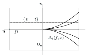
Figure 1. Cerf’s diagram and the setting to construct the carousel.

The geometrical meaning of the carousel is the following: we first take a representative $C$ of the plane curve on some open neighbourhood $W$ of the origin in the plane $\mathbb{C}^{2}$. Let $L$ be the intersection of $W$ with the axis $\{u=0\}$. We consider $W$ with the Whitney stratification given by the strata $W-(C\cup L)$, $C-\{0\}$, $L-\{0\}$ and $\{0\}$ and the function germ $\pi_{2}:(W,0)\to(\mathbb{C},0)$ given by $\pi_{2}(u,v)=v$. The choice of $D$ and $D_{\eta}$ is made so that

$$\pi_{2}:D\times\partial D_{\eta}\to\partial D_{\eta}$$

is a proper stratified submersion with the induced stratification in $D\times\partial D_{\eta}$. By conditions (i), (ii) and (iii) in Lemma 4.1, $\omega$ is a stratified vector field on $D\times\partial D_{\eta}$ which is a lifting of the unit tangent vector field on $\partial D_{\eta}$. Hence, its flow provides a local geometric monodromy $h:D\times\{t\}\to D\times\{t\}$ for some $t\in\partial D_{\eta}$, which preserves the point $(0,t)$ and the finite set $C\cap(D\times\{t\})$. By condition (iv), the only fixed point of $h$ is $(0,t)$.

Now we can give the proof of our main result:

Proof of Theorem 0.2.

Assume that $(X,x)\subset(\mathbb{C}^{N},x)$. We take a privileged polydisc $\Delta$ in $\mathbb{C}^{N}$ at $x$ and a small disc $D_{\eta}$ in $\mathbb{C}$ at $0$ such that the restriction

$$f:X\cap\Delta\cap f^{-1}(\partial D_{\eta})\to\partial D_{\eta}$$

is a proper stratified submersion. We claim that there exists a stratified vector field $\xi$ on $X\cap\Delta\cap f^{-1}(\partial D_{\eta})$ which is a lifting of the unit vector field $\theta$ on $\partial D_{\eta}$ whose flow provides a local geometric monodromy with no fixed points. We prove this by induction on the dimension of $X$ at $x$.

Assume first that $\dim(X,x)=1$. Let $X_{1},\dots,X_{r}$ be the analytic branches of $X$ at $x$. Then $X\cap\Delta\cap f^{-1}(\partial D_{\eta})$ is the disjoint union of all the sets $X_{i}\cap\Delta\cap f^{-1}(\partial D_{\eta})$, $i=1,\dots,r$. Hence, it is enough to show the claim in the case that $X$ is irreducible at $x$. Let $n:\tilde{X}\to X$ be the normalization of $X$ at $x$. Since $f\in\mathfrak{m}_{X,x}^{2}$, we can take an analytic extension $\overline{f}:(\mathbb{C}^{N},x)\to(\mathbb{C},0)$ such that $F\in\mathfrak{m}_{N}^{2}$. After a reparametrization, we can assume that $\tilde{X}$ is an open neighbourhood of $0$ in $\mathbb{C}$, $\left\{0\right\}=n^{-1}(x)$ and $F\circ n(s)=s^{k}$, for some $k\geq 2$. In this case, $\theta$ lifts in a unique way by the map $F\circ n$ and has a local geometric monodromy with no fixed points. But $n$ induces a diffeomorphism on $\tilde{X}-\{0\}$ onto $X-\left\{x\right\}$, so we have also a unique lifting on $X\cap\Delta\cap f^{-1}(\partial D_{\eta})$ whose geometric monodromy has no fixed points.

Now we assume the claim is true when $\dim(X,x)=n$ and prove it in the case that $\dim(X,x)=n+1$. Let $\ell:\mathbb{C}^{N}\to\mathbb{C}$ be a generic linear form and consider the map $\Phi=(\ell,f)$. We have a commutative diagram as follows:

where the vertical arrows are the inclusions and $\pi_{2}$ is the projection onto the second component. Here we choose the polydiscs $\Delta$ and $D\times D_{\eta}$ small enough such that $\Phi$ is a Thom proper map (see Lemma 3.2, Theorem 3.6 and Remark 3.7). The stratification in $D\times\partial D_{\eta}$ is given by the strata $D\times\partial D_{\eta}-(C\cup L)$, $(D\times\partial D_{\eta})\cap C$ and $L$, where $L=\{0\}\times\partial D_{\eta}$ and $C=\Delta_{\ell}(f,x)$ is the Cerf’s diagram.

By induction hypothesis, there exists a stratified vector field $\xi_{1}$ on $X\cap\Delta\cap\ell^{-1}(0)\cap f^{-1}(\partial D_{\eta})$ which is a lifting of $\theta$ and whose geometric monodromy has no fixed points. If $C$ is empty, the claim is obvious by Proposition 1.4, so we can assume that $C$ is not empty.

By the carousel Lemma 4.1, there exists a stratified vector field $\omega$ on $D\times\partial D_{\eta}$ which satisfies the conditions (i), (ii), (iii) and (iv) of the lemma. Since $\omega$ is a lifting of $\theta$, it is globally integrable by Theorem 2.12. Moreover, $\omega$ is not zero along $L$ and $(D\times\partial D_{\eta})\cap C$, so we can use the flow of $\omega$ to construct a weakly controlled tube system $\mathcal{T}^{\prime}$ of $D\times\partial D_{\eta}$ such that $\omega$ is weakly controlled. By Corollary 2.13, $\omega$ lifts to a stratified vector field $\xi$ on $X\cap\Delta\cap\Phi^{-1}(D\times\partial D_{\eta})$ which is globally integrable. Moreover, by using a partition of unity, we can construct $\xi$ in such a way that it coincides with $\xi_{1}$ on $X\cap\Delta\cap\ell^{-1}(0)\cap f^{-1}(\partial D_{\eta})$.

Let $F=X\cap\Delta\cap f^{-1}(t)$, with $t\in\partial D_{\eta}$ and consider the geometric monodromy $h:F\to F$ induced by $\xi$. On one hand, $\xi$ is an extension of $\xi_{1}$, so $h(F\cap\ell^{-1}(0))=F\cap\ell^{-1}(0)$ and $h$ has no fixed points on $F\cap\ell^{-1}(0)$. On the other hand, condition (iv) of Lemma 4.1 implies that $h$ does not have fixed points on $F-\ell^{-1}(0)$ either. This completes the proof.

∎

The proof relied on the hypothesis of $f$ being in $\mathfrak{m}_{X,x}^{2}$, and actually this hypothesis is necessary. Here we give a couple of examples which illustrate this fact.

Example 4.2.

Let $(C,0)$ be the ordinary triple point singularity in $(\mathbb{C}^{3},0)$. This is equal to the union of the three coordinate axis in $\mathbb{C}^{3}$ and the defining equations are given by the $2\times 2$-minors of the matrix

$$M=\left(\begin{array}[]{ccc}x&y&z\\ y&z&x\end{array}\right)$$

This gives to $(C,0)$ a structure of isolated determinantal singularity in the sense of [23]. According also to [23], we can construct a determinantal smoothing of $(C,0)$ by taking the $2\times 2$-minors of $M_{t}=M+tA$, where $A$ is a generic $2\times 3$-matrix with coefficients in $\mathbb{C}$ and $t\in\mathbb{C}$.

In fact, let

$$A=\left(\begin{array}[]{ccc}0&1&0\\ 0&0&0\end{array}\right)$$

and let $(X,0)$ be the surface in $(\mathbb{C}^{3}\times\mathbb{C},0)$ defined as the zero set of the $2\times 2$-minors of $M_{t}$. The projection $f:(X,0)\to(\mathbb{C},0)$, $f(x,y,z,t)=t$ provides a flat deformation whose special fibre is $(C,0)$ and whose generic fibre $F=f^{-1}(t)$, for $t\neq 0$, is a smooth curve. We can see $F$ as a kind of “determinantal Milnor fibre” of $(C,0)$.

It follows from [3, page 279] that $F$ is diffeomorphic to a disk with two holes (as in Figure 2) and that the monodromy $h_{*}:H_{1}(F;\mathbb{Z})\to H_{1}(F;\mathbb{Z})$ is the identity. Since $H_{1}(F;\mathbb{Z})\cong\mathbb{Z}^{2}$, the Lefschetz number is $-1$, and hence any local geometric monodromy must have a fixed point. A simple computation shows that $f\notin\mathfrak{m}_{X,x}^{2}$ in this example.

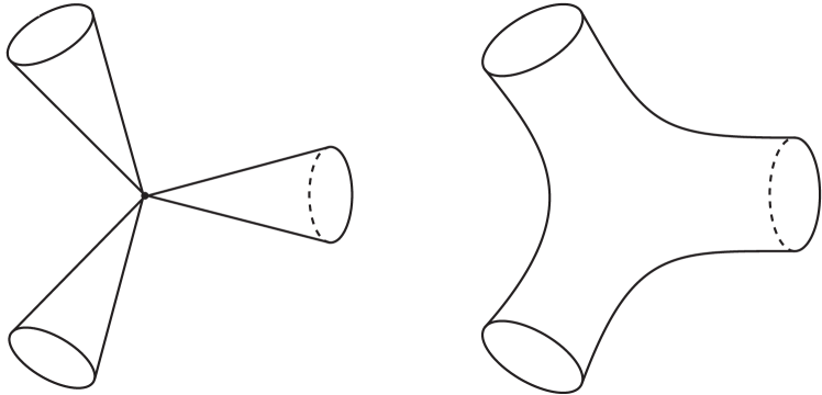
Figure 2. The ordinary triple point singularity and its determinantal Milnor fibre

Example 4.3.

Consider the $A_{4}$ plane curve singularity $(C,0)$ whose equation in $(\mathbb{C}^{2},0)$ is $x^{5}-y^{2}=0$. The monodromy of the classical Milnor fibre of $(C,0)$ is well known and we will not discuss it. Instead, we look at the monodromy of the disentanglement of $(C,0)$ in Mond’s sense (see [21, Chapter 7]). We see $(C,0)$ as the image of the map germ $g_{0}\colon(\mathbb{C},0)\to(\mathbb{C}^{2},0)$ given by $g_{0}(s)=(s^{2},s^{5})$, which has an isolated instability at the origin.

Since we are in the range of Mather’s nice dimensions, we can take a stabilisation, that is, a 1-parameter unfolding $G\colon(\mathbb{C}\times\mathbb{C},0)\to(\mathbb{C}^{2}\times\mathbb{C},0)$, $G(s,t)=(g_{t}(s),t)$ such that for any $t\neq 0$, $g_{t}$ has only stable singularities. By definition, the disentanglement $F$ is the image of the mapping $g_{t}$ intersected with a small enough ball $B$ in $\mathbb{C}^{2}$ centered at the origin and $t$ small enough. Since $F$ is 1-dimensional and connected, it has the homotopy type of a bouquet of spheres (this is true also in higher dimensions by a theorem due to Lê) of dimension 1. The number of such spheres is called the image Milnor number and is denoted by $\mu_{I}(g_{0})$.

Observe that $F$ is also the generic fibre of the function $f:(X,0)\to(\mathbb{C},0)$ where $(X,0)$ is the image of $G$ in $(\mathbb{C}^{2}\times\mathbb{C},0)$ and $f(x,y,t)=t$. We are interested in the local monodromy of $f$ at the origin.

In our case, we take $g_{t}(s)=(s^{2},s^{5}+ts)$. It is easy to see that for $t\neq 0$, $g_{t}$ is an immersion with two transverse double points $p=g_{t}(a_{1})=g_{t}(a_{2})$ and $q=g_{t}(b_{1})=g_{t}(b_{2})$ where $a_{1},a_{2},b_{1},b_{2}$ are the four roots of $s^{4}+t=0$, with $a_{1}=-a_{2}$ and $b_{1}=-b_{2}$. Hence, $g_{t}$ defines a stabilisation of $g_{0}$. Observe that the number of double points coincides with the delta invariant $\delta(C,0)=2$. The disentanglement $F$ is the image of $g_{t}$ and is homeomorphic to the quotient of a closed 2-disk $D_{t}$ under the relations $a_{1}\sim a_{2}$ and $b_{1}\sim b_{2}$ (see Figure 3). Thus, $F$ has the homotopy type of $S^{1}\vee S^{1}$ and $\mu_{I}(g_{0})=2$.

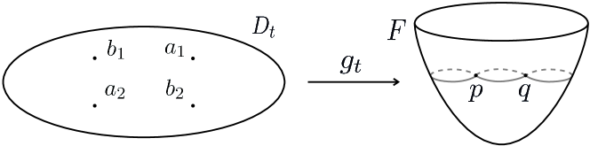
Figure 3. The mapping $g_{t}$ and the double points, $a_{1},b_{1},a_{2}$ and $b_{2}$.

The locally $C^{0}$- trivial fibration is the restriction $f:X\cap(B\times S^{1}_{\eta})\to S^{1}_{\eta}$, for a small enough $\eta>0$.

In order to construct a geometric monodromy $h\colon F\to F$ it is enough to find a 1-parameter group of stratified homeomorphisms $h_{\theta}\colon X\cap(B\times S^{1}_{\eta})\to X\cap(B\times S^{1}_{\eta})$, with $\theta\in\mathbb{R}$, which make commutative the diagram

where $r_{\theta}(t)=e^{i\theta}t$. In this situation, $h:F\to F$ is obtained as the restriction of $h_{2\pi}$.

Since $(C,0)$ is weighted homogeneous with weights $(5,2)$, instead of a Euclidean ball in $\mathbb{C}^{2}$ it is better to consider the (non-Euclidean) ball $B$ given by $|x|^{5}+|y|^{2}\leq 1$. Thus, $C\cap B=g_{0}(D)$, where $D$ is the disk in $\mathbb{C}$ given by $|s|^{10}\leq 1/2$. For $t\neq 0$, $F=g_{t}(D_{t})$, where now $D_{t}=g_{t}^{-1}(B)$ is the disk in $\mathbb{C}$ given by

$$|s|^{10}+|s|^{2}|s^{4}+t|^{2}\leq 1.$$

Given a point $(x,y,t)\in X$, we have $(x,y,t)=G(s,t)$ for some $s\in\mathbb{C}$. We define $h_{\theta}\colon X\to X$ as

$$h_{\theta}(G(s,t))=G\left(e^{\frac{i\theta}{4}}s,e^{i\theta}t\right).$$

We consider in $X$ the stratification given by $\{X-Y,Y\}$, where $Y$ is the double point curve with equations $x^{2}+t=0$, $y=0$. Since $G$ is an embedding on $X-Y$, $h_{\theta}$ is well defined and is a diffeomorphism on $X-Y$. When $(x,y,t)\in Y$ we have $G(s,t)=(s^{2},0,t)$, with $s^{2}=x$ and $s^{4}+t=0$. It follows that

$$h_{\theta}(x,0,t)=G\left(e^{\frac{i\theta}{4}}s,e^{i\theta}t\right)=\left(e^{\frac{i\theta}{2}}s^{2},0,e^{i\theta}t\right)=\left(e^{\frac{i\theta}{2}}x,0,e^{i\theta}t\right),$$

and $\left(e^{i\theta/2}x\right)^{2}+e^{i\theta}t=e^{i\theta}(x^{2}+t)=0$. Thus, $h_{\theta}$ is also well defined on $Y$, $h(Y)=Y$ and the restriction $h\colon Y\to Y$ is a diffeomorphism. It is also clear that $h_{\theta}\colon X\to X$ and its inverse are both continuous, so it is a stratified homeomorphism. It only remains to show that $h_{\theta}(X\cap(B\times S^{1}_{\eta}))=X\cap(B\times S^{1}_{\eta})$, but this a consequence of the equality:

$$\left|e^{\frac{i\theta}{4}}s\right|^{10}+\left|e^{\frac{i\theta}{4}}s\right|^{2}\left|\left(e^{\frac{i\theta}{4}}s\right)^{4}+e^{i\theta}t\right|^{2}=|s|^{10}+|s|^{2}|s^{4}+t|^{2}.$$

The geometric monodromy $h\colon F\to F$ is now the restriction of $h_{2\pi}$, which gives $h(g_{t}(s))=g_{t}\left(e^{i\pi/2}s\right)$, that is, it is obtained by a $\pi/2$-rotation in the disk $D_{t}$.

To finish, we compute $h_{*}\colon H_{1}(F;\mathbb{Z})\to H_{1}(F;\mathbb{Z})$. We recall that $F$ is homeomorphic to the quotient of $D_{t}$ under the relations $a_{1}\sim a_{2}$ and $b_{1}\sim b_{2}$. The four points $a_{1},a_{2},b_{1},b_{2}$ are on a square contained in the interior of $D_{t}$ and centered at the origin, which is obviously invariant under the $\pi/2$-rotation. We denote by $a,b,c,d$ the four edges of the square as in Figure 4.

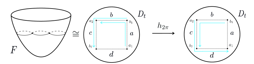
Figure 4. Monodromy of the fiber $F$.

We take the cycles $a+b$ and $c+d$ as a basis of $H_{1}(F;\mathbb{Z})$. Obviously, $h_{*}(a+b)=b+c$ and $h_{*}(b+c)=c+d=-(a+b)$ so the matrix of $h_{*}$ with respect to this basis is:

$$\left(\begin{array}[]{cc}1&0\\ 0&-1\end{array}\right)$$

The Lefschetz number is $1$ and hence, any local geometric monodromy must have a fixed point. In fact, in our construction there is exactly one fixed point, namely, the origin of the disk $D_{t}$ which is invariant under the $\pi/2$-rotation. As in Example 4.2, it is not difficult to check that $f\notin\mathfrak{m}_{X,x}^{2}$.

5. Applications

The first application of Theorem 0.2 is the following corollary, which shows that any hypersurface $(X,x)$ in $\mathbb{C}^{n+1}$ with smooth topological type, must be smooth. We recall that two germs of complex spaces $(X,x)$ and $(Y,y)$ in $\mathbb{C}^{n+1}$ have the same topological type if there exists a homeomorphism $\varphi:(\mathbb{C}^{n+1},x)\to(\mathbb{C}^{n+1},y)$ such that $\varphi(X,x)=(Y,y)$.

Corollary 5.1.

Let $(X,x)$ be a germ of hypersurface in $\mathbb{C}^{n+1}$. If $(X,x)$ has the topological type of a smooth hypersurface, then $(X,x)$ is smooth.

Proof.

If $(X,x)$ has the topological type of a smooth hypersurface then its Milnor fibre is contractible by [13, Proposition, p. 261]. This implies that $(X,x)$ is smooth by [1, Theorem 3]. Observe that Theorem 3 of [1] is a consequence of Theorem 0.2: Let $f:(\mathbb{C}^{n+1},x)\to(\mathbb{C},0)$ be holomorphic which gives a reduced equation of $(X,x)$. The Lefschetz number of the local monodromy of $f$ is 1 and hence, $f\notin\mathfrak{m}_{\mathbb{C}^{n+1},x}^{2}$, by Theorem 0.2. ∎

This corollary is related to Zariski’s multiplicity conjecture [26] which claims that two hypersurfaces in $\mathbb{C}^{n+1}$ with the same topological type have the same multiplicity. Since a hypersurface is smooth if and only if it has multiplicity 1, Corollary 5.1 is just a particular case of the conjecture. Zariski showed the conjecture for plane curves but it remains still open in higher dimensions. Another related result is Mumford’s theorem [22] which states that if $X$ is a normal surface and $X$ is a topological manifold at $x\in X$, then $X$ is smooth at $x$.

Our second application is a no coalescing theorem for families of functions defined on spaces with Milnor property. In [14], the second named author showed the following interesting application of A’Campo’s theorem (see also [5, 12]). Let $\{H_{t}\}_{t\in\mathbb{C}}$ be an analytic family of hypersurfaces defined on some open subset $U\subset\mathbb{C}^{n}$ with only isolated singularities. Take $B$ a Milnor ball for $H_{0}$ around a singular point $x_{0}\in H_{0}$ and assume for all $t$ small enough, the sum of the Milnor numbers of all the singular points of $H_{t}$ in $B$ is constant, that is,

$$\sum_{x\in H_{t}\cap B}\mu(H_{t},x)=\mu(H_{0},x_{0}).$$

Then $H_{t}\cap B$ contains a unique singular point $x$ of $H_{t}$. The purpose of this section is to prove an adapted version of this result in a more general context, namely, for Milnor spaces in the sense of [8]:

Definition 5.2.

A Milnor space is a reduced complex space $X$ such that at each point $x\in X$, the rectified homotopical depth $\operatorname{rhd}(X,x)$ is equal to $\dim(X,x)$.

We refer to [8] for the definition of the rectified homotopical depth and basic properties of Milnor spaces. In general, $\operatorname{rhd}(X,x)\leq\dim(X,x)$, so Milnor spaces are those whose rectified homotopical depth is maximal at any point. Some important properties are the following:

1. any smooth space $X$ is a Milnor space,

2. any Milnor space $X$ is equidimensional,

3. if $X$ is a Milnor space and $Y$ is a hypersurface in $X$ (i.e. $Y$ has codimension one and is defined locally in $X$ by one equation), then $Y$ is also a Milnor space.

As a consequence, any local complete intersection $X$ (not necessarily with isolated singularities) is a Milnor space. Our setting is motivated by the following theorem due to Hamm and Lê (see [8, Theorem 9.5.4]):

Theorem 5.3.

Let $(X,x)$ be a germ of Milnor space and assume that $f\colon(X,x)\to(\mathbb{C},0)$ has isolated critical point in the stratified sense. Then the general fibre $F$ of $f$ has the homotopy type of a bouquet of spheres of dimension $\dim(X,x)-1$.

Corollary 5.4.

With the hypothesis and notation of Theorem 5.3, if $f\in\mathfrak{m}^{2}_{X,x}$, then the trace of the induced map $h_{*}\colon H_{n-1}(F;\mathbb{Z})\to H_{n-1}(F;\mathbb{Z})$ by the monodromy $h:F\to F$ is $(-1)^{n}$, where $n=\dim(X,x)$.

Definition 5.5.

With the hypothesis and notation of Theorem 5.3, the number of spheres of $F$ is called the Milnor number of $f$ and is denoted by $\mu(f)$. We say that the critical point is non-trivial if $\mu(f)>0$.

Let $(X_{0},0)$ be a germ of complex analytic space. Let $f_{0}\colon(X_{0},x_{0})\to(\mathbb{C},0)$ be a germ of holomorphic function. Let $X_{0}$ be a small representative of $(X_{0},0)$ and let ${\mathcal{S}}$ be a Whitney stratification of $X_{0}$. We assume that a representative $f$ has an isolated critical point in the stratified sense at $0$. We define:

Definition 5.6.

A stratified deformation of $(X_{0},x_{0})$ is a flat deformation $\pi\colon({\mathfrak{X}},x_{0})\to(\mathbb{C},0)$, where $\mathfrak{X}$ is an analytic space with an analytic Whitney stratification such that, for a representative $\pi$:

1. $\pi^{-1}(0)=X_{0}$ as analytic spaces,

2. $\pi$ has isolated critical points in the stratified sense,

3. the stratification of $X_{0}$ coincides with the induced stratification by $\mathfrak{X}$ on $\pi^{-1}(0)$.

Given a stratified deformation $\pi\colon({\mathfrak{X}},x_{0})\to(\mathbb{C},0)$, a stratified unfolding is a holomorphic mapping $\mathcal{F}\colon({\mathfrak{X}},x_{0})\to(\mathbb{C}\times\mathbb{C},0)$ such that $p_{1}\circ\mathcal{F}|_{X_{0}}=f_{0}$ and $p_{2}\circ\mathcal{F}=\pi$, where $p_{i}:\mathbb{C}\times\mathbb{C}\to\mathbb{C}$, $i=1,2$, is the $i$th-projection.

We can always assume that $\mathfrak{X}$ is embedded in $\mathbb{C}^{N}\times\mathbb{C}$ and choose coordinates in such a way that $\pi(x,t)=t$. So, we can write the stratified unfolding as $\mathcal{F}(x,t)=(f_{t}(x),t)$. For each $t\in\mathbb{C}$ we have a function $f_{t}\colon X_{t}\to\mathbb{C}$, where $X_{t}=\pi^{-1}(t)$. Here we consider in $X_{t}$ the stratification induced by $\mathfrak{X}$ and denote by $\Sigma(f_{t})$ the set of stratified critical points of $f_{t}$.

Example 5.7.

We consider the function $f_{0}:(X_{0},0)\to(\mathbb{C},0)$, where $X_{0}$ is the surface in $\mathbb{C}^{3}$ given by $z^{2}-y(x^{2}+y)^{2}=0$ and $f_{0}(x,y,z)=x$. The stratification in $X_{0}$ is $\left\{\{0\},C_{0}-\{0\},X_{0}\right\}$, where $C_{0}$ is the curve $z=x^{2}+y=0$. It is easy to see $f_{0}$ has only one critical point in the stratified sense at the origin and that $\mu(f_{0})=1$ (see Figure 5).

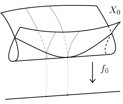
Figure 5. The function $f_{0}$ with a critical point

Now we define a stratified deformation $\pi:(\mathfrak{X},0)\to(\mathbb{C},0)$ and a stratified unfolding $\mathcal{F}\colon({\mathfrak{X}},0)\to(\mathbb{C}\times\mathbb{C},0)$ as follows: $\mathfrak{X}$ is the hypersurface in $\mathbb{C}^{3}\times\mathbb{C}$ with equation $z^{2}-y(x^{2}+y+t)^{2}=0$, $\pi(x,y,z,t)=t$ and $\mathcal{F}(x,y,z,t)=(x,t)$. The stratification in $\mathfrak{X}$ is $\{\{0\},\mathcal{D}-\{0\},\mathcal{C}-\mathcal{D},\mathfrak{X}-\mathcal{C}\}$, where $\mathcal{D}$ is the curve $z=y=x^{2}+t=0$ and $\mathcal{C}$ is the surface $z=x^{2}+y+t=0$. Again it is not difficult to check that all conditions of Definition 5.6 hold.

For $t\neq 0$, $f_{t}:X_{t}\to\mathbb{C}$ has two critical points in the stratified sense at $(\pm\sqrt{-t},0,0)$, which are the points in $D_{t}:=X_{t}\cap\mathcal{D}$. We see that $f_{t}$ has also Milnor number $1$ at each critical point $(\pm\sqrt{-t},0,0)$ (see Figure 6).

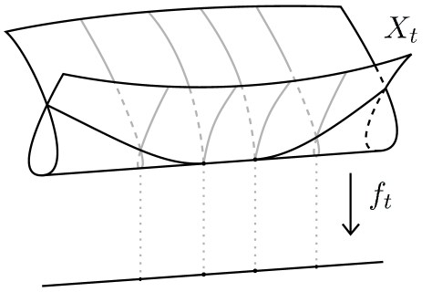
Figure 6. The function $f_{t}$ with two critical points

Theorem 5.8.

Let $f_{0}\colon(X_{0},x_{0})\to(\mathbb{C},0)$ be a function with a non-trivial isolated critical point and let $\mathcal{F}\colon(\mathfrak{X},x_{0})\to(\mathbb{C}\times\mathbb{C},0)$ be a stratified unfolding of $f_{0}$ such that $\mathfrak{X}$ is a Milnor space. We set $Y_{t}=f_{t}^{-1}(0)$ and assume that for any $x\in\Sigma(f_{t})\cap Y_{t}$, the trace of the local monodromy of $f_{t}$ at $x$ in dimension $n-1$ is $(-1)^{n}$, where $\dim(X_{0},x_{0})=n$. Let $B_{0}$ be a Milnor ball for $f_{0}$ at $x_{0}$ and assume that for any $t\in\mathbb{C}$ small enough,

(7) $$\sum_{x\in\Sigma(f_{t})\cap Y_{t}\cap B_{0}}\mu_{x}(f_{t})=\mu_{x_{0}}(f_{0}),$$

where $\mu_{x}(f_{t})$ is the Milnor number of $f_{t}$ at $x$. Then $Y_{t}\cap B_{0}$ contains a unique non-trivial critical point $x$ of $f_{t}$.

Proof.

Denote by $\Sigma(\mathcal{F})$ the set of stratified critical points of $\mathcal{F}$. It follows that $(x,t)\in\Sigma(\mathcal{F})$ if and only if $x\in\Sigma(f_{t})$. Since the stratification of $\mathfrak{X}$ is analytic, $\Sigma(\mathcal{F})$ is also analytic. On one hand,

$$\dim\Sigma(\mathcal{F})\cap\{t=0\}=\dim\Sigma(f_{0})=0$$

and thus, $\dim\Sigma(\mathcal{F})\leq 1$. On the other hand, by (7),

$$\Sigma(\mathcal{F})\cap\{t=t_{0}\}=\Sigma(f_{t_{0}})\neq\emptyset,$$

for $t_{0}\neq 0$, so $\dim\Sigma(\mathcal{F})=1$. Moreover, $\mathcal{F}^{-1}(0)\cap\Sigma(\mathcal{F})=\{0\}$, hence its image $\Delta=\mathcal{F}(\Sigma(\mathcal{F}))$ is also analytic of dimension $1$ in $(\mathbb{C}\times\mathbb{C},0)$ by Remmert’s proper mapping theorem.

We fix a small enough open polydisc $D_{\eta}\times D_{\rho}$ in $\mathbb{C}\times\mathbb{C}$ such that the restriction

(8) $$\mathcal{F}:(B_{0}\times D_{\rho})-\mathcal{F}^{-1}(\Delta)\to(D_{\eta}\times D_{\rho})-\Delta$$

is a proper stratified submersion and such that $\Delta\cap(D_{\eta}\times\{0\})=\{0\}$. By the Thom-Mather first isotopy lemma, (8) is a locally $C^{0}$- trivial fibration. Given $s\in D_{\eta}-\{0\}$, we have $(s,0)\in(D_{\eta}\times D_{\rho})-\Delta$ and hence the fibre,

$$\mathcal{F}^{-1}(s,0)\cap(B_{0}\times D_{\rho})=(f_{0}^{-1}(s)\cap B_{0})\times\{0\},$$

coincides with the general fibre of $f_{0}$.

Let $t\in D_{\rho}$ and assume that $\Sigma(f_{t})\cap f_{t}^{-1}(0)\cap B_{0}=\{x_{1},\dots,x_{k}\}$. For each $i=1,\dots,k$, we take a Milnor ball $B_{i}$ for $f_{t}$ at $x_{i}$ such that $B_{i}$ is contained in the interior of $B_{0}$ and $B_{i}\cap B_{j}=\emptyset$ if $i\neq j$. Now we choose $0<\eta^{\prime}<\eta$ such that for all $s$, with $0<|s|<\eta^{\prime}$, $(s,t)\notin\Delta$.

Fix a point $s\in D_{\eta^{\prime}}$ and consider the loop $\gamma(\theta)=se^{i\theta}$, $\theta\in[0,2\pi]$. This loop induces a monodromy $h:f_{t}^{-1}(s)\cap B_{0}\to f_{t}^{-1}(s)\cap B_{0}$ which coincides, up to isotopy, with the monodromy of $f_{0}$ at $x_{0}$. Moreover, by adding the boundaries of the balls $B_{i}$ as strata in the domain of (8), we can assume that:

1. $h(f_{t}^{-1}(s)\cap B_{i})=f_{t}^{-1}(s)\cap B_{i}$ and $h_{i}=h|_{f_{t}^{-1}(s)\cap B_{i}}$ is the monodromy of $f_{t}$ at $x_{i}$, for each $1=1,\dots,k$;

2. $h$ is the identity outside the interior of $B_{1}\cup\dots\cup B_{k}$.

Let $U=f_{t}^{-1}(s)\cap\left(B_{0}-\cup_{i=1}^{k}\mathring{B}_{i}\right)$ and $V=f_{t}^{-1}(s)\cap\cup_{i=1}^{k}B_{i}$. By considering the Mayer-Vietoris sequence of the pair $(U,V)$ we get a diagram whose rows are exact sequences:

By the exactness in one the rows of the sequence we get

$$a-\left(b+\sum_{i=1}^{k}\mu_{x_{i}}(f_{t})\right)+\mu_{x_{0}}(f_{0})-c+d=0,$$

where $a=\operatorname{rk}H_{n-1}(U\cap V)$, $b=\operatorname{rk}H_{n-1}(U)$, $c=\operatorname{rk}H_{n-2}(U\cap V)$ and $d=\operatorname{rk}H_{n-2}(U)$. Our hypothesis implies that

$$a-b-c+d=0.$$

Now we use the fact that the trace is additive, which gives:

$$a-\left(b+\sum_{i=1}^{k}\operatorname{tr}((h_{i})_{*})\right)+\operatorname{tr}(h_{*})-c+d=0,$$

and hence

$$\sum_{i=1}^{k}\operatorname{tr}((h_{i})_{*})=\operatorname{tr}(h_{*}).$$

Again by hypothesis, $\operatorname{tr}((h_{i})_{*})=\operatorname{tr}(h_{*})=(-1)^{n}$, for all $i=1,\dots,k$, so necessarily $k=1$. ∎

Remark 5.9.

The proof of Theorem 5.8 is just an adaptation of the proof given in [14] for the case $X=\mathbb{C}^{n}$. A similar argument appears also in the paper [4], where it is showed that any family of ICIS with constant total Milnor number has no coalescence of singularities.

References

- [1] Norbert A’Campo. Le nombre de Lefschetz d’une monodromie. Nederl. Akad. Wetensch. Proc. Ser. A 76 = Indag. Math., 35:113–118, 1973.
- [2] Joël Briançon, Philippe Maisonobe, and Michel Merle. Localisation de systèmes différentiels, stratifications de Whitney et condition de Thom. Inventiones Mathematicae, 117(3):531–550, 1994.
- [3] Ragnar-Olaf Buchweitz and Gert-Martin Greuel. The Milnor number and deformations of complex curve singularities. Invent. Math., 58(3):241–281, 1980.
- [4] R. S. Carvalho, J. J. Nuño Ballesteros, B. Oréfice-Okamoto, and J. N. Tomazella. Families of ICIS with constant total Milnor number. Preprint, 2021.
- [5] A. M. Gabrièlov. Bifurcations, Dynkin diagrams and the modality of isolated singularities. Funkcional. Anal. i Priložen., 8(2):7–12, 1974.
- [6] Christopher G. Gibson, Klaus Wirthmüller, Andrew A. du Plessis, and Eduard J. N. Looijenga. Topological stability of smooth mappings. Lecture Notes in Mathematics, Vol. 552. Springer-Verlag, Berlin-New York, 1976.
- [7] Helmut Hamm. Lokale topologische Eigenschaften komplexer Räume. Mathematische Annalen, 191:235–252, 1971.
- [8] Helmut A. Hamm and Lê Dũng Tráng. The Lefschetz Theorem for hyperplane sections. In J. L. Cisneros-Molina, Lê Dũng Tráng, and J. Seade, editors, Handbook of Geometry and Topology of Singularities I, chapter 9. Springer, 2020.
- [9] Helmut A. Hamm and Lê Dũng Tráng. Un théorème de Zariski du type de Lefschetz. Annales Scientifiques de l’École Normale Supérieure. Quatrième Série, 6:317–355, 1973.
- [10] Allen Hatcher. Algebraic topology. Cambridge University Press, Cambridge, 2002.
- [11] Heisuke Hironaka. Stratification and flatness. In Real and complex singularities (Proc. Ninth Nordic Summer School/NAVF Sympos. Math., Oslo, 1976), pages 199–265, 1977.
- [12] Fulvio Lazzeri. A theorem on the monodromy of isolated singularities. In Singularités à Cargèse (Rencontre Singularités Géom. Anal., Inst. Études Sci. de Cargèse, 1972), volume 7 and 8, pages 269–275. Astérisque, 1973.
- [13] Lê Dũng Tráng. Calcul du nombre de cycles évanouissants d’une hypersurface complexe. Ann. Inst. Fourier (Grenoble), 23(4):261–270, 1973.
- [14] Lê Dũng Tráng. Une application d’un théorème d’A’Campo à l’équisingularité. Nederl. Akad. Wetensch. Proc. Ser. A 76=Indag. Math., 35:403–409, 1973.
- [15] Lê Dũng Tráng. La monodromie n’a pas de points fixes. Journal of the Faculty of Science. University of Tokyo. Section IA. Mathematics, 22(3):409–427, 1975.
- [16] Lé Dũng Tráng. Vanishing cycles on complex analytic sets. Sūrikaisekikenkyūsho Kōkyūroku, (266):299–318, 1976.
- [17] Lê Dũng Tráng and Aurélio Menegon Neto. Vanishing polyhedron and collapsing map. Mathematische Zeitschrift, 286(3-4):1003–1040, 2017.
- [18] Lê Dũng Tráng, J. J. Nuño-Ballesteros, and J. Seade. The topology of the Milnor fibration. In J. L. Cisneros-Molina, Lê Dũng Tráng, and J. Seade, editors, Handbook of Geometry and Topology of Singularities I, chapter 6. Springer, 2020.
- [19] John Mather. Notes on topological stability. American Mathematical Society. Bulletin. New Series, 49(4):475–506, 2012.
- [20] John Milnor. Singular points of complex hypersurfaces. Annals of Mathematics Studies, No. 61. Princeton University Press, Princeton, N.J.; University of Tokyo Press, Tokyo, 1968.
- [21] David Mond and J. J. Nuño Ballesteros. Singularities of mappings, volume 357 of Grundlehren der mathematischen Wissenschaften. Springer, Cham, 2020.
- [22] David Mumford. The topology of normal singularities of an algebraic surface and a criterion for simplicity. Inst. Hautes Études Sci. Publ. Math., (9):5–22, 1961.
- [23] J. J. Nuño Ballesteros, B. Oréfice-Okamoto, and J. N. Tomazella. The vanishing Euler characteristic of an isolated determinantal singularity. Israel J. Math., 197(1):475–495, 2013.
- [24] David Prill. Local classification of quotients of complex manifolds by discontinuous groups. Duke Mathematical Journal, 34:375–386, 1967.
- [25] Bernard Teissier. Variétés polaires. II. Multiplicités polaires, sections planes, et conditions de Whitney. In Algebraic geometry (La Rábida, 1981), volume 961 of Lecture Notes in Math., pages 314–491. Springer, Berlin, 1982.
- [26] Oscar Zariski. Some open questions in the theory of singularities. Bull. Amer. Math. Soc., 77:481–491, 1971.