The stellar mass in and around isolated central galaxies: connections to the total mass distribution through galaxy-galaxy lensing in the Hyper Suprime-Cam survey

Abstract

Using photometrically selected galaxies from the Hyper Suprime-Cam (HSC) imaging survey, we measure the stellar mass density profiles for satellite galaxies as a function of the projected distance, $r_{p}$, to isolated central galaxies (ICGs) selected from SDSS/DR7 spectroscopic galaxies at $z\sim 0.1$. By stacking HSC images, we also measure the projected stellar mass density profiles for ICGs and their stellar halos. The total mass distributions are further measured from HSC weak lensing signals. ICGs dominate within $\sim$0.15 times the halo virial radius ($0.15R_{200}$). The stellar mass versus total mass fractions drop with the increase in $r_{p}$ up to $\sim 0.15R_{200}$, beyond which the fractions are less than 1% while stay almost constant, indicating the radial distribution of satellites trace dark matter. The integrated stellar mass locked in satellites is proportional to the virial mass of the host halo, $M_{200}$, for ICGs more massive than $10^{10.5}\mathrm{M}_{\odot}$, i.e., $M_{\ast,\mathrm{sat}}\propto M_{200}$, whereas the scaling relation between the stellar mass of ICGs $+$ stellar halos and $M_{200}$ is close to $M_{\ast,\mathrm{ICG+diffuse}}\propto M_{200}^{1/2}$. Below $10^{10.5}\mathrm{M}_{\odot}$, the change in $M_{200}$ is much slower with the decrease in $M_{\ast,\mathrm{ICG+diffuse}}$. At fixed stellar mass, red ICGs are hosted by more massive dark matter halos and have more satellites. Interestingly, at $M_{200}\sim 10^{12.7}\mathrm{M}_{\odot}$, both $M_{\ast,\mathrm{sat}}$ and the fraction of stellar mass in satellites versus total stellar mass, $f_{\mathrm{sat}}$, tend to be marginally higher around blue ICGs, perhaps implying the late formation of blue galaxies. $f_{\mathrm{sat}}$ increases with the increase in both $M_{\ast,\mathrm{ICG+diffuse}}$ and $M_{200}$, and scales more linearly with $M_{200}$. We provide best-fitting relations to $M_{200}$ versus $M_{\ast,\mathrm{ICG+diffuse}}$, $M_{\ast,\mathrm{sat}}$ or $M_{\ast,\mathrm{ICG+diffuse}}+M_{\ast,\mathrm{sat}}$, and to $f_{\mathrm{sat}}$ versus $M_{200}$ or $M_{\ast,\mathrm{ICG+diffuse}}$, for red and blue ICGs separately.

1 Introduction

In the structure formation paradigm of $\Lambda$CDM, galaxies form by the cooling and condensation of gas at centers of dark matter halos (White & Rees, 1978). It is usually believed that galaxy formation involves two phases, an early rapid formation of “in-situ” stars through gas cooling and a later phase of mass growth through accretion of smaller satellite galaxies, which were originally central galaxies of smaller dark matter halos. These smaller halos and galaxies, after falling into larger halos, become the so-called subhalos and satellite galaxies. These satellites lose their stellar mass due to tidal stripping. Stripped stellar materials typically lie in the outskirts of central galaxies and are more metal poor than “in-situ” stars, which form the diffuse light or the extended stellar halos around the central galaxies (e.g. Bullock & Johnston, 2005; Cooper et al., 2010).

Many observational studies on satellite galaxies and the faint diffuse stellar halos focused on the Local Group (LG) or the very nearby Universe because of the greater depth and detail with which nearby galaxies can be studied. Particular concerns have been paid to comparing $\mathrm{\Lambda}\text{CDM}$ predictions to the abundance and internal structure of dwarf spheroidal galaxies in and around the LG (e.g. Klypin et al., 1999; Moore et al., 1999; Koposov et al., 2009; Font et al., 2011; Tollerud et al., 2011; Boylan-Kolchin et al., 2011) and to the low surface brightness stellar halos of disc galaxies similar to our Milky Way (MW) Galaxy (e.g. Merritt et al., 2016; Harmsen et al., 2017; Merritt et al., 2020; Keller, 2021). Such studies are limited by the fact that the nearby Universe contains limited number of galaxies, as considerable scatter is expected among systems of similar mass halos (e.g. Guo et al., 2015; Cautun et al., 2015a; Carlsten et al., 2021; Mao et al., 2021).

Early studies of extra-galactic satellites in the more distant Universe often rely on spectroscopic surveys with redshift information to study their projected number density profiles to the central galaxies(e.g. Vader & Sandage, 1991; Sales & Lambas, 2005; Chen et al., 2006). Spectroscopic redshifts enable the direct discrimination between true satellites and background sources. However, satellites with redshift information are usually about only one to two magnitudes fainter than the central galaxy in most existing wide field spectroscopic surveys. To study smaller and fainter satellites, quite a few studies attempted to combine a redshift survey (for centrals) with a photometric survey (for satellites), which can reach several magnitudes fainter than pure spectroscopic surveys. Results can be achieved by stacking satellite counts around a large sample of central galaxies (e.g. Phillipps & Shanks, 1987; Lorrimer et al., 1994; Wang et al., 2011; Lares et al., 2011; Wang & White, 2012; Guo et al., 2012; Tal et al., 2012; Jiang et al., 2012; Nierenberg et al., 2013; Wang et al., 2014; Cautun et al., 2015b; Lan et al., 2016). Stacking not only helps to increase the signal-to-noise level, but also the foreground and background source contamination can be subtracted statistically.

Similarly, studies on low surface brightness stellar halos of distant extra-galactic systems often rely on stacking images of a large sample of galaxies with similar properties (e.g. Zibetti et al., 2004, 2005; Tal & van Dokkum, 2011; D’Souza et al., 2014; Wang et al., 2019; Zhang et al., 2019). This is because the surface brightness, $I$, of extended objects drops with distance, in a relationship with redshift, $z$, as $I\propto(1+z)^{-4}$. Hence for more distant galaxies, the surface brightness of their faint stellar halos can be only a few percent or even less than the sky background. This makes it more difficult to study distant stellar halos individually. Fortunately, the noise level of the stacked image can be significantly decreased with the increase in the number of input images used for stacking. It enables the detection of the averaged signals for extended stellar halos, which were once below the noise level of individual images.

The observed abundance and properties of satellite galaxies, the total mass or emission in central galaxies and their diffuse stellar halos, and their connections to the host dark matter halos are important aspects to qualitatively test the theory of galaxy formation. It has been recognized that more massive central galaxies have higher abundance of satellites and more dominant outer stellar halos (e.g. Wang et al., 2011; Guo et al., 2011a; Jiang et al., 2012; Wang et al., 2014; D’Souza et al., 2014; Lan et al., 2016). In addition, there are more satellites and also more extended stellar halos around red passive centrals than blue centrals with the same stellar mass (e.g. Peng et al., 2012; Wang & White, 2012; D’Souza et al., 2014). So far, observations are generally consistent with predictions by theoretical studies (e.g. Purcell et al., 2007; Oser et al., 2010; Lackner et al., 2012; Pillepich et al., 2014; Rodriguez-Gomez et al., 2016; Karademir et al., 2018; Cooper et al., 2013; Kawinwanichakij et al., 2014; Cooper et al., 2015; Rodriguez-Gomez et al., 2016).

The halo mass versus stellar mass relation of central galaxies have been investigated in many previous studies, based on a few different approaches including abundance matching (e.g. Guo et al., 2010), Halo Occupation Distribution modelling (e.g. Wang & Jing, 2010; Moster et al., 2010, 2013; Wang et al., 2013b, a) or lensing measurements (e.g. Leauthaud et al., 2012; Hudson et al., 2015; Han et al., 2015a). It has been generally recognized that the relation shows a transition around MW mass, above which halo mass changes more rapidly with stellar mass and below which halo mass changes very slowly with the decrease in stellar mass. However, many existing studies did not distinguish central galaxies by color upon determining the relations. In addition, the emissions in the outer stellar halos of massive elliptical galaxies are often failed to be detected in shallow surveys such as SDSS, resulting in under estimates in the total luminosity or stellar mass of central galaxies (e.g. He et al., 2013; D’Souza et al., 2015).

Alternatively, many studies use satellite abundance as a proxy to the host halo mass (e.g. Peng et al., 2012; Wang & White, 2012; Sales et al., 2013; Rodríguez-Puebla et al., 2015; Man et al., 2019). Indeed, as have been proved by weak lensing measurements, red passive centrals not only have more satellites, but also they are hosted by more massive dark matter halos than blue centrals with the same stellar mass (Mandelbaum et al., 2016), indicating a tight relation between satellite abundance and host halo mass. Recently, Tinker et al. (2019) further suggested that the total luminosity of satellites brighter than a certain magnitude threshold can be used as a good proxy to the host halo mass.

In this paper, we at first re-investigate the role of satellites as proxies to their host halo mass, by counting and averaging photometric companions from the Hyper Suprime-Cam (HSC) deep imaging survey around spectroscopically identified isolated central galaxies selected from SDSS/DR7. We avoid the small scale regions close to the central galaxies, which are significantly affected by source deblending mistakes. We calculate the average projected stellar mass density profiles for satellites, and for red and blue central galaxies separately. The integrated stellar mass in these satellites will be directly compared with the best-constrained host halo mass through weak lensing signals.

In addition to satellites, the projected stellar mass density profiles for central galaxies and their stellar halos will be measured and investigated in this paper as well, and for red and blue centrals separately. Based on the HSC imaging data products, Wang et al. (2019) (hereafter Paper I) have measured the PSF-corrected surface brightness profiles by stacking images of isolated central galaxies. In this study we follow the approach in Paper I but further convert the surface brightness profiles to projected stellar mass density profiles. The integrated stellar mass over the profile after stacking include the contribution from the faint outer stellar halos, which was not fully detectable in shallow surveys or before stacking.

Combining the measurements of satellites, centrals and their stellar halos, we are able to investigate the radial distribution of total stellar mass versus dark matter. We also investigate the connection between satellites and central galaxies $+$ their diffuse stellar halos, including the fraction of stellar mass in satellites versus the total stellar mass, and the transition radius beyond which satellites dominate. This is the first attempt of measuring the projected stellar mass density profiles for both the diffuse stellar halos and satellite galaxies in the same paper.

We introduce our sample selection of halo central galaxies, the HSC photometric source catalog and imaging products, and the HSC shear catalog in Section 2. Our method of satellite counting and stacking, image stacking, PSF and $K$-corrections and lensing measurements are detailed in Section 3. Results are presented in Section 4. We conclude in the end (Section 5).

We adopt as our fiducial cosmological model the first-year Planck cosmology (Planck Collaboration et al., 2014), with values of the Hubble constant $H_{0}=67.3\mathrm{kms^{-1}/Mpc}$, the matter density $\Omega_{m}=0.315$ and the cosmological constant $\Omega_{\Lambda}=0.685$.

2 data

2.1 Isolated central galaxies

To identify a sample of galaxies with a high fraction of central galaxies in dark matter halos (purity), we select galaxies that are the brightest within given projected and line-of-sight distances. The parent sample used for this selection is the NYU Value Added Galaxy Catalog (NYU-VAGC; Blanton et al., 2005), which is based on the spectroscopic Main galaxy sample from the seventh data release of the Sloan Digital Sky Survey (SDSS/DR7; Abazajian et al., 2009). The sample includes galaxies in the redshift range of $z=0.001$ to $z\sim 0.4$, which is flux limited down to an apparent magnitude of 17.77 in SDSS $r$-band, with most of the objects below redshift $z=0.25$.

Following D’Souza et al. (2014), we at first exclude galaxies whose minor to major axis ratios are smaller than 0.3, which are likely edge-on disc galaxies. de Jong (2008) pointed out that the scattered light through the far wings of point spread function (PSF) from edge-on disc galaxies can significantly contaminate the signal of stellar halos.

We require that galaxies are the brightest within the projected virial radius, $R_{200,\mathrm{AM}}$, of their host dark matter halos and within three times the virial velocity along the line-of-sight direction. Moreover, these galaxies should not be within the projected virial radius (also three times virial velocity along the line-of-sight) of another brighter galaxy. The virial radius and velocity are derived through the abundance matching formula of Guo et al. (2010), and thus we use the index AM here to denote abundance matching. It has been demonstrated that the choice of three times virial velocity along the line-of-sight is a safe criterion that identifies all true companion galaxies (Sales et al., 2013).

The SDSS spectroscopic galaxies suffer from the fiber collision effect that two fibers cannot be placed closer than 55$\arcsec$. To avoid the case when a galaxy has a brighter companion but this companion is not included in the SDSS spectroscopic sample, we use the SDSS photometric catalog to make further selections. The photometric catalog is the value-added Photoz2 catalog (Cunha et al., 2009) based on SDSS/DR7, which provides photometric redshift probability distributions for SDSS galaxies. We further discard galaxies that have a photometric companion, whose redshift is not available but is within the projected separation of the given selection criterion, and its photoz probability distribution gives a larger than 10% of probability that it shares the same redshift as the central galaxy.

We provide in the third to fifth columns of Table LABEL:tbl:icg the numbers of all, red and blue isolated central galaxies. The color division is slightly stellar mass dependent (see Wang & White (2012) for details). The total number of galaxies in each bin is larger than that in Paper I. This is because in Paper I we did not perform $K$-corrections, which accounts for the band shift due to cosmic expansion, and thus a narrower redshift range of $0.05<z<0.16$ was adopted to reduce the effect introduced by ignoring $K$-corrections. In this paper, we include $K$-corrections, and thus all ICGs over a wider redshift range are used. In Paper I, we investigated the purity and completeness of isolated central galaxies by using the mock galaxy catalog built from the Munich semi-analytical model of galaxy formation (Guo et al., 2011b). We found galaxies selected in this way have more than 85% of being true halo central galaxies, and the completeness is above 90%. Hereafter, we call our sample of isolated central galaxies in short as ICGs.

2.2 HSC imaging data and photometric sources

Table 1: Average halo virial radius ($R_{200,\mathrm{mock}}$) and number ($N$) of all, red and blue isolated central galaxies in six stellar mass bins considered in this study. $R_{200,\mathrm{mock}}$ is based on isolated central galaxies in a mock galaxy catalog built from the Munich semi-analytical model of galaxy formation (Guo et al., 2011b), rather than using abundance matching.

$\log M_{*}/\mathrm{M}_{\odot}$	$R_{200,\mathrm{mock}}$ [kpc]	$N_{\mathrm{galaxy}}$	$N_{\mathrm{red}}$	$N_{\mathrm{blue}}$
11.4-11.7	758.0	1008	964	44
11.1-11.4	459.08	3576	3026	550
10.8-11.1	288.16	6370	4345	2023
10.5-10.8	214.80	6008	3142	2861
10.2-10.5	173.18	3771	1353	2418
9.9-10.2	121.1	3677	700	2977

HSC-SSP (Aihara et al., 2018a) is based on the new prime-focus camera, the Hyper Suprime-Cam (Miyazaki et al., 2012, 2018; Komiyama et al., 2018; Furusawa et al., 2018) on the 8.2-m Subaru telescope. It aims for a wide field of 1,400 deg² with a depth of $r\sim 26$, a deep field of 26 deg² with a depth of $r\sim 27$ and an ultra-deep field of 3.5 deg² with one magnitude fainter. In this paper we focus on the wide field data. HSC photometry covers five bands (HSC-$grizy$). The transmission curves and wavelength ranges for HSC $gri$-bands are almost the same as those of SDSS (Kawanomoto et al., 2018).

HSC-SSP data is processed using the HSC pipeline, which is a specialized version of the LSST (Axelrod et al., 2010; Jurić et al., 2017) pipeline code. Details about the HSC pipeline are available in the pipeline paper (Bosch et al., 2018), and here we only introduce the main data reduction steps and the corresponding data products of HSC.

In the context of HSC, a single exposure is called one “visit” with a unique “visit” number. The same sky field is “visited” multiple times. The HSC pipeline involves four main steps: (1) processing of single exposure (one visit) image (2) joint astrometric and photometric calibration (3) image coaddition and (4) coadd measurement.

In the first step, bias, flat field and dark flow are corrected for. Bad pixels, pixels hit by cosmic rays and saturated pixels are masked and interpolated. The pipeline first performs an initial background subtraction before source detection. Detected sources are matched to external reference catalogs in order to calibrate the zero point and a gnomonic world coordinate system for each CCD. After galaxies and blended objects are filtered out, the sky background is estimated and subtracted again, based on blank pixels that do not contain any detection. A secure sample of stars are used to construct the central PSF model. The outputs of this step are called Calexp images (means “calibrated exposure”). They are given on individual exposure basis.

In the second joint calibration step, the astrometric and photometric calibrations are refined by requiring that the same source appearing on different locations of the focal plane during different visits should give consistent positions and fluxes. Readers can find details in Bosch et al. (2018). The joint calibration improves the accuracy of both astrometry and photometry.

In the third step, the HSC pipeline resamples images to the pre-defined output skymap. It involves resampling both the single exposure images and the PSF model (Jee & Tyson, 2011) using a 3rd (for internal releases earlier than and also including S18a) or 5th-order (For S19a and later releases) Lanczos kernel. Resampled images of different visits are then combined together (coaddition). Images produced through coaddition are called coadd images.

In the last step, objects are detected, deblended and measured from the coadd images. A maximum-likelihood detection algorithm is run independently for each band. Background is estimated and subtracted once again. The detected footprints and peaks of sources are merged across different bands to maintain detections that are consistent over different bands and to remove spurious peaks. These detected peaks are deblended and a full suite of source measurement algorithm is run on all objects, yielding independent measurements of source positions and other properties in each band. A reference band of detection is then defined for each object based on both the signal-to-noise ratio (SNR) and the purpose of maximizing the number of objects in the reference band. Finally, the measurement of sources are run again with the position and shape parameters fixed to the values in the reference band to achieve the “forced” measurement. The forced measurement brings consistency across bands and enables computing object colors using the magnitude difference in different bands.

The faint stellar halo to be studied in this paper can be less than a few percent of the sky background, and thus it is crucial to properly model and subtract the sky background. The HSC internal data releases S15, S16 and S17 used a 6th-order Chebyshev polynomial to fit individual CCD images to model the local sky background and instrumental features. It over-subtracts the light around bright sources and leaves a dark ring structure around bright galaxies. The over-subtraction is mainly caused by the scale of the background model (or order of the polynomial fitting) and unmasked outskirts of bright objects. It is difficult to know how extended objects are before coaddition.

The internal S18a data release implements a significantly improved global background subtraction approach (Aihara et al., 2019). An empirical background model crossing all CCDs are used to model the sky background, meaning that discontinuities at CCD edges are avoided. A scaled “frame”, which is the mean response of the instrument to the sky for a particular filter, is used to correct for static instrumental features that have a smaller scale than the empirical background model. As have been shown in Aihara et al. (2019) and Wang et al. (2019), artificial instrumental features over the focal plane have been successfully removed following the use of the S18a data, leaving uniform image backgrounds. The S18a release also adopts a larger scale of about 1000 pixels to model the sky background, which minimizes the problem of oversubtraction.

While the global background subtraction approach has helped to avoid over-subtracting the extended outskirts of galaxies, it introduces new issues due to sky background residuals. One notable issue is that cModel fluxes are over-estimated for some of the faint sources, and occasionally even a fake detection has a large flux. Thus for the S19a data release, the pipeline performs the global background subtraction as S18a when processing single exposures, but it enables a local background subtraction upon coadd image processing for detailed measurements (e.g., galaxy shape and photometric redshift estimations). The issues due to sky background residuals have been mitigated in S19a though not completely eliminated.

In our analysis throughout the main text of this paper, we use coadd images of the S18a internal data release to stack galaxy images and calculate the projected stellar mass density profiles of central galaxies and their stellar halos. In addition, we use primary photometric sources which are classified as extended from the S19a internal data release to calculate the radial distribution of satellite galaxies. We exclude sources with any of the following flags set as true in $g$, $r$ and $i$-bands: bad, crcenter, saturated, edge, interpolatedcenter or suspectcenter. The S19a bright star masks are created based on stars from Gaia DR2, and we have excluded sources within the ghost, halo and blooming masks of bright stars in $i$-band. We also limit to footprints reaching full depth in $g$ and $r$-bands. As have been discussed by Aihara et al. (2018b) and Wang et al. (2021), the completeness of photometric sources in HSC is very close to 1 at $r\sim 25$, and thus we adopt a flux limit of $r<25$. The total area is a bit more than 450 square degrees.

2.3 HSC shear catalog

We use the HSC second-year shape catalog (Li et al., in prep.) produced from the $i$-band wide field of HSC S19a internal data release (Aihara et al., in prep.). The catalog covers an area of $433.48~{}\rm{deg}^{2}$ with a mean seeing of $0.59\arcsec$. With conservative galaxy selection criteria, the raw galaxy source number density are $22.94/\rm{arcmin}^{2}$.

The shapes of galaxies are estimated with the re-Gaussianization PSF correction method (Hirata & Seljak, 2003). The output of the re-Gaussianization estimator is the galaxy ellipticity:

$$(e_{1},e_{2})=\frac{1-(b/a)^{2}}{1+(b/a)^{2}}(\cos 2\phi,\sin 2\phi),$$ (1)

where $b/a$ is the axis ratio, and $\phi$ is the position angle of the major axis with respect to the equatorial coordinate system.

The shapes are calibrated with realistic image simulations downgrading the galaxy images from Hubble Space Telescope (Koekemoer et al., 2007) to the HSC galaxy images (Mandelbaum et al., 2018a). The calibration removes the galaxy property-dependent (galaxy resolution, galaxy SNR, and galaxy redshift) shear estimation bias (i.e., multiplicative bias and additive bias). The multiplicative bias and additive bias for a galaxy ensemble are:

$$\begin{split}\hat{m}&=\frac{\sum_{i}w_{i}m_{i}}{\sum_{i}w_{i}},\\ \hat{c}_{1,2}&=\frac{\sum_{i}w_{i}a_{i}e^{\rm{PSF}}_{1,2;i}}{\sum_{i}w_{i}},\end{split}$$ (2)

respectively. Here, $i$ refers to the galaxy index. $w_{i}$, $m_{i}$ and $a_{i}$ are the galaxy shape weight, multiplicative bias and fractional additive bias for galaxy $i$. The galaxy shape weight is defined as

$$w=\frac{1}{\sigma_{e}^{2}+e_{\rm{rms}}^{2}},$$ (3)

where $e_{\rm{rms}}$ is the root-mean-square (RMS) of intrinsic ellipticity per component, and $\sigma_{e}$ refers to the shape measurement error per component due to photon noise. $e_{\rm{rms}}$ and $\sigma_{e}$ are modeled and estimated for each galaxy using the image simulation. The calibrated shear estimation for the galaxy ensemble is:

$$\hat{g}_{1,2}=\frac{\sum_{i}w_{i}e_{1,2;i}}{2\mathcal{R}(1+\hat{m})\sum_{i}w_{i}}-\frac{\hat{c}_{1,2}}{1+\hat{m}}.$$ (4)

Here $\mathcal{R}$ is the shear responsivity, defined as the response of the ensemble averaged ellipticity to a small shear (Bernstein & Jarvis, 2002).

3 Method

In the following, we introduce in Sec. 3.1 the satellite counting and background subtraction methodologies. To calculate the stellar mass distribution of ICGs and their diffuse stellar halos, we at first stack galaxy images to obtain the PSF-corrected surface brightness profiles (Section 3.2). $K$-corrections are then achieved for each individual galaxy (Section 3.3). In the end, the surface brightness profiles are converted to the projected stellar mass density profiles based on the $K$-corrected and PSF free color profiles (Section 3.4). We introduce how the differential total mass density profiles are calculated from weak lensing signals in Section 3.5.

3.1 Satellite counts and background subtraction

To calculate the projected density profiles of stellar mass in resolved satellites around ICGs, we make use of the HSC source catalog, which is flux limited down to the $r$-band apparent magnitude of $r\sim 25$.

We follow the method of Wang & White (2012) and Wang et al. (2014) to make satellite counts. Around each ICG, we count all companions in projected radial bins, with the projected distances to ICGs computed from the angular separation and the redshift of the ICG. This includes both true satellites and fore/background contaminations. For each companion, the $K$-correction formula of Westra et al. (2010) is applied by using its apparent color and also assuming it is at the same redshift as the ICG. Further after distance modulus correction using the redshift of the central ICG, we obtain absolute magnitudes and rest-frame colors. A conservative red end cut of ${}^{0.1}(g-r)<0.065\log_{10}M_{\ast}/\mathrm{M}_{\odot}+0.35$ is then made to the rest-frame colors of companions to eliminate the population of background sources which are too red to be at the same redshifts of ICGs, and hence increase the signal. To estimate the stellar-mass-to-light ratios, we adopt a Gaussian Process Regression (GPR) fitting procedure, which estimates the stellar mass of each companion through its color and will be introduced in detail in Sec. 3.4.

Weighting companion number counts in different radial bins by their stellar mass, we obtain their projected stellar mass density profiles around each ICG, which are based on companions with $\log_{10}M_{\ast,\mathrm{ICG}}-3<\log_{10}M_{\ast,\mathrm{sat}}<\log_{10}M_{\ast,\mathrm{ICG}}$. To ensure the completeness of satellites given the HSC flux limit of $r<25$, we allow a particular central ICG to contribute counts only if the stellar mass corresponding to $r=25$ at the redshift of the ICG and lying on the red envelope of the intrinsic color distribution is smaller than $\log_{10}M_{\ast,\mathrm{ICG}}-3$. Counts around all ICGs in the same stellar mass bin are cumulated and averaged to give the final profiles.

To subtract fore/background sources, we repeat exactly the same steps with a sample of random points, which are assigned the same redshift and stellar mass distributions as ICGs. Centered on these random points, we calculate a suite of random profiles. The random profiles are subtracted from the profiles centered on real ICGs, to obtain the projected stellar mass density profiles of real satellite galaxies.

Throughout the analysis of this paper, we consider the radial range, which is within 0.1 times the halo virial radius, $0.1R_{200}$, as have been significantly affected by source deblending issues. We provide details about how this inner radius cut is determined in Appendix A. In the following sections, results over the entire radial range will still be presented, but the measured profiles of satellite galaxies within $0.1R_{200}$ should be avoided for any scientific inferences.

3.2 Surface brightness profiles of ICGs and stellar halos

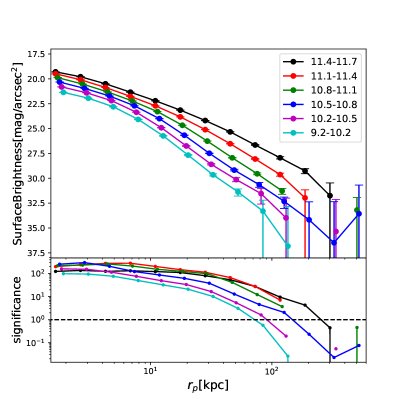
Figure 1: Upper panel: Averaged surface brightness profiles for ICGs $+$ their stellar halos. ICGs are grouped into a few stellar mass bins, as indicated by the legend in log stellar mass. All ICGs in the redshift range of $0.01<z<0.3$ are used. No $K$-correction or PSF-correction have been applied. Errorbars are 1-$\sigma$ scatters of 100 boot-strapped subsamples. Lower panel: Measured surface brightness profiles divided by their 1-$\sigma$ errors.

The readers can find details about how we process galaxy images and calculate the surface brightness profiles of ICGs and their outer stellar halos in Paper I. In this subsection, we introduce our main steps.

Centered on each ICG, we extract its image cutout with edge length of $2\times 1.3$ times the virial radius, $R_{200,\mathrm{mock}}$. Here the values of $R_{200,\mathrm{mock}}$ for ICGs in a few different ranges of stellar mass are provided in the second column of Table LABEL:tbl:icg, which are estimated from ICGs in the mock galaxy catalog of Guo et al. (2011b). The physical scales are converted to angular sizes according to the redshifts of the ICGs. Each image cutout is divided by the zero point flux. Bad pixels such as those which are saturated, close to CCD edges, outside the footprint with available data, hit by cosmic rays and so on, are masked. We correct the effect of "cosmic dimming" by multiplying the image cutout of each ICG by $(1+z)^{4}$. The cutouts are resampled to ensure the same number of pixels within $R_{200,\mathrm{mock}}$. Each pixel has a fixed physical scale of 0.8 kpc.

To look at the ICGs and their diffuse stellar halos, all other companion sources, including physically associated satellites and fore/background sources, are detected and masked. Here we choose a combination of 0.5, 1.5, 2 and 3 times the background noise levels as detection thresholds and successively apply them to the image cutouts. Note when adopting 0.5 times the background noise as the threshold, we only use footprints which are also associated with sources detected by 1.5 times the background noise level as well. This is to avoid faked detections below the noise level. The readers can check Paper I for more detailed comparisons on different choices of source detection and masking thresholds.

We stack images for ICGs with similar properties (e.g. in the same stellar mass bin of Table LABEL:tbl:icg and/or having similar colors). Stacking helps us to go beyond the noise level of individual images. For each pixel in the output image plane, we at first clip corresponding pixels from all input images (masked pixels are not included) by discarding 10% pixels near the two ends of the distribution tail. We have checked that varying this fraction between 1% and 10% does not bias the stacked surface brightness profiles.

In the end, to account for any residual sky background, we repeat the same steps for image cutouts centered on a sample of random points within the HSC footprint, and the random stacks are subtracted from the stacks of real galaxies. These random points are assigned the same redshift and stellar mass distributions as real galaxies. As have been shown in Paper I, the random stacks look ideally uniform and show flat surface brightness profiles which agree very well with the large-scale surface brightness profiles centered on real galaxies. In addition, the random stacks can account for incomplete masking of fore/background companion sources.

Many previous studies tried to align galaxy images along their major axis before stacking and calculate the surface brightness profiles based on elliptical isophotal contours, which are reported as functions of the semi-major axis lengths. In our analysis, we choose not to rotate galaxy images. So basically our stacked images are circularly averaged. As we have discussed in Paper I, because we have excluded extremely edge-on galaxies, circularly averaged profiles show only slightly steeper color profiles than major-axis aligned and elliptically averaged profiles if the color gradient is negative, and the surface brightness profiles are not significantly affected.

The averaged 1-dimensional surface brightness profiles can be obtained from stacked images, which are shown by Figure 1 for ICGs in a few different stellar mass bins. Slightly better signals are obtained thanks to the larger sample size than Paper I, especially for the most and least massive stellar mass bins. In addition to the final stacked images and surface brightness profiles, the image cutouts and profiles of individual ICGs processed in this step are saved as well.

After achieving measurements for the 1-dimensional surface brightness profiles, PSF-corrections are made to the profiles in HSC $g$, $r$ and $i$-bands. The corrections are made according to the extended PSF wings measured in Paper I and by fitting PSF-convolved model profiles to the measured surface brightness profiles, in order to estimate the PSF-contamination fraction as a function of projected distance to the center of galaxies. The details are provided in Appendix B. Explicitly, the fraction increases with the increase in projected distance and decrease in stellar mass of ICGs. Interestingly, the fraction is higher around blue late-type galaxies than red early-type galaxies with the same stellar mass. This is mainly because blue galaxies are more extended, and their outer stellar halos are fainter. As a result, PSF tends to scatter more light from the central parts of galaxies to contaminate the signals of the true outer stellar halos.

3.3 $K$-corrections

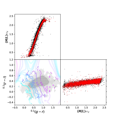
Figure 2: Gaussian Process Regression (GPR) is adopted to recover the $r$-band stellar-mass-to-light ratios ($M_{\ast}/L_{r}$) of SDSS spectroscopic Main galaxies from their ${}^{0.1}(g-r)$ and ${}^{0.1}(r-i)$ colors. The black dots are original values of a randomly picked up 10% subsample used for testing and validation, in which $M_{\ast}/L_{r}$ was estimated from the $K$-corrected colors by fitting a stellar population synthesis model (Blanton & Roweis, 2007) assuming a Chabrier (2003) initial mass function to the SDSS photometry. Red dots are recovered $M_{\ast}/L_{r}$ through GPR. Grey shaded region in the bottom left panel demonstrate the number density distributions of SDSS Main galaxies, while colored contours show the recovered $M_{\ast}/L_{r}$ through GPR.

After achieving PSF corrections for individual ICGs in $g$, $r$ and $i$ filters, we conduct $K$-corrections using the PSF-free color profiles and the redshift of each individual ICG. The empirical $K$-correction formula provided by Westra et al. (2010) is adopted for the correction. Note the individual color profiles can be noisy, and when estimates of the color is not available due to negative flux, we do linear interpolations to obtain the color from neighboring radial bins with non-negative flux values. After including $K$-corrections, we calculate the rest-frame color and surface brightness profile for each individual ICG and its stellar halo, in $g$, $r$ and $i$-bands.

To test the robustness of $K$-corrections, Figure 17 in Appendix D shows the $g-r$ color profiles of ICGs split into two redshift bins ($z<0.1$ and $z>0.1$) before and after $K$-corrections. The $g-r$ colors of massive galaxies at different redshifts after the $K$-correction agree well with each other, and there are no obvious indications of failures in $K$-corrections. We have also checked the color profiles for individual ICGs before and after $K$-corrections, and the trends are all self-consistent.

3.4 Stellar mass profiles of ICGs and their stellar halos

Here we introduce how the surface brightness profiles of ICGs $+$ their stellar halos are converted to the projected stellar mass density profiles. In a previous study, Huang et al. (2018) obtained the stellar mass profiles for individual massive galaxies assuming that the massive galaxies can be well described by an average stellar-mass-to-light ratio ($M_{\ast}/L$). Huang et al. (2018) achieved SED fitting and $K$-correction using the five-band HSC cModel magnitudes. The approach of Huang et al. (2018) is more reasonable for their massive galaxies, which show shallow color gradients. In our analysis, we probe a much broader range in stellar mass, and smaller galaxies can have much steeper color gradients (see Paper I). Thus we use the radius-dependent color profiles to infer $M_{\ast}/L$ at different radius.

To estimate the $r$-band stellar-mass-to-light ratios ($M_{\ast}/L_{r}$), we adopt a machine leaning approach of Gaussian Process Regression (GPR) to fit the average dependence of $M_{\ast}/L_{r}$ on rest-frame ${}^{0.1}(g-r)$ and ${}^{0.1}(r-i)$ colors. SDSS spectroscopic Main galaxies are used for the training. GPR is a method which fits a Gaussian process (GP) to data points. It allows for fitting arbitrary data points in multiple dimensions without assuming any functional form. In this study, we use GPR as a flexible non-parametric smooth fit to $M_{\ast}/L_{r}$ versus ${}^{0.1}(g-r)$ and ${}^{0.1}(r-i)$ colors. A thorough understanding of GPR is not essential for this paper, as long as the readers can recognize GPR to be a non-parametric interpolation method. The readers can find more details about GPR from the Appendix of Han et al. (2019).

We randomly pick up a 90% subsample of SDSS spectroscopic Main galaxies for training. The remaining 10% subsample is used for validation. The original values of $M_{\ast}/L_{r}$ versus colors of the validating subsample are demonstrated as black points in Figure 2, while red points are the predictions through GRP. It is very encouraging to see that the red points trace well the black ones. In addition, we can see from the bottom left panel that $M_{\ast}/L_{r}$ shows a strong dependence on ${}^{0.1}(g-r)$, while the dependence on ${}^{0.1}(r-i)$ is still present though much weaker compared with that on ${}^{0.1}(g-r)$. Note our GPR only fits the average relation between $M_{\ast}/L_{r}$ and the colors. The prominent dependence of $M_{\ast}/L_{r}$ on ${}^{0.1}(g-r)$ appears sufficient to explain the scatter in $M_{\ast}/L_{r}$ at fixed ${}^{0.1}(r-i)$ in the lower right panel. The remaining scatter around the red points at fixed ${}^{0.1}(g-r)$ in the top panel are those attributed to noises in our fitting.

In Appendix C, we also provide a scatter plot showing the original SDSS stellar mass versus the predicted stellar mass. The recovered stellar mass agrees very well with the original value on average, with very small biases.

We then use GPR to predict $M_{\ast}/L_{r}$ at different projected radius for ICGs $+$ their stellar halos. We use the actual color profiles instead of a single aperture color for the ICG and its extended stellar halo as a whole. In the end, all the individual profiles are averaged, with 3-$\sigma$ clippings, to obtain the averaged projected stellar mass density profiles for ICGs grouped by similar stellar mass or color.

In Appendix C, we show a comparison of the stellar mass versus halo mass relation, where the stellar mass is determined in a few different ways, including i) the integrated stellar mass over the measured stellar mass density profiles of ICGs $+$ their stellar halos, which is based on the radius dependent color profiles to infer $M_{\ast}/L_{r}$; ii) the integrated stellar mass over the stellar mass density profiles, but using a single aperture color to infer $M_{\ast}/L_{r}$ or iii) the integrated stellar mass similar to i) but without PSF deconvolutions; iv) the original stellar mass from SDSS (NYU-VAGC), which was obtained by SED fitting to the galaxy colors.

At the massive end, the integrated stellar mass is larger than the original stellar mass from SDSS. This is expected, because SDSS is shallower than HSC, and by stacking galaxy images, we are able to push beyond the noise level of individual images and detect more of the faint extended stellar halos. This is particularly true for massive galaxies, which accreted more material and substructures to build their stellar halos. In order to properly measure the luminosity and stellar mass densities at the massive end, it is very important to carefully account for the stellar mass in the outer diffuse stellar halos (e.g. He et al., 2013) with method iii above. Moreover, for smaller galaxies with steeper color gradients, we found, if applying the same aperture color to the whole radial range, the integrated stellar mass can be slightly over-estimated (see Appendix C for more information). Note, throughout this paper, we still adopt the stellar mass from SDSS to split ICGs into bins of stellar mass.

3.5 Measuring the differential density profiles from weak lensing signals

In this study we follow the method described in Mandelbaum et al. (2018b) to calculate the mean differential projected density profiles for the total mass distribution around ICGs. In this subsection, we only summarize the main points.

The mean differential projected density profile, $\Delta\Sigma(r_{p})$, is defined as the difference between the mean surface density enclosed by projected radius $r_{p}$ (denoted $\bar{\Sigma}(<r_{p})$ and the mean surface density at that radius (denoted $\Sigma(r_{p})$). The quantity $\Delta\Sigma(r_{p})$ can be related to the mean tangential shear of background source galaxies, $\gamma_{t}$, and the lensing critical density, $\Sigma_{c}$,

$$\Delta\Sigma=\langle\gamma_{t}\rangle\Sigma_{c},$$ (5)

where $\Sigma_{c}$ is defined as

$$\Sigma_{c}=\frac{c^{2}}{4\pi G}\frac{D_{s}}{D_{ls}D_{l}}.$$ (6)

$D_{l}$ and $D_{s}$ refer to the angular diameter distances of lens and source, respectively, and $D_{ls}$ is the angular diameter distance between lens and source. Note throughout this paper, we use physical separations in our analysis rather than comoving separations.

The mean tangential shear can be related to the directly measurable mean tangential ellipticity, $e_{t}$, of source galaxies, and the two differing by a factor of twice the shear responsivity, $\mathcal{R}$. Thus $\Delta\Sigma$ is calculated based on Equation 4, in which $e_{1,2}$ is replaced by $e_{t}\Sigma_{c}$. In our calculation, we additionally use $1/\Sigma_{c}^{2}$ as weights to optimize the SNR.

For each lens galaxy with redshift $z_{l}$, source galaxies are selected as those with photometric redshifts greater than $z_{l}+0.2$. The photometric redshifts are computed with dNNz (deep Neural Network photo-z). The readers can find more details about HSC photometric redshifts in Nishizawa et al. (2020). The typical errors in HSC photometric redshifts are about 0.1, which can result in a typical underestimate in the weak lensing measured mass of only $\sim 0.02$ dex (Han et al., 2015b, see also Nakajima et al., 2012) at low redshifts. Besides, we have also tested alternative choices of $z_{l}+0.3$ and $z_{l}+0.4$, and the conclusions of this paper are almost the same. Thus photometric redshift errors are unlikely to have significantly affected our conclusions.

4 Results

4.1 Projected stellar mass density profiles of satellites, ICGs and their stellar halos

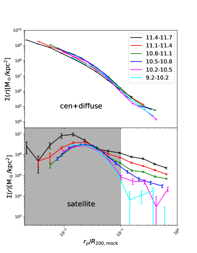
Figure 3: Projected stellar mass density profiles of ICGs $+$ their stellar halos (top) and of satellites (bottom), centered on ICGs in different stellar mass bins (stellar mass taken from SDSS). The log stellar mass ranges are shown by the legend. Errorbars are based on the 1-$\sigma$ scatters of 100 boot-strap subsamples. The gray shaded region in the bottom panel marks the radial range where the satellite profiles are significantly affected by deblending issues.

The projected stellar mass density profiles are presented in Figure 3, for ICGs grouped into a few different stellar mass bins. Hereafter, we call the projected stellar mass density profiles in short as profiles. The profiles of ICGs $+$ their extended stellar halos and of satellites are shown in the top and bottom panels, respectively. The projected distance, $r_{p}$, has been scaled by the halo virial radius (see Table LABEL:tbl:icg), $R_{200,\mathrm{mock}}$, which will be the convention adopted in most of the figures in following sections. In Paper I, we reported that the surface brightness profiles of ICGs and their stellar halos are very similar to each other after scaled by $R_{200,\mathrm{mock}}$, which is particularly true over the stellar mass range of $10.2<\log_{10}M_{\ast}/\mathrm{M}_{\odot}<11.1$. After scaled by $R_{200,\mathrm{mock}}$, the stellar mass density profiles after PSF-deconvolution also become more similar over the stellar mass range of $9.2<\log_{10}M_{\ast}/\mathrm{M}_{\odot}<11.7$, as revealed by the top plot of Figure 3.

The profiles of satellites, on the other hand, show very different trends. As demonstrated by the bottom panel of Figure 3, the profiles centered on more massive ICGs have higher amplitudes after scaling $r_{p}$ by $R_{200,\mathrm{mock}}$ and at $r_{p}/R_{200,\mathrm{mock}}>0.1$, indicating the scaling relation between the stellar mass in satellites and the host halo mass must be different, which we will discuss later in Section 4.2. The profiles of satellites are also more flattened and extended than those of the central ICGs $+$ their stellar halos.

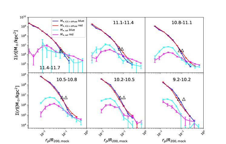
Figure 4: Projected stellar mass density profiles of ICGs $+$ their stellar halos (red and blue) and of satellite galaxies (magenta and cyan), around ICGs with different stellar mass (see the text in each panel). In a given panel, red/magenta and blue/cyan curves show the results around red and blue ICGs, respectively. We only include those satellites with log stellar mass greater than $\log_{10}M_{\ast,\mathrm{ICG}}-3$, i.e., within three orders of difference with respect to the central ICGs. Note the satellite profiles can be significantly affected by deblending mistakes within $0.1R_{200,\mathrm{mock}}$ (see Appendix A). The inner and outer black triangles mark twice the Petrosian radius of red and blue ICGs. Blue ICGs are dominated by less concentrated late-type galaxies, and thus have larger Petrosian radius, but their outer stellar halos are less extended. Errorbars are based on the 1-$\sigma$ scatters of 100 boot-strap subsamples.

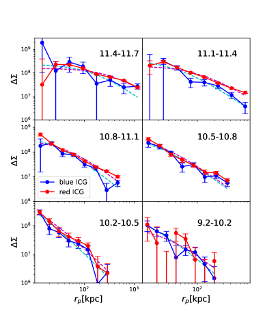
Figure 5: Lensing signals around red and blue ICGs (see the legend) in a few different log stellar mass bins (see the text in each panel). Errorbars are based on the 1-$\sigma$ scatters of 100 boot-strap subsamples. Dashed curves with magenta and cyan colors are the best-fitting NFW model profiles.

In Figure 4, the profiles centered on ICGs with different stellar mass are presented in separate panels. In each panel, ICGs are further split into red and blue populations based on a stellar mass dependent color division of ${}^{0.1}(g-r)<0.065\log_{10}M_{\ast}/\mathrm{M}_{\odot}+0.1$. The profiles of satellite galaxies behave very differently around red and blue ICGs. Beyond $0.1R_{200,\mathrm{mock}}$, where the profiles are not significantly affected by deblending issues, the amplitudes are higher around red ICGs with $\log_{10}M_{\ast}/\mathrm{M}_{\odot}>10.8$. At $\log_{10}M_{\ast}/\mathrm{M}_{\odot}<10.8$, we fail to see significant differences given the noisy measurements.

In an early study, Wang & White (2012) reported that the satellite abundance around red isolated galaxies is higher than those around blue ones with the same stellar mass, which reflects the fact that red central galaxies are hosted by more massive dark matter halos than blue centrals with the same stellar mass. This has been directly confirmed by weak lensing measurements from SDSS (Mandelbaum et al., 2016), and it was found that the difference in satellite abundance and host halo mass between red and blue ICGs both peak at the stellar mass of about $\log_{10}M_{\ast}/\mathrm{M}_{\odot}\sim 11.1$.

With the high quality weak gravitational lensing shear measurements based on the deep and high resolution HSC imaging products, we can measure the lensing signals as a function of the projected radius, $r_{p}$, despite the fact that the footprint of HSC is much smaller than SDSS. The lensing signals are presented in Figure 5. In the top right and middle left panels ($10.8<\log_{10}M_{\ast}/\mathrm{M}_{\odot}<11.4$), the lensing signals around red ICGs are clearly higher in amplitudes. For the most massive stellar mass bin ($11.4<\log_{10}M_{\ast}/\mathrm{M}_{\odot}<11.7$), the middle right panel ($10.5<\log_{10}M_{\ast}/\mathrm{M}_{\odot}<10.8$) and the bottom left panel ($10.2<\log_{10}M_{\ast}/\mathrm{M}_{\odot}<10.5$), there are also indications that the blue curve is below the red one, but the difference is not significant compared with the errorbars. Besides, there are no obvious differences between the red and blue curves in the two bottom panels. Note we do not have enough numbers of blue/red ICGs at the most/least massive ends. Nevertheless, the trends revealed by lensing signals are in good agreement with the results based on satellites in Figure 4, i.e., over the stellar mass range of $10.8<\log_{10}M_{\ast}/\mathrm{M}_{\odot}<11.4$, we clearly detect that red ICGs tend to have more satellites and are hosted by more massive dark matter halos than blue ICGs in the same stellar mass bin.

The profiles of ICGs $+$ their stellar halos in Figure 4 behave differently for red and blue ICGs as well. On small scales, red ICGs tend to have slightly more concentrated profiles than blue ICGs, except for the most massive bin. Such a difference is more obvious for smaller ICGs in the three bottom panels, i.e., the profiles of blue ICGs tend to have higher amplitudes than those of red ICGs at $0.02R_{200}<r_{p}<0.09R_{200}$. The top middle and right panels also show similar but weaker trends. Note in the most massive bin, there is not enough number of blue ICGs, and our conversion from surface brightness profiles to projected stellar mass density profiles might have weakened such a difference.

On larger scales, red ICGs tend to have more extended stellar halos than blue ones. This is in good agreement with previous studies based on both real observations (e.g. D’Souza et al., 2014) and hydrodynamical simulations (e.g. Pillepich et al., 2014; Rodriguez-Gomez et al., 2016). The outer stellar halo is believed to be dominated by stripped stars from satellites, and thus the difference indicates that red passive galaxies accrete more stars than blue star-forming galaxies.

The facts that red centrals have more satellites, more extended stellar halos and are hosted by more massive dark matter halos support the standard theory of structure and galaxy formation, which we will discuss in Section 5. Despite the difference in $M_{200}$ (hence $R_{200}$) for red and blue ICGs at fixed stellar mass, as revealed by weak lensing signals, we scale the projected distance $r_{p}$ to red and blue ICGs using the same $R_{200,\mathrm{mock}}$ in Table LABEL:tbl:icg, without distinguishing by color.

We note in the end that the profiles of satellites around blue ICGs tend to be more concentrated than those around red ICGs for the few inner most data points, which might indicate the stronger tidal disruption around red ICGs in such inner regions. However, as shown in Appendix A, the satellite counts may have been significantly affected by deblending issues within $0.1R_{200,\mathrm{mock}}$. In fact, Wang et al. (2021) have reported that the rich substructures of blue late-type ICGs, such as spiral arms and star-forming regions, can have high possibilities to be mistakenly deblended as companion sources, which result in faked increase in the inner number density profiles of satellites. Proper investigations of the inner satellite profiles require very careful corrections for such deblending issues.

By fitting the NFW profiles to the lensing signals in Figure 5, we are able to recover the best-fitting virial mass, $M_{200}$, for the host halos of ICGs with different stellar mass, which can be used to directly investigate the relations between host halo mass and the total stellar mass in satellites, in ICGs and their extended stellar halos. In the next section, we move on to investigate these scaling relations for red and blue ICGs separately.

4.2 Scaling Relations

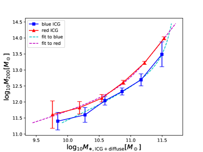
Figure 6: Virial mass for the host halos of ICGs, $M_{200}$, measured from the stacked weak lensing signals in Figure 5, versus the integrated stellar mass for ICGs $+$ their stellar halos. Magenta and cyan dashed curves are best-fitting double power-law functions to the measurements for red and blue ICGs, with the best-fitting parameters provided in Table LABEL:tbl:scaling. If fitting single power-law models to the four most massive data points, the best-fitting results are $M_{200}\propto M_{\ast,\mathrm{ICG+diffuse}}^{2.064\pm 0.080}$ and $M_{200}\propto M_{\ast,\mathrm{ICG+diffuse}}^{2.094\pm 0.512}$ for red and blue ICGs, respectively.

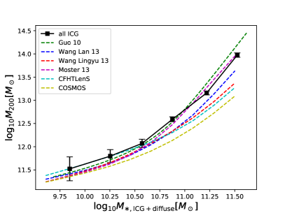
Figure 7: Similar to Figure 6, but black squares with errorbars show the relation of $M_{200}$ versus $M_{\ast,\mathrm{ICG+diffuse}}$ for all ICGs. Dashed curves with different colors are stellar mass versus halo mass relations in a few previous studies (Guo et al., 2010; Leauthaud et al., 2012; Wang et al., 2013b; Moster et al., 2013; Wang et al., 2013a; Hudson et al., 2015).

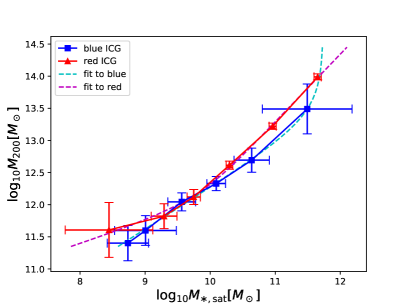
Figure 8: Similar to Figure 6, but $M_{200}$ is shown as a function of the stellar mass in satellites with $\log_{10}M_{\ast,\mathrm{sat}}>\log_{10}M_{\ast,\mathrm{ICG}}-3$ and with projected distance to the central ICGs in between 0.1$R_{200,\mathrm{mock}}$ and $R_{200,\mathrm{mock}}$. ICGs are split into red and blue populations, as indicated by the legend. Magenta and cyan dashed curves are best-fitting double power-law functions to the measurements for red and blue ICGs, with the best-fitting parameters provided in Table LABEL:tbl:scaling. If fitting single power-law models to the four most massive data points, the best-fitting results are $M_{200}\propto M_{\ast,\mathrm{sat}}^{0.976\pm 0.036}$ and $M_{200}\propto M_{\ast,\mathrm{sat}}^{1.017\pm 0.184}$ for red and blue ICGs, respectively.

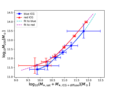
Figure 9: $M_{200}$ as a function of the total stellar mass in satellites and ICGs $+$ their stellar halos. Similar to Figure 8, we only include satellites with $\log_{10}M_{\ast,\mathrm{sat}}>\log_{10}M_{\ast,\mathrm{ICG}}-3$ and with projected distance to the central ICGs in between 0.1$R_{200,\mathrm{mock}}$ and $R_{200,\mathrm{mock}}$. ICGs are split into red and blue populations, as indicated by the legend. Magenta and cyan dashed curves are best-fitting double power-law functions to the measurements for red and blue ICGs, with the best-fitting parameters provided in Table LABEL:tbl:scaling. If fitting single power-law models to the four most massive data points, the best-fitting results are $M_{200}\propto(M_{\ast,\mathrm{sat}}+M_{\ast,\mathrm{ICG+diffuse}})^{1.449\pm 0.041}$ and $M_{200}\propto(M_{\ast,\mathrm{sat}}+M_{\ast,\mathrm{ICG+diffuse}})^{1.676\pm 0.297}$ for red and blue ICGs, respectively.

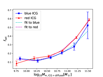
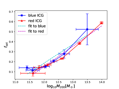
Figure 10: The fraction of stellar mass in satellites versus the total stellar mass in satellites and ICGs $+$ their stellar halos, reported as a function of the stellar mass in ICGs and their stellar halos, $M_{\ast,\mathrm{ICG+diffuse}}$, (left), and as a function of $M_{200}$ (right). Red and blue symbols and curves are for red and blue ICGs, respectively. Magenta and cyan curves are best-fitting cubic polynomial models (left) and power-law models (right) for red and blue ICGs.

The weak lensing mass profiles in Figure 5 are measured and fitted out to $2R_{200,\mathrm{mock}}$, which is close to the halo depletion radius (Fong & Han, 2021) that marks the separation between the one and two halo terms in halo model (e.g., Hayashi & White, 2008; Garcia et al., 2020). For each measured profile we fit a single projected NFW profile (Wright & Brainerd, 2000) with the virial mass, $M_{200}$, and concentration, $c_{200}$, as free parameters. The fitting is done by minimizing the value of $\chi^{2}$ using the software iminuit, which is a python interface of the minuit function minimizer (James & Roos, 1975). We have also tried the emcee software (Foreman-Mackey et al., 2013). The best-fitting NFW profiles and the associated errors by using iminuit and emcee agree well with each other.

In principle, we can directly use $R_{200}$ inferred from weak lensing signals, which are not exactly the same as $R_{200,\mathrm{mock}}$ in Table LABEL:tbl:icg. In fact, $R_{200}$ inferred from weak lensing signals are larger than $R_{200,\mathrm{mock}}$ by about 24%, 9%, 12%, 1.6%, 2.2% and $<$1% from the most to least massive bins. The discrepancy is larger for more massive bins, which is perhaps related to the large scatter in $M_{200}$ at fixed stellar mass for massive halos. However, given the measurement uncertainties, we stick to use $R_{200,\mathrm{mock}}$ in Table LABEL:tbl:icg. It affects how the results are presented in Figures 3 and 4, but does not change the conclusions. As we have checked, the trends in Figures 3 slightly differ, but the conclusion still holds if using $R_{200}$ estimated from weak lensing signals. The other conclusions which are going to be presented in this subsection are not affected at all.

Figure 6 shows the best-fitting virial mass of the host dark matter halo, $M_{200}$, versus the stellar mass of ICGs $+$ their stellar halos, $M_{\ast,\mathrm{ICG+diffuse}}$, which is integrated over the profiles in Figure 4. Note here we choose to use $M_{\ast,\mathrm{ICG+diffuse}}$, instead of the original stellar mass of ICGs measured from the shallower SDSS photometry, which we denote as $M_{\ast,\mathrm{ICG}}$. We only show the vertical errorbars for the best-fitting $M_{200}$ from weak lensing signals, as the errorbars in $M_{\ast,\mathrm{ICG+diffuse}}$ are very small for ICGs in a given stellar mass bin.

It seems $M_{200}$ of red ICGs is on average larger than that of blue ICGs in the same stellar mass bin, but only the second and third massive data points show more than 1-$\sigma$ significance, which is in very good agreement with the trends shown in Figures 4 and 5. At $\log_{10}M_{\ast,\mathrm{ICG+diffuse}}/\mathrm{M}_{\odot}>10.5$, the power-law index is very close to 2 (or $M_{\ast,\mathrm{ICG+diffuse}}\propto M_{200}^{1/2}$). Indeed, for the four most massive data points of red ICGs, where the errorbars are small enough, the best-fitting power-law index is $2.064\pm 0.080$. At $\log_{10}M_{\ast,\mathrm{ICG+diffuse}}/\mathrm{M}_{\odot}<10.5$, on the contrary, the amount of change in host halo mass becomes slower, despite the significant decrease in stellar mass. The general trends are consistent with stellar mass versus halo mass relations measured in previous studies (e.g. Guo et al., 2010; Wang & Jing, 2010; Yang et al., 2012; Leauthaud et al., 2012; Moster et al., 2013; Wang et al., 2013b, a; Hudson et al., 2015).

Following the functional form adopted in Wang & Jing (2010), we model the relation of $M_{200}$ versus $M_{\ast,\mathrm{ICG+diffuse}}$ for red and blue ICGs separately as

$$M_{\ast,\mathrm{ICG+diffuse}}=\frac{2k}{(\frac{M_{200}}{M_{0}})^{-\alpha}+(\frac{M_{200}}{M_{0}})^{-\beta}}.$$ (7)

In order to properly consider the errors in $M_{200}$ for the fitting, Equation 7 is in fact tabulated into values of $M_{200}$ versus $M_{\ast,\mathrm{ICG+diffuse}}$, for a given set of parameters, before fitting to the data points. The best-fitting relations are shown as magenta and cyan dashed curves in Figure 6, for red and blue ICGs respectively. The best-fitting parameters are provided in the first and second rows of Table LABEL:tbl:scaling.

Our results in Figure 6 are consistent with the commonly recognized galaxy formation models. For massive galaxies, a change in stellar mass leads to a more rapid change in host halo mass. In standard galaxy formation theory, AGN feedback is often adopted to prohibit the star-forming activities in massive galaxies, making the growth in stellar mass less efficient, which might explain why with the change in host halo mass, the change in stellar mass is smaller. For galaxies smaller than $\log_{10}M_{\ast,\mathrm{ICG+diffuse}}/\mathrm{M}_{\odot}\sim 10.5$, on the other hand, the slow change in host halo mass indicates that the star formation activities in low-mass halos are significantly more inefficient and stochastic, which depends very weakly on host halo mass.

Table 2: The best-fitting parameters for the scaling relations presented in Figures 6, 8 and 9, and for red and blue ICGs respectively. The model functional form is $X=\frac{2k}{(\frac{M_{200}}{M_{0}})^{-\alpha}+(\frac{M_{200}}{M_{0}})^{-\beta}}$, where $X$ represents $M_{\ast,\mathrm{ICG+diffuse}}$, $M_{\ast,\mathrm{sat}}$ or $M_{\ast,\mathrm{ICG+diffuse}}+M_{\ast,\mathrm{sat}}$. Note the data points around red ICGs tend to have higher amplitudes in corresponding figures, but the best-fitting amplitudes here are lower. This is due to the positive correlation between $\log_{10}k$ and $\log_{10}M_{0}$, and the negative correlation between $\log_{10}k$ and $\beta$.

relation	$\log_{10}M_{0}$	$\alpha$	$\beta$	$\log_{10}k$
$M_{200}$ vs $M_{\ast,\mathrm{ICG+diffuse}}$ (red ICG)	12.14$\pm$0.50	1.69$\pm$1.13	0.39$\pm$0.13	10.51$\pm$0.43
$M_{200}$ vs $M_{\ast,\mathrm{ICG+diffuse}}$ (blue ICG)	12.80$\pm$2.58	1.10$\pm$0.86	0.08$\pm$3.81	11.21$\pm$1.31
$M_{200}$ vs $M_{\ast,\mathrm{sat}}$ (red ICG)	11.97$\pm$0.86	3.00$\pm$5.47	0.95$\pm$0.26	9.45$\pm$1.25
$M_{200}$ vs $M_{\ast,\mathrm{sat}}$ (blue ICG)	13.39$\pm$1.06	1.54$\pm$0.66	0.01$\pm$4.86	11.42$\pm$0.83
$M_{200}$ vs $M_{\ast,\mathrm{ICG+diffuse}}+M_{\ast,\mathrm{sat}}$ (red ICG)	11.80$\pm$0.48	2.67$\pm$1.70	0.65$\pm$0.12	10.18$\pm$0.50
$M_{200}$ vs $M_{\ast,\mathrm{ICG+diffuse}}+M_{\ast,\mathrm{sat}}$ (blue ICG)	12.74$\pm$1.94	1.18$\pm$0.72	0.42$\pm$1.06	11.29$\pm$1.72

Table 3: The best-fitting parameters for $f_{\mathrm{sat}}$ versus $M_{\ast,\mathrm{ICG+diffuse}}$ and $f_{\mathrm{sat}}$ versus or $M_{200}$ in Figure 10, and for red and blue ICGs respectively. The model functional form is demonstrated by Equations 10 and 11.

relation	$a$	$b$	$c$	$d$
$f_{\mathrm{sat}}$ vs $M_{\ast,\mathrm{ICG+diffuse}}$ (red ICG)	28.4658$\pm$0.0876	$-$67.6943$\pm$0.1190	49.6482$\pm$0.1304	$-$10.3045$\pm$0.1135
$f_{\mathrm{sat}}$ vs $M_{\ast,\mathrm{ICG+diffuse}}$ (blue ICG)	26.4056$\pm$0.1666	$-$64.7616$\pm$0.2164	49.7637$\pm$0.2283	$-$11.2813$\pm$0.1928
$f_{\mathrm{sat}}$ vs $M_{200}$ (red ICG)	0.204$\pm$0.016	$-$2.296$\pm$0.205	–	–
$f_{\mathrm{sat}}$ vs $M_{200}$ (blue ICG)	0.188$\pm$0.033	$-$2.068$\pm$0.403	–	–

Figure 7 shows a more detailed comparison of the stellar mass versus halo mass relation for all ICGs against the measurements in a few previous studies, which are either based on abundance matching and HOD (Halo Occupation Distribution) modelling (Guo et al., 2010; Wang & Jing, 2010; Moster et al., 2010, 2013; Wang et al., 2013b, a) or based on modelling lensing signals of other surveys (Leauthaud et al., 2012; Hudson et al., 2015). Note all the HOD based studies are measuring the stellar mass for halos at a given mass, whereas we are measuring the halo mass for ICGs in a given stellar mass bin through stacked lensing. Thus we make the following conversion (Han et al., 2015b)

$$\log_{10}M_{\mathrm{halo}}(M_{\ast})=\int\log_{10}M_{\mathrm{halo}}\mathrm{d}P(M_{\mathrm{halo}}|M_{\ast}),$$ (8)

where $\mathrm{d}P(M_{\mathrm{halo}}|M_{\ast})$ is defined as

$$\mathrm{d}P(M_{\mathrm{halo}}|M_{\ast})=\frac{\mathrm{d}P(M_{\ast}|M_{\mathrm{halo}})\phi(M_{\mathrm{halo}})\mathrm{d}M_{\mathrm{halo}}}{\int\mathrm{d}P(M_{\ast}|M_{\mathrm{halo}})\phi(M_{\mathrm{halo}})\mathrm{d}M_{\mathrm{halo}}}.$$ (9)

$\phi(M_{\mathrm{halo}})$ in Equation 9 is the halo mass function. The distributions/scatters of stellar mass at fixed halo mass $P(M_{\ast}|M_{\mathrm{halo}})$ are taken from the original studies. Our measurement appears to be closest to Guo et al. (2010) and Moster et al. (2013) models, but the other models tend to show lower amplitudes than the black squares. The dashed color curves show large variations from each other, which are mostly due to the different amount of HOD scatter assumed in each model. If assuming the same amount of scatter of 0.2 dex, the discrepancy would become smaller (Han et al., 2015b) among these models, and most of their amplitudes are still lower than that of the black squares at $\log_{10}M_{\ast,\mathrm{ICG+diffuse}}>10.6$.

The difference between our measurements and many of the previous studies can NOT be explained by the fact that we adopted $M_{\ast,\mathrm{ICG+diffuse}}$, while these previous studies did not carefully consider the stellar mass contained in the outer stellar halo. Their stellar mass is expected to be lower than our $M_{\ast,\mathrm{ICG+diffuse}}$ at the massive end (see Appendix C for details), so the tension would only become larger if considering such a difference in stellar mass.

This could be related to the sample selection, as the ICGs used in this study is a flux limited sample, which will introduce slightly over-estimated halo mass than using a volume limited sample (Han et al., 2015b). However, after including volume corrections to our sample of ICGs, the amount of change is at most about $-$0.04 dex in $M_{200}$, which is far from enough to explain the difference. The other more important aspect is the scatter/dispersion in halo mass at fixed stellar mass in our analysis. Mandelbaum et al. (2005) reported that the best recovered halo mass through stacked lensing signals lies in between the actual mean and median values. Proper comparisons between our halo mass measurements and previous studies require careful calibrations of the bias introduced by such mass dispersions. A 0.5/0.7 dex of dispersion in halo mass would cause a bias from the median as large as $\sim-$0.17/$-$0.32 dex(Han et al., 2015b). Checked against the mock galaxy catalog of Guo et al. (2011b), the typical scatter of halo mass in the three most massive stellar mass bins in our analysis ranges from 0.33 to 0.41 dex. Thus the halo mass dispersion may help to explain part of the difference at the massive end. The remaining source of uncertainties is at least partly contributed by the amount of assumed HOD scatter in Equation 8.

Figure 8 shows $M_{200}$ versus the integrated stellar mass in satellites, $M_{\ast,\mathrm{sat}}$. $M_{\ast,\mathrm{sat}}$ is integrated over the radial range of $0.1R_{200,\mathrm{mock}}<r_{p}<R_{200,\mathrm{mock}}$ in Figure 4. Here we adopt an inner radius cut of $0.1R_{200,\mathrm{mock}}$ to avoid the region significantly affected by deblending mistakes, though the integrated stellar mass in satellites is expected to be dominated by the mass in the outer region and thus might not be sensitive to the inner profiles. Besides, only satellites with $\log_{10}M_{\ast}>\log_{10}M_{\ast,\mathrm{ICG}}-3$ are included, and thus in principle, $M_{\ast,\mathrm{sat}}$ is a lower limit. Despite this, as long as the faint-end slopes of satellite luminosity functions are shallower than $-2$, satellites smaller than $\log_{10}M_{\ast}\sim\log_{10}M_{\ast,\mathrm{ICG}}-3$ are unlikely to contribute a significant fraction to the total stellar mass in satellites. However, the readers may argue that the chosen mass limit for satellites depends on the stellar mass of ICGs, which might include some artificial dependence on the properties of central ICGs. We think the total stellar mass in satellites below the cut is small anyway, but we have repeated our analysis by choosing a fixed cut in stellar mass, and our conclusions in the following remain the same.

There is a very tight correlation between $M_{200}$ and $M_{\ast,\mathrm{sat}}$. Compared with the $M_{200}$ versus $M_{\ast,\mathrm{ICG+diffuse}}$ relation, the relation between $M_{200}$ and $M_{\ast,\mathrm{sat}}$ shows much weaker dependence on the color of ICGs. The best-fitting power-law index based on the four most massive data points of red ICGs at $\log_{10}M_{\ast,\mathrm{sat}}>10$ (or $\log_{10}M_{\ast,\mathrm{ICG+diffuse}}/\mathrm{M}_{\odot}>10.5$) is $0.976\pm 0.036$, which is very close to 1, i.e., $M_{\ast,\mathrm{sat}}\propto M_{200}$. In addition, we also fit Equation 7 to Figure 8, and the best-fitting parameters are provided in Table LABEL:tbl:scaling. The power-law index is nearly twice of that between $M_{\ast,\mathrm{ICG+diffuse}}$ and $M_{200}$. This implies that with the same amount of change in host halo mass, the change in the total stellar mass locked in satellites is more rapid than the change in the total stellar mass in central ICGs at $\log_{10}M_{\ast,\mathrm{ICG+diffuse}}/\mathrm{M}_{\odot}>10.5$.

Interestingly, we can see some indications that there are slightly more stellar mass locked in satellites around blue ICGs at $\log_{10}M_{200}/\mathrm{M}_{\odot}>12.7$, but the errorbars are also very large and the difference is only marginal at $\log_{10}M_{200}/\mathrm{M}_{\odot}\sim 12.7$. This perhaps indicates the late formation time of blue galaxies, and hence retaining more substructures and satellites. However, considering the fact that the best-fitting $M_{200}$ are achieved through binning in stellar mass, while red and blue ICGs at fixed stellar mass can have different scatters in $M_{200}$, we do not make a very strong conclusion here.

For completeness, we show in Figure 9 the halo mass, $M_{200}$, versus the total stellar mass in satellites and central ICGs $+$ their stellar halos, $M_{\ast,\mathrm{sat}}+M_{\ast,\mathrm{ICG+diffuse}}$. Based on the four most massive data points of red ICGs, the best-fitting power-law index is $1.449\pm 0.041$ ($M_{\ast,\mathrm{sat}}+M_{\ast,\mathrm{cen+diffuse}}\propto M_{200}^{1/1.449}$). The best-fitting parameters based on Equation 7 are provided in Table LABEL:tbl:scaling. The power-law index is in between that of $M_{\ast,\mathrm{ICG+diffuse}}$ versus $M_{200}$ and that of of $M_{\ast,\mathrm{sat}}$ versus $M_{200}$, and is expected to depend on the fraction of stellar mass locked in satellites.

The left plot of Figure 10 shows the fraction of stellar mass in satellites versus the total stellar mass in satellites and ICGs $+$ their stellar halos, $f_{\mathrm{sat}}$, reported as a function of $M_{\ast,\mathrm{ICG+diffuse}}$, while the right plot shows the same fraction as a function of $M_{200}$.

In both plots, $f_{\mathrm{sat}}$ increases with the increase in $M_{\ast,\mathrm{ICG+diffuse}}$ and $M_{200}$ for the four most massive data points. $f_{\mathrm{sat}}$ can be as high as 50–60% at the massive end, in general consistency with previous studies based on galaxy clusters (Gonzalez et al., 2013; Furnell et al., 2021, e.g.), predictions by hydro-dynamical simulations (Puchwein et al., 2010; Cui et al., 2014, e.g.) and HOD modelling(e.g. Yang et al., 2009), though in these previous studies, there are still some tensions between observational constraints and predictions by simulations. For MW-mass galaxies, $f_{\mathrm{sat}}$ drops to slightly more than $\sim 10\%$. At the low-mass end of the left plot, $f_{\mathrm{sat}}$ is nearly flat, again indicating the more stochastic star formation of low-mass galaxies and also the stochastic accretion of low-mass satellites by low-mass central ICGs. Interestingly, in contrast to the slow change of $M_{200}$ with the decrease in both $M_{\ast,\mathrm{ICG+diffuse}}$ and $M_{\ast,\mathrm{sat}}$, $f_{\mathrm{sat}}$ tends to have a more linear relation with $M_{200}$ in the right plot, though the best-fitting $M_{200}$ is quite noisy at the low-mass end.

In the left plot, $f_{\mathrm{sat}}$ is higher around red ICGs than blue ICGs at fixed stellar mass, except for the least massive bin. The trends are self-consistent and can be explained by the fact that red galaxies sit in denser environments of our Universe and thus accrete more massive satellites.

Interestingly, the right plot of Figure 10 reveals that the fractions of stellar mass in satellites around red and blue ICGs are similar, but at $\log_{10}M_{200}/\mathrm{M}_{\odot}>12.7$, it seems $f_{\mathrm{sat}}$ is slightly lower for red ICGs than blue ICGs hosted by dark matter halos with the same $M_{200}$. This perhaps tells that the fraction of stellar mass in satellites is mainly determined by the host halo mass, while in agreement with Figure 8, it probably also reflects the late formation of blue galaxies, which is a secondary factor compared with the host halo mass. However, the difference is not significant compared with the errorbars.

We also provide the best-fitting relations of $f_{\mathrm{sat}}$ versus $M_{\ast,\mathrm{ICG+diffuse}}$ or $M_{200}$. Cubic polynomial model is adopted to fit the relation between $f_{\mathrm{sat}}$ and $M_{\ast,\mathrm{ICG+diffuse}}$

$$f_{\mathrm{sat}}= a\left(\frac{\log_{10}M_{\ast,\mathrm{ICG+diffuse}}}{10}\right)^{3}+b\left(\frac{\log_{10}M_{\ast,\mathrm{ICG+diffuse}}}{10}\right)^{2}$$ (10)

$$+c\left(\frac{\log_{10}M_{\ast,\mathrm{ICG+diffuse}}}{10}\right)+d,$$

while single power-law model is adopted to fit the relation between $f_{\mathrm{sat}}$ and $M_{200}$

$$f_{\mathrm{sat}}=a\log_{10}M_{200}+b.$$ (11)

The best-fitting parameters are provided in Table LABEL:tbl:scaling2.

4.3 Radial dependence of the total stellar mass fraction

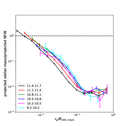
Figure 11: Total stellar mass (stellar mass in satellites and ICGs $+$ their stellar halos) versus total mass (the best-fitting NFW model profiles through weak lensing signals), as a function of $r_{p}/R_{200,\mathrm{mock}}$ and for ICGs in different stellar mass bins. The black dashed horizontal line marks the value of unity. Errorbars include the contribution from three different parts: (i) the boot-strap errors of satellite profiles; (ii) the boot-strap errors of ICG $+$ stellar halo profiles; (iii) uncertainties in the best-fitting NFW model. (i), (ii) and (iii) are all propagated to the final errors.

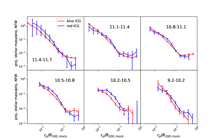
Figure 12: Similar to Figure 11, but shows the radial distribution for the fraction of total stellar mass versus total mass for red and blue ICGs separately. ICGs in different stellar mass bins are presented in different panels, as indicated by the text in each panel. Errorbars are calculated in the same way as Figure 11.

So far we have investigated the scaling relations of $M_{200}$ versus $M_{\ast,\mathrm{ICG+diffuse}}$, $M_{\ast,\mathrm{sat}}$ and versus $M_{\ast,\mathrm{ICG+diffuse}}+M_{\ast,\mathrm{sat}}$. These are based on the integrated mass. With the measured mass profiles, we are able to more closely investigate the total stellar mass fraction as a function of the projected distance to ICGs.

Figure 11 and 12 show the projected total stellar mass density profiles ($M_{\ast,\mathrm{ICG+diffuse}}$ $+$ $M_{\ast,\mathrm{sat}}$ profiles), divided by the best-fitting projected NFW density profiles based on weak lensing signals in Figure 5. Figure 11 is based on all ICGs, while in Figure 12 we further divide ICGs into red and blue subsamples. Note the inner satellite profiles within $0.1R_{200,\mathrm{mock}}$ are affected by deblending issues and are thus not reliable. However, in such inner regions, the profiles are dominated by the central ICGs, and thus the summation of the two is not sensitive to deblending mistakes.

In both figures, uncertainties of the satellite profiles, of the profiles of ICGs $+$ their stellar halos and of the best-fitting NFW profiles through the lensing signals are all considered and propagated to the final errorbars. The uncertainties of the best-fitting NFW profiles are estimated from the boundaries which enclose 68% of the MCMC chains.

In Figure 11, high and low-mass ICGs tend to have different stellar mass fractions, in terms of both the shapes and amplitudes. There is nearly a monotonic trend that less massive ICGs tend to have lower fractions over $0.02R_{200,\mathrm{mock}}<r_{p}<0.1R_{200,\mathrm{mock}}$, except for the magenta and blue curves. This is partly related to the fact that massive ICGs are dominated by elliptical galaxies with de Vaucouleurs profiles and are thus more centrally concentrated. On the other hand, low-mass ICGs are dominated by exponential profiles and are more extended. Thus less massive ICGs tend to have less stellar mass in central regions but more stellar mass at intermediate radii. In addition, the fact that ICGs with $10.5<\log_{10}M_{\ast}/\mathrm{M}_{\odot}<10.8$ seem to show higher amplitudes beyond 0.02$R_{200,\mathrm{mock}}$ than ICGs in the other neighboring bins probably indicate that $M_{\ast}/M_{200}$ peaks for MW-mass galaxies (e.g. Guo et al., 2010). Note the measurement in the least massive bin (cyan curve) might be too noisy.

In Figure 12, blue ICGs tend to have higher stellar mass fractions between $0.02R_{200,\mathrm{mock}}$ and $0.1R_{200,\mathrm{mock}}$. The trend is also related to the fact that blue star-forming galaxies are dominated by exponential profiles and are thus more extended. Besides, this might imply the higher star formation efficiency per unit halo mass for blue star-forming galaxies.

In both Figure 11 and 12, the values of a few inner most data points are larger than one. This likely reflects deviations from the NFW profile in the very inner region, where baryons dominate. The fractions keep dropping with the increase in projected distance to the central ICG up to $\sim 0.15R_{200,\mathrm{mock}}$. Interestingly, we can see the profiles go almost flat beyond $\sim 0.15R_{200,\mathrm{mock}}$, and the place where the profiles start to go flat is almost the same after scaling $r_{p}$ by $R_{200,\mathrm{mock}}$. This reflects the transition radius from ICG dominated regions to satellite dominated regions.

In the satellite dominated region beyond the transition radius, the stellar mass versus total mass fractions are all below 1%. The nearly flat profiles indicate the radial distribution of satellites tend to trace the distribution of dark matter, in good agreement with previous studies (e.g. Wang et al., 2018). In Figure 12, blue massive and red low-mass ICGs tend to have noisy measurements, which is due to the small number of galaxies with corresponding colors in these bins. There are some small differences between the red and blue curves in the satellite dominated region, but the trend is not monotonic. Red ICGs tend to have lower stellar mass fractions than blue ICGs in the second and third massive bins, but higher fractions in the most massive, fourth and fifth bins. Measurements in the least massive bin is too noisy (see Figure 5). Given the large errorbars and noisy measurements, we avoid making strong conclusions.

Unfortunately, due to deblending issues, we are unable to have decent comparisons between the radial distribution of stellar mass in diffuse stellar halos and satellites. This is because beyond $0.1R_{200,\mathrm{mock}}$, where the results are not significantly affected by deblending mistakes, we have at most one to two data points for the profiles of the outer stellar halos. The radial range where we have good measurements for both satellites and ICGs $+$ their stellar halos, while not sensitive to deblending mistakes, is very limited. We thus postpone such a comparison to future studies.

5 Conclusions and discussions

In this study, we measured the projected stellar mass density profiles for satellite galaxies as a function of the projected distance to the center of isolated central galaxies (ICGs) and for ICGs themselves $+$ their extended stellar halos. The profiles of satellites are measured by counting photometric companions from the deep Hyper Suprime-Cam (HSC) imaging survey and with statistical fore/background subtraction. The profiles of ICGs $+$ their stellar halos are obtained by stacking galaxy images from HSC to push beyond the noise limit of individual images.

The signals can be successfully measured around ICGs spanning a wide range in stellar mass ($9.2<\log_{10}M_{\ast}/\mathrm{M}_{\odot}<11.7$) and out to the virial radius ($R_{200,\mathrm{mock}}$), which demonstrate the power of the deep HSC survey. Despite the fact that the footprint of HSC is significantly smaller than that of SDSS, we are able to achievement measurements for ICGs that are smaller by one order of magnitude in stellar mass than previous studies based on SDSS.

We found red ICGs tend to have less extended inner profiles within 0.1$R_{200,\mathrm{mock}}$, and more extended outer stellar halos. Over the radial range not affected by source deblending issues, the stellar mass density profiles of satellites have higher amplitudes around red ICGs than blue ICGs with the same stellar mass, in good agreement with previous studies (e.g. Wang & White, 2012; Wang et al., 2014), which have reported higher satellite abundance around red ICGs. Weak lensing signals reveal that red ICGs are hosted by more massive dark matter halos than blue ICGs with the same stellar mass, and such a difference peaks at about $\log_{10}M_{\ast}/\mathrm{M}_{\odot}\sim 11.1$, indicating the satellite abundance and total stellar mass locked in satellites are good proxies to the host halo mass.

Under the standard picture of cosmic structure formation, red galaxies formed early and grew fast at early epochs. The rapid star formation trigerred feedback mechanisms heating the surrounding gas. As a result, late-time star-forming activities are prohibited due to the lack of cold gas supply, while their host dark matter halos, outer stellar halos and the population of satellites keep growing through accretion. Because red galaxies are on average found in more over-dense regions than blue galaxies, they probably even accrete more dark matter and more massive satellites. On the other hand, star forming galaxies are blue. Thus at fixed host halo mass, we expect red passive galaxies, whose star forming activities were quenched a long time ago, to be smaller in stellar mass. In other words, if the stellar mass is the same, red galaxies are hosted by more massive dark matter halos and have more satellites.

We revealed a tight correlation between the stellar mass in satellites, $M_{\ast,\mathrm{sat}}$, and the best-fitting host halo mass through weak lensing signals, $M_{200}$, with best-fitting power-law index very close to 1 at $\log_{10}M_{\ast,\mathrm{ICG+diffuse}}/\mathrm{M}_{\odot}>10.5$, i.e., $M_{\ast,\mathrm{sat}}\propto M_{200}$. On the other hand, the scaling relation between the stellar mass in ICGs $+$ their stellar halos and $M_{200}$ is very different, and the best-fitting relation has a power-law index close to $1/2$ at $M_{\ast,\mathrm{ICG+diffuse}}>10.5$, i.e., $M_{\ast,\mathrm{ICG+diffuse}}\propto M_{200}^{1/2}$. Thus with the same amount of increase in $M_{200}$, $M_{\ast,\mathrm{sat}}$ increases faster than $M_{\ast,\mathrm{ICG+diffuse}}$.

At $M_{\ast,\mathrm{ICG+diffuse}}<10.5$, with the decrease in $M_{\ast,\mathrm{ICG+diffuse}}$, the change in host halo mass is slow. This indicates the star-forming activities in low-mass galaxies is inefficient and stochastic, and the accretion of low-mass satellites by low-mass central ICGs is perhaps also more stochastic than that of more massive galaxies.

The difference between the scaling relations of $M_{200}$ versus $M_{\ast,\mathrm{sat}}$ and of $M_{200}$ versus $M_{\ast,\mathrm{ICG+diffuse}}$ can be intuitively understood under the framework of the standard cosmic structure formation theory. As have been mentioned, the host dark matter halo grows in mass and size through accretion. Smaller halos, after being accreted, become subhalos and satellites. In principle, the total stellar mass in satellites can be affected by many factors. For example, satellites can continue forming stars after being accreted by the host dark matter halo, and their stellar material can be stripped after infall. However, if we make a few assumptions: i) the majority of stars are formed before infall; ii) tidal stripping can be ignored, or the amount of stripped stellar mass is on average proportional to the stellar mass formed before infall; iii) at fixed host halo mass, the fraction of stellar mass show reasonable scatter around the mean, it is then not difficult to expect that, statistically, the total stellar mass in satellites is approximately proportional to the total accreted dark matter by the host halo. We also note that for low-mass galaxies, the scatter in stellar mass is huge at fixed halo mass based on previous abundance matching studies (e.g. Guo et al., 2010; Wang & Jing, 2010), which reflects the more stochastic star formation in low-mass galaxies and explains why at $\log_{10}M_{\ast,\mathrm{ICG+diffuse}}/\mathrm{M}_{\odot}<10.5$, $M_{200}$ changes little with the decrease in $M_{\ast,\mathrm{sat}}$. For central galaxies, the growth in stellar mass is contributed by both in-situ star formation and ex-situ accretion of stars from satellites, and the in-situ star formation is regulated by different physical mechanisms, such as the AGN feedback for massive galaxies and more stochastic and inefficient star formation for low mass galaxies as discussed above. Thus the two populations of galaxies, centrals and satellites, are expected to follow very different stellar mass and host halo mass relations.

It would be interesting to investigate the total accreted stellar mass, i.e., those locked in surviving satellites and those accreted stars which have already been stripped from their parent satellites and are currently in the outer stellar halo. Observationally, the calculation of the latter is often achieved through multi-component decomposition of galaxy images or surface brightness profiles (e.g. D’Souza et al., 2014; Oh et al., 2017). However, purely image based two-component decomposition might be dangerous, because the outer component is determined by the few outer most data points, which could be sensitive to systematic uncertainties. We postpone more detailed investigations to future studies, in which we plan to at first validate the decomposition by conducting multi-component fitting to synthetic images based on numerical simulations.

Interestingly, we found indications that blue ICGs tend to have slightly more stellar mass in satellites and also higher fractions of stellar mass in satellites versus total stellar mass ($f_{\mathrm{sat}}$) at $M_{200}\sim 10^{12.7}\mathrm{M}_{\odot}$. If robust, this perhaps indicates the late formation time of blue ICGs. $f_{\mathrm{sat}}$ increases with the increase of $M_{\ast,\mathrm{ICG+diffuse}}$ at $M_{\ast,\mathrm{ICG+diffuse}}>10.5$, which is close to 60% at $\log_{10}M_{\ast}/\sun>11.4$ and drops to $\sim$10% for MW-mass galaxies. At $M_{\ast,\mathrm{ICG+diffuse}}<10.5$, on the other hand, $f_{\mathrm{sat}}$ almost does not change with the decrease in $M_{\ast,\mathrm{ICG+diffuse}}$, again implying the more stochastic star formation of low-mass galaxies and the stochastic accretion of low-mass satellites by low-mass central ICGs. In comparison, the relation between $f_{\mathrm{sat}}$ and $M_{200}$ is more linear over the whole mass range probed.

Our measurements reveal that central ICGs $+$ their stellar halos dominate within $\sim 0.15R_{200,\mathrm{mock}}$, and $\sim 0.15R_{200,\mathrm{mock}}$ marks the start of a transition radius into the satellite dominated region. The fractions of total stellar mass versus total mass are the highest in the galaxy center, which keep dropping with the increase in projected distances to the central ICGs up to $\sim 0.15R_{200,\mathrm{mock}}$. At $r_{p}>0.15R_{200,\mathrm{mock}}$, the stellar mass versus total mass fractions are all below 1%, and stay almost as a constant, indicating the radial distribution of satellites tend to trace the distribution of the underlying dark matter.

In this study, issues related to source deblending within $r_{p}\sim 0.1R_{200,\mathrm{mock}}$ prevent us from proper comparisons between the profiles of ICGs $+$ their stellar halos and that of satellites. We leave more careful corrections for improper source deblending and multi-component image decomposition, as have been discussed above, to future studies. Besides, we did not explicitly distinguish morphology and color in Paper I and this study, and it would be interesting to extend our studies to galaxies such as the red spiral galaxies (e.g. Bundy et al., 2010; Hao et al., 2019), in order to take a closer look at the morphological evolution and its connection to the quench of star-forming activities and the connection to the host dark matter halos. We also plan to extend our studies on satellite galaxies, centrals $+$ stellar halos and their host dark matter halos to intermediate and high redshifts.

Appendix A Source deblending issues

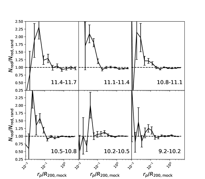
Figure 13: Projected stellar mass density profiles of red background galaxies with $r<25$ around ICGs, divided by the same profiles centered on random points. Measurements on small scales within 0.1$R_{200,\mathrm{mock}}$ tend to be significantly affected by source deblending issues.

On scales close to the central ICGs, companion sources might blend with the footprint of the central galaxy and have to be deblended. However, the radial distribution of satellites may still suffer from imperfect deblending on scales close to the central dominating ICG. This not only affects satellite counts on small scales, but also the surface brightness profiles of ICGs and their stellar halos could be affected if companion sources are not properly detected and thoroughly masked (see Section 3.2). For the latter, the problem is less significant because ICGs dominate over smaller companion galaxies. The amplitudes and slopes of the projected density profiles for satellites, however, may be significantly affected on small scales.

Tal et al. (2012) corrected their satellite counts on small scales, by modelling the smooth light distribution of their sample of luminous red galaxies, subtracting it from the image and detecting remaining sources again. Throughout this paper, we choose to ignore this issue, by focusing on the radial range which is not affected by deblending issues. This is mainly because of the difficulties of modelling the light distribution of late-type galaxies, which have rich star-forming regions and substructures. The choice, however, prevents us from detailed comparison between the radial distribution of satellites, centrals and the diffuse stellar halos on scales affected by deblending issues for now. We postpone more detailed corrections for deblending issues to future studies.

To pick up a reasonable inner radius, outside which the satellite counts are not affected by deblending issues, we count background companions around our ICGs, by using those very red companions with ${}^{0.1}(g-r)>0.065\log_{10}M_{\ast}/\mathrm{M}_{\odot}+0.35$. Based on their color, if they are real galaxies instead of faked sources due to deblending mistakes, it is very unlikely that they stay at the same redshift of the central ICGs. These background counts are divided by the counts around random points, and after the division the ratios are expected to scatter around unity. Any systematic deviation from unity on small scales mainly reflects issues associated with imperfect source deblending. Note source blending happens for fore/background sources as well, which does not depend on whether the companion is a true satellite or a background source.

The results are shown in Figure 13. To ensure enough number of sources on small scales, we use all red background sources down to $r=25$. On large scales, the profiles are consistent with unity, whereas on small scales close to the central parts of ICGs, the profiles deviate from unity, revealing the deblending issues.

In addition to the negative values in the very center, which is probably due to the lacking in sources within such small projected areas, we see significant positive signals at $r_{p}/R_{200,\mathrm{mock}}<0.1$. We have checked that this cannot be explained by lensing magnifications, which contribute much weaker signals. The positive signals could be mainly due to deblending mistakes that parts of the central ICG are mistakenly deblended to be companions. In addition, we cannot rule out the possibility that maybe a very small fraction of real but extremely red satellites may also contribute to such positive signals. Despite this, our discussions throughout the main test are focused on the radial region where the profiles are not significantly affected by deblending issues ($r_{p}>0.1R_{200,\mathrm{mock}}$).

Appendix B PSF correction

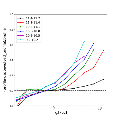
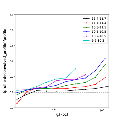
Figure 14: The fractions in the measured surface brightness profiles which are contaminated by PSF scattered light for blue (left) and red (right) ICGs in HSC $r$-band, reported as functions of the projected radius to the galaxy center, and for ICGs in different log stellar mass bins (see the legend).

In paper I, we measured the extended PSF wings out to $\sim 100\arcsec$. Direct deconvolution of the PSF is difficult due to noise, and we obtain the PSF-free surface brightness profiles by fitting PSF-convolved triple Sersic model profiles to the measured surface brightness profiles of ICGs and their stellar halos (Szomoru et al., 2010; Tal & van Dokkum, 2011).

It has been shown by Szomoru et al. (2010) that the residual added best-fitting models are not sensitive to variations in the model parameters and is less model dependent, which can be used as estimates of the PSF-deconvolved profiles, and thus we call them the PSF-corrected profiles.

Figure 14 shows the estimated fractions of PSF contamination in HSC $r$-band, for red and blue ICGs. Consistent with Paper I, the fraction becomes more significant at larger radii and around smaller galaxies, where the outer stellar halos are significantly fainter. In addition, Figure 14 shows that the PSF contamination has a strong dependence on galaxy color. Red galaxies tend to be contaminated less by PSF scattered light at a fixed radius.

The fractions of PSF contamination have been measured for HSC $g$, $r$ and $i$-bands, but for brevity the $g$ and $i$-bands results are not shown. We then correct for the effect of PSF in all three bands, using the fraction of PSF contamination for galaxies with the corresponding stellar mass and color. Note, the fraction of PSF contamination estimated above is based on stacked profiles, which is on average valid for all galaxies in the same bin, whereas there are scatters at individual galaxy level. However, we believe our averaged profiles are statistically correct. We can test in the following way. The PSF correction is at first done using the PSF contamination fraction estimated from the stacked profile of all ICGs in a given stellar mass bin (this is not directly shown in this paper), and then the correction is achieved for red and blue ICGs in the same bin separately, using the corresponding fractions for red and blue (Figure 14). We found the PSF-corrected profiles are almost identical.

Appendix C Validating the recovered stellar mass

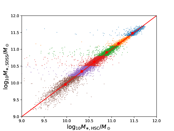
Figure 15: The original stellar mass from SDSS ($y$-axis) versus the recovered stellar mass through GPR ($x$-axis), for SDSS spectroscopic Main galaxies within the HSC footprint. The recovered stellar mass values are based on the ${}^{0.1}(g-r)$ and ${}^{0.1}(r-i)$ colors measured from HSC images and are measured within twice the Petrosian radius, defined by SDSS.

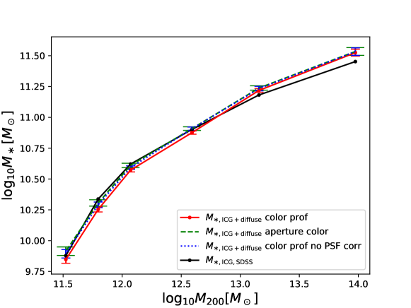
Figure 16: Stellar mass defined in a few different ways, reported as functions of the best-fitting $M_{200}$ from weak lensing signals. Black dots connected by lines are the original stellar mass from SDSS (NYU-VAGC). Red dots connected by solid lines are the integrated stellar mass over the measured stellar mass density profiles of ICGs $+$ their stellar halos, and are based on radius dependent color profiles to infer $M_{\ast}/L_{r}$. Green dashed lines are similar to the red solid one, but a single aperture color is adopted to infer $M_{\ast}/L_{r}$. PSF correction has been included for both red and green symbols. Blue dotted lines are similar to the red solid one, but without PSF correction. Note for the stellar mass from SDSS, each black dot represents the median value for ICGs in the same bin. Mean values lead to slightly different results, but the trends and comparisons among different curves remain the same.

For each galaxy image in HSC $gri$-bands, we mask companion sources using a combination of different source detection thresholds as introduced in Section 3.2. After masking companions, we calculate the Petrosian flux of the ICG, which is defined as the total flux within twice the Petrosian radius, and the Petrosian radius is adopted from SDSS to ensure fair comparisons with SDSS. After applying GPR fitting, the recovered stellar mass is plotted as the $x$-axis quantity of Figure 15, while the $y$-axis shows the original stellar mass from SDSS. Note the SDSS stellar mass is measured by SED fitting to the $ugriz$ Petrosian flux/magnitude.

It is encouraging to see that the stellar mass recovered from HSC images with GPR agree very well with the original SDSS stellar mass in the six stellar mass bins (different color), with the mean stellar mass almost unbiased (red dots). The scatter is flux dependent, ranging from $<0.1$ dex at the bright end to $\sim 0.2$ dex at the faint end. This test not only helps to check the performance of GPR fitting, but it also reflects the difference between SDSS and HSC photometry within the same aperture. The response curves of HSC $g$, $r$ and $i$ filters are almost the same as SDSS. However, HSC is significantly deeper and has smaller PSF size. The way of sky background subtraction and image masks can be quite different between HSC and SDSS. Despite of these differences, we have validated that we can recover the stellar mass in an unbiased way.

In Figure 16, we show the stellar mass versus halo mass relation, for stellar mass calculated in a few different ways. The black solid curve corresponds to the original SDSS (NYU-VAGC) stellar mass. The red solid curve is based on the integrated stellar mass over the projected stellar mass density profiles in Figure 3. The green dashed curve is similar to the red solid one, but to calculate the projected stellar mass density profile, instead of using the actual color profiles, we calculate the average color within twice the SDSS Petrosian radius, and apply the aperture color to the whole radial range to calculate the $M_{\ast}/L_{r}$.

Comparing the original SDSS stellar mass with the integrated stellar mass of the red solid curve, it is clearly shown that at the massive end, the integrated stellar mass is larger than that of SDSS. At the most massive end, the difference is about 0.07 dex. This is mainly because SDSS is shallower, and the signals of the outer stellar halo are failed to be detected on individual SDSS images, while after stacking deep HSC images for galaxies in the same stellar mass bin, we are not only able to go deeper for the same ICG, but also the background noise level is significantly decreased after stacking, which enables us to detect signals below the noise level of individual images.

At the low-mass end, the red solid curve is below the black solid one. This is caused by the radial dependence of $M_{\ast}/L_{r}$. The stellar mass of SDSS was obtained through SED fitting to galaxy colors measured within twice the Petrosian radius. In other words, the same aperture color was applied to obtain an overall $M_{\ast}/L_{r}$ without considering the color gradient. Smaller galaxies have steeper color gradients, and if adopting a fixed aperture color measured closer to the center of the galaxy, $M_{\ast}/L_{r}$ tends to be over-estimated, which explains the difference between the red solid and green dashed curves for smaller ICGs, since the central part of galaxy is redder and the $M_{\ast}/L_{r}$ is larger for red galaxies than blue ones.

The blue dotted curve is similar to the red solid one, but without including PSF corrections, and it seems the integrated stellar mass becomes slightly higher. We have shown in Paper I and Figure 14 that PSF flattens the surface brightness profiles at small radii, while emissions can be scattered away from the central ICGs and contaminate the signals of the outer stellar halos, but the integrated total flux is expected to conserve with or without PSF. Moreover, Paper I also shows that PSF tends to slightly flatten and redden the $g-r$ color profiles in the outer stellar halo, which would result in slightly over-estimated $M_{\ast}/L_{r}$, and hence may bring in slightly higher values of the integrated stellar mass. In fact, the remaining small difference between the green dashed curve and the black solid curve for smaller ICGs can be explained by the ignorance of PSF in SDSS.

Appendix D Validating the empirical $K$-correction

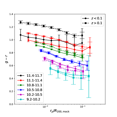
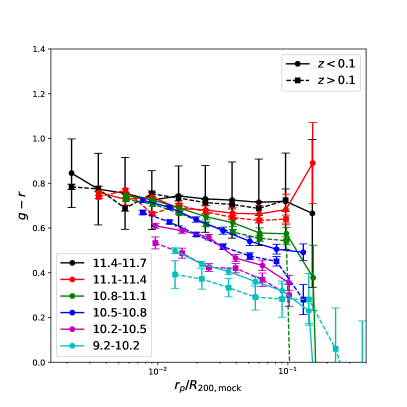
Figure 17: $g-r$ color profiles before (left) and after (right) PSF and $K$-corrections, and for ICGs grouped in a few different stellar mass bins (see the legend).

In the left plot of Figure 17, we show the color profiles for ICGs in two redshift bins without including PSF and $K$-corrections. For ICGs more massive than $\log_{10}M_{\ast}/\mathrm{M}_{\odot}>10.8$, the higher redshift subsample tends to have redder colors, which is due to the ignorance of $K$-correction. Massive galaxies are mostly red, and their passive evolution with redshift is weak, while the prominent 4000Å break feature of massive galaxies due to absorption shifts to redder bands with the increase in redshift, resulting in prominently redder colors. For less massive ICGs, they are dominated by star-forming galaxies and have less or no prominent 4000Å break features. We can see the subsample at higher redshifts tends to have bluer colors. This is due to the selection bias caused by the survey flux limit. At a fixed stellar mass, blue star-forming galaxies have smaller stellar-mass-to-light ratios, and are brighter. Thus for a fixed flux limit at a given redshift, more small blue star-forming galaxies can be observed. Hence bluer galaxies tend to be observed in the higher redshift bin.

In the right plot of Figure 17, PSF and $K$-corrections have been included. After $K$-corrections, massive ICGs at different redshifts now have very similar $g-r$ color profiles ($\log_{10}M_{\ast}/\mathrm{M}_{\odot}>11.1$). This proves that our empirical $K$-correction works reasonably well. Besides, for ICGs less massive than $\log_{10}M_{\ast}/\mathrm{M}_{\odot}\sim 11.1$, the higher redshift subsamples all tend to have bluer colors, which are more prominent for smaller ICGs and also more significant than the left plot. This is because, after eliminating the effect of ignoring $K$-corrections, the selection bias of a given flux limit, as explained above, becomes more prominent, which cannot be eliminated after applying $K$-corrections.

References

- Abazajian et al. (2009) Abazajian, K. N., Adelman-McCarthy, J. K., Agüeros, M. A., et al. 2009, ApJS, 182, 543, doi: 10.1088/0067-0049/182/2/543
- Aihara et al. (2018a) Aihara, H., Arimoto, N., Armstrong, R., et al. 2018a, PASJ, 70, S4, doi: 10.1093/pasj/psx066
- Aihara et al. (2018b) Aihara, H., Armstrong, R., Bickerton, S., et al. 2018b, PASJ, 70, S8, doi: 10.1093/pasj/psx081
- Aihara et al. (2019) Aihara, H., AlSayyad, Y., Ando, M., et al. 2019, PASJ, 71, 114, doi: 10.1093/pasj/psz103
- Astropy Collaboration et al. (2013) Astropy Collaboration, Robitaille, T. P., Tollerud, E. J., et al. 2013, A&A, 558, A33, doi: 10.1051/0004-6361/201322068
- Axelrod et al. (2010) Axelrod, T., Kantor, J., Lupton, R. H., & Pierfederici, F. 2010, in Proc. SPIE, Vol. 7740, Software and Cyberinfrastructure for Astronomy, 774015, doi: 10.1117/12.857297
- Bernstein & Jarvis (2002) Bernstein, G. M., & Jarvis, M. 2002, AJ, 123, 583, doi: 10.1086/338085
- Bertin & Arnouts (1996) Bertin, E., & Arnouts, S. 1996, A&AS, 117, 393, doi: 10.1051/aas:1996164
- Blanton & Roweis (2007) Blanton, M. R., & Roweis, S. 2007, AJ, 133, 734, doi: 10.1086/510127
- Blanton et al. (2005) Blanton, M. R., Schlegel, D. J., Strauss, M. A., et al. 2005, AJ, 129, 2562, doi: 10.1086/429803
- Bosch et al. (2018) Bosch, J., Armstrong, R., Bickerton, S., et al. 2018, PASJ, 70, S5, doi: 10.1093/pasj/psx080
- Boylan-Kolchin et al. (2011) Boylan-Kolchin, M., Bullock, J. S., & Kaplinghat, M. 2011, MNRAS, 415, L40, doi: 10.1111/j.1745-3933.2011.01074.x
- Bullock & Johnston (2005) Bullock, J. S., & Johnston, K. V. 2005, ApJ, 635, 931, doi: 10.1086/497422
- Bundy et al. (2010) Bundy, K., Scarlata, C., Carollo, C. M., et al. 2010, ApJ, 719, 1969, doi: 10.1088/0004-637X/719/2/1969
- Carlsten et al. (2021) Carlsten, S. G., Greene, J. E., Peter, A. H. G., Beaton, R. L., & Greco, J. P. 2021, ApJ, 908, 109, doi: 10.3847/1538-4357/abd039
- Cautun et al. (2015a) Cautun, M., Bose, S., Frenk, C. S., et al. 2015a, MNRAS, 452, 3838, doi: 10.1093/mnras/stv1557
- Cautun et al. (2015b) Cautun, M., Wang, W., Frenk, C. S., & Sawala, T. 2015b, MNRAS, 449, 2576, doi: 10.1093/mnras/stv490
- Chen et al. (2006) Chen, J., Kravtsov, A. V., Prada, F., et al. 2006, ApJ, 647, 86, doi: 10.1086/504462
- Cooper et al. (2013) Cooper, A. P., D’Souza, R., Kauffmann, G., et al. 2013, MNRAS, 434, 3348, doi: 10.1093/mnras/stt1245
- Cooper et al. (2015) Cooper, A. P., Gao, L., Guo, Q., et al. 2015, MNRAS, 451, 2703, doi: 10.1093/mnras/stv1042
- Cooper et al. (2010) Cooper, A. P., Cole, S., Frenk, C. S., et al. 2010, MNRAS, 406, 744, doi: 10.1111/j.1365-2966.2010.16740.x
- Cui et al. (2014) Cui, W., Murante, G., Monaco, P., et al. 2014, MNRAS, 437, 816, doi: 10.1093/mnras/stt1940
- Cunha et al. (2009) Cunha, C. E., Lima, M., Oyaizu, H., Frieman, J., & Lin, H. 2009, MNRAS, 396, 2379, doi: 10.1111/j.1365-2966.2009.14908.x
- de Jong (2008) de Jong, R. S. 2008, MNRAS, 388, 1521, doi: 10.1111/j.1365-2966.2008.13505.x
- D’Souza et al. (2014) D’Souza, R., Kauffman, G., Wang, J., & Vegetti, S. 2014, MNRAS, 443, 1433, doi: 10.1093/mnras/stu1194
- D’Souza et al. (2015) D’Souza, R., Vegetti, S., & Kauffmann, G. 2015, MNRAS, 454, 4027, doi: 10.1093/mnras/stv2234
- Fong & Han (2021) Fong, M., & Han, J. 2021, MNRAS, doi: 10.1093/mnras/stab259
- Font et al. (2011) Font, A. S., Benson, A. J., Bower, R. G., et al. 2011, MNRAS, 417, 1260, doi: 10.1111/j.1365-2966.2011.19339.x
- Foreman-Mackey et al. (2013) Foreman-Mackey, D., Hogg, D. W., Lang, D., & Goodman, J. 2013, PASP, 125, 306, doi: 10.1086/670067
- Furnell et al. (2021) Furnell, K. E., Collins, C. A., Kelvin, L. S., et al. 2021, MNRAS, 502, 2419, doi: 10.1093/mnras/stab065
- Furusawa et al. (2018) Furusawa, H., Koike, M., Takata, T., et al. 2018, PASJ, 70, S3, doi: 10.1093/pasj/psx079
- Garcia et al. (2020) Garcia, R., Rozo, E., Becker, M. R., & More, S. 2020, arXiv e-prints, arXiv:2006.12751. https://arxiv.org/abs/2006.12751
- Gonzalez et al. (2013) Gonzalez, A. H., Sivanandam, S., Zabludoff, A. I., & Zaritsky, D. 2013, ApJ, 778, 14, doi: 10.1088/0004-637X/778/1/14
- Guo et al. (2011a) Guo, Q., Cole, S., Eke, V., & Frenk, C. 2011a, MNRAS, 417, 370, doi: 10.1111/j.1365-2966.2011.19270.x
- Guo et al. (2012) —. 2012, MNRAS, 427, 428, doi: 10.1111/j.1365-2966.2012.21882.x
- Guo et al. (2015) Guo, Q., Cooper, A. P., Frenk, C., Helly, J., & Hellwing, W. A. 2015, MNRAS, 454, 550, doi: 10.1093/mnras/stv1938
- Guo et al. (2010) Guo, Q., White, S., Li, C., & Boylan-Kolchin, M. 2010, MNRAS, 404, 1111, doi: 10.1111/j.1365-2966.2010.16341.x
- Guo et al. (2011b) Guo, Q., White, S., Boylan-Kolchin, M., et al. 2011b, MNRAS, 413, 101, doi: 10.1111/j.1365-2966.2010.18114.x
- Han et al. (2019) Han, J., Li, Y., Jing, Y., et al. 2019, MNRAS, 482, 1900, doi: 10.1093/mnras/sty2822
- Han et al. (2015a) Han, J., Eke, V. R., Frenk, C. S., et al. 2015a, MNRAS, 446, 1356, doi: 10.1093/mnras/stu2178
- Han et al. (2015b) —. 2015b, MNRAS, 446, 1356, doi: 10.1093/mnras/stu2178
- Hao et al. (2019) Hao, C.-N., Shi, Y., Chen, Y., et al. 2019, ApJ, 883, L36, doi: 10.3847/2041-8213/ab42e5
- Harmsen et al. (2017) Harmsen, B., Monachesi, A., Bell, E. F., et al. 2017, MNRAS, 466, 1491, doi: 10.1093/mnras/stw2992
- Hayashi & White (2008) Hayashi, E., & White, S. D. M. 2008, MNRAS, 388, 2, doi: 10.1111/j.1365-2966.2008.13371.x
- He et al. (2013) He, Y. Q., Xia, X. Y., Hao, C. N., et al. 2013, ApJ, 773, 37, doi: 10.1088/0004-637X/773/1/37
- Hirata & Seljak (2003) Hirata, C., & Seljak, U. 2003, MNRAS, 343, 459, doi: 10.1046/j.1365-8711.2003.06683.x
- Huang et al. (2018) Huang, S., Leauthaud, A., Greene, J. E., et al. 2018, MNRAS, 475, 3348, doi: 10.1093/mnras/stx3200
- Hudson et al. (2015) Hudson, M. J., Gillis, B. R., Coupon, J., et al. 2015, MNRAS, 447, 298, doi: 10.1093/mnras/stu2367
- James & Roos (1975) James, F., & Roos, M. 1975, Computer Physics Communications, 10, 343, doi: 10.1016/0010-4655(75)90039-9
- Jee & Tyson (2011) Jee, M. J., & Tyson, J. A. 2011, PASP, 123, 596, doi: 10.1086/660137
- Jiang et al. (2012) Jiang, C. Y., Jing, Y. P., & Li, C. 2012, ApJ, 760, 16, doi: 10.1088/0004-637X/760/1/16
- Jurić et al. (2017) Jurić, M., Kantor, J., Lim, K.-T., et al. 2017, in Astronomical Society of the Pacific Conference Series, Vol. 512, Astronomical Data Analysis Software and Systems XXV, ed. N. P. F. Lorente, K. Shortridge, & R. Wayth, 279. https://arxiv.org/abs/1512.07914
- Karademir et al. (2018) Karademir, G. S., Remus, R.-S., Burkert, A., et al. 2018, ArXiv e-prints. https://arxiv.org/abs/1808.10454
- Kawanomoto et al. (2018) Kawanomoto, S., Uraguchi, F., Komiyama, Y., et al. 2018, PASJ, 70, 66, doi: 10.1093/pasj/psy056
- Kawinwanichakij et al. (2014) Kawinwanichakij, L., Papovich, C., Quadri, R. F., et al. 2014, ApJ, 792, 103, doi: 10.1088/0004-637X/792/2/103
- Keller (2021) Keller, B. W. 2021, arXiv e-prints, arXiv:2103.09833. https://arxiv.org/abs/2103.09833
- Klypin et al. (1999) Klypin, A., Kravtsov, A. V., Valenzuela, O., & Prada, F. 1999, ApJ, 522, 82, doi: 10.1086/307643
- Koekemoer et al. (2007) Koekemoer, A. M., Aussel, H., Calzetti, D., et al. 2007, ApJS, 172, 196, doi: 10.1086/520086
- Komiyama et al. (2018) Komiyama, Y., Obuchi, Y., Nakaya, H., et al. 2018, PASJ, 70, S2, doi: 10.1093/pasj/psx069
- Koposov et al. (2009) Koposov, S. E., Yoo, J., Rix, H.-W., et al. 2009, ApJ, 696, 2179, doi: 10.1088/0004-637X/696/2/2179
- Lackner et al. (2012) Lackner, C. N., Cen, R., Ostriker, J. P., & Joung, M. R. 2012, MNRAS, 425, 641, doi: 10.1111/j.1365-2966.2012.21525.x
- Lan et al. (2016) Lan, T.-W., Ménard, B., & Mo, H. 2016, MNRAS, 459, 3998, doi: 10.1093/mnras/stw898
- Lares et al. (2011) Lares, M., Lambas, D. G., & Domínguez, M. J. 2011, AJ, 142, 13, doi: 10.1088/0004-6256/142/1/13
- Leauthaud et al. (2012) Leauthaud, A., Tinker, J., Bundy, K., et al. 2012, ApJ, 744, 159, doi: 10.1088/0004-637X/744/2/159
- Lorrimer et al. (1994) Lorrimer, S. J., Frenk, C. S., Smith, R. M., White, S. D. M., & Zaritsky, D. 1994, MNRAS, 269, 696, doi: 10.1093/mnras/269.3.696
- Man et al. (2019) Man, Z.-Y., Peng, Y.-J., Shi, J.-J., et al. 2019, ApJ, 881, 74, doi: 10.3847/1538-4357/ab2ece
- Mandelbaum et al. (2005) Mandelbaum, R., Tasitsiomi, A., Seljak, U., Kravtsov, A. V., & Wechsler, R. H. 2005, MNRAS, 362, 1451, doi: 10.1111/j.1365-2966.2005.09417.x
- Mandelbaum et al. (2016) Mandelbaum, R., Wang, W., Zu, Y., et al. 2016, MNRAS, 457, 3200, doi: 10.1093/mnras/stw188
- Mandelbaum et al. (2018a) Mandelbaum, R., Lanusse, F., Leauthaud, A., et al. 2018a, MNRAS, 481, 3170, doi: 10.1093/mnras/sty2420
- Mandelbaum et al. (2018b) Mandelbaum, R., Miyatake, H., Hamana, T., et al. 2018b, PASJ, 70, S25, doi: 10.1093/pasj/psx130
- Mao et al. (2021) Mao, Y.-Y., Geha, M., Wechsler, R. H., et al. 2021, ApJ, 907, 85, doi: 10.3847/1538-4357/abce58
- Merritt et al. (2020) Merritt, A., Pillepich, A., van Dokkum, P., et al. 2020, MNRAS, 495, 4570, doi: 10.1093/mnras/staa1164
- Merritt et al. (2016) Merritt, A., van Dokkum, P., Abraham, R., & Zhang, J. 2016, ApJ, 830, 62, doi: 10.3847/0004-637X/830/2/62
- Miyazaki et al. (2012) Miyazaki, S., Komiyama, Y., Nakaya, H., et al. 2012, in Proc. SPIE, Vol. 8446, Ground-based and Airborne Instrumentation for Astronomy IV, 84460Z, doi: 10.1117/12.926844
- Miyazaki et al. (2018) Miyazaki, S., Komiyama, Y., Kawanomoto, S., et al. 2018, PASJ, 70, S1, doi: 10.1093/pasj/psx063
- Moore et al. (1999) Moore, B., Ghigna, S., Governato, F., et al. 1999, ApJ, 524, L19, doi: 10.1086/312287
- Moster et al. (2013) Moster, B. P., Naab, T., & White, S. D. M. 2013, MNRAS, 428, 3121, doi: 10.1093/mnras/sts261
- Moster et al. (2010) Moster, B. P., Somerville, R. S., Maulbetsch, C., et al. 2010, ApJ, 710, 903, doi: 10.1088/0004-637X/710/2/903
- Nakajima et al. (2012) Nakajima, R., Mandelbaum, R., Seljak, U., et al. 2012, MNRAS, 420, 3240, doi: 10.1111/j.1365-2966.2011.20249.x
- Nierenberg et al. (2013) Nierenberg, A. M., Treu, T., Menci, N., Lu, Y., & Wang, W. 2013, ApJ, 772, 146, doi: 10.1088/0004-637X/772/2/146
- Nishizawa et al. (2020) Nishizawa, A. J., Hsieh, B.-C., Tanaka, M., & Takata, T. 2020, arXiv e-prints, arXiv:2003.01511. https://arxiv.org/abs/2003.01511
- Oh et al. (2017) Oh, S., Greene, J. E., & Lackner, C. N. 2017, ApJ, 836, 115, doi: 10.3847/1538-4357/836/1/115
- Oser et al. (2010) Oser, L., Ostriker, J. P., Naab, T., Johansson, P. H., & Burkert, A. 2010, ApJ, 725, 2312, doi: 10.1088/0004-637X/725/2/2312
- Peng et al. (2012) Peng, Y.-j., Lilly, S. J., Renzini, A., & Carollo, M. 2012, ApJ, 757, 4, doi: 10.1088/0004-637X/757/1/4
- Phillipps & Shanks (1987) Phillipps, S., & Shanks, T. 1987, MNRAS, 229, 621, doi: 10.1093/mnras/229.4.621
- Pillepich et al. (2014) Pillepich, A., Vogelsberger, M., Deason, A., et al. 2014, MNRAS, 444, 237, doi: 10.1093/mnras/stu1408
- Planck Collaboration et al. (2014) Planck Collaboration, Ade, P. A. R., Aghanim, N., et al. 2014, A&A, 571, A16, doi: 10.1051/0004-6361/201321591
- Puchwein et al. (2010) Puchwein, E., Springel, V., Sijacki, D., & Dolag, K. 2010, MNRAS, 406, 936, doi: 10.1111/j.1365-2966.2010.16786.x
- Purcell et al. (2007) Purcell, C. W., Bullock, J. S., & Zentner, A. R. 2007, ApJ, 666, 20, doi: 10.1086/519787
- Rodriguez-Gomez et al. (2016) Rodriguez-Gomez, V., Pillepich, A., Sales, L. V., et al. 2016, MNRAS, 458, 2371, doi: 10.1093/mnras/stw456
- Rodríguez-Puebla et al. (2015) Rodríguez-Puebla, A., Avila-Reese, V., Yang, X., et al. 2015, ApJ, 799, 130, doi: 10.1088/0004-637X/799/2/130
- Sales & Lambas (2005) Sales, L., & Lambas, D. G. 2005, MNRAS, 356, 1045, doi: 10.1111/j.1365-2966.2004.08518.x
- Sales et al. (2013) Sales, L. V., Wang, W., White, S. D. M., & Navarro, J. F. 2013, MNRAS, 428, 573, doi: 10.1093/mnras/sts054
- Szomoru et al. (2010) Szomoru, D., Franx, M., van Dokkum, P. G., et al. 2010, ApJ, 714, L244, doi: 10.1088/2041-8205/714/2/L244
- Tal & van Dokkum (2011) Tal, T., & van Dokkum, P. G. 2011, ApJ, 731, 89, doi: 10.1088/0004-637X/731/2/89
- Tal et al. (2012) Tal, T., Wake, D. A., & van Dokkum, P. G. 2012, ApJ, 751, L5, doi: 10.1088/2041-8205/751/1/L5
- Tinker et al. (2019) Tinker, J. L., Cao, J., Alpaslan, M., et al. 2019, arXiv e-prints, arXiv:1911.04507. https://arxiv.org/abs/1911.04507
- Tollerud et al. (2011) Tollerud, E. J., Boylan-Kolchin, M., Barton, E. J., Bullock, J. S., & Trinh, C. Q. 2011, ApJ, 738, 102, doi: 10.1088/0004-637X/738/1/102
- Vader & Sandage (1991) Vader, J. P., & Sandage, A. 1991, ApJ, 379, L1, doi: 10.1086/186140
- Wang et al. (2018) Wang, C., Li, R., Gao, L., et al. 2018, MNRAS, 475, 4020, doi: 10.1093/mnras/sty073
- Wang et al. (2013a) Wang, L., De Lucia, G., & Weinmann, S. M. 2013a, MNRAS, 431, 600, doi: 10.1093/mnras/stt188
- Wang & Jing (2010) Wang, L., & Jing, Y. P. 2010, MNRAS, 402, 1796, doi: 10.1111/j.1365-2966.2009.16007.x
- Wang et al. (2013b) Wang, L., Farrah, D., Oliver, S. J., et al. 2013b, MNRAS, 431, 648, doi: 10.1093/mnras/stt190
- Wang et al. (2011) Wang, W., Jing, Y. P., Li, C., Okumura, T., & Han, J. 2011, ApJ, 734, 88, doi: 10.1088/0004-637X/734/2/88
- Wang et al. (2014) Wang, W., Sales, L. V., Henriques, B. M. B., & White, S. D. M. 2014, MNRAS, 442, 1363, doi: 10.1093/mnras/stu988
- Wang & White (2012) Wang, W., & White, S. D. M. 2012, MNRAS, 424, 2574, doi: 10.1111/j.1365-2966.2012.21256.x
- Wang et al. (2019) Wang, W., Han, J., Sonnenfeld, A., et al. 2019, MNRAS, 487, 1580, doi: 10.1093/mnras/stz1339
- Wang et al. (2021) Wang, W., Takada, M., Li, X., et al. 2021, MNRAS, 500, 3776, doi: 10.1093/mnras/staa3495
- Westra et al. (2010) Westra, E., Geller, M. J., Kurtz, M. J., Fabricant, D. G., & Dell’Antonio, I. 2010, PASP, 122, 1258, doi: 10.1086/657452
- White & Rees (1978) White, S. D. M., & Rees, M. J. 1978, MNRAS, 183, 341, doi: 10.1093/mnras/183.3.341
- Wright & Brainerd (2000) Wright, C. O., & Brainerd, T. G. 2000, ApJ, 534, 34, doi: 10.1086/308744
- Yang et al. (2009) Yang, X., Mo, H. J., & van den Bosch, F. C. 2009, ApJ, 693, 830, doi: 10.1088/0004-637X/693/1/830
- Yang et al. (2012) Yang, X., Mo, H. J., van den Bosch, F. C., Zhang, Y., & Han, J. 2012, ApJ, 752, 41, doi: 10.1088/0004-637X/752/1/41
- Zhang et al. (2019) Zhang, Y., Yanny, B., Palmese, A., et al. 2019, ApJ, 874, 165, doi: 10.3847/1538-4357/ab0dfd
- Zibetti et al. (2004) Zibetti, S., White, S. D. M., & Brinkmann, J. 2004, MNRAS, 347, 556, doi: 10.1111/j.1365-2966.2004.07235.x
- Zibetti et al. (2005) Zibetti, S., White, S. D. M., Schneider, D. P., & Brinkmann, J. 2005, MNRAS, 358, 949, doi: 10.1111/j.1365-2966.2005.08817.x