18329 \lmcsheadingLABEL:LastPageJul. 28, 2021Sep. 07, 2022
A preliminary version of this work was published in the accompanying paper for the invited talk given by Thomas Colcombet at the International Conference on Foundations of Software Science and Computation Structures (FoSSaCS) [CF19], see also the corresponding technical reports [CF18] and [Fij18]. The applications to mean payoff games (Section 7) was published in the International Symposium on Mathematical Foundations of Computer Science (MFCS) [FGO20]. The applications to disjunctions of mean payoff and parity games (Section 8) and disjunctions of mean payoff games (Section 9) are unpublished.
The Theory of Universal Graphs
for Infinite Duration Games
Abstract.
We introduce the notion of universal graphs as a tool for constructing algorithms solving games of infinite duration such as parity games and mean payoff games. In the first part we develop the theory of universal graphs, with two goals: showing an equivalence and normalisation result between different recently introduced related models, and constructing generic value iteration algorithms for any positionally determined objective. In the second part we give four applications: to parity games, to mean payoff games, to a disjunction between a parity and a mean payoff objective, and to disjunctions of several mean payoff objectives. For each of these four cases we construct algorithms achieving or improving over the best known time and space complexity.
Key words and phrases:
Games on graphs, parity games, mean payoff games, universal graphs1. Introduction
Games of infinite duration are a widely studied model in several fields of Computer Science including Program Verification, Model checking, Automata Theory, Logic, Finite Model Theory, and Database Theory: the interactions between the players can model a range of (non-terminating) systems and are therefore used for analysing, verifying, and synthesising them. There is a wide range of game models: in this paper we consider two player zero sum deterministic (as opposed to stochastic) games with perfect information. Two of the most important open problems in this field concern parity games and mean payoff games: in both cases the complexity of solving them is in NP and in coNP, but not known to be in polynomial time. This complexity status was once shared with primality testing, linear programming, and other famous problems, which all turned out to be solvable in polynomial time. Yet although both problems have attracted a lot of attention over the past three decades, they remain widely open and exciting research directions. This paper introduces the combinatorial notion of universal graphs and constructs conceptually simple algorithms achieving state of the art time and space complexity for both parity and mean payoff games, and beyond. In order to motivate the introduction of universal graphs, let us revisit the recent developments on parity games.
Parity games are a central model in the study of logic and automata over infinite trees and for their tight relationship with model-checking games for the modal -calculus. The breakthrough result of Calude, Jain, Khoussainov, Li, and Stephan [CJK+17] was to construct a quasipolynomial time algorithm for solving parity games. Following decades of exponential and subexponential algorithms, this very surprising result triggered further research: soon after further quasipolynomial time algorithms were constructed reporting almost the same complexity. Let us classify them in two families; we will motivate this classification in the next paragraphs.
-
•
The first family of algorithms includes the original algorithm by Calude, Jain, Khoussainov, Li, and Stephan [CJK+17] (see also [FJS+17] for a presentation of the algorithm as value iteration), then the succinct progress measure lifting algorithm by Jurdziński and Lazić [JL17], and the register games algorithm by Lehtinen [Leh18] (see also the journal version [LB20]).
-
•
The second family of algorithms is so-called McNaughton Zielonka-type algorithms, inspired by the exponential time algorithm by Zielonka [Zie98] specialising an algorithm due to McNaughton [McN93]. The first quasipolynomial time algorithm is due to Parys [Par19]. Its complexity was later improved by Lehtinen, Schewe, and Wojtczak [LSW19]. Recently Jurdziński and Morvan [JM20] constructed a universal attractor decomposition algorithm encompassing all three algorithms, which was then refined and further studied in [JMOT20].
Separating automata have been introduced by Bojańczyk and Czerwiński [BC18] in an effort to understand the first quasipolynomial time algorithm: they have extracted from the algorithm the construction of a separating automaton and presented the original algorithm as solving a safety game obtained as the product of the original game by the separating automaton. Later Czerwiński, Daviaud, Fijalkow, Jurdziński, Lazić, and Parys [CDF+18] showed that the other two algorithms also induce separating automata. Separating automata are deterministic; we refer to Subsection 6.4 for a more in-depth discussion on the use of non-determinism.
Universal trees have been defined by Fijalkow [Fij18] (superseded by [CDF+18]) to rephrase the second quasipolynomial time algorithm [JL17], constructing a family of value iteration algorithms parametrised by the choice of a universal tree. Within this family the algorithm [JL17] is optimal: the universal tree (implicitly) constructed in [JL17] matches (up to a polynomial factor) the lower bounds offered in [Fij18]. The main contribution of [CDF+18] is to show that any separating automaton contains a universal tree in its set of states; in other words, the three algorithms in the first family induce three (different) constructions of universal trees.
The generic algorithm constructed in [JM20] is parametrised by the choice of two universal trees (one of each player), and it is argued that choosing appropriate pairs of universal trees yields the algorithms from [Zie98, Par19, LSW19].
Ubiquity of universal trees. In summary, all quasipolynomial time algorithms for parity games (and some exponential ones) fall in one of two families, and both are based on the combinatorial notion of universal trees. This has a number of consequences:
-
•
simplicity: all algorithms are instances of one of two generic algorithms,
-
•
combinatorial abstraction: algorithms have been reduced to a purely combinatorial notion on trees which is easier to study and captures the combinatorial contents and complexity of the algorithms,
-
•
lower bounds: the lower bounds on universal trees imply a complexity barrier applying to both families of algorithms, hence to all known quasipolynomial time algorithms.
Beyond parity games. There are a number of other objectives of interest, the most prominent one being mean payoff. We introduce universal graphs for any objective which is positionally determined for at least one of the two players (with some additional technical assumptions, see Subsection 2.3) with the following goals: constructing generic algorithms, reducing the construction of algorithms to the combinatorial understanding of universal graphs, and offering lower bounds to argue about the optimality of the algorithms within this framework. As we shall see, when the objective corresponds to parity games, universal graphs instantiate as universal trees.
Our contributions and outline. The first part of the paper is to develop the theory of universal graphs.
After the mandatory preliminaries in Section 2, we start in Section 3 by constructing a generic algorithm for solving games by reduction to safety games. We present three sufficient conditions for this algorithm to be correct: using a separating automaton, using a good-for-small-games automaton, or using a universal graph. We give in Section 4 the main technical result of the theory of universal graphs: it is a normalisation result through a saturation process showing the equivalence of the three models. A first consequence of this normalisation is an efficient implementation of the generic algorithm defined in Section 3 as a value iteration algorithm, constructed in Section 5.
The second part of the paper is to give four applications of the universal graph approach: for four classes of objectives, we construct universal graphs and derive algorithms for solving the corresponding games. Since the complexity of the algorithm is proportional to the size of the universal graph, our goal is to construct as small as possible universal graphs. In all four cases our algorithms achieve the best known time and space complexity for solving the corresponding games, even significantly improving the state of the art in one case. Along the way we will explain that many existing algorithms are actually instances of our framework, meaning are solving implicitly or explicitly a product game for some universal graph.
In these four applications we use two different approaches for studying universal graphs:
-
•
Both for parity and mean payoff objectives, we first study the properties of saturated universal graphs, find a combinatorial characterisation: using trees for parity objectives (Section 6) and subsets of the integers for mean payoff objectives (Section 7). Using these combinatorial characterisations we prove upper and lower bounds on the size of universal graphs: the upper bounds induce algorithms for solving the corresponding games, and the lower bounds imply that the algorithms we construct are optimal within this class of algorithms.
-
•
Both for disjunctions of a parity and a mean payoff objective, and for disjunctions of several mean payoff objectives111Although this distinction is irrelevant for mean payoff games, it matters whether one uses the or semantics when considering their disjunctions (see [VCD+15]). Here, we only consider semantics, which is algorithmically tractable., we investigate how to combine existing universal graphs for each objective into universal graphs for their disjunctions. We provide some general results towards this goal, in particular a reduction to strongly connected graphs in Section 9. For disjunctions of a parity and a mean payoff objective (Section 8) it is more convenient to reason with separating automata, which thanks to our general equivalence theorem (Theorem 9) is equivalent with respect to size, our main concern for algorithmic applications.
2. Preliminaries
We write for the interval , and use parentheses to exclude extremal values, so for instance is . We let denote a set of colours and write for finite sequences of colours (also called finite words), for finite non-empty sequences, and for infinite sequences (also called infinite words). The empty word is .
2.1. Graphs are safety automata and safety automata are graphs
Graphs
We consider edge labelled directed graphs: a graph is given by a (finite) set of vertices and a (finite) set of edges, with a set of colours, so we write . An edge is from the vertex to the vertex and is labelled by the colour . The size of a graph is its number of vertices. A vertex for which there exists no outgoing edges is called a sink.
Paths
A path is a (finite or infinite) sequence
where for all we have . If it is finite, that is, , we call the length of , and use to denote the last vertex . The length of an infinite path is . We say that starts from or is a path from , and in the case where is finite we say that is a path ending in or simply a path to . We say that is reachable from if there exists a path from to . We let denote the prefix of ending in , meaning . A cycle is a path from a vertex to itself of length at least one.
We use and to denote respectively the sets of finite paths of , infinite paths of , and their union. We sometimes drop when it is clear from context. For we also use and to refer to the sets of paths starting from . We use to denote the (finite or infinite) sequence of colours induced by .
Objectives
An objective is a set of infinite sequences of colours. We say that a sequence of colours belonging to satisfies , and extend this terminology to infinite paths with .
[Graphs satisfying an objective] Let be an objective and a graph. We say that satisfies if all infinite paths in satisfy .
Safety automata
A safety automaton over the alphabet is given by a finite set of states and a transition function , so we write . Since we are only considering safety automata in this paper, we omit the adjective safety and simply speak of an automaton. A first very important remark is that a (safety) automaton is simply a graph; this point of view will be very important and fruitful in this paper.
An automaton recognises the language of infinite words defined as follows:
The class of deterministic automata has two additional properties: the automaton has a designated initial state , and for any state and colour there is at most one transition of the form in . In that case we define such that is the unique where if it is defined. We extend to sequences of colours by the formulas and . The language recognised by a deterministic automaton is defined by . Note that if is a finite prefix of a word in , then is well defined.
Following our convention to identify non-deterministic automata and graphs, we say that satisfies if .
2.2. Games
Arenas
An arena is given by a graph together with a partition of its set of vertices describing which player controls each vertex. We represent vertices controlled by Eve with circles and those controlled by Adam with squares.
Games
A game is given by an arena and an objective . We often let denote a game, and use for the underlying graph. The size of is defined to be the size of the underlying graph . It is played as follows. A token is initially placed on some vertex , and the player who controls this vertex pushes the token along an edge, reaching a new vertex; the player who controls this new vertex takes over, and this interaction goes on, either forever and describing an infinite path, or until reaching a sink.
We say that a path is winning222We always take the point of view of Eve, so winning means winning for Eve, and similarly a strategy is a strategy for Eve. if it is infinite and satisfies , or finite and ends in a sink controlled by Adam. The definition of a winning path includes the following usual convention: if a player cannot move they lose, in other words sinks controlled by Adam are winning (for Eve) and sinks controlled by Eve are losing.
We extend the notations and Path to games by considering the underlying graph.
Strategies
A strategy in is a partial map such that is an outgoing edge of when it is defined. We say that a path is consistent with if for all , if then is defined over and . A consistent path with is maximal if it is not the strict prefix of a consistent path with (in particular infinite consistent paths are maximal).
A strategy is winning from if all maximal paths consistent with are winning. Note that in particular, if a finite path is consistent with a winning strategy and ends in a vertex which belongs to Eve, then is defined over . We say that is a winning vertex of or that Eve wins from in if there exists a winning strategy from , and let denote the set of winning vertices.
Positional strategies
Positional strategies make decisions only considering the current vertex. Such a strategy is given by . A positional strategy induces a strategy from any vertex by setting when .
[Positionally determined objectives] We say that an objective is positionally determined if for every game with objective and vertex , if then there exists a positional winning strategy from .
Given a game , a vertex , and a positional strategy we let denote the graph obtained by restricting to vertices reachable from by playing and to the moves prescribed by . Formally, the set of vertices and edges is
[Prefix independent objectives] We say that an objective is prefix independent if for all and , we have if and only if .
Fact 1.
Let be a prefix independent objective, a game, a vertex, and a positional strategy. Then is winning from if and only if the graph satisfies and does not contain any sink controlled by Eve.
Safety games
The safety objective is defined over the set of colours by : in words, all infinite paths are winning, so losing for Eve can only result from reaching a sink that she controls. Since there is a unique colour, when manipulating safety games we ignore the colour component for edges. Note that in safety games, strategies can equivalently be defined as maps to (and not ): only the target of an edge matters when the source is fixed, since there is a unique colour. We sometimes use this abuse of notations for the sake of simplicity and conciseness.
The following result is folklore, we refer to Section 5 for more details on the algorithm. The statement uses the classical RAM model with word size .
Theorem 2.
There exists an algorithm computing the set of winning vertices of a safety game running in time .
2.3. Assumptions on objectives
[Neutral letter] Let an objective and . For we let denote the projection of on , that is, the finite or infinite word obtained by removing all occurrences of in . We say that is a neutral letter if for all , if is finite then , and if is infinite, then if and only if .
In this paper, we will prove results applying to general objectives satisfying three assumptions:
-
•
is positionally determined,
-
•
is prefix independent,
-
•
has a neutral letter.
The first assumption is at the heart of the approach; the other two are here rather for technical convenience. In fact, it is not known whether there are positional objectives for which artificially adding a neutral letter breaks positionality [Kop06]. Regarding prefix independence, we believe that our techniques can be adapted by fixing an initial vertex (both in the games under consideration and in the universal graph), but chose not to pursue this path for the sake of simplicity and convenience.
3. Reductions to safety games
This section describes different ways to reduce solving a game with a positionally determined objective to solving a (larger) equivalent safety game, using a product construction with an automaton (or equivalently, a graph). In this section we introduce the concepts needed to prove the following theorem.
Theorem 3.
Let , a positionally determined objective, a game of size with objective , and be either an -separating automaton (defined in Subsection 3.2) an -GFSG automaton (defined in Subsection 3.3) or an -universal graph (defined in Subsection 3.4). Then the winning region in can be computed333In the RAM model with word size . in time .
In all three cases, this is obtained by reducing to the safety game , and then applying Theorem 2. The three notions (separating automata, GFSG automata, and universal graphs) are sufficient conditions for the two games and to be equivalent. We start by describing the product construction .
3.1. Product construction
Let be an automaton and a game with objective . We define the chained game as the safety game with vertices and edges given by
In words, from , the player whom belongs to chooses an edge , and the game progresses to . Then Eve chooses a transition in , and the game continues from . Intuitively, we simulate playing in , but additionally Eve has to simultaneously follow a path in which reads the same colours. Note that the obtained game is a safety game: Eve wins if she can play forever or end up in a sink controlled by Adam.
Lemma 4.
Let be an objective, a game with objective , an automaton, and . If satisfies and is such that Eve wins from in , then Eve wins from in .
Intuitively, if Eve can play forever in , and all paths in are labelled by sequences which belong to , then Eve can use the same strategy in and obtain a path satisfying . The formal proof requires some technical care for transferring the strategy from to .
Proof 3.1.
Let be a winning strategy from in . We construct a strategy , from in which simulates in the following sense, which we call the simulation property:
for any path in which is consistent with ,
there exists a sequence of states such that ,
with for , is a path in consistent with .
We define over finite paths with by induction over , so that the simulation property holds. For there is nothing to prove since is a path in consistent with . Let be a path in consistent with and , we want to define . Thanks to the simulation property there exists such that is a path in consistent with . Then , so since it is winning, is defined over , let us write with . We set .
To conclude the definition of we need to show that the simulation property extends to paths of length . Let be consistent with . We apply the simulation property to to construct such that is a path in consistent with . Let us consider with , we claim that is consistent with . Indeed, if , there is nothing to prove, and if , this holds by construction: since we have . Now so is defined over , and we let . Then is consistent with . This concludes the inductive proof of the simulation property together with the definition of .
We now prove that is a winning strategy from . Let be a maximal consistent path with , and let be the corresponding path in consistent with . Let us first assume that is finite, and let . If , then by construction is defined over , so the path , where is consistent with , contradicting maximality of . If however , then by maximality of , must be a sink, hence is winning. Now if is infinite then so is , and then is a path in , so , and is winning. We conclude that is a winning strategy from in .
Hence, assuming that satisfies , winning is always easier for Eve than winning . The three following sections introduce three different settings where the converse holds, that is, and are equivalent. In particular, via Theorem 2, this leads to algorithms with runtime which is bounded by for computing the winning region in .
3.2. Separating automata
It is not hard to see that if is deterministic and recognises exactly , then and are equivalent. However, for many objectives (for instance, parity or mean payoff objectives), a simple topological argument shows that such deterministic automata do not exist. Separating automata are defined by introducing as a parameter, and relaxing the condition to the weaker condition , where is the set of infinite sequence of colours that label paths from graphs of size at most satisfying . Formally,
An -separating automaton is a deterministic automaton such that
The definition given here slightly differs from the original one given by Bojańczyk and Czerwiński [BC18], who use a different relaxation satisfying .
Theorem 5.
Let be a positionally determined objective, an -separating automaton, a game of size with objective , and . Then Eve wins from in if and only if she wins from in .
We postpone the proof of Theorem 5 to the next subsection which discusses the more general setting of GFSG automata.
3.3. Good-for-small-games Automata
Good-for-small-games (GFSG) automata extend separating automata by introducing some (controlled) non-determinism. The main motivation for doing so is that non-deterministic automata are more succinct than deterministic ones, potentially leading to more efficient algorithms. The notion of good-for-small-games automata we introduce here is inspired by [HP06], and more precisely the variant called history-deterministic automata used in the context of the theory of regular cost functions ([Col09], see also [CF16]). We refer to Subsection 6.4 for a discussion on the use of this model for solving parity games.
In a good-for-games automaton non-determinism can be resolved on the fly, only by considering the word read so far. For GFSG automata, this property is only required for words in .
[Good-for-small-games automata] An automaton is -GFSG if it satisfies , and moreover, there exists a state and a partial map such that for all , defines an infinite path in with for all .
Note that is defined over all prefixes of . By a slight abuse, we refer to as the strategy of the -GFSG automaton . This is justified by the fact that can formally be seen as a strategy in a game where Adam inputs colours and Eve builds a run in , and Eve wins if whenever the sequence of colours is in then the play is infinite.
If is a separating automaton with initial state , the partial map is a strategy which indeed makes it GFSG. In this sense, the following theorem generalises Theorem 5.
Theorem 6.
Let be a positionally determined objective, an -GFSG automaton, a game of size with objective and . Then Eve has a winning strategy in from if and only if she has a winning strategy in from .
Proof 3.2.
The “if” follows directly from Lemma 4. Conversely, we assume that Eve wins from , and let be a winning strategy from . Since is positionally determined, we can choose to be positional. We define a strategy over finite paths with for all and as follows:
Intuitively, we simply play as prescribed by on the first coordinate, and as prescribed by on the second. We first show the following simulation property:
Let
with for all be consistent with ,
then is consistent with .
We proceed by induction over , treating together the base case and the inductive case. Let us consider and as in the simulation property. In both the base and inductive cases, is consistent with , either trivially or by inductive hypothesis. There are two cases: either , and then since is consistent with it follows that is consistent with , or , and then since is consistent with and by the first item of the definition of we have , again is consistent with . This concludes the inductive proof of the simulation property.
We now show that is a winning strategy in from . Consider a maximal consistent path in with . Since is defined over consistent paths ending in , if, for contradiction, is not winning in the safety game , then it is finite and ends in a sink controlled by Eve. There are two cases: either , or .
In the first case, the simulation property applied to implies that is consistent with . Since is a sink this implies that is a sink (controlled by Eve), contradicting that is a winning strategy from .
In the second case the simulation property applied to implies that is consistent with . In other words is a path in . Since is a graph satisfying of size at most , we have that is a prefix of a word in . This implies that is well defined, hence so is , thus cannot be a sink.
3.4. Universal graphs
In comparison with separating and GFSG automata, the notion of universal graphs is more combinatorial than automata-theoretic, hence the name. However, recall that in our formalism, non-deterministic automata and graphs are syntactically the same objects.
Graph homomorphisms
For two graphs , a homomorphism maps the vertices of to the vertices of such that
As a simple example, note that if is a subgraph of , then the identity is a homomorphism . We say that maps into if there exists a homomorphism .
Fact 7.
If maps into , then .
[Universal graphs] A graph is -universal if it satisfies and all graphs of size at most satisfying map into .
Theorem 8.
Let be a positionally determined objective, an -universal graph, a game of size with objective , and . Then Eve has a winning strategy in from if and only if she has a winning strategy in from for some .
Proof 3.3.
Again, the “if” is a direct application of Lemma 4. Conversely, assume that Eve wins from , and let be a winning strategy from . Since is positionally determined, we can choose to be positional. Consider the graph : it has size at most and since is winning from it satisfies . Because is an -universal graph there exists a homomorphism from to . We construct a positional strategy in by playing as in in the first component and following the homomorphism on the second component. Formally,
Let . We first obtain the following simulation property by a straightforward induction:
Let with for all be consistent with , then
is consistent with and for all we have , and .
We now show that is a winning strategy from in . Let be a maximal consistent path with , which we assume for contradiction to be losing, hence finite and ending in a sink controlled by Eve. There are two cases: either , or . In the first case, thanks to the simulation property this implies that is a sink, which contradicts that is winning. In the second case, let us note that since is a homomorphism and , we have , so is an edge from in , hence is not a sink, a contradiction.
4. Equivalence via saturation
In Section 3 we have defined three sufficient conditions on for the equivalence between the games and : separating automata, GFSG automata, and universal graphs. What they have in common is that they all satisfy
although this condition does not ensure the equivalence between and . In this section, we prove the following equivalence result:
Theorem 9 (Normalisation and equivalence between all three sufficient conditions).
Let be a positionally determined and prefix independent objective with a neutral letter, and let . The smallest size of an -separating automaton, of a -GFSG automaton, of a -universal graph, and, more generally, of a non-deterministic automaton such that , all coincide.
Moreover, there exists a graph , whose size matches this minimal size, which is saturated and linear (see Subsection 4.1), -universal, -GFSG, and such that removing edges from produces an -separating automaton.
We will study graphs which are saturated, that is, maximal with respect to edge inclusion for the property of satisfying (see next subsection for formal definition). We will show that these graphs have a very constrained structure captured by the notion of linear graphs, which in particular can be seen as deterministic automata.
Beyond proving the above theorem, this strong structural result will allow us to obtain generic value iteration algorithms (Section 5), and moreover yields a generic normalisation procedure (saturation), which will be applied to parity and mean payoff objectives (Sections 6 and 7) to prove strong upper and lower bounds on the size of universal graphs.
4.1. Saturated graphs and linear graphs
We introduce the two most important concepts of Section 4: saturated graphs and linear graphs. Given a graph and , we let denote the graph .
[Saturated graphs] A graph is saturated with respect to if satisfies and for all we have that does not satisfy .
For a graph satisfying , we say that is a saturation of if is saturated, uses the same set of vertices as , and all edges of are in .
Lemma 10.
Let be a graph satisfying . Then there exists a saturation of , and the identity is a homomorphism from to .
Proof 4.1.
There are finitely many graphs over the set of vertices of which include all edges of , so there exists a maximal one with respect to edge inclusion for the property of satisfying .
The following two facts will be very useful for reasoning, they essentially say that in the context of universal graphs, we can restrict our attention to saturated graphs without loss of generality.
Fact 11.
Let , an objective, and a graph.
-
•
If is an -universal graph, then any saturation of is -universal (and it has the same size as ),
-
•
the graph is -universal if and only if it satisfies and all saturated graphs of size map into .
Both are consequences of the following observation: if a saturation of maps into , then maps into by composing the homomorphisms from to and from to .
We will see that saturated graphs satisfy structural properties captured by the following definition.
[Linear graphs] A graph is linear if there exists a total order on the vertices of satisfying the following two properties:
We refer to the first property as left composition and to the second as right composition.
Given a linear graph , a vertex and a colour , one may define the set of -successors of , , which by right composition is downward closed with respect to the order on . Hence it is uniquely defined by its maximal element, which we refer to as . Likewise, the set of -predecessors of , given by is upwards closed by left composition. We let denote the minimal -predecessor of .
For a fixed , the functions and are non-decreasing, respectively thanks to left and right composition. If it holds for some that for all colours , we have , and , then , and any vertex between and all have exactly the same incoming and outgoing edges.
The operator also allows us to determinise linear graphs while preserving the state space.
[Determinisation of linear graphs] Let be a linear graph with respect to . We define its determinisation by with the maximum element of and where is defined as the largest -successor of if there is any (and undefined otherwise).
Lemma 12.
Let be a linear graph. Then and recognise the same language.
Proof 4.2.
It is clear that . Conversely, let be a path in . We prove by induction that for all , is well defined and greater than or equal to . This is clear for , so let us consider . Since and by induction hypothesis , we have by left composition that . Hence is well defined and greater than or equal to , which concludes the inductive proof. This implies that .
4.2. Normalisation theorem
We now prove our normalisation result.
Theorem 13.
Let be a prefix independent and positionally determined objective with a neutral letter . Then any saturated graph with respect to is linear.
This theorem is the only place in the paper where we use the neutral letter.
Proof 4.3.
Let be a saturated graph, and consider the relation over given by . We now prove that is a total preorder satisfying left and right composition.
-
•
Reflexivity. Let . We argue that . Indeed if this were not the case then adding it to would create a graph satisfying by definition of and neutrality of , which contradicts the fact that is saturated.
-
•
Totality. Assume for contradiction that neither nor .
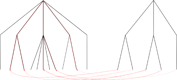
We construct a game with objective . See Figure 1.
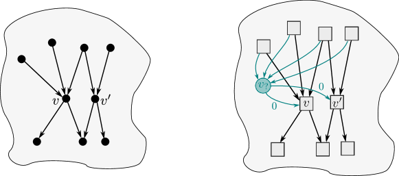
Figure 1. On the left the graph , and on the right the game . The circle depicts the unique vertex which belongs to Eve, while squares belong to Adam. The underlying graph is obtained from with the following modification: the set of vertices is plus a new vertex . All vertices are controlled by Adam except for the new vertex . For every edge leading to either or , we add a new edge going to , where Eve chooses between going to or to with colour . Formally, the sets of vertices and edges are
Eve has a winning strategy from any vertex : each time the play reaches from an edge such that , Eve chooses to continue with , and otherwise with . Any path consistent with this strategy corresponds to a path in , and since satisfies this strategy is winning. We note that this strategy is not positional as it chooses or depending on the incoming edge.
We claim that Eve does not have a positional winning strategy in , which contradicts the positional determinacy of . Indeed, if the positional strategy defined by was winning, since any path in is consistent with in , this would imply that satisfies , contradicting the maximality of . The same argument leads to a contradiction if is a winning strategy.
-
•
Generalised transitivity. Note that left and right composition both generalise transitivity of , that is, (a) and (a) implies (c), by replacing, respectively in (b) or in (a), and in the conclusion (c), the colour 0 with any colour . We prove left composition. Assume that and . We argue by contradiction that . Assuming otherwise, consider a path in . Then obtained from by replacing all occurrences of by is a path in so it must satisfy and hence as well. This contradicts the maximality of . The proof of right composition follows the same lines.
Now to obtain a total order it suffices to refine arbitrarily over its equivalence classes, which preserves left and right compositions. Indeed, two vertices are equivalent for (before refining), that is, are interconnected with -edges, if and only if they have exactly the same -successors and -predecessors for all colours .
4.3. Ubiquity of linear graphs
We now relate linear graphs to the models of Section 3.
Lemma 14.
Let be a linear graph such that . Then
-
•
is an -separating automaton,
-
•
is an -GFSG automaton, and
-
•
is an -universal graph.
Proof 4.4.
By Lemma 12, , so the first item is clear. The second item follows by using the strategy induced by the determinised automaton, that is, .
We now focus on the third item. Let be a graph satisfying and of size at most , and let .
Let be a path ending in in . Then is a prefix of a word in , so is well defined. We now let be defined by
Note that there is always a path ending in since itself is such a path.
We now prove that defines a graph homomorphism. Let , and let be a path in ending in such that . Then is a path in ending in with colour , so we have , and by left composition . This shows that is a homomorphism from to , so is indeed -universal.
We now obtain Theorem 9 as a direct consequence.
5. Solving the product game by value iteration
Section 4 shows that without increasing its size, can be chosen to be a linear graph. In this section, we are interested in the complexity of solving the safety game under this assumption. Fix a game over the graph and a linear graph .
We first give a simplification of in Subsection 5.1 which reduces the size of the arena to vertices and edges. Applying Theorem 2 yields an algorithm with runtime . To further improve the space complexity, we first recall the (well known) linear time algorithm for solving safety games in Subsection 5.2, and then provide in Subsection 5.3 a space efficient implementation of this algorithm over . This reduces the space requirement to . Beyond space efficiency, this section provides an interesting structural insight: solving when is linear precisely amounts to running a value iteration algorithm.
Theorem 15 (Complexity of solving the product game with a linear graph).
Let , an objective, a game of size with prefix independent positional objective , and a linear -universal graph. Then the winning region in can be computed 444In the RAM model with word size . in time and space .
5.1. Simplifying the product game if is linear
We defined the product game for the general case of a non-deterministic automaton . If is linear, the product game can be simplified: from where , Eve should always pick as large a successor in as possible (if there is any successor). More precisely, we let and consider the safety game with vertices and edges given by
In words, from , the player whom belongs to chooses an edge , and the game progresses to if has an outgoing edge with colour in , and to otherwise, which is losing for Eve.
It is clear that Eve wins from in (as defined in Subsection 3.1) if she wins from in , simply by always choosing as a successor from where . The converse is not much harder: just as in the proof of Lemma 12, by an easy induction, picking the largest successor ensures to always remain larger on the second component, which allows for more possibilities (and in particular, avoids sinks) thanks to left composition.
Remark 16.
This also proves that if is in the winning region of and , then is also winning. In particular, is winning in if and only if there exists such that is winning in if and only if is winning in .
From here on, since we solve for linear , we shall use the new (simpler) definition instead of .
5.2. Solving safety games in linear time
We recall the standard linear time algorithm for safety games. Let be a safety game, and consider the operator over subsets of given by
that is, is the set of vertices from which Eve can ensure to remain in for one step. Note that always includes sinks controlled by Adam and excludes sinks controlled by Eve, and it is monotone: if , then .
It is well known that the winning region in is the greatest fixpoint of . This can be computed via Kleene iteration by setting and , which stabilizes in at most steps. Since computing requires operations, a naive implementation yields runtime .
To obtain linear runtime , let us define , the set of vertices which are removed upon applying for the -th time (see Figure 2). Then is the set of sinks controlled by Eve, and moreover we show that for , can be computed efficiently from , provided one maintains a data structure Count, which stores, for each , the number of edges from to . This is based on the observation that a vertex in belongs to if and only if it has an edge towards , and a vertex in belongs to if and only if it has no outgoing edge towards , and moreover it has an edge towards (otherwise, it would not belong to ).
Hence to compute and update Count, it suffices to iterate over all edges such that and : if then , and if , then is decremented, and is added to if 0 is reached, that is, has no edge going to . We give a pseudo-code in Appendix C for completeness. The overall linear complexity of the algorithm simply follows from the fact that each edge is considered at most once.
5.3. Instantiating to : a space efficient implementation
We now instantiate the previous algorithm for safety games to as defined in 5.1.
For a vertex and a set of vertices of , we let . As we have discussed (see Remark 16), the winning region is such that is upward-closed for all . We will see that when instantiating the previous algorithm to , that is, letting and , it always holds that is upward-closed for all , and hence it is specified by its minimal element. Given such that is upward-closed for all , we let be defined by , with value if . We now characterize the effect of over sets represented in this manner. Recall that .
Lemma 17.
Let be such that is upward-closed for all , and let . Then is upward-closed for all , and is given by
Proof 5.1.
Note that for and we have
where the first equivalence holds by right composition while the second holds by left composition.
Let . Then
Hence, is upward-closed, and given by
For replacing ’s by ’s in the previous chain of equivalences yields
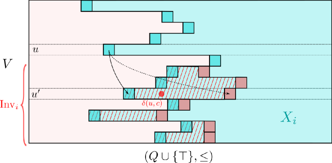
Let and . By a straightforward induction, for all and all , is upward-closed, and we let . By the above lemma, for each , can be computed from the value of at each successor of . Note that by monotonicity of , for each we have . Following the usual terminology for value iteration algorithms, we say that a vertex is invalid at step if , or equivalently, . We let denote the set of vertices which are invalid at step . To compute from , it suffices to update the value of for each . See Figure 3.
Following the previous generic linear time algorithm for solving safety games, we store for each Eve vertex the number of edges from to , which allows to efficiently compute the set of vertices which are invalid at step from those which are invalid at step . We again give a full pseudo-code in Appendix Pseudo-code for generic value iteration algorithm.
Let us conclude with analysing the complexity of the generic value iteration algorithm in the RAM model with word size , in which computing and , checking whether and evaluating require constant time, while storing requires space linear in .
Note that at step , each vertex sees a strict increase in . Hence, there is at most values of such that . Moreover, computing the th update requires, for each , constant-time operations for computing , and constant-time operations for updating Count (at and its predecessors) and computing .
Summing over all vertices, we obtain the wanted time complexity.
Remark 18.
The value iteration algorithm we present here instantiates a linear time implementation of the (global) fixpoint computation to the safety game . There exists a variation of this algorithm which also achieves linear time for solving generic safety games, and works locally: keep a queue of vertices which should be removed from , and a data structure Count storing the number of outgoing edges from to and iteratively pick a vertex from , remove it from , and update Count (potentially adding them to ) on each predecessor of .
It is not hard to instead adapt the local variant of the algorithm to the safety game , which yields another slightly different generic value iteration procedure (with same complexity). The local variant is more in line with known value iteration algorithms for parity games [Jur00, JL17, FJS+17] as well as mean-payoff games [BCD+11, DKZ19]. We chose to present the global variant for its structural simplicity, and direct ties with the fixpoint iteration. For details about the local variant of the generic algorithm, we refer to [FGO20].
This concludes the first part of the paper developing the theory of universal graphs. In the second part, we will consider four (classes of) objectives and construct algorithms from universal graphs.
6. Parity games
The first objective we consider is parity. We refer to Subsection 6.4 for a discussion on existing results.
The set of colours is , where is even and we study the objective given by
In the context of parity games, letters (or colours) are usually called priorities.
We give a convenient characterization of graphs which satisfy the even parity objective. We say that a cycle is even if its maximal priority is even, and odd otherwise.
Lemma 19.
(Graphs satisfying ) Let be a -graph. Then satisfies if and only if all cycles in are even.
Proof 6.1.
Assume that satisfies . Let be a cycle in . Repeating induces an infinite path in with . Then is even, and is even.
Conversely, assume has only even cycles, and pick an infinite path in . Then there is a vertex visited infinitely often by , and then may be decomposed into an infinite sequence of cycles which all start and end in . Then , which is even since for all , is even.
The following well known theorem states that the parity objective satisfies our assumptions.
[[EJ91, McN93, Mos91]] Parity objectives are positionally determined, prefix independent, and have 0 as a neutral letter.
6.1. A universal graph of exponential size
Let us fix a non-negative integer . We give a first construction of a -universal graph . Its set of vertices is given by
that is, tuples of non-negative integers smaller than . Such tuples represent occurrences of odd priorities and for convenience we index with them using odd integers, and in a decreasing fashion, that is, is denoted .
Following [Jur00], we define an increasing sequence of total preorders
over , which are obtained by restricting to the first few values, and comparing lexicographically:
We use to denote the equivalence relation induced by , that is and . We write if . Note that is the full relation: for all we have . At the other end of the scope, is antisymmetric, or in other words its equivalence classes are trivial and coincides with the equality.
The set of edges of is given by
Note that this condition is vacuous for , every pair of vertices is connected (in both directions) by a -edge.
Lemma 20.
The graph is -universal.
Proof 6.2.
We first show that satisfies . Let be an infinite path in , and assume for contradiction that is odd: for all large enough we have , and for infinitely many , . Then for all large enough we have and this inequality is strict for infinitely many ’s, a contradiction.
We now show that embeds all graphs of size which satisfy . Let be such a graph. Let , let be a path from in , and let be an odd priority. Consider the number of occurrences of in before a priority greater than is seen. We claim that , by a pumping argument. Assume for contradiction that , and let denote the first occurrences of in . We have , and for all , . Then the vertices in this order, all have a path with maximal priority to the next one. Since has vertices, there must be a repetition in this sequence, which induces an odd cycle. Given a path , we let .
We now define by , where the max is taken lexicographically over all paths starting in . We claim that defines a graph homomorphism. Let be an edge in and let be a path from in with maximal . Then is a path from in , satisfying if is odd, and for all odd , . If is odd this implies , and if is even we have . In both cases, this yields since .
The set of vertices of can be seen as the set of leaves of the (ordered) complete tree of height and of degree . In this point of view, the equivalence relations groups together leaves which belong to the same subtree at level (where by convention, the leaves are at level 0), hence the equivalence classes correspond to node of level , which are naturally ordered left-to-right by . In other words, a sequence of preorders over some set naturally induces a tree structure of height with leaves .
It is not hard to see that is saturated for the parity objective: the addition of any edge induces an odd cycle. We will actually prove that every saturated graph is given by such a sequence of preorders, which induces the structure of a tree. This will allow us to reformulate the universality condition over parity graphs as a universality condition over trees.
6.2. Trees, tree-like graphs, and saturated parity graphs
Towards describing the structure of saturated graphs for the parity objective, we now define (ordered, levelled) trees.
A tree of height is a finite subset of .
As previously, we think of elements of a tree as representing occurrences of odd priorities. In this regard it is convenient to use odd numbers as indices, and we shall write , where .
A tree of height naturally defines an increasing sequence of total preorders
given by
Again, we use the standard notations relative to total preorders, denotes the equivalence relation associated with , whose equivalence classes are stricly ordered by .
Note that is the full relation, it has one equivalence class. The order is antisymmetric; it is a total order, which coincides with , and coincides with the equality over . Note that there is a unique tree of height which we call the empty tree, and that trees of height are sets of integers.
A tree of height induces a -graph with vertices defined as follows:
-
•
for even , if and only if , and
-
•
for odd , if and only if .
We say that graphs of the form , where is a tree, are tree-like.
Lemma 21.
Let be an even number and a tree of height , then the graph satisfies , and moreover, it is saturated.
Proof 6.3.
We first show that satisfies , which is a direct adaptation of the first part of the proof of Lemma 20. We spell it out for completeness. Let be an infinite path in , and assume for contradiction that is odd: for all large enough we have , and for infinitely many , . Then for all large enough we have and this inequality is strict for infinitely many ’s, a contradiction.
We now show that adding any edge to yields a graph not satisfying . Let be an edge that does not appear in . If is even, then , so the edge belongs to , hence contains an odd cycle. If is odd, then , which implies that the edge belongs to , and again contains an odd cycle.
Now the second part of the proof of Lemma 20 can be re-interpreted as follows.
Lemma 22.
Let be a graph satisfying , where is even. There exists a tree of height and size such that embeds in .
Proof 6.4.
We precisely mimic the proof of Lemma 20. Given a path in and an odd priority , we again define to be the number of occurrences of in before a priority greater than is seen, and we let . It is clear, since satisfies , that all ’s are finite. For , we define to be the lexicographic maximum of ’s over paths starting in , and put .
We prove that defines a homomorphism from to . Let be an edge in and let be a path from in with maximal . Then is a path from in , satisfying if is odd, and for all odd , . If is odd this implies , and if is even we have . In both cases, this yields since .
Actually, it can be shown that, modulo contracting equivalence classes of -edges which have the same ingoing and outgoing edges, saturated graphs are exactly tree-like graphs. This is non-essential for what follows, but we prove it as an interesting side remark.
Lemma 23.
Let be a saturated graph with respect to , where is even, and such that for all , if both and are edges in then . Then there exists a tree of height such that up to renaming the vertices.
Proof 6.5.
By Lemma 22, there exist of height and size and a homomorphism from to . It suffices to prove that is injective. Indeed, this ensures that the sets of vertices of and are in bijection; moreover an edge belongs to whenever belong to since is a homomorphism, and the converse is true by saturation.
Let be such that . We show that and belong to , which implies that . Assume and do not both belong to . Since is saturated, there exists an infinite path in with odd. But by definition of , its vertices, and in particular , have -self-loops, which implies that are edges in . Hence, is a path in with odd limsup, a contradiction.
Interpreting saturated graphs as trees allows us to rephrase the universal property for graphs as a simpler one for trees.
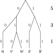
We say that a map where and are trees of height is a tree-homomorphism if it preserves all orderings, that is, for all , and for all odd ,
An example is depicted in Figure 5.
Lemma 24.
Let and be two trees of height , and let . Then is a tree-homomorphism if and only if it is a graph homomorphism from to .
Proof 6.6.
Recall that is the negation of . Hence we have that
the wanted result.
Thanks to Lemma 22 and 24, we may now shift our attention only to trees and their homomorphisms. We say that a tree is -universal if it has height and embeds all trees of height and size .
Lemma 25.
The smallest -universal trees and the smallest -universal graphs have the same size.
Proof 6.7.
Let be a -universal graph. By Lemma 22, there is a tree of height not larger than and such that embeds into . Let be a tree of height and size . By universality of , there is a homomorphism from to , which by composition induces a homomorphism from to . We conclude by Lemma 24 that embeds , and hence is -universal.
Conversely, let be -universal, and let be a graph satisfying . By Lemma 22 there is a tree of height such that maps into . Now maps into by universality, by Lemma 24, this translates into a map from to , and finally by composition on the left, maps into . We conclude that is -universal, and it has the same size as .
6.3. Upper and lower bounds on universal trees
We now study the size of the smallest -universal trees. In this subsection, we simply index elements of trees of height with integers from to for clarity.
Theorem 26.
Let .
-
•
There exists a -universal tree of size at most
-
•
All -universal trees have size at least
Let us start with the upper bound.
Proposition 27.
There exists a -universal tree with size , where satisfies the following recursion
We refer to Appendix A for an analysis of this recurrence, leading to the upper bound stated in Theorem 26. We further analyse this function when presenting the induced algorithm in Subsection 6.4.
Proof 6.8.
We construct a -universal tree by induction over , lexicographically. Trees of height and size are (downward-closed) subsets of , hence is -universal. There is a unique tree of size and height , namely, , and it is -universal. Now, let and be and assume constructed -universal trees of size for each . Let
-
•
be a -universal tree,
-
•
be a -universal tree, and
-
•
be a -universal tree.
Intuitively, we construct by merging the roots of and of and inserting in between a child of the root to which is attached.
Formally, we let be the number of children of , and put
We now argue that is -universal. Consider a tree of height and size . We let be the number of children of . For each , let be the number of leaves in the -th child of , that is, . Since , there is such that and , which implies .
Consider the three trees , and .
The trees and have height and respective sizes and , hence they map respectively, via and into and . Likewise, the tree has height and size at most , hence it has a homomorphism into . These are combined into a map from to by
We now prove that is indeed a tree-homomorphism from to . Let and let . If and are either both , both , or both , then they both correspond to vertices of or of or of , and we conclude that by invoking the fact that either or is a tree-homomorphism. Otherwise, without loss of generality , and we even have with one of these inequalities being strict, hence , whatever the value of . By definition of we have with the same inequality being strict, which likewise implies that , the wanted result. Hence is universal, which concludes the proof.
We now prove a lower bound on the size of universal trees.
Proposition 28.
Any -universal tree has at size at least , where satisfies the following recursion
We refer to Appendix B for an analysis of this recurrence, leading to the lower bound stated in Theorem 26.
The upper and lower bounds do not match perfectly. However,
i.e. they are polynomially related.
Proof 6.9.
The bounds are clear for or . We let assumed the result known for , and let be a -universal tree, and we let . We construct a tree of height by restricting to subtrees of height 1 which have children, that is
and argue that is -universal.
Indeed, let be a tree of height with leaves. To each leaf of we append children, that is, we consider
which has size and height . Since is -universal, there is a tree-homomorphism from to . Now, for each , the elements of are different and -equivalent in , hence so must be their image in . As a consequence, defined by satisfies , or in other words, , and preserves all orders just because does. Hence, embeds in , and we conclude that is -universal.
In particular, the induction hypothesis tells us that has size at least . Summing over values of , we count each -equivalent class of as many times as its size, which concludes with the wanted bound.
6.4. The complexity of solving parity games using universal graphs
Let us start with reviewing the recent results on parity games and their relationships with separating automata, GFSG automata, and universal trees.
The first quasipolynomial time algorithm comes in three flavours: the original version [CJK+17], as a value iteration algorithm [FJS+17], and as a separating automaton [BC18]. The second quasipolynomial time algorithm called succinct progress measure lifting algorithm [JL17] is a value iteration algorithm; it was presented using the formalism of universal trees in [Fij18], and then as a separating automaton in [CDF+18].
Hence deterministic models (separating automata) are expressive enough to capture the first two algorithms; the situation changes with the register games algorithm [Leh18]. Indeed it was observed in [CDF+18] that the algorithm induces a ‘non-deterministic separating automaton’, meaning an automaton satisfying ; this was enough to subject this third algorithm to the lower bound on the size of separating automata since the result of [CDF+18] applies to non-deterministic automata (in the same way as Theorem 9 does). However this is not enough to prove the correctness of the construction: under this assumption the two games and may not be equivalent. The follow-up paper [Par20] investigated this issue and offered a sufficient condition for a non-deterministic separating automaton to ensure the equivalence between and . This condition is almost the same as the good-for-small-games condition we introduced independently in [CF19], the only differences are that in the framework of [Par20] the automata read edges (meaning triples ) while here the automata only read priorities, and the good-for-small-games strategy depends on the graph. The journal version of the register games algorithm suggested the name ‘good-for-small-games’ [LB20].
We further discuss in the conclusions section (Section 10) the recent extensions of the register games algorithm.
The main conclusion of our studies on universal graphs and trees is the following algorithm, combining Theorem 26 and Theorem 15.
Corollary 29.
Let . There exists an algorithm555In the RAM model with word size . solving parity games with vertices, edges, and priorities in in time
A generous upper bound on the expression above is . A refined calculation reveals that the expression is polynomial in and if . We refer to [JL17] for the tightest existing analysis of the binomial coefficient.
The choice of word size is inherited from the generic value iteration algorithm using word size , because . For this word size it is easy to verify that the two following operations on universal trees take constant time: computing and comparing . Choosing the word size implies that a leaf of the universal tree cannot anymore be represented in a single machine word: the ‘succinct encoding’ proposed in [JL17] performs the two operations above in a very low complexity (polylogarithmic in time) in this setting.
The complexity of (variants of) this algorithm has been investigated by Chatterjee, Dvorák, Henzinger, and Svozil in the set-based symbolic model [CDHS18], which is a different computational model; the differences are only in polynomial factors.
The second outcome of our analysis is a lower bound argument.
Corollary 30.
All algorithms based on separating automata, GFSG automata, or universal graphs, have at least quasipolynomial complexity.
This extends the main result of [CDF+18] which stated this result using non-deterministic separating automata and universal trees. The statement is kept informal since its value is not in its exact formalisation but in the perspectives it offers: all existing quasipolynomial time algorithms for parity games have been tightly related to the notion of universal trees. Corollary 30 states that to improve further the complexity of solving parity games one needs to go beyond the notion of universal trees.
7. Mean payoff
The second objective we consider is mean payoff. We refer to Subsection 7.3 for a discussion on existing results.
The set of colours is a finite set with , and in this context they are called weights.
In this section we consider graphs over the set of colours .
Let us state a characterisation of graphs satisfying in terms of cycles. We say that a cycle is non-negative if the total sum of weights appearing on the cycle is non-negative, and negative otherwise.
Lemma 31.
Let be a graph. Then satisfies if and only if all cycles in are non-negative.
Proof 7.1.
Assume that satisfies . A cycle induces an infinite path, and since the path satisfies the cycle is non-negative. Conversely, if does not satisfy , a simple pumping argument implies that it contains a negative cycle.
The following theorem states that the mean payoff objectives satisfy our assumptions.
[[EM79, GKK88]] Mean payoff objectives are positionally determined, prefix independent, and have as neutral letter.
The goals of this section are to:
-
•
describe the structure of saturated graphs and in particular its relation with integer subsets,
-
•
construct universal graphs for different mean payoff conditions,
-
•
derive from these constructions efficient algorithms for solving mean payoff games,
-
•
offer (asymptotically) matching lower bounds on the size of universal graphs, proving the optimality of the algorithms in this family of algorithms.
7.1. Subsets of the integers and saturated graphs
Towards understanding their structure we study the properties of saturated graphs and show that they are better presented using subsets of the integers. A subset of integers defines a graph which we call an integer graph: the set of vertices is and the set of edges is
Note that the definition depends on . Integer graphs contain no negative cycles and are invariant under translations: and for induce the same integer graph (up to renaming vertices).
The key yet simple observation at this point is that given a graph with no negative cycles
we can define a distance between vertices:
the distance from a vertex to another vertex
is the smallest sum of the weights along a path from to (when such a path exists).
Note that saturated graphs with respect to are linear by Theorem 13.
In particular, they have a maximal element.
Lemma 32.
Let be a saturated graph and its maximal element. Let
then maps into .
Proof 7.2.
We show that defined by is a homomorphism from to . Since is maximal, by right-composition with the -self-loop on , for every vertex there is an edge . This implies that is well defined, and non-negative. Let , then since a path from to induces a path from to by adding at the end. In other words, , so is indeed a homomorphism.
The direct consequences of Lemma 32 is that we can restrict our attention to integer graphs.
Corollary 33.
Let and .
-
•
The smallest -universal graph and the smallest -universal integer graph have the same size.
-
•
An integer graph is -universal if and only if every integer graph of size at most maps into .
Proof 7.3.
For the first item, if is -universal, without loss of generality it is saturated, then maps into the integer graph constructed in Lemma 32, so the latter is also -universal. For the second item, the direct implication is clear so we focus on the converse. Let us assume that every integer graph of size at most maps into and prove that is -universal. Let be a graph of size at most satisfying , thanks to Lemma 32 it maps into an integer graph of the same size, which then maps into , so by composition maps into .
7.2. Upper and lower bounds for universal graphs
We now state in the following theorem upper and lower bounds on the size of universal graphs. We present two sets of results based on : the first is parametrised by the largest weight in absolute value, and the second by the number of different weights.
Theorem 34 (Universal graphs parameterized by largest weight).
Let , and .
-
•
There exist -universal graphs of size and of size .
-
•
All -universal graphs have size at least .
Theorem 35 (Universal graphs parameterised by the number of weights).
-
•
For all and of cardinality , there exists an -universal graph of size .
-
•
For all and for all large enough, there exists of cardinality such that all -universal graphs have size .
Let us start with simple upper bounds.
Lemma 36.
Let .
-
•
The integer graph is -universal.
-
•
For every of cardinality , there exists an -universal graph of size .
Proof 7.4.
We show both results at the same time.
Let be a graph of size at most satisfying , and a saturation of , thanks to Lemma 32 maps into , implying that as well.
In the case where we have so maps into . This proves that the integer graph is -universal.
In the case where we consider the set of all sums of weights of , which has cardinality at most . Then so maps into . This proves that is -universal and it has size .
We state here a simple result that we will use several times later on about homomorphisms into integer graphs.
Fact 37.
Let be a graph and a homomorphism into an integer graph. Let us consider a cycle in of total weight . Then for , we have , where by convention .
Proof 7.5.
By definition of the homomorphism using the edges for
Assume towards contradiction that one of these inequalities is strict. Summing all of them yields on both sides (because the cycle has total weight ), so this would imply , a contradiction. Hence all inequalities are indeed equalities.
We further analyse universal graphs when . We already explained in Lemma 36 how to construct an -universal graphs of size . We improve on this upper bound when is exponential in .
Proposition 38.
There exists an -universal graph of size
As discussed above, the size of this new universal graph is not always smaller than the first universal graph of size , but it is asymptotically smaller when . We now give some intuition for the construction. The first part of the proof of Lemma 36 shows that it suffices to embed integer graphs of the form , when for some graph . In the above proof, this was done by finding a large enough set of integers that includes any such : in the first case and in the second case . To conclude we used the fact that if then there exists a homomorphism from to .
A weaker condition is the existence of such that : this still implies the existence of a homomorphism from to . This will allow us to remove some values from while remaining universal. As a drawback we need to double the range to , which explains why this new construction is not always smaller than the first one.
Proof 7.6.
Let . We write integers in basis , hence using digits written , that is,
Note that since the th digit is either or . We let be the set of integers in which have at least one zero digit among the first digits in this decomposition. We argue that is -universal.
Let be a graph of size at most satisfying , to show that maps into we use Lemma 32 and show that for , the graph maps into . To this end we show that there exists such that .
Let , where , and for all , we have .
We choose of the form for , i.e. the th digit is , or equivalently . Let us write , for . We need to choose such that for every we have . Note that for all it holds that , so whatever the choice of , we have .
We show how to choose in order to ensure that , that is, each have at least one digit among the first ones which is zero. More precisely, we show by induction on that there exist such that for any choice of and for all , the -th digit of is . For , we let , which yields , independently of the values of .
Let be such that for any choice of , for any , we have . Let be the (unique) value such that . Let . By induction hypothesis, for any , we have . Now
since both terms are zero. This concludes the inductive construction of , and the proof of universality of . Since excludes from exactly integers (those that do not use the digit in their first digits), the size of is
We now prove the lower bound of Theorem 34.
Proposition 39.
Any -universal graph has size at least .
Proof 7.7.
Thanks to Lemma 32, we let be an -universal integer-graph given by . We construct an injective function . For , we consider , with and for .
By universality, maps into , and we let be such a homomorphism. Define to be the -tuple of integer in given by
To see that is injective, we apply Fact 37 to each cycle of length 2 in of the form
for . This yields
and is injective. We conclude that , so .
Proposition 40.
Let be an -universal graph. Then
Proof 7.8.
Let be an -universal graph.
We consider a class of graphs which are cycles of length , and later use a subset of those for the lower bound. Let . The vertices are . There is an edge for and an edge . To make the total weight in the cycle equal to , we assume that each appears exactly many times in .
The cycles we use for the lower bound are described in the following way. We let be the set of sequences of integers in such that , where we use the notation for an element . A tuple of sequences in induces a graph . Let , the induced graph is partitioned into parts. In the th part the weight is used exactly many times. See Figure 9.
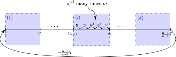
The vertex in marking the end of the first box is , and more generally the vertex marking the end of the th box is
Note that is the th digit of the number in base , since it belongs to , and so it is . Hence, fully determines the sequences . We also let .
Let be a homomorphism. We define a function by , which we prove to be injective. The constraint on the sums of sequences on ensures that indeed the graph is a cycle of total weight , and then thanks to Lemma 37 applied to the cycle , we have
and as explained above the numbers fully determine the sequences .
Injectivity of implies that . The size of is
which implies (for constant) .
7.3. The complexity of solving mean payoff games using universal graphs
There is a very large literature on mean payoff games, a model independently introduced by Ehrenfeucht and Mycielski [EM79] and by Gurvich, Karzanov, and Khachiyan [GKK88] and studied in different research communities including program verification and optimisation. The seminal paper of Zwick and Paterson [ZP96] relates mean payoff games to discounted payoff games and simple stochastic games, and most relevant to our work, constructs an algorithm for solving mean payoff games with complexity , where is the number of vertices, the number of edges, and the largest weight in absolute value. If the weights are given in unary is polynomial in the representation, so we say that the algorithm is pseudo-polynomial. The question whether there exists a polynomial time algorithm for mean payoff games with the usual representation of weights, meaning in binary, is open. The currently fastest algorithm for mean payoff games is randomised and achieves subexponential complexity . It is based on randomised pivoting rules for the simplex algorithm devised by Kalai [Kal92, Kal97] and Matoušek, Sharir and Welzl [MSW96].
We are in this work interested in deterministic algorithms for solving mean payoff games. Up until recently there were two fastest deterministic algorithms: the value iteration algorithm of Brim, Chaloupka, Doyen, Gentilini, and Raskin [BCD+11], which has complexity , and the algorithm of Lifshits and Pavlov [LP07] with complexity . They are incomparable: the former is better when and otherwise the latter prevails. Recently Dorfman, Kaplan, and Zwick [DKZ19] presented an improved version of the value iteration algorithm with a complexity , an improvement over the previous two algorithms when .
Solving a mean payoff game is very related to constructing an optimal strategy, meaning one achieving the highest possible value. The state of the art for this problem is due to Comin and Rizzi [CR17] who designed a pseudo-polynomial time algorithm.
Let us now construct algorithms from universal graphs combining Theorem 34 and Theorem 35 with Theorem 15.
Corollary 41.
Let . The following statements use the RAM model with word size .
-
•
There exists an algorithm for solving mean payoff games with weights in of time complexity and space complexity .
-
•
There exists an algorithm for solving mean payoff games with weights in of time complexity and with space complexity .
-
•
There exists an algorithm for solving mean payoff games with weights of time complexity and space complexity .
The first algorithm is exactly the algorithm constructed by Brim, Chaloupka, Doyen, Gentilini, and Raskin [BCD+11]: identical data structures and complexity analysis. The two tasks for manipulating universal graphs, namely computing and checking whether are indeed unitary operations as they manipulate numbers of order .
Let us now discuss the significance of the difference between to , meaning the first and second algorithms. Since is polynomial in the size of the input, one may say that is “small”, while is exponential in the size of the input when weights are given in binary, hence “large”. For we have so is essentially linear in . However when for then , so the second algorithm is indeed asymptotically faster. To appreciate the relevance of this condition, let us recall an old result of Frank and Tardos [FT87] which implies that one can in polynomial time transform a mean payoff game into an equivalent one where . Our new algorithm improves over the previous one for the range . We note however that the recent algorithm [DKZ19] (building over [BCD+11] and [GKK88]) is always faster than the second algorithm.
As for the case of parity games, the lower bounds presented in Theorem 34 and Theorem 35 show that to obtain faster algorithms we need to go beyond algorithms based on universal graphs. In particular there are no quasipolynomial universal graphs for mean payoff objectives, and the question whether the quasipolynomial time algorithms for parity games can be extended to mean payoff games remains open.
8. Disjunction of a parity and a mean payoff objective
The third objective is the disjunction of parity and mean payoff objectives. We refer to Subsection 8.2 for a discussion on existing results.
The set of colours is for some with . For we write for the projection on the first component and for the projection on the second component. We define as
The following theorem states that disjunctions of parity and mean payoff objectives satisfy our assumptions.
[[CHJ05]] Disjunctions of parity and mean payoff objectives are positionally determined, prefix independent, and have as neutral letter.
Our approach for constructing universal graphs for disjunctions of parity and mean payoff objectives differs from the previous two cases. Here we will rely on the existing constructions of universal graphs for parity and for mean payoff objectives, and show general principles for combining universal graphs for disjunctions of objectives.
It is here technically more convenient to reason with separating automata, taking advantage of determinism. Thanks to Theorem 9 this is equivalent in terms of complexity of the obtained algorithms.
8.1. Separating automata for disjunctions of parity and mean payoff objectives
Theorem 42.
Let , an -separating automaton, and an -separating automaton. Then there exists an -separating automaton of size .
Proof 8.1.
Let us write and . We define a deterministic automaton : the set of states is , the initial state is , and the transition function is defined as follows: is equal to
Intuitively: simulates the automaton , storing the maximal priority seen since the last reset (or from the beginning). If the automaton rejects, the automaton resets, which means two things: it simulates one transition of the automaton using the stored priority, and resets the state of to its initial state. The automaton rejects only if rejects during a reset.
We now prove that is an -separating automaton.
-
•
. Let be an infinite path accepted by , we distinguish two cases by looking at the run of .
-
–
If the run is reset finitely many times, let us write where is finite and rejected by , and is infinite and is accepted by . Since satisfies , this implies that satisfies , so by prefix independence, satisfies hence satisfies .
-
–
If the run is reset infinitely many times, we may find an infinite decomposition where for each , the path is rejected by , and its proper prefixes are not. Let be the maximum priority appearing in , the run of over induces a run of over . Since satisfies , this implies that satisfies . By definition of the ’s, this implies that satisfies so a fortiori satisfies .
-
–
-
•
. Let be a graph satisfying of size at most , we need to show that all infinite paths of are accepted by .
We construct a graph over the set of colours and a graph over the set of colours . Both use the same set of vertices as . We prove that the graph satisfies , which is used to prove that satisfies .
-
–
The graph . There is an edge if there exists such that , and either is odd or is even and is not contained in any negative cycle with maximum priority .
We claim that satisfies . Assume towards contradiction that contains a negative cycle . It induces a negative cycle in , by definition of necessarily the maximum priority in is odd. Hence is a negative odd cycle in , a contradiction.
-
–
The graph . There is an edge if there exists a path in from to with maximum priority and (whose projection on the mean payoff component is) rejected by .
We claim that satisfies . Assume towards contradiction that contains an odd cycle . For each edge in this cycle there is a corresponding path rejected by with the same maximum priority. Putting these paths together yields an odd cycle , of maximal priority , in whose projection on the mean payoff component is rejected by . Since and as we have shown, satisfies , the projection of on the mean payoff component is not in , so there exists an edge in such that is not in . This implies that is even, so in particular , and is contained in a negative cycle in with maximum priority . Combining the odd cycle followed by sufficiently many iterations of the negative cycle yields a path in , with negative weight, and maximal priority which is odd, a contradiction.
Let an infinite path in , we show that is accepted by . Let us consider first only the mean payoff component: we run repeatedly over , and distinguish two cases.
-
–
If there are finitely many resets, let us write where are paths rejected by with proper prefixes accepted by and is accepted by . To show that is accepted by we need to show that the automaton accepts the word where is the maximum priority appearing in for . Indeed, is a path in , which is a graph of satisfying , so accepts .
-
–
If there are infinitely many resets, let us write where for each , the path is rejected by and its proper prefixes are not. To show that is accepted by we need to show that the automaton accepts the word , which holds for the same reason as the other case: is a path in .
-
–
8.2. The complexity of solving disjunctions of parity and mean payoff games using separating automata
The class of games with a disjunction of a parity and a mean payoff objective has been introduced in [CHJ05], with a twist: this paper studies the case of a conjunction instead of a disjunction, which is more natural in many applications. This is equivalent here since both parity and mean payoff objectives are dual, in other words if the objective of Eve is a disjunction of a parity and a mean payoff objective, then the objective of Adam is a conjunction of a parity and a mean payoff objective. Hence all existing results apply here with suitable changes. The reason why we consider the objective of the opponent is that it is positionally determined, which is the key assumption for using the universal graph technology.
The state of the art for solving disjunctions of parity and mean payoff games is due to [DJL18], which presents a pseudo-quasi-polynomial algorithm. We refer to [DJL18] for references on previous studies for this class of games. As they explain, these games are logarithmic space equivalent to the same games replacing mean payoff by energy, and polynomial time equivalent to games with weights [SWZ19], extending games with costs [FZ14].
Theorem 43.
Let . There exists an algorithm 666In the RAM model with word size . for solving disjunctions of parity and mean payoff games with vertices, edges, weights in and priorities in of time complexity
and space complexity .
Our algorithm is similar to the one constructed in [DJL18]: they are both value iteration algorithms (called progress measure lifting algorithm in [DJL18]), combining the two value iteration algorithms for parity and mean payoff games. However, the set of values are not the same (our algorithm stores an additional priority) and the proofs are very different. Besides being much shorter777The only generic result we use from universal graphs here is the equivalence between and when is a separating automaton., one advantage of our proof is that it works with abstract universal graphs for both parity and mean payoff objectives, and shows how to combine them, whereas in [DJL18] the proof is done from scratch, extending both proofs for the parity and mean payoff objectives.
9. Disjunction of mean payoff objectives
The fourth objective we consider is disjunctions of mean payoff objectives. We refer to Subsection 9.3 for a discussion on existing results.
The set of colours is a finite set for some with . For and we write for the projection on the -th component.
The following theorem states that disjunctions of mean payoff objectives satisfy our assumptions.
Theorem 44 (Lemma 9 in [VCD+15]).
Disjunctions of mean payoff objectives are positionally determined, prefix independent, and have as neutral letter.
To obtain a universal graph for disjunctions of mean payoff objectives, we will show how to combine the existing constructions for mean payoff objectives.
9.1. A general reduction of universal graphs for strongly connected graphs
The first idea is very general, it roughly says that if we know how to construct universal graphs for strongly connected graphs, then we can use them to construct universal graphs for general graphs.
We say that a graph is strongly connected if for every pair of vertices there exists a path from one vertex to the other. Let us refine the notion of universal graphs.
[Universal graphs for strongly connected graphs] A graph is -universal for strongly connected graphs if it satisfies and all strongly connected graphs of size at most satisfying map into .
Let us give a first construction, which we refine later. Let and be two graphs, we define their sequential product as follows: the set of vertices is , and the set of edges is
The sequential product is extended inductively: . Intuitively, is the disjoint union of the graphs ’s with all possible forward edges from to for any .
Lemma 45.
Let be a prefix independent objective, , and an -universal graph for strongly connected graphs. Then is an -universal graph.
Proof 9.1.
We first note that any infinite path in eventually remains in one copy of . Since satisfies and by prefix independence of , this implies that the infinite path satisfies , thus so does .
Let be a graph satisfying , we show that maps into . We decompose into strongly connected components: let be the maximal strongly connected components in indexed such that if there exists an edge from to then . Then is the disjoint union of the ’s. Each is a subgraph of , and since satisfies then so does . It follows that each maps into , let be a homomorphism .
Let us define by if . We now argue that is a homomorphism . Let , then either , and then belongs to because is a homomorphism, or goes from to with , and then again is an edge in . Thus is a homomorphism and therefore is -universal.
In the construction above we have used the fact that decomposes into at most strongly connected components of size . We refine this argument: the total size of the strongly connected components is . The issue we are facing in taking advantage of this observation is that the sequence of sizes is not known a priori, it depends on the graph. To address this we use a universal sequence. First, here a sequence means a finite sequence of non-negative integer, for instance . The size of a sequence is the total sum of its elements, so has size . We say that embeds into if there exists an increasing function such that for all , we have . For example embeds into but not in . A sequence is -universal if all sequences of size at most embed into .
Remark 46.
The notion of -universal sequence is equivalent to that of -universal trees: a tree of height is given by a sequence consisting of the number of leaves of each subtree of height . This explains why the constructions that follow may feel familiar after reading Section 6.
Let us define an -universal sequence , inductively on . We set (the empty sequence), , and is the concatenation of with the singleton sequence followed by . Writing for concatenation, the definition reads Let us write the first sequences:
Lemma 47.
The sequence is -universal and has size .
Proof 9.2.
We proceed by induction on . The case is clear, let us assume that . Let be a sequence of size , we show that embeds into . There exists a unique such that has size smaller than or equal to and has size larger than . This implies that has size at most . By induction hypothesis embeds into and embeds into , so embeds into .
The recurrence on size is , it implies that is bounded by .
We now use the universal sequence to improve on Lemma 45
Lemma 48.
Let be a positionally determined prefix independent objective and . For each , let be a -universal graph for strongly connected graphs. Let us write , then is an -universal graph.
Proof 9.3.
We follow the same lines as for Lemma 45, in particular the same argument implies that satisfies .
Let be a graph satisfying , we show that maps into . We decompose into strongly connected components as before. Let us write the sequence of sizes of the components. The sequence has size at most , implying that embeds into : there exists an increasing function such that for all we have . It follows that for each , there exists a homomorphism .
Let us define by if . We now argue that is a homomorphism . Let , then either , and then is an edge in because is a homomorphism, or goes from to with , and then the same holds because is increasing. Thus is a homomorphism and is -universal.
9.2. Universal graphs for disjunctions of mean payoff objectives
We state in the following theorem an upper bound on the construction of universal graphs for disjunctions of mean payoff objectives.
Theorem 50.
Let and of largest weight in absolute value . There exists an -universal graph of size .
As suggested by the previous subsection, we first construct -universal graphs for strongly connected components. The following result shows a decomposition property.
Lemma 51.
Let be a strongly connected graph and . Assume that satisfies then there exists such that satisfies .
Proof 9.4.
We prove the contrapositive: assume that for all the graph does not satisfy , implying that for each there exists a negative cycle around some vertex . By iterating each cycle an increasing number of times, we construct a path in which does not satisfy .
To make this statement formal, we use the following property: for any , any finite path can be extended to a finite path with weight on the th component. This is achieved simply by first going to using strong connectedness, then iterating through cycle a sufficient number of times.
We then apply this process repeatedly and in a cyclic way over to construct an infinite path such that for each , infinitely many times the -th component is less than . This produces a path which does not satisfy , a contradiction.
Note that the above proof relies on the semantics that we assumed for defining . No similar simple decomposition is known for the semantics, which turns out to be much harder (it is in fact NP-complete even when is fixed [VCD+15]).
Corollary 52.
Let , and be an -universal graph for strongly connected graphs. We construct the disjoint union of copies of , where the -th copy reads the -th component. Then is an -universal graph for strongly connected graphs.
We can now prove Theorem 50.
9.3. The complexity of solving disjunctions of mean payoff games using universal graphs
Let us note here that there are actually two variants of the mean payoff objective: using infimum limit or supremum limit. In many cases the two variants are equivalent: this is the case when considering mean payoff games or disjunctions of parity and mean payoff games. However, this is not true anymore for disjunctions of mean payoff objectives, as explained in [VCD+15]. Our constructions and results apply using the infimum limit, and do not extend to the supremum limit.
The main result related to disjunction of mean payoff games in [VCD+15] (Theorem 6) is that the problem is in and can be solved in time . (Note that since we consider the dual objectives, the infimum limit becomes a supremum limit in [VCD+15].)
Corollary 53.
Let . In the RAM model with word size , there exists an algorithm for solving disjunctions of mean payoff games with weights in with time complexity and space complexity .
Note that for the choice of word size, the two tasks for manipulating universal graphs, namely computing and checking whether are indeed unitary operations as they manipulate numbers of order .
10. Conclusions
In this paper we have introduced the notion of universal graphs for constructing generic value iteration algorithms for games with positionally determined objectives. We have instantiated this to four classes of games, achieving or improving the state of the art for solving these games. There are many other potential applications, for instance Rabin objectives or disjunctions of parity objectives.
We laid the first brick for the theory of universal graphs, and we hope that this new tool will open new perspectives. An exciting research direction is to construct universal graphs for subclasses of graphs. For instance, it is known that solving parity games over graphs of bounded tree width or clique width is polynomial [Obd03, Obd07]. Are there universal graphs of polynomial size for these classes of graphs? A step in this direction was made recently by Daviaud, Jurdziński, and Thejaswini [DJT20]: revisiting the register games algorithm [Leh18, LB20], they introduced a new parameter called the Strahler number and constructed universal trees for bounded Strahler numbers.
Another promising direction is to extend the use of universal graphs from games to automata. The first brick in the wall was thrown by Daviaud, Jurdziński, and Lehtinen [DJL19], who showed that universal trees can be used to improve constructions for alternating automata over infinite words.
References
- [BC18] Mikołaj Bojańczyk and Wojciech Czerwiński. An automata toolbox, February 2018. https://www.mimuw.edu.pl/~bojan/papers/toolbox-reduced-feb6.pdf.
- [BCD+11] Lubos Brim, Jakub Chaloupka, Laurent Doyen, Raffaella Gentilini, and Jean-François Raskin. Faster algorithms for mean-payoff games. Formal Methods in System Design, 38(2):97–118, 2011. doi:10.1007/s10703-010-0105-x.
- [CDF+18] Wojciech Czerwiński, Laure Daviaud, Nathanaël Fijalkow, Marcin Jurdziński, Ranko Lazić, and Paweł Parys. Universal trees grow inside separating automata: Quasi-polynomial lower bounds for parity games. CoRR, abs/1807.10546, 2018. arXiv:1807.10546.
- [CDHS18] Krishnendu Chatterjee, Wolfgang Dvorák, Monika Henzinger, and Alexander Svozil. Quasipolynomial set-based symbolic algorithms for parity games. In LPAR, pages 233–253, 2018.
- [CF16] Thomas Colcombet and Nathanaël Fijalkow. The bridge between regular cost functions and -regular languages. In ICALP, pages 126:1–126:13, 2016. doi:10.4230/LIPIcs.ICALP.2016.126.
- [CF18] Thomas Colcombet and Nathanaël Fijalkow. Parity games and universal graphs. CoRR, abs/1810.05106, 2018. arXiv:1810.05106.
- [CF19] Thomas Colcombet and Nathanaël Fijalkow. Universal graphs and good for games automata: New tools for infinite duration games. In FoSSaCS, pages 1–26, 2019. doi:10.1007/978-3-030-17127-8\_1.
- [CHJ05] Krishnendu Chatterjee, Thomas A. Henzinger, and Marcin Jurdziński. Mean-payoff parity games. In LICS, pages 178–187, 2005. doi:10.1109/LICS.2005.26.
- [CJK+17] Cristian S. Calude, Sanjay Jain, Bakhadyr Khoussainov, Wei Li, and Frank Stephan. Deciding parity games in quasipolynomial time. In STOC, pages 252–263, 2017. doi:10.1145/3055399.3055409.
- [Col09] Thomas Colcombet. The theory of stabilisation monoids and regular cost functions. In ICALP, 2009.
- [CR17] Carlo Comin and Romeo Rizzi. Improved pseudo-polynomial bound for the value problem and optimal strategy synthesis in mean payoff games. Algorithmica, 77(4):995–1021, 2017. doi:10.1007/s00453-016-0123-1.
- [DJL18] Laure Daviaud, Marcin Jurdziński, and Ranko Lazić. A pseudo-quasi-polynomial algorithm for mean-payoff parity games. In LICS, pages 325–334, 2018. doi:10.1145/3209108.3209162.
- [DJL19] Laure Daviaud, Marcin Jurdziński, and Karoliina Lehtinen. Alternating weak automata from universal trees. In Wan J. Fokkink and Rob van Glabbeek, editors, CONCUR, volume 140 of LIPIcs, pages 18:1–18:14. Schloss Dagstuhl - Leibniz-Zentrum für Informatik, 2019. doi:10.4230/LIPIcs.CONCUR.2019.18.
- [DJT20] Laure Daviaud, Marcin Jurdziński, and K. S. Thejaswini. The strahler number of a parity game. In Artur Czumaj, Anuj Dawar, and Emanuela Merelli, editors, ICALP, volume 168 of LIPIcs, pages 123:1–123:19. Schloss Dagstuhl - Leibniz-Zentrum für Informatik, 2020. doi:10.4230/LIPIcs.ICALP.2020.123.
- [DKZ19] Dani Dorfman, Haim Kaplan, and Uri Zwick. A faster deterministic exponential time algorithm for energy games and mean payoff games. In ICALP, pages 114:1–114:14, 2019. doi:10.4230/LIPIcs.ICALP.2019.114.
- [EJ91] E. Allen Emerson and Charanjit S. Jutla. Tree automata, -calculus and determinacy. In FOCS, pages 368–377. IEEE Computer Society, 1991.
- [EM79] Andrzej Ehrenfeucht and Jan Mycielski. Positional strategies for mean payoff games. International Journal of Game Theory, 109(8):109–113, 1979. doi:10.1007/BF01768705.
- [FGO20] Nathanaël Fijalkow, Paweł Gawrychowski, and Pierre Ohlmann. Value iteration using universal graphs and the complexity of mean payoff games. In MFCS, volume 170 of LIPIcs, pages 34:1–34:15. Schloss Dagstuhl - Leibniz-Zentrum für Informatik, 2020. doi:10.4230/LIPIcs.MFCS.2020.34.
- [Fij18] Nathanaël Fijalkow. An optimal value iteration algorithm for parity games. CoRR, abs/1801.09618, 2018. arXiv:1801.09618.
- [FJS+17] John Fearnley, Sanjay Jain, Sven Schewe, Frank Stephan, and Dominik Wojtczak. An ordered approach to solving parity games in quasi polynomial time and quasi linear space. In SPIN, pages 112–121, 2017.
- [FT87] András Frank and Éva Tardos. An application of simultaneous diophantine approximation in combinatorial optimization. Combinatorica, 7(1):49–65, 1987. doi:10.1007/BF02579200.
- [FZ14] Nathanaël Fijalkow and Martin Zimmermann. Parity and streett games with costs. Logical Methods in Computer Science, 10(2), 2014. doi:10.2168/LMCS-10(2:14)2014.
- [GKK88] Vladimir A. Gurvich, Aleksander V. Karzanov, and Leonid G. Khachiyan. Cyclic games and an algorithm to find minimax cycle means in directed graphs. USSR Computational Mathematics and Mathematical Physics, 28:85–91, 1988.
- [HP06] Thomas A. Henzinger and Nir Piterman. Solving games without determinization. In CSL, pages 395–410, 2006.
- [JL17] Marcin Jurdziński and Ranko Lazić. Succinct progress measures for solving parity games. In LICS, pages 1–9, 2017.
- [JM20] Marcin Jurdziński and Rémi Morvan. A universal attractor decomposition algorithm for parity games. CoRR, abs/2001.04333, 2020. arXiv:2001.04333.
- [JMOT20] Marcin Jurdziński, Rémi Morvan, Pierre Ohlmann, and K. S. Thejaswini. A symmetric attractor-decomposition lifting algorithm for parity games. CoRR, abs/2010.08288, 2020. URL: https://arxiv.org/abs/2010.08288, arXiv:2010.08288.
- [Jur00] Marcin Jurdziński. Small progress measures for solving parity games. In STACS, pages 290–301, 2000. doi:10.1007/3-540-46541-3\_24.
- [Kal92] Gil Kalai. A subexponential randomized simplex algorithm (extended abstract). In STOC, pages 475–482, 1992. doi:10.1145/129712.129759.
- [Kal97] Gil Kalai. Linear programming, the simplex algorithm and simple polytopes. Mathematical Programming, 79:217–233, 1997. doi:10.1007/BF02614318.
- [Kop06] Eryk Kopczyński. Half-positional determinacy of infinite games. In ICALP, pages 336–347, 2006.
- [LB20] Karoliina Lehtinen and Udi Boker. Register games. Logical Methods in Computer Science, 16(2), 2020. doi:10.23638/LMCS-16(2:6)2020.
- [Leh18] Karoliina Lehtinen. A modal- perspective on solving parity games in quasi-polynomial time. In LICS, pages 639–648, 2018.
- [LP07] Y.M. Lifshits and D.S. Pavlov. Potential theory for mean payoff games. Journal of Mathematical Sciences, 145:4967–4974, 2007. doi:10.1007/s10958-007-0331-y.
- [LSW19] Karoliina Lehtinen, Sven Schewe, and Dominik Wojtczak. Improving the complexity of Parys’ recursive algorithm. CoRR, abs/1904.11810, 2019. arXiv:1904.11810.
- [McN93] Robert McNaughton. Infinite games played on finite graphs. Annals of Pure and Applied Logic, 65(2):149–184, 1993.
- [Mos91] Andrzej W. Mostowski. Games with forbidden positions. Technical Report 78, University of Gdansk, 1991.
- [MSW96] Jiří Matoušek, Micha Sharir, and Emo Welzl. A subexponential bound for linear programming. Algorithmica, 16(4/5):498–516, 1996. doi:10.1007/BF01940877.
- [Obd03] Jan Obdrzálek. Fast mu-calculus model checking when tree-width is bounded. In Warren A. Hunt Jr. and Fabio Somenzi, editors, CAV, volume 2725 of Lecture Notes in Computer Science, pages 80–92. Springer, 2003. doi:10.1007/978-3-540-45069-6\_7.
- [Obd07] Jan Obdrzálek. Clique-width and parity games. In Jacques Duparc and Thomas A. Henzinger, editors, CSL, volume 4646 of Lecture Notes in Computer Science, pages 54–68. Springer, 2007. doi:10.1007/978-3-540-74915-8\_8.
- [Par19] Paweł Parys. Parity games: Zielonka’s algorithm in quasi-polynomial time. In MFCS, pages 10:1–10:13, 2019. doi:10.4230/LIPIcs.MFCS.2019.10.
- [Par20] Paweł Parys. Parity games: Another view on lehtinen’s algorithm. In CSL, pages 32:1–32:15, 2020. doi:10.4230/LIPIcs.CSL.2020.32.
- [SWZ19] Sven Schewe, Alexander Weinert, and Martin Zimmermann. Parity games with weights. Logical Methods in Computer Science, 15(3), 2019. doi:10.23638/LMCS-15(3:20)2019.
- [VCD+15] Yaron Velner, Krishnendu Chatterjee, Laurent Doyen, Thomas A. Henzinger, Alexander M. Rabinovich, and Jean-François Raskin. The complexity of multi-mean-payoff and multi-energy games. Information and Computation, 241:177–196, 2015. doi:10.1016/j.ic.2015.03.001.
- [Zie98] Wiesław Zielonka. Infinite games on finitely coloured graphs with applications to automata on infinite trees. Theoretical Computer Science, 200(1-2):135–183, 1998. doi:10.1016/S0304-3975(98)00009-7.
- [ZP96] Uri Zwick and Mike Paterson. The complexity of mean payoff games on graphs. Theoretical Computer Science, 158(1-2):343–359, 1996. doi:10.1016/0304-3975(95)00188-3.
Appendix A Analysis of the function
Define for and . Then we have
To obtain an upper bound on we define by
so that . Define the bivariate generating function
Plugging the inductive equalities we obtain
from which we extract that , implying . Putting everything together we obtain
Appendix B Analysis of the function
Define for and . Then we have
To obtain a lower bound on we proceed similarly as for . We define by
so that . We verify by induction that , which follows from the identity
This implies that . Putting everything together we obtain