Bound State Solution Schrödinger Equation for Extended Cornell Potential at Finite Temperature

Abstract

In this paper, we study the finite temperature-dependent Schrödinger equation by using the Nikiforov-Uvarov method. We consider the sum of the Cornell, inverse quadratic, and harmonic- type potential as the potential part of the radial Schrödinger equation. Analytical expressions for the energy eigenvalues and the radial wave function are presented. Application of the results for the heavy quarkonia and $B_{c}$ meson masses are good agreement with the current experimental data except for zero angular momentum quantum numbers. Numerical results for the temperature dependence indicates a different behaviour for different quantum numbers. Temperature- dependent results are in agreement with some QCD sum rule results from the ground states.

I Introduction

It is a well-known fact that the potential models in quantum mechanics are very accurate in reproducing experimental data for meson spectroscopy Appelquist75 at zero temperature. However, one needs to consider spin-dependent potentials in the Schrödinger equation in order to describe the relativistic effects    Greiner ; Bagrov . There exist few potentials which are highly important because of their exact solubility within the Schrödinger equation for which all spectra of radial $n_{r}$ and orbital $l$ quantum states can be obtained analytically    Greiner ; Bagrov ; Landau ; Dong . Except the exact solvable potentials, others are solved by either approximation or numerical methods.

Several potentials such as the exponential-type including the Hulthén, Manning-Rosen, Woods-Saxon, and Eckart-type potential are also currently being investigated by several researchers. Among the particularly interesting potentials which play an important role in the quark-anti-quark bound states include the so-called Cornell potential and a mixture of it with the harmonic oscillator potential and Morse potential as discussed in Kuchin ; Al-Jamel ; Maksimenko ; Ghalenovi ; Vigo-Aguir .

As an analytical method, the Nikiforov-Uvarov (NU) method is one of the widely applicable methods for solving the Schrödinger equation. The quarkonia system in a hot and dense matter media is studied in Ref.Ahmadov1 , where the authors studied the quarkonium dissociation in anisotropic plasma in hot and dense media by analytically solving the multidimensional Schrödinger equation via the NU method for the real part of the potential. The NU method was successfully applied for solving the radial Schrödinger equation in the presence of an external magnetic field and the Aharonov-Bohm flux fields in Karayer1 ; Karayer2 . The inverse square root potential, which is a long-range potential and a combination of the Coulomb, linear, and harmonic potentials, is often used to describe quarkonium states.

The study of the heavy quark resonances in a nonrelativistic regime and the thermal environment shows the importance of the color screening radius below which binding is impossible Matsui . The theoretical investigation of this effect for the charmonium resonance is investigated in  Karsch . Considering the finite temperature for the Cornell potential within the D-dimensional Schrödinger equation by using the NU method is presented in    Aby-Shady . However, the behaviour of bound states of heavy quarks in a strongly interacting medium close to the deconfinement temperature $T_{c}$ is largely uncertain such that various models predict the mass being constant, increasing and decreasing with temperature increments. One of the first applications of a nonrelativistic lattice QCD to the study of heavy quarkonia at finite temperature is presented in Fingberg .

Temperature-dependent Schrödinger equations for different potentials by different methods are studied in  El-Naggar ; Malik ; Wu ; Maireche . In Ref.Ahmadov2 a modified radial Schrödinger equation for the sum of the Cornell and inverse quadratic potentials at finite temperature is solved. In Refs.Abu-Shady3 ; Abu-Shady4 , the radial and hyperradial Schrödinger equations are analytically solved using the NU and SUSYQM methods, in which the heavy quarkonia potential is introduced at finite temperature with the baryon chemical potential. For numerical solutions, one may, for instance, have a look in   Alberico:2006vw .

The Cornell potential is extensively used to describe the mass spectrum of the heavy quark and antiquark systems at zero temperature  Eichten1 ; Eichten2 . It is the sum of linear and Coulomb terms which are responsible for the confinement and quark-anti-quark interaction at short distances, respectively.

The bound state solutions to the wave equations under the quark-antiquark interaction potential such as the ordinary, extended, and generalized Cornell potentials and combined potentials such as the Cornell with other potentials have attracted much research interest in atomic and high - energy physics within ordinary and supersymmetric quantum mechanics methods as in Rani ; Abu-Shady1 ; Vega ; Khokha ; Ezz-Alarab ; Gamal ; Abu-Shady2 ; Hassanabadi .

Recently, Ikot et al.Ikot reported the approximate solutions of the Schrödinger equation with the central generalized Hulthén and Yukawa potential within the framework of the functional method. The obtained wave function and the energy levels are used to study the Shannon entropy, the Renyi entropy, the Fisher information, the Shannon Fisher complexity, the Shannon power, and the Fisher-Shannon product in both position and momentum spaces for the ground and first excited states.

The exact solutions of the Schrödinger equation for the new anharmonic oscillator, double ring-shaped oscillator, and quantum system with a nonpolynomial oscillator potential related to the isotonic oscillator also widely studied in Refs.Dong3 ; Chen3 ; Dong4 . The relativistic Levinson theorem was also studied in Ref. Dong5 , and the authors obtained the modified relativistic Levinson theorem for noncritical cases.

It is still an open question if the appropriate potential which describes the interaction between a quark and an antiquark can be found more precisely. It would be interesting to test the following potential for the arbitrary orbital quantum number $l\neq 0$ at finite temperature by using NU method    Nikiforov :

$$V(r)\equiv A\cdot r-\frac{B}{r}+\frac{C}{r^{2}}+D\cdot r^{2}\,,$$ (1)

Here, $A$, $B$, $C$, and $D$ are constant potential parameter, respectively.

The rest of the paper is organized as follows. Temperature-dependent radial Schrödinger equation for the sum of the Cornell, inverse quadratic, and harmonic oscillator-type potentials is introduced in Section  II and solved using the NU method in Section  III . In Section  IV, we apply the results to the mass spectrum of heavy mesons at zero and nonzero temperature in Sec.  V, respectively. Finally, we end up with some concluding remarks in Sec.  VI.

II Temperature dependent Radial Schrödinger equation

The Schrödinger equation in spherical coordinates is given as follows:

$$\nabla^{2}\psi+\frac{2\mu}{\hbar^{2}}[E-V(r)]\psi(r,\theta,\phi)=0.$$ (2)

For the case of the separation of the wave function to the radial and angular parts, we can write the wave function as follows:

$$\psi(r,\theta,\phi)=R(r)Y_{l,m}(\theta,\phi),$$ (3)

Consideration of the radial part of the wave function and the Cornell, inverse quadratic, and harmonic-type potentials for the potential part of the Schrödinger equation leads to the following:

$$R^{\prime\prime}(r)+\frac{2}{r}R^{\prime}(r)+\frac{2\mu}{\hbar^{2}}\biggl{[}E-\frac{l(l+1)\hbar^{2}}{2\mu r^{2}}-V(r)\biggr{]}R(r)=0.$$ (4)

This equation gets the following form if we do the replacement for the radial part of the wave function $R(r)\equiv\chi(r)/r$ in (4):

$$\chi^{\prime\prime}(r)+\frac{2\mu}{\hbar^{2}}\left[E-\frac{\hbar^{2}}{2\mu}\frac{l(l+1)}{r^{2}}-V(r)\right]\chi(r)=0\,.$$ (5)

where $\mu$ is the reduced mass of the quark-antiquark system which defined in this form: $\frac{1}{\mu}=\frac{1}{\mu_{q}}+\frac{1}{\mu_{\overline{q}}}$.

Following the same philosophy for the Cornell potential in Fingberg , one can do the nonzero temperature modification to the constant terms in Eq.(1) and make the potential term temperature dependent as follows:

$$V(T,r)\equiv A(T,r)\cdot r-\frac{B(T,r)}{r}+\frac{C(T,r)}{r^{2}}+D(T,r)\cdot r^{2}\,,$$ (6)

where

$$A(T,r)\equiv\frac{A}{\mu_{D}(T)\cdot r}\Big{(}1-\exp\big{\{}-\mu_{D}(T)r\big{\}}\Big{)},\,\,B(T,r)\equiv B\exp\big{\{}-\mu_{D}(T)r\big{\}},$$ (7)

$$C(T,r)\equiv C\exp\big{\{}-\mu_{D}(T)r\big{\}},\,\,D(T,r)\equiv\frac{D}{\mu_{D}(T)\cdot r}\Big{(}1-\exp\big{\{}-\mu_{D}(T)r\big{\}}\Big{)}\,.$$

Here, $\mu_{D}(T)$ is the Debye screening mass, which vanishes at $T\rightarrow 0$. It should be noted that, in this model, the temperature dependence of a potential is contains in a Debye screened mass. Next, using the approximation $exp(-\mu_{D}(T)r)=\sum_{n=0}^{\infty}\frac{(-\mu_{D}(T)r)^{n}}{n!}$ up to second order, which gives a good accuracy when $\mu_{D}(T)r<<1$, we then obtain the following:

$$A(T,r)\equiv\frac{A}{\mu_{D}(T)\cdot r}\Big{(}1-\exp\big{\{}-\mu_{D}(T)r\big{\}}\Big{)}=A-\frac{A}{2}\mu_{D}(T)r,$$

$$B(T,r)\equiv B\exp\big{\{}-\mu_{D}(T)r\big{\}}=B(1-\mu_{D}(T)r+\frac{1}{2}\mu_{D}^{2}(T)r^{2}),$$ (8)

$$C(T,r)\equiv C\exp\big{\{}-\mu_{D}(T)r\big{\}}=C(1-\mu_{D}(T)r+\frac{1}{2}\mu_{D}(T)r^{2}),$$

$$D(T,r)\equiv\frac{D}{\mu_{D}(T)\cdot r}\Big{(}1-\exp\big{\{}-\mu_{D}(T)r\big{\}}\Big{)}=D-\frac{D}{2}\mu_{D}(T)r^{2}.$$

Then, for $V(T,r)$, we obtain:

$$V(T,r)=B\mu_{D}(T)+\frac{1}{2}C\mu_{D}^{2}(T)+(A-\frac{1}{2}B\mu_{D}^{2}(T))r-(B+C\mu_{D}(T))\frac{1}{r}$$

$$-\Big{(}\frac{1}{2}A\mu_{D}(T)-D\Big{)}r^{2}+\frac{C}{r^{2}}-\frac{D}{2}\mu_{D}(T)r^{3}.$$ (9)

As can be seen from the expressions in(II) at $T=0$ zero temperature, $A(T=0)=A$,  $B(T=0)=B$,   $C(T=0)=C$ and $D(T=0)=D$.

By using the expressions in (II) we may rewrite expression (2.5) in a more compact way as follows:

$$V(T,r)=F+Gr-\frac{L}{r}-Mr^{2}+\frac{C}{r^{2}}-Nr^{3},$$ (10)

where we used the following substitutions:

$$F\equiv B\mu_{D}(T)+\frac{1}{2}C\mu_{D}^{2}(T),\,\,\,G\equiv A-\frac{1}{2}B\mu_{D}^{2}(T),$$ (11)

$$L\equiv B+C\mu_{D}(T),\,\,\,M\equiv\frac{1}{2}A\mu_{D}(T)-D,\,\,\,N\equiv\frac{D}{2}\mu_{D}(T).$$

Considering all these in the radial Schrödinger equation (5), we get the following:

$$\chi^{\prime\prime}(r)+\frac{2\mu}{\hbar^{2}}\biggl{[}E-\frac{\hbar^{2}}{2\mu}\frac{l(l+1)}{r^{2}}-F-Gr+\frac{L}{r}+Mr^{2}-\frac{C}{r^{2}}+Nr^{3}\biggr{]}\chi(r)=0.$$ (12)

Let us reduce the above equation to the generalized hypergeometric type  Nikiforov :

$$\chi^{\prime\prime}(s)+\frac{\tilde{\tau}}{\sigma}\chi^{\prime}(s)+\frac{\tilde{\sigma}}{\sigma^{2}}\chi(s)=0.$$ (13)

In order to do that, we do the replacement $r=1/x$ in Eq.(12) which leads to the following:

$$\chi^{\prime\prime}(x)+\frac{2x}{x^{2}}\chi^{\prime}(x)+\frac{2\mu}{\hbar^{2}}\frac{1}{x^{4}}\Big{[}E-\frac{\hbar^{2}}{2\mu}l(l+1)x^{2}-F-\frac{G}{x}+Lx+\frac{M}{x^{2}}-Cx^{2}+\frac{N}{x^{3}}\Big{]}\chi(x)=0.$$ (14)

For the solution in Eq.(14), we introduce the following approximation scheme on the term $G/x$, $M/x^{2}$ and $N/x^{3}$. Let us consider a characteristic radius $r_{0}$ of the quark and antiquark system; it is the minimum interval between two quarks at which they cannot collide with each other. This scheme is based on the expansion of $G/x$, $M/x^{2}$, and $N/x^{3}$ in a power series around $r_{0}$ or $\delta=1/r_{0}$ in the x-space, up to the second order. One should note that the $G$, $M$, and $N$ dependent terms, saves the original form of equation (14). This approach is similar to the Pekeris approximation Pekeris , which causes a deformation of the centrifugal potential. Hence, after this modified potential, Eq.(14) can be solved by the NU method. This expansion is done for the new variable $y=x-\delta$ where $\delta=1/r_{0}$ around $y=0$ as follows:

$$\frac{G}{x}=\frac{G}{y+\delta}=\frac{G}{\delta}(1-\frac{y}{\delta}+\frac{y^{2}}{\delta^{2}})=\frac{G}{\delta}(1-\frac{x-\delta}{\delta}+\frac{(x-\delta)^{2}}{\delta^{2}})=G\left(\frac{3}{\delta}-\frac{3x}{\delta^{2}}+\frac{x^{2}}{\delta^{3}}\right),$$ (15)

$$\frac{M}{x^{2}}=\frac{M}{(y+\delta)^{2}}=\frac{M}{\delta^{2}}(1+\frac{y}{\delta})^{-2}=M\left(\frac{6}{\delta^{2}}-\frac{8x}{\delta^{3}}+\frac{3x^{2}}{\delta^{4}}\right),$$ (16)

$$\frac{N}{x^{3}}=\frac{N}{(y+\delta)^{3}}=\frac{N}{\delta^{3}}(1+\frac{y}{\delta})^{-3}=N\left(\frac{10}{\delta^{3}}-\frac{15x}{\delta^{4}}+\frac{6x^{2}}{\delta^{5}}\right).$$ (17)

We get the following equation by substituting Eqs.(15-17) into Eq.(14):

$$\chi^{\prime\prime}(x)+\frac{2x}{x^{2}}\chi^{\prime}(x)+\frac{2\mu}{\hbar^{2}}\frac{1}{x^{4}}\biggl{[}\Big{(}E-F-\frac{3G}{\delta}+\frac{6M}{\delta^{2}}+\frac{10N}{\delta^{3}}\Big{)}+\Big{(}\frac{3G}{\delta^{2}}+L-\frac{8M}{\delta^{3}}-\frac{15N}{\delta^{4}}\Big{)}x$$

$$+\Big{(}-\frac{\hbar^{2}}{2\mu}l(l+1)-\frac{G}{\delta^{3}}+\frac{3M}{\delta^{4}}+\frac{6N}{\delta^{5}}-C\Big{)}x^{2}\biggr{]}\chi(x)=0.\,\,\,\,$$ (18)

In Eq.(18), we introduce new variables for making the differential equation more compact:

$$H\equiv-\frac{2\mu}{\hbar^{2}}\Big{(}E-F-\frac{3G}{\delta}+\frac{6M}{\delta^{2}}+\frac{10N}{\delta^{3}}\Big{)},\,\,\,P\equiv\frac{2\mu}{\hbar^{2}}\Big{(}\frac{3G}{\delta^{2}}+L-\frac{8M}{\delta^{3}}-\frac{15N}{\delta^{4}}\Big{)},$$ (19)

$$Q\equiv\frac{2\mu}{\hbar^{2}}\Big{(}-\frac{\hbar^{2}}{2\mu}l(l+1)-\frac{G}{\delta^{3}}+\frac{3M}{\delta^{4}}+\frac{6N}{\delta^{5}}-C\Big{)}.$$

Finally, Eq.(18) gets the following more compact form:

$$\chi^{\prime\prime}(x)+\frac{2x}{x^{2}}\chi^{\prime}(x)+\frac{1}{x^{4}}\left[-H+Px+Qx^{2}\right]\chi(x)=0.$$ (20)

III NU Method Application

In this section, we will apply NU method for defining the energy eigenvalues. A comparison of Eq.(20) and Eq.(13) leads us to the following redefinitions:

$$\tilde{\tau}(x)=2x,\,\,\sigma(x)=x^{2},\,\,\,\tilde{\sigma}(x)=(-H+Px+Qx^{2}).$$ (21)

Consider the following factorization:

$$\chi(x)=\phi(x)y(x)\,,$$ (22)

For the appropriate function $\phi(x)$, Eq.(20) takes the form of the well-known hypergeometric-type equation. The appropriate $\phi(x)$ function has to satisfy the following condition:

$$\frac{\phi^{\prime}(x)}{\phi(x)}=\frac{\pi(x)}{\sigma(x)},$$ (23)

where function $\pi(x)$ is the maximum degree of a polynomial with one variable and is defined as follows:

$$\pi(x)=\frac{{\sigma^{\prime}-\tilde{\tau}}}{2}\pm\sqrt{\left(\frac{{\sigma^{\prime}-\tilde{\tau}}}{2}\right)^{2}-\tilde{\sigma}+k\sigma}=\frac{2x-2x}{2}\pm\sqrt{H-Px-Qx^{2}+kx^{2}}=$$

$$\pm\sqrt{(k-Q)x^{2}-Px+H}.$$ (24)

Finally, we get the hypergeometric-type equation:

$$\sigma(x)y^{\prime\prime}(x)+\tau(x)y^{\prime}(x)+\overline{\lambda}\,y(x)=0\,,$$ (25)

where $\overline{\lambda}$ and $\tau(x)$ read

$$\overline{\lambda}=k+\pi^{\prime}(x),\,\,\,\,\,\tau(x)=\tilde{\tau}(x)+2\pi(x)\,.$$ (26)

The constant parameter $k$ can be defined by utilizing the condition that the expression under the square root has a double zero, i.e., its discriminant is equal to zero. Hence, we obtain the following:

$$k=\frac{1}{4H}(P^{2}+4HQ)\,.$$ (27)

Now, substituting Eq.(27) into Eq.(24) leads us to the following expression for $\pi(x)$:

$$\pi(x)=-\frac{1}{2\sqrt{H}}(Px-2H)\,.$$ (28)

According to the NU method, out of the two possible forms of the polynomial $\pi(x)$, we select the one for which the function $\tau(x)$ has the negative derivative. Another form is not suitable for physical reasons. Therefore, the suitable functions for $\pi(x)$ and $\tau(x)$ have the following forms:

$$\pi(x)=-\frac{1}{2\sqrt{H}}(Px-2H),\,\,\,\text{and}\,\,\,\tau(x)=2x-\frac{Px}{\sqrt{H}}+2\sqrt{H}\,,$$ (29)

and their derivatives are as follows:

$$\pi^{\prime}(x)=-\frac{P}{2\sqrt{H}},\,\,\text{and}\,\,\,\tau^{\prime}(x)=2-\frac{P}{\sqrt{H}}\,.$$ (30)

We can define the constant $\overline{\lambda}$ from Eq.(26) which reads as follows:

$$\overline{\lambda}=\frac{P^{2}}{4H}+Q-\frac{P}{2\sqrt{H}}\,.$$ (31)

Given a non negative integer $n_{r}$, the hypergeometric-type equation has a unique polynomial solution of degree $n$ if

$$\overline{\lambda}=\overline{\lambda}_{n}=-n\tau^{\prime}-\frac{n(n-1)}{2}\sigma^{\prime\prime},\,\,\,\text{for}\,\,n=0,1,2...$$ (32)

with the condition $\overline{\lambda}_{m}\neq\overline{\lambda}_{n}$ for $m=0,1,2,...,n-1$. Furthermore, it follows that

$$\overline{\lambda}_{n_{r}}=-n_{r}(2-\frac{P}{\sqrt{H}})-n_{r}(n_{r}-1)=-2n_{r}+\frac{P}{\sqrt{H}}n_{r}-n_{r}^{2}+n_{r}=\frac{\sqrt{P}}{\sqrt{H}}n_{r}-n_{r}(n_{r}+1)\,,$$ (33)

$$\frac{P^{2}}{4H}+Q-\frac{P}{2\sqrt{H}}=\frac{P}{\sqrt{H}}n_{r}-n_{r}(n_{r}+1)\,.$$ (34)

We can solve Eq.(34) explicitly for $H$ and get the following:

$$\sqrt{H}=\frac{P}{(1+2n)\pm\sqrt{1-4Q}}\,.$$ (35)

Substituting Eq.(35) into Eq.(19) we obtain the following:

$$\sqrt{-\frac{2\mu}{\hbar^{2}}\Big{(}E-F-\frac{3G}{\delta}+\frac{6M}{\delta^{2}}+\frac{10N}{\delta^{3}}\Big{)}}=\frac{P}{(1+2n)\pm\sqrt{1-4Q}}\,.$$ (36)

From this equation, we can get the energy spectrum as follows:

$$E=F+\frac{3G}{\delta}-\frac{6M}{\delta^{2}}-\frac{10N}{\delta^{3}}-$$ (37)

$$-\frac{\hbar^{2}}{2\mu}\left[\frac{\frac{2\mu}{\hbar^{2}}\Big{(}\frac{3G}{\delta^{2}}+L-\frac{8M}{\delta^{3}}-\frac{15N}{\delta^{4}}\Big{)}}{(1+2n_{r})+\sqrt{1+4l(l+1)+\frac{8\mu}{\hbar^{2}}\frac{G}{\delta^{3}}-\frac{24\mu}{\hbar^{2}}\frac{M}{\delta^{4}}-\frac{48\mu}{\hbar^{2}}\frac{N}{\delta^{5}}+\frac{8\mu}{\hbar^{2}}C}}\right]^{2}.$$

We would like to note that the $N$-dimensional radial Schrödinger equation for the same potential is solved in  Ezz-Alarab , which should be the same as our result for $N=3$ at zero temperature. Similar work with the Wentzel-Kramers-Brillouin approximation method has been studied at $T=0$ temperature in Omugbe . At $T=0$, zero temperature limit of the Eq.(3.17) read as follows:

$$E=\frac{3A}{\delta}+\frac{6D}{\delta^{2}}-\frac{\hbar^{2}}{2\mu}\left[\frac{\frac{2\mu}{\hbar^{2}}\Big{(}\frac{3A}{\delta^{2}}+B+\frac{8D}{\delta^{3}}\Big{)}}{(1+2n_{r})+\sqrt{1+4l(l+1)+\frac{8\mu}{\hbar^{2}}\frac{A}{\delta^{3}}+\frac{24\mu}{\hbar^{2}}\frac{D}{\delta^{4}}+\frac{8\mu}{\hbar^{2}}C}}\right]^{2}.$$ (38)

If we take $C=0$ in Eq.(3.18), we then obtain the following:

$$E=\frac{3A}{\delta}+\frac{6D}{\delta^{2}}-\frac{\hbar^{2}}{2\mu}\left[\frac{\frac{2\mu}{\hbar^{2}}\Big{(}\frac{3A}{\delta^{2}}+B+\frac{8D}{\delta^{3}}\Big{)}}{(1+2n_{r})+\sqrt{1+4l(l+1)+\frac{8\mu}{\hbar^{2}}\frac{A}{\delta^{3}}+\frac{24\mu}{\hbar^{2}}\frac{D}{\delta^{4}}}}\right]^{2}.$$ (39)

If we take $D=0$ in Eq.(3.18), we get Ahmadov2

$$E=\frac{3A}{\delta}-\frac{\hbar^{2}}{2\mu}\left[\frac{\frac{2\mu}{\hbar^{2}}\Big{(}\frac{3A}{\delta^{2}}+B\Big{)}}{(1+2n_{r})+\sqrt{1+4l(l+1)+\frac{8\mu}{\hbar^{2}}\frac{A}{\delta^{3}}+\frac{8\mu}{\hbar^{2}}C}}\right]^{2}.$$ (40)

If we take $C=0$ and $D=0$ in Eq.(3.18) we obtain the same result as followsKuchin :

$$E=\frac{3A}{\delta}-\frac{\hbar^{2}}{2\mu}\left[\frac{\frac{2\mu}{\hbar^{2}}\Big{(}\frac{3A}{\delta^{2}}+B)}{(1+2n_{r})+\sqrt{1+4l(l+1)+\frac{8\mu}{\hbar^{2}}\frac{A}{\delta^{3}}}}\right]^{2}.$$ (41)

We can also find the radial eigenfunctions by applying the NU method. The relevant $\pi(s)$ function must satisfy the following condition:

$$\frac{\phi^{\prime}(x)}{\phi(x)}=\frac{\pi(x)}{\sigma(x)}=\frac{\pm(\frac{Px}{2\sqrt{H}}-\sqrt{H})}{x^{2}}=\pm\left(\frac{P}{2\sqrt{H}x}-\frac{\sqrt{H}}{x^{2}}\right),$$ (42)

It is not a complicated task to find the following result, after substituting $\pi(x)$ and $\sigma(x)$ into Eq.(42) and solving a first-order differential equation:

$$\phi(x)=x^{\frac{P}{2\sqrt{H}}}e^{-\frac{\sqrt{H}}{x}}\,.$$ (43)

Furthermore, the other part of the wave function $y_{n}(x)$ is the hypergeometric-type function whose polynomial solutions are given by Rodrigues relation:

$$y_{n}(x)=\frac{C_{n}}{\rho(x)}\frac{{d^{n}}}{{dx^{n}}}\left[\sigma^{n}(x)\rho(x)\right],$$ (44)

where $C_{n}$ is a normalizing constant and $\rho(x)$ is the weight function which is the solution of the Pearson differential equation. The Pearson differential equation and $\rho(x)$ for our problem is given as follows:

$$(\sigma\rho)^{\prime}=\tau\rho.$$ (45)

Therefore, we use equation(45) to find the second part of the wave function from the definition of weight function:

$$\rho(x)=x^{-P/\sqrt{H}}e^{{-2\sqrt{H}}/x}.$$ (46)

Considering both parts of the wave function $\phi(x)$ and $y_{n_{r}}(x)$ within Eq.(22), we obtain the following:

$$\chi_{n_{r}}(x)=C_{n_{r}l}\cdot\,x^{\frac{P}{2\sqrt{H}}}\cdot\,e^{\frac{\sqrt{H}}{x}}\cdot\,\frac{d^{n}}{dx^{n}}\left[x^{2n-\frac{P}{\sqrt{H}}}e^{-2\sqrt{H}/x}\right].$$ (47)

As the last step, we do the replacement $x=1/r$, and using $\chi(r)=rR(r)$ in Eq.(47) we get the following:

$$\chi_{n_{r}}(r)=C_{n_{r}l}\cdot\,r^{-\frac{P}{2\sqrt{H}}}e^{\sqrt{H}\cdot r}\left(-r^{2}\frac{d}{dr}\right)^{n}\left[r^{-2n+\frac{P}{\sqrt{H}}}e^{-2\sqrt{H}\cdot r}\right].$$ (48)

The final form of the radial wave function $R(r)$ reads:

$$R(r)=C_{n_{r}l}\cdot\,r^{-1-\frac{P}{2\sqrt{H}}}e^{\sqrt{H}\cdot r}\left(-r^{2}\frac{d}{dr}\right)^{n}\left[r^{-2n+\frac{P}{\sqrt{H}}}e^{-2\sqrt{H}\cdot r}\right].$$ (49)

IV Mass spectrum of the heavy quarkonium

We calculate the mass spectra of the heavy quarkonium system, for example, charmonium and bottomonium mesons that are the bound state of quarks and antiquarks. For this we apply the following relation:

$$M=m_{q}+m_{\bar{q}}+E\,,$$ (50)

where $m$ is the bare mass of a heavy quark. Using expression (III) for the energy spectrum in (50) we get the following equation for heavy quarkonia mass at finite temperature :

$$M=m_{q}+m_{\overline{q}}+F+\frac{3G}{\delta}-\frac{6M}{\delta^{2}}-\frac{10N}{\delta^{3}}-$$

$$-\frac{\hbar^{2}}{2\mu}\left[\frac{\frac{2\mu}{\hbar^{2}}\Big{(}\frac{3G}{\delta^{2}}+L-\frac{8M}{\delta^{3}}-\frac{15N}{\delta^{4}}\Big{)}}{(1+2n)+\sqrt{1+4l(l+1)+\frac{8\mu}{\hbar^{2}}\frac{G}{\delta^{3}}-\frac{24\mu}{\hbar^{2}}\frac{M}{\delta^{4}}-\frac{48\mu}{\hbar^{2}}\frac{N}{\delta^{5}}+\frac{8\mu}{\hbar^{2}}C}}\right]^{2}.$$ (51)

Depending on the system which we want to study, we may consider that $m_{q}$ and $m_{\overline{q}}$ are the bare masses of quarks and antiquarks correspondingly, $E$ is the energy of the system. By replacing $T=0$, we obtain the meson mass at zero temperature:

$$M=m_{q}+m_{\overline{q}}+\frac{3A}{\delta}+\frac{6D}{\delta^{2}}-\frac{\hbar^{2}}{2\mu}\left[\frac{\frac{2\mu}{\hbar^{2}}\Big{(}\frac{3A}{\delta^{2}}+B+\frac{8D}{\delta^{3}}\Big{)}}{(1+2n)+\sqrt{1+4l(l+1)+\frac{8\mu}{\hbar^{2}}\frac{A}{\delta^{3}}+\frac{24\mu}{\hbar^{2}}\frac{D}{\delta^{4}}+\frac{8\mu}{\hbar^{2}}C}}\right]^{2}.$$ (52)

Numerical values for the charmonium mass spectra is presented in Table 1:

States	Present Paper	Experimental Results Zyla	States	Present Paper	Experimental Results Zyla
$J/\psi(1s)$	$3.098$	$3.097$	$1p$	$3.256$	$3.511$
$\psi(2s)$	$3.687$	$3.686$	$2p$	$3.780$	3.922
$3s-\psi(4040)$	$4.042$	$4.039$	$3p$	$4.100$
$4s-\psi(4260)$	$4.272$	$4.259$	$4p$	$4.310$
$5s-\psi(4415)$	$4.429$	$4.421$	$5p$	$4.456$
$6s$	$4.540$		$1d$	$3.505$	$3.774$

Table 1: Mass spectra of charmonium resonances in GeV.

In this table, we considered the bare mass of the charm quark as $m_{c}=1.209\,\,\text{GeV}$, and the constant terms fitted with the experimental data via Eq.(52) as $A=0.2\,\,\text{GeV}^{2}$, $B=1.244$, $C=2.9\times 10^{-3}$, $D=1.4\times 10^{-5}$, and $\delta=0.231\,\,\text{GeV}$. If we apply formula (52) to the bottomonium case with the bare mass $m_{b}=4.823\,\,\text{GeV}$, and the experiment fitted constants use Eq.(52) as $A=0.2\,\,\text{GeV}^{2}$, $B=1.569$, $C=2.0\times 10^{-3}$, $D=1.4\times 10^{-5}$, and $\delta=0.378\,\,\text{GeV}$, we obtain the following results shown Table 2.

States	Present Paper	Experimental Results Zyla	States	Present Paper	Experimental Results Zyla
$\Upsilon(1s)$	$9.460$	$9.460$	$1p$	$9.619$	$9.899$
$\Upsilon(2s)$	$10.023$	$10.023$	$2p$	$10.114$	$10.260$
$\Upsilon(3s)$	$10.355$	$10.355$	3p	$10.411$
$\Upsilon(4s)$	$10.567$	$10.579$	4p	$10.604$
$7s-\Upsilon(10860)$	$10.887$	$10.885$	5p	$10.736$
$10s-\Upsilon(11020)$	$11.021$	$11.020$	$1d$	$9.863$	$10.164$

Table 2: Mass spectra of bottomonium resonances in GeV.

Considering the $T=0$ and $D=0$ limit in Eq.(51) we get the following expression which is obtained in    Ahmadov2

$$M=m_{q}+m_{\overline{q}}+\frac{3A}{\delta}-\frac{\hbar^{2}}{2\mu}\left[\frac{\frac{2\mu}{\hbar^{2}}\Big{(}\frac{3A}{\delta^{2}}+B\Big{)}}{(1+2n)+\sqrt{1+4l(l+1)+\frac{8\mu}{\hbar^{2}}\frac{A}{\delta^{3}}+\frac{8\mu}{\hbar^{2}}C}}\right]^{2}\,.$$ (53)

$T=0$ , $C=0$, and $D=0$ limits of equation (51) lead to the following formula which fully coincides with the quarkonium mass formula at zero temperature in    Kuchin

$$M=m_{q}+m_{\overline{q}}+\frac{3A}{\delta}-\frac{\hbar^{2}}{2\mu}\left[\frac{\frac{2\mu}{\hbar^{2}}\Big{(}\frac{3A}{\delta^{2}}\Big{)}}{(1+2n)+\sqrt{1+4l(l+1)+\frac{8\mu}{\hbar^{2}}\frac{A}{\delta^{3}}}}\right]^{2}.$$ (54)

We may conclude that our current results as presented in Tab.1 and Tab.2 are in good agreement with current available experimental data for all states of charmonium and bottomonium resonances. The main reason why the results for the $p$ and $d$ states are not in good agreement with the experimental data comes from the nonrelativistic calculation which we use throughout our calculations. One needs to consider the spin-spin and spin-orbital interactions terms within the potential. Thus, the reason is not related to the correct choice of the parameters or making a better fit. It is impossible to consider the spin terms within the Schrödinger equation because of its nonrelativistic nature. These terms should be considered within the relativistic equations such as within the Klein-Fock-Gordon and Dirac equations. We are planing to study it in the future since it is out of the scope of the current paper.

In the Table 3, we present the mass spectrum results for the $B_{c}$ mesons with masses $m_{c}=1.209\,\,\text{GeV}$, $m_{b}=4.823\,\,\text{GeV}$, and parameters $A=0.147\,\,\text{GeV}^{2}$, $B=1.204$, $C=2.8\times 10^{-3}$, $D=2.4\times 10^{-5}$, and $\delta=0.379\,\,\text{GeV}$.

States	Present Paper	Experimental Results Zyla	States	Present Paper
$B_{C}^{+}~{}(1s)$	$6.277$	$6.275$	$1p$	$6.593$
$B_{C}(2s)^{\pm}$	$6.763$	$6.872$	$2p$	$6.875$
$3s$	$6.945$		3p	$6.700$
$4s$	$7.033$		4p	$7.061$
$5s$	$7.081$		5p	$7.098$
$6s$	$7.111$		$1d$	$6.831$

Table 3: Mass spectra of $b\overline{c}$ resonances in GeV.

In order to compare our results with the different theoretical works, we present Tables 4 and 5 for the mass spectra of charmonium and bottomonium accordingly.

state	Present paper	$D=0$ Ahmadov2	$C=0$ Kuchin	Faustov	Kumar	Al-Jamel	Exp. Zyla
1s	3.098	3.097	3.096	3.068	3.078	3.096	3.097
2s	3.687	3.687	3.686	3.697	3.581	3.686	3.686
3s	4.042	4.041	4.040	4.144	4.085	3.984	4.039
4s	4.271	4.271	4.269		4.589	4.150	4.421
5s	4.428	4.428	4.425
1p	3.256	3.256	3.255	3.526	3.415	3.433	3.511
2p	3.780	3.780	3.779	3.993	3.917	3.910	3.922
3p	4.100	4.100
4p	4.310	4.310
5p	4.456	4.456
1d	3.505	3.505	3.504	3.829	3.749	3.767	3.774

Table 4: Mass spectra of charmonium in GeV.

state	Present paper	$D=0$ Ahmadov2	$C=0$ Kuchin	Faustov	Kumar	Al-Jamel	Exp. Zyla
1s	9.460	9.459	9.460	9.447	9.510	9.460	9.460
2s	10.023	10.022	10.023	10.012	10.038	10.023	10.023
3s	10.355	10.354	10.355	10.353	10.566	10.280	10.355
4s	10.567	10.566	10.567	10.629	11.094	10.420	10.579
5s	10.710	10.710
1p	9.619	9.618	9.619	9.900	9.862	9.840	9.899
2p	10.114	10.113	10.114	10.260	10.390	10.160	10.260
3p	10.411	10.411
4p	10.604	10.604
5p	10.736	10.736
1d	9.863	10.257	9.864	10.155	10.214	10.140	10.164

Table 5: Mass spectra of bottomonium in GeV.

V Temperature dependence of quarkonia mass

In this section, we present the numerical results for the temperature dependence for some heavy meson mass spectra.

In Section IV, we have seen that the present potential model for describing the heavy quarkonia ans $B_{c}$ mesons mass at zero temperature is quite a good candidate. For studying the temperature dependence, we will follow Karsch .

For calculation the mass spectra at finite temperature, we use the explicit form of Debye screening mass $\mu_{D}(T)$ according to Boyd :

$$\mu_{D}(T)=\gamma\alpha_{s}(T)T.$$ (55)

where $\gamma=14.652\pm 0.337$. In the numerical calculations for the running coupling constant $\alpha_{s}(T)$, we will adopt the following form at finite temperature:

$$\alpha_{s}(T)=\frac{2\pi}{(11-\frac{2}{3}N_{f})\log(\frac{T}{\Lambda})}.$$ (56)

Here, we take the critical temperature $T_{c}=(169\pm 16)\,\,\text{MeV}$ from lattice QCD  Bernard which leads to $\Lambda=\beta T_{c}=(17.6\pm 3.2)\,\,\text{MeV}$.

In the numerical calculations, we will apply as $N_{f}=3$ with two light quarks of the same mass $u$ and $d$ and one heavier $s$.

Firstly, we present the graphs for the change of the meson masses within temperature dependent Cornell potential in Figs.1 - 3. Afterwards, we present the same calculation for the Cornell plus the inverse quadratic and harmonic potential in Figs.4 - 6. In all these graphs, we see that there exists a substantial decrement in the meson masses around $T=120\,\text{MeV}$ which corresponds to $T=0.71\,T_{c}$. When we increase the principal quantum number $n$, temperature leads an increment in masses of the charmonium and $B_{c}$ mesons up to some point and then there is a sharp decrement. However, this phenomena is a bit different for the bottomonium, such that these states firstly do not change and then start decreasing after some point.

Notice that although the number of the parameters for the Cornell potential is less than the current potential, the results are not so different. Thus, we may conclude that our observation for the temperature-dependent masses does not depend much more on the number of parameters. Besides that, our results for the temperature dependent masses are in agreement with QCD sum rule results for the ground states Veliev . One needs to perform more analyses for other resonances in order to check the validity of this agreement between pure nonrelativistic effects and QFT.

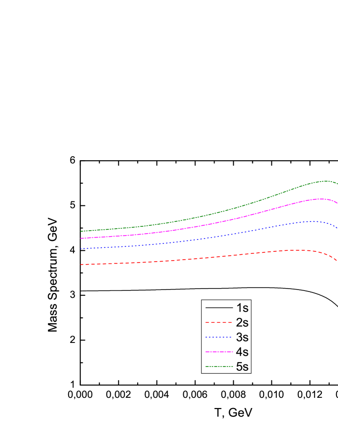
Figure 1: The mass spectrum of charmonium in the $1s$, $2s$, $3s$, $4s$, and $5s$ states as a function of the temperature $T$ with a mass $m_{c}=1.209\,\,\text{GeV}$ and parameters of $A=0.2\,\,\text{GeV}^{2}$, $B=1.244$, and $\delta=0.231\,\,\text{GeV}$.

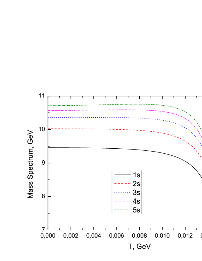
Figure 2: The mass spectrum of bottomonium in the $1s$, $2s$, $3s$, $4s$, and $5s$ states as a function of the temperature $T$ with a mass of $m_{b}=4.823\,\,\text{GeV}$ and parameters of $A=0.2\,\,\text{GeV}^{2}$, $B=1.569$,and $\delta=0.378\,\,\text{GeV}$.

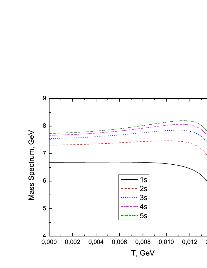
Figure 3: The mass spectrum of $b\overline{c}$ for $1s$, $2s$, $3s$, $4s$, and $5s$ states as a function of the temperature $T$ with masses of $m_{c}=1.209\,\,\text{GeV}$ and $m_{b}=4.823\,\,\text{GeV}$, and parameters of $A=0.2\,\,\text{GeV}^{2}$, $B=1.407$, and $\delta=0.324\,\,\text{GeV}$.

Figure 4: The mass spectrum of charmonium for $1s$, $2s$, $3s$, $4s$, and $5s$ states as a function of the temperature $T$ with a mass of $m_{c}=1.209\,\,\text{GeV}$ and parameters of $A=0.147\,\,\text{GeV}^{2}$, $B=1.204$, $C=2.8\times 10^{-3}$, $D=2.4\times 10^{-5}$, and $\delta=0.379\,\,\text{GeV}$.

Figure 5: The mass spectrum of $bc$ for $1s$, $2s$, $3s$, $4s$, and $5s$ states as a function of the temperature $T$ with a mass of $m_{b}=4.823\,\,\text{GeV}$ and parameters $A=0.147\,\,\text{GeV}^{2}$, $B=1.204$, $C=2.8\times 10^{-3}$, $D=2.4\times 10^{-5}$, and $\delta=0.379\,\,\text{GeV}$.

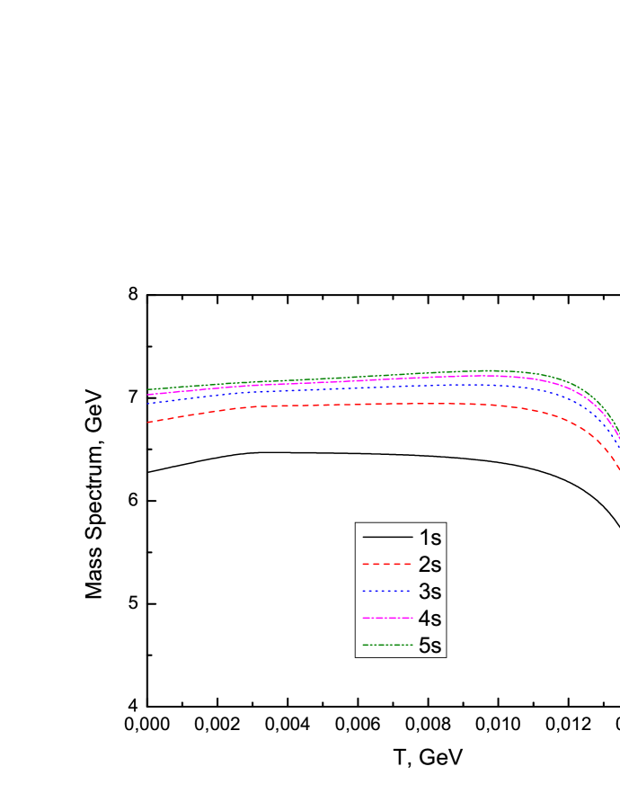
Figure 6: The mass spectrum of $b\overline{c}$ for $1s$, $2s$, $3s$, $4s$, and $5s$ states as a function of the temperature $T$ with masses $m_{c}=1.209\,\,\text{GeV}$, $m_{b}=4.823\,\,\text{GeV}$, and parameters $A=0.147\,\,\text{GeV}^{2}$, $B=1.204$, $C=2.8\times 10^{-3}$, $D=2.4\times 10^{-5}$, and $\delta=0.379\,\,\text{GeV}$.

These results may open new possibilities for determining the properties of the interactions in hadronic system. As a conclusion of the results presented in these tables and figures which are based on analytically results, we may draw the following key points: Firstly, temperature-dependent masses either for the Cornell or the Cornell plus inverse quadratic and harmonic-type potential are very sensitive to the choice of $n_{r}$ radial and $l$ orbital quantum numbers. Secondly, we may consider the temperature-dependent results valid because of the similar shapes between the Cornell and current potentials. These results are sufficiently accurate for practical purposes.

VI Conclusion

The temperature-dependent Schrödinger equation is investigated by applying the NU method . As a potential part of the Schrödinger equation, the Cornell plus inverse quadratic and harmonic oscillator-type is used. Analytical expression for the energy eigenvalues and the radial wave functions is presented. Results are used for describing nonzero and zero temperature mass spectra of heavy quarkonia and $B_{c}$. Numerical results are compared with the experimentally well-established resonances, and some predictions are presented for the states which have not been confirmed yet. For instance, we have the predictions for bottomonium, namely, beside $\Upsilon(1s)$, $\Upsilon(2s)$, $\Upsilon(3s)$, and $\Upsilon(4s)$ resonances, we predict the resonance $\Upsilon(10860)$ and $\Upsilon(11020)$ to be $7s$ and $10s$ states, respectively. For the charmonium states, besides the $J/\psi(1s)$ and $\psi(2s)$ resonances, we predict $3s\longrightarrow\psi(4040)$, $4s\longrightarrow\psi(4260)$, and $5s\longrightarrow\psi(4415)$. We have seen that a zero temperature mass spectrum for $l=0$ is quite in agreement with current experimental data, while for $l\neq 0$, there is some disagreement with experimental data because of the missing spin-spin and spin-orbital momentum interactions terms within the potential. For the temperature- dependent case, we see the strong dependence of the quarkonia mass spectrum on the quantum numbers. Temperature-dependent results for ground states are in good agreement with quantum field theoretical approach such as QCD sum rules results. We have seen that the extension of the Cornell potential leads to slight changes on the masses for nonzero temperature as well as zero temperature.

It seems that this simple potential model, like other nonrelativistic models, is not enough to describe all the features of hadrons within a thermal effect such that having all the hadrons melted at the same temperature contradicts with the lattice data. The most convenient way to compare the prediction of potential models with a direct calculation of quarkonium spectral functions is to calculate the Euclidean meson correlator at finite temperature to compare the lattice data as it was done for the Cornell potential in Mocsy:2004bv ; Mocsy:2005qw . It has been shown that even though potential models with certain screened potentials can reproduce qualitative features of the lattice spectral function, such as the survival of the $1s$ state and the melting of the $1p$ state, the temperature dependence of the meson correlators is not reproduced. According to the lattice results Umeda:2002vr ; Asakawa:2003re the $1s$ charmonium survives up to $1.5T_{c}$ and the $1p$ charmonium dissolves by $1.16T_{c}$ and higher excited states disappear near the transition temperature. It is possible that the effects of the medium on quarkonia binding cannot be understood in a simple potential model. However, one can still do this comparison for other potential models such as the one we have used in this paper. One of the main step for correlator calculation is about the exact solution of the radial Schrödinger equation which is already done in this paper.

The method used in this paper are the systematic ones, and in many cases, it is one of the most concrete works in this area. In particular, the extended Cornell potential can be one of the important potentials, and it deserves special concern in many branches of physics, especially in hadronic, nuclear and atomic physics.

Consequently, studying for an analytical solution of the modified radial Schrödinger equation for the sum of the Cornell, inverse quadratic, and harmonic-type potential within the framework of ordinary quantum mechanics could provide valuable information on the elementary particle physics and quantum chromodynamics and opens new windows for further investigation.

We can conclude that the theoretical results of this study are expected to enable new possibilities for pure theoretical and experimental physicist, because of the exact and more general nature of the results.

Data Availability

The information given in our tables is available for readers in the original references listed in our work.

Conflicts of Interest

The authors declare that they have no conflicts of interest.

Funding

We would like to note that, current research did not receive any specific funding but was performed as part of the employment of the all three authors.

References

- (1) T. Appelquist and H. D. Politzer, ”Heavy quarks and annihilation”, Phys. Rev. Lett. 34, pp.43-45, 1975.
- (2) W. Greiner, Quantum Mechanics. Springer, Berlin, 2001.
- (3) V. G. Bagrov, D. M. Gitman, Exact Solutions of Relativistic Wave Equations (KluwerAcademic Publishers, Dordrecht, 1990)
- (4) L. D. Landau and E. M. Lifshitz, Quantum Mechanics, NonRelativistic Theory. 1977.
- (5) Shi-Hai Dong, Factorization Method in Quantum Mechanics. Springer, Dordrecht, 2007.
- (6) S. M. Kuchin and N. V. Maksimenko, ”Theoretical estimations of the spin averaged mass spectra of heavy quarkonia and bc mesons” Univ. J. Phys. Appl. 1(3): pp.295-298, 2013.
- (7) A. F. Al-Jamel and H. Widyan, ”Heavy quarkonium mass spectra in a Coulomb field plus quadratic potential using Nikiforov-Uvarov method,” Appl. Phys. Res. vol.4, no.3, pp.94-99, 2012.
- (8) N. Maksimenko and S. Kuchin, ”Determination of the mass spectrum of quarkonia by the Nikiforov-Uvarov method,” Russ. Phys. J. 54, no.1, pp.57-65, 2011.
- (9) Z. Ghalenovi, A. A. Rajabi, S. Qin, and D. H. Rischke, ”Ground-state masses and magnetic moments of heavy baryons,” Mod. Phys. Lett. A 29, 1450106, 2014.
- (10) B. J. Vigo-Aguiar and T. E. Simos, ” Review of multistep methods for the numerical solution of the radial Schrödinger equation,” Int. J. Quantum Chem. vol. 103, no.3, pp.278-290, 2005.
- (11) M. Abu-Shady, H. Mansour, and A. I. Ahmadov, ”Dissociation of quarkonium in hot and dense media in an anisotropic plasma in the nonrelativistic quark model,” Adv. High Energy Phys. vol. 2019, Article ID 4785615, 2019.
- (12) H. Karayer, ”Study of the radial Schrödinger equation with external magnetic and AB flux fields by the extended Nikiforov-Uvarov method”, Eur. Phys. J. Plus 135, 70, 2020.
- (13) H. Karayer, D. Demirhan and F. Büyükkılıç, Solution of Schrödinger equation for two different potentials using extended Nikiforov-Uvarov method and polynomial solutions of biconfluent Heun equation,” Journal of Mathematical Physics 59 no. 5, 053501, 2018.
- (14) T. Matsui and H. Satz, ” Suppression by quark-gluon plasma formation,” Phys. Lett. B 178, pp.416-422, 1986.
- (15) F. Karsch, M. Mehr, and H. Satz, ”Color screening and deconfinement for bound states of heavy quarks,” Z. Phys. C 37, 617, 1988.
- (16) M. Abu-Shady, ”N-dimensional Schrödinger equation at finite temperature using the Nikiforov-Uvarov method,” Journal of the Egyptian Mathematical Society 25, pp.86-89, 2017.
- (17) J. Fingberg, ”Heavy quarkonia at high temperature,” Phys. Lett. B 424, pp. 343-354, 1998.
- (18) N. El-Naggar, L. Abou Salem, A. Shalaby, and M. Bourham, ”The equation of state for non-ideal quark gluon plasma,” Phys. Sci. Int. J. 4 no. 7, pp.912-929, 2014.
- (19) G. P. Malik, R. K. Jha, and V. S. Varma, ”Finite-temperature Schrödinger equation: solution in coordinate space,” The Astrophysical Journal, 503, 446, 1998.
- (20) X.-Y. Wu, B.-J. Zhang, X.-J. Liu, Y.-H. Wu, Q.-C. Wang, and Y. Wang, ”Finite temperature Schrödinger equation,” Int. J. Theor. Phys. 50, pp.2546-2551, 2011.
- (21) A. Maireche, ”A theoretical investigation of nonrelativistic bound state solution at finite temperature using the sum of modified Cornell plus inverse quadratic potential,” Sri Lankan Journal of Physics 21 no. 25, pp.11-36, 2020.
- (22) A. Ahmadov, C. Aydin, and O. Uzun, ”Bound state solution of the Schrödinger equation at finite temperature,” J. Phys. Conf. Ser. 1194, no. 1, 012001, 2019.
- (23) M. Abu-Shady and A. Ikot, ”Analytic solution of multi-dimensional Schrödinger equation in hot and dense QCD media using the SUSYQM method,” Eur. Phys. J. Plus 134, no. 7, 321, 2019.
- (24) M. Abu-Shady and A. Ikot, ”Dissociation of nucleon and heavy-baryon in an anisotropic hot and dense QCD medium using Nikiforov-Uvarov method,” Eur. Phys. J. Plus 135, no. 6, 406, 2020.
- (25) W. M. Alberico, A. Beraudo, A. De Pace, and A. Molinari, Quarkonia in the deconfined phase: effective potentials and lattice correlators,” Phys. Rev. D 75, 074009, 2007.
- (26) E. Eichten, K. Gottfried, T. Kinoshita, J. B. Kogut, K. Lane, and T.-M. Yan, ”Spectrum of charmed quark-antiquark bound states,” Phys. Rev. Lett. 34, pp.369-372, 1975.
- (27) E. Eichten, K. Gottfried, T. Kinoshita, K. Lane, and T.-M. Yan, ”Charmonium: the model,” Phys. Rev. D 17, no.11, 3090, 1978.
- (28) R. Rani, S. Bhardwaj, and F. Chand, ”Mass spectra of heavy and light mesons using asymptotic iteration method,” Commun. Theor. Phys. 70, no. 2, 179, 2018.
- (29) M. Abu-Shady, ”Heavy quarkonia and -mesons in the Cornell potential with harmonic oscillator potential in the N-dimensional Schrödinger equation,” APS Physics 2, pp.16-20, 2016.
- (30) A. Vega and J. Flores, ”Heavy quarkonium properties from Cornell potential using variational method and supersymmetric quantum mechanics”, Pramana 87, 73, 2016.
- (31) E. Khokha, M. Abu-Shady, and T. Abdel-Karim, ”Quarkonium masses in the N-dimensional space using the analytical exact iteration method”, International Journal of Theoretical and Applied Mathematics, vol.2, no.2,pp. 86-92, 2016.
- (32) M. Abu-Shady, T. Abdel-Karim, and S. Y. Ezz-Alarab, ”Masses and thermodynamics properties of heavy mesons in the non-relativistic quark model using Nikiforov-Uvarov meethod”, J. Egyptian Math. Soc. 27, 14, 2019.
- (33) H. Mansour and A. Gamal, Bound state of heavy quarks using a general polynomial potential,” Adv. High Energy Phys. vol. 2018, Article ID 7269657, 2018.
- (34) M. Abu-Shady, T. Abdel-Karim, and E. Khokha, ”Exact solution of the -dimensional radial Schrödinger equation via Laplace transformation method with the generalized Cornell potential”, SciFed Journal of Quantum Physics, vol.2, no.1, pp.1-11, 2018.
- (35) S. Hassanabadi, A. Rajabi, and S. Zarrinkamar, ”Cornell and Kratzer potentials within the semirelativistic treatment”, Mod. Phys. Lett. A 27, 1250057, 2012.
- (36) A. N. Ikot, G. J. Rampho, P. O. Amadi, U. S. Okorie, M. J. Sithole, and M. L. Lekala, ”Quantum information-entropic measures for exponential-type potential,” Results in Physics, 18, 103150, 2020.
- (37) Shi-Hai Dong, Guo-Hua Sun, and M. Lozada-Cassou, ”Exact solutions and ladder operators for a new anharmonic oscillator,” Physics Letters A. 340, 94, 2005.
- (38) Xiao-Hua Wang, Shi-Hai Dong, Chang-Yuan Chen, and Yuan You, ”Exact solutions of the Schrödinger equation with double ring-shaped oscillator,” Physics Letters A. 377, 1521, 2013.
- (39) Qian Dong, H.Ivnán Garcia Hernández, Guo-Hua Sun, Mohamad Toutounji, and Shi-Hai Dong, ”Exact solutions of the harmonic oscillator plus non-polynomial interaction,” Proc. R. Soc. A 476, 20200050, 2020.
- (40) Xi-Wen Hou, Shi-Hai Dong, and Zhong-Qi Ma, ”Relativistic levinson theorem in two Dimensions,” Phys. Rev. A. 58, no. 3, 2160, 1998.
- (41) A. F. Nikiforov and V. B. Uvarov, Special Functions of Mathematical Physics, Birkhäuser, Basel 1988.
- (42) C. Pekeris, ”The rotation-vibration coupling in diatomic molecules,” Phys. Rev. 45, pp.98-103, 1934.
- (43) E. Omugbe, O. E. Osafile, and M. C. Onyeaju, Mass spectrum of mesons via the WKB approximation method,” Adv. High Energy Phys., vol.2020, Article ID 5901464, 2020.
- (44) P.A. Zyla et al. (Particle Data Group), Prog. Theor. Exp. Phys. 2020, 083C01 (2020).
- (45) R. N. Faustov, V. O. Galkin, A. V. Tatarintsev, and A. S. Vshivtsev, ”Spectral problem of the radial Schrödinger equation with confining power potentials,” Theor. Math. Phys. 113, pp.1530-1542, 1997.
- (46) R. Kumar and F. Chand, ”Series solutions to the N-dimensional radial Schrödinger equation for the quark-antiquark interaction potential,” Phys. Scr. 85, 055008, 2012.
- (47) G. Boyd, J. Engels, F. Karsch, E. Laermann, C. Legeland, M. Lutgemeier, and B. Petersson, ”Thermodynamics of SU(3) lattice gauge theory,” Nucl. Phys. B 469, pp.419-444, 1996.
- (48) C. Bernard, T. Burch, E. Gregory et al., ”QCD thermodynamics with three flavors of improved staggered quarks,” Phys. Rev. D 71, 034504, 2005.
- (49) E. Veliev, H. Sundu, K. Azizi, and M. Bayar, ”Scalar quarkonia at finite temperature,” Phys. Rev. D 82, 056012, 2010.
- (50) Á. Mócsy and P. Petreczky, ”Heavy quarkonia survival in potential model,” Eur. Phys. J. C 43, pp. 77-80, 2005.
- (51) Á. Mócsy and P. Petreczky, ”Quarkonia correlators above deconfinement,” Phys. Rev. D 73, 074007, 2006.
- (52) T. Umeda, K. Nomura, and H. Matsufuru, ”Charmonium at finite temperature in quenched lattice QCD,” Eur. Phys. J. C 39S1, pp. 9-26, 2005.
- (53) M. Asakawa and T. Hatsuda, and in the deconfined plasma from lattice QCD, Phys. Rev. Lett. 92, 012001, 2004.