Coordinate descent heuristics for the irregular strip packing problem of rasterized shapes

Abstract

We consider the irregular strip packing problem of rasterized shapes, where a given set of pieces of irregular shapes represented in pixels should be placed into a rectangular container without overlap. The rasterized shapes provide simple procedures of the intersection test without any exceptional handling due to geometric issues, while they often require much memory and computational effort in high-resolution. To reduce the complexity of rasterized shapes, we propose a pair of scanlines representation called the double scanline representation that merges consecutive pixels in each row and column into strips with unit width, respectively. Based on this, we develop coordinate descent heuristics for the raster model that repeat a line search in the horizontal and vertical directions alternately, where we also introduce a corner detection technique used in computer vision to reduce the search space. Computational results for test instances show that the proposed algorithm obtains sufficiently dense layouts of rasterized shapes in high-resolution within a reasonable computation time.

1 Introduction

The irregular strip packing problem (ISP), or often called the nesting problem, is the one of the representative cutting and packing problems that emerges in a wide variety of industrial applications, such as garment manufacturing, sheet metal cutting, furniture making and shoe manufacturing [Alvarez-Valdes et al., 2018, Scheithauer, 2018]. This problem is categorized as the two-dimensional, irregular open dimensional problem in Dyckhoff [1990], Wäscher et al. [2007]. Given a set of pieces of irregular shapes and a rectangular container with a fixed width and a variable length, this problem asks a feasible layout of the pieces into the container such that no pair of pieces overlaps with each other and the container length is minimized. We note that rotations of pieces are usually restricted to a few number of degrees (e.g., 0 or 180 degrees) in many industrial applications, because textiles have grain and may have a drawing pattern. Figure 1 shows an instance of ISP and a feasible solution.

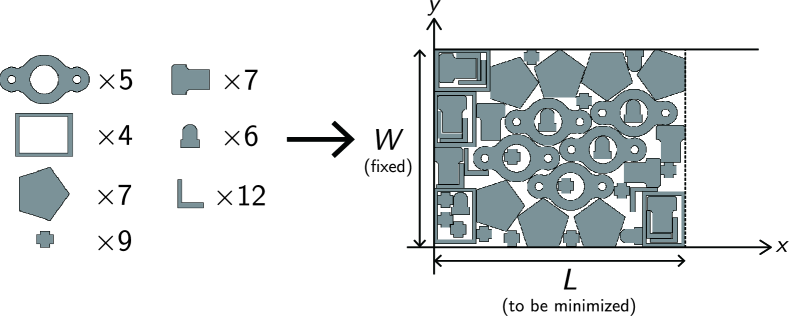
Figure 1: An instance of the irregular strip packing problem and its solution.

The first issue encountered when handling ISP is how to represent the irregular shapes. In computer graphics, the irregular shapes are often represented in two models as shown in Figure 2: the vector model represents an irregular shape as a set of chained line and curve segments forming its outline, and the raster model (also known as the bitmap model) represents an irregular shape as a set of grid pixels forming its inside.

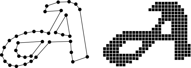
Figure 2: The vector and raster representations for an irregular shape.

The vector model requires complicated trigonometric computations with many exception handling for the intersection test of the irregular shapes, while the raster model provides simple computations without any exception handling. On the other hand, the vector model often consumes less memory usage and computation time for the intersection test than the raster model, because the number of line and curve segments in the vector model often becomes much smaller than that of grid pixels in the raster model.

For the vector model, in particular polygons, the recent development of computational geometry such as the no-fit polygon (NFP) enables us to compute their intersection test efficiently [Bennell & Oliveira, 2008, Leao et al., 2020]. Based on the efficient geometric computations, many efficient heuristic algorithms have been developed for ISP of the polygons (called the polygon packing problem in this paper) [Bennell & Oliveira, 2009, Hu et al., 2018b]. A standard approach for the polygon packing problem is to develop construction algorithms, e.g., the bottom-left (BL) algorithm and the bottom-left fill (BLF) algorithm that places the pieces one by one into the container based on a given order [Albano & Sapuppo, 1980, Błȧzewicz et al., 1993, Oliveira et al., 2000, Dowsland et al., 2002, Gomes & Oliveira, 2002, Bennell & Song, 2010]. Another approach is to resort improvement algorithms that relocate pieces by solving the compaction problem and/or the separation problem [Li & Milenkovic, 1995, Bennell & Dowsland, 2001, Gomes & Oliveira, 2006]. The compaction problem relocates pieces from a given feasible placement so as to minimize the container length. The separation problem relocates pieces from a given infeasible placement so as to make it feasible while minimizing the total amount of their translation. The overlap minimization problem (OMP) is a variant of the separation problem that places pieces within the container with given width and length so as to minimize the overlap penalty for all pairs of pieces [Egeblad et al., 2007, Imamichi et al., 2009, Umetani et al., 2009, Leung et al., 2012, Elkeran, 2013].

Mundim et al. [2017] and Sato et al. [2019] constrained the search space to place the pieces on a discrete set of positions (i.e., a grid), and developed a discretized NFP called the no-fit raster for the intersection test of the irregular shapes. This constrained model of the search space on a grid is called the dotted-board model [Toledo et al., 2013], which is similar to the raster model but different because the given pieces are represented in polygons (i.e., the vector model).

For the raster model, Oliveira & Ferreira [1993], Segenreich & Braga [1986] and Babu & Babu [2001] represented the pieces by matrices of different codes [Bennell & Oliveira, 2008]. The raster representations are simple to code the irregular shapes and provide simple procedures for their intersection test, which enable us to develop practical software for a wide variety of free-form packing problems including many curve segments and holes only by converting input data to pixels. However, their computational costs highly depend on the resolution of the raster representations; i.e., improving the resolution much increases the memory usage and computation time for the procedures. To improve the computational efficiency of the intersection test and the overlap minimization for the raster model, Okano [2002] and Hu et al. [2018a] proposed sophisticated data structures that merge the pixels of the irregular shapes into strips or rectangles. Using these representations, several heuristic algorithms have been developed for ISP of the raster model [Segenreich & Braga, 1986, Oliveira & Ferreira, 1993, Jain & Gea, 1998, Babu & Babu, 2001, Chen et al., 2004, Wong et al., 2009]. Despite these heuristic algorithms for the raster model, their computational results were still restricted for the instances of low-resolution and insufficient to convince their high performance for the instances of high-resolution.

In this paper, we develop an efficient line search algorithm for coordinate descent heuristics in the raster model, which makes it possible to high performance improvement algorithms for the instances of high-resolution. The coordinate descent heuristics (CDH) is one of improvement algorithms that repeat a line search in the horizontal and vertical directions alternately, which have achieved high performance for ISP of the vector model [Egeblad et al., 2007, Umetani et al., 2009]. However, unlike the vector model, the conventional raster representations were computationally much expensive to develop any efficient line search algorithms especially in high-resolution. To reduce the complexity of rasterized shapes, we propose a pair of scanlines representation called the double scanline representation for NFPs of the rasterized shapes that reduces their complexity by merging consecutive pixels in each row and column into strips with unit width, respectively. We also introduce a corner detection technique used in computer vision [Rosten & Drummond, 2006] to reduce the search space of the line search. The coordinate descent heuristics are incorporated into a variant of the guided local search (GLS) for OMP based on Umetani et al. [2009]. Using this as a main component, we then develop a heuristic algorithm for ISP, which we call the guided coordinate descent heuristics (GCDH).

This paper is organized as follows. We first formulate ISP and OMP in the raster model and illustrate the outline of the proposed algorithm GCDH for ISP in Section 2. We then introduce an efficient intersection test for rasterized shapes in Section 3. We explain the main component of the proposed algorithm CDH for OMP in Section 4 and the construction algorithm for an initial solution of ISP in Section 5. Finally, we report computational results in Section 6 and make concluding remarks in Section 7.

2 Formulation and approach

2.1 Irregular strip packing problem of rasterized shapes

We are given a list of $n$ pieces $\mathcal{P}=\{P_{1},P_{2},\dots,P_{n}\}$ of rasterized shape with a list of their possible orientations $\mathcal{O}=(O_{1},O_{2},\dots,O_{n})$, where a piece $P_{i}$ can be rotated by $o$ degrees for each $o\in O_{i}$. We assume without loss of generality that zero degree is always included in $O_{i}$. We are also given a rectangular container $C=C(W,L)$ with a width $W$ and a length $L$, where $W$ is a non-negative constant and $L$ is a non-negative variable. We assume that the container edges with the width $W$ and the length $L$ are parallel to the $y$-axis and the $x$-axis as shown in Figure 1, respectively, and the bottom-left corner of the container $C$ is the origin $(0,0)$. We denote $P_{i}(o)$ as a piece $P_{i}$ rotated by $o\in O_{i}$ degrees, which may be written as $P_{i}$ for simplicity when its orientation is not specified or clear from the context. We consider the bounding-box of a piece $P_{i}(o)$ as the smallest rectangle that encloses $P_{i}(o)$, and its width and length are denoted by $w_{i}(o)$ and $l_{i}(o)$, respectively. We describe a position of a piece $P_{i}(o)$ by a coordinate $\bm{v}_{i}=(x_{i},y_{i})$ of the center of its bounding box called the reference point. For convenience, we regard a piece $P_{i}$ as a set of grid pixels when its reference point is put at the origin $(0,0)$ and a rotated piece $P_{i}(o)$ is sometimes reshaped to fit grid pixels. We then describe a piece $P_{i}$ placed at $\bm{v}_{i}$ by the Minkowski sum

$$P_{i}\oplus\bm{v}_{i}=\{\bm{p}+\bm{v}_{i}\mid\bm{p}\in P_{i}\}.$$ (1)

We describe a solution of ISP by lists of positions $\bm{v}=(\bm{v}_{1},\bm{v}_{2},\dots,\bm{v}_{n})$ and orientations $\bm{o}=(o_{1},o_{2},\dots,o_{n})$ of all pieces $P_{i}$ ($i=1,\dots,n$). We note that a solution $(\bm{v},\bm{o})$ uniquely determines a layout of the pieces. The ISP is described as follows:

$$\begin{array}[]{llll}(\textnormal{ISP})&\textnormal{minimize}&L\\ &\textnormal{subject to}&\lfloor l_{i}(o_{i})/2\rfloor\leq x_{i}\leq L-\lfloor l_{i}(o_{i})/2\rfloor,&1\leq i\leq n,\\ &&\lfloor w_{i}(o_{i})/2\rfloor\leq y_{i}\leq W-\lfloor w_{i}(o_{i})/2\rfloor,&1\leq i\leq n,\\ &&(P_{i}(o_{i})\oplus\bm{v}_{i})\cap(P_{j}(o_{j})\oplus\bm{v}_{j})=\emptyset,&1\leq i<j\leq n,\\ &&L\in\mathbb{Z}_{+},\\ &&\bm{v}_{i}=(x_{i},y_{i})\in\mathbb{Z}_{+}^{2},&1\leq i\leq n,\\ &&o_{i}\in O_{i},&1\leq i\leq n,\end{array}$$ (2)

where $\mathbb{Z}_{+}$ is the set of nonnegative integer values. We note that the coordinate $\bm{v}_{i}=(x_{i},y_{i})$ of a piece $P_{i}(o_{i})$ takes $(\lfloor l_{i}(o_{i})/2\rfloor,\lfloor w_{i}(o_{i})/2\rfloor)$ and $(L-\lfloor l_{i}(o_{i})/2\rfloor,W-\lfloor w_{i}(o_{i})/2\rfloor)$ when it is placed at the bottom-left and top-right corners of the container $C$, respectively. We also note that minimization of the length $L$ is equivalent to maximization of the density defined by $\sum_{1\leq i\leq n}(\textnormal{area of}\;P_{i})/WL$.

2.2 Overlap minimization problem

We consider OMP as a sub-problem of ISP to find a feasible layout $(\bm{v},\bm{o})$ of given pieces for the container $C$ with a given length $L$. A solution of OMP may have a number of overlapping pieces, and the total amount of overlap is penalized in such a way that a solution with no penalty gives a feasible layout for ISP. Let $f_{ij}(\bm{v}_{i},\bm{v}_{j},o_{i},o_{j})$ be a function that measures the overlap amount for a pair of pieces $P_{i}(o_{i})\oplus\bm{v}_{i}$ and $P_{j}(o_{j})\oplus\bm{v}_{j}$. The objective of OMP is to find a solution $(\bm{v},\bm{o})$ that minimizes the total amount of the overlap penalty $F(\bm{v},\bm{o})=\sum_{1\leq i<j\leq n}f_{ij}(\bm{v}_{i},\bm{v}_{j},o_{i},o_{j})$ under the constraint that all pieces $P_{i}$ ($1\leq i\leq n$) are placed within the container $C(W,L)$.

$$\begin{array}[]{llll}(\textnormal{OMP})&\textnormal{minimize}&F(\bm{v},\bm{o})=\displaystyle\sum_{1\leq i<j\leq n}f_{ij}(\bm{v}_{i},\bm{v}_{j},o_{i},o_{j})\\ &\textnormal{subject to}&\lfloor l_{i}(o_{i})/2\rfloor\leq x_{i}\leq L-\lfloor l_{i}(o_{i})/2\rfloor,&1\leq i\leq n,\\ &&\lfloor w_{i}(o_{i})/2\rfloor\leq y_{i}\leq W-\lfloor w_{i}(o_{i})/2\rfloor,&1\leq i\leq n,\\ &&\bm{v}_{i}=(x_{i},y_{i})\in\mathbb{Z}_{+}^{2},&1\leq i\leq n,\\ &&o_{i}\in O_{i},&1\leq i\leq n.\end{array}$$ (3)

We introduce the directional penetration depth to define the overlap penalty function $f_{ij}(\bm{v}_{i},\bm{v}_{j},o_{i},o_{j})$ for a pair of pieces $P_{i}(o_{i})\oplus\bm{v}_{i}$ and $P_{j}(o_{j})\oplus\bm{v}_{j}$, which was originally defined as the minimum translational distance in a given direction to separate a pair of polygons [Dobkin et al., 1993]. If they do not overlap, then their directional penetration depth is zero. In the raster model, we define the directional penetration depth in the horizontal and vertical directions as follows:

$$\delta(P_{i},P_{j},\bm{d})=\min\{|t|\mid P_{i}\cap(P_{j}\oplus t\bm{d})=\emptyset,t\in\mathbb{Z}\},\;\;\bm{d}\in\{(1,0),(0,1)\}.$$ (4)

We then define the overlap penalty $f_{ij}(\bm{v}_{i},\bm{v}_{j},o_{i},o_{j})$ for a pair of pieces $P_{i}(o_{i})\oplus\bm{v}_{i}$ and $P_{j}(o_{j})\oplus\bm{v}_{j}$ as the minimum within the horizontal and vertical penetration depths

$$f_{ij}(\bm{v}_{i},\bm{v}_{j},o_{i},o_{j})=\min\{\delta(P_{i}(o_{i})\oplus\bm{v}_{i},P_{j}(o_{j})\oplus\bm{v}_{j},\bm{d})\mid\bm{d}\in\{(1,0),(0,1)\}\}.$$ (5)

2.3 Entire algorithm for the irregular strip packing problem

We give an entire description of the proposed algorithm GCDH for ISP. The GCDH first generates an initial solution $(\bm{v},\bm{o})$ by a construction algorithm to be explained in Section 5, and sets the minimum container length $L$ containing all pieces $P_{i}$ ($1\leq i\leq n$). It then searches the minimum feasible container length $L^{\ast}$ by shrinking or extending the right sides of the container $C$ until the time limit is reached, where the ratios of shrinking and extending container length are controlled by the parameters $r_{\mathrm{dec}}$ and $r_{\mathrm{inc}}$, respectively. If the current solution $(\bm{v},\bm{o})$ is feasible, then it shrinks the container length $L$ to $\lfloor(1-r_{\mathrm{dec}})L\rfloor$ and relocates protruding pieces $P_{i}$ at random positions in the container $C(W,L)$; otherwise it extends the container length $L$ to $\lfloor(1+r_{\mathrm{inc}})L\rfloor$. If there is at least one overlapping pair of pieces in the current solution, then it tries to resolve overlap by CDH for OMP explained in Section 4. Figure 3 shows the outline of the proposed algorithm GCDH.

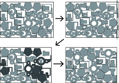
Figure 3: The outline of the proposed algorithm (GCDH).

The algorithm is formally described in Algorithm 1, where we omit the input data $W,\mathcal{P},\mathcal{O}$ commonly used in all algorithms in this paper.

Algorithm 1 GCDH

1:

2:$L,(\bm{v},\bm{o})\leftarrow\textnormal{{\sc Construct}}$ {See Algorithm 5}

3:$L^{\ast}\leftarrow L$, $(\bm{v}^{\ast},\bm{o}^{\ast})\leftarrow(\bm{v},\bm{o})$

4:$L\leftarrow\lfloor(1-r_{\mathrm{dec}})L^{\ast}\rfloor$

5:repeat

6:    $(\bm{v},\bm{o})\leftarrow\textnormal{GLS}(L,\bm{v},\bm{o})$ {See Algorithm 4}

7:    if $(\bm{v},\bm{o})$ is feasible then

8:         $L^{\ast}\leftarrow L$, $(\bm{v}^{\ast},\bm{o}^{\ast})\leftarrow(\bm{v},\bm{o})$

9:         $L\leftarrow\lfloor(1-r_{\mathrm{dec}})L^{\ast}\rfloor$

10:         Relocate protruding pieces $P_{i}(o_{i})$ at random position in $C(W,L)$.

11:    else

12:         $L\leftarrow\lfloor(1+r_{\mathrm{inc}})L\rfloor$

13:         if $L\geq L^{\ast}$ then

14:             $L\leftarrow\lfloor(1-r_{\mathrm{dec}})L^{\ast}\rfloor$, $(\bm{v},\bm{o})\leftarrow(\bm{v}^{\ast},\bm{o}^{\ast})$

15:             Relocate protruding pieces $P_{i}(o_{i})$ at random position in $C(W,L)$.              

16:until The time limit is reached

17:Return $(\bm{v}^{\ast},\bm{o}^{\ast})$

3 Intersection test for rasterized shapes via scanline representation

3.1 No-fit polygon for intersection test

The no-fit polygon (NFP) introduced by Art [1966] is a representative geometric technique used in many algorithms for the polygon packing problem. It is also used for other applications such as image processing and robot motion planning, and is also known as the Minkowski difference and the configuration-space obstacle, respectively. The no-fit polygon $\mathrm{NFP}(P_{i},P_{j})$ of an ordered pair of pieces $P_{i}$ and $P_{j}$ is defined by

$$\mathrm{NFP}(P_{i},P_{j})=P_{i}\oplus(-P_{j})=\{\bm{u}-\bm{w}\mid\bm{u}\in P_{i},\bm{w}\in P_{j}\}.$$ (6)

The NFP has an important property that $P_{j}\oplus\bm{v}_{j}$ overlaps with $P_{i}\oplus\bm{v}_{i}$ if and only if $\bm{v}_{j}-\bm{v}_{i}\in\mathrm{NFP}(P_{i},P_{j})$ holds. That is, the intersection test for two irregular shapes $P_{i}\oplus\bm{v}_{i}$ and $P_{j}\oplus\bm{v}_{j}$ can be identified by testing whether a point $\bm{v}_{j}-\bm{v}_{i}$ is inside an irregular shape $\mathrm{NFP}(P_{i},P_{j})$ or not. Figure 4 shows an example of $\mathrm{NFP}(P_{i},P_{j})$ for two irregular shapes $P_{i}$ and $P_{j}$, where the solid arrow illustrates the minimum translation of the piece $P_{j}$ to separate from the piece $P_{i}$ within the horizontal and vertical directions. The NFP enables us to compute the intersection test and the directed penetration depth efficiently, assuming that we compute NFPs for all pairs of pieces in advance.

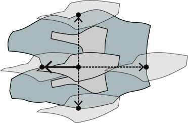
Figure 4: The no-fit polygon $\mathrm{NFP}(P_{i},P_{j})$ for two irregular shapes $P_{i}$ and $P_{j}$.

3.2 Scanline representation for rasterized shapes

We consider a pair of scanlines representation called the double scanline representation that reduces the complexity of rasterized shapes by merging consecutive pixels in each row and column into strips with unit width, respectively. Figure 5 shows an example of the double scanline representation of a rasterized shape.

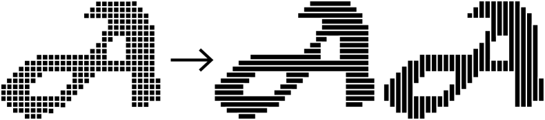
Figure 5: The double scanline representation for a rasterized shape.

Hu et al. [2018a] developed an efficient algorithm to compute NFPs of a single (i.e., horizontal or vertical) scanline representation called the Integrate-NFP (See details of its implementation in Hu et al. [2018a]).

Based on this, we compute the horizontal penetration depth $\delta(P_{i}\oplus\bm{v}_{i},P_{j}\oplus\bm{v}_{j},(1,0))$ efficiently. Figure 6 shows an example of computing the horizontal (and vertical) penetration depth from NFP of the scanline representation.

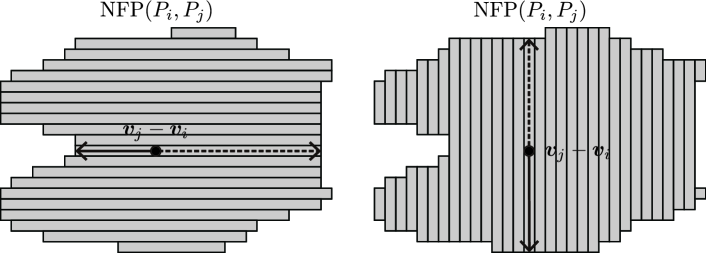
Figure 6: Computing the horizontal and vertical penetration depths from the scanline representations of NFP.

Let $\mathcal{S}_{ij}=\{S_{ij1},S_{ij2},\dots,S_{ijm_{ij}}\}$ be the set of horizontal strips representing $\mathrm{NFP}(P_{i},P_{j})$, where $m_{ij}$ is the number of strips representing $\mathrm{NFP}(P_{i},P_{j})$. When the relative position $\bm{v}_{j}-\bm{v}_{i}$ of the piece $P_{j}$ is placed in a strip $S_{ijk}$, the horizontal penetration depth $\delta(P_{i}\oplus\bm{v}_{i},P_{j}\oplus\bm{v}_{j},(1,0))$ then takes the minimum length from $\bm{v}_{j}-\bm{v}_{i}$ to left and right side of the strip $S_{ijk}$. We note that the horizontal penetration depth can be computed in $\mathrm{O}(1)$ time when $\mathrm{NFP}(P_{i},P_{j})$ is $y$-monotone, where a rasterized shape is $y$-monotone if it can be represented by a set of strips such that there is exactly one strip for each row and strips in adjacent rows are contiguous. We also compute the vertical penetration depth $\delta(P_{i}\oplus\bm{v}_{i},P_{j}\oplus\bm{v}_{j},(0,1))$ efficiently utilizing the vertical scanline representation of $\mathrm{NFP}(P_{i},P_{j})$ in the same fashion. In Figure 6, the solid arrows illustrate the minimum translation of the piece $P_{j}$ to separate from the piece $P_{i}$ in the horizontal and vertical directions, and their lengths are the horizontal and vertical penetration depths, respectively.

4 Coordinate descent heuristics for the overlap minimization problem

4.1 Outline of the coordinate descent heuristics

We develop an improvement algorithm for OMP called the coordinate descent heuristics (CDH), which start from an initial solution and repeatedly apply the line search that minimizes the objective function along a coordinate direction until no better solution is found in any coordinate directions.

We first explain the neighborhood of the CDH for OMP. Let $(\bm{v},\bm{o})$ be the current solution. The neighborhood $\mathrm{NB}(\bm{v},\bm{o})$ is defined as the set of neighbor solutions, where a neighbor solution $(\bm{v}^{\prime},\bm{o}^{\prime})\in\mathrm{NB}(\bm{v},\bm{o})$ is obtained by setting a new orientation $o_{k}^{\prime}\in O_{k}$ of a piece $P_{k}$ ($1\leq k\leq n$) and iteratively applying the line search to find a new position $\bm{v}_{k}^{\prime}$. The quality of a solution $(\bm{v},\bm{o})$ is measured by the following weighted overlap penalty function

$$\widetilde{F}(\bm{v},\bm{o})=\sum_{1\leq i<j\leq n}\alpha_{ij}\cdot f_{ij}(\bm{v}_{i},\bm{v}_{j},o_{i},o_{j}),$$ (7)

where $\alpha_{ij}>0$ are the penalty weights and $f_{ij}$ are the overlap penalties defined in (5) for a pair of pieces $P_{i}(o_{i})\oplus\bm{v}_{i}$ and $P_{j}(o_{j})\oplus\bm{v}_{j}$. The penalty weights $\alpha_{ij}$ are adaptively controlled by GLS to be explained in Section 4.3. For a piece $P_{k}(o_{k}^{\prime})$, the neighborhood search finds a new position $\bm{v}_{k}^{\prime}$ in the container $C(W,L)$ such that the following weighted overlap penalty function

$$\widetilde{F}_{k}(\bm{v}_{k}^{\prime},o_{k}^{\prime})=\sum_{1\leq j\leq n,j\not=k}\alpha_{kj}\cdot f_{kj}(\bm{v}_{k}^{\prime},\bm{v}_{j},o_{k}^{\prime},o_{j})$$ (8)

is minimized. For this, the neighborhood search repeatedly moves the piece $P_{k}(o_{k}^{\prime})$ in the horizontal and vertical directions alternately until no better position is found in either direction. Figure 7 shows how the neighborhood search proceeds.

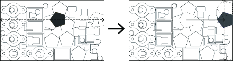
Figure 7: The neighborhood search of CDH for OMP.

For each move of the piece $P_{k}(o_{k}^{\prime})$ in a specified direction $\bm{d}\in\{(1,0),(0,1)\}$, let

$$N=\{t\mid P(o_{k}^{\prime})\oplus(\bm{v}_{k}+t\bm{d})\subseteq C(W,L),t\in\mathbb{Z}\}$$ (9)

be the set of valid $t$ such that the piece $P_{k}(o_{k}^{\prime})$ placed on the line $\bm{v}_{k}+t\bm{d}$ ($t\in\mathbb{Z}$) is contained in the container $C(W,L)$, where $\mathbb{Z}$ is the set of integer values. The line search (to be explained in Section 4.2) finds a new valid position $\bm{v}_{k}^{\prime}=\bm{v}_{k}+t\bm{d}$ ($t\in N$) that minimizes the weighted overlap penalty function $\widetilde{F}_{k}(\bm{v}_{k}+t\bm{d},o_{k}^{\prime})$. The neighborhood search is formally described in Algorithm 2.

Algorithm 2 NeighborSearch($L,\bm{v},\bm{o},P_{k},o_{k}^{\prime}$)

1:

2:$\bm{v}^{\prime}\leftarrow\bm{v}$, $o_{j}^{\prime}\leftarrow o_{j}$ ($j\not=k$), $\bm{d}\leftarrow(1,0)$

3:Find $t\in N$ to minimize $\widetilde{F}_{k}(\bm{v}_{k}^{\prime}+t\bm{d},o_{k}^{\prime})$

4:if $\widetilde{F}_{k}(\bm{v}_{k}^{\prime}+t\bm{d},o_{k}^{\prime})<\widetilde{F}_{k}(\bm{v}_{k}^{\prime},o_{k}^{\prime})$ then

5:    $\bm{v}_{k}^{\prime}\leftarrow\bm{v}_{k}^{\prime}+t\bm{d}$

6:$\bm{d}\leftarrow(0,1)$

7:repeat

8:    Find $t\in N$ to minimize $\widetilde{F}_{k}(\bm{v}_{k}^{\prime}+t\bm{d},o_{k}^{\prime})$

9:    if $\widetilde{F}_{k}(\bm{v}_{k}^{\prime}+t\bm{d},o_{k}^{\prime})<\widetilde{F}_{k}(\bm{v}_{k}^{\prime},o_{k}^{\prime})$ then

10:         $\bm{v}_{k}^{\prime}\leftarrow\bm{v}_{k}^{\prime}+t\bm{d}$     

11:    if $\bm{d}=(1,0)$ then

12:         $\bm{d}\leftarrow(0,1)$

13:    else

14:         $\bm{d}\leftarrow(1,0)$     

15:until $\widetilde{F}_{k}(\bm{v}_{k}^{\prime}+t\bm{d},o_{k}^{\prime})=\widetilde{F}_{k}(\bm{v}_{k}^{\prime},o_{k}^{\prime})$

16:Return $(\bm{v}^{\prime},\bm{o}^{\prime})$

We now describe the outline of CDH for OMP. Starting from an initial solution $(\bm{v},\bm{o})$ with some overlapping pieces, CDH repeatedly replaces the current solution $(\bm{v},\bm{o})$ with the first improved solution $(\bm{v}^{\prime},\bm{o}^{\prime})\in\mathrm{NB}(\bm{v},\bm{o})$ obtained by the neighborhood search. That is, CDH searches $\mathrm{NB}(\bm{v},\bm{o})$ in random order, and if it finds an improved solution $(\bm{v}^{\prime},\bm{o}^{\prime})\in\mathrm{NB}(\bm{v},\bm{o})$ satisfying $\widetilde{F}(\bm{v}^{\prime},\bm{o}^{\prime})<\widetilde{F}(\bm{v},\bm{o})$, then it immediately replaces the current solution $(\bm{v},\bm{o})$ with $(\bm{v}^{\prime},\bm{o}^{\prime})$. If no overlapping piece exists in the current solution $(\bm{v},\bm{o})$ (i.e., $\widetilde{F}(\bm{v},\bm{o})=0$) or no better solution found in $\mathrm{NB}(\bm{v},\bm{o})$, then CDH outputs $(\bm{v},\bm{o})$ as a locally optimal solution and the best solution $(\bm{v}^{\ast},\bm{o}^{\ast})$ obtained so far, measured by the original penalty function $F$, and halts.

We also incorporate the fast local search (FLS) strategy [Voudouris & Tsang, 1999] to improve the efficiency of CDH. The strategy decomposes the neighborhood into a number of subneighborhoods, which are labeled active or inactive depending on whether they are being searched or not, i.e., it skips evaluating all neighbor solutions in inactive subneighborhoods. We define the subneighborhood $\mathrm{NB}_{k}(\bm{v},\bm{o})$ ($1\leq k\leq n$) of the current solution $(\bm{v},\bm{o})$ as the set of solutions obtainable by setting orientation $o_{k}^{\prime}\in O_{k}$ and applying the neighborhood search to the piece $P_{k}$, i.e., the neighborhood $\mathrm{NB}(\bm{v},\bm{o})$ is partitioned with respect to the pieces $P_{k}$ ($1\leq k\leq n$). The CDH first sets all subneighborhoods $\mathrm{NB}_{k}(\bm{v},\bm{o})$ ($1\leq k\leq n$) to be active, and it searches active subneighborhoods $\mathrm{NB}_{k}(\bm{v},\bm{o})$ in random order. If no improvement has been made in an active subneighborhood $\mathrm{NB}_{k}(\bm{v},\bm{o})$, then CDH inactivates it. If CDH finds an improved solution $(\bm{v}^{\prime},\bm{o}^{\prime})$ satisfying $\widetilde{F}(\bm{v}^{\prime},\bm{o}^{\prime})<\widetilde{F}(\bm{v},\bm{o})$ in an active subneighborhood $\mathrm{NB}_{k}(\bm{v},\bm{o})$, then it activates all subneighborhood $\mathrm{NB}_{j}(\bm{v},\bm{o})$ corresponding to the pieces $P_{j}$ overlapping with the piece $P_{k}$ before and after its move. The CDH is formally described in Algorithm 3, where $A$ denotes the set of indices $k$ ($1\leq k\leq n$) corresponding to the active subneighborhood $\mathrm{NB}_{k}(\bm{v},\bm{o})$, and $(\bm{v}^{\ast},\bm{o}^{\ast})$ and $(\tilde{\bm{v}},\tilde{\bm{o}})$ denote the best solutions of the original overlap penalty function $F$ and the weighted overlap penalty function $\widetilde{F}$, respectively.

Algorithm 3 CDH($L,\bm{v},\bm{o}$)

1:

2:$(\tilde{\bm{v}},\tilde{\bm{o}})\leftarrow(\bm{v},\bm{o})$, $(\bm{v}^{\ast},\bm{o}^{\ast})\leftarrow(\bm{v},\bm{o})$, $A\leftarrow\{1,\dots,n\}$

3:while $A\not=\emptyset$ do

4:    Randomly select $k\in A$

5:    $O\leftarrow O_{k}$

6:    while $O\not=\emptyset$ do

7:         Randomly select $o_{k}^{\prime}\in O$

8:         $(\bm{v}^{\prime},\bm{o}^{\prime})\leftarrow\textnormal{{\sc NeighborSearch}}(L,\bm{v},\bm{o},P_{k},o_{k}^{\prime})$ {See Algorithm 2}

9:         if $F(\bm{v}^{\prime},\bm{o}^{\prime})<F(\bm{v}^{\ast},\bm{o}^{\ast})$ then

10:             $(\bm{v}^{\ast},\bm{o}^{\ast})\leftarrow(\bm{v}^{\prime},\bm{o}^{\prime})$

11:             if $F(\bm{v}^{\ast},\bm{o}^{\ast})=0$ then

12:                 Return $(\bm{v}^{\ast},\bm{o}^{\ast})$, $(\tilde{\bm{v}},\tilde{\bm{o}})$                       

13:         if $\widetilde{F}(\bm{v}^{\prime},\bm{o}^{\prime})<\widetilde{F}(\tilde{\bm{v}},\tilde{\bm{o}})$ then

14:             $(\tilde{\bm{v}},\tilde{\bm{o}})\leftarrow(\bm{v}^{\prime},\bm{o}^{\prime})$

15:             for $P_{j}$ overlapping with $P_{k}$ before and after the move do

16:                 $A\leftarrow A\cup\{j\}$                       

17:         $O\leftarrow O\setminus\{o_{k}^{\prime}\}$     

18:    $A\leftarrow A\setminus\{k\}$

19:Return $(\bm{v}^{\ast},\bm{o}^{\ast})$, $(\tilde{\bm{v}},\tilde{\bm{o}})$

4.2 Efficient implementation of the line search

We develop an efficient line search algorithm for the neighborhood search, which finds a new position when a piece $P_{k}(o_{k}^{\prime})$ moves in the horizontal or vertical direction $\bm{d}\in\{(1,0),(0,1)\}$. Recall that the line search finds the new position $\bm{v}_{k}^{\prime}=\bm{v}_{k}+t\bm{d}$ to minimize the weighted overlap penalty function $\widetilde{F}_{k}(\bm{v}_{k}+t\bm{d},o_{k}^{\prime})$ while the piece $P_{k}(o_{k}^{\prime})$ is contained in the container $C(W,L)$. We consider below the case when $P_{k}(o_{k}^{\prime})$ moves in the horizontal direction (i.e., $\bm{d}=(1,0)$). The case of the vertical direction (i.e., $\bm{d}=(0,1)$) is almost the same and is omitted. The weighted overlap penalty function $\widetilde{F}_{k}(\bm{v}_{k}+t\bm{d},o_{k}^{\prime})$ is decomposed into $f_{kj}(\bm{v}_{k}+t\bm{d},\bm{v}_{j},o_{k}^{\prime},o_{j})$ for pairs of pieces $P_{k}(o_{k}^{\prime})$ and $P_{j}(o_{j})$ ($1\leq j\leq n,j\not=k$) by definition (8). Let

$$I_{kj}=\{t\mid\bm{v}_{k}+t\bm{d}\in\mathrm{NFP}(P_{j}(o_{j}),P_{k}(o_{k}^{\prime})),t\in N\}$$ (10)

be the set of positions of the piece $P_{k}(o_{k}^{\prime})$ in terms of $t\in N$ such that it overlaps with the other piece $P_{j}(o_{j})$. If $I_{kj}=\emptyset$ holds, then the overlap penalty $f_{kj}(\bm{v}_{k}+t\bm{d},\bm{v}_{j},o_{k}^{\prime},o_{j})$ always takes zero for all $t\in N$. The line search algorithm first detects whether $I_{kj}=\emptyset$ or not by checking the overlap between projections of pieces $P_{k}(o_{k}^{\prime})\oplus\bm{v}_{k}$ and $P_{j}(o_{j})\oplus\bm{v}_{j}$ onto the $y$-axis. That is, $I_{kj}=\emptyset$ holds if and only if the intersection of their projections satisfies $[y_{k}^{\min},y_{k}^{\max}]\cap[y_{j}^{\min},y_{j}^{\max}]=\emptyset$, where $y_{i}^{\min}$ and $y_{i}^{\max}$ ($1\leq i\leq n$) of a piece $P_{i}(o_{i})\oplus\bm{v}_{i}$ are defined by

$$y_{i}^{\min} =\min\{y\mid(x,y)\in P_{i}(o_{i})\oplus\bm{v}_{i}\},$$ (11)

$$y_{i}^{\max} =\max\{y\mid(x,y)\in P_{i}(o_{i})\oplus\bm{v}_{i}\},$$ (12)

respectively. Figure 8 shows an example of detecting the overlapping pieces $P_{j}(o_{j})$ when the piece $P_{k}(o_{k}^{\prime})$ moves in the horizontal direction.

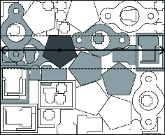
Figure 8: Detecting the overlapping pieces in the line search.

Let $N^{+}=\bigcup_{1\leq j\leq n,j\not=k}I_{kj}$ be the set of $t$ ($\in N$) inducing overlap with other pieces, and $N^{-}=N\setminus N^{+}$ be its complement. If $N^{-}\not=\emptyset$ holds, then the line search algorithm finds the minimum $t\in N^{-}$ (i.e., the left most feasible position); otherwise, it finds the position $t\in N^{+}$ that minimizes the overlap penalty function $\widetilde{F}_{k}(\bm{v}_{k}+t\bm{d},o_{k}^{\prime})$.

We now consider how to compute the overlap penalty function $f_{kj}(\bm{v}_{k}+t\bm{d},\bm{v}_{j},o_{k}^{\prime},o_{j})$ defined in (5) for a given $t\in N$, where $I_{kj}\not=\emptyset$ is assumed. Let $\bm{v}_{k}^{\prime}=\bm{v}_{k}+t\bm{d}$ be the position of the piece $P_{k}(o_{k}^{\prime})$ for a given $t\in N$. If $t\not\in I_{kj}$ holds, then $f_{kj}(\bm{v}_{k}^{\prime},\bm{v}_{j},o_{k}^{\prime},o_{j})=0$; otherwise, the overlap penalty $f_{kj}(\bm{v}_{k}^{\prime},\bm{v}_{j},o_{k}^{\prime},o_{j})$ is decomposed into the horizontal and vertical penetration depths. We denote the horizontal and vertical penetration depths for a given $t\in N$ by

$$\delta(P_{k}(o_{k}^{\prime})\oplus\bm{v}_{k}^{\prime},P_{j}(o_{j})\oplus\bm{v}_{j},\bm{d})=\min\{|s|\mid\bm{v}_{k}^{\prime}-\bm{v}_{j}+s\bm{d}\not\in\mathrm{NFP}(P_{j}(o_{j}),P_{k}(o_{k}^{\prime})\},$$ (13)

for $\bm{d}\in\{(1,0),(0,1)\}$, respectively. Figure 9 shows an example of computing the horizontal and vertical penetration depths in the line search from NFP of the double scanline representation.

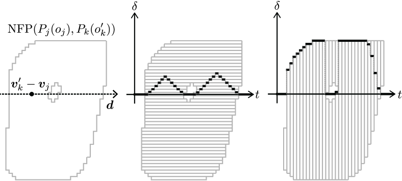
Figure 9: Computing the horizontal and vertical penetration depth in the line search.

Recall the horizontal and vertical scanline representations of $\mathrm{NFP}(P_{j}(o_{j}),P_{k}(o_{k}^{\prime}))$ in Figure 6. When the relative position $\bm{v}_{k}^{\prime}-\bm{v}_{j}$ of the piece $P_{k}(o_{k}^{\prime})$ is placed in a strip, the horizontal (resp., vertical) penetration depth then takes the minimum distance $|s|$ from $\bm{v}_{k}^{\prime}-\bm{v}_{j}$ to left and right (resp., bottom and top) side of the strip.

The line search algorithm is very time consuming when $|N^{+}|$ becomes larger according to high-resolution of the raster representation as long as it computes the overlap penalty $\widetilde{F}_{k}(\bm{v}_{k}+t\bm{d},o_{k}^{\prime})$ for all $t\in N^{+}$. As shown in Figure 9, the horizontal penetration depth forms a regular stepwise with steady changes, and it possibly takes the minimum value only at the left and right end of the strips on the horizontal line $\bm{v}_{k}+t\bm{d}$ ($t\in N$). On the other hand, the vertical penetration depth forms an irregular stepwise function that sometimes changes rapidly; however, it may occur only at the “corners” of $\mathrm{NFP}(P_{j}(o_{j}),P_{k}(o_{k}^{\prime}))$. We accordingly introduce a corner detection technique to restrict the search space of the line search only having rapid changes of the vertical penetration depth. We first detect the contour of $\mathrm{NFP}(P_{j}(o_{j}),P_{k}(o_{k}^{\prime}))$ and then apply a fast corner detection algorithm called FAST [Rosten & Drummond, 2006] to the contour as shown in Figure 10.

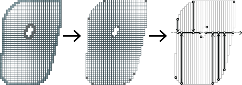
Figure 10: The corner detection algorithm for the NFP.

Let $\overline{\mathrm{NFP}}(P_{j}(o_{j}),P_{k}(o_{k}^{\prime}))$ be the set of detected corners in $\mathrm{NFP}(P_{j}(o_{j}),P_{k}(o_{k}^{\prime}))$ obtained by the FAST. We consider the set of positions $\bar{I}_{kj}$ ($\subseteq I_{kj}$) of the piece $P_{k}(o_{k}^{\prime})$ in terms of $t\in N$ that contains (i) the left and right end of the horizontal strips on the horizontal line $\bm{v}_{k}+t\bm{d}$ ($t\in N^{+}$), and (ii) the projection of $\overline{\mathrm{NFP}}(P_{j}(o_{j}),P_{k}(o_{k}^{\prime}))$ onto the horizontal line $\bm{v}_{k}+t\bm{d}$ ($t\in N^{+}$). Let $\overline{N}^{+}=\bigcup_{1\leq j\leq n,j\not=k}\bar{I}_{kj}$ ($\subseteq N^{+}$) be the reduced search space of the line search; i.e., the line search algorithm computes the weighted overlap penalty $\widetilde{F}_{k}(\bm{v}_{k}+t\bm{d},o_{k}^{\prime})$ only for $t\in\overline{N}^{+}$ (instead of $N^{+}$) when $N^{-}=\emptyset$ holds. In Figure 10 (right), the grey nodes show the detected corners in $\overline{\mathrm{NFP}}(P_{j}(o_{j}),P_{k}(o_{k}^{\prime}))$ by FAST, and the white nodes show the positions in $\bar{I}_{kj}$ to be evaluated by the line search algorithm.

4.3 Guided local search

It is often the case that CDH alone may not attain a sufficiently good solution. To improve its performance, we incorporate it into one of the representative metaheuristics called the guided local search (GLS) [Voudouris & Tsang, 1999]. The GLS repeats CDH while updating the penalty weights of the objective function adaptively to resume the search from the previous locally optimal solution. The GLS starts from an initial solution $(\bm{v},\bm{o})$ with some overlapping pieces, where the penalty weights $\alpha_{ij}$ are initialized to $1.0$. Whenever CDH stops at a locally optimal solution $(\bm{v},\bm{o})$, GLS updates the penalty weights $\alpha_{ij}$ by the following formula:

$$\alpha_{ij}\leftarrow\alpha_{ij}+\displaystyle\frac{f_{ij}(\bm{v}_{i},\bm{v}_{j},o_{i},o_{j})}{\displaystyle\max_{1\leq k<l\leq n}f_{kl}(\bm{v}_{k},\bm{v}_{l},o_{k},o_{l})},\quad 1\leq i<j\leq n.$$ (14)

By updating the penalty weights $\alpha_{ij}$ ($1\leq i<j\leq n$) repeatedly, the current solution $(\bm{v},\bm{o})$ becomes no longer locally optimal under the updated weighted overlap penalty function $\widetilde{F}$, and GLS resumes the search from the current solution. The GLS stops these operations if it fails to improve the best solution $(\bm{v}^{\ast},\bm{o}^{\ast})$ of the original penalty function $F$ after a specified number $k_{\max}$ of consecutive calls to CDH. The GLS is formally described in Algorithm 4.

Algorithm 4 GLS($L,\bm{v},\bm{o}$)

1:

2:$(\tilde{\bm{v}},\tilde{\bm{o}})\leftarrow(\bm{v},\bm{o})$, $(\bm{v}^{\ast},\bm{o}^{\ast})\leftarrow(\bm{v},\bm{o})$, $\alpha_{ij}\leftarrow 1.0$ ($1\leq i<j\leq n$), $k\leftarrow 0$

3:while $k<k_{\max}$ do

4:    $(\bm{v}^{\prime},\bm{o}^{\prime}),(\tilde{\bm{v}},\tilde{\bm{o}})\leftarrow\textnormal{CDH}(L,\tilde{\bm{v}},\tilde{\bm{o}})$ {See Algorithm 3}

5:    if $F(\bm{v}^{\prime},\bm{o}^{\prime})<F(\bm{v}^{\ast},\bm{o}^{\ast})$ then

6:         $(\bm{v}^{\ast},\bm{o}^{\ast})\leftarrow(\bm{v}^{\prime},\bm{o}^{\prime})$, $k\leftarrow 0$

7:         if $F(\bm{v}^{\ast},\bm{o}^{\ast})=0$ then

8:             Return $(\bm{v}^{\ast},\bm{o}^{\ast})$              

9:    Update the penalty weights $\alpha_{ij}$ ($1\leq i<j\leq n$) of $(\tilde{\bm{v}},\tilde{\bm{o}})$ by (14)

10:    $k\leftarrow k+1$

11:Return $(\bm{v}^{\ast},\bm{o}^{\ast})$

5 Construction algorithm for the initial layout

We generate an initial solution $(\bm{v},\bm{o})$ for ISP using the next-fit decreasing height (NFDH) algorithm. The NFDH is a variant of the level algorithms for the rectangle packing problem [Hu et al., 2018b] that places rectangle pieces from bottom to top in columns forming levels as shown in Figure 11. The first level is the left side of the container, and each subsequent level is along the vertical line coinciding with the right of the longest piece placed in the previous level. The NFDH first sorts the pieces $P_{i}$ ($1\leq i\leq n$) in the descending order of the lengths $l_{i}$ of their bounding-boxes, where they are not rotated (i.e., $l_{i}=l_{i}(0)$). Let the container length $L$ be sufficiently long, e.g., $L>\sum_{1\leq i\leq n}l_{i}$. The NFDH places all pieces $P_{i}$ ($1\leq i\leq n$) one by one into the container $C$ according to the above order. If possible, each piece $P_{i}$ (more precisely, its bounding-box) is placed at the bottom-most feasible position in the current level; otherwise, a new level is created to place the piece $P_{i}$. We then apply a compaction algorithm (called Compact) based on the bottom-left strategy that makes successive sliding moves to the left and the bottom alternately as long as possible. The compaction algorithm can be implemented based on the neighborhood search (Algorithm 2) by replacing the condition $\widetilde{F}_{k}(\bm{v}_{k}^{\prime}+t\bm{d},o_{k}^{\prime})<\widetilde{F}_{k}(\bm{v}_{k}^{\prime},o_{k}^{\prime})$ with $t<0$ (i.e., the piece $P_{k}$ slides to the left or the bottom without overlap). They are formally described in Algorithm 5.

Algorithm 5 Construct

1:

2:$L\leftarrow 0$, $\bar{l}\leftarrow 0$, $\bar{w}\leftarrow 0$

3:for $P_{i}$ ($1\leq i\leq n$) in the descending order of $l_{i}$ do

4:    if $\bar{w}+w_{i}>W$ then

5:         $L\leftarrow L+\bar{l}$, $\bar{w}\leftarrow 0$, $\bar{l}\leftarrow 0$     

6:    $\bm{v}_{i}\leftarrow(L+\lfloor\frac{l_{i}}{2}\rfloor,\bar{w}+\lfloor\frac{w_{i}}{2}\rfloor)$, $\bar{w}\leftarrow\bar{w}+w_{i}$, $\bar{l}\leftarrow\max\{\bar{l},l_{i}\}$

7:for $P_{i}$ ($1\leq i\leq n$) in the descending order of $l_{i}$ do

8:    $(\bm{v},\bm{o})\leftarrow\textnormal{{\sc Compact}}(L,\bm{v},\bm{o},P_{i},0)$

9:$L\leftarrow\displaystyle\max_{1\leq i\leq n}\left(x_{i}+\lfloor\textstyle\frac{l_{i}}{2}\rfloor\right)$

10:Return $L$, $(\bm{v},\bm{o})$

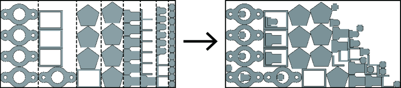
Figure 11: Constructing an initial solution for ISP.

6 Computational results

The guided coordinate descent heuristics (GCDH) proposed in this paper were implemented with the C programming language and run on a single thread under a Mac PC with a 3.2 GHz Intel Core i7 processor and 64 GB memory. We set the input parameters $r_{\mathrm{dec}}=0.02$, $r_{\mathrm{inc}}=0.005$ for GCDH (Algorithm 1) and $k_{\max}=200$ for GLS (Algorithm 4) according to Umetani et al. [2009]. The performance of GCDH was tested on two sets of instances for ISP represented in the vector model. The first set includes 15 instances of the standard vector model without circular arcs nor holes (i.e., the simple polygon packing problem), which are available online at the web site of the working group on cutting and packing [ESICUP, 2003]. The second set includes 10 instances of an extended vector model, in which several instances incorporate circular arcs and holes into polygons [Burke et al., 2010]. Table 1 summarizes the data of the instances. The second column “#shapes” shows the number of different shapes, the third column “#pieces” shows the total number of pieces, the fourth column “avg.#lines” shows the average number of the line segments in an irregular shape, the fifth column “avg.#arcs” shows the average number of the circular arcs in an irregular shape, the sixth column “avg.#holes” shows the average number of holes in an irregular shape, and the seventh column “degrees” shows the permitted orientations, where we note that the permitted orientations are common to all pieces in each instance.

Table 1: The test instances of ISP

instance	#shapes	#pieces	avg.#lines	avg.#arcs	avg.#holes	degrees
Albano	8	24	6.83	0.00	0.00	0, 180 absolute
Dagli	10	30	7.30	0.00	0.00	0, 180 absolute
Dighe1	16	16	3.88	0.00	0.00	0 absolute
Dighe2	10	10	4.70	0.00	0.00	0 absolute
Fu	11	12	3.58	0.00	0.00	90 incremental
Jakobs1	25	25	6.00	0.00	0.00	90 incremental
Jakobs2	25	25	5.36	0.00	0.00	90 incremental
Mao	9	20	8.70	0.00	0.00	90 incremental
Marques	8	24	7.08	0.00	0.00	90 incremental
Shapes0	4	43	6.29	0.00	0.00	0 absolute
Shapes1	4	43	6.29	0.00	0.00	0, 180 absolute
Shirts	8	99	6.05	0.00	0.00	0, 180 absolute
Swim	10	48	20.0	0.00	0.00	0, 180 absolute
Trousers	17	64	5.94	0.00	0.00	0, 180 absolute
Profiles1	8	32	4.63	0.63	0.00	90 incremental
Profiles2	7	50	7.54	1.50	0.38	90 incremental
Profiles3	6	46	7.93	0.65	0.00	45 incremental
Profiles4	7	54	3.83	0.41	0.00	90 incremental
Profiles5	5	50	7.19	0.00	0.13	15 incremental
Profiles6	9	69	4.60	1.40	0.00	90 incremental
Profiles7	9	9	4.67	0.00	0.00	90 incremental
Profiles8	9	18	4.67	0.00	0.00	90 incremental
Profiles9	16	57	26.61	0.00	0.16	90 incremental
Profiles10	13	91	8.23	0.00	0.00	0 absolute

We converted these instances into the raster model with five different resolutions; i.e., we set the width $W$ of the container $C$ to 128, 256, 512, 1024 and 2048 pixels. Tables 2 and 3 show the instance size of the raster model for the instances (i.e., the number of pixels for representing all the irregular shapes) and the memory usage when running GCDH, respectively.

Table 2: The instance size of the raster model (in pixels)

instance	$W=128\mathrm{px}$	$W=256\mathrm{px}$	$W=512\mathrm{px}$	$W=1024\mathrm{px}$	$W=2048\mathrm{px}$
Albano	$3.02\times 10^{4}$	$1.19\times 10^{5}$	$4.70\times 10^{5}$	$1.87\times 10^{6}$	$7.47\times 10^{6}$
Dagli	$1.46\times 10^{4}$	$5.69\times 10^{4}$	$2.25\times 10^{5}$	$8.94\times 10^{5}$	$3.56\times 10^{6}$
Dighe1	$1.74\times 10^{4}$	$6.76\times 10^{4}$	$2.66\times 10^{5}$	$1.06\times 10^{6}$	$4.21\times 10^{6}$
Dighe2	$1.70\times 10^{4}$	$6.71\times 10^{4}$	$2.64\times 10^{5}$	$1.05\times 10^{6}$	$4.20\times 10^{6}$
Fu	$1.25\times 10^{4}$	$4.94\times 10^{4}$	$1.98\times 10^{5}$	$7.88\times 10^{5}$	$3.15\times 10^{6}$
Jakobs1	$4.20\times 10^{3}$	$1.64\times 10^{4}$	$6.53\times 10^{4}$	$2.59\times 10^{5}$	$1.03\times 10^{6}$
Jakobs2	$4.89\times 10^{3}$	$1.89\times 10^{4}$	$7.41\times 10^{4}$	$2.92\times 10^{5}$	$1.16\times 10^{6}$
Mao	$1.00\times 10^{4}$	$3.94\times 10^{4}$	$1.55\times 10^{5}$	$6.12\times 10^{5}$	$2.44\times 10^{6}$
Marques	$1.15\times 10^{4}$	$4.49\times 10^{4}$	$1.77\times 10^{5}$	$7.02\times 10^{5}$	$2.80\times 10^{6}$
Shapes0	$1.74\times 10^{4}$	$6.80\times 10^{4}$	$2.68\times 10^{5}$	$1.06\times 10^{6}$	$4.20\times 10^{6}$
Shapes1	$1.74\times 10^{4}$	$6.80\times 10^{4}$	$2.68\times 10^{5}$	$1.06\times 10^{6}$	$4.20\times 10^{6}$
Shirts	$2.32\times 10^{4}$	$9.12\times 10^{4}$	$3.61\times 10^{5}$	$1.43\times 10^{6}$	$5.68\times 10^{6}$
Swim	$1.45\times 10^{4}$	$5.43\times 10^{4}$	$2.09\times 10^{5}$	$8.24\times 10^{5}$	$3.26\times 10^{6}$
Trousers	$4.68\times 10^{4}$	$1.83\times 10^{5}$	$7.30\times 10^{5}$	$2.90\times 10^{6}$	$1.16\times 10^{7}$
Profiles1	$1.01\times 10^{4}$	$3.90\times 10^{4}$	$1.52\times 10^{5}$	$6.03\times 10^{5}$	$2.40\times 10^{6}$
Profiles2	$1.71\times 10^{4}$	$6.44\times 10^{4}$	$2.54\times 10^{5}$	$1.01\times 10^{6}$	$4.00\times 10^{6}$
Profiles3	$3.96\times 10^{4}$	$1.55\times 10^{5}$	$6.04\times 10^{5}$	$2.39\times 10^{6}$	$9.52\times 10^{6}$
Profiles4	$7.22\times 10^{4}$	$2.84\times 10^{5}$	$1.12\times 10^{6}$	$4.46\times 10^{6}$	$1.78\times 10^{7}$
Profiles5	$1.17\times 10^{4}$	$4.51\times 10^{4}$	$1.76\times 10^{5}$	$6.91\times 10^{5}$	$2.74\times 10^{6}$
Profiles6	$8.75\times 10^{3}$	$3.39\times 10^{4}$	$1.29\times 10^{5}$	$5.04\times 10^{5}$	$1.99\times 10^{6}$
Profiles7	$3.40\times 10^{4}$	$1.33\times 10^{5}$	$5.29\times 10^{5}$	$2.11\times 10^{6}$	$8.41\times 10^{6}$
Profiles8	$1.76\times 10^{4}$	$6.79\times 10^{4}$	$2.66\times 10^{5}$	$1.06\times 10^{6}$	$4.21\times 10^{6}$
Profiles9	$9.68\times 10^{3}$	$3.42\times 10^{4}$	$1.29\times 10^{5}$	$4.97\times 10^{5}$	$1.95\times 10^{6}$
Profiles10	$4.42\times 10^{4}$	$1.69\times 10^{5}$	$6.59\times 10^{5}$	$2.62\times 10^{6}$	$1.04\times 10^{7}$
avg.(all)	$2.11\times 10^{4}$	$8.21\times 10^{4}$	$3.23\times 10^{5}$	$1.28\times 10^{6}$	$5.10\times 10^{6}$

Table 3: The memory usage when running GCDH (in MB)

instance	$W=128\mathrm{px}$	$W=256\mathrm{px}$	$W=512\mathrm{px}$	$W=1024\mathrm{px}$	$W=2048\mathrm{px}$
Albano	31	136	409	1656	2216
Dagli	10	34	165	561	2061
Dighe1	25	111	420	1586	2789
Dighe2	28	99	326	1689	2139
Fu	30	77	267	848	2480
Jakobs1	23	71	170	530	1624
Jakobs2	25	72	185	503	1743
Mao	22	60	383	1219	2704
Marques	18	67	267	979	2650
Shapes0	4	9	63	397	1170
Shapes1	6	14	62	483	1689
Shirts	7	20	67	479	1316
Swim	6	33	222	700	1920
Trousers	16	65	316	1029	2064
Profiles1	12	52	174	501	2231
Profiles2	14	68	197	541	2548
Profiles3	90	292	1122	2130	3226
Profiles4	27	100	450	1725	2964
Profiles5	65	173	407	1007	2642
Profiles6	5	17	49	246	985
Profiles7	106	436	1539	2554	4501
Profiles8	26	124	456	1495	2776
Profiles9	31	114	381	1210	3078
Profiles10	19	36	205	805	2401
avg.(all)	26.9	95.0	345.9	1036.4	2329.9

Figure 12 shows the best solutions for a test instance in different resolutions. We note that the rasterized shapes (especially in the low-resolution, e.g., $W=128$px) are rather different from the original shapes in the vector model, which often leads different optimal solutions. For example, diagonal straight lines in the vector model are often converted into jagged ones in the raster model of the low-resolution, which prevents the pieces from sticking together precisely. We also encounter other cases that complicated shapes in the vector model are converted into simple ones in the raster model of the low-resolution, which enables GCDH to perform efficiently and attain better solutions. We accordingly use the instances of the middle-resolution $W=512$px in the comparison with the other algorithms for the vector model.

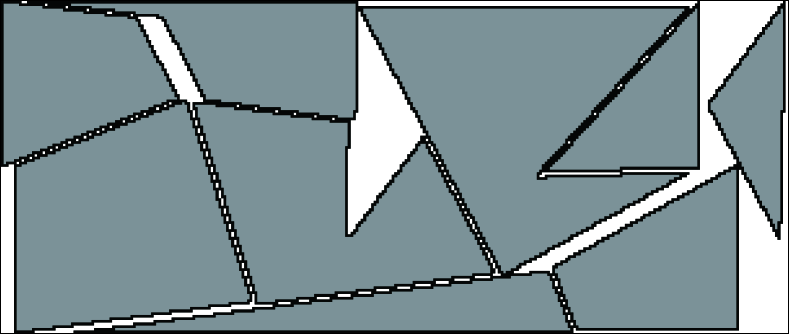
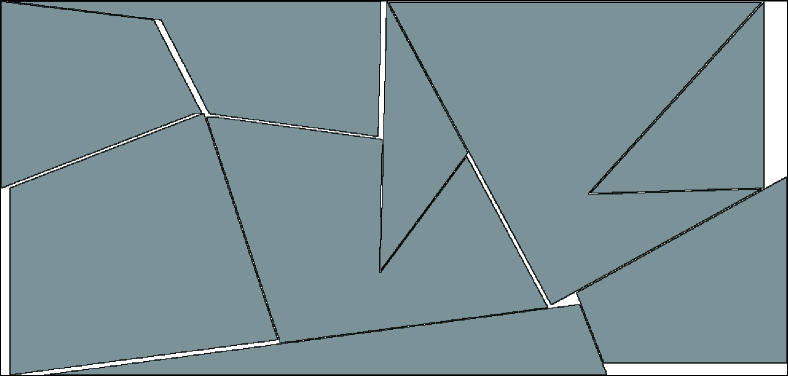
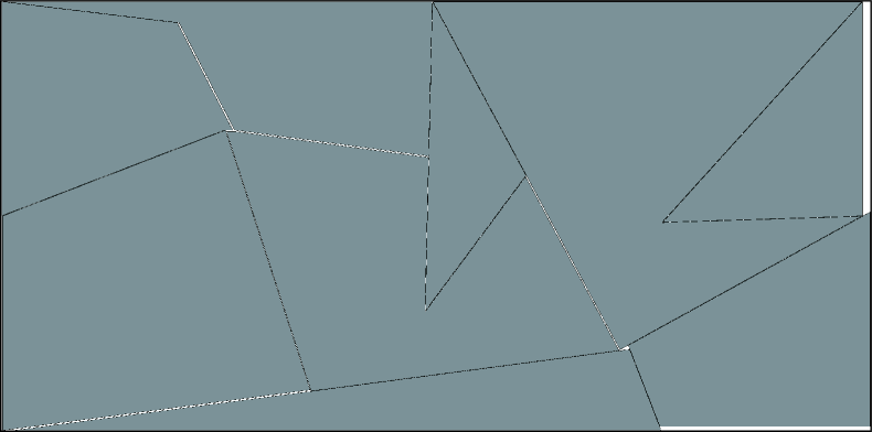
Figure 12: The best solutions for a test instance in different resolutions (Left: $W=128$px, Center: $W=512$px, Right: $W=2048$px)

Tables 4 and 5 show the computation time of the preprocessing in seconds for generating NFPs for all pairs of different shapes and detecting corners for all generated NFPs.

Table 4: The computation time to generate NFPs (in seconds)

instance	$W=128\mathrm{px}$	$W=256\mathrm{px}$	$W=512\mathrm{px}$	$W=1024\mathrm{px}$	$W=2048\mathrm{px}$
Albano	0.03	0.12	0.48	1.99	8.15
Dagli	0.01	0.05	0.22	0.85	3.51
Dighe1	0.05	0.19	0.77	3.21	13.16
Dighe2	0.03	0.11	0.44	1.81	7.38
Fu	0.07	0.25	1.01	4.03	16.44
Jakobs1	0.04	0.15	0.58	2.27	9.00
Jakobs2	0.06	0.22	0.88	3.47	13.94
Mao	0.03	0.11	0.42	1.74	7.04
Marques	0.02	0.08	0.32	1.32	5.33
Shapes0	$<$0.01	0.01	0.03	0.12	0.48
Shapes1	$<$0.01	0.02	0.06	0.24	0.98
Shirts	0.01	0.02	0.09	0.37	1.49
Swim	0.02	0.06	0.25	1.01	4.10
Trousers	0.06	0.22	0.90	3.68	14.81
Profiles1	0.01	0.06	0.22	0.85	3.44
Profiles2	0.03	0.10	0.43	1.73	7.09
Profiles3	0.19	0.78	3.19	13.06	52.76
Profiles4	0.04	0.17	0.67	2.75	11.13
Profiles5	0.16	0.62	2.47	9.95	39.99
Profiles6	0.01	0.06	0.23	0.93	3.92
Profiles7	0.29	1.16	4.75	19.38	77.34
Profiles8	0.07	0.28	1.15	4.77	19.22
Profiles9	0.10	0.42	1.77	7.32	30.02
Profiles10	0.02	0.07	0.29	1.19	4.78
avg.(all)	0.06	0.22	0.90	3.67	14.81

Table 5: The computation time for the corner detection (in seconds)

instance	$W=128\mathrm{px}$	$W=256\mathrm{px}$	$W=512\mathrm{px}$	$W=1024\mathrm{px}$	$W=2048\mathrm{px}$
Albano	0.06	0.20	0.98	4.12	10.81
Dagli	0.03	0.08	0.29	1.65	5.83
Dighe1	0.07	0.26	1.48	6.81	17.31
Dighe2	0.04	0.14	0.79	3.71	9.98
Fu	0.14	0.43	1.82	8.98	29.19
Jakobs1	0.19	0.44	1.31	5.27	28.02
Jakobs2	0.21	0.53	1.56	6.67	35.49
Mao	0.09	0.26	1.20	6.05	16.85
Marques	0.06	0.17	0.72	3.73	12.32
Shapes0	$<$0.01	0.02	0.07	0.39	1.21
Shapes1	0.01	0.03	0.12	0.73	2.20
Shirts	0.02	0.04	0.15	0.82	3.27
Swim	0.03	0.12	0.57	2.77	9.79
Trousers	0.08	0.24	1.01	4.95	14.13
Profiles1	0.05	0.13	0.43	1.77	7.34
Profiles2	0.05	0.14	0.49	2.30	9.03
Profiles3	0.38	1.60	8.95	30.99	77.15
Profiles4	0.08	0.32	1.59	5.72	16.52
Profiles5	0.52	1.42	4.59	18.37	73.86
Profiles6	0.03	0.08	0.24	1.03	5.59
Profiles7	0.45	2.16	10.60	27.01	118.71
Profiles8	0.14	0.43	2.15	10.06	26.75
Profiles9	0.18	0.55	2.25	12.22	43.48
Profiles10	0.04	0.12	0.51	2.69	8.59
avg.(all)	0.12	0.41	1.83	7.03	24.31

Figures 13 and 14 show the evolution of density (%) when GCDH running 10 times on Swim instance with the time limit of 18000 seconds. The GCDH starts from an initial solution of the density 42.47% obtained by the construction algorithm (Algorithm 5), and then rapidly improves it within several seconds to attain the density over 70%. We observed that GCDH performs similarly for other instances.

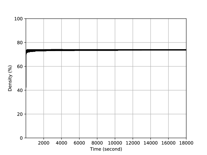
Figure 13: The evolutions of density when GCDH running 10 times on Swim instance (normal plot)

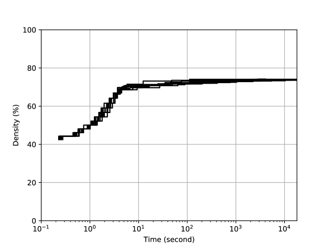
Figure 14: The evolutions of density when GCDH running 10 times on Swim instance (linear-log plot)

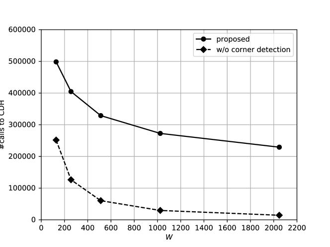
Figure 15: The number of calls to CDH when running GCDH (normal plot)

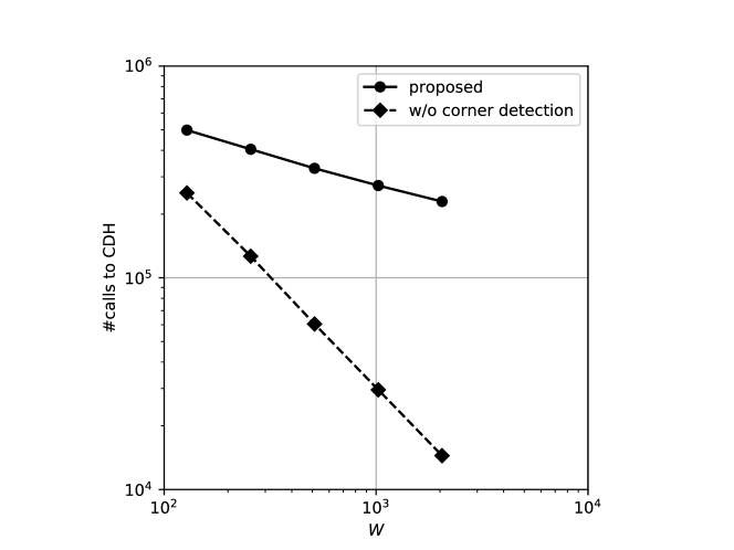
Figure 16: The number of calls to CDH when running GCDH (log-log plot)

We first evaluated the effect of the corner detection technique on GCDH. We tested GCDH 10 times for each instance with the time limit of 1200 seconds for each run, which is the same for all resolutions and does not include the computation time of the preprocessing for generating NFPs and detecting their corners (Tables 4 and 5). Tables 6 and 7 show the number of calls to CDH (Algorithm 3) with and without the corner detection, respectively. Table 8 shows the improvement in the computational efficiency of GCDH via the corner detection with respect to the number of calls to CDH, where that of GCDH without it is set to one. The GCDH with the corner detection was 14.08 times faster on average than GCDH without it for the instances of high-resolution ($W=2048$px). Figures 15 and 16 also show the average number of calls to CDH for all instances. The computational efficiency has been much improved by the corner detection technique; i.e., the numbers of calls to CDH decrease in proportion to the cube root of the value of $W$ roughly, while those decrease in proportion of that of $W$ without the corner detection.

Table 6: The number of calls to CDH when running GCDH with the corner detection

instance	$W=128\mathrm{px}$	$W=256\mathrm{px}$	$W=512\mathrm{px}$	$W=1024\mathrm{px}$	$W=2048\mathrm{px}$
Albano	$6.95\times 10^{5}$	$5.33\times 10^{5}$	$4.55\times 10^{5}$	$4.00\times 10^{5}$	$3.65\times 10^{5}$
Dagli	$4.55\times 10^{5}$	$3.44\times 10^{5}$	$2.75\times 10^{5}$	$2.45\times 10^{5}$	$2.33\times 10^{5}$
Dighe1	$1.17\times 10^{6}$	$8.07\times 10^{5}$	$6.11\times 10^{5}$	$4.88\times 10^{5}$	$3.93\times 10^{5}$
Dighe2	$2.92\times 10^{6}$	$2.56\times 10^{6}$	$2.05\times 10^{6}$	$1.55\times 10^{6}$	$1.24\times 10^{6}$
Fu	$1.40\times 10^{6}$	$1.24\times 10^{6}$	$1.05\times 10^{6}$	$9.42\times 10^{5}$	$7.89\times 10^{5}$
Jakobs1	$3.25\times 10^{5}$	$2.72\times 10^{5}$	$2.23\times 10^{5}$	$2.08\times 10^{5}$	$1.62\times 10^{5}$
Jakobs2	$2.72\times 10^{5}$	$2.07\times 10^{5}$	$1.80\times 10^{5}$	$1.50\times 10^{5}$	$1.17\times 10^{5}$
Mao	$4.97\times 10^{5}$	$4.53\times 10^{5}$	$3.58\times 10^{5}$	$2.87\times 10^{5}$	$2.54\times 10^{5}$
Marques	$4.13\times 10^{5}$	$3.78\times 10^{5}$	$2.97\times 10^{5}$	$2.39\times 10^{5}$	$2.16\times 10^{5}$
Shapes0	$4.40\times 10^{5}$	$3.44\times 10^{5}$	$3.13\times 10^{5}$	$2.98\times 10^{5}$	$2.85\times 10^{5}$
Shapes1	$1.95\times 10^{5}$	$1.60\times 10^{5}$	$1.32\times 10^{5}$	$1.25\times 10^{5}$	$1.07\times 10^{5}$
Shirts	$1.11\times 10^{5}$	$7.98\times 10^{4}$	$6.12\times 10^{4}$	$5.08\times 10^{4}$	$4.40\times 10^{4}$
Swim	$1.98\times 10^{5}$	$1.22\times 10^{5}$	$8.72\times 10^{4}$	$7.02\times 10^{4}$	$5.80\times 10^{4}$
Trousers	$1.98\times 10^{5}$	$1.51\times 10^{5}$	$1.38\times 10^{5}$	$1.14\times 10^{5}$	$9.36\times 10^{4}$
Profiles1	$2.44\times 10^{5}$	$1.77\times 10^{5}$	$1.54\times 10^{5}$	$1.43\times 10^{5}$	$1.17\times 10^{5}$
Profiles2	$1.06\times 10^{5}$	$7.49\times 10^{4}$	$6.67\times 10^{4}$	$5.82\times 10^{4}$	$4.78\times 10^{4}$
Profiles3	$2.87\times 10^{4}$	$2.07\times 10^{4}$	$1.71\times 10^{4}$	$1.53\times 10^{4}$	$1.18\times 10^{4}$
Profiles4	$5.97\times 10^{4}$	$4.67\times 10^{4}$	$4.14\times 10^{4}$	$3.47\times 10^{4}$	$3.46\times 10^{4}$
Profiles5	$2.36\times 10^{4}$	$1.40\times 10^{4}$	$9.82\times 10^{3}$	$8.61\times 10^{3}$	$6.66\times 10^{3}$
Profiles6	$8.64\times 10^{4}$	$6.20\times 10^{4}$	$4.21\times 10^{4}$	$3.32\times 10^{4}$	$2.53\times 10^{4}$
Profiles7	$1.50\times 10^{6}$	$1.19\times 10^{6}$	$9.60\times 10^{5}$	$7.74\times 10^{5}$	$6.66\times 10^{5}$
Profiles8	$4.44\times 10^{5}$	$3.60\times 10^{5}$	$2.82\times 10^{5}$	$2.43\times 10^{5}$	$1.90\times 10^{5}$
Profiles9	$1.02\times 10^{5}$	$6.60\times 10^{4}$	$4.59\times 10^{4}$	$3.31\times 10^{4}$	$2.78\times 10^{4}$
Profiles10	$6.74\times 10^{4}$	$5.01\times 10^{4}$	$3.99\times 10^{4}$	$3.25\times 10^{4}$	$2.52\times 10^{4}$
avg.(all)	$4.98\times 10^{5}$	$4.05\times 10^{5}$	$3.29\times 10^{5}$	$2.73\times 10^{5}$	$2.29\times 10^{5}$

Table 7: The number of calls to CDH when running GCDH without the corner detection

instance	$W=128\mathrm{px}$	$W=256\mathrm{px}$	$W=512\mathrm{px}$	$W=1024\mathrm{px}$	$W=2048\mathrm{px}$
Albano	$2.84\times 10^{5}$	$1.38\times 10^{5}$	$6.90\times 10^{4}$	$3.41\times 10^{4}$	$1.64\times 10^{4}$
Dagli	$2.61\times 10^{5}$	$1.26\times 10^{5}$	$6.07\times 10^{4}$	$3.02\times 10^{4}$	$1.45\times 10^{4}$
Dighe1	$5.84\times 10^{5}$	$2.71\times 10^{5}$	$1.28\times 10^{5}$	$6.58\times 10^{4}$	$3.30\times 10^{4}$
Dighe2	$1.30\times 10^{6}$	$6.92\times 10^{5}$	$3.35\times 10^{5}$	$1.53\times 10^{5}$	$7.15\times 10^{4}$
Fu	$6.15\times 10^{6}$	$3.17\times 10^{5}$	$1.49\times 10^{5}$	$7.49\times 10^{4}$	$3.66\times 10^{4}$
Jakobs1	$2.37\times 10^{5}$	$1.22\times 10^{5}$	$6.20\times 10^{4}$	$3.27\times 10^{4}$	$1.51\times 10^{4}$
Jakobs2	$2.20\times 10^{5}$	$9.68\times 10^{4}$	$4.89\times 10^{4}$	$2.59\times 10^{4}$	$1.30\times 10^{4}$
Mao	$3.73\times 10^{5}$	$2.09\times 10^{5}$	$9.88\times 10^{4}$	$4.45\times 10^{4}$	$2.28\times 10^{4}$
Marques	$2.56\times 10^{5}$	$1.44\times 10^{5}$	$6.90\times 10^{4}$	$3.37\times 10^{4}$	$1.64\times 10^{4}$
Shapes0	$2.85\times 10^{5}$	$1.39\times 10^{5}$	$6.87\times 10^{4}$	$3.72\times 10^{4}$	$2.01\times 10^{4}$
Shapes1	$1.36\times 10^{5}$	$7.16\times 10^{4}$	$3.27\times 10^{4}$	$1.80\times 10^{4}$	$8.76\times 10^{3}$
Shirts	$7.91\times 10^{4}$	$3.70\times 10^{4}$	$1.68\times 10^{4}$	$7.89\times 10^{3}$	$3.78\times 10^{3}$
Swim	$1.55\times 10^{5}$	$7.06\times 10^{4}$	$3.08\times 10^{4}$	$1.44\times 10^{4}$	$7.12\times 10^{3}$
Trousers	$8.84\times 10^{4}$	$3.92\times 10^{4}$	$1.90\times 10^{4}$	$9.26\times 10^{3}$	$4.54\times 10^{3}$
Profiles1	$1.78\times 10^{5}$	$9.05\times 10^{4}$	$4.34\times 10^{4}$	$2.15\times 10^{4}$	$1.08\times 10^{4}$
Profiles2	$7.80\times 10^{4}$	$3.75\times 10^{4}$	$1.85\times 10^{4}$	$9.08\times 10^{3}$	$4.65\times 10^{3}$
Profiles3	$1.80\times 10^{4}$	$8.39\times 10^{3}$	$4.18\times 10^{3}$	$2.02\times 10^{3}$	$1.11\times 10^{3}$
Profiles4	$2.01\times 10^{4}$	$1.01\times 10^{4}$	$4.95\times 10^{3}$	$2.47\times 10^{3}$	$1.32\times 10^{3}$
Profiles5	$1.94\times 10^{4}$	$8.24\times 10^{3}$	$3.67\times 10^{3}$	$1.69\times 10^{3}$	$8.09\times 10^{2}$
Profiles6	$6.99\times 10^{4}$	$3.49\times 10^{4}$	$1.68\times 10^{4}$	$8.29\times 10^{3}$	$3.90\times 10^{3}$
Profiles7	$4.35\times 10^{7}$	$2.05\times 10^{5}$	$9.31\times 10^{4}$	$4.55\times 10^{4}$	$2.24\times 10^{4}$
Profiles8	$2.27\times 10^{5}$	$1.09\times 10^{5}$	$5.29\times 10^{4}$	$2.44\times 10^{4}$	$1.21\times 10^{4}$
Profiles9	$8.66\times 10^{4}$	$4.01\times 10^{4}$	$1.87\times 10^{4}$	$9.02\times 10^{3}$	$4.54\times 10^{3}$
Profiles10	$3.73\times 10^{4}$	$1.65\times 10^{4}$	$7.59\times 10^{3}$	$3.75\times 10^{3}$	$1.79\times 10^{3}$
avg.(all)	$2.52\times 10^{5}$	$1.26\times 10^{5}$	$6.05\times 10^{4}$	$2.96\times 10^{4}$	$1.45\times 10^{4}$

Table 8: The improvement in the computational efficiency of GCDH via the corner detection

instance	$W=128\mathrm{px}$	$W=256\mathrm{px}$	$W=512\mathrm{px}$	$W=1024\mathrm{px}$	$W=2048\mathrm{px}$
Albano	2.45	3.85	6.60	11.74	21.72
Dagli	1.74	2.72	4.53	8.12	16.07
Dighe1	2.01	2.98	4.76	7.42	11.89
Dighe2	2.25	3.70	6.13	10.11	17.38
Fu	2.27	3.90	7.08	12.58	21.52
Jakobs1	1.37	2.24	3.59	6.38	10.77
Jakobs2	1.24	2.14	3.68	5.80	9.01
Mao	1.33	2.17	3.62	6.44	11.16
Marques	1.61	2.63	4.30	7.09	13.20
Shapes0	1.55	2.47	4.56	8.02	14.23
Shapes1	1.44	2.23	4.05	6.94	12.22
Shirts	1.40	2.16	3.63	6.44	11.64
Swim	1.28	1.73	2.83	4.87	8.14
Trousers	2.24	3.86	7.23	12.34	20.62
Profiles1	1.37	1.96	3.54	6.66	10.83
Profiles2	1.36	2.00	3.61	6.40	10.26
Profiles3	1.59	2.46	4.09	7.58	10.61
Profiles4	2.97	4.62	8.35	14.06	26.16
Profiles5	1.21	1.70	2.68	5.09	8.23
Profiles6	1.24	1.78	2.50	4.00	6.47
Profiles7	3.46	5.80	10.31	17.01	29.71
Profiles8	1.95	3.30	5.33	9.96	15.74
Profiles9	1.18	1.64	2.45	3.67	6.12
Profiles10	1.81	3.03	5.26	8.68	14.12
avg.(all)	1.76	2.79	4.78	8.22	14.08

Tables 9 and 10 show the computational results obtained by GCDH with and without the corner detection respectively, which are evaluated in the best and average density (%). Table 11 shows the improvement in the average density (%) of GCDH via the corner detection. The improvement in the computational efficiency also brought that in the quality of the obtained solutions; e.g., GCDH with the corner detection attained 2.02 point better than GCDH without it in the average density (%) for the instances of high-resolution ($W=2048$px).

Table 9: The density (%) of solutions obtained by GCDH with the corner detection

instance	$W=128\mathrm{px}$			$W=256\mathrm{px}$			$W=512\mathrm{px}$			$W=1024\mathrm{px}$			$W=2048\mathrm{px}$
	best	avg.		best	avg.		best	avg.		best	avg.		best	avg.
Albano	89.01	88.74		88.20	87.75		88.20	87.47		87.68	87.09		87.08	86.80
Dagli	87.96	87.23		86.84	86.44		86.32	85.70		86.36	85.71		85.92	85.19
Dighe1	92.60	91.07		96.07	95.82		97.60	97.55		98.90	98.80		99.33	99.27
Dighe2	93.01	93.01		95.01	94.77		97.28	97.17		98.79	98.74		99.28	99.20
Fu	92.31	91.11		90.99	90.31		90.75	89.62		91.90	90.16		89.87	89.02
Jakobs1	88.58	84.94		84.32	84.32		88.01	86.54		88.48	86.71		87.98	86.68
Jakobs2	81.33	81.33		81.91	78.77		79.51	78.86		79.47	78.44		80.66	78.68
Mao	87.17	86.80		85.12	84.84		84.84	83.62		84.03	83.45		84.10	83.28
Marques	91.39	91.39		89.92	89.74		90.43	89.33		89.36	88.73		88.75	88.37
Shapes0	68.49	67.51		66.74	66.31		66.13	65.33		65.14	64.56		64.81	64.31
Shapes1	75.30	74.24		73.38	72.62		72.35	71.86		71.88	71.23		71.46	71.09
Shirts	86.72	86.39		85.82	85.06		84.33	84.14		84.43	83.68		84.24	83.50
Swim	78.87	77.27		74.74	73.99		74.08	72.91		73.60	72.52		72.99	72.21
Trousers	89.19	88.43		88.41	87.40		88.29	87.09		88.02	86.76		88.01	86.99
Profiles1	84.75	84.65		86.03	84.79		86.93	85.08		87.07	84.17		85.73	84.09
Profiles2	79.43	79.15		77.66	76.97		77.28	76.36		76.39	76.02		76.57	75.53
Profiles3	76.32	75.10		75.52	73.38		73.87	72.91		73.51	72.37		72.67	72.02
Profiles4	86.04	85.21		85.92	85.19		85.63	84.71		85.31	84.43		84.64	84.09
Profiles5	83.88	83.18		82.15	81.73		82.47	81.42		82.10	80.92		82.44	81.45
Profiles6	81.40	81.03		81.14	80.45		79.03	78.71		77.50	76.85		77.94	76.92
Profiles7	87.25	87.25		92.60	92.40		95.80	95.65		98.27	98.18		98.92	98.83
Profiles8	87.34	85.29		86.40	84.51		87.61	85.08		86.65	85.36		88.50	86.07
Profiles9	66.95	66.07		61.08	60.18		57.86	57.39		56.64	55.65		55.92	54.91
Profiles10	70.90	70.38		68.69	68.43		68.20	67.47		67.91	66.98		67.23	66.60
avg.(1st)	85.85	84.96		84.81	84.15		84.87	84.08		84.86	84.06		84.60	83.90
avg.(2nd)	80.42	79.73		79.74	78.84		79.38	78.42		79.22	78.09		79.06	78.05
avg.(all)	83.59	82.78		82.70	81.94		82.58	81.72		82.51	81.57		82.29	81.46

Table 10: The density (%) of solutions obtained by GCDH without the corner detection

instance	$W=128\mathrm{px}$			$W=256\mathrm{px}$			$W=512\mathrm{px}$			$W=1024\mathrm{px}$			$W=2048\mathrm{px}$
	best	avg.		best	avg.		best	avg.		best	avg.		best	avg.
Albano	89.01	88.68		88.54	87.80		87.61	86.79		87.89	86.38		86.54	85.71
Dagli	87.96	87.09		86.84	86.07		86.66	85.34		84.76	84.18		86.22	84.33
Dighe1	91.98	87.77		96.07	93.60		97.42	94.05		92.03	88.65		95.95	86.35
Dighe2	93.01	93.01		95.01	94.84		97.28	97.16		98.79	98.74		99.28	99.21
Fu	90.60	90.27		90.14	89.56		89.28	88.44		91.25	88.67		89.14	87.42
Jakobs1	84.03	84.03		89.00	85.26		86.82	84.42		85.20	83.36		85.15	82.94
Jakobs2	81.33	80.67		78.42	78.42		79.94	78.65		78.59	77.38		77.90	76.47
Mao	87.17	86.06		85.59	84.75		85.08	83.42		83.91	82.98		83.10	82.21
Marques	91.39	91.30		91.33	89.70		89.49	88.85		88.55	88.05		88.40	87.55
Shapes0	68.15	67.55		66.91	66.03		66.30	64.88		64.90	63.85		64.06	63.18
Shapes1	74.89	73.88		72.78	72.03		72.05	71.03		71.33	70.11		70.65	69.90
Shirts	87.55	86.67		85.61	85.04		84.53	83.84		83.90	83.19		83.96	83.00
Swim	77.26	76.79		74.22	73.81		73.28	72.38		72.21	71.49		71.74	70.88
Trousers	89.19	88.16		88.30	87.00		87.32	86.44		86.54	85.57		87.15	85.66
Profiles1	84.75	84.75		84.59	83.90		84.70	83.73		85.18	82.63		84.32	82.55
Profiles2	79.91	79.20		77.18	76.55		76.33	75.61		76.69	74.98		75.10	73.66
Profiles3	75.32	74.74		73.99	73.29		72.39	71.37		72.67	70.87		71.56	69.83
Profiles4	86.30	84.95		85.19	84.31		84.18	83.53		84.35	83.00		83.28	81.74
Profiles5	84.03	83.22		82.97	82.08		81.36	80.62		80.77	80.12		81.27	79.29
Profiles6	81.40	80.66		82.66	80.70		78.78	78.24		77.14	75.92		77.01	75.78
Profiles7	87.54	87.34		92.60	92.50		95.80	95.66		98.22	97.85		98.78	98.30
Profiles8	86.79	84.86		85.56	83.89		85.31	83.09		85.29	82.90		83.95	82.08
Profiles9	66.36	65.84		60.53	60.02		57.46	56.80		56.05	55.10		54.39	53.68
Profiles10	70.76	69.92		69.33	68.19		67.52	66.78		66.60	66.02		65.56	64.88
avg.(1st)	85.25	84.42		84.91	83.85		84.50	83.26		83.56	82.33		83.52	81.77
avg.(2nd)	80.31	79.55		79.46	78.54		78.38	77.54		78.30	76.94		77.52	76.18
avg.(all)	83.19	82.39		82.64	81.64		81.95	80.88		81.37	80.08		81.02	79.44

Table 11: The improvement in the average density via the corner detection

instance	$W=128\mathrm{px}$	$W=256\mathrm{px}$	$W=512\mathrm{px}$	$W=1024\mathrm{px}$	$W=2048\mathrm{px}$
Albano	0.07	-0.05	0.68	0.70	1.09
Dagli	0.13	0.37	0.36	1.53	0.86
Dighe1	3.30	2.22	3.49	10.15	12.92
Dighe2	0.00	-0.07	0.02	0.00	-0.01
Fu	0.84	0.76	1.18	1.49	1.60
Jakobs1	0.91	-0.94	2.12	3.35	3.75
Jakobs2	0.66	0.35	0.21	1.06	2.21
Mao	0.74	0.09	0.21	0.46	1.07
Marques	0.09	0.04	0.48	0.67	0.82
Shapes0	-0.03	0.28	0.44	0.71	1.12
Shapes1	0.36	0.59	0.82	1.12	1.19
Shirts	-0.29	0.02	0.30	0.49	0.50
Swim	0.47	0.18	0.53	1.03	1.33
Trousers	0.28	0.40	0.65	1.42	1.33
Profiles1	-0.10	0.89	1.35	1.54	1.54
Profiles2	-0.05	0.42	0.75	1.04	1.87
Profiles3	0.36	0.49	1.54	1.50	2.19
Profiles4	0.26	0.88	0.56	1.43	2.35
Profiles5	-0.04	-0.35	0.80	0.80	2.16
Profiles6	0.37	-0.25	0.47	0.93	1.14
Profiles7	-0.09	-0.10	-0.01	0.33	0.53
Profiles8	0.42	0.61	1.99	2.47	3.99
Profiles9	0.23	0.16	0.58	0.54	1.23
Profiles10	0.47	0.24	0.69	0.97	1.72
avg.(all)	0.39	0.30	0.84	1.49	2.02

We next compared the computational results of GCDH ($W=512\mathrm{px}$) with those reported by Umetani et al. [2009] (denoted as “FITS”), Elkeran [2013] (denoted as “GCS”), Sato et al. [2019] (denoted as “ROMA”), and Burke et al. [2010] (denoted as “BLF”). The FITS, GCS and ROMA are improvement algorithms for the polygon packing problem, where ROMA constrained the search space to place the pieces on a grid as same as Mundim et al. [2017], and computed the penetration depth efficiently via a variant of discretized Voronoi diagrams called the raster penetration map. Burke et al. [2010] considered an extended vector model incorporating circular arcs into polygons and proposed a robust orbital sliding method to compute NFPs. They developed a BLF algorithm that restricted the search space on vertical lines with sufficiently small gaps between them and incorporated it with local search and tabu search (TS) algorithms to find a good order of given pieces. Table 12 shows their computational results, which are evaluated in the best and average density (%). We note that it is not appropriate to directly compare the density of these algorithms, because GCDH was tested on the instances of the raster model while the other algorithms were tested those of the vector model. Table 13 shows the computational environment and the computation time (in seconds) of the algorithms. Burke et al. [2010] tested four variations of their algorithm, and each were run 10 times. Their results in Table 12 are the best results of 40 runs. They did not use time limit but stopped their algorithm by other criteria, and their computation time in Table 13 is the time spent to find the best solution reported in Table 12 in the run that found it; i.e., the time only one run is reported. Umetani et al. [2009], Elkeran [2013] and Sato et al. [2019] tested their algorithms 10, 20 and 30 times for each instance, respectively, where they set the time limits for each run as shown in Table 13.

The GCDH obtained comparable results to other algorithms for the first set of instances despite it was tested on the raster model of high-resolution, where we note that the test instances of the vector model are represented by a small number of line segments. It also obtained that the better results than BLF for the second set of instances. Figures 17 and 18 show the best layouts obtained by GCDH for these instances ($W=512\mathrm{px}$). These computational results illustrate that GCDH attained a good performance for a wide variety of ISPs including circular arcs and holes.

Table 12: The density (%) of FITS, GCS, ROMA, BLF and GCDH ($W=512\mathrm{px}$) on the test instances ($\dagger~{}$We have corrected the density (%) based on their lengths $L$ due to numerical errors in the literature.)

	FITS			GCS			ROMA			BLF†		GCDH
	(vector)			(vector)			(vector)			(vector)		(raster)
instance	best	avg.		best	avg.		best	avg.		best		best	avg.
Albano	88.86	88.30		89.58	87.47		85.72	82.66		86.0		88.20	87.47
Dagli	87.76	87.34		89.51	87.06		88.73	87.25		82.2		86.32	85.70
Dighe1	99.90	99.89		100.00	100.00		100.00	100.00		82.1		97.60	97.55
Dighe2	100.00	100.00		100.00	100.00		100.00	100.00		84.3		97.28	97.17
Fu	92.14	91.79		92.41	90.68		91.94	91.94		89.2		90.75	89.62
Jakobs1	89.10	89.09		89.10	88.90		89.09	89.09		82.6		88.01	86.54
Jakobs2	80.56	80.43		87.73	81.14		87.73	82.53		75.1		79.51	78.86
Mao	85.19	84.64		85.44	82.93		83.61	81.08		78.7		84.84	83.62
Marques	90.65	89.91		90.59	89.40		91.02	89.87		86.5		90.43	89.33
Shapes0	67.56	66.94		68.79	67.26		68.79	68.72		65.5		66.13	65.33
Shapes1	73.81	73.29		76.73	73.79		76.73	75.86		71.5		72.35	71.86
Shirts	88.08	87.30		88.96	87.59		88.52	87.29		82.8		84.33	84.14
Swim	75.70	75.20		75.94	74.49		73.23	70.37		67.2		74.08	72.91
Trousers	90.19	89.74		91.00	89.02		90.75	90.36		86.9		88.29	87.09
Profiles1	–	–		–	–		–	–		82.5		86.93	85.08
Profiles2	–	–		–	–		–	–		73.8		77.28	76.36
Profiles3	–	–		–	–		–	–		70.8		73.87	72.91
Profiles4	–	–		–	–		–	–		86.8		85.63	84.71
Profiles5	–	–		–	–		–	–		75.9		82.47	81.42
Profiles6	–	–		–	–		–	–		72.1		79.03	78.71
Profiles7	–	–		–	–		–	–		73.3		95.80	95.65
Profiles8	–	–		–	–		–	–		78.7		87.61	85.08
Profiles9	–	–		–	–		–	–		52.9		57.86	57.39
Profiles10	–	–		–	–		–	–		65.0		68.20	67.47
avg.(1st)	86.39	85.99		87.56	85.70		86.84	85.50		80.0		84.87	84.08
avg.(2nd)	–	–		–	–		–	–		73.2		79.38	78.42
avg.(all)	–	–		–	–		–	–		77.2		82.58	81.72

Table 13: The computation time of FITS, GCS, ROMA, BLF and GCDH on the benchmark instances (in seconds)

	FITS	GCS	ROMA	BLF	GCDH
	(vector)	(vector)	(vector)	(vector)	(raster)
	Core i7	Core i7	Core i9	Pentium4	Core i7
	3.2GHz	2.2GHz	3.3GHz	2.0GHz	3.2GHz
	10 runs	20 runs	30 runs	$4\times 10$ runs	10 runs
instance	limit	limit	limit	to best	limit
Albano	1200	1200	1200	299	1200
Dagli	1200	1200	1200	252	1200
Dighe1	1200	600	600	3	1200
Dighe2	1200	600	600	148	1200
Fu	1200	600	600	139	1200
Jakobs1	1200	600	600	29	1200
Jakobs2	1200	600	600	51	1200
Mao	1200	1200	1200	152	1200
Marques	1200	1200	1200	21	1200
Shapes0	1200	1200	1200	274	1200
Shapes1	1200	1200	1200	239	1200
Shirts	1200	1200	1200	194	1200
Swim	1200	1200	1200	141	1200
Trousers	1200	1200	1200	253	1200
Profiles1	–	–	–	15	1200
Profiles2	–	–	–	295	1200
Profiles3	–	–	–	283	1200
Profiles4	–	–	–	256	1200
Profiles5	–	–	–	300	1200
Profiles6	–	–	–	171	1200
Profiles7	–	–	–	211	1200
Profiles8	–	–	–	279	1200
Profiles9	–	–	–	98	1200
Profiles10	–	–	–	247	1200

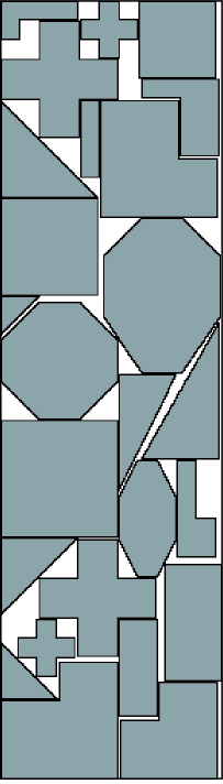
Jakobs1 (88.01%)

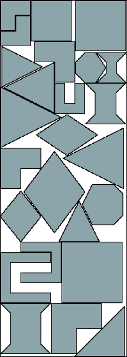
Jakobs2 (79.51%)

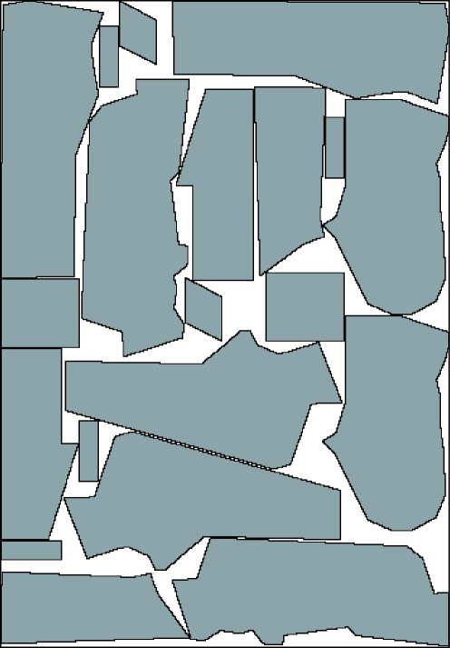
Mao (84.84%)

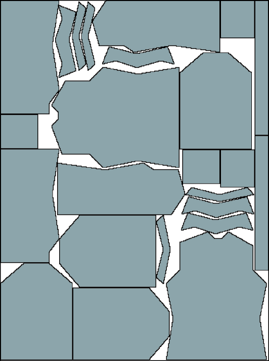
Marques (90.43%)

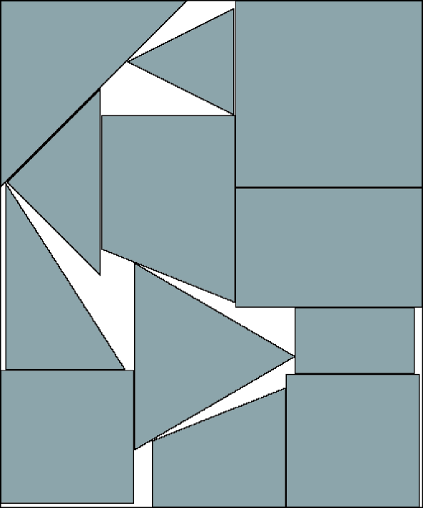
Fu (90.75%)

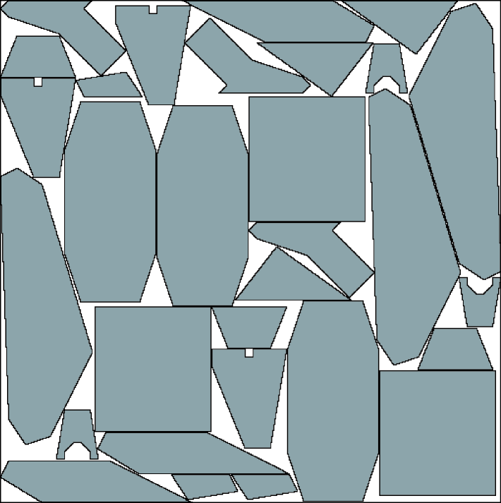
Dagli (86.32%)

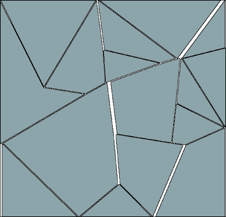
Dighe1 (97.60%)

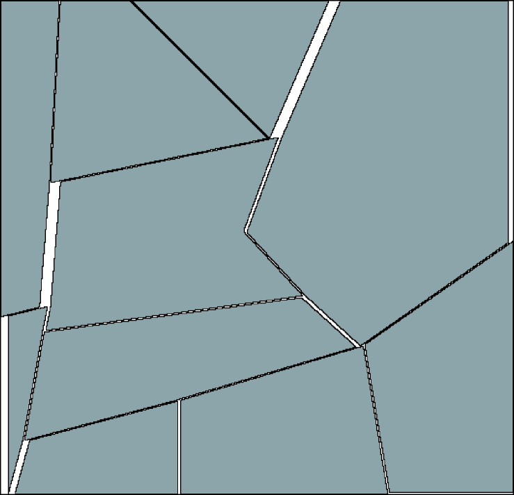
Dighe2 (97.28%)

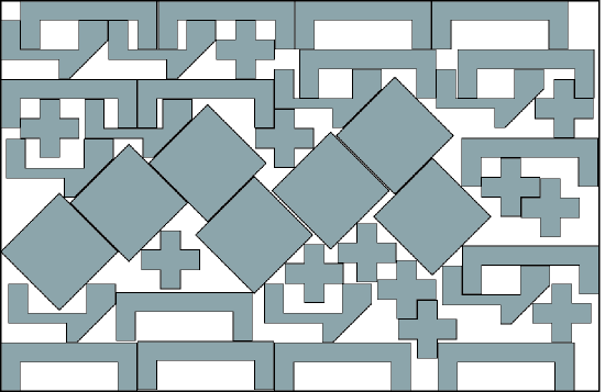
Shapes0 (66.13%)

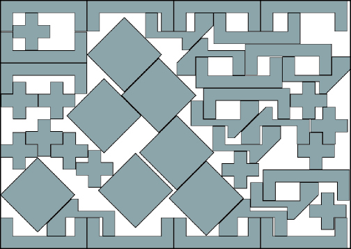
Shapes1 (72.35%)

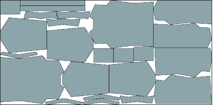
Albano (88.20%)

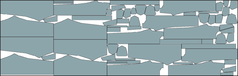
Trousers (88.29%)

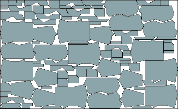
Shirts (84.33%)

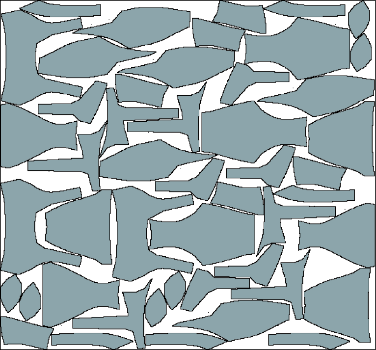
Swim (74.08%)

Figure 17: The best solutions for the test instances obtained by GCDH ($W=512\mathrm{px}$).

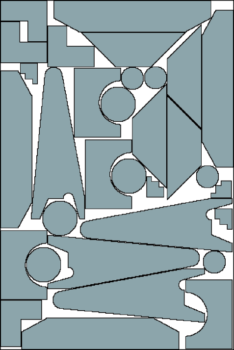
Profiles1 (86.93%)

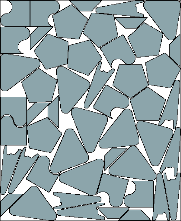
Profiles5 (82.47%)

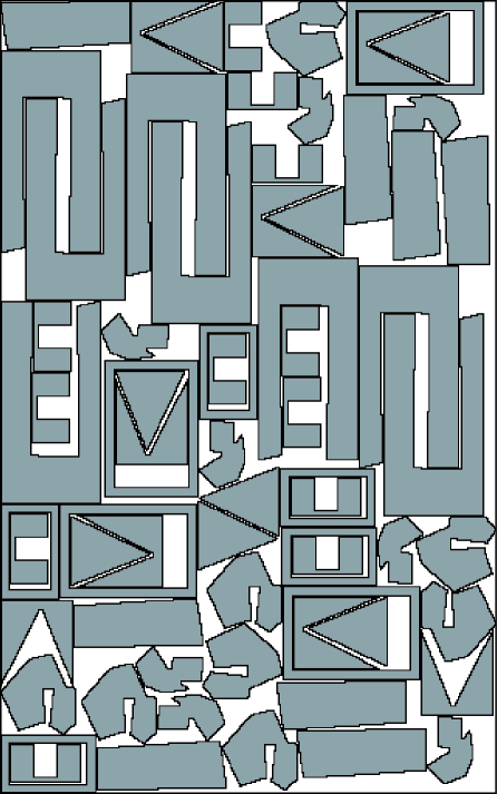
Profiles6 (79.03%)

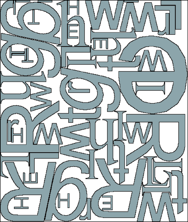
Profiles9 (57.86%)

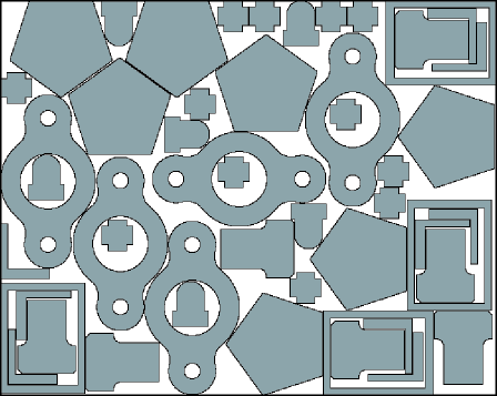
Profiles2 (77.28%)

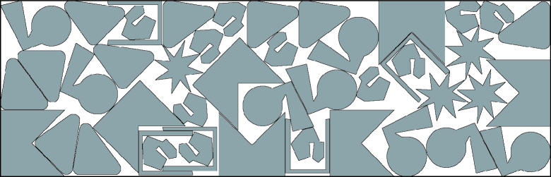
Profiles3 (73.87%)

Profiles7 (95.80%)

Profiles8 (87.61%)

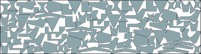
Profiles10 (68.89%)

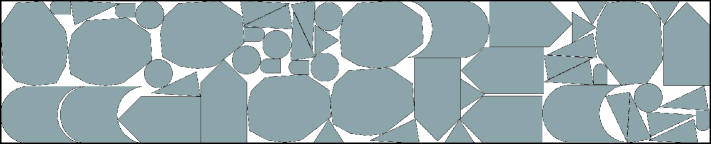
Profiles4 (85.63%)

Figure 18: The best solutions for the test instances obtained by GCDH ($W=512\mathrm{px}$).

We last evaluated the performance of GCDH ($W=512$px) and FITS on large-scale instances that were generated by copying the irregular shapes of the instances Fu and Mao. We tested GCDH and FITS 10 times for each instance with the time limit of 3600 seconds for each run. Table 14 shows the computational results of GCDH and FITS on large-scale instances, which are evaluated in the average density (%) and the number of calls to CDH. The number after the name of each instance shows the number of copies; i.e., “Fu2” contains two copies of every piece in “Fu” and hence the number of pieces is doubled. Figures 19 and 20 also show the number of calls to CDH. The GCDH and FITS take similar tendency in the computational efficiency for the increase of pieces, and their numbers of calls to CDH decrease in proportion to the square of the number of pieces roughly.

Table 14: The computational results of GCDH ($W=512$px) and FITS on large-scale instances (3600 seconds)

			FITS		GCDH
			(vector)		(raster)
instance	#shapes	#pieces	density(%)	#CDHs	density(%)	#CDHs
Fu	11	12	91.98	$3.77\times 10^{6}$	89.78	$2.61\times 10^{6}$
Fu2	11	24	93.70	$1.26\times 10^{6}$	90.77	$7.01\times 10^{5}$
Fu4	11	48	93.49	$4.34\times 10^{5}$	88.81	$1.61\times 10^{5}$
Fu8	11	96	92.43	$1.53\times 10^{5}$	86.81	$3.38\times 10^{4}$
Fu16	11	192	91.78	$4.48\times 10^{4}$	85.66	$6.34\times 10^{3}$
Fu32	11	384	91.80	$1.28\times 10^{4}$	82.12	$8.72\times 10^{2}$
Mao	9	20	84.90	$8.00\times 10^{5}$	84.25	$9.00\times 10^{5}$
Mao2	9	40	84.33	$2.70\times 10^{5}$	82.29	$2.47\times 10^{5}$
Mao4	9	80	82.56	$9.72\times 10^{4}$	80.14	$5.44\times 10^{4}$
Mao8	9	160	81.24	$3.16\times 10^{4}$	79.13	$1.00\times 10^{4}$
Mao16	9	320	80.64	$9.08\times 10^{3}$	78.45	$1.70\times 10^{3}$
Mao32	9	640	80.36	$2.88\times 10^{3}$	76.20	$1.47\times 10^{2}$

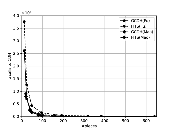
Figure 19: The number of calls to CDH on large-scale instances ($W=512$px) (normal plot)

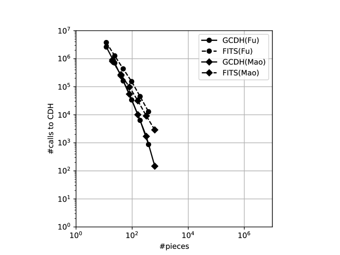
Figure 20: The number of calls to CDH on large-scale instances ($W=512$px) (log-log plot)

7 Conclusion

We develop coordinate descent heuristics for the the irregular strip packing problem (ISP) of the rasterized shapes that repeats a line search in the horizontal and vertical directions alternately. The rasterized shapes provide simple procedures of the intersection test without any exceptional handling due to geometric issues, while they often require much memory and computational effort in high-resolution. To reduce the complexity of rasterized shapes, we first propose the double scanline representation by merging consecutive pixels in each row and column into strips with unit width, respectively. Based on this, we develop an efficient line search algorithm incorporating a corner detection technique used in computer vision to reduce the search space. Computational results for test instances show that the proposed algorithm obtains sufficiently dense layouts of rasterized shapes in high-resolution within a reasonable computation time.

References

- Albano & Sapuppo [1980] Albano, A., & Sapuppo, G. (1980). Optimal allocation of two-dimensional irregular shapes using heuristic search methods. IEEE Transactions on Systems, Man and Cybernetics, 10, 242–248. doi:10.1109/TSMC.1980.4308483.
- Alvarez-Valdes et al. [2018] Alvarez-Valdes, R., Carravilla, M. A., & Oliveira, J. F. (2018). Cutting and packing. In R. Martí, P. M. Pardalos, & M. G. C. Resende (Eds.), Handbook of Heuristics chapter 31. (pp. 931–977). Springer. doi:10.1007/978-3-319-07124-4\_43.
- Art [1966] Art, R. C. (1966). An approach to the two dimensional irregular cutting stock problem. Ph.D. thesis Massachusetts Institute of Technology.
- Babu & Babu [2001] Babu, A. R., & Babu, N. R. (2001). A generic approach for nesting of 2-D parts in 2-D sheets using genetic and heuristic algorithms. Computer-Aided Design, 33, 879–891. doi:10.1016/S0010-4485(00)00112-3.
- Bennell & Dowsland [2001] Bennell, J. A., & Dowsland, K. A. (2001). Hybridising tabu search with optimisation techniques for irregular stock cutting. Management Science, 47, 1160–1172. doi:10.1287/mnsc.47.8.1160.10230.
- Bennell & Oliveira [2008] Bennell, J. A., & Oliveira, J. F. (2008). The geometry of nesting problems: A tutorial. European Journal of Operational Research, 184, 397–415. doi:10.1016/j.ejor.2006.11.038.
- Bennell & Oliveira [2009] Bennell, J. A., & Oliveira, J. F. (2009). A tutorial in irregular shape packing problems. Journal of the Operational Research Society, 60, S93–S105. doi:10.1057/jors.2008.169.
- Bennell & Song [2010] Bennell, J. A., & Song, X. (2010). A beam search implementation for the irregular shape packing problem. Journal of Heuristics, 16, 167–188. doi:10.1007/s10732-008-9095-x.
- Błȧzewicz et al. [1993] Błȧzewicz, J., Hawryluk, P., & Walkowiak, R. (1993). Using a tabu search approach for solving the two-dimensional irregular cutting problem. Annals of Operations Research, 41, 313–325. doi:10.1007/BF02022998.
- Burke et al. [2010] Burke, E. K., Hellier, R. S. R., Kendall, G., & Whitwell, G. (2010). Irregular packing using the line and arc no-fit polygon. Operations Research, 58, 948–970. doi:10.1287/oper.1090.0770.
- Chen et al. [2004] Chen, P., Fu, Z., Lim, A., & Rodrigues, B. (2004). The two-dimensional packing problem for irregular objects. International Journal on Artificial Intelligence Tools, 13, 429–448. doi:10.1142/S0218213004001624.
- Dobkin et al. [1993] Dobkin, D., Hershberger, J., Kirkpatrick, D., & Suri, S. (1993). Computing the intersection-depth of polyhedra. Algorithmica, 9, 518–533. doi:10.1007/BF01190153.
- Dowsland et al. [2002] Dowsland, K. A., Vaid, S., & Dowsland, W. B. (2002). An algorithm for polygon placement using a bottom-left strategy. European Journal of Operational Research, 141, 371–381. doi:10.1016/S0377-2217(02)00131-5.
- Dyckhoff [1990] Dyckhoff, H. (1990). A typology of cutting and packing problems. European Journal of Operational Research, 44, 145–159. doi:10.1016/0377-2217(90)90350-K.
- Egeblad et al. [2007] Egeblad, J., Nielsen, B. K., & Odgaard, A. (2007). Fast neighborhood search for two- and three-dimensional nesting problems. European Journal of Operational Research, 183, 1249–1266. doi:10.1016/j.ejor.2005.11.063.
- Elkeran [2013] Elkeran, A. (2013). A new approach for sheet nesting problem using guided cuckoo search and pairwise clustering. European Journal of Operational Research, 231, 757–769. doi:10.1016/j.ejor.2013.06.020.
- ESICUP [2003] ESICUP (2003). The working group on cutting and packing within EURO. https://www.euro-online.org/websites/esicup/.
- Gomes & Oliveira [2002] Gomes, A. M., & Oliveira, J. F. (2002). A 2-exchange heuristic for nesting problems. European Journal of Operational Research, 141, 359–370. doi:10.1016/S0377-2217(02)00130-3.
- Gomes & Oliveira [2006] Gomes, A. M., & Oliveira, J. F. (2006). Solving irregular strip packing problems by hybridising simulated annealing and linear programming. European Journal of Operational Research, 171, 811–829. doi:10.1016/j.ejor.2004.09.008.
- Hu et al. [2018a] Hu, Y., Fukatsu, S., Imahori, S., & Yagiura, M. (2018a). Efficient overlap detection and construction algorithm for the bitmap shape packing problem. Journal of the Operations Research Society of Japan, 61, 132–150. doi:10.15807/jorsj.61.132.
- Hu et al. [2018b] Hu, Y., Hashimoto, H., Imahori, S., & Yagiura, M. (2018b). Practical algorithms for two-dimensional packing of general shapes. In T. F. Gonzalez (Ed.), Handbook of Approximation Algorithms and Metaheuristics (second edition) chapter 33. (pp. 585–609). CRC Press. doi:10.1201/9781351236423.
- Imamichi et al. [2009] Imamichi, T., Yagiura, M., & Nagamochi, H. (2009). An iterated local search algorithm based on nonlinear programming for the irregular strip packing problem. Discrete Optimization, 6, 345–361. doi:10.1016/j.disopt.2009.04.002.
- Jain & Gea [1998] Jain, S., & Gea, C. (1998). Two-dimensional packing problems using genetic algorithms. Engineering with Computers, 14, 206–213. doi:10.1115/96-DETC/DAC-1466.
- Leao et al. [2020] Leao, A. A. S., Toledo, F. M. B., Oliveira, J. F., Carravilla, M. A., & Alvarez-Valdés, R. (2020). Irregular packing problems: A review of mathematical models. European Journal of Operational Research, 282, 803–822. doi:10.1016/j.ejor.2019.04.045.
- Leung et al. [2012] Leung, S. C. H., Lin, Y., & Zhang, D. (2012). Extended local search algorithm based on nonlinear programming for two-dimensional irregular strip packing problem. Computers & Operations Research, 39, 678–686. doi:10.1016/j.cor.2011.05.025.
- Li & Milenkovic [1995] Li, Z., & Milenkovic, V. (1995). Compaction and separation algorithms for non-convex polygons and their applications. European Journal of Operational Research, 84, 539–561. doi:10.1016/0377-2217(95)00021-H.
- Mundim et al. [2017] Mundim, L. R., Andretta, M., & de Queiroz, T. A. (2017). A biased random key genetic algorithm for open dimensional nesting problems using no-fit raster. Expert Systems with Applications, 81, 358–371. doi:10.1016/j.eswa.2017.03.059.
- Okano [2002] Okano, H. (2002). A scanline-based algorithm for the 2D free-form bin packing problem. Journal of the Operations Research Society of Japan, 45, 145–161. doi:10.15807/jorsj.45.145.
- Oliveira & Ferreira [1993] Oliveira, J. F., & Ferreira, J. S. (1993). Algorithms for nesting problems. In R. V. V. Vaidel (Ed.), Applied Simulated Annealing (Lecture Notes in Economics and Maths Systems) (pp. 255–274). Springer volume 396. doi:10.1007/978-3-642-46787-5\_13.
- Oliveira et al. [2000] Oliveira, J. F., Gomes, A. M., & Ferreira, J. S. (2000). Topos — a new constructive algorithm for nesting problems. OR Spectrum, 22, 263–284. doi:10.1007/s002910050105.
- Rosten & Drummond [2006] Rosten, E., & Drummond, T. (2006). Machine learning for high-speed corner detection. In European Conference on Computer Vision (pp. 430–443). doi:10.1007/11744023\_34.
- Sato et al. [2019] Sato, A. K., Martins, T. C., Gomes, A. M., & Tsuzuki, M. S. G. (2019). Raster penetration map applied to the irregular packing problem. European Journal of Operational Research, 279, 657–671. doi:10.1016/j.ejor.2019.06.008.
- Scheithauer [2018] Scheithauer, G. (2018). Introduction to Cutting and Packing Optimization. Springer. doi:10.1007/978-3-319-64403-5.
- Segenreich & Braga [1986] Segenreich, S. A., & Braga, L. M. P. F. (1986). Optimal nesting of general plane figures: A monte carlo heuristical approach. Computers & Graphics, 10, 229–237. doi:10.1016/0097-8493(86)90007-5.
- Toledo et al. [2013] Toledo, F. M. B., Carravilla, M. A., Ribeiro, C., & Oliveira, J. F. (2013). The dotted-board model: A new mip model for nesting irregular shapes. International Journal of Production Economics, 145, 478–487. doi:10.1016/j.ijpe.2013.04.009.
- Umetani et al. [2009] Umetani, S., Yagiura, M., Imahori, S., Imamichi, T., Nonobe, K., & Ibaraki, T. (2009). Solving the irregular strip packing problem via guided local search for overlap minimization. International Transactions in Operational Research, 16, 661–683. doi:10.1111/j.1475-3995.2009.00707.x.
- Voudouris & Tsang [1999] Voudouris, C., & Tsang, E. (1999). Guided local search and its application to the traveling salesman problem. European Journal of Operational Research, 113, 469–499. doi:10.1016/S0377-2217(98)00099-X.
- Wäscher et al. [2007] Wäscher, G., Haußner, H., & Schumann, H. (2007). An improved typology of cutting and packing problems. European Journal of Operational Research, 183, 1109–1130. doi:10.1016/j.ejor.2005.12.047.
- Wong et al. [2009] Wong, W. K., Wang, X. X., Mok, P. Y., Leung, S. Y. S., & Kwong, C. K. (2009). Solving the two-dimensional irregular objects allocation problems by using a two-stage packing approach. Expert Systems with Applications, 36, 3489–3496. doi:10.1016/j.eswa.2008.02.068.