Relating Adversarially Robust Generalization to Flat Minima

Abstract

Adversarial training (AT) has become the de-facto standard to obtain models robust against adversarial examples. However, AT exhibits severe robust overfitting: cross-entropy loss on adversarial examples, so-called robust loss, decreases continuously on training examples, while eventually increasing on test examples. In practice, this leads to poor robust generalization, i.e., adversarial robustness does not generalize well to new examples. In this paper, we study the relationship between robust generalization and flatness of the robust loss landscape in weight space, i.e., whether robust loss changes significantly when perturbing weights. To this end, we propose average- and worst-case metrics to measure flatness in the robust loss landscape and show a correlation between good robust generalization and flatness. For example, throughout training, flatness reduces significantly during overfitting such that early stopping effectively finds flatter minima in the robust loss landscape. Similarly, AT variants achieving higher adversarial robustness also correspond to flatter minima. This holds for many popular choices, e.g., AT-AWP, TRADES, MART, AT with self-supervision or additional unlabeled examples, as well as simple regularization techniques, e.g., AutoAugment, weight decay or label noise. For fair comparison across these approaches, our flatness measures are specifically designed to be scale-invariant and we conduct extensive experiments to validate our findings.

1 Introduction

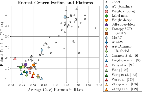
Figure 1: Robust Generalization and Flatness: Robust loss (RLoss , lower is more robust, y-axis), i.e., cross-entropy loss on PGD adversarial examples [81], against our average-case flatness measure of RLoss in weight space (lower is “flatter”, x-axis). Popular AT variants improving adversarial robustness on CIFAR10, e.g., TRADES [148], AT-AWP [133], MART [128] or AT with self-supervision [50]/unlabeled examples [16], also correspond to flatter minima. Vice-versa, regularization explicitly improving flatness, e.g., Entropy-SGD [17], weight decay or weight clipping [117], also improve robustness. Across all models, there is a clear relationship between good robust generalization and flatness in RLoss . $\bullet$,$\mathbin{\blacklozenge}$ Our models, w/o early stopping. $\blacktriangle$ RobustBench [24] models w/ early stopping.

In order to obtain robustness against adversarial examples [123], adversarial training (AT) [81] augments training with adversarial examples that are generated on-the-fly. While many different variants have been proposed, AT is known to require more training data [63, 108], generally leading to generalization problems [37]. In fact, robust overfitting [103] has been identified as the main problem in AT: adversarial robustness on test examples eventually starts to decrease, while robustness on training examples continues to increase (cf. Fig. 2). This is typically observed as increasing robust loss (RLoss ) or robust test error (RErr ), i.e., (cross-entropy) loss and test error on adversarial examples. As a result, the robust generalization gap, i.e., the difference between test and training robustness, tends to be very large. In [103], early stopping is used as a simple and effective strategy to avoid robust overfitting. However, despite recent work tackling robust overfitting [114, 133, 53], it remains an open and poorly understood problem.

In “clean” generalization (i.e., on natural examples), overfitting is well-studied and commonly tied to flatness of the loss landscape in weight space, both visually [73] and empirically [91, 62, 60]. In general, the optimal weights on test examples do not coincide with the minimum found on training examples. Flatness ensures that the loss does not increase significantly in a neighborhood around the found minimum. Therefore, flatness leads to good generalization because the loss on test examples does not increase significantly (i.e., small generalization gap, cf. Fig. 3, right). [73] showed that visually flatter minima correspond to better generalization. [91] and [62] formalize this idea by measuring the change in loss within a local neighborhood around the minimum considering random [91] or “adversarial” weight perturbations [62]. These measures are shown to be effective in predicting generalization in a recent large-scale empirical study [60] and explicitly encouraging flatness during training has been shown to be successful in practice [151, 21, 75, 17, 57].

Recently, [133] applied the idea of flat minima to AT: through adversarial weight perturbations, AT is regularized to find flatter minima of the robust loss landscape. This reduces the impact of robust overfitting and improves robust generalization, but does not avoid robust overfitting. As result, early stopping is still necessary. Furthermore, flatness is only assessed visually and it remains unclear whether flatness does actually improve in these adversarial weight directions. Similarly, [42] shows that weight averaging [57] can improve robust generalization, indicating that flatness might be beneficial in general. This raises the question whether other “tricks” [92, 42], e.g., different activation functions [114] or label smoothing [121], or approaches such as AT with self-supervision [50]/unlabeled examples [16] are successful because of finding flatter minima.

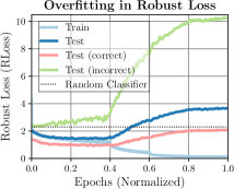
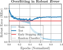
Figure 2: Robust Overfitting: Robust (cross-entropy) loss (RLoss ) and robust error (RErr ) over epochs (normalized by $150$ epochs) for AT, using a ResNet-18 on CIFAR10 (cf. Sec. 4), to illustrate robust overfitting. Left: Training RLoss (light blue) reduces continuously throughout training, while test RLoss (dark blue) eventually increases again. We also highlight that robust overfitting is not limited to incorrectly classified examples (green), but also affects correctly classified ones (rose). Right: Similar behavior, but less pronounced, can be observed considering RErr . We also show RErr obtained through early stopping (red).

Contributions: In this paper, we study whether flatness of the robust loss (RLoss ) in weight space improves robust generalization. To this end, we propose both average- and worst-case flatness measures for the robust case, thereby addressing challenges such as scale-invariance [31], estimation of RLoss on top or jointly with weight perturbations, and the discrepancy between RLoss and RErr . We show that robust generalization generally improves alongside flatness and vice-versa: Fig. 1 plots RLoss (lower is more robust, y-axis) against our average-case flatness in RLoss (lower is flatter, x-axis), showing a clear relationship. In contrast to [133], not providing empirical flatness measures, our results show that this relationship is stronger for average-case flatness. This trend covers a wide range of AT variants on CIFAR10, e.g., AT-AWP [133], TRADES [148], MART [128], AT with self-supervision [50] or additional unlabeled examples [16, 2], as well as various regularization schemes, including AutoAugment [27], label smoothing [121] and noise or weight clipping [117]. Furthermore, we consider hyper-parameters, e.g., learning rate schedule, weight decay, batch size, or different activation functions [35, 85, 49], and methods explicitly improving flatness, e.g., Entropy-SGD [17] or weight averaging [57].

2 Related Work

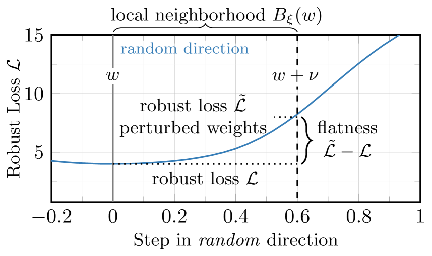
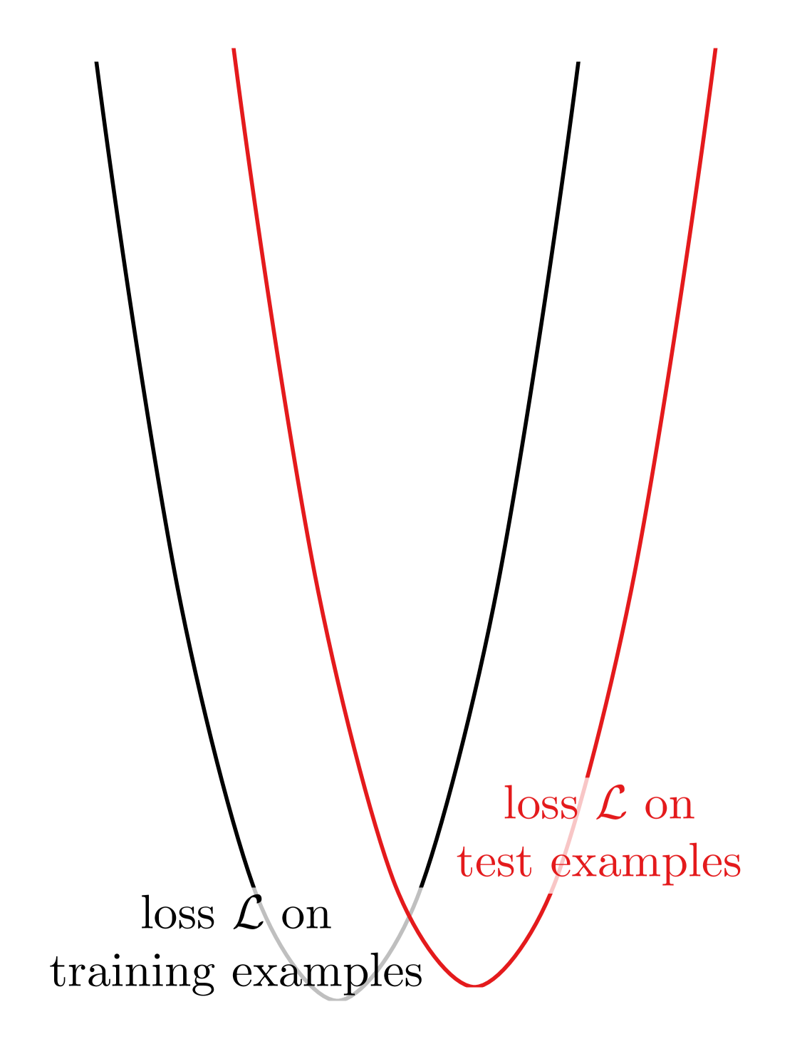
Figure 3: Measuring Flatness. Left: Illustration of measuring flatness in a random (i.e., average-case, blue) direction by computing the difference between RLoss $\tilde{\mathcal{L}}$ after perturbing weights (i.e., $w+\nu$) and the “reference” RLoss $\mathcal{L}$ given a local neighborhood $B_{\xi}(w)$ around the found weights $w$, see Sec. 3.3. In practice, we average across/take the worst of several random/adversarial directions. Right: Large changes in RLoss around the “sharp” minimum causes poor generalization from training (black) to test examples (red).

Adversarial Training (AT): Despite a vast amount of work on adversarial robustness, e.g., see [111, 142, 1, 9, 137], adversarial training (AT) has become the de-facto standard for (empirical) robustness. Originally proposed in different variants in [123, 86, 52], it received considerable attention in [81, 36] and has been extended in various ways: [71, 16, 2] utilize interpolated or unlabeled examples, [125, 82] achieve robustness against multiple threat models, [119, 69, 135] augment AT with a reject option, [140, 77] use Bayesian networks, [126, 43] build ensembles, [7, 30] adapt the threat model for each example, [131, 4, 105] perform AT with single-step attacks, [50] uses self-supervision and [93] additionally regularizes features – to name a few directions. However, AT is slow [145] and suffers from increased sample complexity [108] as well as reduced (clean) accuracy [127, 118, 148, 100]. Furthermore, progress is slowing down. In fact, “standard” AT is shown to perform surprisingly well on recent benchmarks [25, 24] when tuning hyper-parameters properly [92, 42]. In our experiments, we consider several popular variants [133, 128, 148, 16, 50].

Robust Overfitting: Recently, [103] identified robust overfitting as a crucial problem in AT and proposed early stopping as an effective mitigation strategy. This motivated work [114, 133] trying to mitigate robust overfitting. While [114] studies the use of different activation functions, [133] proposes AT with adversarial weight perturbations (AT-AWP) explicitly aimed at finding flatter minima in order to reduce overfitting. While the results are promising, early stopping is still necessary. Furthermore, flatness is merely assessed visually, leaving open whether AT-AWP actually improves flatness in adversarial weight directions. We consider both average- and worst-case flatness, i.e., random and adversarial weight perturbations, to answer this question.

Flat Minima in the loss landscape, w.r.t. changes in the weights, are generally assumed to improve standard generalization [51]. [73] shows that residual connections in ResNets [45] or weight decay lead to visually flatter minima. [91, 62] formalize this concept of flatness in terms of average-case and worst-case flatness. [62, 60] show that worst-case flatness correlates well with better generalization, e.g., for small batch sizes, while [91] argues that generalization can be explained using both an average-case flatness measure and an appropriate capacity measure. Similarly, batch normalization is argued to improve generalization by allowing to find flatter minima [106, 10]. These insights have been used to explicitly regularize flatness [151], improve semi-supervised learning [21] and develop novel optimization algorithms such as Entropy-SGD [17], local SGD [75] or weight averaging [57]. [31], in contrast, criticizes some of these flatness measures as not being scale-invariant. We transfer the intuition of flatness to the robust loss landscape, showing that flatness is desirable for adversarial robustness, while using scale-invariant measures.

3 Robust Generalization and Flat Minima

Model	RErr $\downarrow$
AT (baseline) $\bullet$	62.8
Scaled $\times 0.5$ $\bullet$	62.8
Scaled $\times 2$ $\bullet$	62.8
MiSH $\bullet$	59.8
Batch size $8$ $\bullet$	58.2
Adam $\bullet$	57.5
Label smoothing $\bullet$	61.2
MART $\bullet$	61
Entropy-SGD $\bullet$	58.6
Self-supervision $\bullet$	57.1
TRADES $\bullet$	56.7
AT-AWP $\bullet$	54.3

 

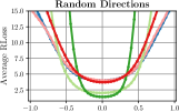
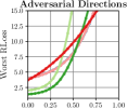
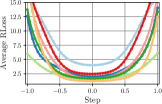
Figure 4: Visualizing Flatness: RLoss landscape across $10$ random or adversarial directions. Top: Our AT baseline (ResNet-18) and scaled variants ($\times 2$ and $\times 0.5$). Training with smaller batch size or Adam [64] improves adversarial robustness (lower RErr vs. AutoAttack [25]) but does not result in visually flatter minima. Bottom: AT-AWP [133] or Entropy-SGD [17] improve robustness and visual flatness in random directions. In adversarial directions, however, AT-AWP looks very sharp. Overall, visual inspection does not provide a clear, objective picture of flatness.

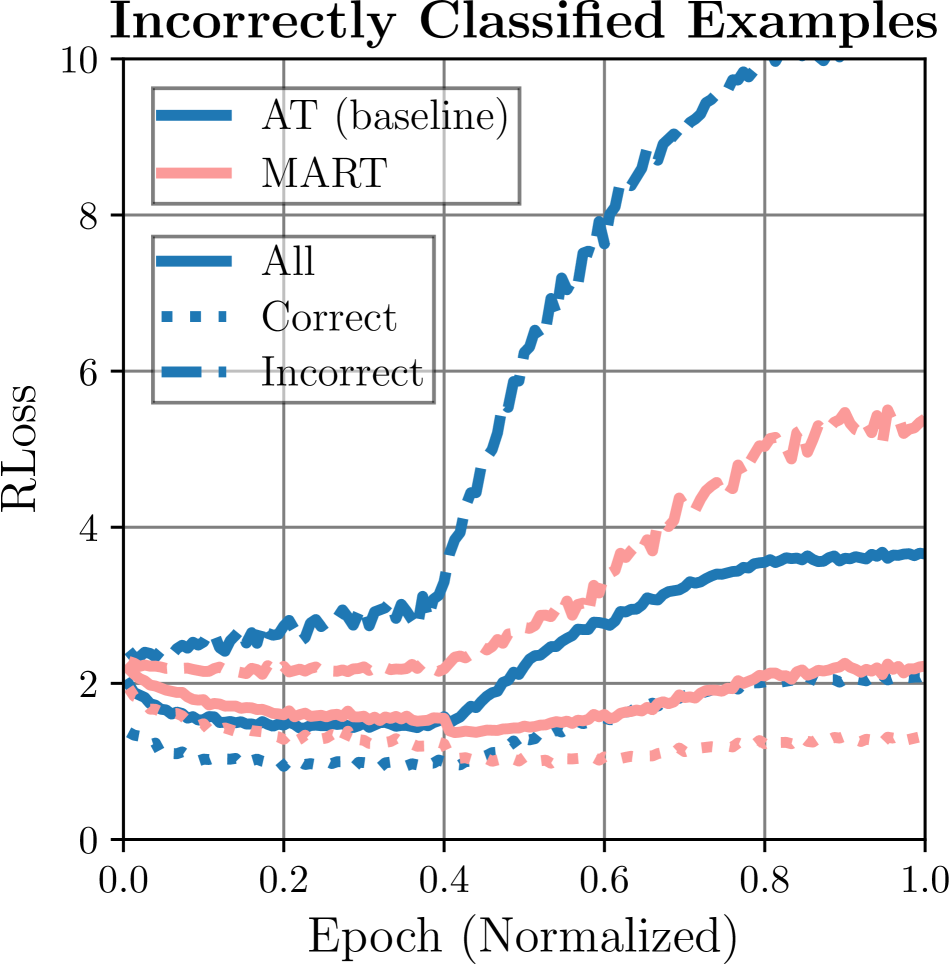
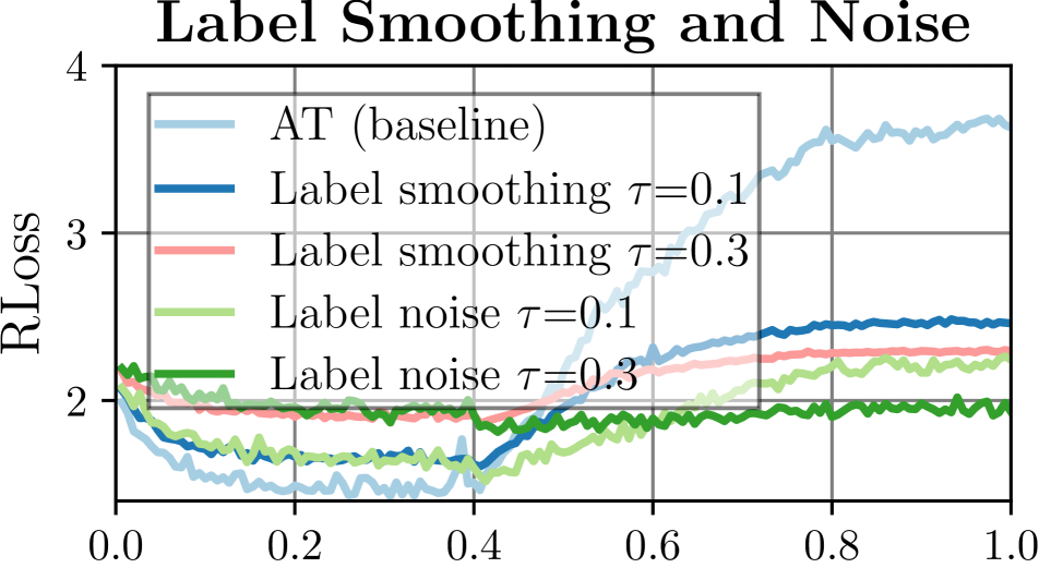
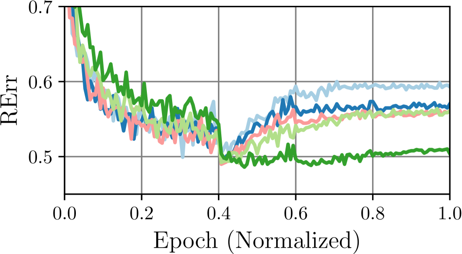
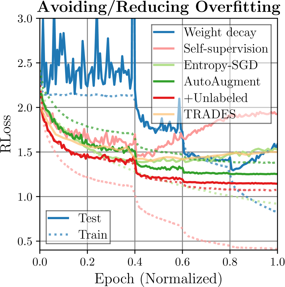
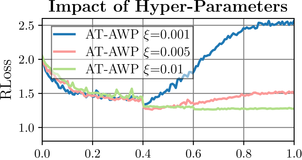
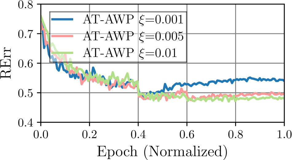
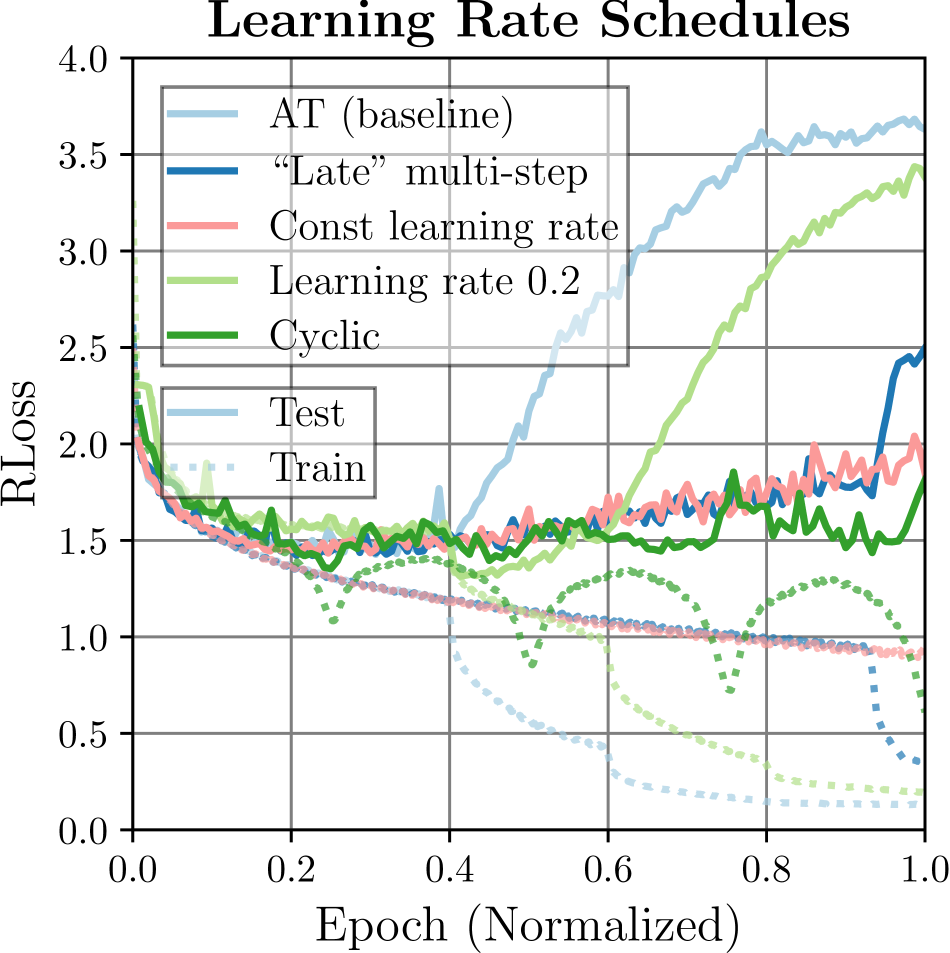
Figure 5: Understanding Robust Overfitting: Training curves plotted over (normalized) epochs, see Sec. 3.4 for detailed discussion. First column: RLoss , split for correct/incorrect test examples, for AT and MART, which successfully dampens the effect of overfitting using a weighted loss on incorrectly classified examples. Second column: Both label smoothing and label noise reduce robust overfitting w.r.t. RLoss . However, the reduction in RLoss does not translate to a similar reduction of RErr . Third to fifth column: RLoss (test solid and train dotted) for various approaches improving adversarial robustness and different learning rate schedules. While some approaches avoid robust overfitting altogether (e.g., AT-AWP), others (e.g., weight decay) merely reduce its impact (third column). But the success depends strongly on hyper-parameters (fourth column). Robust overfitting occurs using all tested learning rate schedules (fifth column), confirming [103].

We study robust generalization and overfitting in the context of flatness of the robust loss landscape in weight space, i.e., w.r.t. changes in the weights. While flat minima have consistently been linked to standard generalization [51, 73, 91, 62], this relationship remains unclear for adversarial robustness. We start by briefly introducing the robust overfitting phenomenon (Sec. 3.1). Then, we discuss problems in judging flatness visually [73] (Sec. 3.2). Thus, we are inspired by [62, 91] and introduce average- and worst-case flatness measures based on the change in robust loss along random or adversarial weight directions in a local neighborhood (Sec. 3.3), cf. Fig. 3. We also discuss the connection of flatness to the Hessian eigenspectrum [139] and the importance of scale-invariance as in [31].

3.1 Background

Adversarial Training (AT): Let $f$ be a (deep) neural network taking input $x\in[0,1]^{D}$ and weights $w\in\mathbb{R}^{W}$ and predicting a label $f(x;w)$. Given a true label $y$, an adversarial example is a perturbation $\tilde{x}=x+\delta$ such that $f(\tilde{x};w)\neq y$. The perturbation $\delta$ is intended to be nearly invisible which is, in practice, enforced using a $L_{p}$ constraint: $\|\delta\|_{p}\leq\epsilon$. To obtain robustness against these perturbations, AT injects adversarial examples during training:

$$\mathop{\rm min}\nolimits_{w}\mathbb{E}_{x,y}\left[\mathop{\rm max}\nolimits_{\|\delta\|_{p}\leq\epsilon}\mathcal{L}(f(x+\delta;w),y)\right]$$ (1)

where $\mathcal{L}$ denotes the cross-entropy loss. The outer minimization problem can be solved using regular stochastic gradient descent (SGD) on mini-batches. To compute adversarial examples, the inner maximization problem is tackled using projected gradient descent (PGD) [81]. Here, we focus on $p=\infty$ as this constrains the maximum change per feature/pixel, e.g., $\epsilon=\nicefrac{{8}}{{255}}$ on CIFAR10. For evaluation (at test time), we consider both robust loss (RLoss ) $\mathop{\rm max}\nolimits_{\|\delta\|_{\infty}\leq\epsilon}\mathcal{L}(f(x+\delta;w),y)$, approximated using PGD, and robust test error (RErr ), which we approximate using AutoAttack [25]. Note that AutoAttack stops when adversarial examples are found and does not maximize cross-entropy loss, rendering it unfit to estimate RLoss .

Robust Overfitting: Following [103], Fig. 2 illustrates the problem of robust overfitting, plotting RLoss (left) and RErr (right) over epochs, which we normalize by the total number of epochs for clarity. Shortly after the first learning rate drop (at epoch $60$, i.e., $40\%$ of training), test RLoss and RErr start to increase significantly, while robustness on training examples continues to improve. Robust overfitting was shown to be independent of the learning rate schedule [103] and, as we show (Sec. 4.1), occurs across various different activation functions as well as many popular AT variants. In contrast to [103], mostly focusing on RErr , Fig. 2 shows that RLoss overfits more severely, indicating a “disconnectedness” between RLoss and RErr that we consider in detail later. For now, RLoss and RErr do clearly not move “in parallel” and RLoss , reaching values around $4$, is higher than for a random classifier (which is possible considering adversarial examples). This is primarily due to an extremely high RLoss on incorrectly classified test examples (which are “trivial” adversarial examples). We emphasize, however, that robust overfitting also occurs on correctly classified test examples.

3.2 Intuition and Visualizing Flatness

 

 

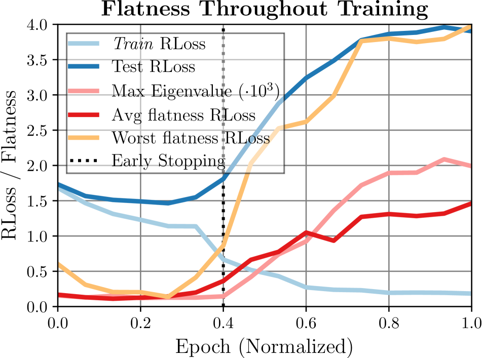
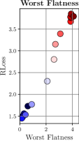
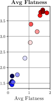
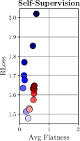
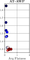
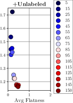
Figure 6: Flatness Throughout Training. Left: Flatness in RLoss throughout training, showing that flatness reduces when the model overfits (i.e., test RLoss increases, while train RLoss decreases). Middle: Test RLoss (y-axis) plotted against flatness in RLoss (x-axis) during training (early epochs in dark blue, late epochs in dark red), showing a clear correlation, for both average- and worst-case flatness. Right: AT with self-supervision reduces the impact of robust overfitting (RLoss increases less) and simultaneously favors flatter minima. This behavior is pronounced for AT-AWP, explicitly optimizing flatness, and AT with additional unlabeled examples, generally resulting in the highest adversarial robustness, cf. Tab. 1.

For judging robust flatness, we consider how RLoss changes w.r.t. random or adversarial perturbations in the weights $w$. Generally, we expect flatter minima to generalize better as the loss does not change significantly within a small neighborhood around the minimum, i.e., the found weights. Then, even if the loss landscape on test examples does not coincide with the loss landscape on training examples, loss remains small, ensuring good generalization. The contrary case, i.e., that sharp minima generalize poorly is illustrated in Fig. 3 (right). Before considering to measure flatness, we discuss the easiest way to “judge” flatness: visual inspection of the RLoss landscape along random or adversarial directions in weight space.

In [73], loss landscape is visualized along normalized random directions. Normalization is important to handle different scales, i.e., weight distributions, and allow comparison across models. We follow [133] and perform per-layer normalization: Letting $\nu\in\mathbb{R}^{W}$ be a direction in weight space, it is normalized as

$$\hat{\nu}^{(l)}=\frac{\nu^{(l)}}{\|\nu^{(l)}\|_{2}}\|w^{(l)}\|_{2}\quad\text{ for layer }l.$$ (2)

In contrast to [73], we also consider biases and treat them as individual layer, but we exclude batch normalization parameters. Then, the loss landscape is visualized in discrete steps along this direction, i.e., $w+s\hat{\nu}$ for $s\in[-1,1]$. Adversarial examples are computed “on-the-fly”, i.e., for each $w+s\hat{\nu}$ individually, to avoid underestimating RLoss as in [141, 97]. The result is indeed scale-invariant: Fig. 4 (top) shows that the loss landscapes for scaled versions (factors $0.5$ or $2$, see supplementary material) of our AT baseline coincide with the original landscape. However, Fig. 4 also illustrates that judging flatness visually is difficult: Considering random weight directions, AT with Adam [64] or small batch size improves adversarial robustness, but the found minima look less flat (top). For other approaches, e.g., TRADES [148] or AT-AWP [133], results look indeed flatter while also improving robustness (bottom). In adversarial directions, in contrast, AT-AWP looks particularly sharp. Furthermore, not only flatness but also the vertical “height” of the loss landscape matters and it is impossible to tell “how much” flatness is necessary.

3.3 Average- and Worst-Case Flatness Measures

In order to objectively measure and compare flatness, we draw inspiration from [91, 62] and propose average- and worst-case flatness measures adapted to the robust loss. We emphasize that measuring flatness in RLoss is non-trivial and flatness in (clean) Loss cannot be expected to correlate with robustness (see supplementary material). For example, we need to ensure scale-invariance [31] and estimate RLoss on top of random or adversarial weight perturbations:

Average-Case / Random Flatness: Considering random weight perturbations $\nu\in B_{\xi}(w)$ within the $\xi$-neighborhood of $w$, average-case flatness is computed as

$$\begin{split}\mathbb{E}_{\nu}[\mathop{\rm max}\nolimits\limits_{\|\delta\|_{\infty}\leq\epsilon}\mathcal{L}(f(x{+}\delta;w{+}\nu),y)]\text{\hphantom{aaaaaaaaaaa}}\\[-2.00749pt] \text{\hphantom{aaaaaaaaaaa}}-\mathop{\rm max}\nolimits\limits_{\|\delta\|_{\infty}\leq\epsilon}\mathcal{L}(f(x{+}\delta;w),y)\end{split}$$ (3)

averaged over test examples $x,y$, as illustrated in Fig. 3. We define $B_{\xi}(w)$ using relative $L_{2}$-balls per layer (cf. Eq. (2)):

$$B_{\xi}(w)=\{w+\nu:\|\nu^{(l)}\|_{2}\leq\xi\|w^{(l)}\|_{2}\forall\text{ layers }l\}.$$ (4)

This ensures scale-invariance w.r.t. the weights as $B_{\xi}(w)$ scales with the weights on a per-layer basis. Note that the second term in Eq. (3), i.e., the “reference” robust loss, is important to make the measure independent of the absolute loss (i.e., corresponding to the vertical shift in Fig. 4, left). In practice, $\xi$ can be as large as $0.5$. We refer to Eq. (3) as average-case flatness in RLoss .

Worst-Case / Adversarial Flatness: [133] explicitly optimizes flatness in adversarial weight directions and shows that average-case flatness is not sufficient to improve adversarial robustness. As it is unclear whether [133] actually improves worst-case flatness, we define

$$\begin{split}\mathop{\rm max}\nolimits\limits_{\nu\in B_{\xi}(w)}&\left[\mathop{\rm max}\nolimits\limits_{\|\delta\|_{\infty}\leq\epsilon}\mathcal{L}(f(x{+}\delta;w{+}\nu),y)\right]\hphantom{aaaaaa}\\[1.00374pt] &\hphantom{aaaaaaaa}-\mathop{\rm max}\nolimits\limits_{\|\delta\|_{\infty}\leq\epsilon}\mathcal{L}(f(x{+}\delta;w),y)\end{split}$$ (5)

as worst-case flatness in RLoss . Here, we use the same definition of $B_{\xi}(w)$ as above (aligned with [133]), but for smaller values of $\xi$. Regarding standard performance, this worst-case notion of flatness has been shown to be a reliable predictor of generalization [60, 62]. For computing Eq. (5) in practice, we jointly optimize over $\nu$ and $\delta$ (for each batch individually) using PGD. As illustrated in Fig. 4, RLoss increases quickly along adversarial directions, even for very small values of $\xi$, e.g., $\xi=0.005$.

3.4 Discussion

In the context of flatness, there has also been some discussion concerning the meaning of Hessian eigenvalues [73, 139] as well as concerns regarding the scale-invariance of flatness measures [31]. First, regarding the Hessian eigenspectrum, [139] shows that large Hessian eigenvalues indicate poor adversarial robustness. However, Hessian eigenvalues are generally not scale-invariant (which is acknowledged in [139]): Our AT baseline has a maximum eigenvalue of $1990$ which reduces to $505$ when up-scaling the model and increases to $7936$ when down-scaling, without affecting robustness (cf. $\times 0.5$ and $\times 2$ in Fig. 4). We also found that the largest eigenvalue is not correlated with adversarial robustness. Second, following a similar train of thought, [31] criticizes the flatness measures of [91, 62] as not being scale-invariant. That is, through clever scaling of weights, without changing predictions, arbitrary flatness values can be “produced”. However, the analysis in [31] does not take into account the relative neighborhood as defined in [62], which renders the measure explicitly scale-invariant. This also applies to our definition of $B_{\xi}(w)$ in Eq. (4) and is shown in Fig. 4 where normalization is performed relative (per-layer) to the weights; empirical validation can be found in the supplementary material.

4 Experiments

We start with a closer look at RLoss in robust overfitting (Sec. 4.1, Fig. 5). Then, we show a strong correlation between good robust generalization and flatness (Sec. 4.2). For example, robust overfitting causes sharper minima (Fig. 6). More importantly, more robust models generally find flatter minima and, vice-versa, methods encouraging flatness improve adversarial robustness (Fig. 7, 8). In fact, flatness improves robust generalization by both lowering the robust generalization gap (incl. a reduction in robust overfitting, cf. Fig. 9).

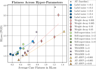
Figure 7: Flatness Across Hyper-Parameters: RLoss (y-axis) vs. average-case flatness (x-axis) for selected methods and hyper-parameters (cf. supplementary material). For example, we consider different strengths of weight decay (rose) or sizes $\xi$ of adversarial weight perturbations for AT-AWP (orange). For clarity, we plot (dotted) lines representing the trend per method. Clearly, improved adversarial robustness, i.e., low RLoss , is related to improved flatness.

Setup: On CIFAR10 [65], our AT baseline uses ResNet-18 [45] and is trained for $150$ epochs, batch size $128$, learning rate $0.05$, reduced by factor $0.1$ at $60$, $90$ and $120$ epochs, using weight decay $0.005$ and momentum $0.9$ with standard SGD. We use random flips and cropping as data augmentation. During training, we use $7$ iterations PGD, with learning rate $0.007$, signed gradient and $\epsilon=\nicefrac{{8}}{{255}}$ for $L_{\infty}$ adversarial examples. PGD-$7$ is also used for early stopping (every $5$th epoch) on the last $500$ test examples. We do not use early stopping by default. For evaluation on the first $1000$ test examples, we run PGD with $20$ iterations, $10$ random restarts to estimate RLoss and AutoAttack [25] to estimate RErr (cf. Sec. 3.1). For average-case flatness of RLoss , we take the average of $10$ random weight perturbations with $\xi{=}0.5$. For worst-case flatness, we maximize RLoss jointly over adversarial examples and adversarial weights with $\xi{=}0.00075$, taking the worst of $10$ restarts.

Methods: Besides our AT baseline, we consider AT-AWP [134], TRADES [148], MART [128], AT with self-supervision [50] or additional unlabeled examples [16, 2], weight averaging [57] and AT with “early-stopped” PGD [149]. We investigate different hyper-parameters and “tricks” recently studied in [92, 42]: learning rate schedules, batch size, weight decay, label smoothing [121] as well as SiLU/Mish/GeLU [35, 85, 49] activation functions. Furthermore, we consider Entropy-SGD [17], label noise, weight clipping [117] and AutoAugment [27]. We emphasize that weight averaging, Entropy-SGD and weight clipping are known to improve flatness of the (clean) loss. If not stated otherwise, these methods are applied on top or as replacement of our AT baseline. We report results using the best hyper-parameters per method. Finally, we also use pre-trained models from RobustBench [24], which were obtained using early stopping.

Model	Robustness $\downarrow$		Flatness $\downarrow$		Early Stop.
(sorted asc. by test RErr )	RErr	RErr	Avg	Worst	RErr $\downarrow$
(split at $70\%$/$30\%$ percentiles)	(test)	(train)	(RLoss )	(RLoss )	(early stop)
+Unlabeled	48.9	43.2 (-5.7)	0.32	1.20	48.9 (-0.0)
Cyclic	53.6	35.4 (-18.2)	0.35	1.50)	53.6 (-0.0)
AutoAugment	54.0	47.9 (-6.1)	0.49	0.69	53.5 (-0.5)
AT-AWP	54.3	43.1 (-11.2)	0.35	2.68	53.6 (-0.7)
Label noise	56.2	30.0 (-26.2)	0.33	0.93)	55.5 (-0.7)
Weight clipping	56.5	39.0 (-17.5)	0.41	4.57	56.5 (-0.0)
TRADES	56.7	15.8 (-40.9)	0.57	2.25	53.4 (-3.3)
Self-supervision	57.1	45.0 (-12.1)	0.33	2.63	56.8 (-0.3)
Weight decay	58.1	32.8 (-25.3)	0.50	3.93	54.8 (-3.3)
Entropy-SGD	58.6	46.1 (-12.5)	0.28	1.80	56.9 (-1.7)
MiSH	59.8	5.3 (-54.5)	1.56	3.54	53.7 (-6.1)
“Late” multi-step	59.8	18.4 (-41.4)	0.80	2.96	57.8 (-2.0)
SiLU	60.0	5.6 (-54.4)	1.71	4.20	53.7 (-6.3)
Weight averaging	60.0	10.0 (-50.0)	1.28	5.98	53.0 (-7.0)
Larger $\epsilon{=}\nicefrac{{9}}{{255}}$	60.9	11.1 (-49.8)	1.33	5.84	53.8 (-7.1)
MART	61.0	20.8 (-40.2)	0.73	3.17	54.7 (-6.3)
GeLU	61.1	3.2 (-57.9)	1.55	4.12	56.7 (-4.4)
Label smoothing	61.2	8.0 (-53.2)	0.65	2.72	54.0 (-7.2)
AT (baseline)	62.8	10.7 (-52.1)	1.21	6.48	54.6 (-8.2)

Robustness	Averages (across models)
Good ($\text{RErr}{<}57\%{\approx}30\%$ percentile)	54.3	36.3 (-18.0)	0.40	2.00	53.6 (-0.7)
Average ($57\%{\geq}\text{RErr}<60\%$)	58.7	29.5 (-29.2)	0.69	2.9	56.0 (-2.7)
Poor ($\text{RErr}{\geq}60\%{\approx}70\%$ percentile)	61.0	9.9 (-51.1)	1.21	4.67	54.4 (-6.6)

Table 1: Robustness and Flatness, Quantitative Results: Test and train RErr (first, second column, early stopping in fifth column) as well as average-/worst-case flatness in RLoss (third, fourth column) for selected methods, cf. Fig. 8. We split methods into good, average, and poor robustness using the $30\%$ and $70\%$ percentiles. Most methods improve adversarial robustness alongside both average- and worst-case flatness.

 

 

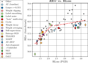
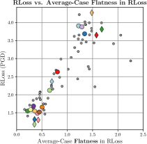
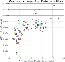
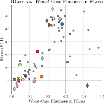
Figure 8: Robustness and Flatness: Left: RErr plotted against RLoss , showing that improved RLoss does not directly translate to reduced RErr for large RLoss . In these cases, reducing RLoss mainly means reducing the confidence of adversarial examples, which is necessary to improve adversarial robustness. Middle: RLoss or RErr (y-axis) plotted against our average-case flatness in RLoss . We highlight selected models, as in Tab. 1. Considering RLoss , we reveal a striking correlation between adversarial robustness and flatness. Popular AT variants improving robustness (e.g., TRADES, MART, etc.) also correspond to flatter minima. Vice versa, methods improving flatness (e.g., Entropy-SGD, weight decay, etc.) improve robustness obtained through AT. Subject to the non-trivial interplay between RErr and RLoss (cf. left), this relationship is also visible using RErr to quantify robustness. Right: RLoss (y-axis) plotted against worst-case flatness (x-axis) shows a less clear relationship. Still, improved flatness remains a necessity for better robust generalization, see Sec. 4.2 for discussion.

Our supplementary material includes additional details on the experimental setup and the evaluated methods. Furthermore, it contains an ablation regarding our average- and worst-case flatness measure and hyper-parameter ablation for individual methods, including training curves.

4.1 Understanding Robust Overfitting

In contrast to related work [103], we take a closer look at RLoss during robust overfitting because RErr is “blind” to many improvements in RLoss , especially on incorrectly classified examples. Fig. 5 shows training curves for various methods, i.e., RLoss /RErr over (normalized) epochs. For example, explicitly handling incorrectly classified examples during training, using MART, helps but does not prevent overfitting: RLoss for MART reduces compared to AT (first column). Unfortunately, this improvement does not translate to significantly better RErr , cf. Tab. 1. This discrepancy between RLoss and RErr can be reproduced for other methods, as well: label smoothing and label noise enforce, in expectation, the same target distribution. Thus, both reduce RLoss during overfitting (second column, top, rose and dark green). Label smoothing, however, does not improve RErr as significantly as label noise, i.e., does not prevent mis-classification. This illustrates an important aspect: against adversarial examples, “merely” improving RLoss does not translate to improved RErr if RLoss is high to begin with, i.e., “above” $-\ln(\nicefrac{{1}}{{K}}){\approx}2.3$ for $K{=}10$ classes. However, this is usually the case during robust overfitting. RErr , on the other hand, does not take into account the confidence of wrong predictions, i.e., it is “blind” for these improvements in RLoss . Label noise, in contrast, also improves RErr , which might be due to the additional randomness.

Similar to established methods, many “simple” regularization schemes prove surprisingly effective in tackling robust overfitting. For example, strong weight decay delays robust overfitting and AutoAugment prevents overfitting entirely, cf. Fig. 5 (third column). This indicates that popular AT variants, e.g., TRADES, AT with self-supervision or unlabeled examples, improve adversarial robustness by avoiding robust overfitting through regularization. This is achieved by preventing convergence on training examples (dotted). In regularization, however, hyper-parameters play a key role: even AT-AWP does not prevent robust overfitting if regularization is “too weak” (blue, fourth column). This is particularly prominent in terms of RLoss (top). Finally, learning rate schedules play an important role in how and when robust overfitting occurs (fifth column). However, as in [103], all schedules are subject to robust overfitting.

 

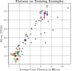
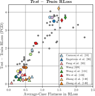
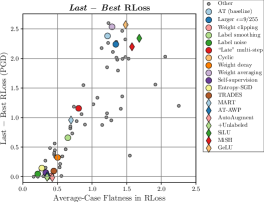
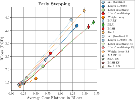
Figure 9: Robust Generalization and Early Stopping. Left: RLoss plotted vs. average-case flatness measured on training examples. Even on training examples, flatness is a good indicator for robust generalization. Middle: Robust generalization (RLoss ) decomposed into the test-train difference and the last-best (epoch) improvement (y-axis), both plotted against average-case flatness in RLoss (x-axis). In both cases, flatness seems to play an important role, i.e., flatness clearly reduces both the robust generalization gap and robust overfitting. Right: RLoss vs. average-case flatness in RLoss for selected models (all in supplementary material) with and without early stopping (“ES”). Early stopping consistently leads to improved adversarial robustness and better flatness.

4.2 Robust Generalization and Flatness in RLoss

As robust overfitting is primarily avoided through strong regularization, we hypothesize that this is because strong regularization finds flatter minima in the RLoss landscape. These flat minima help to improve robust generalization.

Flatness in RLoss “Explains” Overfitting: Using our average- and worst-case flatness measures in RLoss , we find that flatness reduces significantly during robust overfitting. Namely, flatness “explains” the increased RLoss caused by overfitting very well. Fig. 6 (left) plots RLoss , alongside average- and worst-case flatness and the maximum Hessian eigenvalue throughout training of our AT baseline. Clearly, flatness increases alongside (test) RLoss as soon as robust overfitting occurs. Note that the best epoch is $60$, meaning $0.4$ (black dotted). For further illustration, Fig. 6 (middle) explicitly plots RLoss (y-axis) against flatness in RLoss (x-axis) across epochs (dark blue to dark red): RLoss and flatness clearly worsen “alongside” each other during overfitting, for both average- and worst-case flatness. Methods such as AT with self-supervision, AT-AWP or AT with unlabeled examples avoid both robust overfitting and sharp minima (right). This relationship generalizes to different hyper-parameter choices of these methods: Fig. 7 plots RLoss (y-axis) vs. average-case flatness (x-axis) across different hyper-parameters. Again, e.g., for TRADES or AT-AWP, hyper-parameters with lower RLoss also correspond to flatter minima. In fact, Fig. 7 indicates that the connection between robustness and flatness also generalizes across different methods (and individual models).

Improved Robustness Through Flatness: Indeed, across all trained models, we found a strong correlation between robust generalization and flatness, using RLoss as measure for robust generalization. As discussed in Sec. 4.1, we mainly consider RLoss to assess robust generalization as improvements in RLoss above ${\sim}2.3$ have, on average, only small impact on RErr . Pushing RLoss below $2.3$, in contrast, directly translates to better RErr . This is illustrated in Fig. 8 (left) which plots RErr vs. RLoss for all evaluated models. To avoid this “kink” in the dotted red lines around $\text{RLoss}{\approx}2.3$, Fig. 8 (middle left) plots RLoss (y-axis) against average-case flatness in RLoss (x-axis), highlighting selected models. This reveals a clear correlation between robustness and flatness: More robust methods, e.g., AT with unlabeled examples or AT-AWP, correspond to flatter minima. Methods improving flatness, e.g., Entropy-SGD, weight decay or weight clipping, improve adversarial robustness. This also translates to RErr (middle right), subject to the described bend at $\text{RLoss}{\approx}2.3$. While many robust methods still obtain better flatness, activation functions such as SiLU, MiSH or GeLU also seem to improve flatness, without clear advantage in terms of robustness. Similarly, weight decay or clipping improve robustness considerably. Overall, with Pearson/Spearman correlation coefficients of $0.85$/$0.87$ ($p$-values ${<}10^{-21}$), we revealed a strong relationship between robustness and flatness.

Fig. 8 (right) shows that this relationship is less clear when considering worst-case flatness in RLoss (Pearson coefficient $0.54$). This is in contrast to [133] suggesting that worst-case flatness, in particular, is important to improve robustness of AT. However, worst-case flatness is more sensitive to $\xi$ and, thus, less comparable across methods. Note that worst-case robustness is still a good indicator for overfitting, cf. Fig. 6. All results are summarized in tabular form in Tab. 1: Grouping methods by good, average or poor robustness, we find that methods need at least “some” flatness, average- or worst-case, to be successful.

Decomposing Robust Generalization: So far, we used (absolute) RLoss on test examples as proxy of robust generalization. This is based on the assumption that deep models are generally able to obtain nearly zero train RLoss . However, this is not the case for many methods in Tab. 1 (second column). Thus, we also consider the robust generalization gap and the RLoss difference between last and best (early stopped) epoch. First, however, Fig. 9 (left) shows that flatness, when measured on training examples, is also a good predictor of (test) robustness. Then, Fig. 9 (middle left) explicitly plots the RLoss generalization gap (test$-$train RLoss , y-axis) against average-case flatness in RLoss (x-axis). Robust methods generally reduce this gap by both reducing test RLoss and avoiding convergence in train RLoss . Furthermore, Fig. 9 (middle right) considers the difference between last and best epoch, essentially quantifying the extent of robust overfitting. Again, methods with small difference, i.e., little robust overfitting, generally correspond to flatter minima. This is also confirmed in Fig. 9 (right) showing that early stopping essentially finds flatter minima along the training trajectory, thereby improving adversarial robustness. Altogether, flatness improves robust generalization by reducing both the robust generalization gap and the impact of robust overfitting.

More Results: Fig. 1 shows that the pre-trained models from RobustBench [24] confirm our observations so far (also see Fig. 9, middle left). While detailed analysis is not possible as only early stopped models are provided, they are consistently more robust and correspond to flatter minima compared to our models. This is despite using different architectures (commonly Wide ResNets [143]).

5 Conclusion

In this paper, we studied the relationship between adversarial robustness, specifically considering robust overfitting [103], and flatness of the robust loss (RLoss ) landscape w.r.t. perturbations in the weight space. We introduced both average- and worst-case measures for flatness in RLoss that are scale-invariant and allow comparison across models. Considering adversarial training (AT) and several popular variants, including TRADES [148], AT-AWP [133] or AT with additional unlabeled examples [16], we show a clear relationship between adversarial robustness and flatness in RLoss . More robust methods predominantly find flatter minima. Vice versa, approaches known to improve flatness, e.g., Entropy-SGD [17] or weight clipping [117] can help AT become more robust, as well. Moreover, even simple regularization methods such as AutoAugment [27], weight decay or label noise, are effective in increasing robustness by improving flatness. These observations also generalize to pre-trained models from RobustBench [24].

Appendix A Overview

In the main paper, we empirically studied the connection between adversarial robustness (in terms of the robust loss RLoss , i.e., the cross-entropy loss on adversarial examples) and flatness of the RLoss landscape w.r.t. changes in the weight space. In this context, we also consider the phenomenon of robust overfitting [103], i.e., that robustness on training examples increases consistently throughout training while robustness on test examples eventually decreases. Based on average- and worst-case metrics of flatness in RLoss , which we ensure to be scale-invariant, we show a clear relationship between adversarial robustness and flatness. This takes into account many popular variants of adversarial training (AT), i.e., training on adversarial examples: TRADES [148], MART [128], AT-AWP [133] AT with self-supervision [50] or additional unlabeled examples [16]. All of them improve adversarial robustness and flatness. Vice versa, approaches known to improve flatness, e.g., Entropy-SGD [17], weight clipping [117] or weight averaging [42] also improve adversarial robustness. Finally, we found that even simple regularization schemes, e.g., AutoAugment [27], weight decay or label noise, also improve robustness by finding flatter minima.

A.1 Contents

This supplementary material is organized as follows:

• Sec. B: additional discussion of related work.

• Sec. C: details on RLoss landscape visualization and comparison to [73] (cf. Fig. 10 and 11).

• Sec. D: details on how to compute our average- and worst-case flatness measures, including ablation studies in Sec. D.1 (cf. Fig. 12, 13 and 14).

• Sec. E: discussion of scale-invariance of our visualization and flatness measures (cf. Fig. 15 and Tab. 2).

• Sec. F: specifics on our experimental setup (training and evaluation details).

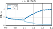
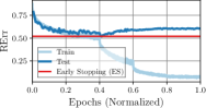
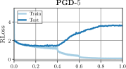
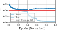
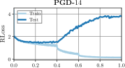
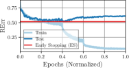
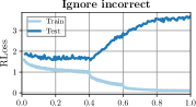
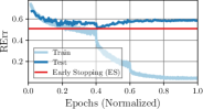
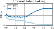
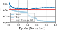
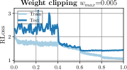
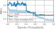
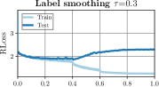
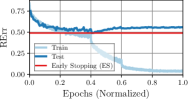
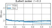
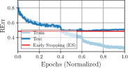
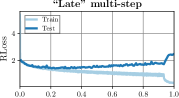
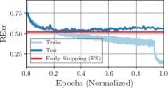
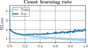
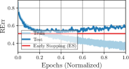
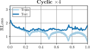
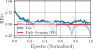
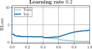
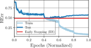
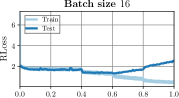
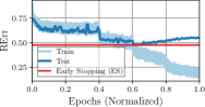
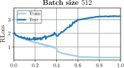
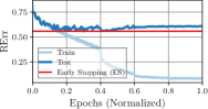
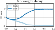
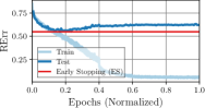
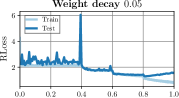
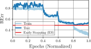
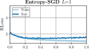
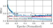
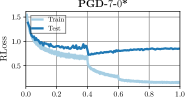
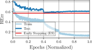
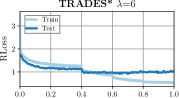
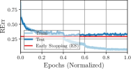
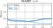
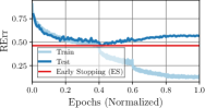
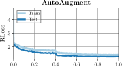
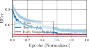
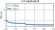
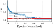
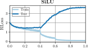
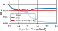
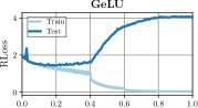
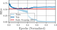
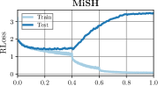
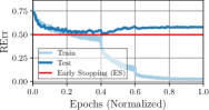
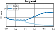
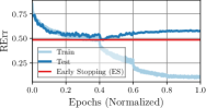
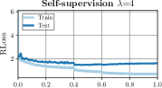
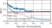
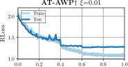
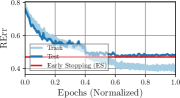
Figure 20: Training Curves: Test and train RLoss (top) and RErr (bottom), including RErr for early stopping, for all considered methods with selected hyper-parameters. * Train and test RLoss correspond to the attacks used during training, e.g., PGD-$\tau$ or maximizing KL-divergence for TRADES. $\dagger$ Reported RLoss corresponds to RLoss on adversarial examples without adversarial weights.

• Sec. G: discussion of all individual methods, including ablation regarding hyper-parameters in Sec. G.1 (cf. Fig. 16 and 17) and flatness in Sec. G.2 (cf. Fig. 18 and 19). Training curves for all methods in Fig. 20.

• Sec. H: all results in tabular form (Tab. 3, 4, 6, 5)

Appendix B Related Work

Adversarial Examples and Defenses: Adversarial examples, first reported in [122], can be generated using a wide-range of white-box attacks [122, 40, 67, 94, 87, 80, 14, 32, 78], with full access to the network, or black-box attacks [18, 11, 120, 54, 107, 88], with limited access to model queries. Besides certified and provable defenses [22, 138, 66, 147, 146, 130, 41, 39, 84, 113, 72, 23], adversarial training (AT) has become the de-facto standard, as discussed in the main paper. However, there are also many detection/rejection approaches [44, 38, 74, 79, 3, 83], so-called manifold-projection methods [55, 96, 109, 110], several methods based on pre-processing, quantization and/or dimensionality reduction [12, 98, 8], methods based on randomness, regularization or adapted architectures [144, 8, 89, 112, 48, 58, 104, 61, 70, 136] or ensemble methods [76, 116, 46, 126], to name a few directions. However, often these defenses can be broken by considering adaptive attacks [13, 15, 5, 6].

Weight Robustness: Flatness, w.r.t. the clean or robust loss surface, is also related to robustness in the weights. However, only few works explicitly study this “weight robustness”: [129] considers robustness w.r.t. $L_{\infty}$ weight perturbations, while [19] studies Gaussian noise on weights. [102, 47], in contrast, adversarially flip bits in (quantized) weights to reduce performance. Recently, [117] shows that robustness in weights can improve energy efficiency of neural network accelerators (i.e., specialized hardware for inference). This type of weight robustness is also relevant for some backdooring attacks that explicitly manipulate weights [59, 34]. Fault tolerance is also a related concept, as it often involved changes in units or weights. It has been studied in early works [90, 20, 28], obtaining fault tolerance using approaches similar to adversarial training NNs using approaches similar to adversarial training. However, there are also more recent works, e.g., weight dropping regularization [101] or GAN-based training [33]. We refer to [124] for a comprehensive survey.

Appendix C Visualization Details and Discussion

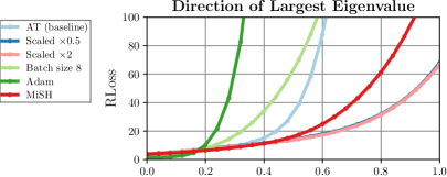
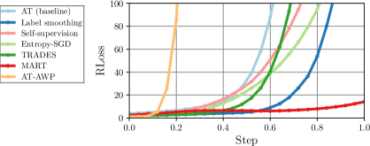
Figure 10: Visualization in “Hessian” Direction: RLoss visualized in the direction of the largest Hessian eigenvalue (i.e., the corresponding eigenvector). The eigenvalues quantify the “rate of change” along the corresponding eigenvector. Thus, the largest eigenvalue represents a worst-case direction in weight space. Clearly, RLoss increases significantly in these directions.

Visualization Details: For the plots in the main paper, we compute the mean RLoss across $10$ random, normalized directions; for adversarial directions, we plot max RLoss over $10$ adversarial directions. After normalization, we re-scale the weight directions to have length $0.5$ for random directions and $0.025$ for adversarial directions. This essentially “zooms in” and is particularly important when visualizing along adversarial weight directions. In all cases, we estimate RLoss on one batch of $128$ test examples for $51$ evenly spaced step sizes in $[-1,1]$. We found that using more test examples does not change the RLoss landscape significantly. Fig. 10 shows additional visualizations along the direction of the largest Hessian eigenvalue (also using per-layer normalization, multiplied by $0.5$).

Discussion of [73]: Originally, [73] uses a per-filter normalization instead of our per-layer normalization. Specifically, this means

$$\hat{\nu}^{(l,i)} =\frac{\nu^{(l)}}{\|\nu^{(l,i)}\|_{2}}\|w^{(l,i)}\|_{2}\quad\text{ for layer }l\text{, filter }i,$$ (6)

instead of our normalization outlined in the main paper:

$$\hat{\nu}^{(i)} =\frac{\nu^{(l)}}{\|\nu^{(l)}\|_{2}}\|w^{(l)}\|_{2}\quad\text{ for layer }l.$$ (7)

Furthermore, [73] does not consider changes in the biases or batch normalization parameters. Instead, we also normalize the biases as above and take them into account for visualization (but not the batch normalization parameters). More importantly, [73] considers only (clean) Loss , while we focus on RLoss . Compared to the plots from the main paper, Fig. 11 shows that the difference between filter-wise and layer-wise normalization has little impact in visually judging flatness. Generally, filter-wise normalization makes the RLoss landscape “look” flatter. However, this is mainly because the absolute step size, i.e., $\|\hat{\nu}\|_{2}$, is smaller compared to layer-wise normalization: for our AT baseline, this is (on average) $\|\hat{\nu}\|_{2}\approx 33.13$ for layer-wise and $\|\hat{\nu}\|_{2}\approx 21.49$ for filter-wise normalization.

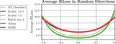
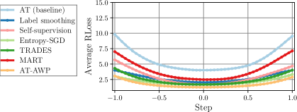
Figure 11: Filter-Wise Normalization: Compared to the RLoss landscape visualizations in the main paper, using per-layer normalization in Eq. (7), we follow [73] and use filter-wise normalization in Eq. (6). Again, we plot mean RLoss across $10$ random directions. However, this does not change results significantly, flatness remains difficult to judge and compare in an objective way. Filter-wise normalization, however, “looks” generally flatter.

Appendix D Computing Flatness in RLoss

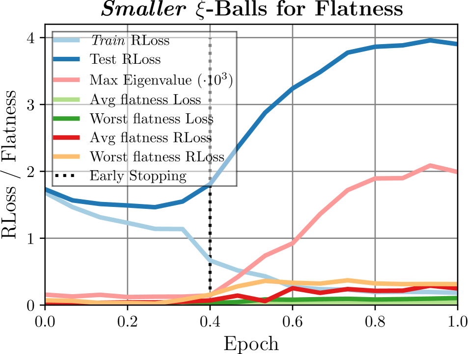
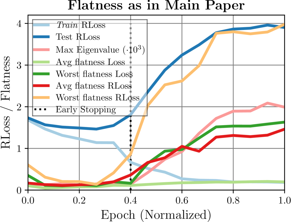
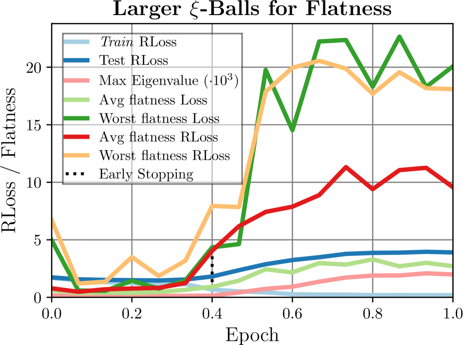
Figure 12: Flatness Throughout Training, Ablation: We plot train and test RLoss , maximum Hessian eigenvalue $\lambda_{\text{max}}$, average-/worst-case flatness of (clean) Loss as well as average-/worst-case flatness on RLoss . We consider $\xi{=}0.25$/$\xi{=}0.001$ (left), $\xi{=}0.5$/$\xi{=}0.003$ (middle and main paper), and $\xi{=}0.75$/$\xi{=}0.005$ for average-/worst-case flatness, respectively. If the neighborhood $b_{\xi}(w)$ is chosen too small (left), increases/changes in flatness during robust overfitting are difficult to measure due to fluctuations throughout training. Chosen too large (right), in contrast, worst-case flatness (both in Loss and RLoss ) quickly reaches unreasonably high loss values. This becomes problematic when comparing across models.

Average-Case Flatness: The average-case flatness measure in RLoss is defined as:

$$\begin{split}\mathbb{E}_{\nu}[\mathop{\rm max}\nolimits\limits_{\|\delta\|_{\infty}\leq\epsilon}\mathcal{L}(f(x{+}\delta,w{+}\nu),y)]\text{\hphantom{aaaaaaa}}\\ \text{\hphantom{aaaaaaa}}-\mathop{\rm max}\nolimits\limits_{\|\delta\|_{\infty}\leq\epsilon}\mathcal{L}(f(x{+}\delta;w),y)\end{split}$$ (8)

where $\mathbb{E}_{\nu}$ denotes the expectation over random weight perturbations $\nu\in B_{\xi}(w)$, $\mathcal{L}$ is the cross-entropy loss and $\mathop{\rm max}\nolimits_{\|\delta\|_{\infty}\leq\epsilon}\mathcal{L}(f(x{+}\delta;w),y)$ represents the robust loss (RLoss ). The first term is computed by randomly sampling $10$ weight perturbations from

$$B_{\xi}(w)=\{w+\nu:\|\nu^{(l)}\|_{2}\leq\xi\|w^{(l)}\|_{2}\forall\text{ layers }l\}.$$ (9)

For each weight perturbation $\nu$, the robust loss, defined as $\mathop{\rm max}\nolimits_{\|\delta\|_{\infty}\leq\epsilon}\mathcal{L}(f(x{+}\delta,w{+}\nu),y)$, is estimated using PGD with $20$ iterations ($\epsilon=\nicefrac{{8}}{{255}}$, learning rate $0.007$ and signed gradient). This is done per-batch (of size $128$) for the first $1000$ test examples. Alternatively, the weights perturbations $\nu$ could also be fixed across batches (i.e., $10$ samples in total for $\lceil\nicefrac{{1000}}{{128}}\rceil$ batches). However, this is not possible for our worst-case flatness measure, as discussed next. Thus, for comparability, we sample random weight perturbations for each batch individually. The second term is computed using PGD-$20$ with $10$ restarts, choosing the worst-case adversarial examples per test example (i.e., maximizing RLoss ).

Sampling in $B_{\xi}(w)$ is accomplished by sampling individually per layer. That is, for each layer $l$, we compute $\xi^{\prime}:=\xi\cdot\|w^{(l)}\|_{2}$ given the original weights $w$. Then, a random vector $\nu^{(l)}$ with $\|\nu^{(l)}\|_{2}\leq\xi^{\prime}$ is sampled. This is done for each layer, handling weights and biases as separate layers, but ignoring batch normalization [56] parameters.

Worst-Case Flatness: Worst-case flatness is defined as:

$$\begin{split}\mathop{\rm max}\nolimits_{\nu\in B_{\xi}(w)}\mathop{\rm max}\nolimits\limits_{\|\delta\|_{\infty}\leq\epsilon}&\mathcal{L}(f(x{+}\delta,w{+}\nu),y)\\ &-\mathop{\rm max}\nolimits\limits_{\|\delta\|_{\infty}\leq\epsilon}\mathcal{L}(f(x{+}\delta;w),y).\end{split}$$ (10)

Here, the expectation over $\nu$ in Eq. (8) is replaced by a maximum over $\nu\in B_{\xi}(w)$, considering smaller $\xi$. In practice, the first term in Eq. (10) is computed by jointly optimizing over weight perturbation $\nu$ and input perturbation(s) $\delta$ on a per-batch basis (of size $B=128$). This means, after random initialization of $\delta_{b}$, $\forall b=1,\ldots,B$, and $\nu\in B_{\xi}(w)$, each iteration computes and applies updates

$$\Delta_{\nu}=\nabla_{\nu}\sum_{b=1}^{B}\mathcal{L}(f(x_{b}+\delta_{b};w+\nu),y_{b})$$ (11)

$$\Delta_{\delta_{b}}=\nabla_{\delta_{b}}\sum_{b=1}^{B}\mathcal{L}(f(x_{b}+\delta_{b};w+\nu),y_{b})$$ (12)

before projecting $\delta_{b}$ and $\nu$ onto the constraints $\|\delta_{b}\|_{\infty}\leq\epsilon$ and $\|\nu^{(l)}\|_{2}\leq\xi\|w^{(l)}|_{2}$. The latter projection is applied in a per-layer basis, similar to sampling as described above. For the adversarial weight perturbation $\nu$, we use learning rate $0.001$, after normalizing the update $\Delta_{\nu}$ per-layer as in Eq. (7). We run $20$ iterations with $10$ restarts for each batch.

Flatness of Clean Loss Landscape: We can also consider both Eq. (8) and Eq. (10) on the clean (cross-entropy) loss (“Loss ”), i.e., $\mathcal{L}(f(x,w{+}\nu),y)$ instead of $\mathop{\rm max}\nolimits_{\|\delta\|_{\infty}\leq\epsilon}\mathcal{L}(f(x{+}\delta,w{+}\nu),y)$. We note that RLoss is an upper bound of (clean) Loss . Thus, flatness in RLoss and Loss are connected. However, Pearson correlation between RLoss and average-case flatness in (clean) Loss is only $0.27$, compared to $0.85$ for average-case flatness in RLoss . This indicates that correctly measuring flatness in RLoss is crucial to empirically establish a relationship between robustness and flatness.

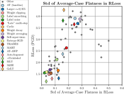
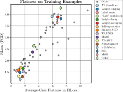
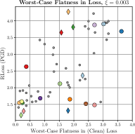
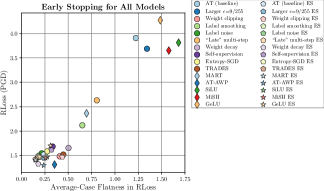
Figure 13: Left: Standard Deviation of Average-Case Flatness: We plot RLoss (y-axis) against the standard deviation (std) in our average-case flatness measure (x-axis). Note that the standard-deviation is due to the random weight perturbations $\nu$ in Eq. (8). Interestingly, more robust methods are not only flatter, but our average-case flatness measure also has lower standard deviation. Middle Left: Average-Case Flatness of Train RLoss : Test RLoss plotted against our average-case flatness measure as computed on training examples. Even on the training set, flatness is predictive of robust generalization, i.e., adversarial robustness on the test set. The relationship, however, is weaker compared to average-case flatness on test examples. Middle Right: Worst-Case Flatness in (Clean) Loss : As worst-case flatness in the clean Loss landscape also mirrors robust overfitting in Fig. 12, we plot RLoss against worst-case flatness in Loss . Even though flatness is measured considering clean Loss , many methods improving robustness (i.e., lower RLoss ) exhibit surprisingly good flatness. Right: Early Stopping for all Models: RLoss vs. average-case flatness for all models where early stopping improves adversarial robustness. For example, this is not the case for AutoAugment or AT with unlabeled examples. Across all models, early stopping improves both robustness and flatness. For clarity we provide a zoomed-in plot for the lower left corner.

D.1 Ablation for Flatness Measures

Flatness Throughout Training: Fig. 12 shows average- and worst-case flatness on both clean as well as robust loss (Loss and RLoss ) throughout training of our AT baseline. We consider different sizes of the neighborhood $B_{\xi}(w)$ for computing our flatness measures: $\xi{=}0.25$/$\xi{=}0.001$ (left), $\xi{=}0.5$/$\xi{=}0.003$ (middle, as in main paper), and $\xi{=}0.75$/$\xi{=}0.005$ for average-/worst-case flatness, respectively. While average-case flatness of clean Loss does not mirror robust overfitting very well, its worst-case pendant increases during overfitting, even though RLoss is not taken into account. Furthermore, if the neighborhood $B_{\xi}(w)$ is chosen too small, the flatness measures are not sensitive enough to be discriminative (cf. left). Fig. 12 also shows that, throughout training of one model, the largest Hessian eigenvalue mirrors robust overfitting. Overall, this means that early stopping essentially improves adversarial robustness by finding flatter minima. This is confirmed in Fig. 13 (right), showing that early stopping consistently improves robustness and flatness.

Standard Deviation in Average-Case Flatness: In Fig. 13 (left), the x-axis plots the standard deviation in our average-case flatness measure (in RLoss ). Note that the standard deviation originates in the random samples $\nu$ used to calculate Eq. (8). First of all, standard deviation tends to be small (i.e., $\leq 0.3$) across almost all models. This means that our findings in the main paper, i.e., the strong correlation between flatness and RLoss , is supported by low standard deviation. More importantly, the standard deviation reduces for particularly robust methods.

Average-Case Flatness on Training Examples: Fig. 13 (middle left) shows that average-case flatness in RLoss is also predictive for robust generalization when computed on training examples. However, the correlation between (test) RLoss and (train) flatness is less clear, i.e., there is a larger “spread” across methods. Here, we use the first $1000$ training examples to compute average-case flatness.

Worst-Case Flatness on Clean Loss : In Fig. 12, worst-case flatness on clean Loss also correlates with robust overfitting. Thus, in Fig. 13 (middle right), we plot RLoss against worst-case flatness of Loss , showing that there is no clear relationship across models. Nevertheless, many methods improving adversarial robustness also result in flatter minima in the clean loss landscape. This is sensible as RLoss is generally an upper bound for (clean) Loss . On the other hand, flatness in Loss is not discriminative enough to clearly distinguish between robust and less robust models.

 

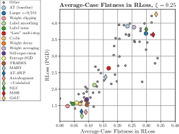
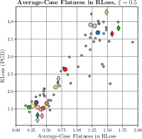
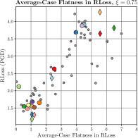
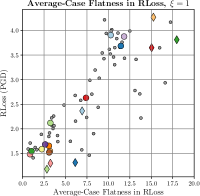
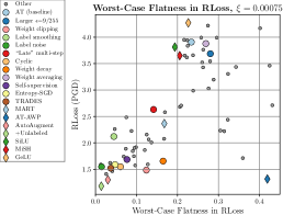
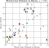
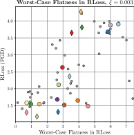
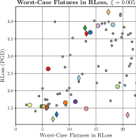
Figure 14: Flatness in RLoss , Ablation for $B_{\xi}(w)$: RLoss (y-axis) plotted against average-case (top) and worst-case (bottom) flatness in RLoss (x-axis). Top: We consider $\xi\in\{0.25,0.5,0.75,1\}$ for average-case flatness. The clear relationship between adversarial robustness, i.e., low RLoss , and flatness shown for $\xi=0.5$ in the main paper can be reproduced for all cases. Bottom: For worst-case flatness, we consider $\xi\in\{0.00075,0.001,0.003,0.005\}$. When chosen too large, e.g., $\xi=0.005$, however, variance seems to increase, making the relationship less clear. For small $\xi$, e.g., $\xi=0.00075$, the correlation between robustness and flatness is pronounced, except for a few outliers, including AT-AWP [133].

Ablation for $B_{\xi}(w)$: For computing our average- and worst-case flatness measures (in RLoss ), we considered various sizes of neighborhoods in weight space, i.e. $B_{\xi}(w)$ from Eq. (9) for different $\xi$. Fig. 14 considers $\xi\in\{0.25,0.5,0.75,1\}$ for average-case flatness (top) and $\xi\in\{0.00075,0.001,0.003,0.005\}$ for worst-case flatness (bottom). In both cases, we plot RLoss (y-axis) against flatness in RLoss (y-axis), as known from the main paper. Average-case flatness using small $\xi=0.25$ results in significantly smaller values, between $0$ and $0.4$, i.e., the increase in RLoss in random weight directions is rather small. Still, the relationship between adversarial robustness and flatness is clearly visible. The same holds for larger $\xi\in\{0.75,1\}$. Worst-case flatness generally gives a less clear picture regarding the relationship between robustness and flatness. Additionally, for larger $\xi\in\{0.003,0.005\}$, variance seems to increase such that this relationship becomes less pronounced. In contrast to average-case flatness, the variance is not induced by the $10$ restarts used for Eq. (10), but caused by training itself. Indeed, re-training our AT baseline leads to a worst-case flatness in RLoss of $5.1$, a significant reduction from $6.49$ as obtained for our original baseline. Overall, however, the observations from the main paper can be confirmed using different sizes of the neighborhood $B_{\xi}(w)$.

Appendix E Scaling Networks and Scale-Invariance

Scale-Invariance: In the main paper, we presented a simple experiment to show that our measures of flatness in RLoss are scale-invariant: we scaled weights and biases of all convolutional layers in our adversarially trained ResNet-18 [45] by factor $s\in\{0.5,2\}$. Note that all convolutional layers in the ResNet are followed by batch normalization layers [56]. Thus, the effect of scaling is essentially “canceled out”, i.e., these convolutional layers are scale-invariant. Thus, the prediction stays roughly constant. Fig. 15 (left) shows RLoss landscape visualizations for AT and its scaled variants in random and adversarial weight directions. Clearly, scaling AT has negligible impact on the RLoss landscape in both cases. Fig. 15 (right) shows that our flatness measures remain invariant, as well. As $B_{\xi}(w)$ in Eq. (9) is defined per-layer (weights and biases separately) and relative to $w$, the neighborhood increases alongside the weights, rendering visualization and flatness measures invariant. When, for example, scaling up specific layers and scaling down others, as discussed in [31], causes the neighborhood $B_{\xi}(w)$ to increase or decrease in size for these particular layers. Thus, following [31], scaling up the first layer of a two-layer ReLU network by $\alpha$ and scaling down the second layer by $\nicefrac{{1}}{{\alpha}}$ (keeping the output constant), has no effect in terms of measuring flatness as the per-layer neighborhood $B_{\xi}(w)$ is scaled accordingly, as well. The Hessian eigenspectrum, in contrast, scales with the models, cf. Tab. 2, and is not suited to quantify flatness.

Convexity and Flatness: Tab. 2 also presents the convexity metric introduced in [73]: $\nicefrac{{|\lambda_{\text{min}}|}}{{|\lambda_{\text{max}}|}}$ with $\lambda_{\text{min/max}}$ being largest/smallest Hessian eigenvalue. Note that the Hessian is computed following [73] w.r.t. to the clean (cross-entropy) loss, not taking into account adversarial examples. The intuition is that negative eigenvalues with large absolute value correspond to non-convex directions in weight space. If these eigenvalues are large in relation to the positive eigenvalues, there is assumed to be significant non-convexity “around” the found minimum. Tab. 2 shows that this fraction is usually very small, as also found in [73]. However, Tab. 2 also shows that this convexity measure is not clearly correlated with adversarial robustness.

Appendix F Detailed Experimental Setup

We focus our experiments on CIFAR10 [65], consisting of $50\text{k}$ training examples and $10\text{k}$ test examples of size $32\times 32$ (in color) and $K=10$ class labels. We use all training examples during training, but withhold the last $500$ test examples for early stopping. Evaluation is performed on the first $1000$ test examples, due to long runtimes of AutoAttack [26] and our flatness measures (on RLoss ). Any evaluation on the training set is performed on the first $1000$ training examples (e.g., in Fig. 13, middle).

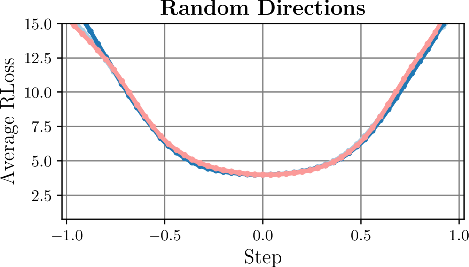
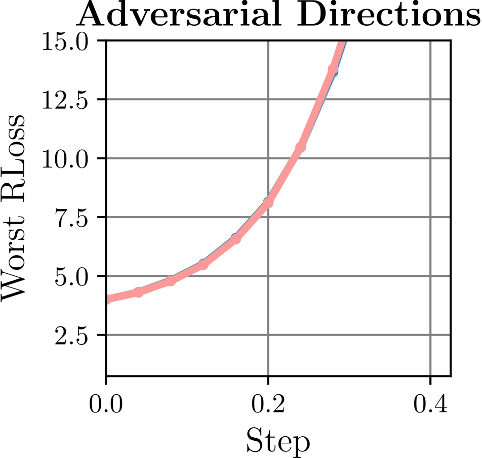
Model	Robustness		Flatness
	RErr $\downarrow$	RErr $\downarrow$	Worst	Avg	Worst
	(test)	(train)	Loss	RLoss	RLoss
Scaled $\times 0.5$	60.9	8.4 (-52.5)	0.86	1.36	6.50
AT (baseline)	61.0	8.4 (-52.6)	0.86	1.21	6.48
Scaled $\times 2$	61.0	8.3 (-52.7)	0.86	1.27	6.49

Figure 15: Flatness and Scale-Invariance. Left: We plot average RLoss and worst RLoss along random and adversarial directions, as discussed in Sec. C, for AT and its scaled variants, $\times 0.5$ and $\times 2$. Clearly, RLoss landscape looks nearly identical. Right: Robustness against PGD-$20$ on train and test examples, as well as average- and worst-case flatness measures on RLoss . For completeness, we also include worst-case flatness on clean Loss . All of these measures are nearly invariant to scaling. The shown differences can be attributed to randomness in computing these measures.

As network architecture, we use ResNet-18 [45] with batch normalization [56] and ReLU activations. Our AT baseline (i.e., default model) is trained using SGD for $150$ epochs, batch size $128$, learning rate $0.05$, reduced by factor $0.1$ at $60$, $90$ and $120$ epochs, weight decay $0.005$ and momentum $0.9$. We save snapshots every $5$ epochs to perform early stopping, but do not use early stopping by default. We whiten input examples by subtracting the (per-channel) mean and dividing by standard deviation. We use standard data augmentation, considering random flips and cropping (by up to $4$ pixels per side). By default, we use $7$ iterations PGD, with learning rate $0.007$, signed gradient and $\epsilon=\nicefrac{{8}}{{255}}$ to compute $L_{\infty}$ adversarial examples. Note that no momentum [32] or backtracking [119] is used for PGD. The training curves in Fig. 20 correspond to robustness measured using the $7$-iterations PGD attack used for training, which we also use for early stopping (with $5$ random restarts).

For evaluation, we run PGD for $20$ iterations and $10$ random restarts, taking the worst-case adversarial example per test example [119]. Our results considering robust loss (RLoss ) are based on PGD, while we report robust test error (RErr ) using AutoAttack [26]. Note that AutoAttack does not maximize cross-entropy loss as it stops when adversarial examples are found. Thus, it is not suitable to estimate RLoss . Robust test error is calculated as the fraction of test examples that are either mis-classified or successfully attacked. The distinction between PGD-$20$ and AutoAttack is important as AutoAttack does not maximize cross-entropy loss, resulting in an under-estimation of RLoss , while PGD-$20$ generally underestimates RErr . Computation of our average- and worst-case flatness measure is detailed in Sec. D.

Everything is implemented in PyTorch [95].

Appendix G Methods

In the following, we briefly elaborate on the individual methods considered in our experiments.

Learning Rate Schedules: Besides our default, multi-step learning rate schedule (learning rate $0.05$, reduced by factor $0.1$ after epochs $60$, $90$, and $120$), we followed [92] and implemented the following learning rate schedules: First, simply using a constant learning rate of $0.05$. Second, only two “late” learning rate reductions at epochs $140$ and $145$, as done in [99]. Third, using a cyclic learning rate, interpolating between a learning rate of $0.2$ and $0$ for $30$ epochs per cycle, as, e.g., done in [132]. We consider training for up to $4$ cycles ($=120$ epochs). These learning rate schedules are available as part of PyTorch [95].

Label Smoothing: In [121], label smoothing is introduced as regularization to improve (clean) generalization by not enforcing one-hot labels in the cross-entropy loss. Instead, for label $y$ and $K=10$ classes, a target distribution $p\in[0,1]^{K}$ (subject to $\sum_{i}p_{i}=1$) with $p_{y}=1-\tau$ (correct label) and $p_{i}=\nicefrac{{\tau}}{{K-1}}$ for $i\neq y$ (all other labels) is enforced. During AT, we only apply label smoothing for the weight update, not for PGD. We consider $\tau\in\{0.1,0.2,0.3\}$.

Label Noise: Instead of explicitly enforcing a “smoothed” target distribution, we also consider injecting label noise during training. In each batch, we sample random labels for a fraction of $\tau$ of the examples. Note that the labels are sampled uniformly across all $K=10$ classes. Thus, in expectation, the enforced target distribution is $p_{y}=1-\tau+\nicefrac{{\tau}}{{K}}$ and $p_{i}=\nicefrac{{\tau-\nicefrac{{\tau}}{{K}}}}{{K-1}}$. As result, this is equivalent to label smoothing with $\tau=\tau-\nicefrac{{\tau}}{{K}}$. In contrast to label smoothing, this distribution is not enforced explicitly in the cross-entropy loss. As above, adversarial examples are computed against the true labels (without label noise) and label noise is injected for the weight update. We consider $\tau\in\{0.1,0.2,0.3,0.4,0.5\}$. While label smoothing does not further improve adversarial robustness for $\tau>0.3$, label noise proved very effective in avoiding robust overfitting, which is why we also consider $\tau=0.4$ or $0.5$.

Weight Averaging: To implement weight averaging [57], we follow [42] and keep a “running” average $\bar{w}$ of the model’s weights throughout training, updated in each iteration $t$ as follows:

$$\bar{w}^{(t)}=\tau\bar{w}^{(t-1)}+(1-\tau)w^{(t)}$$ (13)

where $w^{(t)}$ are the weights in iteration $t$ after the gradient update. Weight averaging is motivated by finding the weights $\bar{w}$ in the center of the found local minimum. As, depending on the learning rate, training tends to oscillate, the average of the iterates is assumed to be close to the actual center of the minimum. In our experiments, we consider $\tau\in\{0.98,0.985,0.99,0.9975\}$.

Weight Clipping: Following [117], we implement weight clipping by clipping the weights to $[-w_{\text{max}},w_{\text{max}}]$ after each training iteration. We found that $w_{\text{max}}$ can be chosen as small as $0.005$, which we found to work particularly well. Larger $w_{\text{max}}$ does not have significant impact on adversarial robustness for AT. [117] argues that weight clipping together with minimizing cross-entropy loss leads to more redundant weights, improving robustness to random weight perturbations. As result, we also expect weight clipping to improve flatness. We consider $w_{\text{max}}\in\{0.005,0.01,0.025\}$.

Ignoring Incorrect Examples & Preventing Label Leaking: As robust overfitting in AT leads to large RLoss on incorrectly classified test examples, we investigate whether (a) not computing adversarial examples on incorrectly classified examples (during training) or (b) computing adversarial examples against the predicted (not true) label (during training) helps to mitigate robust overfitting. These changes can be interpreted as ablations of MART [128] and are easily implemented. Note that option (b) is essentially computing adversarial examples without label leaking [68]. However, as shown in Fig. 16, these two variants of AT have little to no impact on robust overfitting.

Model (RErr against AutoAttack [25])	RErr $\downarrow$	$\lambda_{\text{max}}$	$\frac{|\lambda_{\text{min}}|}{|\lambda_{\text{max}}|}$
AT (baseline)	62.8	1990	0.088
Scaled $\times 0.5$	62.8	7936	0.088
Scaled $\times 2$	62.8	505	0.088
Batch size $8$	58.2	3132	0.027
Adam	57.5	540	0.047
Label smoothing	61.2	2484	0.085
Self-supervision	57.1	389	0.041
Entropy-SGD	58.6	5773	0.054
TRADES	56.7	947	0.089
MART	61	1285	0.087
AT-AWP	54.3	1200	0.241

Table 2: Hessian Eigenvalue $\lambda_{\text{max}}$ and Convexity: For the models from Fig. 10 and 11, we report RErr against AutoAttack [26], the maximum Hessian eigenvalue $\lambda_{\text{max}}$ and the convexity measure of [73] computed as $\nicefrac{{|\lambda_{\text{min}}|}}{{|\lambda_{\text{max}}|}}$. This fraction is supposed to quantify the degree of non-convexity around the found minimum. As can be seen, neither $\lambda_{\text{max}}$ nor convexity correlate well with adversarial robustness. Regarding $\lambda_{\text{max}}$ this is due to the Hessian eigenspectrum not being scale-invariant, as shown for scaled versions ($\times 0.5$ and $\times 2$) of our AT baseline.

AutoAugment: In [27], an automatic procedure for finding data augmentation policies is proposed, so-called AutoAugment. We use the found CIFAR10 policy (cf. [27], appendix), which includes quite extreme augmentations. For example, large translations are possible, rendering the image nearly completely uniform, only leaving few pixels at the border. In practice, AutoAugment usually prevents convergence and, thus, avoids overfitting. We further combine AutoAugment with CutOut [29] (using random $16\times 16$ “cutouts”). We apply both AutoAugment and CutOut on top of our standard data augmentation, i.e., random flipping and cropping. We use publicly available PyTorch implementations.

Entropy-SGD [17] explicitly encourages flatter minima by taking the so-called “local” entropy into account. As a result, Entropy-SGD not only finds “deep” minima (i.e., low loss values) but also flat ones. In practice, this is done using nested SGD: the inner loop approximates the local entropy using stochastic gradient Langevin dynamics (SGLD), the outer loop updates the weights. The number of inner iterations is denoted by $L$. While the original work [17] uses $L$ in $[5,20]$ on CIFAR10, we experiment with $L\in\{1,2,3,5\}$. Note that, for fair comparison, we train for $\nicefrac{{150}}{{L}}$ epochs. For details on the Entropy-SGD algorithm, we refer to [17]. Our implementation follows the official PyTorch implementation.

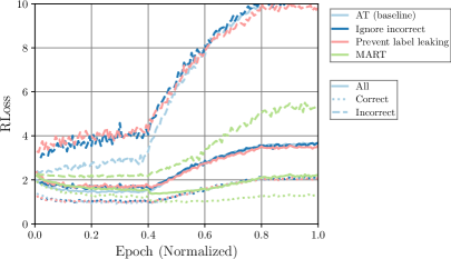
Figure 16: Approaches of Handling Incorrect Examples: We plot test RLoss on all (solid), correctly classified (dotted) and incorrectly classified (dashed) examples throughout training. We consider our AT baseline (light blue), ignoring incorrectly classified training examples in the RLoss computation during training (dark blue) and preventing label leaking by computing adversarial examples against the predicted labels during training (rose). However, these “simple” approaches of tackling the high RLoss on incorrectly classified test examples are not successful in reducing robust overfitting. As outlined in the main paper, MART [128] (green) is able to dampen overfitting through an additional robust KL-loss weighted by confidence, see text.

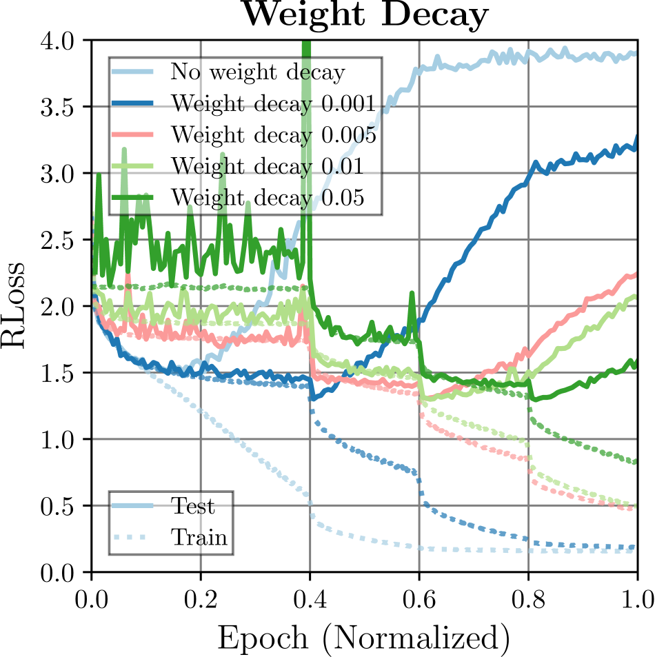
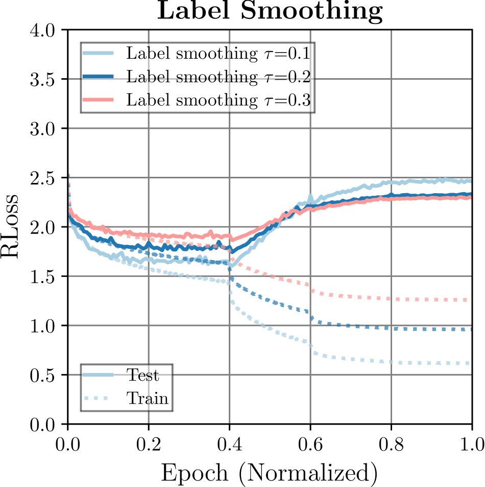
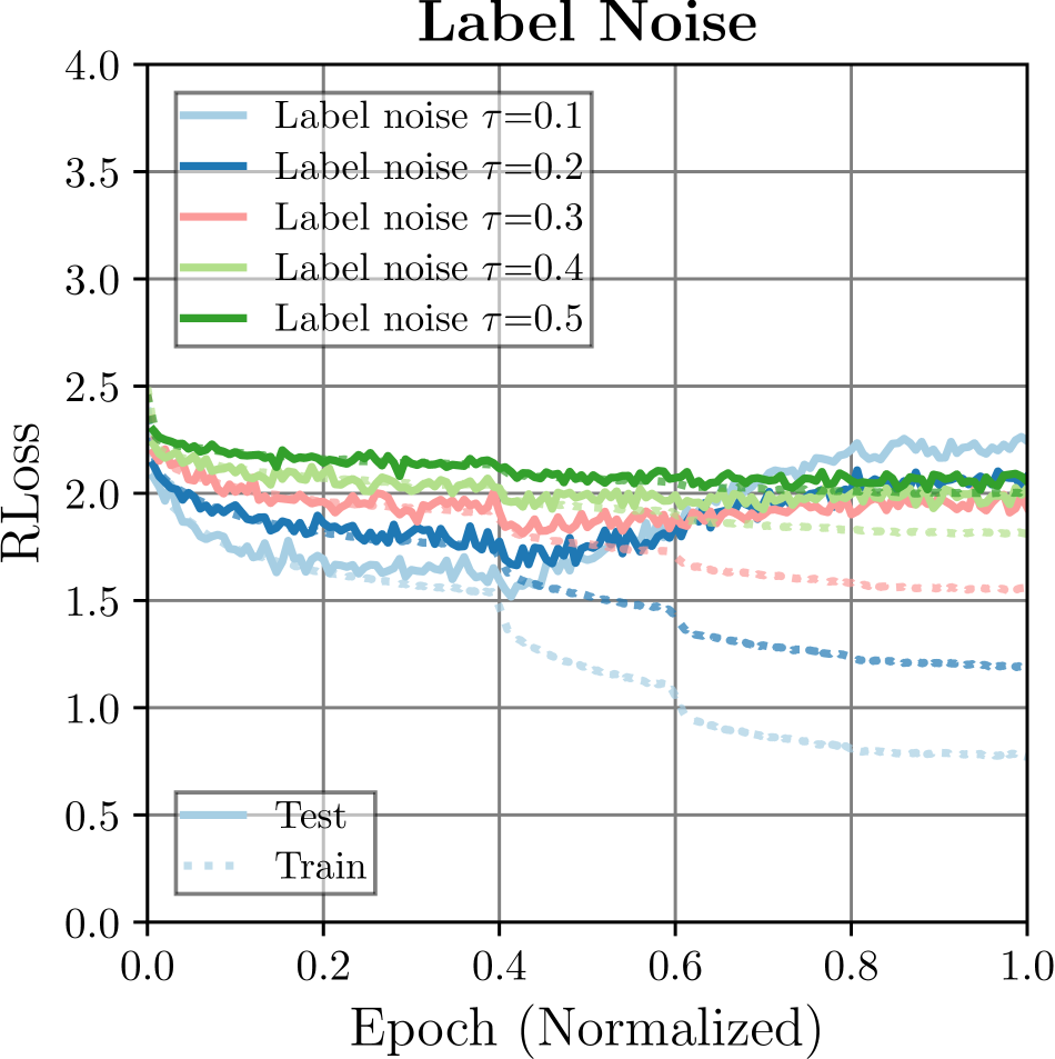
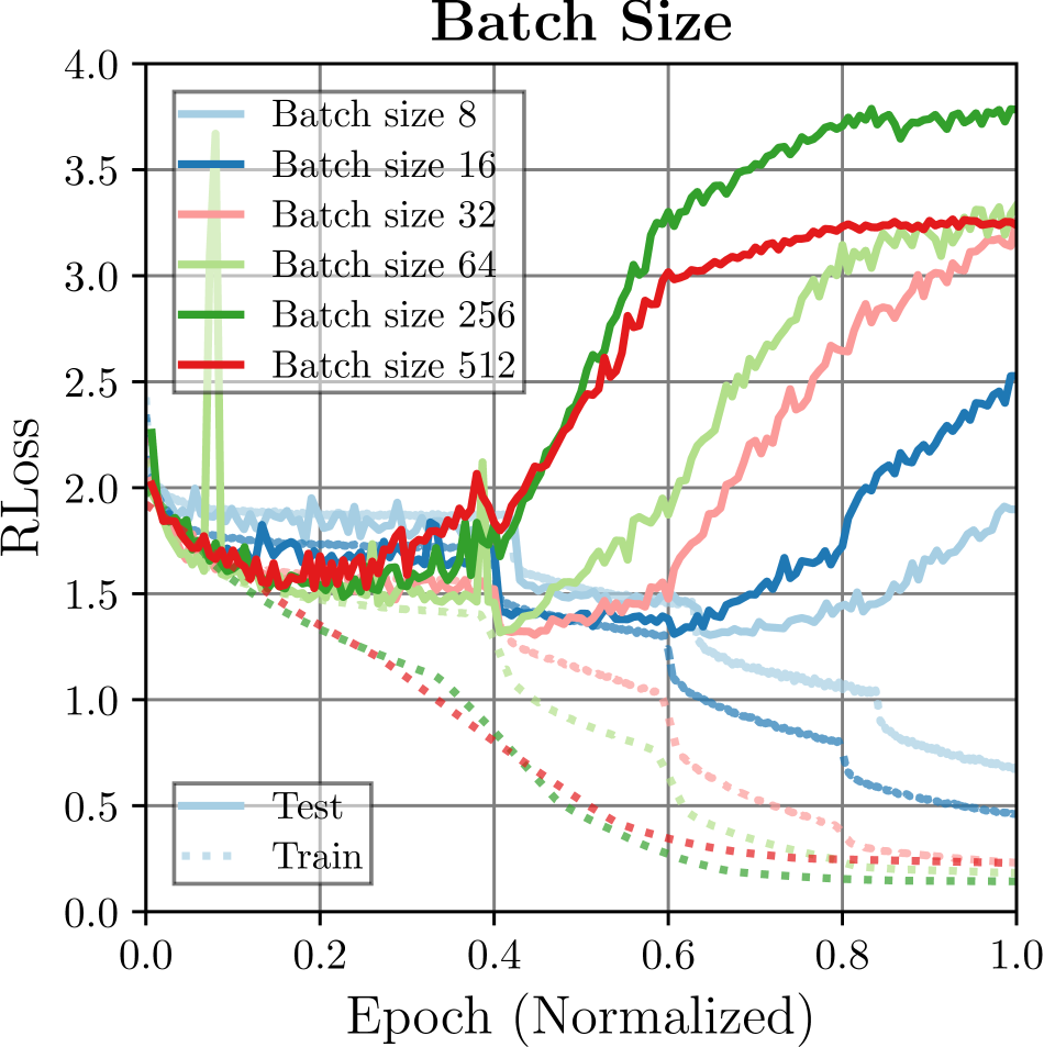
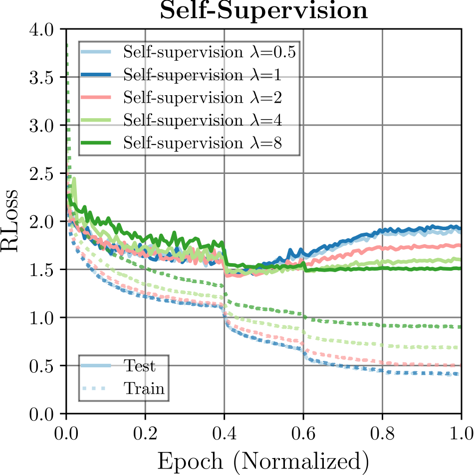
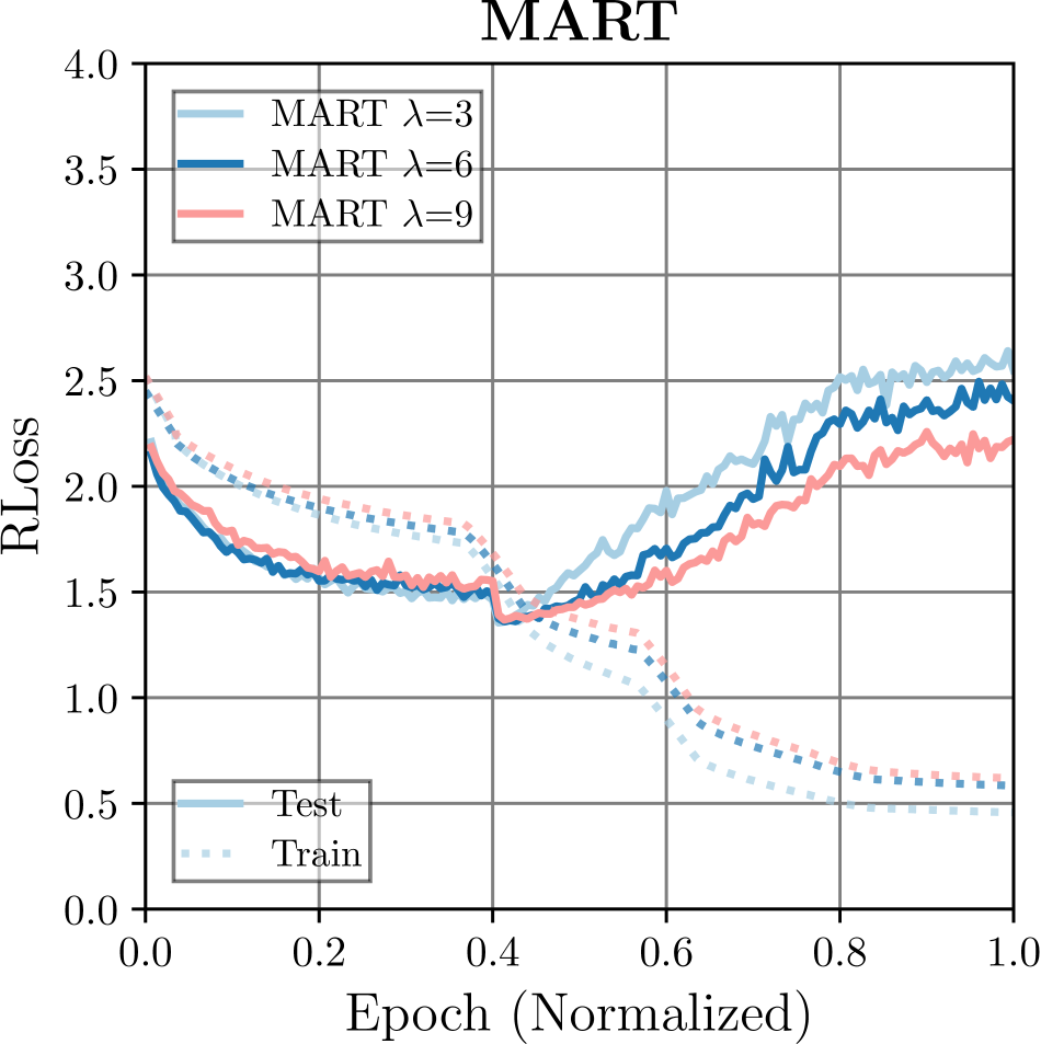
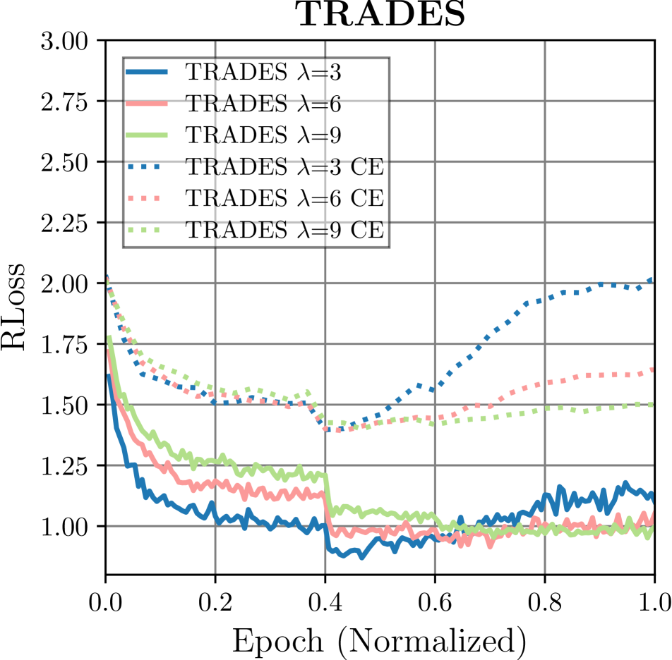
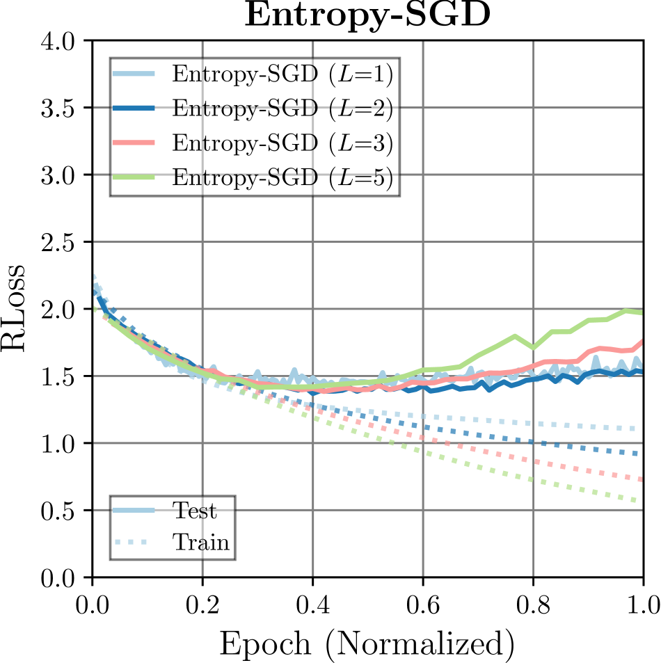
Figure 17: Training Curves for Varying Hyper-Parameters: We plot RLoss for selected methods and hyper-parameters to demonstrate the impact of hyper-parameters on avoiding or reducing robust overfitting. Note that, for TRADES, we show both RLoss on adversarial examples computed by maximizing the KL-divergence in Eq. (18) (solid) and on adversarial examples obtained by maximizing cross-entropy loss (“CE”, dotted).

Activation functions: We consider three recently proposed activation functions: SiLU [35], MiSH [85] and GeLU [49]. These are defined as:

$$(\text{SiLU})\quad x\sigma(x)\text{ with }\sigma(x)=\nicefrac{{1}}{{(1+\exp(-x))}},$$ (14)

$$(\text{MiSH})\quad x\tanh(\log(1+\exp(x))),$$ (15)

$$(\text{GeLU})\quad x\sigma(1.702x).$$ (16)

All of these activation functions can be seen as smooth versions of the ReLU activation. In [114], some of these activation functions are argued to avoid robust overfitting due to lower curvature compared to ReLU.

AT-AWP: AT with adversarial weight perturbations (AT-AWP) [133] computes adversarial weight perturbations on top of adversarial examples to further regularize training. This is similar to our worst-case flatness measure of RLoss , however, adversarial examples and adversarial weights are computed sequentially, not jointly, and only one iteration is used to compute adversarial weights. Specifically, after computing adversarial examples $\tilde{x}=x+\delta$, an adversarial weight perturbation $\nu$ is computed by solving

$$\mathop{\rm max}\nolimits_{\nu\in B_{\xi}(w)}\mathcal{L}(f(\tilde{x};w+\nu),y)$$ (17)

with $B_{\xi}(w)$ as in Eq. (9) using one iteration of gradient ascent with fixed step size of $\xi$. The gradient is normalized per layer as in Eq. (7). We considered $\xi\in\{0.0005,0.001,0.005,0.01,0.015,0.02\}$ and between $1$ and $7$ iterations and found that $\xi=0.01$ and $1$ iteration works best (similar to [133]).

TRADES: [148] proposes an alternative formulation of AT that allows a better trade-off between adversarial robustness and (clean) accuracy. The loss to be minimized is

$$\begin{split}\mathcal{L}&(f(x;w),y)\\ &+\lambda\mathop{\rm max}\nolimits_{\|\delta\|_{\infty}\leq\epsilon}\text{KL}(f(x;w),f(x+\delta;w)).\end{split}$$ (18)

During training, adversarial examples are computed by maximizing the KL-divergence (instead of cross-entropy loss), i.e., using the second term in Eq. (18). Commonly $\lambda=6$ is chosen, however, we additionally tried $\lambda\in\{1,3,6,9\}$. We follow the official implementation.

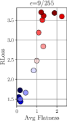
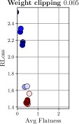
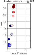
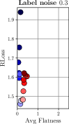
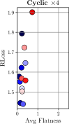
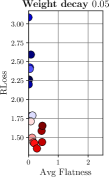
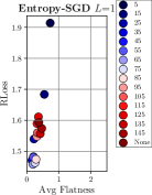
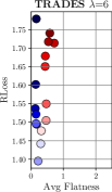
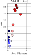
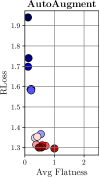
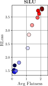
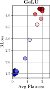
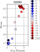
Figure 18: Flatness Throughout Training: Complementary to the main paper, we plot RLoss against average-case flatness in RLoss for selected methods throughout training epochs. Early epochs are shown in dark blue, late epochs are shown in dark red. For cyclic learning rate, we show $4$ cycles with a total of $120$ epochs. For many methods not avoiding robust overfitting, flatness decreases alongside an increase in RLoss during overfitting. Using, e.g., AutoAugment, label noise or Entropy-SGD, in contrast, both effects are reduced.

MART [128] explicitly addresses the problem of incorrectly classified examples during training. First, the cross-entropy loss $\mathcal{L}$ for training is replaced using a binary cross-entropy loss $\mathcal{L}_{\text{bin}}$, i.e., classifying correct class vs. most-confident “other” class:

$$\begin{split}\mathcal{L}_{\text{bin}}(f(x;w),y)=&-\log(f_{y}(x;w))\\ &-\log(1-\mathop{\rm max}\nolimits_{y^{\prime}\neq y}f_{y^{\prime}}(x;w)).\end{split}$$ (19)

Second, the KL-divergence used in TRADES in Eq. (18) is combined with a confidence-based weight:

$$\begin{split}\mathcal{L}_{\text{bin}}&(f(\tilde{x};w),y)\\ &+\lambda\text{KL}(f(x;w),f(\tilde{x};w)()(1-f_{y}(x;w))\end{split}$$ (20)

Adversarial examples are still computed by maximizing regular cross-entropy loss. We follow the official implementation. MART is successful in reducing robust overfitting on incorrectly classified examples, as shown in Fig. 16.

PGD-$\tau$: In [150], a variant of PGD is proposed for AT: PGD-$\tau$ stops maximization $\tau$ iterations after the label flipped. This is supposed to find “friendlier” adversarial examples that can be used for AT. Note that $\tau=0$ also does not compute adversarial examples on incorrectly classified training examples. We consider $\tau\in\{0,1,2,3\}$.

Self-Supervision: Following [50], we implement AT using rotation-prediction as additional self-supervised task. Note, however, that no additional (unlabeled) training examples are used. Specifically, the following learning problem is tackled:

$$\begin{split}\mathop{\rm max}\nolimits&{}_{\|\delta\|_{\infty}\leq\epsilon}\mathcal{L}(f(x+\delta;w),y)\\ &+\lambda\mathop{\rm max}\nolimits_{\|\delta\|_{\infty}\leq\epsilon}\mathcal{L}(f(\text{rot}(x+\delta,r);w),y_{r})\\ &r\in\{0,90,180,270\},y_{r}\in\{0,1,2,3\}\end{split}$$ (21)

where $\text{rot}(x,r)$ rotates the training example $x$ by $r$ degrees. In practice, we split every batch in half: The first half uses the original training examples with correct labels. Examples in the second half are rotated randomly by $\{0,90,180,270\}$ degrees, and the labels correspond to the rotation (i.e., $\{0,1,2,3\}$). Adversarial examples are computed against the true or rotation-based labels. Note that, in contrast to common practice [115], we do not predict all four possible rotations every batch, but just one randomly drawn per example. We still use $150$ epochs in total. We consider $\lambda\in\{0.5,1,2,4,8\}$.

Additional Unlabeled Examples: As proposed in [16, 2], we also consider additional, pseudo-labeled examples during training. We use the provided pseudo-labeled data from [16] and split each batch in half: using $50\%$ original CIFAR10 training examples, and $50\%$ pseudo-labeled training examples from [16]. We still use $150$ epochs in total. We follow the official PyTorch implementation.

G.1 Training Curves

Fig. 17 shows (test) RLoss throughout training for selected methods and hyper-parameters. Across all methods, we found that hyper-parameters have a large impact on robust overfitting. For example, weight decay or smaller batch sizes can reduce and delay robust overfitting considerably if regularization is “strong” enough, i.e., large weight decay or low batch size (to induce more randomness). For the other methods, difference between hyper-parameters is more subtle. However, across all cases, reduced overfitting generally goes hand in hand with higher RLoss on training examples, i.e., the robust generalization gap is reduced. This indicates that avoiding convergence on training examples plays an important role in avoiding robust overfitting.

Training curves for all methods are shown in Fig. 20.

G.2 Flatness for Methods

 

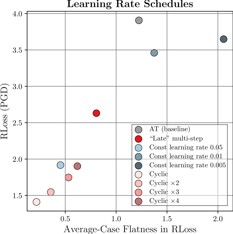
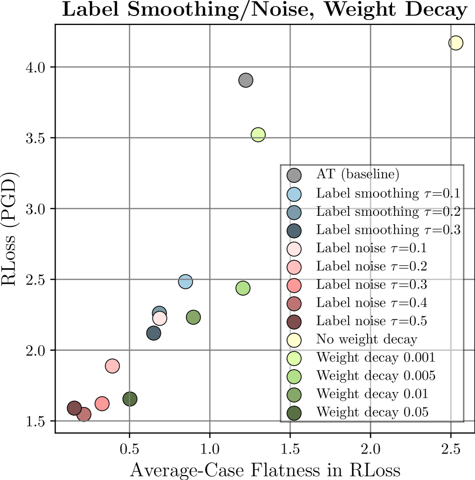
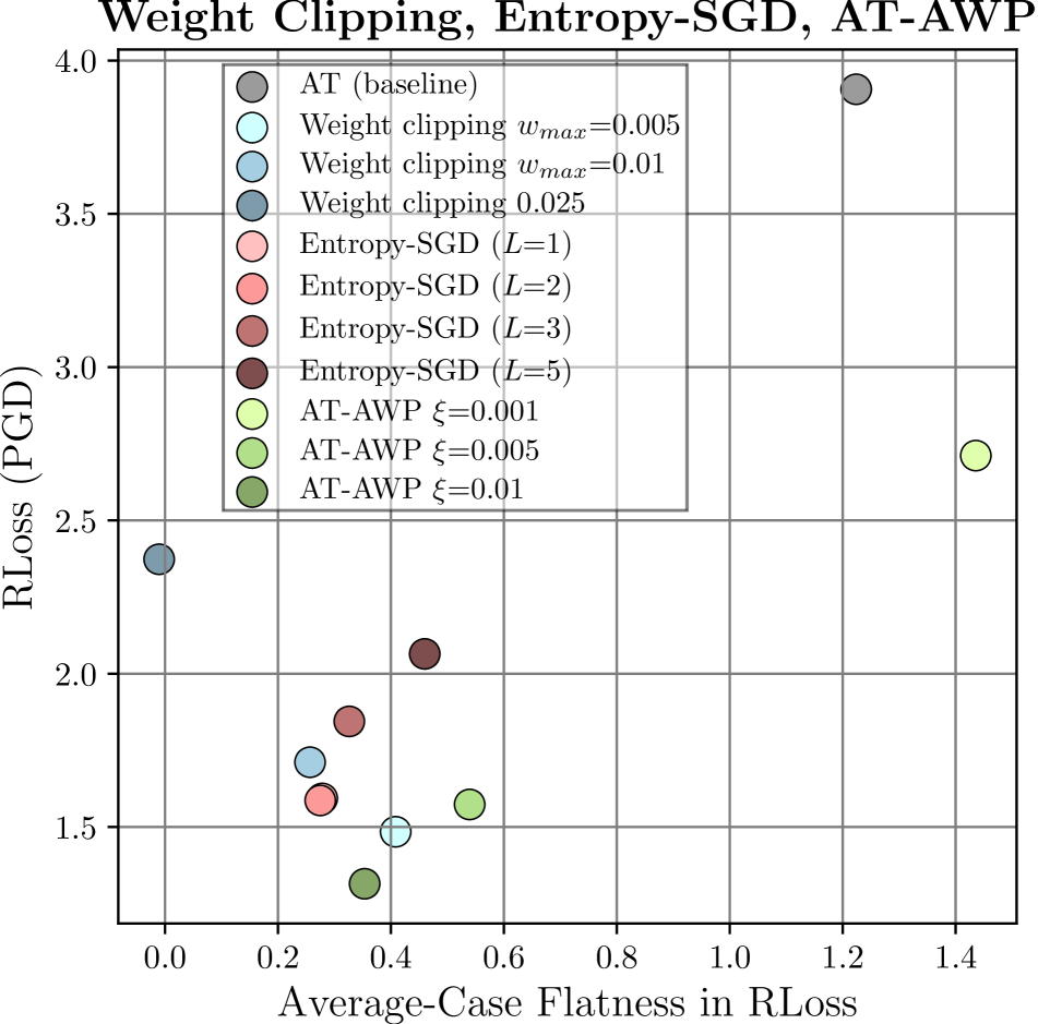
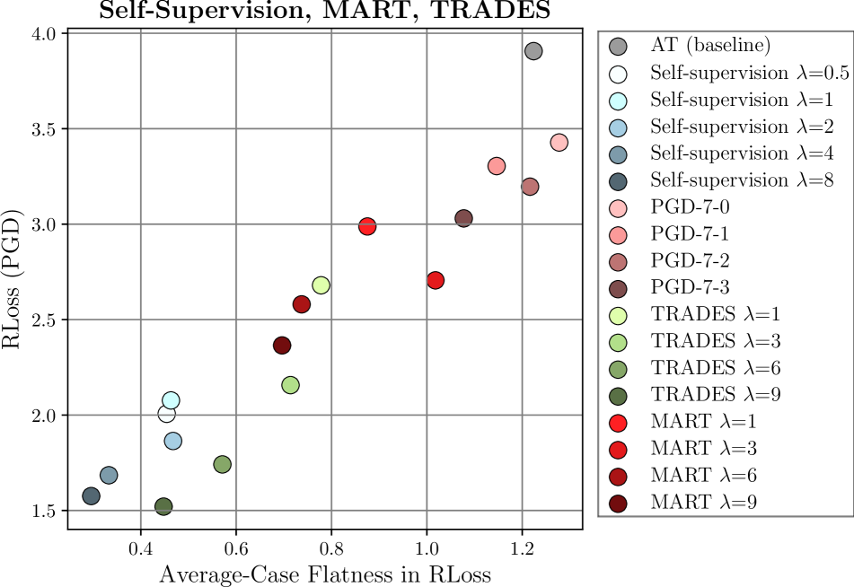
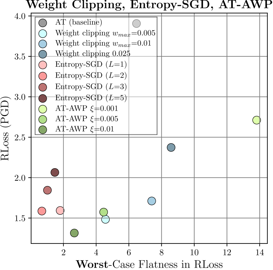
Figure 19: Robustness and Flatness for Varying Hyper-Parameters: Left: RLoss (y-axis) plotted against average-case flatness of RLoss (x-axis) for various groups of methods: learning rate schedules (left), label smoothing/noise and weight decay (middle left), weight clipping, Entropy-SGD and AT-AWP (middle right) as well as AT with self-supervision, MART and TRADES (right). As outlined in Sec. G, we considered multiple hyper-parameter settings per method and show that favorable hyper-parameters in terms of adversarial robustness also result in improved flatness. That is, in most cases, varying hyper-parameters creates (roughly) a diagonal line in these plots. Interestingly, weight clipping can be considered an outlier: adversarial robustness improves while average-case flatness reduces. Right: RLoss (y-axis) plotted against worst-case flatness in RLoss (x-axis). Here, flatness for weight clipping aligns well with RLoss .

Flatness Throughout Training: Fig. 18 shows RLoss (y-axis) plotted against average-case flatness in RLoss (x-axis) throughout training, i.e., over epochs (dark blue to dark red), for methods not shown in the main paper. Strikingly, using higher $\epsilon{=}\nicefrac{{9}}{{255}}$ or alternative activation functions (SiLU [35], GeLU [49] or MiSH [85]) affect neither robust overfitting nor flatness significantly. Interestingly, as discussed in the main paper, label smoothing avoids sharper minima during overfitting, but does not avoid an increased RLoss . Methods that consistently reduce or avoid robust overfitting, e.g., weight clipping, label noise, strong weight decay or AutoAugment, avoid both the increase in RLoss as well as worse flatness. Clearly, the observations from the main paper are confirmed: flatness usually reduces alongside RLoss in robust overfitting.

Flatness Across Hyper-Parameters: In Fig. 19, we consider flatness when changing hyper-parameters of selected methods. As before, we plot RLoss (y-axis) against average-case flatness in RLoss (x-axis) for various groups of methods: learning rate schedules (first column), label smoothing/noise and weight decay (second column), methods explicitly improving flatness, i.e., weight clipping, Entropy-SGD and AT-AWP (third column), as well as self-supervision, MART and TRADES (fourth column). Except for weight clipping, hyper-parameter settings with improved adversarial robustness also favor flatter minima. In most cases, this relationship follows a clear, diagonal line. For weight clipping, in contrast, the relationship is reversed: improved flatness reduces RLoss . Thus, Fig. 19 (fifth column) considers worst-case flatness in RLoss . Here, “stronger” weight clipping improves both robustness and flatness. This supports our discussion in the main paper: methods need at least “some kind” of flatness, average- or worst-case, in order to improve adversarial robustness.

Appendix H Results in Tabular Form

Tab. 5 and 6 report the quantitative results from all our experiments. Besides flatness in RLoss , we also report both average- and worst-case flatness in (clean) Loss . As described in the main paper, we use $\xi=0.5$ for average-case flatness and $\xi=0.003$ for worst-case flatness. In Tab. 5, methods are sorted (in ascending order) by RErr against AutoAttack [25]. Additionally, we split all methods into four groups: good, average, poor and worse robustness at $57\%$, $60\%$ and $62.8\%$ RErr . These thresholds correspond roughly to the $30\%$ and $70\%$ percentile of all methods with $\text{RErr}\leq 62.8\%$. As our AT baseline obtains $62.8\%$ RErr , we group all methods with higher RErr than $62.8\%$ in worse robustness. In Tab. 6, methods are sorted (in ascending order) by RLoss against PGD. Finally, Tab. 3 and 4 report RErr and RLoss , together with our average- and worst-case flatness (of RLoss ) measures for the evaluated, pre-trained models from RobustBench [24].

Model	Test Robustness			Train Robustness			Flatness
(sorted by RLoss on AA)	Err	RErr	RErr	Err	RErr	RErr	Avg	Worst
(PGD = PGD-$20$, $10$ restarts)	(test)	(test)	(test)	(train)	(train)	(train)	RLoss	RLoss
(AA = AutoAttack [26])		(PGD)	(AA)		(PGD)	(AA)
Carmon et al. [16]	10.31	37.6	40.8	1.93	16.8	19.2	0.7	0.34
Engstrom et al. [36]	12.97	45.3	49.2	6.71	33.1	36.3	0.23	0.51
Pang et al. [93]	14.87	36.6	45.8	7.79	20.5	28.6	0.08	0.07
Wang [238]	12.5	37.1	42.8	8.07	24.8	32.1	0.61	0.34
Wong et al. [131]	16.66	54.4	57.6	11.86	44.9	49.2	0.3	0.16
Wu et al. [133]	14.64	41.5	43.9	2.2	14.5	16.5	0.49	0.09
Zhang et al. [148]	15.08	44.1	46.4	7.83	29.9	33.6	0.61	0.43
Zhang et al. [149]	15.48	43	47.2	4.85	26.3	30.1	0.51	0.13

Table 3: RobustBench [24]: Err , RErr and Flatness in RLoss : Err and RErr on train and test examples as well as average- and worst-case flatness in RLoss for pre-trained models from RobustBench. In contrast to Tab. 5, the RobustBench models were obtained using early stopping.

Model	Test Robustness			Train Robustness			Flatness
(sorted by RLoss on AA)	Loss	RLoss	RLoss	Loss	RLoss	RLoss	Avg	Worst
(PGD = PGD-$20$, $10$ restarts)	(test)	(test)	(test)	(train)	(train)	(train)	RLoss	RLoss
(AA = AutoAttack [26])		(PGD)	(AA)		(PGD)	(AA)
Carmon et al. [16]	0.53	1.02	0.63	0.36	0.62	0.41	0.7	0.34
Engstrom et al. [36]	0.44	1.25	0.59	0.29	0.82	0.41	0.23	0.51
Pang et al. [93]	1.84	1.98	1.86	1.8	1.91	1.8	0.08	0.07
Wang [128]	0.64	1.11	0.73	0.54	0.9	0.6	0.61	0.34
Wong et al. [131]	0.57	1.37	0.73	0.46	1.11	0.61	0.3	0.16
Wu et al. [133]	0.63	1.13	0.72	0.37	0.61	0.41	0.49	0.09
Zhang et al. [148]	0.55	1.19	0.66	0.39	0.83	0.48	0.61	0.43
Zhang et al. [149]	0.85	1.27	0.93	0.71	1.01	0.76	0.51	0.13

Table 4: RobustBench [24]: Loss , RLoss and Flatness in RLoss : Loss and RLoss on train and test examples as well as average- and worst-case flatness in RLoss for pre-trained models from RobustBench. In contrast to Tab. 6, the RobustBench models were obtained using early stopping.

Model	Test Robustness			Train Robustness			Early Stopping		Flatness
(sorted by RErr on AA)	Err	RErr	RErr	Err	RErr	RErr	RErr	RErr	Avg	Worst	Avg	Worst
(PGD = PGD-$20$, $10$ restarts)	(test)	(test)	(test)	(train)	(train)	(train)	(stop)	(stop)	Loss	Loss	RLoss	RLoss
(AA = AutoAttack [26])		(PGD)	(AA)		(PGD)	(AA)	(PGD)	(AA)
+Unlabeled	16.96	45.9	48.9	12.6	38.6	43.2	45.3	48.9	0.12	4.64	0.32	1.2
Cyclic $\times 2$	19.66	51.2	53.6	7.64	32.3	35.4	51	53.6	0.09	3.93	0.35	1.5
AutoAugment	16.89	49.5	54.0	12.25	42.8	47.9	49.5	53.5	0.13	15.01	0.49	0.69
AT-AWP $\xi{=}0.01$	21.4	50.7	54.3	13.52	37.4	43.1	48.9	53.6	0.12	6.17	0.35	2.68
AT-AWP $\xi{=}0.005$	20.05	52.5	55	7.34	28.1	31.8	50.8	53.3	0.15	6.98	0.54	4.46
Label noise $\tau{=}0.4$	20.56	52.4	55	9.66	32.8	36.8	51.2	54.8	0.11	3.95	0.21	0.96
TRADES $\lambda{=}9$	23.03	52.4	55	2.92	16.4	18.8	49.7	53	0.19	5.04	0.45	3.08
Cyclic $\times 3$	20.04	53.1	55.2	5.62	26.9	30.6	53.1	55.2	0.1	4.1	0.53	0.93
Cyclic	22.42	53.2	55.4	13.09	39.5	43.5	53.2	55.4	0.07	2.6	0.22	0.41
Label noise $\tau{=}0.5$	22.71	51.3	55.4	15.04	40.4	45.5	51.3	55.4	0.09	0.43	0.16	0.13
Label noise $\tau{=}0.3$	19.9	54.2	56.2	5.47	26.9	30	51.8	55.5	0.15	3.37	0.33	0.93
Weight clipping $w_{max}{=}0.005$	21.39	54.1	56.5	10.19	35.6	39	54.1	56.5	0.74	10.49	0.41	4.58
TRADES $\lambda{=}6$	21.68	55.3	56.7	1.74	13.5	15.8	50.1	53.4	0.21	5.12	0.57	2.26
Cyclic $\times 4$	19.85	55.2	56.9	4.01	23.1	26	55.1	56.9	0.16	6.65	0.62	0.8
Self-supervision $\lambda{=}4$	17.1	55.3	57.1	5.76	41.9	45	55.3	56.8	0.12	5.59	0.34	2.64
Adam	25.84	53.9	57.5	18.87	47.9	52.3	53.9	57.5	0.22	2.65	0.56	0.9
Entropy-SGD ($L{=}2$)	24.53	54.4	57.6	9.03	35.4	38.8	52.6	55.2	0.08	1.76	0.27	0.7
Self-supervision $\lambda{=}1$	15.9	56.9	58.1	1.48	28.3	31.6	55.9	57.5	0.12	6.98	0.46	3.87
Weight decay $0.05$	19.32	56.2	58.1	5.03	29	32.8	52	54.8	0.12	5.77	0.51	3.94
Batch size $8$	17.73	57.1	58.2	3.46	26.8	31.4	55.6	58.2	0.32	24.01	1.55	12.27
Entropy-SGD ($L{=}1$)	25.42	56	58.6	12.79	42.8	46.1	53.2	56.9	0.09	3.24	0.28	1.8
Self-supervision $\lambda{=}0.5$	16.16	58	58.6	1.26	28	30.7	56.7	58.3	0.1	6.48	0.45	3.29
AT-AWP $\xi{=}0.001$	18.75	57.3	58.7	1.34	15.1	18.3	52.1	54.6	0.34	20.42	1.44	13.82
Self-supervision $\lambda{=}2$	15.72	57.4	58.7	2.47	33.4	36.6	55.8	57.7	0.1	21.79	0.47	3.47
MART $\lambda{=}9$	22.06	57	58.8	3.86	16	22	50	55	0.18	8.08	0.7	3.42
Weight decay $0.01$	18.52	57.2	58.9	2.06	20.1	23.2	51.7	55.3	0.25	16.46	0.9	7.19
Batch size $16$	18.12	58.3	59	1.82	20.4	24.5	52.5	55.6	0.33	22.11	1.41	11.39
Self-supervision $\lambda{=}8$	19.6	56.6	59	12.08	50	53.3	56.6	58.6	0.11	3.59	0.29	1.76
TRADES $\lambda{=}3$	20.51	57.7	59.1	0.94	13.4	15.5	52.3	54.9	0.2	19.08	0.71	3.48
Weight decay $0.005$	18.79	58.2	59.4	2.03	20.2	23.9	51.8	54.3	0.26	19.67	1.2	8.35
Label noise $\tau{=}0.2$	19.45	57.5	59.5	2.34	18.8	22.2	50.2	53	0.18	9.79	0.39	1.4
MART $\lambda{=}3$	20.89	58.9	59.6	1.94	14.4	19.2	53.3	57.4	0.17	10.53	1.01	3.99
Weight clipping $w_{max}{=}0.01$	19.15	58	59.6	3.28	21.5	24.8	56.7	58.5	0.66	15.1	0.26	7.41
Learning rate $0.2$	19.17	58.3	59.7	0.46	9.4	12.4	54.3	56.6	0.2	24.41	1.44	5.75
MiSH	19.29	58.9	59.8	0.06	4.5	5.3	51.8	53.7	0.25	10.04	1.58	3.55
“Late” multi-step	20.63	58.5	59.8	1.6	16.4	18.4	54.2	57.8	0.17	5.24	0.81	2.96
SiLU	19.45	59.7	60	0.07	4.8	5.6	51.3	53.7	0.3	9.97	1.68	4.2
Weight averaging ($\tau{=}0.9975$)	19.63	59.7	60	0.19	7.9	10	50.5	53	0.23	15.66	1.29	6
Weight clipping $0.025$	18.91	59.2	60.4	0.73	12.5	15.6	52.1	54.9	0.32	17.4	0	8.61
Batch size $32$	18.72	59.6	60.5	0.56	12	14.6	53.7	55.6	0.18	19.34	1.22	7.88
Entropy-SGD ($L{=}3$)	24	58.5	60.5	5.25	29.9	33.9	56.7	59.3	0.09	2.91	0.33	1.03
Label noise $\tau{=}0.1$	19.39	59	60.8	1.12	14.1	17.5	51.9	55	0.2	16.75	0.69	3.55
Larger $\epsilon{=}9/255$	21.3	60.4	60.9	0.47	8.9	11.1	51.3	53.8	0.21	10.26	1.34	5.85
Label smoothing $\tau{=}0.1$	19.55	59.6	61	0.2	6.4	8.5	52.5	55	0.26	8.87	0.85	2.66
MART $\lambda{=}6$	21.51	58.7	61	3.21	16.1	20.8	49.2	54.7	0.18	13.52	0.74	3.17
Weight averaging ($\tau{=}0.98$)	20.01	60.6	61	0.2	7.6	9.9	54.3	56.3	0.23	12.8	1.37	5.6
Weight decay $0.001$	19.47	59.9	61	0.36	10.4	13.3	52	54.8	0.24	8.36	1.3	6.78
Batch size $64$	19.06	60.5	61.1	0.3	9.2	11.1	51.2	54.4	0.18	23.13	1.14	5.96
GeLU	20.64	60.8	61.1	0.01	2.7	3.2	54.9	56.7	0.23	14.31	1.56	4.13
Label smoothing $\tau{=}0.3$	19.41	59.4	61.2	0.27	5.7	8	51.1	54	0.29	18.42	0.65	2.72
MART $\lambda{=}1$	20.51	59.4	61.2	1.04	11.4	14.7	50.3	55.4	0.17	7.97	0.87	3.1
Weight averaging ($\tau{=}0.99$)	20.41	60.3	61.4	0.19	7.8	9.6	51.7	54.2	0.22	6.12	1.44	4.98
Dropout	18.91	60.5	61.6	0.58	13	16.7	51.2	54.5	0.2	13.81	1.52	7.01
PGD-14	20.8	60.6	61.6	0.22	7.1	9.3	53.6	56.1	0.27	20.9	1.48	5.35
Entropy-SGD ($L{=}5$)	23.48	59.5	61.7	3.01	22.2	25.9	53.2	56.6	0.1	3.57	0.46	1.49
Ignore incorrect	18.4	60.5	61.8	0.06	6.3	9	54.4	56.4	0.21	14.65	1.68	5.93
Learning rate $0.1$	19.23	61.1	61.9	0.26	8.9	11.5	51.9	54.2	0.21	17.63	1.23	5.26
TRADES $\lambda{=}1$	17.54	59.5	61.9	0.15	16.6	20.7	56.6	59.6	0.16	12.68	0.78	4.3
Weight averaging ($\tau{=}0.985$)	20.27	61.7	62.3	0.18	7.4	9.4	55.9	58	0.22	15.66	1.35	6.51
Label smoothing $\tau{=}0.2$	20.07	60.2	62.4	0.26	5.1	7.8	51.9	54.6	0.28	9.94	0.69	2.61
Prevent label leaking	18.38	62.1	62.4	0.38	8.6	10.8	55.3	57.7	0.22	14.62	1.48	6
AT (baseline)	20.2	61	62.8	0.33	8.5	10.7	52.3	54.6	0.21	21.05	1.22	6.49
Const learning rate $0.05$	24.96	60.7	62.9	6.17	32.9	37.8	55.4	58.9	0.09	3.52	0.44	0.9
PGD-5	20.22	61.8	62.9	0.11	7.3	10.4	55.1	57.4	0.17	20.4	1.24	4.19
Batch size $256$	20.86	62.6	63.3	0.28	8.2	10.3	56.9	58.4	0.3	11.22	1.35	8.33
PGD-$7$-$3$	17.17	61.7	63.3	0.08	19.5	25.2	51.3	58.8	0.17	7.4	1.08	5.29
Batch size $512$	22.58	62.9	63.5	0.64	11	14.2	58.6	60	0.48	23.97	1.92	16.22
Learning rate $0.01$	22.83	63	63.5	1.05	15.2	18	57.8	59.7	0.56	23.42	2.25	16.02
No weight decay	23.37	64.8	65.7	0.23	9.2	12.7	57.1	60.3	0.66	21.05	2.53	11.75
PGD-$7$-$0$	14.67	63.8	65.7	0.09	23.7	30	59.4	61.4	0.11	6.86	1.28	2.8
PGD-$7$-$2$	16.19	63.6	65.9	0.1	20.9	28.1	58.3	62.3	0.14	22.81	1.21	2.55
PGD-$7$-$1$	15.02	64.1	67.1	0.11	25.9	34.3	58.8	63.8	0.13	11.71	1.15	2.33
Const learning rate $0.01$	25.87	66.7	67.4	0.67	18.5	20.7	58.4	61	0.33	15.09	1.37	8.27
Const learning rate $0.005$	27.24	68.3	69.2	0.42	15.5	16.7	61.1	65.5	0.59	20.63	2.06	15.74

Table 5: Results: Err , RErr and Flatness in Loss and RLoss . Err and RErr (PGD-$20$ and AutoAttack [25]) on test and train examples, together with average- and worst-case flatness in (clean) Loss and RLoss . Methods sorted by (test) RErr against AutoAttack and split into good, average, poor and worse robustness at $57\%$, $60\%$ and $62.8\%$ RErr , see text.

Model	Test Robustness			Train Robustness			Early Stopping
(sorted by RLoss on PGD)	Loss	RLoss	RLoss	Loss	RLoss	RLoss	RLoss	RLoss
(PGD = PGD-$20$, $10$ restarts)	(test)	(test)	(test)	(train)	(train)	(train)	(stop)	(stop)
(AA = AutoAttack [26])		(PGD)	(AA)		(PGD)	(AA)	(PGD)	(AA)
+Unlabeled	0.57	1.18	0.67	0.47	0.94	0.56	1.18	0.67
AutoAugment	0.58	1.3	0.71	0.48	1.08	0.61	1.3	0.71
AT-AWP $\xi{=}0.01$	0.7	1.31	0.81	0.55	0.99	0.62	1.3	0.81
Cyclic	0.68	1.41	0.8	0.49	0.97	0.58	1.41	0.8
Adam	0.8	1.46	0.89	0.66	1.19	0.74	1.45	0.89
Weight clipping $w_{max}{=}0.005$	0.77	1.48	0.91	0.53	0.99	0.62	1.47	0.9
TRADES $\lambda{=}9$	0.77	1.52	0.9	0.33	0.58	0.37	1.42	0.9
Label noise $\tau{=}0.4$	0.93	1.55	1.05	0.71	1.15	0.8	1.5	1.05
Cyclic $\times 2$	0.6	1.55	0.74	0.32	0.76	0.42	1.55	0.74
AT-AWP $\xi{=}0.005$	0.59	1.57	0.74	0.29	0.66	0.38	1.36	0.74
Self-supervision $\lambda{=}8$	0.59	1.58	0.76	0.43	1.24	0.62	1.57	0.76
Entropy-SGD ($L{=}2$)	0.72	1.59	0.83	0.4	0.87	0.5	1.44	0.83
Label noise $\tau{=}0.5$	1.12	1.59	1.22	1	1.39	1.08	1.59	1.22
Entropy-SGD ($L{=}1$)	0.77	1.59	0.87	0.5	1.06	0.6	1.44	0.87
Label noise $\tau{=}0.3$	0.78	1.62	0.94	0.45	0.91	0.55	1.47	0.94
Weight decay $0.05$	0.61	1.65	0.78	0.28	0.73	0.39	1.33	0.78
Self-supervision $\lambda{=}4$	0.51	1.68	0.71	0.25	1.02	0.45	1.62	0.71
Weight clipping $w_{max}{=}0.01$	0.62	1.71	0.83	0.22	0.61	0.31	1.59	0.83
TRADES $\lambda{=}6$	0.7	1.74	0.86	0.2	0.44	0.25	1.4	0.86
Cyclic $\times 3$	0.6	1.75	0.74	0.24	0.65	0.34	1.59	0.74
Entropy-SGD ($L{=}3$)	0.69	1.84	0.85	0.26	0.72	0.38	1.57	0.85
Self-supervision $\lambda{=}2$	0.47	1.86	0.69	0.13	0.8	0.33	1.53	0.69
Label noise $\tau{=}0.2$	0.68	1.89	0.9	0.22	0.63	0.32	1.4	0.9
Cyclic $\times 4$	0.6	1.9	0.78	0.2	0.57	0.28	1.44	0.78
Const learning rate $0.05$	0.75	1.92	0.89	0.31	0.81	0.43	1.54	0.88
Self-supervision $\lambda{=}0.5$	0.48	2.01	0.71	0.09	0.67	0.27	1.6	0.71
Entropy-SGD ($L{=}5$)	0.71	2.06	0.89	0.18	0.57	0.28	1.5	0.86
Self-supervision $\lambda{=}1$	0.48	2.08	0.72	0.09	0.67	0.27	1.63	0.7
Label smoothing $\tau{=}0.3$	0.77	2.12	1.02	0.15	0.47	0.21	1.46	0.97
TRADES $\lambda{=}3$	0.65	2.16	0.85	0.1	0.34	0.17	1.42	0.83
Batch size $8$	0.56	2.22	0.78	0.17	0.64	0.3	1.86	0.76
Label noise $\tau{=}0.1$	0.63	2.22	0.87	0.1	0.42	0.19	1.37	0.86
Weight decay $0.01$	0.58	2.23	0.78	0.12	0.47	0.22	1.35	0.78
Label smoothing $\tau{=}0.2$	0.71	2.26	0.98	0.09	0.35	0.14	1.44	0.89
MART $\lambda{=}9$	0.7	2.36	0.93	0.24	0.48	0.3	1.41	0.93
Weight clipping $0.025$	0.57	2.37	0.81	0.06	0.32	0.14	1.39	0.81
Weight decay $0.005$	0.58	2.44	0.8	0.11	0.46	0.23	1.43	0.76
Label smoothing $\tau{=}0.1$	0.64	2.48	0.88	0.04	0.24	0.09	1.43	0.8
MART $\lambda{=}6$	0.71	2.58	0.93	0.21	0.45	0.27	1.4	0.93
“Late” multi-step	0.66	2.63	0.87	0.09	0.36	0.17	1.47	0.87
TRADES $\lambda{=}1$	0.56	2.68	0.81	0.04	0.38	0.18	1.74	0.74
MART $\lambda{=}3$	0.69	2.71	0.89	0.14	0.38	0.21	1.48	0.89
AT-AWP $\xi{=}0.001$	0.62	2.71	0.84	0.08	0.34	0.16	1.35	0.78
Batch size $16$	0.57	2.78	0.83	0.1	0.46	0.22	1.63	0.74
Learning rate $0.01$	0.72	2.94	0.96	0.07	0.34	0.16	1.74	0.85
MART $\lambda{=}1$	0.7	2.99	0.94	0.08	0.29	0.15	1.44	0.94
PGD-$7$-$3$	0.55	3.03	0.8	0.04	0.48	0.19	1.7	0.73
PGD-$7$-$2$	0.54	3.2	0.79	0.03	0.48	0.21	2.12	0.71
PGD-$7$-$1$	0.51	3.3	0.75	0.04	0.61	0.25	2.43	0.68
Batch size $512$	0.77	3.41	1.04	0.05	0.27	0.12	1.86	0.85
PGD-$7$-$0$	0.49	3.43	0.74	0.03	0.58	0.21	2.48	0.65
Dropout	0.66	3.44	0.9	0.04	0.3	0.13	1.44	0.76
Const learning rate $0.01$	0.89	3.46	1.07	0.04	0.43	0.17	1.67	0.97
Weight decay $0.001$	0.69	3.52	0.92	0.03	0.24	0.1	1.41	0.77
Batch size $32$	0.67	3.54	0.91	0.04	0.27	0.11	1.69	0.73
Batch size $64$	0.69	3.62	0.93	0.03	0.22	0.09	1.44	0.76
Const learning rate $0.005$	0.97	3.65	1.24	0.04	0.35	0.14	1.62	1.12
MiSH	0.69	3.65	0.92	0.01	0.1	0.04	1.45	0.73
Learning rate $0.1$	0.7	3.65	0.94	0.02	0.19	0.09	1.39	0.79
Learning rate $0.2$	0.72	3.66	0.97	0.03	0.21	0.1	1.67	0.75
Larger $\epsilon{=}9/255$	0.78	3.69	1.01	0.03	0.19	0.09	1.45	0.79
Prevent label leaking	0.67	3.76	0.91	0.02	0.21	0.08	1.74	0.7
SiLU	0.71	3.81	0.96	0.01	0.11	0.04	1.47	0.73
PGD-14	0.76	3.84	1.05	0.02	0.15	0.07	1.52	0.78
Weight averaging ($\tau{=}0.9975$)	0.73	3.88	1	0.02	0.17	0.08	1.34	0.81
AT (baseline)	0.75	3.91	0.99	0.02	0.19	0.08	1.53	0.77
Weight averaging ($\tau{=}0.98$)	0.75	3.94	1.05	0.02	0.16	0.08	1.96	0.8
Weight averaging ($\tau{=}0.985$)	0.75	3.95	1	0.02	0.16	0.07	1.94	0.77
Ignore incorrect	0.71	3.99	0.96	0.01	0.16	0.07	1.65	0.7
Weight averaging ($\tau{=}0.99$)	0.76	3.99	1.07	0.02	0.18	0.07	1.53	0.74
Batch size $256$	0.79	4.02	1.07	0.02	0.18	0.08	1.74	0.81
No weight decay	0.9	4.17	1.15	0.02	0.22	0.1	1.55	0.91
PGD-5	0.77	4.22	0.99	0.01	0.17	0.08	1.62	0.77
GeLU	0.82	4.27	1.06	0	0.06	0.02	1.7	0.79

Table 6: Results: Loss and RLoss . Loss and RLoss (PGD-$20$ and AutoAttack [25]) on test and train examples corresponding to the results in Tab. 5.

References

- [1] Naveed Akhtar and Ajmal S. Mian. Threat of adversarial attacks on deep learning in computer vision: A survey. IEEE Access, 6, 2018.
- [2] Jean-Baptiste Alayrac, Jonathan Uesato, Po-Sen Huang, Alhussein Fawzi, Robert Stanforth, and Pushmeet Kohli. Are labels required for improving adversarial robustness? In NeurIPS, 2019.
- [3] Laurent Amsaleg, James Bailey, Dominique Barbe, Sarah M. Erfani, Michael E. Houle, Vinh Nguyen, and Milos Radovanovic. The vulnerability of learning to adversarial perturbation increases with intrinsic dimensionality. In WIFS, 2017.
- [4] Maksym Andriushchenko and Nicolas Flammarion. Understanding and improving fast adversarial training. In Hugo Larochelle, Marc’Aurelio Ranzato, Raia Hadsell, Maria-Florina Balcan, and Hsuan-Tien Lin, editors, NeurIPS, 2020.
- [5] Anish Athalye and Nicholas Carlini. On the robustness of the CVPR 2018 white-box adversarial example defenses. arXiv.org, abs/1804.03286, 2018.
- [6] Anish Athalye, Nicholas Carlini, and David A. Wagner. Obfuscated gradients give a false sense of security: Circumventing defenses to adversarial examples. arXiv.org, abs/1802.00420, 2018.
- [7] Yogesh Balaji, Tom Goldstein, and Judy Hoffman. Instance adaptive adversarial training: Improved accuracy tradeoffs in neural nets. arXiv.org, abs/1910.08051, 2019.
- [8] Arjun Nitin Bhagoji, Daniel Cullina, and Prateek Mittal. Dimensionality reduction as a defense against evasion attacks on machine learning classifiers. arXiv.org, abs/1704.02654, 2017.
- [9] Battista Biggio and Fabio Roli. Wild patterns: Ten years after the rise of adversarial machine learning. In CCS, 2018.
- [10] Johan Bjorck, Carla P. Gomes, Bart Selman, and Kilian Q. Weinberger. Understanding batch normalization. In NeurIPS, 2018.
- [11] Wieland Brendel and Matthias Bethge. Comment on ”biologically inspired protection of deep networks from adversarial attacks”. arXiv.org, abs/1704.01547, 2017.
- [12] Jacob Buckman, Aurko Roy, Colin Raffel, and Ian Goodfellow. Thermometer encoding: One hot way to resist adversarial examples. In ICLR, 2018.
- [13] Nicholas Carlini and David Wagner. Adversarial examples are not easily detected: Bypassing ten detection methods. In AISec, 2017.
- [14] Nicholas Carlini and David Wagner. Towards evaluating the robustness of neural networks. In SP, 2017.
- [15] Nicholas Carlini and David A. Wagner. Defensive distillation is not robust to adversarial examples. arXiv.org, abs/1607.04311, 2016.
- [16] Yair Carmon, Aditi Raghunathan, Ludwig Schmidt, John C. Duchi, and Percy Liang. Unlabeled data improves adversarial robustness. In NeurIPS, 2019.
- [17] Pratik Chaudhari, Anna Choromanska, Stefano Soatto, Yann LeCun, Carlo Baldassi, Christian Borgs, Jennifer T. Chayes, Levent Sagun, and Riccardo Zecchina. Entropy-sgd: Biasing gradient descent into wide valleys. In ICLR, 2017.
- [18] Pin-Yu Chen, Huan Zhang, Yash Sharma, Jinfeng Yi, and Cho-Jui Hsieh. ZOO: Zeroth order optimization based black-box attacks to deep neural networks without training substitute models. In AISec, 2017.
- [19] Nicholas Cheney, Martin Schrimpf, and Gabriel Kreiman. On the robustness of convolutional neural networks to internal architecture and weight perturbations. arXiv.org, abs/1703.08245, 2017.
- [20] Ching-Tai Chiu, Kishan Mehrotra, Chilukuri K. Mohan, and Sanjay Ranka. Training techniques to obtain fault-tolerant neural networks. In Annual International Symposium on Fault-Tolerant Computing, 1994.
- [21] Safa Cicek and Stefano Soatto. Input and weight space smoothing for semi-supervised learning. In ICCV Workshops, 2019.
- [22] Jeremy M. Cohen, Elan Rosenfeld, and J. Zico Kolter. Certified adversarial robustness via randomized smoothing. arXiv.org, abs/1902.02918, 2019.
- [23] Francesco Croce, Maksym Andriushchenko, and Matthias Hein. Provable robustness of relu networks via maximization of linear regions. arXiv.org, abs/1810.07481, 2018.
- [24] Francesco Croce, Maksym Andriushchenko, Vikash Sehwag, Nicolas Flammarion, Mung Chiang, Prateek Mittal, and Matthias Hein. Robustbench: a standardized adversarial robustness benchmark. arXiv.org, abs/2010.09670, 2020.
- [25] Francesco Croce and Matthias Hein. Reliable evaluation of adversarial robustness with an ensemble of diverse parameter-free attacks. In ICML, 2020.
- [26] Francesco Croce and Matthias Hein. Reliable evaluation of adversarial robustness with an ensemble of diverse parameter-free attacks. arXiv.org, abs/2003.01690, 2020.
- [27] Ekin Dogus Cubuk, Barret Zoph, Dandelion Mané, Vijay Vasudevan, and Quoc V. Le. Autoaugment: Learning augmentation policies from data. arXiv.org, abs/1805.09501, 2018.
- [28] Dipti Deodhare, M. Vidyasagar, and S. Sathiya Keerthi. Synthesis of fault-tolerant feedforward neural networks using minimax optimization. TNN, 9(5):891–900, 1998.
- [29] Terrance Devries and Graham W. Taylor. Improved regularization of convolutional neural networks with cutout. arXiv.org, abs/1708.04552, 2017.
- [30] Gavin Weiguang Ding, Yash Sharma, Kry Yik Chau Lui, and Ruitong Huang. MMA training: Direct input space margin maximization through adversarial training. In ICLR, 2020.
- [31] Laurent Dinh, Razvan Pascanu, Samy Bengio, and Yoshua Bengio. Sharp minima can generalize for deep nets. In ICML, 2017.
- [32] Yinpeng Dong, Fangzhou Liao, Tianyu Pang, Hang Su, Jun Zhu, Xiaolin Hu, and Jianguo Li. Boosting adversarial attacks with momentum. In CVPR, 2018.
- [33] Vasisht Duddu, D. Vijay Rao, and Valentina E. Balas. Adversarial fault tolerant training for deep neural networks. arXiv.org, abs/1907.03103, 2019.
- [34] Jacob Dumford and Walter J. Scheirer. Backdooring convolutional neural networks via targeted weight perturbations. arXiv.org, abs/1812.03128, 2018.
- [35] Stefan Elfwing, Eiji Uchibe, and Kenji Doya. Sigmoid-weighted linear units for neural network function approximation in reinforcement learning. NN, 107, 2018.
- [36] Logan Engstrom, Andrew Ilyas, Hadi Salman, Shibani Santurkar, and Dimitris Tsipras. Robustness (python library), 2019.
- [37] Farzan Farnia, Jesse M. Zhang, and David Tse. Generalizable adversarial training via spectral normalization. In ICLR, 2019.
- [38] Reuben Feinman, Ryan R Curtin, Saurabh Shintre, and Andrew B Gardner. Detecting adversarial samples from artifacts. arXiv.org, abs/1703.00410, 2017.
- [39] Timon Gehr, Matthew Mirman, Dana Drachsler-Cohen, Petar Tsankov, Swarat Chaudhuri, and Martin T. Vechev. AI2: safety and robustness certification of neural networks with abstract interpretation. In SP, pages 3–18, 2018.
- [40] Ian J Goodfellow, Jonathon Shlens, and Christian Szegedy. Explaining and harnessing adversarial examples. arXiv.org, abs/1412.6572, 2014.
- [41] Sven Gowal, Krishnamurthy Dvijotham, Robert Stanforth, Rudy Bunel, Chongli Qin, Jonathan Uesato, Relja Arandjelovic, Timothy A. Mann, and Pushmeet Kohli. On the effectiveness of interval bound propagation for training verifiably robust models. arXiv.org, abs/1810.12715, 2018.
- [42] Sven Gowal, Chongli Qin, Jonathan Uesato, Timothy A. Mann, and Pushmeet Kohli. Uncovering the limits of adversarial training against norm-bounded adversarial examples. arXiv.org, abs/2010.03593, 2020.
- [43] Edward Grefenstette, Robert Stanforth, Brendan O’Donoghue, Jonathan Uesato, Grzegorz Swirszcz, and Pushmeet Kohli. Strength in numbers: Trading-off robustness and computation via adversarially-trained ensembles. arXiv.org, abs/1811.09300, 2018.
- [44] Kathrin Grosse, Praveen Manoharan, Nicolas Papernot, Michael Backes, and Patrick McDaniel. On the (statistical) detection of adversarial examples. arXiv.org, abs/1702.06280, 2017.
- [45] Kaiming He, Xiangyu Zhang, Shaoqing Ren, and Jian Sun. Deep residual learning for image recognition. In CVPR, 2016.
- [46] Warren He, James Wei, Xinyun Chen, Nicholas Carlini, and Dawn Song. Adversarial example defense: Ensembles of weak defenses are not strong. In USENIX Workshops, 2017.
- [47] Zhezhi He, Adnan Siraj Rakin, Jingtao Li, Chaitali Chakrabarti, and Deliang Fan. Defending and harnessing the bit-flip based adversarial weight attack. In CVPR, 2020.
- [48] Matthias Hein and Maksym Andriushchenko. Formal guarantees on the robustness of a classifier against adversarial manipulation. In NeurIPS, 2017.
- [49] Dan Hendrycks and Kevin Gimpel. Bridging nonlinearities and stochastic regularizers with gaussian error linear units. arXiv.org, abs/1606.08415, 2016.
- [50] Dan Hendrycks, Mantas Mazeika, Saurav Kadavath, and Dawn Song. Using self-supervised learning can improve model robustness and uncertainty. In NeurIPS, 2019.
- [51] S. Hochreiter and J. Schmidhuber. Flat minima. NC, 9, 1997.
- [52] Ruitong Huang, Bing Xu, Dale Schuurmans, and Csaba Szepesvári. Learning with a strong adversary. arXiv.org, abs/1511.03034, 2015.
- [53] J. Hwang, Youngwan Lee, Sungchan Oh, and Yu-Seok Bae. Adversarial training with stochastic weight average. arXiv.org, abs/2009.10526, 2020.
- [54] Andrew Ilyas, Logan Engstrom, and Aleksander Madry. Prior convictions: Black-box adversarial attacks with bandits and priors. arXiv.org, abs/1807.07978, 2018.
- [55] Andrew Ilyas, Ajil Jalal, Eirini Asteri, Constantinos Daskalakis, and Alexandros G. Dimakis. The robust manifold defense: Adversarial training using generative models. arXiv.org, abs/1712.09196, 2017.
- [56] Sergey Ioffe and Christian Szegedy. Batch normalization: Accelerating deep network training by reducing internal covariate shift. In ICML, 2015.
- [57] Pavel Izmailov, Dmitrii Podoprikhin, Timur Garipov, Dmitry P. Vetrov, and Andrew Gordon Wilson. Averaging weights leads to wider optima and better generalization. In UAI, 2018.
- [58] Daniel Jakubovitz and Raja Giryes. Improving DNN robustness to adversarial attacks using jacobian regularization. arXiv.org, abs/1803.08680, 2018.
- [59] Yujie Ji, Xinyang Zhang, Shouling Ji, Xiapu Luo, and Ting Wang. Model reuse attacks on deep learning systems. In CCS, 2018.
- [60] Yiding Jiang, Behnam Neyshabur, Hossein Mobahi, Dilip Krishnan, and Samy Bengio. Fantastic generalization measures and where to find them. In ICLR, 2020.
- [61] Harini Kannan, Alexey Kurakin, and Ian J. Goodfellow. Adversarial logit pairing. arXiv.org, abs/1803.06373, 2018.
- [62] Nitish Shirish Keskar, Dheevatsa Mudigere, Jorge Nocedal, Mikhail Smelyanskiy, and Ping Tak Peter Tang. On large-batch training for deep learning: Generalization gap and sharp minima. In ICLR, 2017.
- [63] Marc Khoury and Dylan Hadfield-Menell. On the geometry of adversarial examples. arXiv.org, abs/1811.00525, 2018.
- [64] Diederik P. Kingma and Jimmy Ba. Adam: A method for stochastic optimization. In ICLR, 2015.
- [65] Alex Krizhevsky. Learning multiple layers of features from tiny images. Technical report, 2009.
- [66] Aounon Kumar, A. Levine, S. Feizi, and T. Goldstein. Certifying confidence via randomized smoothing. ArXiv, abs/2009.08061, 2020.
- [67] Alexey Kurakin, Ian Goodfellow, and Samy Bengio. Adversarial examples in the physical world. arXiv.org, abs/1607.02533, 2016.
- [68] Alexey Kurakin, Ian Goodfellow, and Samy Bengio. Adversarial machine learning at scale. arXiv.org, abs/1611.01236, 2016.
- [69] Cassidy Laidlaw and Soheil Feizi. Playing it safe: Adversarial robustness with an abstain option. arXiv.org, abs/1911.11253, 2019.
- [70] Alex Lamb, Jonathan Binas, Anirudh Goyal, Dmitriy Serdyuk, Sandeep Subramanian, Ioannis Mitliagkas, and Yoshua Bengio. Fortified networks: Improving the robustness of deep networks by modeling the manifold of hidden representations. arXiv.org, abs/1804.02485, 2018.
- [71] Alex Lamb, Vikas Verma, Juho Kannala, and Yoshua Bengio. Interpolated adversarial training: Achieving robust neural networks without sacrificing too much accuracy. In AISec, 2019.
- [72] Guang-He Lee, David Alvarez-Melis, and Tommi S. Jaakkola. Towards robust, locally linear deep networks. arXiv.org, abs/1907.03207, 2019.
- [73] Hao Li, Zheng Xu, G. Taylor, and T. Goldstein. Visualizing the loss landscape of neural nets. In NeurIPS, 2018.
- [74] Fangzhou Liao, Ming Liang, Yinpeng Dong, Tianyu Pang, Xiaolin Hu, and Jun Zhu. Defense against adversarial attacks using high-level representation guided denoiser. In CVPR, 2018.
- [75] Tao Lin, Sebastian U. Stich, Kumar Kshitij Patel, and Martin Jaggi. Don’t use large mini-batches, use local SGD. In ICLR, 2020.
- [76] Xuanqing Liu, Minhao Cheng, Huan Zhang, and Cho-Jui Hsieh. Towards robust neural networks via random self-ensemble. arXiv.org, abs/1712.00673, 2017.
- [77] Xuanqing Liu, Yao Li, Chongruo Wu, and Cho-Jui Hsieh. Adv-bnn: Improved adversarial defense through robust bayesian neural network. In ICLR, 2019.
- [78] Bo Luo, Yannan Liu, Lingxiao Wei, and Qiang Xu. Towards imperceptible and robust adversarial example attacks against neural networks. In AAAI, 2018.
- [79] Xingjun Ma, Bo Li, Yisen Wang adn Sarah M. Erfani, Sudanthi Wijewickrema, Michael E. Houle, Grant Schoenebeck, Dawn Song, and James Bailey. Characterizing adversarial subspaces using local intrinsic dimensionality. arXiv.org, abs/1801.02613, 2018.
- [80] Aleksander Madry, Aleksandar Makelov, Ludwig Schmidt, Dimitris Tsipras, and Adrian Vladu. Towards deep learning models resistant to adversarial attacks. arXiv.org, abs/1706.06083, 2017.
- [81] Aleksander Madry, Aleksandar Makelov, Ludwig Schmidt, Dimitris Tsipras, and Adrian Vladu. Towards deep learning models resistant to adversarial attacks. ICLR, 2018.
- [82] Pratyush Maini, Eric Wong, and J. Zico Kolter. Adversarial robustness against the union of multiple perturbation models. ICML, 2020.
- [83] Jan Hendrik Metzen, Tim Genewein, Volker Fischer, and Bastian Bischoff. On detecting adversarial perturbations. arXiv.org, abs/1702.04267, 2017.
- [84] Matthew Mirman, Timon Gehr, and Martin T. Vechev. Differentiable abstract interpretation for provably robust neural networks. In ICML, pages 3575–3583, 2018.
- [85] Diganta Misra. Mish: A self regularized non-monotonic activation function. In BMVC, 2020.
- [86] Takeru Miyato, Shin-ichi Maeda, Masanori Koyama, Ken Nakae, and Shin Ishii. Distributional smoothing with virtual adversarial training. ICLR, 2016.
- [87] Seyed-Mohsen Moosavi-Dezfooli, Alhussein Fawzi, and Pascal Frossard. Deepfool: A simple and accurate method to fool deep neural networks. In CVPR, 2016.
- [88] Nina Narodytska and Shiva Prasad Kasiviswanathan. Simple black-box adversarial attacks on deep neural networks. In CVPR Workshops, 2017.
- [89] Aran Nayebi and Surya Ganguli. Biologically inspired protection of deep networks from adversarial attacks. arXiv.org, abs/1703.09202, 2017.
- [90] Chalapathy Neti, Michael H. Schneider, and Eric D. Young. Maximally fault tolerant neural networks. TNN, 3(1):14–23, 1992.
- [91] Behnam Neyshabur, Srinadh Bhojanapalli, David McAllester, and Nati Srebro. Exploring generalization in deep learning. In NeurIPS, 2017.
- [92] Tianyu Pang, Xian Yang, Yinpeng Dong, Hang Su, and Jun Zhu. Bag of tricks for adversarial training. arXiv.org, abs/2010.00467, 2020.
- [93] Tianyu Pang, Xiao Yang, Yinpeng Dong, Taufik Xu, Jun Zhu, and Hang Su. Boosting adversarial training with hypersphere embedding. In NeurIPS, 2020.
- [94] Nicolas Papernot, Patrick D. McDaniel, Somesh Jha, Matt Fredrikson, Z. Berkay Celik, and Ananthram Swami. The limitations of deep learning in adversarial settings. In SP, 2016.
- [95] Adam Paszke, Sam Gross, Soumith Chintala, Gregory Chanan, Edward Yang, Zachary DeVito, Zeming Lin, Alban Desmaison, Luca Antiga, and Adam Lerer. Automatic differentiation in pytorch. In NeurIPS Workshops, 2017.
- [96] Rama Chellappa Pouya Samangouei, Maya Kabkab. Defense-GAN: Protecting classifiers against adversarial attacks using generative models. ICLR, 2018.
- [97] Vinay Uday Prabhu, Dian Ang Yap, Joyce Xu, and J. Whaley. Understanding adversarial robustness through loss landscape geometries. arXiv.org, abs/1907.09061, 2019.
- [98] Aaditya Prakash, Nick Moran, Solomon Garber, Antonella DiLillo, and James A. Storer. Protecting JPEG images against adversarial attacks. In DCC, 2018.
- [99] Chongli Qin, James Martens, Sven Gowal, Dilip Krishnan, Krishnamurthy Dvijotham, Alhussein Fawzi, Soham De, Robert Stanforth, and Pushmeet Kohli. Adversarial robustness through local linearization. In NeurIPS, 2019.
- [100] Aditi Raghunathan, Sang Michael Xie, Fanny Yang, John C. Duchi, and Percy Liang. Adversarial training can hurt generalization. arXiv.org, abs/1906.06032, 2019.
- [101] Faiz Ur Rahman, Bhavan Vasu, and Andreas E. Savakis. Resilience and self-healing of deep convolutional object detectors. In ICIP, 2018.
- [102] Adnan Siraj Rakin, Zhezhi He, and Deliang Fan. Bit-flip attack: Crushing neural network with progressive bit search. In ICCV, 2019.
- [103] Leslie Rice, Eric Wong, and J. Zico Kolter. Overfitting in adversarially robust deep learning. In ICML, 2020.
- [104] Andrew Slavin Ross and Finale Doshi-Velez. Improving the adversarial robustness and interpretability of deep neural networks by regularizing their input gradients. In AAAI, 2018.
- [105] Vivek B. S. and R. Venkatesh Babu. Single-step adversarial training with dropout scheduling. In CVPR, 2020.
- [106] Shibani Santurkar, Dimitris Tsipras, Andrew Ilyas, and Aleksander Madry. How does batch normalization help optimization? In NeurIPS, 2018.
- [107] Sayantan Sarkar, Ankan Bansal, Upal Mahbub, and Rama Chellappa. UPSET and ANGRI : Breaking high performance image classifiers. arXiv.org, abs/1707.01159, 2017.
- [108] Ludwig Schmidt, Shibani Santurkar, Dimitris Tsipras, Kunal Talwar, and Aleksander Madry. Adversarially robust generalization requires more data. In NeurIPS, 2018.
- [109] Lukas Schott, Jonas Rauber, Wieland Brendel, and Matthias Bethge. Robust perception through analysis by synthesis. arXiv.org, abs/1805.09190, 2018.
- [110] Shiwei Shen, Guoqing Jin, Ke Gao, and Yongdong Zhang. Ape-gan: Adversarial perturbation elimination with gan. arXiv.org, abs/1707.05474, 2017.
- [111] Samuel Henrique Silva and Peyman Najafirad. Opportunities and challenges in deep learning adversarial robustness: A survey. arXiv.org, abs/2007.00753, 2020.
- [112] Carl-Johann Simon-Gabriel, Yann Ollivier, Bernhard Schölkopf, Léon Bottou, and David Lopez-Paz. Adversarial vulnerability of neural networks increases with input dimension. arXiv.org, abs/1802.01421, 2018.
- [113] Gagandeep Singh, Timon Gehr, Matthew Mirman, Markus Püschel, and Martin T. Vechev. Fast and effective robustness certification. In NeurIPS, pages 10825–10836, 2018.
- [114] Vasu Singla, Sahil Singla, David Jacobs, and Soheil Feizi. Low curvature activations reduce overfitting in adversarial training. arXiv.org, abs/2102.07861, 2021.
- [115] Kihyuk Sohn, David Berthelot, C. Li, Zizhao Zhang, N. Carlini, E. D. Cubuk, Alex Kurakin, Han Zhang, and Colin Raffel. Fixmatch: Simplifying semi-supervised learning with consistency and confidence. arXiv.org, abs/2001.07685, 2020.
- [116] Thilo Strauss, Markus Hanselmann, Andrej Junginger, and Holger Ulmer. Ensemble methods as a defense to adversarial perturbations against deep neural networks. arXiv.org, abs/1709.03423, 2017.
- [117] David Stutz, Nandhini Chandramoorthy, Matthias Hein, and Bernt Schiele. Bit error robustness for energy-efficient dnn accelerators. In MLSys, 2021.
- [118] David Stutz, Matthias Hein, and Bernt Schiele. Disentangling adversarial robustness and generalization. CVPR, 2019.
- [119] David Stutz, Matthias Hein, and Bernt Schiele. Confidence-calibrated adversarial training: Generalizing to unseen attacks. In ICML, 2020.
- [120] Jiawei Su, Danilo Vasconcellos Vargas, and Kouichi Sakurai. One pixel attack for fooling deep neural networks. arXiv.org, abs/1710.08864, 2017.
- [121] Christian Szegedy, Vincent Vanhoucke, Sergey Ioffe, Jonathon Shlens, and Zbigniew Wojna. Rethinking the inception architecture for computer vision. In CVPR, 2016.
- [122] Christian Szegedy, Wojciech Zaremba, Ilya Sutskever, Joan Bruna, Dumitru Erhan, Ian Goodfellow, and Rob Fergus. Intriguing properties of neural networks. arXiv.org, abs/1312.6199, 2013.
- [123] Christian Szegedy, Wojciech Zaremba, Ilya Sutskever, Joan Bruna, Dumitru Erhan, Ian J. Goodfellow, and Rob Fergus. Intriguing properties of neural networks. In ICLR, 2014.
- [124] César Torres-Huitzil and Bernard Girau. Fault and error tolerance in neural networks: A review. IEEE Access, 5, 2017.
- [125] Florian Tramèr and Dan Boneh. Adversarial training and robustness for multiple perturbations. In NeurIPS, 2019.
- [126] Florian Tramèr, Alexey Kurakin, Nicolas Papernot, Dan Boneh, and Patrick D. McDaniel. Ensemble adversarial training: Attacks and defenses. ICLR, 2018.
- [127] Dimitris Tsipras, Shibani Santurkar, Logan Engstrom, Alexander Turner, and Aleksander Madry. Robustness may be at odds with accuracy. In ICLR, 2019.
- [128] Yisen Wang, Difan Zou, Jinfeng Yi, James Bailey, Xingjun Ma, and Quanquan Gu. Improving adversarial robustness requires revisiting misclassified examples. In ICLR, 2020.
- [129] Tsui-Wei Weng, Pu Zhao, Sijia Liu, Pin-Yu Chen, Xue Lin, and Luca Daniel. Towards certificated model robustness against weight perturbations. In AAAI, 2020.
- [130] Eric Wong and J. Zico Kolter. Provable defenses against adversarial examples via the convex outer adversarial polytope. In ICML, 2018.
- [131] Eric Wong, Leslie Rice, and J. Zico Kolter. Fast is better than free: Revisiting adversarial training. In ICLR, 2020.
- [132] Eric Wong, Leslie Rice, and J. Zico Kolter. Fast is better than free: Revisiting adversarial training. arXiv.org, abs/2001.03994, 2020.
- [133] Dongxian Wu, Shu-Tao Xia, and Yisen Wang. Adversarial weight perturbation helps robust generalization. In NeurIPS, 2020.
- [134] Jiajun Wu, Chengkai Zhang, Tianfan Xue, Bill Freeman, and Josh Tenenbaum. Learning a probabilistic latent space of object shapes via 3d generative-adversarial modeling. In NeurIPS, 2016.
- [135] Xi Wu, Uyeong Jang, Jiefeng Chen, Lingjiao Chen, and Somesh Jha. Reinforcing adversarial robustness using model confidence induced by adversarial training. In ICML, 2018.
- [136] Cihang Xie, Jianyu Wang, Zhishuai Zhang, Zhou Ren, and Alan L. Yuille. Mitigating adversarial effects through randomization. ICLR, 2018.
- [137] Han Xu, Yao Ma, Haochen Liu, Debayan Deb, Hui Liu, Jiliang Tang, and Anil K. Jain. Adversarial attacks and defenses in images, graphs and text: A review. arXiv.org, abs/1909.08072, 2019.
- [138] Greg Yang, Tony Duan, Edward Hu, Hadi Salman, Ilya P. Razenshteyn, and Jerry Li. Randomized smoothing of all shapes and sizes. arXiv.org, abs/2002.08118, 2020.
- [139] Zhewei Yao, Amir Gholami, Qi Lei, Kurt Keutzer, and Michael W. Mahoney. Hessian-based analysis of large batch training and robustness to adversaries. In NeurIPS, 2018.
- [140] Nanyang Ye and Zhanxing Zhu. Bayesian adversarial learning. In NeurIPS, 2018.
- [141] F. Yu, C. Liu, Yanzhi Wang, Liang Zhao, and X. Chen. Interpreting adversarial robustness: A view from decision surface in input space. arXiv.org, abs/1810.00144, 2018.
- [142] Xiaoyong Yuan, Pan He, Qile Zhu, Rajendra Rana Bhat, and Xiaolin Li. Adversarial examples: Attacks and defenses for deep learning. arXiv.org, abs/1712.07107, 2017.
- [143] Sergey Zagoruyko and Nikos Komodakis. Wide residual networks. In BMVC, 2016.
- [144] Valentina Zantedeschi, Maria-Irina Nicolae, and Ambrish Rawat. Efficient defenses against adversarial attacks. In AISec, 2017.
- [145] Dinghuai Zhang, Tianyuan Zhang, Yiping Lu, Zhanxing Zhu, and Bin Dong. You only propagate once: Accelerating adversarial training via maximal principle. In NeurIPS.
- [146] Huan Zhang, Hongge Chen, Chaowei Xiao, Bo Li, Duane S. Boning, and Cho-Jui Hsieh. Towards stable and efficient training of verifiably robust neural networks. arXiv.org, abs/1906.06316, 2019.
- [147] Huan Zhang, Tsui-Wei Weng, Pin-Yu Chen, Cho-Jui Hsieh, and Luca Daniel. Efficient neural network robustness certification with general activation functions. In NeurIPS, pages 4944–4953, 2018.
- [148] Hongyang Zhang, Yaodong Yu, Jiantao Jiao, Eric P. Xing, Laurent El Ghaoui, and Michael I. Jordan. Theoretically principled trade-off between robustness and accuracy. In ICML, 2019.
- [149] Jingfeng Zhang, Xilie Xu, Bo Han, Gang Niu, Lizhen Cui, Masashi Sugiyama, and Mohan S. Kankanhalli. Attacks which do not kill training make adversarial learning stronger. In ICML, 2020.
- [150] Jingfeng Zhang, Xilie Xu, Bo Han, Gang Niu, Li zhen Cui, Masashi Sugiyama, and Mohan Kankanhalli. Attacks which do not kill training make adversarial learning stronger. arXiv.org, abs/2002.11242, 2020.
- [151] Yaowei Zheng, Richong Zhang, and Yongyi Mao. Regularizing neural networks via adversarial model perturbation. arXiv.org, abs/2010.04925, 2020.