Larger-Context Tagging: When and Why Does It Work?

Abstract

The development of neural networks and pretraining techniques has spawned many sentence-level tagging systems that achieved superior performance on typical benchmarks. However, a relatively less discussed topic is what if more context information is introduced into current top-scoring tagging systems. Although several existing works have attempted to shift tagging systems from sentence-level to document-level, there is still no consensus conclusion about when and why it works, which limits the applicability of the larger-context approach in tagging tasks. In this paper, instead of pursuing a state-of-the-art tagging system by architectural exploration, we focus on investigating when and why the larger-context training, as a general strategy, can work.

To this end, we conduct a thorough comparative study on four proposed aggregators for context information collecting and present an attribute-aided evaluation method to interpret the improvement brought by larger-context training. Experimentally, we set up a testbed based on four tagging tasks and thirteen datasets. Hopefully, our preliminary observations can deepen the understanding of larger-context training and enlighten more follow-up works on the use of contextual information. We have released all relevant codes for future researchers to run similar analyses: https://github.com/jlfu/larger-context.

1 Introduction

The rapid development of deep neural models has shown impressive performances on sequence tagging tasks that aim to assign labels to each token of an input sequence Sang and De Meulder (2003); Lample et al. (2016); Ma and Hovy (2016). More recently, the use of unsupervised pre-trained models Akbik et al. (2018, 2019); Peters et al. (2018); Devlin et al. (2018) (especially contextualized version) has driven state-of-the-art performance to a new level. Among these works, researchers frequently choose the boundary with the granularity of sentences for tagging tasks (i.e., sentence-level tagging) Huang et al. (2015); Chiu and Nichols (2015); Ma and Hovy (2016); Lample et al. (2016). Undoubtedly, as a transient, sentence-level setting enables us to develop numerous successful tagging systems, nevertheless the task itself should have not be defined as sentence-level but for simplifying the learning process for machine learning models. Naturally, it would be interesting to see what if larger-context information (e.g., taking information of neighbor sentences into account) is introduced to modern top-scoring systems, which have shown superior performance under the sentence-level setting. A small number of works have made seminal exploration in this direction, in which part of works show significant improvement of larger-context Luo et al. (2020); Xu et al. (2019) while others don’t Hu et al. (2020, 2019); Luo et al. (2018). Therefore, it’s still unclear when and why larger-context training is beneficial for tagging tasks. In this paper, we try to figure it out by asking the following three research questions:

Q1: How do different integration ways of larger-context information influence the system’s performance? The rapid development of neural networks provides us with diverse flavors of neural components to aggregate larger-context information, which, for example, can be structured as a sequential topology by recurrent neural networks Ma and Hovy (2016); Lample et al. (2016) (RNNs) or graph topology by graph neural networks Kipf and Welling (2016); Schlichtkrull et al. (2018).

Understanding the discrepancies of these aggregators can help us reach a more generalized conclusion about the effectiveness of larger-context training. To this end, we study larger-context aggregators with three different structural priors (defined in Sec. 3.2) and comprehensively evaluate their efficacy.

Q2: Can the larger-context training easily play to its strengths with the help of recently arising contextualized pre-trained models  Akbik et al. (2018, 2019); Peters et al. (2018); Devlin et al. (2018) (e.g. BERT)? The contextual modeling power of these pre-trained methods makes it worth looking at its effect on larger-context training. In this work, we take BERT as a case study and assess its effectiveness quantitatively and qualitatively.

Q3: If improvements could be observed, where does the gain come and how do different characteristics of datasets affect the amount of gain? Instead of simply figuring out whether larger-context training could work, we also try to interpret its gains. Specifically, we propose to use fine-grained evaluation to explain where the improvement comes from and why different datasets exhibit discrepant gains.

Overall, the first two questions aim to explore when larger-context training can work while the third question addresses why. Experimentally, we try to answer these questions by conducting a comprehensive analysis, which involves four tagging tasks and thirteen datasets. Our main observations are summarized in Sec. 8.  Furthermore, we show, with the help of these observations, it’s easier to adapt larger-context training to modern top-performing tagging systems with significant gains. We brief our contributions below:

1) We try to bridge the gap by asking three research questions, between the increasing top-performing sentence-level tagging systems and insufficient understanding of larger-context training, encouraging future research to explore more larger-context tagging systems. 2) We systematically investigate four aggregators for larger-context and present an attribute-aided evaluation methodology to interpret the relative advantages of them, and why they can work (Sec. 3.2). 3) Based on some of our observations, we adapt larger-context training to five modern top-scoring systems in the NER task and observe that all larger-context enhanced models can achieve significant improvement (Sec. 6). Encouragingly , with the help of larger-context training, the performance of Akbik et al. (2018) on the WB (OntoNotes5.0-WB) dataset can be improved by a 10.78 $F1$ score.

2 Task, Dataset, and Model

We first explicate the definition of tagging task and then describe several popular datasets as well as typical methods of this task.

2.1 Task Definition

Sequence tagging aims to assign one of the pre-defined labels to each token in a sequence. In this paper, we consider four types of concrete tasks: Named Entity Recognition (NER), Chinese Word Segmentation (CWS), Part-of-Speech (POS) tagging, and Chunking.

2.2 Datasets

The datasets used in our paper are naturally ordered without random shuffling according to the paper that constructed these datasets, except for WNUT-2016 dataset.

Named Entity Recognition (NER) We consider two well-established benchmarks: CoNLL-2003 (CN03) and OntoNotes 5.0. OntoNotes 5.0 is collected from six different genres: broadcast conversation (BC), broadcast news (BN), magazine (MZ), newswire (NW), telephone conversation (TC), and web data (WB). Since each domain of OntoNotes 5.0 has its nature, we follow previous works Durrett and Klein (2014); Chiu and Nichols (2016); Ghaddar and Langlais (2018) that utilize different domains of this dataset, which also paves the way for our fine-grained analysis.

Chinese Word Segmentation (CWS) We use four mainstream datasets from SIGHAN2005 and SIGHAN2008, in which CITYU is traditional Chinese, while PKU, NCC, and SXU are simplified ones.

Chunking (Chunk) CoNLL-2000 (CN00) is a benchmark dataset for text chunking.

Part-of-Speech (POS) We use the Penn Treebank (PTB) III dataset for POS tagging.

2.3 Neural Tagging Models

Despite the emergence of a bunch of architectural explorations Ma and Hovy (2016); Lample et al. (2016); Yang et al. (2018); Peters et al. (2018); Akbik et al. (2018); Devlin et al. (2018) for sequence tagging, two general frameworks can be summarized: (i) cEnc-wEnc-CRF consists of the word-level encoder, sentence-level encoder, and CRF layer Lafferty et al. (2001); (ii) ContPre-MLP is composed of a contextualized pre-trained layer, followed by an MLP or CRF layer. In this paper, we take both frameworks as study objects for our three research questions first, and instantiate them as two specific models: CNN-LSTM-CRF Ma and Hovy (2016) and BERT-MLP Devlin et al. (2018).

3 Larger-Context Tagging

3.1 Sentence-level Tagging

Let ${S}=s_{1},\cdots,s_{k}$ represent a sequence of sentences, where sentence $s_{i}$ contains $n_{i}$ words: $s_{i}=w_{i,1},\cdots,w_{i,n_{i}}$. Sentence-level tagging models predict the label for each word $w_{i,t}$ sentence-wisely (within a given sentence $s_{i}$). CNN-LSTM-CRF, for example, first converts each word $w_{i,t}\in s_{i}$ into a vector by different word-level encoders $\textrm{wEnc}(\cdot)$:

$$\mathbf{w}_{i,t} =\mathrm{wEnc}(w_{i,t})=\mathrm{Lookup}(w_{i,t})\oplus\mathrm{CNN}(w_{i,t}),$$ (1)

where $\oplus$ denotes the concatenation operation, $\mathrm{Lookup}(w_{i,t})$ can be pre-trained by context-free (e.g., GloVe) or context-dependent (e.g., BERT) word representations.

And then the concatenated representation of them will be fed into sentence encoder $\mathrm{sEnc}(\cdot)$ (e.g., LSTM layer) to derive a contextualized representation for each word.

$$\mathbf{h}_{i,t} =\mathrm{sEnc}(\cdot)=\mathrm{LSTM}^{(s)}(\mathbf{w}_{i,t},\mathbf{h}_{i,t-1},\theta),$$ (2)

where the lower case “$s$” of $\mathrm{LSTM}^{(s)}$ represents a sentence-level LSTM. Finally, a CRF layer will be used to predict the label for each word.

3.2 Contextual Information Aggregators

Instead of predicting entity tags sentence-wisely, more contextual information of neighbor sentences can be introduced in diverse ways. Following, we elaborate on how to extend sentence-level tagging to a larger-context setting. The high-level idea is to introduce more contextual information into word- or sentence-level encoder defined in Eq. 1 and Eq. 2. Here, we propose four larger-context aggregators, whose architectures are illustrated in Fig. 1.

Figure 1: Illustration of four larger-context aggregators.

Bag-of-Word Aggregator (bow)

calculates a fused representation $\mathbf{r}$ for a sequence of sentences.

$$\mathbf{r} =\mathrm{BOW}({w}_{1,1},\cdots,{w}_{1,n_{1}},\cdots,{w}_{k,n_{k}}),$$ (3)

where $\mathrm{BOW}(\cdot)$ is a function that computes the average of all word representations of input sentences. Afterward, $\mathbf{r}$, as additional information, will be injected into the word encoder.

More precisely, the word-level encoder and sentence-level encoder can be re-written below:

$$\mathbf{w}^{bow}_{i,t} =\mathrm{GloVe}(w_{i,t})\oplus\mathrm{CNN}(w_{i,t})\oplus\mathbf{r},$$ (4)

$$\mathbf{h}^{bow}_{i,t} =\mathrm{LSTM}^{(S)}(\mathbf{w}^{bow}_{i,t},\mathbf{h}^{bow}_{i,t-1},\theta),$$ (5)

where the upper case “S” of $\mathrm{LSTM}^{(S)}$ denotes the larger-context encoder that utilizes an LSTM deal with a sequence of sentences ($S=s_{1},\cdots,s_{k}$) (instead of solely one sentence).

Sequential Aggregator (seq)

first concatenates all sentences $s_{i}\in S$ and then encode it with a larger-context encoder $\mathrm{LSTM}^{(S)}$. Formally, seq aggregator can be represented as:

$$\mathbf{h}^{seq}_{i,t} =\mathrm{LSTM}^{(S)}(\mathbf{w}^{seq}_{i,t},\mathbf{h}^{seq}_{i,t-1},\theta),$$ (6)

where $\mathbf{w}^{seq}_{i,t}$ is defined as Eq. 1, and the $\mathrm{Lookup}(w_{i,t})$ is GloVe. Then, a CRF decoder is utilized to predict the tags for each word.

Graph Aggregator (graph)

incorporates non-local bias into tagging models. Each word $w_{i}$ is conceptualized as a node. For edge connections, we define the following types of edges between pairs of nodes (i.e. $w_{i}$ and $w_{j}$) to encode various structural information in the context graph: i) if $|i-j|=1$; ii) if $w_{i}=w_{j}$. In practice, the graph aggregator first collects contextual information over a sequence of sentences, and generate the word representation:

$$\mathbf{G} =\mathrm{GraphNN}(\mathbf{V},E,\theta),$$ (7)

where $\mathbf{V}=\{\mathbf{w}_{1,1},\cdots,\mathbf{w}_{1,n_{1}},\cdots,\mathbf{w}_{k,n_{k}}\}$ and $\mathbf{w}_{i}$ can be obtained as defined in Eq. 1. Additionally, $\mathbf{G}=\{\mathbf{g}_{1,1},\cdots,\mathbf{g}_{1,n_{1}},\cdots,\mathbf{g}_{k,n_{k}}\}$ stores aggregated contextual information for each word. We instantiate $\mathrm{GraphNN}(\cdot)$ as graph convolutional neural networks Kipf and Welling (2016).

Afterwords, the contextual vector $\mathbf{g}$ will be introduced into larger-context encoder , i.e., $\mathrm{LSTM}^{(S)}$:

$$\mathbf{h}^{graph}_{i,t} =\mathrm{LSTM}^{(S)}(\mathbf{g}_{i,t},\mathbf{h}^{graph}_{i,t-1},\theta),$$ (8)

Contextualized Sequential Aggregator (cPre-seq)

is an extension of seq aggregator by using contextualized pre-trained models, such as BERT Devlin et al. (2018), Flair Akbik et al. (2018), and ELMo Peters et al. (2018), as a word encoder. Here, cPre-seq is instantiated as BERT to get the word representation, then followed by a larger-context encoder $\mathrm{LSTM}^{(S)}$. We make the length of larger-context for the cPre-seq aggregator within 512. cPre-seq can be formalized as:

$$\mathbf{h}^{cPre}_{i,t} =\mathrm{LSTM}^{(S)}(\mathrm{BERT}(w_{i,t}),\mathbf{h}^{cPre}_{i,t-1},\theta).$$ (9)

4 Experiment: When Does It Work?

The experiment in this section is designed to answer the first two research questions: Q1 and Q2 (Sec. 1). Specifically, we investigate whether larger-context training can achieve improvement and how different structures of aggregator, contextualized pre-trained models influence it.

Settings and Hyper-parameters

We adopt CNN-LSTM-CRF as a prototype and augment it with larger-context information by four categories of aggregators: bow, seq, graph, and cPre-seq. We use Word2Vec Mikolov et al. (2013) (trained on simplified Chinese Wikipedia dump) as non-contextualized embeddings for CWS task, and GloVe Pennington et al. (2014) for NER, Chunk, and POS tasks.

The window size (the number of sentence) $k$ of larger-context aggregators will be explored with a range of $k=\{1,2,3,4,5,6,10\}$ for seq, bow, and cPre-seq. We chose the best performance that the larger-context aggregator achieved with window size $k\neq 1$ as the final performance of a larger-context aggregator.  We use the result from the model with the best validation set performance, terminating training when the performance on development is not improved in 20 epochs.

For the POS task, we adopt dataset-level accuracy as evaluated metric while for other tasks, we use a corpus-level $F1$-score Sang and De Meulder (2003) to evaluate.

Emb.	Agg.	CWS				NER							Chunk	POS	Avg.	Signi.
		CITYU	NCC	SXU	PKU	CN03	BC	BN	MZ	WB	NW	TC	CN00	PTB		($\times 10^{-2}$)
	norm	93.70	92.26	94.94	94.35	90.46	75.38	86.89	85.42	62.09	88.38	63.69	93.85	97.25	-	-
Non-	bow	+0.17	+0.42	+0.03	+0.04	-0.39	+1.66	+0.32	+1.51	+3.49	+0.92	+0.42	-0.29	-0.14	+0.54	1.74
Con.	graph	-0.15	-0.61	-0.02	+0.33	+1.47	+0.17	+0.42	-0.16	+4.84	+0.34	+0.90	-0.15	+0.17	+0.61	2.17
	seq	+0.27	+0.34	+0.18	+0.08	-0.14	+0.65	-0.50	+1.49	+5.61	+1.13	+2.39	-0.08	+0.03	+0.77	0.86
Con.	norm	97.09	95.77	97.49	96.47	90.77	80.46	89.67	87.03	68.78	90.04	63.34	96.45	97.62	-	-
	cPre	+0.07	+0.07	+0.13	+0.14	+0.72	+1.27	+0.39	+0.19	+7.26	+0.99	+6.00	+0.11	+0.04	+1.15	0.26

Table 1: The relative improvement (the performance difference between a model with larger-context aggregator (e.g. bow) and the one without it) on tasks CWS, NER, Chunk, and POS. “norm” denotes the normal setting ($K=1$). The values in red are the performance of larger-context tagging ($k>1$) lower than sentence-level tagging ($k=1$). “Signi.” denotes p-value of “significant test”. “Emb.”, “Non-Con.”, “Con.”, and “Agg.” are the abbreviations of “Embeddings”, “Non-Contextualized”, “Contextualized”, and “Aggregator” respectively. The values in pink indicate that the value is less than zero.

4.1 Exp-I: Effect of Structured Typologies

Tab. 1 illustrates the relative improvement results of four larger-context training ($k>1$) relative to the sentence-level tagging ($k=1$). To examine whether the larger-context aggregation method has a significant improvement over the sentence-level tagging, we used significant test with Wilcoxon Signed-RankTest Wilcoxon et al. (1970) at $p=0.05$ level. Results are shown in Tab. 1 (the last column). We find that improvements brought by four larger-context aggregators are statistically significant ($p<0.05$), suggesting that the introduction of larger-context can significantly improve the performance of sentence-level models.

Results

We detail main observations in Tab. 1:

1) For most of the datasets, introducing larger-context information will bring gains regardless of the ways how to introduce it (e.g. bow or graph), indicating the efficacy of larger contextual information. Impressively, the performance on dataset WB is significantly improved by 7.26 F1 score with the cPre-seq aggregator ($p=5.1\times 10^{-3}<0.05$).

2) Overall, comparing with bow and graph aggregators, seq aggregator has achieved larger improvement by average, which can be further enhanced by introducing contextualized pre-trained models (e.g. BERT).

3) Incorporating larger-context information with some aggregators also can lead to performance drop on some datasets (e.g, using graph aggregator on dataset MZ lead to 0.16 performance drop), which suggests the importance of a better match between datasets and aggregators.

(a) CWS

(b) NER

(c) Chunk & POS

Figure 2: Illustration of the relative improvement ($\%$) achieved by two larger-context methods (i.e., seq and cPre-seq) on four different tagging tasks. The red and blue bars represent the improvements from seq and cPre-seq, respectively. The error bars represent $95\%$ confidence intervals of the relative improvement that are computed based on Bootstrap method Efron and Tibshirani (1986).

4.2 Exp-II: Effect of BERT

To answer the research question Q2 ( Can the larger-context approach easily play to its strengths with the help of recently arising contextualized pre-trained models?), we elaborate on how cPre-seq and seq aggregators influence the performance.

Results

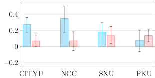
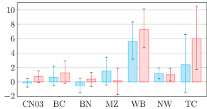
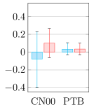
Fig. 2 illustrates the relative improvement achieved by two larger-context methods: seq (blue bar) and cPre-seq (red bar) on four different tagging tasks. We observe that:

1) In general, aggregators equipped with BERT can not guarantee a better improvement, which is dataset-dependent. 2) Task-wisely, cPre-seq can improve performance on all datasets on NER, Chunk, and POS tasks. By contrast, seq is beneficial to all datasets on CWS task. It could be attributed to the difference in language and characteristics of the task. Specifically, for most non-CWS task datasets, cPre-seq (7 out of 9 datasets) performs better than seq ($p<0.05$).

5 Experiment: Why Does It Work?

Experiments in this section are designed for the research questions Q3, interpreting where the gains of a larger-context approach come and why different datasets exhibit diverse improvements. To achieve this goal, we use the concept of interpretable evaluation Fu et al. (2020a) that allows us perform fine-grained evaluation of one or multiple systems.

5.1 Attribute Definition

The first step of interpretable evaluation is attribute definition. The high-level idea is, given one attribute, the test set of each tagging task will be partitioned into several interpretable buckets based on it. And $F$1 score (accuracy for POS) will be calculated bucket-wisely. Next, we will explicate the general attributes we defined in this paper.

We first detail some notations to facilitate definitions of our attributes. We define $x$ as a token and a bold form $\mathbf{x}$ as a span, which occurs in a test sentence $X=\mathrm{sent}(\mathbf{x})$. We additionally define two functions $\mathrm{oov(\cdot)}$ that counts the number out of training set words, and $\mathrm{ent(\cdot)}$ that tallies the number of entity words. Based on these notations, we introduce some feature functions that can compute different attributes for each span or token. Following, we will give the attribute definition of the NER.

Training set-independent Attributes

• $\phi_{\texttt{eLen}}(\mathbf{x})=|\mathbf{x}|$: entity span length

• $\phi_{\texttt{sLen}}(\mathbf{x})=|\mathrm{sent}(\mathbf{x})|$: sentence length

• $\phi_{\texttt{eDen}}(\mathbf{x})=|\mathrm{ent}(sent(\mathbf{x}))|/\phi_{\texttt{sLen}}(\mathbf{x})$: entity density

• $\phi_{\texttt{dOov}}(\mathbf{x})=|\mathrm{oov}(\mathrm{sent}(\mathbf{x}))|/\phi_{\texttt{sLen}}(\mathbf{x})$: OOV density

Training set-dependent Attributes

• $\phi_{\texttt{eFre}}(\mathbf{x})=\mathrm{Fre}(\mathbf{x})$: entity frequency

• $\phi_{\texttt{eCon}}(\mathbf{x})=\mathrm{Con}(\mathbf{x})$: label consistency of entity

where $\mathrm{Fre}(\mathbf{x})$ calculates the frequency of input $\mathbf{x}$ in the training set. $\mathrm{Con}(\mathbf{x})$ quantify how consistently a given span is labeled with a particular label, and $\mathrm{Con}(\mathbf{x})$ can be formulated as:

$$\mathrm{Con}(\mathbf{x}) =\frac{|\{\varepsilon|\mathrm{lab}(\varepsilon)(\mathbf{x}),\forall\varepsilon\in\mathcal{E}^{tr}\}|}{|\mathrm{str}(\varepsilon)=\mathrm{str}(\mathbf{x}),\forall\varepsilon\in\mathcal{E}^{tr}\}|},$$ (10)

$$\mathrm{lab}(\varepsilon) =\mathrm{lab}(\mathbf{x})\cap\mathrm{str}(\varepsilon)=\mathrm{str}(\mathbf{x}),$$ (11)

where $\mathcal{E}^{tr}$ denotes entities in the training set, $\mathrm{lab}(\cdot)$ denotes the label of input span while $\mathrm{str}(\cdot)$ represents the surface string of input span. Similarly, we can extend the above two attributes to token-level, therefore obtaining $\phi_{\texttt{tFre}}(x)$ and $\phi_{\texttt{tCon}}(x)$.

Attributes for CWS task can be defined in a similar way. Specifically, the entity (or token) in NER task corresponds to the word (or character) in CWS task. Note that we omit word density for CWS task since it equals to one for any sentence.

5.2 Attribute Buckets

We breakdown all test examples into different attribute buckets according to the given attribute. Take entity length (eLen) attribute of NER task as an example, first, we calculate each test sample’s entity length attribute value. Then, divide the test entities into $N$ attribute buckets ($N=4$ by default) where the numbers of the test samples in all attribute intervals (buckets) are equal, and calculate the performance for those entities falling into the same bucket.

5.3 Exp-I: Breakdown over Attributes

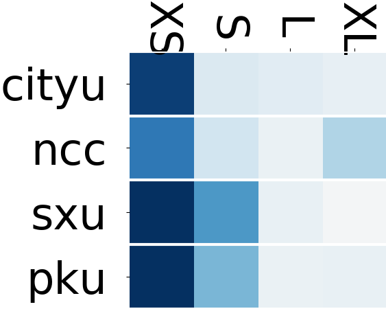
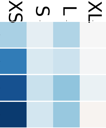
To investigate where the gains of the larger-context training come, we conduct a fine-grained evaluation with the evaluation attributes defined in Sec. 5.1. We use the cPre-seq larger-context aggregation method as the base model. Fig. 3 shows the relative improvement of the cPre-seq larger-context aggregation method in NER ($7$ datasets) and CWS tasks ($4$ datasets). The relative improvement is the performance of cPre-seq larger-context tagging minus sentence-level tagging.

Results

Our findings from Fig. 3 are:

1) Test spans with lower label consistency can benefit much more from the larger-context training. As shown in Fig. 3 (a,b,i,j), test spans with lower label consistency (NER:eCon,tCon=S/XS, CWS: wCon,cCon=S/XS) can achieve higher relative improvement using the larger-context training, which holds for both NER and CWS tasks.

2) NER task has achieved more gains on lower and higher-frequency test spans, while CWS task obtains more gains on lower-frequency test spans. As shown in Fig. 2 (c,d,k,l), in NER task, test spans with higher or lower frequency (NER:eFre=XS/XL;tFre=XS/XL) will achieve larger improvements with the help of more contextual sentences; while for the CWS task, only the test spans with lower frequency will achieve more gains.

(a) eCon

(b) tCon

(c) eFre

(d) tFre

(e) eDen

(f) eLen

(g) sLen

(h) dOov

(i) wCon

(j) cCon

(k) wFre

(l) cFre

(m) wLen

(n) sLen

(o) dOov

Figure 3: The relative increase ($\in[0,1]$) of the cPre-seq larger-context training on NER (a$-$h) and CWS (i$-$o) tasks based on their evaluation attributes. “co” denotes the CoNLL-2003 dataset. In order to facilitate observation, we divide the attribute value range into four categories: extra-small (XS), small (S), large (L), and extra-large (XL). The darker blue implies more significant improvement while the darker red suggests larger-context leads to worse performance. For the attribute name, “e”, “t”, “w”, and “c” refers to “entity”, “token”, “word”, and “character”, respectively.

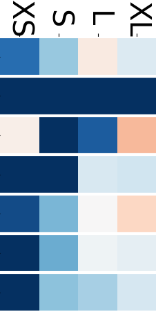
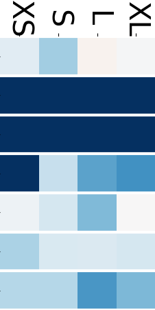
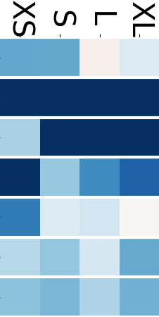
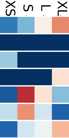
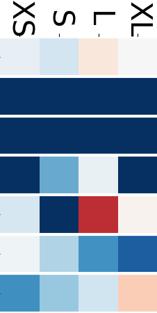
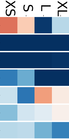
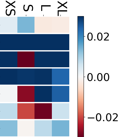
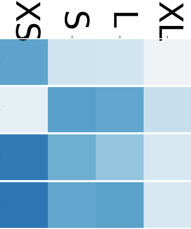
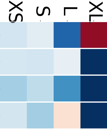
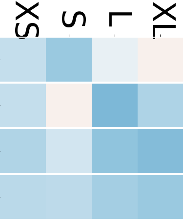
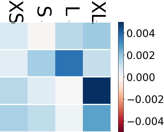
3) Test spans of NER task with lower entity density have obtained larger improvement with the help of a larger-context training. In terms of entity density shown in Fig. 3 (e), an evaluation attribute specific to the NER task, the larger-context training is not good at dealing with the test spans with high entity density (NER:eDen=XL/L), while doing well in test spans with low entity density (NER:eDen=XS/S).

4) Larger-context training can achieve more gains on short entities in NER task while long words in CWS task. As shown in Fig. 3 (f,m), the dark blue boxes can be seen in the short entities (eLen=XS/S) of NER task, and long words (wLen=XL/L) of CWS task.

5) Both NER and CWS tasks will achieve more gains on spans with higher OOV density. For the OOV density shown in Fig. 2 (h,o), the test spans with higher OOV density (NER,CWS:dOov=L/XL) will achieve more gains from the larger-context training, which holds for both NER and CWS tasks.

	Attr.	eCon	tCon	eFre	tFre	eLen	dOov	sLen	eDen
$\zeta_{p}$
$\rho$	bow	-0.179	-0.607	0.143	0.396	0.643	-0.036	0.468	-0.571
	graph	-0.571	-0.143	-0.393	-0.919	-0.643	0.286	-0.288	-0.107
	seq	-0.643	-0.857	-0.429	0.162	0.143	0.071	0.180	-0.714
	cPre	-0.714	-0.750	-0.571	-0.306	0.000	0.357	-0.180	-0.643

Table 2: Illustration of measures $\zeta_{p}$ in seven datasets (CN03, TC, NW, WB, MZ, BN, BC) with respect to eight attributes (e.g., eCon) and correlation measure $\rho$ in NER task. A higher absolute value $\rho$ (e.g |-0.714|) represents the improvement of the corresponding aggregator (e.g., seq) heavily correlates with corresponding attribute (e.g. eCon). The number with the highest absolute value of each column is colored by green. “cPre” represents “cPre-seq” and the values in grey denote correlation values do not pass a significance test ($p=0.05$). “Attr.” denotes attributes.

5.4 Exp-II: Quantifying and Understanding Dataset Bias

Different datasets (e.g. CN03) may match different information aggregators (e.g. cPre-seq). Figuring out how different datasets influence the choices of aggregators is a challenging task. We try to approach this goal by (i) designing diverse measures that can characterize a given dataset from different perspectives, (ii) analyzing the correlation between different dataset properties and improvements brought by different aggregators.

Dataset-level Measure

Given a dataset $\mathcal{E}$ and an attribute $p$ as defined in Sec. 5.1, the data-level measure can be defined as:

$$\zeta_{p}(\mathcal{E})=\frac{1}{|\mathcal{E}^{te}|}\sum_{\varepsilon\in\mathcal{E}^{te}}\phi_{p}(\varepsilon),$$ (12)

where $\mathcal{E}^{te}\in\mathcal{E}$ is a test set that contains entities/tokens in the NER task or word/character in the CWS task. $\phi_{p}(\cdot)$ is a function (as defined in Sec. 5.1) that computes the attribute value for a given span. For example, $\zeta_{\texttt{sLen}}(\texttt{CN03})$ represents the average sentence length of CN03’s test set.

Correlation Measure

Statistically, we define a variable of $\rho$ to quantify the correlation between a dataset-level attribute and the relative improvement of an aggregator: $\rho=\mathrm{Spearman}(\zeta_{p},f_{y})$, where $\mathrm{Spearman}$ denotes the Spearman’s rank correlation coefficient Mukaka (2012). $\zeta_{p}$ represents dataset-level attribute values on all datasets with respect to attribute $p$ (e.g., eLen) while $f_{y}$ denotes the relative improvements of larger-context training on corresponding datasets with respect to a given aggregator $y$ (e.g., cPre-seq).

Results

Tab. 2 displays (using spider charts) measure $\zeta_{p}$  of seven datasets with respect to diverse attributes, and correlation measure $\rho$ in the NER task.  Based on these correlations, which passed significantly test ($p<0.05$), between dataset-level measure (w.r.t a certain attribute, e.g. eCon) and gains from larger-context training (w.r.t an aggregator, e.g. seq), we can obtain that:

(1) Regarding the cPre-seq aggregator, it negatively correlated with $\zeta_{\texttt{eCon}}$, $\zeta_{\texttt{tCon}}$, $\zeta_{\texttt{eFre}}$, and $\zeta_{\texttt{eDen}}$ with larger correlation values. Therefore, the cPre-seq aggregator is more appropriate to deal with WB, TC, BC and NW datasets, since these four datasets have a lower value of $\zeta_{p}$ with respect to the attribute eCon (TC,WB), tCon (TC, WB), eFre (NW, TC), and eDen (BC, WB, TC). Additionally, since the cPre-seq aggregator obtains the highest positive correlation with $\zeta_{\texttt{dOov}}$, and $\zeta_{\texttt{dOov}}(\texttt{CN03})$, as well as $\zeta_{\texttt{dOov}}(\texttt{BC})$, achieve the highest value, cPre-seq aggregator is suitable for CN03 and BC.

(2) Regarding the seq aggregator, it negatively correlated with $\zeta_{\texttt{eCon}}$, $\zeta_{\texttt{tCon}}$, and $\zeta_{\texttt{eDen}}$. Therefore, the seq aggregator is better at dealing with datasets WB, TC, and BC, since these datasets are with lower $\zeta_{p}$ value on one of the attributes (eCon, tCon, and eDen).

Takeaways:

We can conduct a similar analysis for bow and graph aggregators. Due to limited pages, we detail them in our appendix and highlight the suitable NER datasets for each aggregator as follows.

• bow: WB, TC, NW, MZ, BC.

• graph: WB, TC, BN, CN03.

• seq: WB, TC, BC.

• cPre-seq: CN03, WB, TC, BC, NW.

6 Adapting to Top-Scoring Systems

Beyond the above quantitative and qualitative analysis of our instantiated typical tagging models (Sec.2.3), we are also curious about how well modern top-scoring tagging systems perform when equipped with larger-context training.

To this end, we choose the NER task as a case study and first re-implement existing top-performing models for different NER datasets separately, and then adapt larger-context approach to them based on the seq or cPre-seq aggregator, which has shown superior performance in our above analysis.

Settings

We collect five top-scoring tagging systems Luo et al. (2020); Lin et al. (2019); Chen et al. (2019); Yan et al. (2019); Akbik et al. (2018) that are most recently proposed . Among these five models, regarding Akbik et al. (2018), we use cPre-seq aggregator for the larger-context training, since this model originally relies on a contextualized pre-trained layer. Besides, from above analysis in Sec. 5.4 we know the suitable datasets for cPre-seq aggregator: CN03, WB, TC, BC, and NW. Regarding the other four models, we use the seq aggregator for the larger-context training and the matched datasets are: WB, TC, and BC.

Results

Tab. 3 shows the relative improvement of larger-context training on five modern top-scoring models in the NER task. We observe that the larger-context training has achieved consistent gains on all chosen datasets, which holds for both seq and cPre-seq aggregators. Notably, the larger-cotext training achieves sharp improvement on WB, which holds for all the five top-scoring models. For example, with the help of larger-context training, the performance can be improved significantly using Akbik et al. (2018) and 7.18 $F1$ score using Luo et al. (2020). This suggests that modern top-scoring NER systems can also benefit from larger-context training.

Models	Aggregator			Datasets
	norm	seq	cPre	BC	WB	TC	CN03	NW
Luo et al. (2020)	$\surd$			78.78	62.38	65.56	-	-
		$\surd$		+0.54	+7.18	+1.7
Lin et al. (2019)	$\surd$			77.80	63.16	65.19	-	-
		$\surd$		+2.94	+5.07	+2.25
Chen et al. (2019)	$\surd$			77.50	66.51	65.49	-	-
		$\surd$		+1.96	+3.98	+0.89	-	-
Yan et al. (2019)	$\surd$			81.29	65.05	67.92	92.17	90.37
		$\surd$		+0.16	+6.79	+3.03	+0.04	+1.11
Akbik et al. (2018)	$\surd$			81.13	64.79	69.00	93.03	90.76
			$\surd$	+1.12	+10.78	+2.12	+0.05	+1.03

Table 3: The relative improvement of larger-context training on top-scoring models in the NER task.  “cPre” represents “cPre-seq”. “norm” denotes the normal setting ($K=1$). The testing datasets are chosen based on the analysis in Sec. 5.4.

7 Related Work

Our work touches the following research topics for tagging tasks.

Sentence-level Tagging Existing works have achieved impressive performance at sentence-level tagging by extensive structural explorations with different types of neural components. Regarding sentence encoders, recurrent neural nets Huang et al. (2015); Chiu and Nichols (2015); Ma and Hovy (2016); Lample et al. (2016); Li et al. (2019); Lin et al. (2020) and convolutional neural nets Strubell et al. (2017); Yang et al. (2018); Chen et al. (2019); Fu et al. (2020a) were widely used while transformer were also studied to get sentential representations Yan et al. (2019); Yu et al. (2020). Some recent works consider the NER as a span classification Li et al. (2019); Jiang et al. (2019); Mengge et al. (2020); Ouchi et al. (2020) task, unlike most works that view it as a sequence labeling task. To capture morphological information, some previous works introduced a character or subword-aware encoders with unsupervised pre-trained knowledge  Peters et al. (2018); Akbik et al. (2018); Devlin et al. (2018); Akbik et al. (2019); Yang et al. (2019); Lan et al. (2019).

Document-level Tagging Document-level tagging introduced more contextual features to improve the performance of tagging. Some early works introduced non-local information Finkel et al. (2005); Krishnan and Manning (2006) to enhance traditional machine learning methods (e.g., CRF Lafferty et al. (2001)) and achieved impressive results. Qian et al. (2018); Wadden et al. (2019) built graph representation based on the broad dependencies between words and sentences. Luo et al. (2020) proposed to use a memory network to record the document-aware information. Besides, document-level features was introduced by different domains to alleviate label inconsistency problems, such as news NER Hu et al. (2020, 2019), chemical NER Luo et al. (2018), disease NER Xu et al. (2019), and Chinese patent Li and Xue (2014, 2016). Compared with these works, instead of proposing a novel model, we focus on investigating when and why the larger-context training, as a general strategy, can work.

Interpretability and Robustness of Sequence Labeling Systems

Recently, there is a popular trend that aims to (i) perform a glass-box analysis of sequence labeling systems Fu et al. (2020b); Agarwal et al. (2020), understanding their generalization ability and quantify robustness Fu et al. (2020c), (ii) interpretable evaluation of them Fu et al. (2020a), making it possible to know what a system is good/bad at and where a system outperforms another, (iii) reliable analysis Ye et al. (2021) for test set with fewer samples. Our work is based on the technique of interpretable evaluation, which provides a convenient way for us to diagnose different systems.

8 Discussion

We summarize the main observations from our experiments and try to provide preliminary answers to our proposed research questions:

(i) How do different integration ways of larger-context information influence the system’s performance? Overall, introducing larger-context information will bring gains regardless of the ways how to introduce it (e.g., seq, graph). Particularly, larger-context training with seq aggregator can achieve better performance at lower training cost compared with graph and bow aggregators (Sec. 4.1).

(ii) Can the larger-context training easily play to its strengths with the help of contextualized pre-trained models? Yes for all datasets on NER, Chunk, and POS tasks. By contrast, for CWS tasks, the aggregator without BERT (e.g., seq) can achieve better improvement (Sec. 4.2).

(iii) Where does the gain of larger-context training come? And how do different characteristics of datasets affect the amount of gain? The source of gains, though, is dataset- and aggregator-dependent, a relatively consensus observation is that text spans with lower label consistency and higher OOV density can benefit a lot from larger-context training (Sec. 5.3). Regarding different datasets, diverse aggregators are recommended in Sec. 5.4.

Agg.	CITYU	NCC	SXU	PKU	CN03	BC	BN	MZ	WB	NW	TC	CN00	PTB
bow	5	6	2	2	2	5	4	2	10	2	5	2	4
graph	7	3	3	6	10	6	4	3	7	6	10	3	10
seq	7	3	3	6	10	6	4	3	7	6	10	3	10
cPre	7	3	3	6	10	7	4	3	7	6	10	2	10

Table 4: The window size $k$ when the four larger-context aggregators achieve the final performance.

Task	Data	eCon	tCon	eFre	tFre	eLen	dOov	sLen	eDen
NER	CN03	0.485	0.514	0.109	0.017	1.436	0.067	13.4	0.232
	BC	0.486	0.440	0.113	0.108	1.905	0.064	16.3	0.085
	BN	0.627	0.552	0.147	0.089	1.623	0.004	19.5	0.148
	MZ	0.496	0.487	0.129	0.119	1.832	0.015	22.9	0.124
	WB	0.294	0.269	0.111	0.084	1.631	0.024	22.9	0.050
	NW	0.567	0.512	0.083	0.108	2.015	0.014	26.1	0.179
	TC	0.261	0.258	0.082	0.105	1.598	0.043	8.3	0.040
Task	Data	wCon	cCon	wFre	cFre	wLen	dOov	sLen
CWS	CITYU	0.763	0.285	1.834	0.489	1.634	0.010	62.400
	NCC	0.743	0.274	3.856	1.016	1.546	0.021	64.400
	SXU	0.781	0.293	3.832	1.005	1.590	0.020	69.700
	PKU	0.777	0.292	1.765	0.466	1.615	0.019	59.200

Table 5: The data-level measure $\zeta_{p}$ in seven (four) datasets with respect to eight (seven) attributes in NER (CWS) task. The value of wFre and cFre on CWS task needs to multiply by $10^{-7}$.

Appendix A Aggregator Setting

Tab. 4 illustrates the window size $k(k\neq 1)$ when the larger-context aggregator achieves the best performance. The window size $k$ when seq achieves the best performance will be chosen to set the document-length of the graph aggregator.

	Attr.	eCon	tCon	eFre	tFre	eLen	dOov	sLen	eDen
$\zeta_{p}$
$\rho$	bow	-0.179	-0.607	0.143	0.396	0.643	-0.036	0.468	-0.571
	graph	-0.571	-0.143	-0.393	-0.919	-0.643	0.286	-0.288	-0.107
	seq	-0.643	-0.857	-0.429	0.162	0.143	0.071	0.180	-0.714
	cPre	-0.714	-0.750	-0.571	-0.306	0.000	0.357	-0.180	-0.643

Table 6: Illustration of measures $\zeta_{p}$ in seven datasets (CN03, TC, NW, WB, MZ, BN, BC) with respect to eight attributes (e.g., eCon) and correlation measure $\rho$ in NER task. A higher absolute value $\rho$ (e.g |-0.714|) represents the improvement of corresponding aggregator (e.g., seq) heavily correlate with corresponding attribute (e.g. eCon). The number with the highest absolute value of each column is colored by green. “cPre” represents “cPre-seq” and the value in grey denotes correlation value does not pass a significance test ($p=0.05$).

Appendix B Quantifying and Understanding Dataset Bias

In this section, we will supplement some analyses related to Sec. 5.3.

B.1 Data-level Measure

Tab. 5 gives the data-level measure $\zeta_{p}$ in seven (four) datasets with respect to eight (seven) attributes in NER (CWS) task. The data-level measure $\zeta_{p}$ will be used to compute the correlation measure in Sec. 5.3.

B.2 Results

Tab. 6 displays (using spider charts) measure $\zeta_{p}$ of seven datasets with respect to diverse attributes, and correlation measure $\rho$ in NER task. We have given a detail analysis on seq and cPre-seq on the main text, here, we will provide the suggestion for choosing the datasets for bow and graph aggregator.

(1) regarding bow aggregator, it negatively correlated with $\zeta_{\texttt{tCon}}$ and $\zeta_{\texttt{eDen}}$ with larger correlation values. Therefore, bow aggregator is more appropriate to deal with datasets WB, TC, BC, since these four datasets are with lower value of $\zeta_{p}$ with respect to the attribute tCon (TC, WB) and eDen (BC, WB, TC). Additionally, bow aggregator obtained the highest positive correlation with $\zeta_{\texttt{tFre}}$, $\zeta_{\texttt{eLen}}$, and $\zeta_{\texttt{sLen}}$. Besides, $\zeta_{\texttt{tFre}}(\texttt{MZ})$, $\zeta_{\texttt{eLen}}(\texttt{NW})$, and $\zeta_{\texttt{sLen}}(\texttt{NW})$, also achieved the highest value, suggesting that bow aggregator is suitable for MZ and NW.

(2) regarding graph aggregator, it negatively correlated with $\zeta_{\texttt{eCon}}$, $\zeta_{\texttt{eFre}}$, $\zeta_{\texttt{tFre}}$, and $\zeta_{\texttt{eLen}}$, with larger correlation values. Therefore, graph aggregator is more appropriate to deal with datasets WB, TC, NW, and CN03, since these four datasets are with lower value of $\zeta_{p}$ with respect to the attribute eCon (TC,WB), eFre (NW, TC), tFre (CN03, WB), and eLen (CN03),.

	Attr.	wCon	cCon	wFre	cFre	wLen	dOov	sLen
$\zeta_{p}$
$\rho$	bow	-0.657	-0.771	0.086	0.257	-0.600	0.319	-0.486
	graph	-0.029	0.257	-0.543	-0.429	0.143	-0.319	-0.486
	seq	0.086	-0.200	0.371	0.314	-0.257	0.464	0.257
	cPre	0.580	0.493	-0.261	-0.203	-0.203	0.544	-0.232

Table 7: Illustration of measures $\zeta_{p}$ in four datasets ( CITYU, NCC, SXU, PKU) with respect to seven attributes (e.g., wCon) and correlation measure $\rho$ in CWS task. A higher absolute value $\rho$ (e.g |-0.657|) represents the improvement of corresponding aggregator (e.g., bow) heavily correlate with corresponding attribute (e.g. wCon). The number with the highest absolute value of each column is colored by green. “cPre” represents “cPre-seq” and the value in grey denotes correlation value does not pass a significance test ($p=0.05$).

Tab. 7 illustrates the measures $\zeta_{p}$ in four CWS datasets with respect to seven attributes (e.g., wCon) and correlation measure $\rho$. We can conduct similar analysis like NER for CWS. We highlight the suitable CWS datasets for each aggregator as follows:

• bow: NCC, and SXU.

• graph: PKU and CITYU.

• seq: SXU, and NCC.

• cPre-seq: CITYU, PKU, SXU.

References

- Agarwal et al. (2020) Oshin Agarwal, Yinfei Yang, Byron C Wallace, and Ani Nenkova. 2020. Interpretability analysis for named entity recognition to understand system predictions and how they can improve. arXiv preprint arXiv:2004.04564.
- Akbik et al. (2019) Alan Akbik, Tanja Bergmann, and Roland Vollgraf. 2019. Pooled contextualized embeddings for named entity recognition. pages 724–728.
- Akbik et al. (2018) Alan Akbik, Duncan Blythe, and Roland Vollgraf. 2018. Contextual string embeddings for sequence labeling. In Proceedings of the 27th International Conference on Computational Linguistics, pages 1638–1649.
- Chen et al. (2019) Hui Chen, Zijia Lin, Guiguang Ding, Jianguang Lou, Yusen Zhang, and Borje Karlsson. 2019. Grn: Gated relation network to enhance convolutional neural network for named entity recognition. In Proceedings of the AAAI Conference on Artificial Intelligence, volume 33, pages 6236–6243.
- Chiu and Nichols (2015) Jason P C Chiu and Eric Nichols. 2015. Named entity recognition with bidirectional lstm-cnns. arXiv: Computation and Language.
- Chiu and Nichols (2016) Jason PC Chiu and Eric Nichols. 2016. Named entity recognition with bidirectional lstm-cnns. Transactions of the Association for Computational Linguistics, 4:357–370.
- Devlin et al. (2018) Jacob Devlin, Ming-Wei Chang, Kenton Lee, and Kristina Toutanova. 2018. Bert: Pre-training of deep bidirectional transformers for language understanding. arXiv preprint arXiv:1810.04805.
- Durrett and Klein (2014) Greg Durrett and Dan Klein. 2014. A joint model for entity analysis: Coreference, typing, and linking. Transactions of the association for computational linguistics, 2:477–490.
- Efron and Tibshirani (1986) Bradley Efron and Robert Tibshirani. 1986. Bootstrap methods for standard errors, confidence intervals, and other measures of statistical accuracy. Statistical science, pages 54–75.
- Finkel et al. (2005) Jenny Rose Finkel, Trond Grenager, and Christopher Manning. 2005. Incorporating non-local information into information extraction systems by gibbs sampling. In Proceedings of the 43rd annual meeting on association for computational linguistics, pages 363–370. Association for Computational Linguistics.
- Fu et al. (2020a) Jinlan Fu, Pengfei Liu, and Graham Neubig. 2020a. Interpretable multi-dataset evaluation for named entity recognition. In Proceedings of the 2020 Conference on Empirical Methods in Natural Language Processing (EMNLP), pages 6058–6069, Online. Association for Computational Linguistics.
- Fu et al. (2020b) Jinlan Fu, Pengfei Liu, and Qi Zhang. 2020b. Rethinking generalization of neural models: A named entity recognition case study. In Proceedings of the AAAI Conference on Artificial Intelligence, volume 34, pages 7732–7739.
- Fu et al. (2020c) Jinlan Fu, Pengfei Liu, Qi Zhang, and Xuanjing Huang. 2020c. RethinkCWS: Is Chinese word segmentation a solved task? In Proceedings of the 2020 Conference on Empirical Methods in Natural Language Processing (EMNLP), pages 5676–5686, Online. Association for Computational Linguistics.
- Ghaddar and Langlais (2018) Abbas Ghaddar and Philippe Langlais. 2018. Robust lexical features for improved neural network named-entity recognition. arXiv preprint arXiv:1806.03489.
- Hu et al. (2019) Anwen Hu, Zhicheng Dou, and Ji-rong Wen. 2019. Document-level named entity recognition by incorporating global and neighbor features. In China Conference on Information Retrieval, pages 79–91. Springer.
- Hu et al. (2020) Anwen Hu, Zhicheng Dou, Jirong Wen, and Jianyun Nie. 2020. Leveraging multi-token entities in document-level named entity recognition.
- Huang et al. (2015) Zhiheng Huang, Wei Xu, and Kai Yu. 2015. Bidirectional lstm-crf models for sequence tagging. arXiv: Computation and Language.
- Jiang et al. (2019) Zhengbao Jiang, Wei Xu, Jun Araki, and Graham Neubig. 2019. Generalizing natural language analysis through span-relation representations. arXiv preprint arXiv:1911.03822.
- Kipf and Welling (2016) Thomas N Kipf and Max Welling. 2016. Semi-supervised classification with graph convolutional networks. arXiv preprint arXiv:1609.02907.
- Krishnan and Manning (2006) Vijay Krishnan and Christopher D Manning. 2006. An effective two-stage model for exploiting non-local dependencies in named entity recognition. In Proceedings of the 21st International Conference on Computational Linguistics and the 44th annual meeting of the Association for Computational Linguistics, pages 1121–1128. Association for Computational Linguistics.
- Lafferty et al. (2001) John D. Lafferty, Andrew McCallum, and Fernando C. N. Pereira. 2001. Conditional random fields: Probabilistic models for segmenting and labeling sequence data. In Proceedings of the Eighteenth International Conference on Machine Learning.
- Lample et al. (2016) Guillaume Lample, Miguel Ballesteros, Sandeep Subramanian, Kazuya Kawakami, and Chris Dyer. 2016. Neural architectures for named entity recognition. In Proceedings of NAACL-HLT, pages 260–270.
- Lan et al. (2019) Zhenzhong Lan, Mingda Chen, Sebastian Goodman, Kevin Gimpel, Piyush Sharma, and Radu Soricut. 2019. Albert: A lite bert for self-supervised learning of language representations. arXiv preprint arXiv:1909.11942.
- Li and Xue (2014) Si Li and Nianwen Xue. 2014. Effective document-level features for chinese patent word segmentation. 2:199–205.
- Li and Xue (2016) Si Li and Nianwen Xue. 2016. Towards accurate word segmentation for chinese patents. arXiv: Computation and Language.
- Li et al. (2019) Xiaoya Li, Jingrong Feng, Yuxian Meng, Qinghong Han, Fei Wu, and Jiwei Li. 2019. A unified mrc framework for named entity recognition. arXiv preprint arXiv:1910.11476.
- Lin et al. (2020) Bill Yuchen Lin, Dong-Ho Lee, Ming Shen, Ryan Moreno, Xiao Huang, Prashant Shiralkar, and Xiang Ren. 2020. Triggerner: Learning with entity triggers as explanations for named entity recognition. arXiv preprint arXiv:2004.07493.
- Lin et al. (2019) Ying Lin, Liyuan Liu, Heng Ji, Dong Yu, and Jiawei Han. 2019. Reliability-aware dynamic feature composition for name tagging. In Proceedings of the 57th Annual Meeting of the Association for Computational Linguistics, pages 165–174.
- Luo et al. (2018) Ling Luo, Zhihao Yang, Pei Yang, Yin Zhang, Lei Wang, Hongfei Lin, and Jian Wang. 2018. An attention-based bilstm-crf approach to document-level chemical named entity recognition. Bioinformatics, 34(8):1381–1388.
- Luo et al. (2020) Ying Luo, Fengshun Xiao, and Hai Zhao. 2020. Hierarchical contextualized representation for named entity recognition.
- Ma and Hovy (2016) Xuezhe Ma and Eduard Hovy. 2016. End-to-end sequence labeling via bi-directional lstm-cnns-crf. In Proceedings of the 54th Annual Meeting of ACL, volume 1, pages 1064–1074.
- Mengge et al. (2020) Xue Mengge, Bowen Yu, Zhenyu Zhang, Tingwen Liu, Yue Zhang, and Bin Wang. 2020. Coarse-to-fine pre-training for named entity recognition. In Proceedings of the 2020 Conference on Empirical Methods in Natural Language Processing (EMNLP), pages 6345–6354.
- Mikolov et al. (2013) Tomas Mikolov, Ilya Sutskever, Kai Chen, Greg S Corrado, and Jeff Dean. 2013. Distributed representations of words and phrases and their compositionality. In Advances in neural information processing systems, pages 3111–3119.
- Mukaka (2012) Mavuto Mukaka. 2012. Statistics corner: A guide to appropriate use of correlation coefficient in medical research. Malawi medical journal : the journal of Medical Association of Malawi, 24(3):69–71.
- Ouchi et al. (2020) Hiroki Ouchi, Jun Suzuki, Sosuke Kobayashi, Sho Yokoi, Tatsuki Kuribayashi, Ryuto Konno, and Kentaro Inui. 2020. Instance-based learning of span representations: A case study through named entity recognition. arXiv preprint arXiv:2004.14514.
- Pennington et al. (2014) Jeffrey Pennington, Richard Socher, and Christopher D Manning. 2014. Glove: Global vectors for word representation. Proceedings of the EMNLP, 12:1532–1543.
- Peters et al. (2018) Matthew Peters, Mark Neumann, Mohit Iyyer, Matt Gardner, Christopher Clark, Kenton Lee, and Luke Zettlemoyer. 2018. Deep contextualized word representations. In Proceedings of the 2018 Conference of the North American Chapter of the Association for Computational Linguistics: Human Language Technologies, Volume 1 (Long Papers), volume 1, pages 2227–2237.
- Pineau et al. (2020) Joelle Pineau, Philippe Vincent-Lamarre, Koustuv Sinha, Vincent Larivière, Alina Beygelzimer, Florence d’Alché Buc, Emily Fox, and Hugo Larochelle. 2020. Improving reproducibility in machine learning research (a report from the neurips 2019 reproducibility program). arXiv preprint arXiv:2003.12206.
- Qian et al. (2018) Yujie Qian, Enrico Santus, Zhijing Jin, Jiang Guo, and Regina Barzilay. 2018. Graphie: A graph-based framework for information extraction. arXiv: Computation and Language.
- Sang and De Meulder (2003) Erik F Sang and Fien De Meulder. 2003. Introduction to the conll-2003 shared task: Language-independent named entity recognition. arXiv preprint cs/0306050.
- Schlichtkrull et al. (2018) Michael Schlichtkrull, Thomas N Kipf, Peter Bloem, Rianne Van Den Berg, Ivan Titov, and Max Welling. 2018. Modeling relational data with graph convolutional networks. In European Semantic Web Conference, pages 593–607. Springer.
- Strubell et al. (2017) Emma Strubell, Patrick Verga, David Belanger, and Andrew Mccallum. 2017. Fast and accurate entity recognition with iterated dilated convolutions. pages 2670–2680.
- Wadden et al. (2019) David Wadden, Ulme Wennberg, Yi Luan, and Hannaneh Hajishirzi. 2019. Entity, relation, and event extraction with contextualized span representations. arXiv preprint arXiv:1909.03546.
- Wilcoxon et al. (1970) Frank Wilcoxon, SK Katti, and Roberta A Wilcox. 1970. Critical values and probability levels for the wilcoxon rank sum test and the wilcoxon signed rank test. Selected tables in mathematical statistics, 1:171–259.
- Xu et al. (2019) Kai Xu, Zhenguo Yang, Peipei Kang, Qi Wang, and Wenyin Liu. 2019. Document-level attention-based bilstm-crf incorporating disease dictionary for disease named entity recognition. Computers in biology and medicine, 108:122–132.
- Yan et al. (2019) Hang Yan, Bocao Deng, Xiaonan Li, and Xipeng Qiu. 2019. Tener: Adapting transformer encoder for name entity recognition. arXiv preprint arXiv:1911.04474.
- Yang et al. (2018) Jie Yang, Shuailong Liang, and Yue Zhang. 2018. Design challenges and misconceptions in neural sequence labeling. arXiv: Computation and Language.
- Yang et al. (2019) Zhilin Yang, Zihang Dai, Yiming Yang, Jaime Carbonell, Russ R Salakhutdinov, and Quoc V Le. 2019. Xlnet: Generalized autoregressive pretraining for language understanding. In Advances in neural information processing systems, pages 5753–5763.
- Ye et al. (2021) Zihuiwen Ye, Pengfei Liu, Jinlan Fu, and Graham Neubig. 2021. Towards more fine-grained and reliable nlp performance prediction. arXiv preprint arXiv:2102.05486.
- Yu et al. (2020) Jianfei Yu, Jing Jiang, Li Yang, and Rui Xia. 2020. Improving multimodal named entity recognition via entity span detection with unified multimodal transformer. Association for Computational Linguistics.