Right Handed Neutrinos, TeV Scale BSM Neutral Higgs and FIMP Dark Matter in EFT Framework

Abstract

We consider an effective field theory framework with three standard model (SM) gauge singlet right handed neutrinos, and an additional SM gauge singlet scalar field. The framework successfully generates eV masses of the light neutrinos via seesaw mechanism, and accommodates a feebly interacting massive particle (FIMP) as dark matter candidate. Two of the gauge singlet neutrinos participate in neutrino mass generation, while the third gauge singlet neutrino is a FIMP dark matter. We explore the correlation between the vev of the gauge singlet scalar field which translates as mass of the BSM Higgs, and the mass of dark matter, which arises due to relic density constraint. We furthermore explore the constraints from the light neutrino masses in this set-up. We chose the gauge singlet BSM Higgs in this framework in the TeV scale. We perform a detailed collider analysis to analyse the discovery prospect of the TeV scale BSM Higgs through its di-fatjet signature, at a future $pp$ collider which can operate with $\sqrt{s}=100$ TeV c.m.energy.

1 Introduction

The Standard Model (SM) of particle physics, despite its accurate predictions suffers from few serious deficits. Two of the most serious drawbacks emerge from the observation of light neutrino masses and their mixings, and the precise measurement of dark matter (DM) relic abundance in the Universe. A number of neutrino oscillation experiments have confirmed that the solar and atmospheric neutrino mass splittings are $\Delta m^{2}_{21}\sim 10^{-5}\,\rm{eV}^{2}$, $|\Delta m^{2}_{13}|\sim 10^{-3}\,\rm{eV}^{2}$, the Pontecorvo-Maki-Nakagawa-Sakata (PMNS) mixing angles Maki:1962mu ; Pontecorvo:1967fh are $\theta_{12}\sim 33^{\circ}$, $\theta_{23}\sim 49^{\circ}$, and $\theta_{13}\sim 8^{\circ}$ Esteban:2020cvm . The light neutrinos being electromagnetic charge neutral can be Majorana particles. One of the profound mechanisms to generate Majorana masses of the light neutrinos is seesaw, where tiny eV masses of the SM neutrinos are generated from lepton number violating (LNV) $d=5$ operator Weinberg:1979sa ; Wilczek:1979hc through electroweak symmetry breaking. Among the different UV completed theories that generate this operator, type-I seesaw Minkowski:1977sc ; Mohapatra:1979ia ; Yanagida:1979as ; GellMann:1980vs is possibly the most economic one, where particle contents of the SM are extended to include gauge singlet right handed neutrinos (RHNs).

Different models have been postulated, where the gauge singlet fermion state can act as a DM candidate Kim:2006af ; Kim:2008pp ; LopezHonorez:2012kv . A number of proposed models accommodate DM as a weakly interacting massive particle (referred as WIMP), which is in thermal equilibrium with the rest of the plasma. However the null results from various direct detection experiments cause serious tension for the WIMP paradigm, and therefore motivate to explore alternate DM hypothesis. One of such well-motivated mechanisms is freeze-in Hall:2009bx ; McDonald:2001vt production of DM. In this scenario, the DM has feeble interactions with the bath particles, and hence is referred as feebly interacting massive particle (FIMP). The suppressed interaction naturally explains the non-observation of any direct detection signal. Moreover because of the very suppressed interaction, the FIMP never attains thermal equilibrium with the SM bath. In this scenario, DM is produced from the decay and/or annihilation of the SM and Beyond Standard Model (BSM) particles which are in thermal equilibrium Hall:2009bx . FIMP DM has been explored in different contexts, see  Biswas:2016bfo ; Bandyopadhyay:2020ufc for FIMP DM in $B-L$ model, Elahi:2014fsa ; Chen:2017kvz ; Biswas:2019iqm ; Bernal:2020bfj ; Bhattacharya:2021edh for EFT descriptions, Barman:2020plp for discussion on all non-renormalizable operators upto dimension-8. Specific LHC signatures of FIMP DM have been investigated in Co:2015pka ; Belanger:2018sti ; Calibbi:2021fld ; No:2019gvl and others Belanger:2020npe ; Molinaro:2014lfa .

In this work we propose an effective field theory set-up which includes a FIMP DM and explains the origin of light neutrino masses. The framework contains, in addition to SM particles, three RHN states $N$ and one BSM scalar field $\chi$. Two of the RHN states participate in the seesaw mechanism while the third RHN is the FIMP DM. In our model, due to a discrete symmetry, the DM is completely stable. One of the specificity of our model is that the usual renormalizable Dirac mass term for light neutrino mass generation is absent and is only generated via an effective $d=5$ operator $L\Phi N\chi/\Lambda$. Due to other sets of $d=5$ operator involving DM and scalars ($NN\chi\chi/\Lambda,NN\Phi\Phi/\Lambda$), the DM is mainly produced from the decay of scalars. Annihilation processes involving scalars or SM gauge bosons and fermions can also significantly contribute to DM production. The relative importance of decay and annihilation processes for DM production strongly depends on the assumption on the reheating temperature of the early Universe. We consider three different scenarios, Scenario-I-III, for the first two only $d=5$ operators are responsible for both DM production in the early Universe, and generation of its mass, while in Scenario-III we add a bare mass term for the RHN DM and the other two RHN states. Scenario-I is a subset of Scenario-II where some of the operators are neglected for simplicity.

We find that for the first two cases, a strong correlation exists between the vev of $\chi$ and mass of DM, that emerges from the relic density constraint. While for the latter the correlation is somewhat relaxed. Demanding a TeV scale vev of $\chi$ and a TeV scale heavy Higgs $H_{2}$ which offers a better discovery prospect of this model at collider, a lighter KeV scale DM is in agreement with relic density constraint for Scenario-I-II. For Scenario-III we find that a much heavier DM with GeV scale mass is also consistent with a TeV scale vev of $\chi$, and in turn a TeV scale or lighter BSM Higgs. We furthermore study the impact of eV scale light neutrino mass constraint for these different scenarios. Using micrOMEGAs5.0 Belanger:2018ccd , we perform a scan of all the relevant parameters such as, vev of $\chi$, mass of DM, reheating temperature, and show the variation of relic density.

Finally, we explore the collider signature of the BSM Higgs with TeV scale mass which actively participates in DM production. For this, we consider a future $pp$ collider that can operate with c.m.energy $\sqrt{s}=100$ TeV. We consider the decay of the BSM Higgs into two SM Higgs, followed by subsequent decays of the SM Higgs into $b\bar{b}$ states. For the TeV scale BSM Higgs, the produced SM Higgs is highly boosted, thereby giving rise to collimated decay products. We therefore study di-fatjet final state as our model signature. We consider a number of possible SM backgrounds including QCD, $WW/ZZ,W+j,Z+j,t\bar{t}$ which can mimic the signal. By judiciously applying selection cuts, we evaluate the discovery prospect of the BSM Higgs. We find that a $3\sigma$ significance can be achieved for a 1.1 TeV BSM scalar with $30\,\text{ab}^{-1}$ luminosity for a large SM and BSM Higgs mixing angle.

The paper is organized as follows. In Section 2, we describe the model and discuss associated DM phenomenology assuming three different scenarios Scenario I-III, where DM is produced from the decay of the SM and BSM Higgs. In Section 3, we discuss the contributions from both the decay and annihilation processes to the relic abundance and show the variation of DM relic density w.r.t various parameters such as mass of DM, vev of the scalar field, and the reheating temperature. We perform the collider analysis of the BSM Higgs in di-fatjet channel in Section 4. Finally, we conclude and summarize our findings in Section 5.

2 The model

We consider an effective field theory framework with RHNs and one BSM scalar field, $\chi$, where we consider operators upto mass-dimension $d=5$. In addition to the SM particles, the model therefore contains three SM gauge singlet RHNs denoted as $N_{1,2,3}$, and one SM gauge singlet real scalar field $\chi$. The two RHNs $N_{1,2}$ generate eV Majorana masses of the SM neutrinos via seesaw mechanism, while the state $N_{3}$ is a FIMP DM. The generic Yukawa Lagrangian with $N,\chi$ and the SM Higgs field $\Phi$ has the following form,

$$\mathcal{L}_{eff} = {M_{B}}_{ij}N^{T}_{i}C^{-1}N_{j}+\tilde{Y}_{ij}\bar{L_{i}}\tilde{\Phi}N_{j}+\tilde{Z}_{ij}N^{T}_{i}C^{-1}N_{j}\chi+\frac{c_{ij}}{\Lambda}N^{T}_{i}C^{-1}N_{j}\chi^{2}+$$

$$\frac{c^{\prime}_{ij}}{\Lambda}N^{T}_{i}C^{-1}N_{j}\Phi^{\dagger}\Phi+\frac{Y_{ij}}{\Lambda}\bar{L}_{i}\tilde{\Phi}N_{j}\chi+H.C,$$

where $\tilde{\Phi}=i\sigma_{2}\Phi^{\star}$ and $M_{B}$ is the bare mass term of the RHNs. Other terms are the Yukawa interaction terms with couplings $\tilde{Y}_{ij}$, $\tilde{Z}_{ij}$, $c_{ij}$, $Y_{ij}$ and $c^{\prime}_{ij}$, where $i,j=1,2,3$ are the generation indices. The parameter $\Lambda$ is the cut-off scale of this theory. In our subsequent discussions we do not consider $\tilde{Y},\tilde{Z}$ terms separately. These interaction terms can be obtained from $LN\Phi\chi$ and $NN\chi^{2}$ operators via the vev of $\chi$. A successful realization of the fermion state $N$ as a FIMP DM demands the coupling $\tilde{Z},\tilde{Y}$ to be very tiny. This can naturally be obtained, if these terms are generated from $NN\chi^{2}$ and $LN\Phi\chi$ operators, which feature the $\frac{1}{\Lambda}$ suppression factor. Additionally, this is also to note that by imposing a $Z_{2}$ symmetry under which $\chi\to-\chi$, $N_{i}\to-N_{i}$, and all other SM fields are invariant, the $\tilde{Y},\tilde{Z}$ terms can be completely prohibited. We impose such a symmetry, hence our Lagrangian is

$$\mathcal{L}_{eff} = M_{B}N^{T}_{i}C^{-1}N_{i}+\frac{c_{ij}}{\Lambda}N^{T}_{i}C^{-1}N_{j}\chi^{2}+$$

$$\frac{c^{\prime}_{ij}}{\Lambda}N^{T}_{i}C^{-1}N_{j}\Phi^{\dagger}\Phi+\frac{Y_{ij}}{\Lambda}\bar{L}_{i}\tilde{\Phi}N_{j}\chi+H.C.$$

which only contains $d=5$ operators as interaction terms of RHNs. For simplicity we consider the Yukawa coupling matrices $c$, $c^{\prime}$, and the bare mass matrix $M_{B}$ to be diagonal. As advertised before, among the $N_{i}$ states, $N_{3}$ is DM. Therefore, the Yukawa matrix is required to have the following structure :

$$Y=\begin{pmatrix}Y^{11}_{\nu}&Y^{12}_{\nu}&\epsilon\cr Y^{21}_{\nu}&Y^{22}_{\nu}&\epsilon\cr Y^{31}_{\nu}&Y^{32}_{\nu}&\epsilon\cr\end{pmatrix}$$ (3)

In the above, we consider all $Y^{ij}_{\nu}$ ($i=1,2,3\,\textrm{and}\,j=1,2$) to be equal, while $\epsilon$ is required to satisfy the hierarchy $\epsilon\ll Y^{ij}_{\nu}$. The requirement of stability of DM over the age of the Universe forces the parameter $\epsilon$ to be orders of magnitude smaller than the other Yukawa couplings of the matrix $Y$. Note that the DM state $N_{3}$ can be made completely stable by imposing an additional $\mathcal{Z}_{2}$ symmetry, in which $N_{3}$ has odd charge, and all other fields are evenly charged. This forbids the mixing between $N_{3}$ and light neutrino, i.e., $\epsilon=0$. In this study we furthermore consider such a $\mathcal{Z}_{2}$ symmetry thereby making the DM state $N_{3}$ completely stable. The interaction terms proportional to $\epsilon$ are hence absent in our case.

Scalar Potential-

As stated above, the model also contains a gauge singlet scalar field $\chi$. In addition to the Yukawa Lagrangian, the scalar field $\chi$ also interacts with the SM Higgs doublet field $\Phi$ via the scalar potential,

$$V(\chi,\Phi) = M_{\Phi}^{2}\Phi^{\dagger}\Phi+m^{2}_{\chi}\chi^{2}+\lambda_{1}(\Phi^{\dagger}\Phi)^{2}+\lambda_{2}\chi^{4}+\lambda_{3}(\Phi^{\dagger}\Phi)\chi^{2}.$$ (4)

The $d=5$ terms $\frac{1}{\Lambda}{(\Phi^{\dagger}\Phi)}^{2}\chi$, and $\frac{1}{\Lambda}\chi^{5}$, as well as $d=3$ term $\Phi^{\dagger}\Phi\chi$ are disallowed by the above mentioned $Z_{2}$ symmetry. Therefore the scalar potential contains only renormalizable terms upto $d=5$. The spontaneous symmetry breaking (SSB) in this model is similar to the SM extension with an additional singlet scalar, which has been widely discussed in the literature Burgess:2000yq ; Barger:2007im . In order for the potential to be bounded from below, the couplings $\lambda_{1,2,3}$ should satisfy,

$$4\lambda_{1}\lambda_{2}-\lambda_{3}^{2}>0,$$

$$\lambda_{1,2}>0.$$ (5)

We denote the $vev$s of $\Phi$ and $\chi$ by $v_{\Phi}$ and $v_{\chi}$, respectively. After minimizing the potential $V(\chi,\Phi)$, with respect to both the $vev$s, we obtain,

$$v^{2}_{\Phi} = \frac{4\lambda_{2}M_{\Phi}^{2}-2\lambda_{3}m^{2}_{\chi}}{\lambda^{2}_{3}-4\lambda_{1}\lambda_{2}},$$ (6)

$$v^{2}_{\chi} = \frac{4\lambda_{1}m_{\chi}^{2}-2\lambda_{3}M_{\Phi}^{2}}{\lambda^{2}_{3}-4\lambda_{1}\lambda_{2}}.$$ (7)

The $\lambda_{3}$-term in the potential enables mixing between $\chi$ and $\Phi$ states. We denote the neutral Higgs component in the $\Phi$ multiplet as $H$. The mass matrix between the two Higgs bosons in the basis $(H,\chi)$ is given by

$${\cal M}(H,\chi)=2\left(\begin{array}[]{cc}\lambda_{1}v^{2}_{\Phi}&\lambda_{3}v_{\Phi}v_{\chi}/2\\ \lambda_{3}v_{\Phi}v_{\chi}/2&\lambda_{2}{v^{2}_{\chi}}\end{array}\right).$$ (10)

The mass eigenstates $(H_{1},H_{2})$ are related to the $(H,\chi)$ states as

$$\left(\begin{array}[]{c}H_{1}\\ H_{2}\end{array}\right)=\left(\begin{array}[]{cc}\cos\theta&-\sin\theta\\ \sin\theta&\cos\theta\end{array}\right)\left(\begin{array}[]{c}H\\ \chi\end{array}\right),$$ (11)

The mixing angle $\theta$ satisfies

$$\tan 2\theta=\frac{\lambda_{3}v_{\chi}v_{\Phi}}{(\lambda_{2}v^{2}_{\chi}-\lambda_{1}v^{2}_{\Phi})}.$$ (12)

We denote the masses of the physical Higgs bosons as $M_{H_{1}}$ and $M_{H_{2}}$,

$$M^{2}_{H_{1}}=\lambda_{1}v^{2}_{\Phi}+\lambda_{2}v^{2}_{\chi}-\sqrt{(\lambda_{1}v^{2}_{\Phi}-\lambda_{2}v^{2}_{\chi})^{2}+\lambda^{2}_{3}v^{2}_{\chi}v^{2}_{\Phi}},$$

$$M^{2}_{H_{2}}=\lambda_{1}v^{2}_{\Phi}+\lambda_{2}v^{2}_{\chi}+\sqrt{(\lambda_{1}v^{2}_{\Phi}-\lambda_{2}v^{2}_{\chi})^{2}+\lambda^{2}_{3}v^{2}_{\chi}v^{2}_{\Phi}}.$$ (13)

Among the two Higgs states $m^{2}_{H_{1}}<m^{2}_{H_{2}}$, i.e., $H_{1}$ acts as the lightest state. In our subsequent discussion, we consider that $H_{1}$ is SM-like Higgs with mass $M_{H_{1}}\sim 125$ GeV. The interactions of $H_{1}$ and $H_{2}$ with the fermions and gauge bosons are given in the Appendix (Section Appendix). In this work, we consider that the BSM Higgs $H_{2}$ has a mass $M_{H_{2}}\sim$ TeV, or lower, and has a substantial mixing with the SM-like Higgs state $H_{1}$. This large mixing facilitates the production of the BSM Higgs at colliders, which will be discussed in Section 4.

FIMP Dark Matter-

As discussed above, we consider that the RHN state $N_{3}$ is a FIMP DM. The state $N_{3}$, being gauge singlet only interacts via Yukawa interactions $N_{3}N_{3}\chi^{2}/N_{3}N_{3}\Phi\Phi$. Therefore, the production of $N_{3}$ occurs primarily from the scalar states. In particular, the dominant contribution arises from the decay of the BSM Higgs for a low reheating temperature $T_{R}<10^{5}$ GeV. A number of annihilation channels, involving the SM/BSM Higgs and gauge boson also contribute to the relic density. For high reheating temperature, the gauge boson annihilation channels give dominant contributions, even larger than the decay contribution. The contributions from Higgs annihilation channels for a higher reheating temperature are also significantly large. In our discussion, we consider that the FIMP DM is lighter than the Higgs states $H_{1,2}$, such that, the decay of $H_{1,2}$ into $N_{3}$ state is open. The different channels that lead to the DM production are

• Decay channels: the Higgs decay $H_{1,2}\to N_{3}N_{3}$ generate the relic abundance.

• Annihilation channels: the $2\to 2$ annihilation channels, such as, $WW/ZZ\to N_{3}N_{3}$, $H_{1}H_{1}\to N_{3}N_{3}$, $H_{2}H_{2}\to N_{3}N_{3}$, $H_{1}H_{2}\to N_{3}N_{3}$ contribute to the production of $N_{3}$. We also consider annihilation of other SM particles such as, $b$ quark.

In the subsequent discussion, we consider three different scenarios Scenario I-III, where we only consider the decay contribution of the SM and BSM Higgs. As stated above, this can be justified for a lower reheating temperature, for which the annihilation processes give negligible contributions and DM production is primarily governed by the decay of $H_{1}\ \text{and}\ H_{2}$. Among the three scenarios, in Scenario-I and II, we consider that the bare-mass terms of $N_{1,2,3}$ states are zero. In this simplistic scenario the $d=5$ operator determines both the relic abundance, as well as DM mass, thereby leading to a tight correlation between mass of DM and vev of $\chi$. In Scenario-III, we allow a non-zero bare mass term, that significantly alters the phenomenology. We analyse the constraints from DM relic density, and neutrino mass generation. We discuss the annihilation contributions in Section 3, where we depart from the assumption of a low reheating temperature.

	$M_{H_{2}}$	$\sin\theta$	$y$	$c_{11}\ (c^{\prime}_{11})$	$\qquad c_{33}\ (c^{\prime}_{33})$	$M_{N_{1,2}}$
Scenario-I	$250$ GeV	$0.1$	$10^{-4}$	$1\ (0)$	$2.5\times 10^{-6}\ (0)$	$4\times 10^{5}M_{N_{3}}$
Scenario-II	$250$ GeV	$0.1$	$10^{-4}$	$1\ (1)$	$2.5\times 10^{-6}\ (2.5\times 10^{-6})$	$4\times 10^{5}M_{N_{3}}$

Table 1: Parameters relevant for Scenario-I (Fig. 1) and Scenario-II (Fig. 4).

2.1 Scenario-I

The RHN states $N_{i}$ interact with the scalar field $\chi$, and the Higgs doublet $\Phi$ via the following Lagrangian:

$$\mathcal{L}_{eff}=\frac{c_{ij}}{\Lambda}N^{T}_{i}C^{-1}N_{j}\chi^{2}+\frac{Y_{ij}}{\Lambda}\bar{L}_{i}\tilde{\Phi}N_{j}\chi+\textrm{h.c.}$$ (14)

In the above, $c_{ij}$ and $Y_{ij}$ are the Yukawa couplings, and $\Lambda$ is the cut-off scale of this theory. As discussed in the previous section, we choose to work with a basis, in which the Yukawa coupling $c_{ij}$ is diagonal. The above Lagrangian, after electroweak symmetry breaking generates the following bi-linear terms involving the light neutrinos, and RHNs $(\nu,N)$,

$$\mathcal{L}_{eff}=\frac{c_{ii}}{\Lambda}N^{T}_{i}C^{-1}N_{i}v^{2}_{\chi}+\frac{Y_{ij}}{\Lambda}\bar{\nu}_{i}N_{j}v_{\Phi}v_{\chi}+\textrm{h.c.}$$ (15)

The $\Lambda$ suppressed $d=5$ term $NN\chi\chi$ in Eq. 14 gives a natural explanation of the small interaction strength of the FIMP DM $N_{3}$ with all other SM (and BSM) particles. As we consider the DM to be completely stable, therefore, only the $N_{1,2}$ states participate in light neutrino mass generation. Below, we analyse the contributions of $N_{1,2}$ in light neutrino mass, and the constraint from relic density.

Neutrino Masses-

The light neutrino masses will be generated due to the seesaw mechanism, where two RHN states $N_{1,2}$ participate. In our case, $Y_{i3}=0$ and the Dirac mass matrix $M_{D}$ effectively reduces to a matrix of dimension $3\times 2$. The Majorana mass matrix involving $N_{1,2}$ states is a $2\times 2$ matrix. We denote the Dirac mass matrix by $M_{D}$ and the Majorana mass matrix of $N_{1},\ N_{2}$ states by $M_{R}$, where

$$(M_{D})_{\gamma\alpha}=\frac{Y_{\gamma\alpha}}{\Lambda}v_{\Phi}v_{\chi},~{}~{}~{}(M_{R})_{\alpha\beta}=\frac{c_{\alpha\beta}}{\Lambda}v^{2}_{\chi}~{}~{}~{}(\alpha,\beta=1,2,\gamma=1,2,3).$$ (16)

In the basis $\psi=(\nu_{l},N_{R_{1}}^{c},N_{R_{2}}^{c})^{T}$, the neutral lepton mass matrix becomes

$$M_{\nu} = \begin{pmatrix}0&M_{D}\cr M^{T}_{D}&M_{R}\end{pmatrix}.$$ (17)

The seesaw approximation $M_{R}>M_{D}$ translates into the hierarchy between the two vevs $v_{\chi}>v_{\Phi}$. The light neutrino and heavy Majorana mass matrix are given by,

$$m_{\nu} = -M_{D}M^{-1}_{R}M^{T}_{D},\,\,M_{N}\sim M_{R}.$$ (18)

These can further be re-written as,

$$m_{\nu}\sim-\frac{v^{2}_{\Phi}}{\Lambda}{Yc^{-1}}Y^{T},~{}~{}~{}M_{N}\sim\frac{c}{\Lambda}v^{2}_{\chi}.$$ (19)

In the above, $M_{N}=\text{diag}(M_{N_{1}},M_{N_{2}})$ are the physical masses of the $N_{1,2}$ states, respectively. For simplicity we consider $M_{N_{1}}=M_{N_{2}}$ (i.e., $c_{11}=c_{22}$) in all of the scenarios, Scenario-I-III. In terms of light neutrino masses, $M_{N_{1}},M_{N_{2}}$ become

$$M_{N_{1,2}}\sim\frac{v^{2}_{\Phi}v^{2}_{\chi}}{\Lambda^{2}}(YY^{T}m^{-1}_{\nu})\,\textrm{GeV}.$$ (20)

The active-sterile mixing matrix $V$ is related with Dirac mass matrix $M_{D}$ and Majorana mass matrix $M_{N}$ as

$$V\sim M_{D}M_{N}^{-1}=\frac{v_{\Phi}}{v_{\chi}}Yc^{-1}.$$ (21)

Next we discuss the relic abundance of $N_{3}$, where we consider the decays of $H_{1,2}$ as the primary production mode.

Dark Matter Phenomenology-

In general, both decay and annihilation processes can produce $N_{3}$. However, for the low reheating temperature that we consider in this section, the production of $N_{3}$ occurs primarily from the decay of the scalar states. In our discussion, we consider that the DM is lighter than the Higgs states $H_{1,2}$, such that, the decay of $H_{1,2}$ into $N_{3}$ state is kinematically open. For illustrative purposes, in this section we consider the mass of the BSM Higgs $M_{H_{2}}=250$ GeV. We have verified that for larger TeV scale masses, such as $M_{H_{2}}=1.1$ TeV, the result presented in this section remains very similar. A more extensive investigation of the dependence of the relic density on the mass of the BSM Higgs is deferred to Section. 3. The values of the BSM Higgs mass and mixing that we adopt to study DM production are consistent with the collider searches, which we will discuss in Section. 4.

First note that the decay of the SM Higgs $H_{1}$ into $N_{3}$ state is non-negligible, only if the mixing between $H_{1,2}$ is sizeable. For the mixing $\theta\simeq 0$ the DM will be produced from the decay of $\chi\approx H_{2}$. From Eq. 14 and using Eq. 11, the interaction Lagrangian of $N_{3}$ with the SM and BSM Higgs reduces to,

$$\mathcal{L}_{N_{3}}=\frac{c_{33}v_{\chi}}{\Lambda}\bar{N^{c}}_{3}N_{3}(-H_{1}\sin\theta+H_{2}\cos\theta)+\textrm{h.c.}$$ (22)

We define $\tilde{\lambda}_{1,2}$ as the couplings of $N_{3}$ with the $H_{1,2}$ states, respectively:

$$\tilde{\lambda}_{1}=-\frac{c_{33}v_{\chi}}{\Lambda}\sin\theta,~{}~{}~{}\tilde{\lambda}_{2}=\frac{c_{33}v_{\chi}}{\Lambda}\cos\theta.$$ (23)

Since the bare mass term is zero, the mass of the DM state $N_{3}$ in this case is generated from the $c_{33}N_{3}N_{3}\chi\chi/\Lambda$ term once the $\chi$ state acquires vev $v_{\chi}$. The mass of $N_{3}$ is therefore given by

$$M_{N_{3}}=\frac{v^{2}_{\chi}c_{33}}{\Lambda}$$ (24)

and the couplings $\tilde{\lambda}_{1,2}$ can be expressed in terms of $M_{N_{3}}$,

$${\tilde{\lambda}_{1}=}-\frac{2M_{N_{3}}}{v_{\chi}}\sin\theta,~{}~{}~{}{\tilde{\lambda}_{2}=}\frac{2M_{N_{3}}}{v_{\chi}}\cos\theta$$ (25)

Note that the interaction of $H_{2}$ with DM is governed by $\cos\theta$. The LHC Higgs signal strength measurements dictate $\sin\theta<0.36$ i.e., $\cos\theta\simeq 1$ Sirunyan:2018koj . Therefore, for similar masses of $H_{1,2}$, the BSM Higgs state $H_{2}$ primarily governs $N_{3}$ production due to a higher coupling strength ${\tilde{\lambda}_{2}\gg{\tilde{\lambda}_{1}}}$. However, for significantly heavier $H_{2}$, $H_{1}$ contribution in the DM relic density will be larger than from $H_{2}$.

As we are considering the decay contribution, the relic density of the FIMP DM can be expressed as Hall:2009bx :

$$\Omega_{N_{3}}h^{2}=\frac{2.18\times 10^{27}}{g_{s}\sqrt{g_{\rho}}}M_{N_{3}}\sum_{i=1}^{2}\frac{g_{H_{i}}\Gamma_{H_{i}}}{M_{H_{i}}^{2}}.$$ (26)

In the above, $g_{H_{i}}$ is the degrees of freedom (d.o.f) of the decaying particle, $g_{s,\rho}\simeq 103.857$ are the d.o.f of the Universe related to entropy and matter. The partial decay widths $\Gamma_{H_{i}}$ for $H_{i}\to N_{3}N_{3}$ are,

$$\Gamma_{H_{1}}=\frac{\tilde{\lambda}^{2}_{1}}{16\pi}M_{H_{1}},~{}~{}~{}~{}\Gamma_{H_{2}}=\frac{\tilde{\lambda}^{2}_{2}}{16\pi}M_{H_{2}}.$$ (27)

The measured relic abundance is $\Omega h^{2}=0.1199\pm 0.0012$ at $68\%$ C.L Aghanim:2018eyx . Using the above equation and equating Eq. 26 with the central value of the observed relic density, we obtain the constraints on the couplings as,

$$\tilde{\lambda}_{i}=1.66\times 10^{-12}\sqrt{\frac{M_{H_{i}}}{M_{N_{3}}}},$$ (28)

where, we assume that the DM is entirely produced from either $H_{1,2}$. From Eq. 25, the couplings $\tilde{\lambda}_{1,2}$ depend on the mass of the DM, the vev $v_{\chi}$ of the BSM Higgs, and the mixing angle between two Higgs states $H_{1,2}$. Hence, using Eq. 25, 27 in Eq. 26 and equating Eq. 26 with the observed relic density, we obtain a correlation between the vev of $\chi$, DM mass, and other physical parameters of this model, which are the Higgs mixing angle and mass of the Higgs. Taking into account both the $H_{1,2}\to N_{3}N_{3}$ production modes, we find that, for a FIMP DM with mass $M_{N_{3}}$, the required value of $v_{\chi}$ has to satisfy the following constraint,

$$v_{\chi}=1.22\times 10^{12}\ M_{N_{3}}^{3/2}\left(\frac{\sin^{2}\theta}{M_{H_{1}}}+\frac{\cos^{2}\theta}{M_{H_{2}}}\right)^{1/2}\sim 10^{12}\ M_{N_{3}}^{3/2}\left(\frac{\theta^{2}}{M_{H_{1}}}+\frac{1}{M_{H_{2}}}\right)^{1/2},$$ (29)

where in the right-hand side we assume small values of $\theta$ and took $\cos\theta\approx 1,\sin\theta\approx\theta$. The strong correlation between $v_{\chi}$ and $M_{N_{3}}$ emerges, as both the DM mass and its production are governed by the same $N_{3}N_{3}\chi^{2}$ operator in the Lagrangian. In Fig. 1 we show this correlation. Before presenting the discussion on Fig. 1, we note that,

• The contributions of $H_{1}\to N_{3}N_{3}$ and $H_{2}\to N_{3}N_{3}$ processes to the relic density are:

  $$(\Omega_{N_{3}}h^{2})_{H_{1}}\sim\frac{\sin^{2}\theta}{v^{2}_{\chi}}\frac{M^{3}_{N_{3}}}{M_{H_{1}}},~{}~{}~{}(\Omega_{N_{3}}h^{2})_{H_{2}}\sim\frac{\cos^{2}\theta}{v^{2}_{\chi}}\frac{M^{3}_{N_{3}}}{M_{H_{2}}}.$$ (30)

  Among these two, since the relic density from $H_{2}$ decay is proportional to $1/M_{H_{2}}$, therefore, for a very higher mass of the BSM Higgs state, its contribution can be sub-leading. On the other hand, for a much smaller value of $\sin\theta$, the contribution from $H_{1}$ decay can also be sub-leading.

• The ratio between the two contributions is

  $$\frac{(\Omega h^{2})_{H_{1}}}{(\Omega h^{2})_{H_{2}}}=\frac{M_{H_{2}}}{M_{H_{1}}}\left(\frac{\sin^{2}\theta}{\cos^{2}\theta}\right)$$ (31)

  Therefore both the contributions can be comparable if the Higgs and BSM Higgs mixing angle $\theta$ satisfies $\theta^{2}\simeq 1.25\times 10^{2}/M_{H_{2}}$. Here we assume a small mixing angle, hence $\sin\theta\sim\theta$.

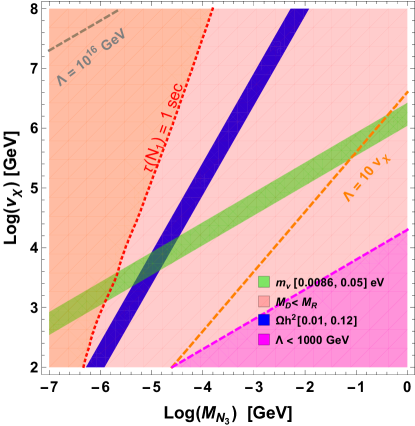
Figure 1: This plot represents constraints on $M_{N_{3}}$ and $v_{\chi}$ for Scenario-I. The blue band corresponds to the variation of the relic density from decay in between 0.01 and 0.12, where the latter satisfies the experimental constraint Aghanim:2018eyx . The green region corresponds to light neutrino mass in between 0.0086 eV to 0.05 eV. The red line corresponds to lifetime of $N_{1,2}$ as 1 second. The orange line correspond to $\Lambda>10.0\,v_{\chi}$. Here we assume the mass of the BSM Higgs as $M_{H_{2}}=250$ GeV.

In Fig. 1, we show the constraint on $v_{\chi}$ and on the DM mass $M_{N_{3}}$ that arise from requiring the relic density to lie in the range $0.01<\Omega h^{2}<0.12$ (blue region), namely we allow for $N_{3}$ to account for $10-100\%$ of the DM abundance. Here we include both $H_{1}\to N_{3}N_{3}$ and $H_{2}\to N_{3}N_{3}$ contributions to the relic density even though the $H_{2}$ contribution dominates as we fixed $M_{H_{2}}=250$ GeV. For this figure, we use the benchmark parameters given in Table. 1. Additionally, we also show the constraint from eV light neutrino mass in the same plot. For simplicity here and in other figures as well, we consider the light neutrino mass matrix $m_{\nu}$ (also $M_{D}$ and $M_{R}$) as a parameter, and impose neutrino mass constraint. Hence, $y$ denotes the Dirac Yukawa coupling parameter in Table. 1. The green shaded region is compatible with eV light neutrino masses , $0.0086\ \text{eV}<m_{\nu}<0.05\ \text{eV}$, while the seesaw approximation $M_{R}>M_{D}$ is satisfied in the entire plot. We further note that, following Eq. 24, for higher $v_{\chi}$ and lower $M_{N_{3}}$ the cutoff scale $\Lambda$ increases. The brown dashed line in the top left corner denotes $\Lambda=10^{16}$ GeV. We also show the line corresponding to $\Lambda=10v_{\chi}$ by orange dashed line. The magenta dashed line, assuming $\Lambda>1$ TeV rules out the region with large $M_{N_{3}}$ and low $v_{\chi}$ (magenta shaded region).

The constraint from the relic density depends on the Yukawa coupling $c_{33}$, which has been rewritten in terms of $M_{N_{3}}$. However, the constraint from eV light neutrino masses depend on other parameters, such as, $M_{N_{1,2}}$, and hence the couplings $c_{11},c_{22}$ as well as the Dirac Yukawa $y$. As can be seen from the figure, to satisfy the observed DM relic density, the required value $v_{\chi}$ increases with DM mass $M_{N_{3}}$. For GeV scale $M_{N_{3}}$, one needs $v_{\chi}>10^{8}$ GeV. This naturally leads to a very heavy BSM Higgs with mass $M_{H_{2}}\sim v_{\chi}>10^{8}$ GeV for the quartic scalar coupling $\lambda_{2}\sim 1$. This very heavy BSM Higgs does not have any detection prospect at collider. Contrary to that, the coupling $\lambda_{2}$ needs to be extremely tiny $\lambda_{2}<10^{-12}$ to accommodate $M_{H_{2}}\sim\mathcal{O}(100)$ GeV, which has better discovery prospect at the ongoing and future colliders. This unnatural fine-tuning relaxes, if the DM mass is $M_{N_{3}}\sim$ KeV. As can be seen from the figure, DM $N_{3}$ with few KeV mass is consistent with a $v_{\chi}\sim$ TeV and $\lambda_{2}\sim\mathcal{O}(0.1)$ and hence $M_{H_{2}}\sim\mathcal{O}(100)$ GeV. In conclusion, in Scenario-I we find that relic density constraint prefers a KeV scale DM and a TeV scale $v_{\chi}$ to naturally accommodate a BSM Higgs at the TeV scale or below.

$N_{1}$ and $N_{2}$ lifetime-

Before concluding the section we also discuss the lifetime of $N_{1,2}$. For the range of the relevant parameters that we consider in Fig. 1, the mass of the RHN states $N_{1,2}$ vary from $10^{-2}-10^{5}$ GeV, while the mixing $V$ ranges from $V\sim 10^{-4}-10^{-10}$. Here for simplicity, we consider $V$ as a parameter. For large mixing, $N_{1,2}$ state will thermalise and their decays would be constrained from the Big Bang Nucleosynthesis (BBN). While a detailed evaluation of the BBN bound is beyond the scope of this present paper, we however show the lifetime contour in Fig. 1 that corresponds to $\tau(N_{1,2})\sim 1$ sec. The two RHN states $N_{1,2}$ decay to various final states via their mixing $V$ with the active neutrinos. For masses much smaller than the pion mass, the decay mode would be $\nu\gamma$ and $\nu\nu\nu$. The decay width and lifetime for this mass range are

$$\tau^{-1}_{N_{1,2}} = \Gamma_{N_{1,2}}\simeq\frac{G^{2}_{F}M^{5}_{N_{1,2}}}{96\pi^{3}}V^{2}$$ (32)

$$= 5.16\times 10^{-24}\left(\frac{M_{N_{1,2}}}{keV}\right)^{5}\,\left(\frac{V^{2}}{10^{-7}}\right)s^{-1}.$$

For larger mass range $M_{N_{1,2}}>m_{\pi}+m_{e}$, additional decay modes $N\to l\pi^{\pm}$, $N\to lB^{\pm}/K^{\pm}$, and others will be open. For even higher mass range $M_{N_{1,2}}>M_{W},M_{Z},M_{H_{1,2}}$, the two body modes $N\to lW,\nu Z,\nu H_{1,2}$ will be open. The expressions for these decay widths are:

$$\Gamma_{N_{1,2}}(N\to l\pi)\simeq\frac{G^{2}_{F}M^{3}_{N_{1,2}}}{96\pi^{3}}V^{2}$$

(33)

$$\Gamma_{N_{1,2}}(N\to lW)\simeq\frac{g^{2}_{F}M^{3}_{N_{1,2}}}{64\pi M^{2}_{W}}V^{2}\left(1-\frac{M^{2}_{W}}{M^{2}_{N}}\right)^{2}\left(1+2\frac{M^{2}_{W}}{M^{2}_{N}}\right)$$ (34)

$$\Gamma_{N_{1,2}}(N\to\nu Z)\simeq\frac{g^{2}_{F}M^{3}_{N_{1,2}}}{128\pi M^{2}_{W}}V^{2}\left(1-\frac{M^{2}_{Z}}{M^{2}_{N}}\right)^{2}\left(1+2\frac{M^{2}_{Z}}{M^{2}_{N}}\right)$$ (35)

$$\Gamma_{N_{1,2}}(N\to\nu H_{1,2})\simeq\frac{g^{2}_{F}M^{3}_{N_{1,2}}}{128\pi M^{2}_{W}}V^{2}\left(1-\frac{M^{2}_{H_{1,2}}}{M^{2}_{N}}\right)^{2}$$ (36)

We evaluate the lifetime of $N_{1,2}$ assuming $M_{N_{1}}=M_{N_{2}}$ and show the contour of $\tau(N_{1,2})=1$ sec in Fig. 1 by the red line. Part of the region in the left side of the red line can be constrained from BBN as $N_{1,2}$ thermalise, and the decay of $N_{1,2}$ happens after $\tau(N_{1,2})=1$ sec. We estimate that for the region of Fig. 1 in agreement with both relic density and light neutrino mass, for which $M_{N_{3}}\sim 10-30$ KeV and $v_{\chi}\sim 4-10$ TeV, the cut-off scale $\Lambda\sim 10^{7}$ GeV, and the mixing angle $V\sim 10^{-6}$. Thus, $\tau(N_{1,2})<1$ sec, see Eq. 32, and the decay of $N_{1,2}$ in the early Universe occurs before BBN.

2.2 Scenario-II

We consider that in addition to the $N^{T}C^{-1}N\chi^{2}$ term, the Yukawa Lagrangian contains the term $N^{T}C^{-1}N\Phi^{\dagger}\Phi$. This is a more generic choice, as Scenario-I can be realised as only a special case of Scenario-II with $c^{\prime}=0$. The Lagrangian has the following terms:

$$\mathcal{L}_{eff}=\frac{c_{ij}}{\Lambda}N^{T}_{i}C^{-1}N_{j}\chi^{2}+\frac{c^{\prime}_{ij}}{\Lambda}N^{T}_{i}C^{-1}N_{j}\Phi^{\dagger}\Phi+ \frac{Y_{ij}}{\Lambda}\bar{L}_{i}\tilde{\Phi}N_{j}\chi+\textrm{h.c.}$$ (37)

In this scenario, the RHN neutrino masses get contributions from both the $NN\chi^{2}$ and $NN\Phi^{\dagger}\Phi$ terms. As before, we consider $c,c^{\prime}$ to be diagonal matrix. The mass matrix of the two RHN’s is

$$(M_{R})_{\alpha\beta}=\frac{c_{\alpha\beta}}{\Lambda}v^{2}_{\chi}+\frac{c^{\prime}_{\alpha\beta}}{\Lambda}v^{2}_{\Phi}~{}~{}~{}(\alpha,\beta=1,2)$$ (38)

The DM has a mass

$$M_{N_{3}}=\frac{c_{33}}{\Lambda}v^{2}_{\chi}+\frac{c^{\prime}_{33}}{\Lambda}v^{2}_{\Phi}$$ (39)

The Dirac mass matrix has the same expression as in the previous section, Eq. 16, and the physical mass matrix of $N_{1,2}$ follows $M_{N}\sim M_{R}$. With the seesaw condition $M_{R}>M_{D}$, the light neutrino mass matrix has a similar expression as Eq. 18. Below, we consider the couplings $c\sim c^{\prime}\simeq c_{0}$. Therefore, the light neutrino mass matrix receives a correction of $\mathcal{O}(\frac{v^{2}_{\Phi}}{v^{2}_{\chi}})$. The light neutrino and heavy RHN mass matrix have the following form,

$$m_{\nu} \sim -{Y}\frac{1}{c_{0}\Lambda}v^{2}_{\Phi}Y^{T}(1-\frac{v^{2}_{\Phi}}{v^{2}_{\chi}}),$$

$$M_{N} \sim \frac{c_{0}}{\Lambda}v^{2}_{\chi}(1+\frac{v^{2}_{\Phi}}{v^{2}_{\chi}})$$ (40)

Similar to the previous scenario, the RHN $N_{3}$ in this case is the FIMP DM. The particle is primarily produced from the two Higgs states $H_{1,2}$. The couplings of $N_{3}$ with $H_{1,2}$ states have the following form:

$$\tilde{\lambda}_{1}:-\frac{2v_{\chi}c_{33}}{\Lambda}\sin\theta+\frac{2v_{\Phi}c^{\prime}_{33}}{\Lambda}\cos\theta$$ (41)

$$\tilde{\lambda}_{2}:\frac{2v_{\chi}c_{33}}{\Lambda}\cos\theta+\frac{2v_{\Phi}c^{\prime}_{33}}{\Lambda}\sin\theta.$$ (42)

We first discuss two extreme scenarios,

• the $N_{3}N_{3}H_{1}$ coupling $\tilde{\lambda}_{1}$ is zero, i.e., the FIMP is produced only from $H_{2}$ decay.

• the $N_{3}N_{3}H_{2}$ coupling $\tilde{\lambda}_{2}$ is zero, i.e., the FIMP is produced from $H_{1}$ decay.

For the subsequent discussions, we consider the couplings $c$ and $c^{\prime}$ independently.

(a) In the first scenario, the DM is entirely produced from the Higgs state $H_{2}$. Imposing $\tilde{\lambda_{1}}=0$ in Eq. 41 leads to

$$\tan\theta=\frac{v_{\Phi}c^{\prime}_{33}}{v_{\chi}c_{33}}.$$ (43)

Using Eq. 43, $\tilde{\lambda}_{2}$ can be simplified as,

$$\tilde{\lambda}_{2}=\frac{2M_{N_{3}}}{(v_{\chi}\cos\theta+v_{\Phi}\sin\theta)}.$$ (44)

Using the above coupling in Eq. 28 we obtain the constraint on the vev $v_{\chi}$ from $\Omega h^{2}=0.12$,

$$v_{\chi}=\frac{1.22\times 10^{12}\ M_{N_{3}}^{3/2}}{M_{H_{2}}^{1/2}\cos\theta}-\frac{v_{\Phi}\sin\theta}{\cos\theta}.$$ (45)

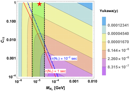
Figure 2: Left and Right panel: the figures correspond to scenario-IIa for two different Higgs masses $M_{H_{2}}=$250 GeV and 1.1 TeV, respectively. The color bar indicates the variation of Dirac Yukawa coupling $y$ w.r.t the variation of mass of FIMP DM $M_{N_{3}}$ and the Yukawa coupling $c_{11}$. The green band indicates variation of $v_{\chi}$ in between 1 TeV to 10 TeV (from left to right). See the texts for additional details.

Written in this way, the relic density constraint does not directly depend on the interaction coupling $c_{33}$ of the Yukawa Lagrangian, the dependency is only via $M_{N_{3}}$. Rather, the vev $v_{\chi}$ depends on the mass of the DM, Higgs mass, and the SM-BSM Higgs mixing angle $\theta$. The neutrino mass constraint, as we will derive, would be highly dependent on additional parameters. The constraint on the Dirac Yukawa is the same as Eq. 20, The mass of $N_{1}$ state (i.e., $M_{N_{1}}$) however gets additional contribution $c^{\prime}_{11}v^{2}_{\Phi}/\Lambda$ due to the $N_{3}N_{3}\Phi\Phi$ term.

$$M_{N_{1}}=({c_{11}v_{\chi}^{2}+c_{11}^{\prime}v_{\Phi}^{2}})/{\Lambda}$$ (46)

The cut-off scale $\Lambda$ can be written in terms of the mass of the DM,

$$\Lambda=\frac{c_{33}}{M_{N_{3}}}(v^{2}_{\chi}+\beta_{3}v^{2}_{\Phi}),$$ (47)

where $\beta_{3}=c^{\prime}_{33}/{c_{33}}$. We combine different constraints from Eq. 20, 43, 45, 46, 47 in Fig. 2, where we show the variation of the Dirac coupling $y$ in $M_{N_{3}}-c_{11}$ plane. For this, we choose a light neutrino mass $m_{\nu}=0.05$ eV, a Higgs mixing $\sin\theta=0.1$, $M_{H_{2}}=250$ GeV (left panel), and $1.1$ TeV (right panel). Moreover we assume $c_{11}^{\prime}=1$ and $c_{33}^{\prime}=2.5\times 10^{-6}$. We have checked that for this choice of parameters the coupling $c_{33}$ which dictates $M_{N_{3}}$, is perturbative in the entire region. We also display the region where $v_{\chi}$ is in the range 1-10 TeV. In Fig. 2, this is shown as the vertical green band as $v_{\chi}$ depends on $M_{N_{3}}$ but not on $c_{11}$. The cut-off scale also increases with $M_{N_{3}}$, we checked (using Eq. 43, 45) that at the boundary of the green band $\Lambda=(1,\ 2)\times 10^{6}$ GeV for left panel, and $\Lambda=(7,\ 14)\times 10^{5}$ GeV for the right panel.

It is evident from Fig. 2, that the choice of a large DM mass, $M_{N_{3}}$, together with a larger $c_{11}$ demands a larger coupling $y$ after imposing the light neutrino mass and relic density constraints. In the entire region the seesaw condition $M_{R}>M_{D}$ is satisfied. The red and blue lines represent the lifetime of $N_{1,2}$ as 1 sec and $10^{-2}$ sec, respectively for the left and for the right panel. The region enclosed by the red dashed line in the right plot corresponds to $\tau(N_{1})>1$ sec.

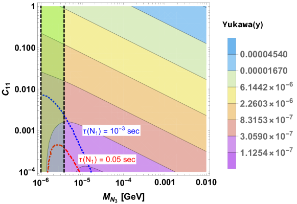
Figure 3: The figure corresponds to Scenario-IIb, and represents the variation of the Yukawa coupling $y$ w.r.t the variation of the DM mass $M_{N_{3}}$ and the Yukawa coupling $c_{11}$. Contours of $\tau(N_{1,2})=0.001$ (blue) and 0.05 (red) are displayed. The vertical black lines correspond to $v_{\chi}=3$ TeV (left) and 10 TeV (right).

(b) The other scenario is where DM is produced from the SM Higgs. This can be realised for a suppressed $N_{3}N_{3}H_{2}$ coupling, we will consider the limit where this coupling is zero leading to the following constraint,

$$\tan\theta=-\frac{c_{33}v_{\chi}}{c^{\prime}_{33}v_{\Phi}}.$$ (48)

Using Eq. 48, $\tilde{\lambda}_{1}$ can be simplified to the form,

$$\tilde{\lambda}_{1}=\frac{-2M_{N_{3}}}{(v_{\chi}\sin\theta-v_{\Phi}\cos\theta)}$$ (49)

Using above coupling in Eq. 28 we get,

$$v_{\chi}={\color[rgb]{0,0,1}\pm}\frac{1.22\times 10^{12}\ M_{N_{3}}^{3/2}}{M_{H_{1}}^{1/2}\sin\theta}+\frac{v_{\Phi}\cos\theta}{\sin\theta}$$ (50)

In the above, the $+\text{ and}-\text{ sign correspond to }(v_{\chi}\sin\theta-v_{\Phi}\cos\theta)>0\text{ and}<0$, respectively.

The constraint on the Dirac Yukawa in this case remains as in Eq. 20, where the cut-off scale $\Lambda$ and the mass of the DM are related by Eq. 47. In Fig. 3 we plot the Dirac Yukawa as a function of $c_{11}$ and $M_{N_{3}}$. As before we consider the parameter $\sin\theta=0.1$. Additionally, we consider $c^{\prime}_{11}=1,c^{\prime}_{33}=-10^{-6}$. The Yukawa coupling $c_{33}$ varies with $M_{N_{3}}$, and is perturbative in the entire range of $M_{N_{3}}$. The seesaw condition $M_{D}<M_{R}$ is satisfied in the entire parameter space. The green band bounded by black dashed lines represent the variation of $v_{\chi}$ ($\Lambda$) between 3 TeV ($2\times 10^{4}$ GeV) and 10 TeV ($5\times 10^{4}$ GeV), from left to right. The lifetime of $N_{1,2}$ is less than 1 sec in the entire range. For illustration, the blue and red dashed lines indicate lifetime of $N_{1,2}$ as 0.001 sec, and $0.05$ sec, respectively.

Figure 4: Similar as the Fig. 1, but for Scenario-II. See text for more details.

We also consider the generic scenario where both the $H_{1}\to N_{3}N_{3}$ and $H_{2}\to N_{3}N_{3}$ contribute to the relic density. In Fig. 4, we show different constraints in the $v_{\chi}-M_{N_{3}}$ plane. The blue band represents the total contribution from $H_{1}\to N_{3}N_{3}$ and $H_{2}\to N_{3}N_{3}$ which varies in the mentioned range. The green band represents the constraint from light neutrino mass. While the relic density constraint does not depend on the Yukawa $y$, the latter depends on few additional parameters. See Table. 1 for the details of the input parameters. Similar to Scenario-I, we represent $\tau(N_{1,2})=1$ sec by red line, cut off scale $\Lambda=10v_{\chi}$ by orange line. The point represented by a red star mark in this plot, corresponds to the star point shown in the left panel of Fig. 2, representing the same benchmark point. Similar to the previous scenario Scenario-I, a higher vev $v_{\chi}$ is required to satisfy relic abundance for a heavier DM mass. This happens, as for both these two scenarios, the DM mass is governed by the vev $v_{\chi}$, which also governs the $H_{1,2}\to N_{3}N_{3}$ coupling, and hence the DM production. Therefore, a TeV scale $v_{\chi}$ together with a TeV scale BSM Higgs with mass $M_{H_{2}}$ demand that the DM mass in this case can be at most $M_{N_{3}}\sim\textrm{few}$ KeV. We will see in the next section, how addition of a bare mass term in the Lagrangian relaxes this strong correlation.

2.3 Scenario-III

The DM phenomenology changes if a bare mass term for the FIMP DM $N_{3}$ state is being added to the Lagrangian. In this case, the tight correlation between the DM mass and vev of the gauge singlet scalar relaxes. Adding a bare mass term $M_{B}$ for $N_{1,2,3}$, the Lagrangian has the following form,

$$\mathcal{L}_{eff} = \frac{c_{ij}}{\Lambda}N^{T}_{i}C^{-1}N_{j}\chi^{2}+\frac{c^{\prime}_{ij}}{\Lambda}N^{T}_{i}C^{-1}N_{j}\Phi^{\dagger}\Phi$$ (51)

$$+\frac{Y_{ij}}{\Lambda}\bar{L}_{i}N_{j}H\chi+M_{B}N^{T}_{i}C^{-1}N_{i}+h.c$$

In the above, $M_{B}$ is a diagonal mass matrix $M_{B}=(M_{B_{1}},M_{B_{2}},M_{B_{3}})$, that represents the bare mass term for RHNs. The RHN mass matrix of $N_{1,2}$ can be written as follows,

$$(M_{R})_{\alpha\beta}=\frac{c_{\alpha\beta}v_{\chi}^{2}}{\Lambda}+\frac{c^{\prime}_{\alpha\beta}v_{\phi}^{2}}{\Lambda}+(M_{B})_{\alpha\beta}~{}~{}(\alpha,\beta=1,2).$$ (52)

Hence, the DM mass is

$$M_{N_{3}}=\frac{c_{33}v_{\chi}^{2}}{\Lambda}+\frac{c^{\prime}_{33}v_{\phi}^{2}}{\Lambda}+M_{B_{3}}.$$ (53)

Note that, for $c_{33}$ and $c^{\prime}_{33}$ of $\mathcal{O}(1)$, the mass of $N_{3}$ can primarily be governed by $M_{B_{3}}$, and the other two terms can provide sub-dominant contributions. The Dirac mass matrix have the same form as in previous scenarios, Eq. 16, and as before, $M_{N}\sim M_{R}$. The light neutrino mass matrix has the following expression,

$$m_{\nu} \sim -\frac{1}{\Lambda}\frac{{Y}v^{2}_{\Phi}v_{\chi}^{2}Y^{T}}{c_{11}v_{\chi}^{2}+c^{\prime}_{11}v_{\phi}^{2}+\Lambda M_{B_{1}}},$$ (54)

where we again consider $M_{N_{1}}=M_{N_{2}}$.

Scenario-III
$M_{H_{2}}$	$\sin\theta$	$y$	$c_{33}\ (=c^{\prime}_{33})$	$M_{N_{3}}-M_{B_{3}}$	$M_{N_{1}}$
$250$ GeV	$0.1$	$1$	$10^{-4}$	$10^{-8}$ GeV	$4M_{N_{3}}$

Table 2: The parameters relevant for Scenario-III, Fig. 5.

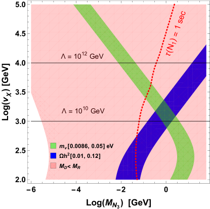
Figure 5: Scenario-III: Constraints from the DM relic density (blue band) and eV scale light neutrino mass (green band) in the $M_{N_{3}}-v_{\chi}$ plane. The values of other free parameters are listed in Table 2 . Here we include the decay of $H_{1,2}$ for DM production.

DM production-

In this scenario, the DM can be produced from $H_{1,2}\to N_{3}N_{3}$ decays. The interaction vertex of $N_{3}$ with $H_{1,2}$ states have the same form as given in Eq. 41, and Eq. 42. As in previous scenarios we consider two extreme cases where a) $\tilde{\lambda}_{1}$=0 and the DM is produced from $H_{2}$ decay. b) $\tilde{\lambda}_{2}=0$ and the DM is produced from $H_{1}$ decay.

1. The condition $\tilde{\lambda}_{1}=0$ together with Eq. 43 leads to the $N_{3}N_{3}H_{2}$ coupling

   $$\tilde{\lambda}_{2}=\frac{2(M_{N_{3}}-M_{B_{3}})}{(v_{\chi}\cos\theta+v_{\Phi}\sin\theta)}.$$ (55)

   and to the constraint on the vev $v_{\chi}$

   $$v_{\chi}=\frac{1.22\times 10^{12}\ (M_{N_{3}}-M_{B_{3}})^{3/2}}{M_{H_{2}}^{1/2}\cos\theta}-\frac{v_{\Phi}\sin\theta}{\cos\theta}.$$ (56)

2. The condition $\tilde{\lambda}_{2}=0$ together with Eq. 48 leads to the $N_{3}N_{3}H_{2}$ coupling

   $$\tilde{\lambda}_{1}=-\frac{2(M_{N_{3}}-M_{B_{3}})}{(v_{\chi}\sin\theta-v_{\Phi}\cos\theta)}.$$ (57)

   and to the constraint on the vev $v_{\chi}$

   $$v_{\chi}=\pm\frac{1.22\times 10^{12}\ (M_{N_{3}}-M_{B_{3}})M_{N_{3}}^{1/2}}{M_{H_{1}}^{1/2}\sin\theta}+\frac{v_{\Phi}\cos\theta}{\sin\theta}.$$ (58)

For both the scenarios $a$ and $b$, it is evident that the factor $M_{N_{3}}-M_{B_{3}}$ in the numerator of Eq. 56 and Eq. 58 will have impact on the tight correlation between $v_{\chi}$ and $M_{N_{3}}$, found in Scenario-I-II.

In general both $H_{1}\to N_{3}N_{3}$ and $H_{2}\to N_{3}N_{3}$ can contribute to the relic density. With the choice of input parameters given in Table 2, the constraints on $M_{N_{3}}$ and $v_{\chi}$ are shown in Fig. 5. The pink colour shaded area indicates that seesaw approximation $M_{R}>M_{D}$ is satisfied. In the blue band, DM relic density varies in the range $0.01<\Omega h^{2}<0.12$ from left to right. The green band represents the constraint from light neutrino mass while the red dashed line corresponds to the contour $\tau(N_{1,2})=1$ sec. The horizontal lines represent the cut-off scale $\Lambda=10^{10}$ and $10^{12}$ GeV. From Fig. 5 it can be seen that the region compatible with both the relic density and the neutrino mass constraints corresponds to $v_{\chi}\sim\cal O$(TeV) and $M_{N_{3}}\sim\cal O$(GeV). In this scenario it is therefore natural to have a BSM Higgs at the TeV scale for a coupling $\lambda_{2}\sim{\cal O}(1)$. In Section 4 we will consider this scenario and explore the collider signature of a TeV scale BSM Higgs.

3 DM production : decay vs annihilation

In the previous sections we considered only decay contributions of the SM and BSM Higgs in the relic density. This is justified for a not too large reheating temperature $T_{R}$ Hall:2009bx . In this section we deviate from this assumption and allow for a high $T_{R}$. Thus we obtain larger contributions from annihilation channels as well. To determine the co-moving number density of $N_{3}$, we need to solve the following Boltzmann equation,

$$\dfrac{dY_{N_{3}}}{dz}=\dfrac{2M_{pl}}{1.66M_{H_{2}}^{2}}\dfrac{z\sqrt{g_{\star}(z)}}{g_{s}(z)}\,\,\Bigg{[}\sum_{i=1,\,2}\langle\Gamma_{H_{i}\rightarrow N_{3}N_{3}}\rangle(Y_{H_{i}}^{eq}-Y_{N_{3}})\Bigg{]}$$

$$~{}~{}~{}~{}~{}~{}~{}~{}~{}+\dfrac{4\pi^{2}}{45}\dfrac{M_{pl}M_{H_{2}}}{1.66}\dfrac{\sqrt{g_{\star}(z)}}{z^{2}}\,\,\Bigg{[}\sum_{x=W,Z,h_{1},h_{2},f}\langle\sigma{\rm v}_{x\bar{x}\rightarrow N_{3}N_{3}}\rangle(Y_{x}^{eq\,\,2}-Y_{N_{3}}^{2})\Bigg{]}$$ (59)

where $z=M_{H_{2}}/T$ and $g_{*}(z)$ depends on $g_{s}(z)$, $g_{\rho}(z)$ in the following way Gondolo:1990dk , $\sqrt{g_{*}(z)}=\frac{g_{s}(z)}{\sqrt{g_{\rho}(z)}}\left(1-\frac{1}{3}\frac{d\,{\rm ln}\,g_{s}(z)}{d\,{\rm ln}\,z}\right)\,.$ $Y_{A}$ is the co-moving number density of $A$, $M_{pl}$ is the Planck mass and the quantity inside $<...>$ corresponds to the thermal average of decay rate and annihilation cross-sections. From the co-moving number density obtained by solving the Eq. 59, one can determine the relic density of DM by following the expression,

$$\Omega_{N_{3}}h^{2}=2.755\times 10^{8}\,\left(\dfrac{M_{N_{3}}}{\rm GeV}\right)\,Y_{N_{3}}(T_{0})\,,$$ (60)

We perform our numerical simulation using micrOMEGAs5.0 Belanger:2018ccd after implementing the model file in Feynrules Alloul:2013bka .

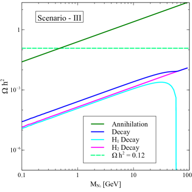
Figure 6: Left (right) panel : $\Omega h^{2}$ vs the mass of DM for Scenario-III (Scenario-II) with $\sin\theta=0.1$, $\Lambda=10^{11}$ GeV, $M_{H_{2}}=1100$ GeV, $M_{N_{1,2}}=5M_{N_{3}}$, $M_{N_{3}}-M_{B_{3}}=10^{-8}$ GeV, $v_{\chi}=3$ TeV (left panel), $M_{B_{3}}=0$, $v_{\chi}=15$ TeV (right panel). The green-dashed horizontal line represents $\Omega h^{2}=0.12$ Aghanim:2018eyx .

In the left and right panel of Fig. 6, we show the variation of the DM relic density with its mass for Scenario-III and Scenario-II, respectively. We keep the other parameters fixed as shown in the caption. For these figures, we choose a high value of the reheating temperature, $T_{R}=10^{9}$ GeV. From both the figures, one can see that the DM relic density increases with its mass $M_{N_{3}}$ as also evident from Eq. 60. In the left panel, there is a sharp fall in the $H_{1}$ decay contribution at $M_{N_{3}}=\frac{M_{H_{1}}}{2}$ when the $H_{1}$ decay to DM is not kinematically allowed. Note that for large $T_{R}$ the annihilation contribution is larger than the decay contribution by several orders of magnitude. This occurs as relic density for annihilation (from $WW/ZZ\to N_{3}N_{3},\ H_{i}H_{j}\to N_{3}N_{3}$) is proportional to the value of the reheating temperature as shown in the Appendix, see Eq. 76.

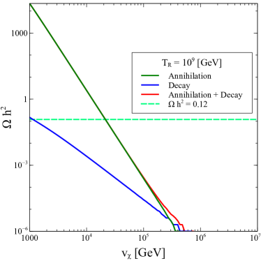
Figure 7: Left panel: Relic density vs reheating temperature for Scenario-III. Right panel: variation of relic density vs vev of the singlet scalar for the same scenario. Other parameters kept fixed at $\sin\theta=0.1$, $\Lambda=10^{11}$ GeV, $M_{H_{2}}=1100$ GeV, $M_{N_{1,2}}=5M_{N_{3}}$, $M_{N_{3}}-M_{B_{3}}=10^{-8}$ GeV and $v_{\chi}=3000$ GeV. The green dashed horizontal line represents the experimental constraint on DM relic density Aghanim:2018eyx .

We also show the variation of relic density with the reheating temperature $T_{R}$ (shown in the left panel), and the vev $v_{\chi}$ (shown in the right panel) in Fig. 7. Moreover, the individual contributions from decay and annihilation processes to the total relic density have also been shown in both the panels. In the left panel, we can see that the decay contribution does not depend on the reheating temperature, $T_{R}$, but annihilation contribution strongly depends on the reheating temperature when $T_{R}\mathrel{\mathop{\kern 0.0pt\hbox to0.0pt{\raise 0.86108pt\hbox{$>$}\hss}}\lower 3.87495pt\hbox{\kern-1.90002pt$\sim$}}10^{6}$ GeV. As we have shown in Eq. 76 of the Appendix, and also have been discussed in Hall:2009bx , the annihilation contribution depends on the reheating temperature and linearly grows with it. This is visible in Fig. 7, where for large $T_{R}$ annihilation contributions increase. This occurs because of the presence of $d=5$ $H_{i}H_{j}N_{3}N_{3}$ ($i,j=1,2$) operators. We also show in the Appendix that $WW/ZZ\to N_{3}N_{3}$ exhibits similar feature. Furthermore, as evident from Eq. 77, the contribution from the annihilation process $f\bar{f}\rightarrow N_{3}N_{3}$ is dominated by the low scale physics. For a very high $T_{R}$ this contribution becomes almost independent of the variation of $T_{R}$. In the right panel of Fig. 7, the variation of relic density with the vev $v_{\chi}$ has been shown. One can see that both decay and annihilation contributions fall linearly with the increase of the $v_{\chi}$. This can be explained easily, as the coupling of DM with the Higgs is inversely proportional to the square of the vev i.e. $\tilde{\lambda}_{1,2}\propto\frac{1}{v^{2}_{\chi}}$. In addition, the $WW\to N_{3}N_{3},ZZ\to N_{3}N_{3}$ contributions also depend on the coupling $\tilde{\lambda}_{1,2}$. Moreover the contact interaction $H_{i}H_{i}\to N_{3}N_{3}$ depends on $c_{33}/\Lambda$, which also varies as $1/v_{\chi}$. Therefore, as the vev increases, the relevant coupling becomes smaller, resulting in a reduced production of DM.

3.1 The parameter space of Scenario-III

In the previous section, we have evaluated the decay and annihilation contributions to the relic density for specific benchmark points. In this section we vary all the free parameters of Scenario-III in a wide range and present the results in the form of scatter plots. The model parameters are varied in the following range,

$$200\,\,{\rm GeV}\,\,< M_{H_{2}} <3000\,\,{\rm GeV}$$ (61)

$$10\,\,{\rm GeV}\,\,< M_{N_{3}} <100\,\,{\rm GeV}$$

$$10^{-3}< \theta <10^{-1}$$

$$1000\,\,{\rm GeV}\,\,< v_{\chi} <10000\,\,{\rm GeV}$$

$$200\,\,{\rm GeV}\,\,< T_{R} <10^{9}\,\,{\rm GeV}$$

$$10^{9}\,\,{\rm GeV}\,\,< \Lambda <10^{14}\,\,{\rm GeV}\,.$$

To accommodate $H_{2}$ at the TeV scale together with $v_{\chi}\sim$TeV, the bare mass term of $N_{3}$ has to dominate its physical mass $M_{N_{3}}$, thus we impose $M_{N_{3}}-M_{B_{3}}\sim\mathcal{O}(10^{-8})$ GeV. In our scan we require that $N_{3}$ contribute to at least $10\%$ of the total DM, thus we impose that its relic density falls within the range

$$0.01<\Omega h^{2}<0.1211.$$ (62)

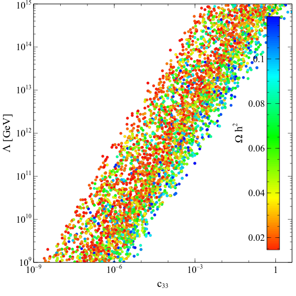
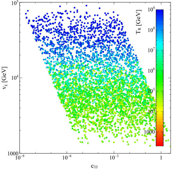
Figure 8: Left panel: variation of relic density of $N_{3}$ in the $c_{33}-\Lambda$ plane. Right panel: variation of $T_{R}$ in the $c_{33}-v_{\chi}$ plane. We consider the same constraint as in the left panel.

In Fig. 8, 9 we display the allowed parameter space after taking into account the constraint from Eq. 62. The entire range of $M_{N_{3}}$ mentioned above can satisfy Eq. 62 with the variation of other model parameters. We did not find any strong correlation between $M_{N_{3}}$ and other model parameters, and hence we do not present any scatter plot for $M_{N_{3}}$.

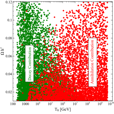
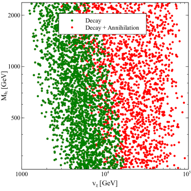
Figure 9: Left panel: Variation of relic density of $N_{3}$ vs $T_{R}$. Right panel: scatter plot in the $v_{\chi}-M_{H_{2}}$ plane.

In the left panel of Fig. 8, we show the variation of relic density (in color bar) in the $c_{33}-\Lambda$ plane after satisfying Eq. 62. For Scenario-III, we can express the coupling $c_{33}$ in terms of the cut off scale $\Lambda$ and the vevs $v_{\phi},v_{\chi}$ in the following way,

$$c_{33}=\frac{\Lambda(M_{N_{3}}-M_{B_{3}})}{v^{2}_{\chi}+\beta_{3}v^{2}_{\phi}}\,.$$ (63)

As evident from the above expression, there is a linear relation between $c_{33}$ and $\Lambda$. Therefore, as we increase $\Lambda$, $c_{33}$ also increases. This is clearly visible from the figure shown in the left panel. The blue scattered points satisfy the experimentally measured DM relic density constraint Aghanim:2018eyx . In the right panel of Fig. 8, we show the points that satisfy Eq. 62 in the $v_{\chi}-c_{33}$ plane. As expected from Eq. 63, since $v_{\chi}\gg\beta_{3}v_{\phi}$, $c_{33}$ is inversely proportional to $v_{\chi}^{2}$. Furthermore, right panel of Fig. 8 shows that $T_{R}$ increases linearly with $v_{\chi}$. This can be understood as follows. We have seen in Fig. 7 that the relic density (when dominated by the annihilation contribution) increases with the reheating temperature at large $T_{R}$, and decreases as $1/v_{\chi}$. Therefore, for a given value of the DM relic density, higher values of $T_{R}$ will be associated with larger values of $v_{\chi}$. The yellow points are not clearly visible, as they have been covered by the green points.

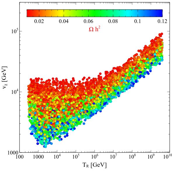
Figure 10: Variation of relic density w.r.t variation of $v_{\chi}$ and $T_{R}$. The points satisfy the mentioned DM relic density range.

In the left panel of Fig. 9, we show the variation of the decay and annihilation contributions to the relic density with $T_{R}$. For the discussion on the dependency of the relic density on $T_{R}$, see Section. Appendix. In the right panel of the same plot, we show the relation between $v_{\chi}$ and $M_{H_{2}}$. As evident from the left plot, for reheating temperature $T_{R}\sim 10^{5}$ GeV, the decay and annihilation contributions are equal, while for $T_{R}>10^{6}-10^{7}$ GeV, the annihilation contributions dominate. Lower than $T_{R}\sim 10^{5}$ GeV, decay contribution to the relic density dominates. This occurs as the annihilation contribution is directly proportional to the reheating temperature as has been explained before. In generating the scatter plots both for Fig. 8 and Fig. 9, we assume that the reheating temperature is greater than the masses of all the particles.

In the right panel of Fig. 9, we show the points in the $v_{\chi}-M_{H_{2}}$ plane which satisfy Eq. 62. We represent the decay contribution by green points and the total contribution by red points. For the decay contribution, there exists an inverse correlation between $v_{\chi}$ and $M_{H_{2}}$. The $H_{2}N_{3}N_{3}$ coupling for this case takes the following form,

$$\tilde{\lambda}_{2}=\frac{2(M_{N_{3}}-M_{B_{3}})\times(v_{\chi}\cos\theta+\beta_{3}v_{\phi}\sin\theta)}{v^{2}_{\chi}+\beta_{3}v^{2}_{\phi}}\,.$$ (64)

The above equation together with Eq. 30 imply that the DM relic density decreases with the increase of both $v_{\chi}$ and $M_{H_{2}}$. Therefore, for a given value of the DM relic density, higher values of $v_{\chi}$ will be associated with smaller values of $M_{H_{2}}$. For annihilation processes the correlation between $v_{\chi}$ and $M_{H_{2}}$ is somewhat mild, as the additional parameter $T_{R}$ plays a significant role in annihilation processes, and we have varied $T_{R}$ in a wide range mentioned in Eq. 61.

$\sigma$ (pb)	$M_{H_{2}}=250$ GeV	$M_{H_{2}}=500$ GeV	$M_{H_{2}}=1100$ GeV
$\sigma(pp\to H_{2}\to ZZ)$	$<0.12$	$<0.02$	$<0.005$
$\sigma(pp\to H_{2}\to VV)$	$<1.6$ ($M_{H_{2}}=300$ GeV)	$<0.2$	$<0.008$
$\sigma(pp\to H_{2}\to H_{1}H_{1})$	$<0.8\ (3)$	$<0.15\ (0.25)$	$<0.03\ (0.04)$
$\sigma(pp\to H_{2}jj\to H_{1}H_{1}jj)$	$<1$	$<0.05$	$<0.004$ ($M_{H_{2}}=1$ TeV)

Table 3: LHC constraints on BSM Higgs production in GF and VBF channel. We follow Aad:2020fpj for $ZZ$ channel (ATLAS search-139 $\rm{fb}^{-1}$), Aad:2020ddw for $VV\ (WW+ZZ)$ channel (ATLAS search-139 $\rm{fb}^{-1}$), Aad:2019uzh for $H_{1}H_{1}$ (ATLAS search-36.1 $\rm{fb}^{-1}$), and Aad:2020kub for $H_{1}H_{1}+jj$ channel (ATLAS search-126 $\rm{fb}^{-1}$). For $H_{1}H_{1}$ channel, the limits from CMS search-35.9 $\rm{fb}^{-1}$  Sirunyan:2018zkk are mentioned in bracket, that we obtained after deviding $\sigma(pp\to H_{2}\to H_{1}H_{1}\to 4b)$ by $Br^{2}(H_{1}\to b\bar{b})$.

Finally in Fig. 10, we show the variation of the relic density w.r.t to the variation of vev $v_{\chi}$ and the reheating temperature $T_{R}$. As we have discussed, the coupling strength to produce DM varies inversely with the vev, therefore for a smaller vev, the coupling $c_{33}$ increases. This results in a higher value of the $\Omega h^{2}$ which is represented by the blue points. We can also see for $T_{R}>10^{6}$ GeV there exist a sharp correlation between $T_{R}$ and $v_{\chi}$, which is consistent with the right panel of Fig. 8.

4 Collider Signature of $H_{2}$

Other than the SM Higgs, the model also contains a neutral BSM Higgs, which can be probed at collider experiments. A number of LHC measurements constrain the presence of such a heavy Higgs, and its mixing with the SM 125 GeV Higgs Sirunyan:2018koj . For the collider analysis we consider BSM Higgs in the TeV mass range. We pursue the study for Scenario-III. The model signature we study will remain the same for Scenario-I, and II as well, as the signature does not depend on DM mass. The LHC searches that constrain the BSM Higgs and its mixing are - a) The SM Higgs signal strength measurement, and b) heavy Higgs searches.

a) Higgs signal strength measurement constrains the mixing of the SM and BSM Higgs. To evaluate this, we adopt Sirunyan:2018koj . The signal strength of SM Higgs is given as,

$$\mu_{h\rightarrow xx}=\frac{\sigma_{H_{1}}}{\sigma_{H_{1}}^{SM}}\frac{Br(H_{1}\rightarrow xx)}{Br^{SM}(H_{1}\rightarrow xx)}$$ (65)

In the above, $H_{1}\rightarrow xx$ represents any channel where SM Higgs can decay. In our model one of the additional final states in which SM Higgs can decay is to DM pair ($H_{1}\to N_{3}N_{3}$). However, the branching ratio of this channel is very small $Br(H_{1}\rightarrow N_{3}N_{3})<10^{-8}$. The other modes such as $H_{1}\rightarrow\nu N_{1,2}/N_{1}N_{1}/N_{2}N_{2}$ also have small branching ratios. Therefore, for all practical purposes, these channels can be neglected. The branching ratio of $H_{1}$ decaying to any SM final state is hence almost identical to the branching ratio in the SM, i.e., $Br(H_{1}\rightarrow xx)\sim Br^{SM}(H_{1}\rightarrow xx)$. The production cross-section of $pp\to H_{1}$ becomes $\sigma_{H_{1}}=\cos^{2}\theta\sigma_{H_{1}}^{SM}$. Therefore, we find that the above Higgs signal strength expression takes a very simplified form,

$$\mu_{H_{1}\rightarrow xx}\sim\cos^{2}\theta.$$ (66)

The $\sqrt{s}=13$ TeV LHC measurements of the Higgs signal strength in combined channel dictates $\mu=1.17\pm 0.1$ Sirunyan:2018koj . We find, allowing a $3\sigma$ deviation around the best fit value of $\mu=1.17$, that the Higgs mixing angle $\sin\theta<0.36$. In our subsequent analysis, we consider both a larger value of $\sin\theta=0.34$ and a small value, $\sin\theta=0.1$.

b) A number of LHC searches constrain the production of heavy scalar resonance and its decay into various SM final states. As discussed in the previous sections, one of the main production channels of the FIMP DM is the decay of $H_{2}$ to two $N_{3}$ states, which is dominant for a low reheating temperature. However, due to the negligible branching ratio $Br(H_{2}/H_{1}\to N_{3}N_{3})<10^{-8}$, this channel is not constrained by the LHC searches for the invisible decays of Higgs. The main decay channels of the BSM Higgs include $H_{2}\to WW,ZZ,b\bar{b},\tau^{+}\tau^{-},H_{1}H_{1}$ channels. A number of CMS and ATLAS searches constrain the production cross-section of the BSM Higgs in gluon fusion (GF), or vector boson fusion (VBF) channels folded with the branching ratio of the $H_{2}$ in the above mentioned modes. In Table. 3, we outline the most sensitive searches for a neutral Higgs at the LHC, where we quote the limits on $\sigma\times Br$ for few illustrative mass points. We consider the searches $pp\to H_{2}\to ZZ$ Aad:2020fpj , $pp\to H_{2}\to W^{+}W^{-}+ZZ$ Aad:2020ddw , $pp\to H_{2}\to H_{1}H_{1}\to 4b$ Aad:2019uzh ; Sirunyan:2018zkk , $pp\to H_{2}+jj\to H_{1}H_{1}+jj$ Aad:2020kub . We find that among them $pp\to H_{2}\to ZZ$ Aad:2020fpj is most constraining, in particular this channel does not allow lighter masses, $M_{H_{2}}\sim 200$ GeV, for larger value of $\sin\theta=0.34$. Note that this mixing angle is allowed by Higgs signal strength measurements. Such values are marginally allowed by the search $pp\to H_{2}\to VV$. On the other hand, the large mixing angle, $\sin\theta\sim 0.34$ is allowed by all the above mentioned searches when $M_{H_{2}}\sim 1$ TeV. The mixing angle $\sin\theta=0.1$ which we consider for the DM analysis in the previous section is allowed for the entire range $200\,\textrm{GeV}<M_{H_{2}}<\textrm{few}$ TeV. We have cross-checked our results with the results obtained from HiggsBound Bechtle:2020pkv .

Other than the $WW,ZZ$ channels, one of the spectacular signature of a heavy BSM scalar is the di-Higgs signal. The di-Higgs channel is in-particular important to probe Higgs tri-linear coupling. Any deviation from the SM prediction will indicate new physics. Di-Higgs production in SM, which is non-resonant, has extensively been studied for LHC. There are different studies that analysed $b\bar{b}\gamma\gamma$Baur:2002qd ; Baur:2003gp ; Azatov:2015oxa ; Kling:2016lay , $b\bar{b}W^{+}W^{-}$Dolan:2012rv ; Papaefstathiou:2012qe , $b\bar{b}\tau^{+}\tau^{-}$Dolan:2012rv ; Barr:2013tda ; Banerjee:2018yxy , $b\bar{b}b\bar{b}$deLima:2014dta ; Wardrope:2014kya ; Behr:2015oqq ; Banerjee:2018yxy , and $b\bar{b}+E_{T}$Banerjee:2016nzb final states. With a heavy BSM Higgs which couples to two SM Higgs, the di-Higgs production cross-section becomes large. The studies Dolan:2012ac ; No:2013wsa ; Martin-Lozano:2015dja ; Huang:2017jws ; Ren:2017jbg ; Basler:2019nas ; Li:2019tfd ; Adhikary:2018ise ; Lu:2015qqa ; Alves:2019igs focus on resonant production of a BSM Higgs and its decay to di-Higgs. Both resonant and non-resonant di-Higgs production processes have been extensively explored by CMS and ATLAS Aaboud:2016xco ; Khachatryan:2016cfa ; Khachatryan:2016sey ; Aad:2015xja ; Aaboud:2018knk ; Aaboud:2018zhh ; Aaboud:2018sfw ; Aaboud:2018ksn ; Aaboud:2018ftw ; Aaboud:2018ewm ; Aad:2019uzh . Most of the above mentioned studies focused on the resolved final states with isolated final state leptons, jets, and photons. However, for a very heavy mass of the BSM Higgs, the produced SM Higgs will be boosted, leading to collimated decay products. Note that, the di-Higgs production from a heavy Higgs with few TeV mass is less favourable at $\sqrt{s}=13$ TeV LHC due to smaller production cross section. For non-resonant di-Higgs production at the proposed $\sqrt{s}=100$ TeV LHC, see Cao:2016zob ; Chang:2018uwu ; Mangano:2020sao ; Park:2020yps ; Borowka:2018pxx .

We instead focus on resonant di-Higgs production from the decay of a heavy BSM Higgs at $100$ TeV collider, decaying into two SM Higgs. The branching ratio of this channel $Br(H_{2}\rightarrow H_{1}H_{1})\sim 25\%$ for $H_{2}$ mass around $1\,\rm TeV$ Banerjee:2015hoa . We analyse the di-Higgs channel with subsequent decay of $H_{1}$ to $b\bar{b}$. We assume $M_{H_{2}}>1$ TeV, for which the two Higgs bosons produced from $H_{2}$ are moderately boosted, leading to a peak in $\Delta R$ separation between the two $b$ quarks as $\Delta R(b,\bar{b}\lesssim 0.4)$. Instead of a resolved analysis with four or more number of isolated $b$ jets in the final state, we perform an analysis where we adopt a large radius jet as the jet description, which is effective in suppressing a number of SM backgrounds. Therefore, our model signature is

$$pp\to H_{2}\to H_{1}H_{1}\to 2j_{\textrm{fat}}.$$ (67)

where, each of the fatjet $j_{\textrm{fat}}$ contains two $b$ quarks appearing from Higgs decay.

To evaluate the signature, we implement the Lagrangian of this model in FeynRules(v2.3)   Alloul:2013bka to create the UFO Degrande:2011ua model files. The Event generator MadGraph5_aMC@NLO(v2.6) Alwall:2014hca is used to generate both the signal and the background events at leading order. Generated events are passed through Pythia8 Sjostrand:2014zea to perform showering and hadronization. Detector effects are simulated using Delphes (v3.4.1) deFavereau:2013fsa . We use FastJet Cacciari:2011ma for the clustering of fatjets and consider Cambridge-Achen Dokshitzer:1997in ; Wobisch:1998wt algorithm, with radius parameter $R=1.0$.

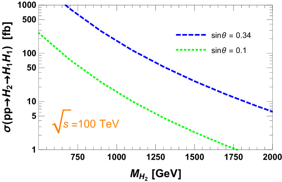
Figure 11: Production cross section of $pp\to H_{2}\to H_{1}H_{1}$ vs mass of $H_{2}$ for different values of the Higgs mixing angle.

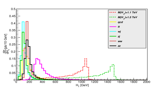
Figure 12: $H_{T}$ distribution for signal and background samples.

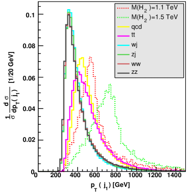
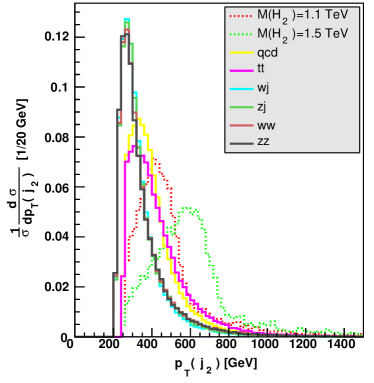
Figure 13: $p_{T}$ distribution of leading fatjet $j_{1}$ (Left panel) and sub-leading fatjet $j_{2}$ (Right panel). We also show the $p_{T}$ distributions of the fatjets arising from background samples.

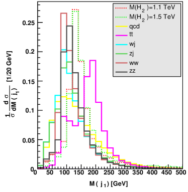
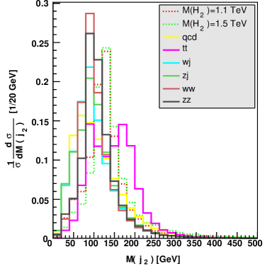
Figure 14: Left panel: invariant mass distribution of the leading fatjet $j_{1}$. Right panel: the same for the sub-leading fatjet $j_{2}$.

In Fig. 11, we show the production cross section of $pp\to H_{2}\to H_{1}H_{1}$ at $\sqrt{s}=100$ TeV as a function of the mass of $H_{2}$ for $\sin\theta=0.1,\ 0.34$. There are a number of SM backgrounds, that can mimic the signal. This include both QCD and electroweak processes. The QCD is generated by combining $b\bar{b}b\bar{b}$ and $b\bar{b}jj$ final state. The other backgrounds which includes electroweak coupling are di-top ($t\bar{t}$), di-boson ($WW\text{ and }ZZ$), $Wj$ and $Zj$. Here we consider full hadronic decays of top quark, $W$ and $Z$ boson. At the generator level, we implement these following cuts on background samples:

• The transverse momentum of the partons: $p_{T}^{j}>20\,\textrm{GeV}$, $p_{T}^{b}>15\,\textrm{GeV}$

• The pseudo-rapidity of the partons: $|\eta_{j}|<5.0$, $|\eta_{b}|<3.0$

• The separation between partons: $\Delta R_{jj}>0.4$, $\Delta R_{bb}>0.2$, $\Delta R_{bj}>0.4$

• Invariant mass of the two $b$ quark: $m_{bb}>30\,\textrm{GeV}$

• The scalar sum of the transverse momentum of all the hadronic particles $H_{T}$ of the background: $H_{T}>800\,\textrm{GeV}$

The third cut on $\Delta R$ is to avoid any divergence, that may arise from the QCD samples. The distribution of $H_{T}$ is shown in Fig. 12. The cut on $H_{T}$ ensures the sufficiently large background population in the desired region, where signal populates. We do not consider the SM di-Higgs channel into consideration, as we find that after the $H_{T}$ cut, the di-Higgs channel including $h\to b\bar{b}$ branching ratio only gives $\sigma<2.5\,\textrm{ fb}$ cross-section, which is suppressed compared to other backgrounds. The signal as compared to background shows distinct features in the distributions of different kinematic variables. In Fig. 13, we show $p_{T}$ distributions of the two fatjets, for two mass points of the BSM Higgs $M_{H_{2}}=1.1,1.5$ TeV. As clearly seen in the figure the $p_{T}$ distributions of the two leading jets for the signal and backgrounds are not very much well separated. The peak of the $p_{T}$ distributions for the first and the second jets occurs at a relatively higher values of $p_{T}$ as compared to the background. Therefore, to reduce the background without affecting the signal we demand a higher values of $p_{T}$ on leading and sub-leading fatjets as cut, which are $p_{T}(j_{1})>250$ GeV and $p_{T}(j_{2})>250$ GeV.

In Fig. 14, the leading and sub-leading fatjet masses have been displayed. For the signal the two jets are produced from the decay of the SM-like Higgs, hence the peaks for the distribution of $M(j_{1})$ and $M({j_{2}})$ occur around the Higgs mass ($M_{H_{1}}\sim 125$ GeV). Since these fatjets are formed after showering and hadronization of $b\bar{b}$ pair, therefore we expect a non-trivial two prong substructure inside each of the fatjets. We use Soft Drop algorithm Larkoski:2014wba which uses the condition $\frac{min(p_{T}(subjet1),p_{T}(subjet2))}{(p_{T}(subjet1)+p_{T}(subjet1))}>0.1$ to determine whether subjets are created from Higgs decays. All subjets which satisfy this condition are qualified as the subjets originating from Higgs decay. In Delphes a subjet can not be tagged as $b$-jet. We implement a naive $b$-jet tagging for subjets in our analysis. We use $B$-hadron to tag the subjet originating from $b$ quark. We consider $b$-tag efficiency for the subjet is $80\%$ with mis-tag efficiency $1\%$. In Fig. 15, we show the invariant mass distribution of the fatjet pairs, the signal peaks around $M_{H_{2}}$. We use these features to reduce the backgrounds while not reducing too much the signal.

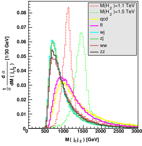
Figure 15: Invariant mass distribution of the fatjet pair.

Therefore our selection cuts are the following:

• $c_{1}$ : We demand at least two fatjets in the final state, $N_{j}\geq 2$.

• $c_{2}$: Bound on the leading and sub-leading fatjets $p_{T}$ are $p_{T}(j_{1})\geq 250$ GeV and $p_{T}(j_{2})\geq 250$ GeV.

• $c_{3}$ : The mass of leading and sub-leading fatjet must be within 20 GeV of the SM Higgs mass, $|M_{H_{1}}-M_{j_{1,2}}|\leq 20$ GeV.

• $c_{4}$ : The invariant mass of the two fatjets will deviate at most by 150 GeV from the BSM Higgs mass, $|M_{H_{2}}-M(j_{1}j_{2})|\leq 150$.

• $c_{5}$: Pseudo-rapidity separation between $j_{1}$ and $j_{2}$, $|\Delta\eta(j_{1}j_{2})|\leq 1.5$.

• $c_{6}$ : The leading and sub-leading fatjets must contain at least two subjets.

• $c_{7}$ : For the leading and sub-leading fatjets, each of the fatjets will contain two $b$-tagged subjets.

We show the partonic cross-sections of different SM backgrounds in Table. 4. As can be seen, the main background is QCD, with a cross-section $\sigma_{QCD}\sim 10^{7}$ fb at the partonic level. The other backgrounds, such as $t\bar{t},Wj,Zj$ have a cross-section $\sigma\sim 10^{4}$ fb. In the third and fourth column, we show the cross-sections of the backgrounds after implementing all the cuts $c_{1}-c_{7}$.

We also checked that for a resolved analysis with standard set of cuts, a) number of $b$ jet $\geq 4$, b) $p_{T}(b)>30$ GeV, c) invariant mass of Higgs $m_{bb}=125\pm 20$ GeV, d) $b$ tagging efficiency same as the fatjet analysis, and e) invariant mass of 4$b$ jet similar to the fatjet analysis, the QCD cross-section is large $\sigma=4878$ fb (2795 fb) for $M_{H_{2}}=1.1$ TeV (1.5 TeV). For the resolved analysis, additional background contributions such as $W+2j,\,Z+2j,\,jbb,$ and others are also relevant.

BG	$\sigma^{partonic}$ [fb]	$\sigma^{analysis}$ [fb] ($950<M(j_{1}j_{2})<1250$)	$\sigma^{analysis}$ [fb] ($1350<M(j_{1}j_{2})<1650$)
$QCD$	$4.1479\times 10^{7}$	$1789.9$	$211$
$t\bar{t}$	$7.603\times 10^{4}$	$0.03$	$9.9\times 10^{-5}$
$Wj$	$5.311\times 10^{4}$	$0.0018$	$0.43$
$Zj$	$5.89\times 10^{4}$	$1.9$	$0.006$
$WW$	$1.2815\times 10^{2}$	$2\times 10^{-6}$	$3\times 10^{-7}$
$ZZ$	$3.614\times 10^{1}$	$1.3\times 10^{-6}$	$5\times 10^{-8}$

Table 4: Background cross section before and after the cuts.

	$M_{H_{2}}$=1.1 TeV		$M_{H_{2}}$=1.5 TeV
	$\sigma^{s}$ [fb]	$\sigma^{b}$ [fb]	$\sigma^{s}$ [fb]	$\sigma^{b}$ [fb]
before cut	$36.22\ (3.13)$	$4.17\times 10^{7}$	$8.64\ (0.75)$	$4.17\times 10^{7}$
after cut	$0.745\ (0.064)$	$1791.9$	$0.19\ (0.016)$	$211.43$
$\frac{\sigma^{s}\sqrt{\mathcal{L}}}{\sqrt{\sigma^{s}+\sigma^{b}}}$, $\mathcal{L}=30\ \text{ab}^{-1}$	$\qquad 3.05\ (0.26)\qquad$		$\qquad 2.26\ (0.19)\qquad$

Table 5: Signal ($pp\to 2j_{\textrm{fat}}$) and background cross-sections after different selection cuts at $\sqrt{s}=100$ TeV for $\sin\theta=0.34\ (0.1)$.

In Table 5, we show the signal cross-sections before and after applying the cuts $c_{1}-c_{7}$. We consider two illustrative BSM Higgs masses $M_{H_{2}}=1.1,1.5$ TeV. The background in this table corresponds to the QCD background, shown in Table. 4, as this is the major background. As can be seen from the table the background is huge as compared to the signal. Applying the cuts however allows to improve the significance of the signal. The main remaining background is $QCD$. We find that for $M_{H_{2}}$=1.1 TeV , one can achieve $3\sigma$ significance of the signal over background for 30 $ab^{-1}$ luminosity. For higher mass values of the BSM Higgs, significance reduces. The significance of the signal can be improved over the background if one uses multivariate analysis and neural network methods. Additional final states such as $b\bar{b}\gamma\gamma$/ $b\bar{b}\tau^{+}\tau^{-}$ are expected to give better significance, as these are clean channels. Detailed evaluation of the discovery prospect of all these channels is beyond the scope of this paper, and we will present this elsewhere.

5 Conclusion

In this work, we adopt an effective field theory framework that contains RHN and one SM gauge singlet scalar. Our model accommodates a FIMP DM candidate and explains the observed eV masses of light neutrinos, where SM neutrinos acquire their masses via seesaw mechanism. Three gauge singlet RHN states $N_{1,2,3}$ and one gauge singlet real scalar $\chi$ are present in addition to the SM fields. The two RHN states $N_{1,2}$ participate in light neutrino mass generation and $N_{3}$ is the DM. There is sizeable mixing between the BSM scalar and the SM Higgs, that offers better detection prospect of the BSM Higgs at colliders.

The FIMP DM candidate $N_{3}$ in our model interacts with the SM and BSM scalars only via effective $d=5$ Yukawa interaction. The $d=5$ term generates the tri-linear interaction term responsible for decay once $\chi$ and $\Phi$ acquire vev. Hence FIMP DM can be produced from the decay of the SM and BSM Higgs. Annihilation of scalars and other SM particles can also lead to DM production. However, for a low reheating temperature, the decay contribution dominates. In our analysis, we therefore first consider a low reheating temperature and analyse only decay contributions. In Scenario-I and II, where there is no bare-mass term of $N_{1,2,3}$ being added, both the DM mass and its interaction with other particles depend on the same operator. Therefore, the relic density constraint leads to a strong correlation between the vev of BSM scalar ($v_{\chi}$) and mass of DM ($M_{N_{3}}$). Keeping other parameters fixed, the required value of $v_{\chi}$ to satisfy the observed relic density increases with the mass of DM. The same $v_{\chi}$ also primarily governs the BSM Higgs mass $M_{H_{2}}$. Since in our model SM and BSM Higgs mixing can be sizeable, a TeV scale or lighter $H_{2}$ therefore has better discovery prospect at collider as compared to a very heavy $H_{2}$. We find that, for TeV scale $v_{\chi}$ which is a natural choice for TeV scale or lower BSM Higgs state, DM relic density constraint is satisfied only if its mass is in the KeV range. We also consider another scenario Scenario-III, where we accommodate a bare mass term of the RHN states. We find that in this case, the tight correlation between vev of $\chi$ and mass of DM is somewhat relaxed, and a GeV scale DM is possible to accommodate with a TeV scale BSM Higgs/vev $v_{\chi}$.

We also consider a variation of the reheating temperature $T_{R}$ and study the different annihilation channels. For a high reheating temperature we consider both the decay and annihilation contributions in relic density, where the latter dominates the relic abundance. A number of annihilation channels $WW/ZZ/H_{i}H_{i}\to N_{3}N_{3}$ can give significant contributions. In our analysis, we show the variation of relic density w.r.t various parameters, such as $v_{\chi}$, mass of DM, and reheating temperature. We find that the relic density increases with the mass of DM, and $T_{R}$ (for gauge boson and scalar annihilation only), and decreases for higher vev of BSM scalar. Assuming BSM Higgs varying in $\mathcal{O}(\textrm{TeV})$ range, we vary these parameters in a wide range and show the variation of relic density as scatter plot.

Finally, we explore the collider signature of the TeV scale BSM scalar at the 100 TeV future $pp$ machine. We consider the production of the BSM scalar which has sizeable mixing with the SM Higgs, and its decay to a pair of SM Higgs states. We further consider the decay of the SM Higgs to $b\bar{b}$ states. For a TeV scale heavy Higgs, the SM Higgs is rather moderately boosted leading to collimated decay products. We consider di-fatjet final states as our model signature. We perform a detailed analysis considering several backgrounds, such as, QCD, $t\bar{t}$, $WW/ZZ,W+1j,Z+1j$. Following a cut based analysis we find that a $3\sigma$ significance can be achieved for a 1.1 TeV BSM scalar with $30\text{ ab}^{-1}$ luminosity. Thus, the di-fatjet channel which is sensitive to the tri-linear Higgs coupling $H_{2}H_{1}H_{1}$ is a complementary probe for the heavy BSM Higgs, in addition to other channels, such as $pp\to H_{2}\to WW/ZZ$.

Appendix

In this section, we discuss various expressions of the annihilation contributions to relic density.

Analytical expression of relevant cross sections

We list the cross-sections for the $AB\rightarrow N_{3}N_{3}$ processes where $A$, $B$ are any SM particles contributing to DM production in the freeze-in mechanism.

• $WW\rightarrow N_{3}N_{3}$:

  $$g_{H_{1}W^{+}W^{-}} = \frac{M_{W}e\cos\theta}{s_{w}}\,,$$

  $$g_{H_{2}W^{+}W^{-}} = \frac{M_{W}e\sin\theta}{s_{w}},$$

  $$A_{WW} = \dfrac{g_{H_{1}W^{+}W^{-}}\,\,g_{H_{1}N_{3}N_{3}}}{(s-M_{H_{1}}^{2})+iM_{H_{1}}\Gamma_{H_{1}}}+\dfrac{g_{H_{2}W^{+}W^{-}}\,g_{H_{2}N_{3}N_{3}}}{(s-M_{H_{2}}^{2})+iM_{H_{2}}\Gamma_{H_{2}}},$$

  $$M_{WW} = \dfrac{2}{9}\,\left(1+\dfrac{(s-2M_{W}^{2})^{2}}{8M_{W}^{4}}\right)\,\,\left(s-4M^{2}_{N_{3}}\right)\,|A_{WW}|^{2},$$

  $$\sigma_{WW\rightarrow N_{3}N_{3}} = \dfrac{1}{16\pi s}\,\,\sqrt{\dfrac{s-4M_{N_{3}}^{2}}{s-4M_{W}^{2}}}\,\,\,M_{WW}\,.$$ (68)

• $ZZ\rightarrow N_{3}N_{3}$:

  $$g_{H_{1}ZZ} = \frac{M_{W}e\cos\theta}{c^{2}_{w}s_{w}}\,,$$

  $$g_{H_{2}ZZ} = \frac{M_{W}e\sin\theta}{c^{2}_{w}s_{w}},$$

  $$A_{ZZ} = \dfrac{g_{H_{1}ZZ}\,\,g_{H_{1}N_{3}N_{3}}}{(s-M_{H_{1}}^{2})+iM_{H_{1}}\Gamma_{H_{1}}}+\dfrac{g_{H_{2}ZZ}\,g_{H_{2}N_{3}N_{3}}}{(s-M_{H_{2}}^{2})+iM_{H_{2}}\Gamma_{H_{2}}},$$

  $$M_{ZZ} = \dfrac{2}{9}\,\left(1+\dfrac{(s-2M_{W}^{2})^{2}}{8M_{W}^{4}}\right)\,\,\left(s-4M^{2}_{N_{3}}\right)\,|A_{ZZ}|^{2},$$

  $$\sigma_{ZZ\rightarrow N_{3}N_{3}} = \dfrac{1}{32\pi s}\,\,\sqrt{\dfrac{s-4M_{N_{3}}^{2}}{s-4M_{Z}^{2}}}\,\,\,M_{ZZ}\,.$$ (69)

• $f\bar{f}\rightarrow N_{3}N_{3}$:

  $$g_{H_{1}ff} = -\frac{eM_{f}\cos\theta}{2M_{W}}\,,$$

  $$g_{H_{2}ff} = -\frac{eM_{f}\sin\theta}{2M_{W}},$$

  $$A_{ff} = \dfrac{g_{H_{1}ff}\,\,g_{H_{1}N_{3}N_{3}}}{(s-M_{H_{1}}^{2})+iM_{H_{1}}\Gamma_{H_{1}}}+\dfrac{g_{H_{2}ff}\,g_{H_{2}N_{3}N_{3}}}{(s-M_{H_{2}}^{2})+iM_{H_{2}}\Gamma_{H_{2}}},$$

  $$M_{ff} = \dfrac{2}{n_{c}}\,\left(s-4M^{2}_{f}\right)\,\,\left(s-4M^{2}_{N_{3}}\right)\,|A_{ff}|^{2},$$

  $$\sigma_{f\bar{f}\rightarrow N_{3}N_{3}} = \dfrac{1}{64\pi s}\,\,\sqrt{\dfrac{s-4M_{N_{3}}^{2}}{s-4M_{f}^{2}}}\,\,\,M_{ff}\,.$$ (70)

• $H_{i}H_{j}\rightarrow N_{3}N_{3}\,\,(i,j=1,2)$:

  $$g_{H_{1}H_{1}H_{1}}=-3\,[2\,v\lambda_{H_{1}}\cos^{3}\theta+2\,v_{\chi}\,\lambda_{H_{2}}\sin^{3}\theta+\lambda_{H_{1}H_{2}}\sin\theta\,\cos\theta\,(v\sin\theta+v_{\chi}\cos\theta)],$$

  $$g_{H_{1}H_{1}H_{2}}=[6\,v\lambda_{H_{1}}\cos^{2}\theta\sin\theta-6\,v_{\chi}\lambda_{H_{2}}\sin^{2}\theta\,\cos\theta-(2-3\,\sin^{2}\theta)\,v\,\lambda_{H_{1}H_{2}}\,\sin\theta$$

  $$~{}~{}~{}~{}~{}~{}~{}~{}~{}-(1-3\sin^{2}\theta)v_{\chi}\,\lambda_{H_{1}H_{2}}\cos\theta]\,,$$ (71)

  $$g_{H_{2}H_{2}H_{2}}=3\,[2\,v\lambda_{H_{1}}\sin^{3}\theta-2\,v_{\chi}\lambda_{H_{2}}\cos^{3}\theta+\lambda_{H_{1}H_{2}}\sin\theta\cos\theta\,(v\cos\theta-v_{\chi}\sin\theta)],$$

  $$g_{H_{2}H_{2}H_{1}}=-[6\,v\lambda_{H_{1}}\sin^{2}\theta\cos\theta+6\,v_{\chi}\lambda_{H_{2}}\cos^{2}\theta\sin\theta-(2-3\,\sin^{2}\theta)v_{\chi}\lambda_{H_{1}H_{2}}\sin\theta\,\,$$

  $$~{}~{}~{}~{}~{}~{}~{}~{}~{}+(1-3\sin^{2}\theta)v\lambda_{H_{1}H_{2}}\cos\theta]\,,$$

  $$g_{H_{1}H_{1}N_{3}N_{3}}=(\frac{c^{\prime}_{33}}{\Lambda}\cos^{2}\theta+\frac{c_{33}}{\Lambda}\sin^{2})\,,$$

  $$g_{H_{2}H_{2}N_{3}N_{3}}=(\frac{c^{\prime}_{33}}{\Lambda}\sin^{2}\theta+\frac{c_{33}}{\Lambda}\cos^{2}\theta)$$

  $$g_{H_{1}H_{2}N_{3}N_{3}}=\sin\alpha\cos\alpha(\frac{c^{\prime}_{33}}{\Lambda}-\frac{c_{33}}{\Lambda})\,,$$

  $$M_{H_{i}H_{j}}=\dfrac{g_{H_{i}H_{j}H_{1}}\,\,g_{H_{1}N_{3}N_{3}}}{(s-M_{H_{1}}^{2})+iM_{H_{1}}\Gamma_{H_{1}}}+\dfrac{g_{H_{i}H_{j}H_{2}}\,\,g_{H_{2}N_{3}N_{3}}}{(s-M_{H_{2}}^{2})+iM_{H_{2}}\Gamma_{H_{2}}}+g_{H_{i}H_{j}N_{3}N_{3}},$$

  $$\sigma_{H_{i}H_{j}\rightarrow N_{3}N_{3}}=\dfrac{1}{16\pi s}\,\,\sqrt{\dfrac{s(s-4M_{N_{3}}^{2})}{(s-(M_{H_{i}}+M_{H_{j}})^{2})(s-(M_{H_{i}}-M_{H_{j}})^{2})}}\,\,\,|M_{H_{i}H_{j}}|^{2}\,.$$ (72)

As given in Hall:2009bx , we can approximately calculate the DM contribution analytically for higher value of the reheating temperature by solving the following Boltzmann equation,

$$\frac{dn_{N_{3}}}{dt}+3n_{N_{3}}H\simeq\frac{T}{1024}\int dsd\Omega\sqrt{s}|M|^{2}_{AB\rightarrow N_{3}N_{3}}K_{1}\left(\frac{\sqrt{s}}{T}\right)\,.$$ (73)

We parametrise the amplitude for the $A\,B\rightarrow N_{3}N_{3}$ process to be proportional to some power of centre of mass energy at very high temperature i.e. $|M|^{2}_{AB\rightarrow N_{3}N_{3}}=\alpha s^{n}$ where $\alpha$ is a constant which depends on the couplings and $n$ is a rational number. After substituting the above amplitude and focusing on the dependence of the co-moving number density on temperature, we obtain

$$\frac{dY_{UV}}{dT}=\kappa T^{2n-2}$$ (74)

where $Y_{UV}$ is the co-moving number density of DM and $\kappa$ is a constant. In the present work the amplitude varies in the following way at large $s$,

$$|M|^{2} = \alpha_{AB}s\,\,\,{\rm where}\,\,\,A,B\,\,=\,\,W,Z,H_{1},H_{2}$$ (75)

$$= \alpha_{ff}\,\,\,{\rm where}\,\,\,{f\,\,is\,\,\rm SM\,\,\rm fermion}\,.$$

Therefore, for gauge bosons and Higgses we can easily show that,

$$Y_{UV}=\kappa T_{R}$$ (76)

and for the fermion it will be

$$Y_{UV}=\kappa(\frac{1}{T_{0}}-\frac{1}{T_{R}})\,.$$ (77)

Finally, we can conclude that for the Higgs bosons and gauge boson the relic density contribution increase linearly with $T_{R}$, whereas for fermions the contribution does not change significantly with the $T_{R}$ for high value of $T_{R}$.

References

- (1) Z. Maki, M. Nakagawa, and S. Sakata, “Remarks on the unified model of elementary particles,” Prog. Theor. Phys. 28 (1962) 870–880.
- (2) B. Pontecorvo, “Neutrino Experiments and the Problem of Conservation of Leptonic Charge,” Sov. Phys. JETP 26 (1968) 984–988.
- (3) I. Esteban, M. C. Gonzalez-Garcia, M. Maltoni, T. Schwetz, and A. Zhou, “The fate of hints: updated global analysis of three-flavor neutrino oscillations,” JHEP 09 (2020) 178, arXiv:2007.14792 [hep-ph].
- (4) S. Weinberg, “Baryon and Lepton Nonconserving Processes,” Phys. Rev. Lett. 43 (1979) 1566–1570.
- (5) F. Wilczek and A. Zee, “Operator Analysis of Nucleon Decay,” Phys. Rev. Lett. 43 (1979) 1571–1573.
- (6) P. Minkowski, “ at a Rate of One Out of Muon Decays?,” Phys. Lett. B67 (1977) 421–428.
- (7) R. N. Mohapatra and G. Senjanovic, “Neutrino Mass and Spontaneous Parity Violation,” Phys. Rev. Lett. 44 (1980) 912.
- (8) T. Yanagida, “Horizontal Symmetry and Masses of Neutrinos,” Conf. Proc. C7902131 (1979) 95–99.
- (9) M. Gell-Mann, P. Ramond, and R. Slansky, “Complex Spinors and Unified Theories,” Conf. Proc. C790927 (1979) 315–321, arXiv:1306.4669 [hep-th].
- (10) Y. G. Kim and K. Y. Lee, “The Minimal model of fermionic dark matter,” Phys. Rev. D 75 (2007) 115012, arXiv:hep-ph/0611069.
- (11) Y. G. Kim, K. Y. Lee, and S. Shin, “Singlet fermionic dark matter,” JHEP 05 (2008) 100, arXiv:0803.2932 [hep-ph].
- (12) L. Lopez-Honorez, T. Schwetz, and J. Zupan, “Higgs portal, fermionic dark matter, and a Standard Model like Higgs at 125 GeV,” Phys. Lett. B 716 (2012) 179–185, arXiv:1203.2064 [hep-ph].
- (13) L. J. Hall, K. Jedamzik, J. March-Russell, and S. M. West, “Freeze-In Production of FIMP Dark Matter,” JHEP 03 (2010) 080, arXiv:0911.1120 [hep-ph].
- (14) J. McDonald, “Thermally generated gauge singlet scalars as selfinteracting dark matter,” Phys. Rev. Lett. 88 (2002) 091304, arXiv:hep-ph/0106249.
- (15) A. Biswas and A. Gupta, “Freeze-in Production of Sterile Neutrino Dark Matter in U(1)B-L Model,” JCAP 09 (2016) 044, arXiv:1607.01469 [hep-ph]. [Addendum: JCAP 05, A01 (2017)].
- (16) P. Bandyopadhyay, M. Mitra, and A. Roy, “Relativistic Freeze-in with Scalar Dark Matter in a Gauged Model and Electroweak Symmetry Breaking,” arXiv:2012.07142 [hep-ph].
- (17) F. Elahi, C. Kolda, and J. Unwin, “UltraViolet Freeze-in,” JHEP 03 (2015) 048, arXiv:1410.6157 [hep-ph].
- (18) S.-L. Chen and Z. Kang, “On UltraViolet Freeze-in Dark Matter during Reheating,” JCAP 05 (2018) 036, arXiv:1711.02556 [hep-ph].
- (19) A. Biswas, S. Ganguly, and S. Roy, “Fermionic dark matter via UV and IR freeze-in and its possible X-ray signature,” JCAP 03 (2020) 043, arXiv:1907.07973 [hep-ph].
- (20) N. Bernal, J. Rubio, and H. Veermäe, “Boosting Ultraviolet Freeze-in in NO Models,” JCAP 06 (2020) 047, arXiv:2004.13706 [hep-ph].
- (21) S. Bhattacharya and J. Wudka, “Effective Theories with Dark Matter Applications,” arXiv:2104.01788 [hep-ph].
- (22) B. Barman, D. Borah, and R. Roshan, “Effective Theory of Freeze-in Dark Matter,” JCAP 11 (2020) 021, arXiv:2007.08768 [hep-ph].
- (23) R. T. Co, F. D’Eramo, L. J. Hall, and D. Pappadopulo, “Freeze-In Dark Matter with Displaced Signatures at Colliders,” JCAP 12 (2015) 024, arXiv:1506.07532 [hep-ph].
- (24) G. Bélanger et al., “LHC-friendly minimal freeze-in models,” JHEP 02 (2019) 186, arXiv:1811.05478 [hep-ph].
- (25) L. Calibbi, F. D’Eramo, S. Junius, L. Lopez-Honorez, and A. Mariotti, “Displaced new physics at colliders and the early universe before its first second,” arXiv:2102.06221 [hep-ph].
- (26) J. M. No, P. Tunney, and B. Zaldivar, “Probing Dark Matter freeze-in with long-lived particle signatures: MATHUSLA, HL-LHC and FCC-hh,” JHEP 03 (2020) 022, arXiv:1908.11387 [hep-ph].
- (27) G. Bélanger, C. Delaunay, A. Pukhov, and B. Zaldivar, “Dark matter abundance from the sequential freeze-in mechanism,” Phys. Rev. D 102 no. 3, (2020) 035017, arXiv:2005.06294 [hep-ph].
- (28) E. Molinaro, C. E. Yaguna, and O. Zapata, “FIMP realization of the scotogenic model,” JCAP 07 (2014) 015, arXiv:1405.1259 [hep-ph].
- (29) G. Bélanger, F. Boudjema, A. Goudelis, A. Pukhov, and B. Zaldivar, “micrOMEGAs5.0 : Freeze-in,” Comput. Phys. Commun. 231 (2018) 173–186, arXiv:1801.03509 [hep-ph].
- (30) C. P. Burgess, M. Pospelov, and T. ter Veldhuis, “The Minimal model of nonbaryonic dark matter: A Singlet scalar,” Nucl. Phys. B 619 (2001) 709–728, arXiv:hep-ph/0011335.
- (31) V. Barger, P. Langacker, M. McCaskey, M. J. Ramsey-Musolf, and G. Shaughnessy, “LHC Phenomenology of an Extended Standard Model with a Real Scalar Singlet,” Phys. Rev. D 77 (2008) 035005, arXiv:0706.4311 [hep-ph].
- (32) CMS Collaboration, A. M. Sirunyan et al., “Combined measurements of Higgs boson couplings in proton–proton collisions at ,” Eur. Phys. J. C 79 no. 5, (2019) 421, arXiv:1809.10733 [hep-ex].
- (33) Planck Collaboration, N. Aghanim et al., “Planck 2018 results. VI. Cosmological parameters,” Astron. Astrophys. 641 (2020) A6, arXiv:1807.06209 [astro-ph.CO].
- (34) P. Gondolo and G. Gelmini, “Cosmic abundances of stable particles: Improved analysis,” Nucl. Phys. B 360 (1991) 145–179.
- (35) A. Alloul, N. D. Christensen, C. Degrande, C. Duhr, and B. Fuks, “FeynRules 2.0 - A complete toolbox for tree-level phenomenology,” Comput. Phys. Commun. 185 (2014) 2250–2300, arXiv:1310.1921 [hep-ph].
- (36) ATLAS Collaboration, G. Aad et al., “Search for heavy resonances decaying into a pair of bosons in the and final states using 139 fb-1 of proton-proton collisions at TeV with the ATLAS detector,” arXiv:2009.14791 [hep-ex].
- (37) ATLAS Collaboration, G. Aad et al., “Search for heavy diboson resonances in semileptonic final states in collisions at TeV with the ATLAS detector,” Eur. Phys. J. C 80 no. 12, (2020) 1165, arXiv:2004.14636 [hep-ex].
- (38) ATLAS Collaboration, G. Aad et al., “Combination of searches for Higgs boson pairs in collisions at 13 TeV with the ATLAS detector,” Phys. Lett. B 800 (2020) 135103, arXiv:1906.02025 [hep-ex].
- (39) ATLAS Collaboration, G. Aad et al., “Search for the process via vector-boson fusion production using proton-proton collisions at TeV with the ATLAS detector,” JHEP 07 (2020) 108, arXiv:2001.05178 [hep-ex]. [Erratum: JHEP 01, 145 (2021)].
- (40) CMS Collaboration, A. M. Sirunyan et al., “Search for resonant pair production of Higgs bosons decaying to bottom quark-antiquark pairs in proton-proton collisions at 13 TeV,” JHEP 08 (2018) 152, arXiv:1806.03548 [hep-ex].
- (41) P. Bechtle, D. Dercks, S. Heinemeyer, T. Klingl, T. Stefaniak, G. Weiglein, and J. Wittbrodt, “HiggsBounds-5: Testing Higgs Sectors in the LHC 13 TeV Era,” Eur. Phys. J. C 80 no. 12, (2020) 1211, arXiv:2006.06007 [hep-ph].
- (42) U. Baur, T. Plehn, and D. L. Rainwater, “Determining the Higgs Boson Selfcoupling at Hadron Colliders,” Phys. Rev. D 67 (2003) 033003, arXiv:hep-ph/0211224.
- (43) U. Baur, T. Plehn, and D. L. Rainwater, “Probing the Higgs selfcoupling at hadron colliders using rare decays,” Phys. Rev. D 69 (2004) 053004, arXiv:hep-ph/0310056.
- (44) A. Azatov, R. Contino, G. Panico, and M. Son, “Effective field theory analysis of double Higgs boson production via gluon fusion,” Phys. Rev. D 92 no. 3, (2015) 035001, arXiv:1502.00539 [hep-ph].
- (45) F. Kling, T. Plehn, and P. Schichtel, “Maximizing the significance in Higgs boson pair analyses,” Phys. Rev. D 95 no. 3, (2017) 035026, arXiv:1607.07441 [hep-ph].
- (46) M. J. Dolan, C. Englert, and M. Spannowsky, “Higgs self-coupling measurements at the LHC,” JHEP 10 (2012) 112, arXiv:1206.5001 [hep-ph].
- (47) A. Papaefstathiou, L. L. Yang, and J. Zurita, “Higgs boson pair production at the LHC in the channel,” Phys. Rev. D 87 no. 1, (2013) 011301, arXiv:1209.1489 [hep-ph].
- (48) A. J. Barr, M. J. Dolan, C. Englert, and M. Spannowsky, “Di-Higgs final states augMT2ed – selecting events at the high luminosity LHC,” Phys. Lett. B 728 (2014) 308–313, arXiv:1309.6318 [hep-ph].
- (49) S. Banerjee, C. Englert, M. L. Mangano, M. Selvaggi, and M. Spannowsky, “ production at 100 TeV,” Eur. Phys. J. C 78 no. 4, (2018) 322, arXiv:1802.01607 [hep-ph].
- (50) D. E. Ferreira de Lima, A. Papaefstathiou, and M. Spannowsky, “Standard model Higgs boson pair production in the final state,” JHEP 08 (2014) 030, arXiv:1404.7139 [hep-ph].
- (51) D. Wardrope, E. Jansen, N. Konstantinidis, B. Cooper, R. Falla, and N. Norjoharuddeen, “Non-resonant Higgs-pair production in the final state at the LHC,” Eur. Phys. J. C 75 no. 5, (2015) 219, arXiv:1410.2794 [hep-ph].
- (52) J. K. Behr, D. Bortoletto, J. A. Frost, N. P. Hartland, C. Issever, and J. Rojo, “Boosting Higgs pair production in the final state with multivariate techniques,” Eur. Phys. J. C 76 no. 7, (2016) 386, arXiv:1512.08928 [hep-ph].
- (53) S. Banerjee, B. Batell, and M. Spannowsky, “Invisible decays in Higgs boson pair production,” Phys. Rev. D 95 no. 3, (2017) 035009, arXiv:1608.08601 [hep-ph].
- (54) M. J. Dolan, C. Englert, and M. Spannowsky, “New Physics in LHC Higgs boson pair production,” Phys. Rev. D 87 no. 5, (2013) 055002, arXiv:1210.8166 [hep-ph].
- (55) J. M. No and M. Ramsey-Musolf, “Probing the Higgs Portal at the LHC Through Resonant di-Higgs Production,” Phys. Rev. D 89 no. 9, (2014) 095031, arXiv:1310.6035 [hep-ph].
- (56) V. Martín Lozano, J. M. Moreno, and C. B. Park, “Resonant Higgs boson pair production in the decay channel,” JHEP 08 (2015) 004, arXiv:1501.03799 [hep-ph].
- (57) T. Huang, J. No, L. Pernié, M. Ramsey-Musolf, A. Safonov, M. Spannowsky, and P. Winslow, “Resonant di-Higgs boson production in the channel: Probing the electroweak phase transition at the LHC,” Phys. Rev. D 96 no. 3, (2017) 035007, arXiv:1701.04442 [hep-ph].
- (58) J. Ren, R.-Q. Xiao, M. Zhou, Y. Fang, H.-J. He, and W. Yao, “LHC Search of New Higgs Boson via Resonant Di-Higgs Production with Decays into 4W,” JHEP 06 (2018) 090, arXiv:1706.05980 [hep-ph].
- (59) P. Basler, S. Dawson, C. Englert, and M. Mühlleitner, “Di-Higgs boson peaks and top valleys: Interference effects in Higgs sector extensions,” Phys. Rev. D 101 no. 1, (2020) 015019, arXiv:1909.09987 [hep-ph].
- (60) H.-L. Li, M. Ramsey-Musolf, and S. Willocq, “Probing a scalar singlet-catalyzed electroweak phase transition with resonant di-Higgs boson production in the channel,” Phys. Rev. D 100 no. 7, (2019) 075035, arXiv:1906.05289 [hep-ph].
- (61) A. Adhikary, S. Banerjee, R. Kumar Barman, and B. Bhattacherjee, “Resonant heavy Higgs searches at the HL-LHC,” JHEP 09 (2019) 068, arXiv:1812.05640 [hep-ph].
- (62) L.-C. Lü, C. Du, Y. Fang, H.-J. He, and H. Zhang, “Searching heavier Higgs boson via di-Higgs production at LHC Run-2,” Phys. Lett. B 755 (2016) 509–522, arXiv:1507.02644 [hep-ph].
- (63) A. Alves, D. Gonçalves, T. Ghosh, H.-K. Guo, and K. Sinha, “Di-Higgs Production in the Channel and Gravitational Wave Complementarity,” JHEP 03 (2020) 053, arXiv:1909.05268 [hep-ph].
- (64) ATLAS Collaboration, M. Aaboud et al., “Search for pair production of Higgs bosons in the final state using proton–proton collisions at TeV with the ATLAS detector,” Phys. Rev. D 94 no. 5, (2016) 052002, arXiv:1606.04782 [hep-ex].
- (65) CMS Collaboration, V. Khachatryan et al., “Search for heavy resonances decaying to two Higgs bosons in final states containing four b quarks,” Eur. Phys. J. C 76 no. 7, (2016) 371, arXiv:1602.08762 [hep-ex].
- (66) CMS Collaboration, V. Khachatryan et al., “Search for two Higgs bosons in final states containing two photons and two bottom quarks in proton-proton collisions at 8 TeV,” Phys. Rev. D 94 no. 5, (2016) 052012, arXiv:1603.06896 [hep-ex].
- (67) ATLAS Collaboration, G. Aad et al., “Searches for Higgs boson pair production in the channels with the ATLAS detector,” Phys. Rev. D 92 (2015) 092004, arXiv:1509.04670 [hep-ex].
- (68) ATLAS Collaboration, M. Aaboud et al., “Search for pair production of Higgs bosons in the final state using proton-proton collisions at TeV with the ATLAS detector,” JHEP 01 (2019) 030, arXiv:1804.06174 [hep-ex].
- (69) ATLAS Collaboration, M. Aaboud et al., “Search for Higgs boson pair production in the decay mode at TeV with the ATLAS detector,” JHEP 04 (2019) 092, arXiv:1811.04671 [hep-ex].
- (70) ATLAS Collaboration, M. Aaboud et al., “Search for resonant and non-resonant Higgs boson pair production in the decay channel in collisions at TeV with the ATLAS detector,” Phys. Rev. Lett. 121 no. 19, (2018) 191801, arXiv:1808.00336 [hep-ex]. [Erratum: Phys.Rev.Lett. 122, 089901 (2019)].
- (71) ATLAS Collaboration, M. Aaboud et al., “Search for Higgs boson pair production in the decay channel using ATLAS data recorded at TeV,” JHEP 05 (2019) 124, arXiv:1811.11028 [hep-ex].
- (72) ATLAS Collaboration, M. Aaboud et al., “Search for Higgs boson pair production in the final state with 13 TeV collision data collected by the ATLAS experiment,” JHEP 11 (2018) 040, arXiv:1807.04873 [hep-ex].
- (73) ATLAS Collaboration, M. Aaboud et al., “Search for Higgs boson pair production in the channel using collision data recorded at TeV with the ATLAS detector,” Eur. Phys. J. C 78 no. 12, (2018) 1007, arXiv:1807.08567 [hep-ex].
- (74) Q.-H. Cao, G. Li, B. Yan, D.-M. Zhang, and H. Zhang, “Double Higgs production at the 14 TeV LHC and a 100 TeV collider,” Phys. Rev. D 96 no. 9, (2017) 095031, arXiv:1611.09336 [hep-ph].
- (75) J. Chang, K. Cheung, J. S. Lee, C.-T. Lu, and J. Park, “Higgs-boson-pair production from gluon fusion at the HL-LHC and HL-100 TeV hadron collider,” Phys. Rev. D 100 no. 9, (2019) 096001, arXiv:1804.07130 [hep-ph].
- (76) M. L. Mangano, G. Ortona, and M. Selvaggi, “Measuring the Higgs self-coupling via Higgs-pair production at a 100 TeV p-p collider,” arXiv:2004.03505 [hep-ph].
- (77) J. Park, J. Chang, K. Cheung, and J. S. Lee, “Measuring the trilinear Higgs boson self–coupling at the 100 TeV hadron collider via multivariate analysis,” arXiv:2003.12281 [hep-ph].
- (78) S. Borowka, C. Duhr, F. Maltoni, D. Pagani, A. Shivaji, and X. Zhao, “Probing the scalar potential via double Higgs boson production at hadron colliders,” JHEP 04 (2019) 016, arXiv:1811.12366 [hep-ph].
- (79) S. Banerjee, M. Mitra, and M. Spannowsky, “Searching for a Heavy Higgs boson in a Higgs-portal B-L Model,” Phys. Rev. D 92 no. 5, (2015) 055013, arXiv:1506.06415 [hep-ph].
- (80) C. Degrande, C. Duhr, B. Fuks, D. Grellscheid, O. Mattelaer, and T. Reiter, “UFO - The Universal FeynRules Output,” Comput. Phys. Commun. 183 (2012) 1201–1214, arXiv:1108.2040 [hep-ph].
- (81) J. Alwall, R. Frederix, S. Frixione, V. Hirschi, F. Maltoni, O. Mattelaer, H. S. Shao, T. Stelzer, P. Torrielli, and M. Zaro, “The automated computation of tree-level and next-to-leading order differential cross sections, and their matching to parton shower simulations,” JHEP 07 (2014) 079, arXiv:1405.0301 [hep-ph].
- (82) T. Sjöstrand, S. Ask, J. R. Christiansen, R. Corke, N. Desai, P. Ilten, S. Mrenna, S. Prestel, C. O. Rasmussen, and P. Z. Skands, “An introduction to PYTHIA 8.2,” Comput. Phys. Commun. 191 (2015) 159–177, arXiv:1410.3012 [hep-ph].
- (83) DELPHES 3 Collaboration, J. de Favereau, C. Delaere, P. Demin, A. Giammanco, V. Lemaître, A. Mertens, and M. Selvaggi, “DELPHES 3, A modular framework for fast simulation of a generic collider experiment,” JHEP 02 (2014) 057, arXiv:1307.6346 [hep-ex].
- (84) M. Cacciari, G. P. Salam, and G. Soyez, “FastJet User Manual,” Eur. Phys. J. C 72 (2012) 1896, arXiv:1111.6097 [hep-ph].
- (85) Y. L. Dokshitzer, G. Leder, S. Moretti, and B. Webber, “Better jet clustering algorithms,” JHEP 08 (1997) 001, arXiv:hep-ph/9707323.
- (86) M. Wobisch and T. Wengler, “Hadronization corrections to jet cross-sections in deep inelastic scattering,” in Workshop on Monte Carlo Generators for HERA Physics (Plenary Starting Meeting), pp. 270–279. 4, 1998. arXiv:hep-ph/9907280.
- (87) A. J. Larkoski, S. Marzani, G. Soyez, and J. Thaler, “Soft Drop,” JHEP 05 (2014) 146, arXiv:1402.2657 [hep-ph].