Entropic regularisation of non-gradient systems

Abstract

The theory of Wasserstein gradient flows in the space of probability measures has made an enormous progress over the last twenty years. It constitutes a unified and powerful framework in the study of dissipative partial differential equations (PDEs) providing the means to prove well-posedness, regularity, stability and quantitative convergence to the equilibrium. The recently developed entropic regularisation technique paves the way for fast and efficient numerical methods for solving these gradient flows. However, many PDEs of interest do not have a gradient flow structure and, a priori, the theory is not applicable. In this paper, we develop a time-discrete entropy regularised variational scheme for a general class of such non-gradient PDEs. We prove the convergence of the scheme and illustrate the breadth of the proposed framework with concrete examples including the non-linear kinetic Fokker-Planck (Kramers) equation and a non-linear degenerate diffusion of Kolmogorov type. Numerical simulations are also provided.

2020 AMS subject classifications:
Primary: 35K15, 35K55. Secondary: 65K05, 90C25.

1 Introduction

In the seminal work [43] Jordan, Otto and Kinderlehrer show that the linear Fokker-Planck Equation (FPE)

$$\partial_{t}\rho=\mathop{\mathrm{div}}\nolimits(\rho\nabla f)+\Delta\rho\quad\text{on}\leavevmode\nobreak\ \leavevmode\nobreak\ \mathbb{R}_{+}\times\mathbb{R}^{d}\quad\text{and}\quad\rho(0,\cdot)=\rho_{0},$$

where the potential $f\colon\mathbb{R}^{d}\rightarrow[0,\infty)$ is a smooth function, can be interpreted as a gradient flow of the free energy functional with respect to the Wasserstein metric. More specifically, they prove that the solution of the FPE can be iteratively approximated by the following minimising movement (steepest descent) scheme: given a time-step $h>0$ and defining $\rho^{0}_{h}:=\rho_{0}$, then the solution $\rho^{n}_{h}$ at the $n$-th step, $n=1,...,\lfloor\frac{T}{h}\rfloor$, is determined as the unique minimiser of the following minimisation problem

$$\min_{\rho}\frac{1}{2h}W_{2}^{2}(\rho^{n-1}_{h},\rho)+\mathcal{F}_{\textrm{fpe}}(\rho),$$ (1.1)

over the space of the probability measures with finite second moments. In (1.1), the free energy functional $\mathcal{F}_{\textrm{fpe}}$ is the sum of the (negative) Boltzmann entropy functional and the external energy functional, and $W_{2}(\cdot,\cdot)$ denotes the Wasserstein distance between two probability measures on $\mathbb{R}^{d}$ with finite second moments, see Section 2.1 for detailed definition. The variational scheme (1.1) is now commonly known in the literature as the ‘JKO-scheme’. Over the last twenty years, many PDEs have been shown to fit this Wasserstein gradient flow perspective. These include the porous medium equation [58], the (non-linear-non-local) Vlasov-Fokker-Planck equation (aggregation-diffusion equation) [21, 20], the fourth order quantum drift-diffusion equation and related models [40, 52], just to name a few. The theory of Wasserstein gradient flows creates links between different areas of mathematics such as analysis, optimal transport, and probability theory, and constitutes a unified and powerful framework in the study of dissipative PDEs providing the means to prove well-posedness, regularity, stability and quantitative convergence to the equilibrium, see the monographs [8, 67] for great expositions of the topic. In the last decade, the theory has been extended to a variety of different settings including general metric spaces [8], Riemann manifolds [68], and discrete structures [27, 50, 55]. More recently, it has been shown that, for many systems, the Wasserstein gradient flow structure arises from large deviation principles of the underlying stochastic processes [2, 3, 31, 34, 38]. The links between Wasserstein gradient flows and large deviation principles not only explain the origin and interpretation of such structures but also give rise to new gradient-flow structures [56].

Entropic regularisation of optimal transports and of Wasserstein gradient flows. The most distinguished feature of the JKO-scheme (1.1) is that it reveals explicitly the (physically relevant) free energy functional as the driving force and the Wasserstein metric as the dissipation mechanism for the Fokker-Planck equation. There has been a growing interest in developing structure-preserving numerical methods for Wasserstein-type gradient flows using the JKO scheme [13, 19, 22]. However, from a computational point of view, implementing the JKO scheme (1.1) directly is expensive since at each iteration it requires the resolution of a convex optimisation problem involving a Wasserstein distance to the previous step. This is a common difficulty in the computation of optimal transport problems. The entropic regularisation technique developed in [28] overcomes this difficulty by transforming the transport problem into a strictly convex problem that can be solved more efficiently with matrix scaling algorithms such as the Sinkhorn’s algorithm [46]. This regularisation technique has found applications in a variety of domains such as machine learning, image processing, graphics and biology, see the recent monograph [62] for a great detailed account of the topic. By replacing the usual Wasserstein distance in the JKO scheme (1.1) by its entropy smoothed approximation one obtains a regularised scheme for the Fokker-Planck equation. As in general entropic regularisation techniques for optimal transport problems, the regularised scheme leverages the reformulation of this smooth optimisation problem as a Kullback-Leibler projection and makes use of Dykstra’s algorithm to attain a fast and convergent numerical scheme [17, 61]. Similar ideas have been applied to other evolutionary equations such as flux-limited gradient flows [54] and a tumour growth model of Hele-Shaw type [30].

Variational formulation for non-gradient systems. Many fundamental PDEs are not gradient flows but still posses an entropy (Lyapunov) functional. A typical example is the kinetic Fokker-Planck (Kramers) equation, which is a degenerate diffusion (the Laplacian operator acts only on the velocity variable but not on the position ones) and contains both conservative and dissipative effects [48, 63]. Due to the presence of the entropy functional, developing a variational formulation akin to the JKO-minimising movement scheme (1.1) for these non-gradient systems is a natural question, but is still generally open. The main difficulty in constructing such variational schemes is to find an appropriate (optimal transport) cost function(al), which is often non-homogeneous, time-step dependent and does not induce a metric. Nonetheless, for the kinetic Fokker-Planck equation, several schemes have been built, in which the corresponding cost functions are found based on either the fundamental solution or the conservative part [35, 41], see also [42] for a similar approach for the non-linear Vlasov-Poisson-Fokker-Planck equation. Other interesting examples include the class of Lagrangian systems with local transport [39] and a class of degenerate diffusions of Kolmogorov type [37] in which the cost functions are derived respectively from the underlying Lagrangian structure and the small-noise (Freidlin-Wentzell) large deviation rate functional.

In this paper, motivated by the discussion in the previous paragraphs, we develop entropic regularisation schemes for a general class of non-gradient systems and apply the abstract framework to several concrete examples.

An abstract framework for non-gradient systems. In this work we consider evolution equations of the form

$$\partial_{t}\rho=\mathscr{L}^{\ast}\rho,\qquad\rho|_{t=0}=\rho_{0},$$ (1.2)

where $\mathscr{L}^{\ast}$ is the formal (linear or non-linear) adjoint operator of the generator $\mathscr{L}$ of a Markov process on a state space $\mathbb{R}^{d}$ and the unknown $\rho$ is a time-dependent probability measure on $\mathbb{R}^{d}$, i.e. $\rho:[0,T]\rightarrow\mathcal{P}(\mathbb{R}^{d})$. Thus Equation (1.2) can be viewed as the forward Kolmogorov equation associated to the Markov process describing the time-evolution of $\rho$. Equation (1.2) arises naturally in statistical mechanics for which $\rho(t,x)\,dx$ often models the probability of finding a particle, evolving according to the Markov process, at state $x$ and time $t$ [63]. We focus on systems where the operator $\mathscr{L}^{*}$ has a general non-linear drift-diffusion form

$$\mathscr{L}^{\ast}\rho=\mathop{\mathrm{div}}\nolimits\big{(}b\rho\big{)}+\mathop{\mathrm{div}}\nolimits\Big{(}\rho A\nabla\frac{\delta\mathcal{F}}{\delta\rho}\Big{)},$$ (1.3)

where $b\colon\mathbb{R}^{d}\rightarrow\mathbb{R}^{d}$ is a given vector field, $A$ is a symmetric (possibly degenerate) matrix in $\mathbb{R}^{d\times d}$ and $\mathcal{F}\colon\mathcal{P}(\mathbb{R}^{d})\rightarrow\mathbb{R}$ is the free energy functional which is the sum of an internal energy and an external energy, see Section 2.1 for a precise formulation. When $b=0$ and $A$ is non-singular, (1.2) is a (weighted) Wasserstein gradient flow [49]. However, in general (1.2) is a non-reversible dynamics due to the fact that the drift $b$ is not necessarily a gradient (also the (constant) diffusion matrix $A$ may be degenerate) [2]. This class covers non-gradient systems such as the non-linear kinetic Fokker-Planck equation and a non-linear degenerate diffusion equation of Kolmogorov type, which will be discussed in detail in Section 3 as concrete applications.

Entropic regularisation for non-gradient systems. In this paper, we develop an entropic regularised variational approximation scheme for the evolution equation (1.2). The scheme is as follows: given a small parameter (which is the strength of the regularisation) $\varepsilon>0$ and a time-step $h>0$, define $\rho_{h,\varepsilon}^{0}=\rho_{0}$ then $\rho_{h,\varepsilon}^{n}$ is iteratively (over $n=1,\ldots,N$ with $h$ such that $hN=T$) determined as the unique minimiser of the following minimisation problem

$$\min_{\rho}\frac{1}{2h}\mathcal{W}_{c_{h},\varepsilon}(\rho^{n-1}_{h,\varepsilon},\rho)+\mathcal{F}(\rho),$$ (1.4)

over the space $\mathcal{P}^{r}_{2}(\mathbb{R}^{d})$ of absolutely continuous probability measures with finite second moment. Here $\mathcal{W}_{c_{h},\varepsilon}$ is an appropriate regularised Monge-Kantorovich optimal transport cost functional

$$\mathcal{W}_{c_{h},\varepsilon}(\mu,\nu):=\inf_{\gamma\in\Pi(\mu,\nu)}\Big{\{}\int_{\mathbb{R}^{2d}}c_{h}(x,y)\gamma(dx,dy)+\varepsilon H(\gamma)\Big{\}},$$ (1.5)

where the infimum is taken over the couplings between $\mu$ and $\nu$. In (1.5), the function $c_{h}:\mathbb{R}^{d}\times\mathbb{R}^{d}\to\mathbb{R}$, which depends on the time-step $h$, should be thought of as the cost of displacing mass from point $x$ to $y$ in a time-step $h$. The regularisation term, $H(\gamma)$, is the entropy of $\gamma$. We note that no specific form for the cost $c_{h}$ is prescribed, instead, it is assumed to satisfy the conditions in Assumption 2.5 (see below) which in turn means that $c_{h}$ is not necessarily a metric. To the best of our knowledge we are unaware of any general algorithm yielding $c_{h}$ given the generator $\mathscr{L}$, nonetheless, in our examples Section 3 below we provide concrete methods to identify $c_{h}$. The minimisation problem (which is (1.4) for a single step),

$$\text{argmin}_{\nu\in\mathcal{P}^{r}_{2}(\mathbb{R}^{d})}\Big{\{}\frac{1}{2h}\mathcal{W}_{c_{h},\varepsilon}\big{(}\mu,\nu\big{)}+\mathcal{F}(\nu)\Big{\}},$$ (1.6)

will play an essential role in this work. The contribution of the present paper include:

1. Proposition 5.1 proves the well-posedness of the optimal transport minimisation problem (1.6).

2. An abstract framework. Theorem 2.13 establishes, under certain conditions on the drift vector $b$, the diffusion matrix $A$ and the cost function $c_{h}$ (See Section 2.2 for precise statements), the convergence of the regularised scheme (1.4) to a weak solution of (1.2).

3. Concrete applications. We illustrate the generality of our work in Section 3 by providing three examples to which our work is applicable: a non-linear diffusion equation with a general (constant, possibly singular) diffusion matrix, the non-linear kinetic Fokker-Planck (Kramers) equation, and a non-linear degenerate diffusion equation of Kolmogorov type. The drift vector field $b$ is not present in the first example but plays an important role in the last two cases.

4. Numerics. In Section 4 a numerical implementation of our scheme, via a matrix scaling algorithm, is shown to solve Kramers equation.

The proof of Proposition 5.1 follows the standard procedures in [17, 67]. We now provide further discussion concerning the points (ii), (iii) and (iv).

Comparison with the existing literature. The general framework we detail in Section 2.2 provides a sufficient condition to guarantee the convergence of the regularised variational iterative scheme (1.4) to a weak solution of (1.2). We emphasise that the three distinguishing features of the PDE class we handle and which makes this an involved task are: the drift $b$ is not assumed to be of gradient type, $A$ can be singular and the operator $\mathscr{L}^{*}$ can be non-linear. We have not found other works which deal with these features simultaneously (with or without regularisation). The proof of the main abstract theorem follows the now well-established procedure introduced originally in [43]. However, due to the incorporation of the mentioned features, several technical improvements are performed, in particular the introduction/construction of change of variable maps to deal with the non-metric essence of the cost function $c_{h}$ (see Assumption 2.8). Our framework generalises several specific cases that have been studied previously in the literature.

A regularised variational scheme for the non-linear diffusion equation when the drift $b$ vanishes and the diffusion matrix $A$ is the identity matrix has been studied in [17]. This paper actually inspires our work and we slightly extend it to the case when $A$ is a general (possibly singular) matrix. This provides an entropic regularised scheme for weighted-Wasserstein gradient flows [49]. More importantly, as mentioned above, our framework accommodates singular diffusion coefficients. In this vein, our work generalises, by allowing non-linear diffusions and including regularisation, previous works that develop un-regularised JKO-type variational approximation schemes for the linear kinetic Fokker-Planck (Kramers) equation [35, 41] and a degenerate diffusion equation of Kolmogorov type [37]. In addition, several papers numerically investigate and implement regularised schemes for these equations but do not rigorously prove the convergence of the schemes as the regularisation strength tends to zero [14, 15]. Thus our present work provides a rigorous foundation for these works. We emphasise that our proof of convergence also holds true without regularisation. By introducing regularisation, our proposed schemes are also computationally tractable and useful for numerical purposes (see Section 4 for discussion on the numerical implementation and illustrations).

Outlook for future work. The examples considered in this paper belong to a more general class of non-gradient systems, namely GENERIC (General Equation for Non-Equilibrium Reversible-Irreversible Coupling) systems [57]. The GENERIC framework has been used widely in physics and engineering, most notably to derive coarse-grained models. As indicated by its name, GENERIC systems contain both reversible dynamics and irreversible dynamics which are described via two geometric structures (a Poisson structure and a dissipative structure) and two functionals (an energy functional and an entropy functional). These operators and functionals are required to satisfy certain conditions, under which GENERIC systems automatically justify the laws of thermodynamics, namely the energy is preserved and the entropy is increasing (note that the entropy in mathematical literature is the negative of the entropy in the physics literature). The appearance of the concepts of energy and entropy in the formulation of GENERIC suggests a strong variational connection. However, establishing a variational formulation (even unregularised) akin to the JKO-minimising movement scheme (1.1), in particular identifying a suitable cost function for GENERIC systems is still open, although, encouraging attempts have been made recently for several systems as discussed above. Another interesting problem for future work is to develop and establish the convergence of JKO-type minimising movement schemes for (non-linear, degenerate) non-diffusive systems. For these systems, a proof following the seminal procedure in [43], which is employed in this paper, cannot be directly applied because the corresponding objective functional is not superlinear due to the absence of the entropy term. Thus, a delicate analysis needs to be introduced to obtain necessary compactness properties for the sequence of the discrete minimisers. Such analysis has been carried out for the transport equation [45] and its linear kinetic counterpart [32]; however, for more complicated systems such as the kinetic equation of granular media [5] it is still an open question. Finally, the convergence analysis of (fully discretised) regularised schemes which possess a time-step dependent, non-homogeneous, non-metric cost function such as the ones in this paper or in [39, 60] has not been explored in totality.

Organisation of the paper. In Section 2 we present the framework and the main abstract result of this paper, Theorem 2.13. Section 3 outlines some explicit examples of where our work is applicable, their verification is left to the appendix. A numerical implementation of our scheme applied to Kramers equation is carried out and analysed in Section 4. Section 5 contains the well-posedness of the scheme, and in Section 6 we prove the main result. In the Appendix we give proofs of some technical lemmas and verification of the examples.

2 Main Results

In this section, we first introduce notations that will be used throughout the paper, then we present the lists of assumptions, together with their interpretations, and finally we state the main abstract result, Theorem 2.13.

2.1 Notation

Throughout $d\in\mathbb{N}$ will be the dimension of the space. A fixed real $T>0$ denotes the length of the time interval we consider. Throughout, $C$ denotes a constant whose value may change without indication and depends on the problem’s involved constants, but, critically, it is independent of key parameters of this work, namely $\varepsilon,h>0,N\in\mathbb{N}$ introduced in Assumption 2.10. The Euclidean inner product will be written as $\langle\cdot,\cdot\rangle$. We write $\|\cdot\|$ as the Euclidean norm on $\mathbb{R}^{d}$, and $|\cdot|$ when $d=1$. The symbol $\|\cdot\|$ is also used as the $2$-norm on $\mathbb{R}^{d_{1}\times d_{2}}$. For a matrix $A$ let $A^{T}$ be its transpose.

The space of Lebesgue $m-$integrable functions on $\Omega\subset\mathbb{R}^{d}$ is denoted by $L^{m}(\Omega)$, with norm $f\mapsto\|f\|_{L^{m}(\Omega)}=\big{(}\int_{\Omega}\|f(x)\|^{m}dx\big{)}^{1/m}$. Let $\Omega\subset\mathbb{R}^{d}$, the supremum norm $\|\cdot\|_{\infty,\Omega}$ of a vector field $\phi:\Omega\to\mathbb{R}^{d}$, or a function $\phi:\Omega\to\mathbb{R}$, is used to denote $\sup_{x\in\Omega}\|\phi(x)\|$, $\sup_{x\in\Omega}|\phi(x)|$ respectively, when $\Omega=\mathbb{R}^{d}$ we just write $\|\cdot\|_{\infty}$.

We use an enhanced version of the Landau “big-O” and “small-o” notation in the following way: the “big-O” notation $\phi(h)=O(\varphi(h))$, for functions $\phi,\varphi:\mathbb{R}_{+}\to\mathbb{R}$ denotes that there exists $C,h_{0}>0$ such that $|\phi(h)|\leq C\varphi(h)$ for all $h<h_{0}$ and we say a matrix $B\in\mathbb{R}^{d\times d}$ is $O(h)$ if $\max_{i,j}|B_{i,j}|\leq Ch$ – critically, the constants $C,h_{0}$ are independent of any other parameter/variable of interest that $\phi$ or $B$ may depend on (otherwise such dependence is made explicit).

Further we use the Landau “little-o” notation $\phi(h)=o(\varphi(h))$ to mean $\lim_{h\to 0}\frac{\phi(h)}{\varphi(h)}=0$.

Let $A,B\subseteq\mathbb{R}^{d}$, define $C^{k}(A;B)$ as the $k-$times continuously differentiable functions from $A$ to $B$ with continuous $k^{th}$ derivative. Define $C^{\infty}_{c}(A;B)$ as the set of infinitely differentiable functions from $A$ to $B$ with compact support. Let $\nabla\phi$, $\Delta\phi$, and $\nabla^{2}\phi$ be the gradient, Laplacian, and Hessian respectively, of a sufficiently smooth function $\phi:\mathbb{R}^{d}\to\mathbb{R}$. For a sufficiently smooth vector field $\eta:\mathbb{R}^{d}\to\mathbb{R}^{d}$ let $\text{div}(\eta)$, and $D\eta$ be its divergence and Jacobian respectively. We call the identity map id.

Denote the space of Borel probability measures on $\mathbb{R}^{d}$ as $\mathcal{P}(\mathbb{R}^{d})$. The second moment $M$ of a measure $\rho\in\mathcal{P}(\mathbb{R}^{d})$ is defined as

$$\mathcal{P}(\mathbb{R}^{d})\ni\rho\mapsto M(\rho):=\int_{\mathbb{R}^{d}}\|x\|^{2}\rho(dx).$$ (2.1)

The set of probability measures with finite second moments is denoted by $\mathcal{P}_{2}(\mathbb{R}^{d})$,

$$\mathcal{P}_{2}(\mathbb{R}^{d}):=\{\rho\in\mathcal{P}(\mathbb{R}^{d})\leavevmode\nobreak\ :\leavevmode\nobreak\ M(\rho)<\infty\}.$$ (2.2)

Define $\mathcal{P}_{2}^{r}(\mathbb{R}^{d})$ as those $\rho\in\mathcal{P}_{2}(\mathbb{R}^{d})$ which are absolutely continuous with respect to the Lebesgue measure. We will use the same symbol $\rho$ to denote a measure $\rho\in\mathcal{P}_{2}^{r}(\mathbb{R}^{d})$ as well as its associated density. Define $H$ to be the negative of Boltzmann entropy,

$$\mathcal{P}(\mathbb{R}^{d})\ni\rho\mapsto H(\rho):=\begin{cases}\int_{\mathbb{R}^{d}}\rho\log\rho,&\text{if $\rho\in\mathcal{P}^{r}_{2}(\mathbb{R}^{d})$}\\ +\infty,&\textrm{otherwise}\end{cases},$$ (2.3)

which throughout we will just refer to as the entropy.

The set of transport plans between given measures $\mu,\nu\in\mathcal{P}_{2}(\mathbb{R}^{d})$ is denoted by $\Pi(\mu,\nu)\subset\mathcal{P}_{2}(\mathbb{R}^{2d})$. That is, for $\mu,\nu\in\mathcal{P}_{2}(\mathbb{R}^{d})$, $\gamma\in\Pi(\mu,\nu)$ if $\gamma(\mathcal{B}\times\mathbb{R}^{d})=\mu(\mathcal{B})$ and $\gamma(\mathbb{R}^{d}\times\mathcal{B})=\nu(\mathcal{B})$ for all Borel sets $\mathcal{B}\subset\mathbb{R}^{d}$. Let $\Pi^{r}(\mu,\nu)$ be those $\gamma\in\Pi(\mu,\nu)$ which are absolutely continuous. Throughout, when a measure is said to be ‘absolutely continuous’ we implicitly mean with respect to the Lebesgue measure. We denote a sequence of probability measures indexed by $k\in\mathbb{N}$ as $\{\mu_{k}\}_{k\in\mathbb{N}}$ which we relax to $\{\mu_{k}\}$. We use the symbol $\rightharpoonup$ to mean the weak convergence of measures. For any two subsets $P,Q\subset\mathcal{P}_{2}(\mathbb{R}^{d})$ we denote $\Pi(P,Q)$ as the set of transport plans whose marginals lie in $P$ and $Q$ respectively. For a vector field $\eta:\mathbb{R}^{d}\to\mathbb{R}^{d}$ and measure $\mu\in\mathcal{P}(\mathbb{R}^{d})$ we write $(\eta)_{\#}\mu$ as the push-forward of $\mu$ by $\eta$. For any probability measure $\gamma$ and function $c$ on $\mathbb{R}^{2d}$ we write

$$(c,\gamma):=\int_{\mathbb{R}^{2d}}c(x,y)\gamma(dx,dy).$$

Lastly, the $2$-Wasserstein distance on $\mathcal{P}_{2}(\mathbb{R}^{d})$ is denoted by $W_{2}$.

2.2 The abstract framework and the main result

In this section we present the working assumptions of our abstract framework, namely, the assumptions placed on the operator $\mathscr{L}^{*}$ (1.3), and transport cost $c_{h}$, which are assumed to hold throughout. Under these assumptions the regularised scheme (1.4) can be shown to be well-posed and to converge to the weak solution of the evolution equation (1.2).

Assumption 2.1 (Free energy).

We assume there is a fixed constant $C>0$ such that the following holds. The free energy functional $\mathcal{F}:\mathcal{P}^{r}_{2}(\mathbb{R}^{d})\to\mathbb{R}$ is the sum of a potential energy and an internal energy functional

$$\mathcal{F}(\rho)=F(\rho)+U(\rho),$$ (2.4)

with

$$F(\rho)=\int f(x)\rho(x)dx,\quad\text{ and }\quad U(\rho)=\int u(\rho(x))\,dx.$$

The internal energy function $u:[0,\infty)\to\mathbb{R}$ is twice differentiable $u\in{\color[rgb]{0,0,0}C^{2}((0,\infty);\mathbb{R})}$, convex, $u(0)=0$, superlinear

$$\lim_{s\to\infty}\frac{u(s)}{s}=\infty,$$

and there exists $\frac{d}{d+2}<\alpha<1$ such that

$$u(s)\geq-Cs^{\alpha}.$$ (2.5)

Moreover, for any $s\in[0,\infty)$ we call $p(s):=u^{\prime}(s)s-u(s)$ the pressure associated to $U$, and assume there exists some $m\in\mathbb{N}$ such that

$$p(s)\leq Cs^{m},\quad\text{and}\quad p^{\prime}(s)\geq\frac{s^{m-1}}{C},$$ (2.6)

and

$$\frac{1}{C}\int_{\mathbb{R}^{d}}(\rho(x))^{m}dx\leq CM(\rho)+U(\rho),\quad\forall\rho\in\mathcal{P}^{r}_{2}(\mathbb{R}^{d}).$$ (2.7)

The potential energy $f\in C(\mathbb{R}^{d})$ is assumed to be non-negative $f(x)\geq 0$, and Lipschitz

$$|f(x)-f(y)|\leq C\|x-y\|,\qquad\forall x,y\in\mathbb{R}^{d}.$$ (2.8)

Using the formula of the free energy, (1.2) can be written explicitly in terms of the drift $b$, the diffusion matrix $A$, the potential $f$ and the pressure $p$ as follows

$$\partial_{t}\rho=\mathscr{L}^{\ast}\rho=\mathop{\mathrm{div}}\nolimits\big{(}b\rho\big{)}+\mathop{\mathrm{div}}\nolimits\Big{[}A\Big{(}\nabla p(\rho)+\rho\nabla f\Big{)}\Big{]}.$$

Remark 2.2.

To comment on the scope of Assumption 2.1, note that the convexity and superlinear growth at infinity of $u$ ensure that the functional $U$ is lower semi-continuous with respect to the weak convergence of measures, see Lemma A.2. (2.5) implies that the negative part of $u(\rho)$ is in $L^{1}(\mathbb{R}^{d})$ (for $\rho\in\mathcal{P}_{2}(\mathbb{R}^{d})$). The infinitesimal pressure is modelled by $p$ and is clearly non-negative and increasing, we refer to [67, Chapter 15] for a further discussion. Its structure, (2.6), allows for a large class of internal energy functionals $U$, capturing in particular the cases of the Boltzmann entropy and power functions.

It is natural for the potential $f$ to be assumed bounded from below, this ensures the lower semi-continuity of $F$ with respect to weak convergence. Also, a Lipschitz $f$ means that $\frac{f(x)}{\|x\|+1}<C$ and hence $F$ will be finite. The aforementioned lower semi-continuity, as well as the linearity of $F$ and convexity of $U$ is the standard framework to obtain the well-posedness of the scheme.

Assumption 2.3.

[On $b$ and $A$] The constant matrix $A\in\mathbb{R}^{d\times d}$ is symmetric. The vector field $b\in C(\mathbb{R}^{d};\mathbb{R}^{d})$ is Lipschitz.

Remark 2.4.

Most notably, we allow for the matrix $A$ to be singular and the vector field $b$ to not necessarily have gradient form. This permits us to study a wider class of PDEs, see Section 3. When Equation (1.3) is the Kolmogorov forward equation of the associated SDE, $A$ takes the form of the product of a diffusion matrix with its transpose, hence assuming its symmetry is natural.

Next, we detail the relationship between $A$, $b$ and the cost $c_{h}$.

Assumption 2.5 (The cost $c_{h}$).

There exists an $h_{0}>0$ such that for all $0<h<h_{0}$ the cost map $c_{h}:\mathbb{R}^{2d}\to\mathbb{R}$ is continuous and satisfies the following assumptions.

1. Fix any $x\in\mathbb{R}^{d}$, the map $y\mapsto c_{h}(x,y)$ is differentiable.

2. There exists a real valued $d\times d$-matrix $B_{h}$ of order $O(h)$ such that

   $$\big{\langle}\nabla_{y}c_{h}(x,y),\tilde{\eta}\big{\rangle}-\big{\langle}2(y-x)-2hb(y),\eta\big{\rangle}=O(h^{2})(1+{\color[rgb]{0,0,0}\|\eta\|})(\|x\|^{2}+\|y\|^{2}+1)+O(1)c_{h}(x,y),$$ (2.9)

   for all $\eta,x,y\in\mathbb{R}^{d}$ , where $\tilde{\eta}:=(A+B_{h})\eta$.

3. There exists a constant $C(h)>0$, possibly depending on $h$, such that

   $$\|\nabla_{y}c_{h}(x,y)\|\leq C(h)\big{(}\|x\|^{2}+\|y\|^{2}+1\big{)},\qquad\forall x,y\in\mathbb{R}^{d}.$$ (2.10)

4. There exists $C>0$ for all $x,y\in\mathbb{R}^{d}$ such that

   $$\|x-y\|^{2}\leq C\big{(}c_{h}(x,y)+h^{2}(\|x\|^{2}+\|y\|^{2})\big{)},$$ (2.11)

   and, for some constant $C(h)>0$, possibly depending on $h$,

   $$c_{h}(x,y)\leq C(h)\big{(}\|x\|^{2}+\|y\|^{2}\big{)},$$ (2.12)

   and

   $$0\leq c_{h}(x,y).$$ (2.13)

Before proceeding, a thorough review of this assumption is in order and we do so via the following sequence of remarks.

Remark 2.6.

1. It is the main step of the JKO procedure that motivates (2.9). That is, (2.9) provides the essential link between the discrete Euler-Lagrange equations of our scheme ((6.3) below) and the weak solution of (1.2) (given by (2.17) below). Equation (2.9) lets us replace the cost term by the drift $b$ in the discrete Euler-Lagrange equation. The RHS of (2.9) then guarantees that the error we make when doing this operation is still of the correct order, see Lemma 6.2.

2. Conditions (2.11) and (2.12) allow us to estimate the optimal transport cost functional $\mathcal{W}_{c_{h},\varepsilon}$, which is generally not a distance, in terms of the traditional Wasserstein distance. Both (2.12) and (2.13) are natural conditions to guarantee that $\mathcal{W}_{c_{h},\varepsilon}(\cdot,\cdot)$ is well defined on $\mathcal{P}_{2}^{r}(\mathbb{R}^{d})\times\mathcal{P}_{2}^{r}(\mathbb{R}^{d})$. The condition (2.13) also provides weak lower semi-continuity of $\gamma\mapsto(c_{h},\gamma)$ which is essential, see the proof of Proposition 5.1, for the well posedness of the minimisation problem (1.6). Again, the constant $C(h)$ may blow up as $h\to 0$.

3. Condition (2.10) will be used to obtain a strong convergence for the (non-linear) pressure term when establishing the convergence of the scheme by passing to the limit $h\rightarrow 0$. Specifically, for each fixed $h>0$ (2.10) guarantees integrability of $\|\nabla_{y}c_{h}\|$ against measures in $\mathcal{P}_{2}(\mathbb{R}^{2d})$.

We now remark on the generality of the cost map $c_{h}$.

Remark 2.7 (The generality of the cost $c_{h}$ and concrete Examples).

Notably, the cost is not restricted to those of the form $c_{h}(x,y)=c_{h}(x-y)$ with $c_{h}(x,x)=0$, indeed such costs are usually associated to gradient flows [4, 43, 49]. It is clear that Assumption 2.5 is verifiable in the case of $b=0$, $A$ symmetric non-singular, and $c_{h}(x,y)=\langle{A^{-1}}(x-y),x-y\rangle$ the weighted Wasserstein. Indeed in (2.9) one can pick $B_{h}=0$, and obtain the exact equation

$$\Big{\langle}\nabla_{y}c_{h}(x,y),A\eta\Big{\rangle}=\Big{\langle}2(y-x),\eta\Big{\rangle}.$$

We claim that many fundamental non-linear PDEs will fit the structure of Assumption 2.5, and refer the reader to Section 3 for illustrative examples.

Assumption 2.8 (The regularisation).

For each $h>0$ there exists a function $\mathcal{T}_{h}:\mathbb{R}^{d}\to\mathbb{R}^{d}$, called henceforth a ‘change of variable’, such that for some $\beta>0$ and any $\sigma>0$, $z,x\in\mathbb{R}^{d}$

$$c_{h}(x,\mathcal{T}_{h}(x)+\sigma z)\leq C\Big{(}\frac{\sigma}{h^{\beta}}\big{(}\|z\|^{2}+1\big{)}+h^{2}\big{(}\|x\|^{2}+1\big{)}\Big{)},$$ (2.14)

and

$$\big{|}f(\mathcal{T}_{h}(x)+\sigma z)-f(x)\big{|}\leq C\Big{(}\frac{\sigma}{h^{\beta}}\big{(}\|z\|^{2}+1\big{)}+h\big{(}\|x\|^{2}+1\big{)}\Big{)},$$ (2.15)

and the partial derivatives of $\mathcal{T}_{h}$ are assumed continuous.

Remark 2.9.

The above change of variables is used in Lemma 6.3 to construct an admissible plan in the entropy regularised minimisation problem, allowing one to obtain a priori estimates which are crucial in establishing the convergence of the scheme. Although the above assumption may seem burdensome to check, in practice it is not. In the classical case $c_{h}(x,y)=\|x-y\|^{2}$ one simply takes $\mathcal{T}_{h}(x)=x$. Other examples of $\mathcal{T}_{h}$ are given in Section 3, where its clear that (2.15) will be straightforward since $f$ is assumed Lipschitz.

Assumption 2.10 (The regularisation’s scaling parameters).

Take three sequences $\{N_{k}\}_{k\in\mathbb{N}}\subset\mathbb{N}$, $\{\varepsilon_{k}\}_{k\in\mathbb{N}}\subset\mathbb{R}_{+}$, and $\{h_{k}\}_{k\in\mathbb{N}}\subset\mathbb{R}_{+}$, which, for any $k\in\mathbb{N}$, abide by the following scaling

$$h_{k}N_{k}=T,\leavevmode\nobreak\ \leavevmode\nobreak\ \leavevmode\nobreak\ \text{and}\leavevmode\nobreak\ \leavevmode\nobreak\ \leavevmode\nobreak\ 0<\varepsilon_{k}\leq\varepsilon_{k}|\log\varepsilon_{k}|\leq Ch_{k}^{2},$$ (2.16)

and are such that $h_{k},\varepsilon_{k}\to 0$ and $N_{k}\to\infty$ as ${k\to\infty}$.

Remark 2.11.

The scaling (2.16) is a theoretical constraint introduced in [17] for the convergence of the JKO procedure. It ensures that the entropic regularisation is sufficiently small such that the error made by its introduction in the optimal transport problem is lost in the limit $k\to\infty$.

In this work, we are interested in weak solutions to (1.2) as defined next.

Definition 2.12 (Weak solutions).

A function $\rho\in L^{1}(\mathbb{R}^{+}\times\mathbb{R}^{d})$, with $p(\rho)\in L^{1}(\mathbb{R}^{+}\times\mathbb{R}^{d})$, is called a weak solution of Equation (1.2) with initial datum $\rho_{0}\in\mathcal{P}^{r}_{2}(\mathbb{R}^{d})$ if it satisfies the following weak formulation

$$\int_{0}^{T}\int_{\mathbb{R}^{d}}\partial_{t}\varphi\rho dx\,dt+\int_{0}^{T}\int_{\mathbb{R}^{d}}(\mathscr{L}\varphi)\rho dx\,dt=-\int_{\mathbb{R}^{d}}\varphi(x)\rho_{0}dx,\quad\text{for all}\quad\varphi\in C_{c}^{\infty}(\mathbb{R}\times\mathbb{R}^{d}),$$ (2.17)

concretely, using the form of $\mathcal{L}$ (1.3),

$$\int_{0}^{T}\int_{\mathbb{R}^{d}}\partial_{t}\varphi\rho(dx)\,dt= -\int_{\mathbb{R}^{d}}\varphi(x)\rho_{0}(dx)+\int_{0}^{T}\int_{\mathbb{R}^{d}}\rho(t,x)\Big{(}\Big{\langle}A\nabla f(x),\nabla\varphi(t,x)\Big{\rangle}-\Big{\langle}b(x),\nabla\varphi(t,x)\Big{\rangle}\Big{)}dxdt$$

$${\color[rgb]{0,0,0}-\int_{0}^{T}\int_{\mathbb{R}^{d}}p(\rho(t,x))\text{div}\Big{(}A\nabla\varphi(t,x)\Big{)}dxdt,}\quad\text{for all}\quad\varphi\in C_{c}^{\infty}(\mathbb{R}\times\mathbb{R}^{d}).$$

The main (abstract) result of the paper is the following theorem which holds under all the above assumptions.

Theorem 2.13.

[Convergence of the entropic regularisation scheme] Let $\rho_{0}\in\mathcal{P}^{r}_{2}(\mathbb{R}^{d})$ satisfy $\mathcal{F}(\rho_{0})<\infty$. Let $k\in\mathbb{N}$ and take $\{\rho^{n}_{\varepsilon_{k},h_{k}}\}_{n=0}^{N_{k}}$ to be the solution of the entropic regularisation scheme (1.4). Define the piecewise constant interpolation $\rho_{\varepsilon_{k},h_{k}}:(0,\infty)\times\mathbb{R}^{d}\rightarrow[0,\infty)$ by

$$\rho_{\varepsilon_{k},h_{k}}(t):=\rho^{n+1}_{\varepsilon_{k},h_{k}}\quad\text{when}\quad{\color[rgb]{0,0,0}t\in[nh_{k},(n+1)h_{k})}.$$ (2.18)

Suppose that Assumptions 2.1, 2.3, 2.5, 2.8, and 2.10 hold. Then, as $k\rightarrow\infty$, we have the following convergence up to a subsequence

$$\rho_{\varepsilon_{k},h_{k}}\rightarrow\rho\quad\text{in}\quad L^{1}((0,T)\times\mathbb{R}^{d}),$$

where $\rho$ is a weak solution of the evolution equation (1.2)-(1.3) in the sense of Definition 2.12.

The proof of this theorem is given in Section 6.4. In the next section we provide immediately several examples of interest as an illustration of our main results.

Remark 2.14.

We do not prove uniqueness of the weak solution (2.17) in the general setting, however if uniqueness holds then Theorem 2.13 ensures that there is full convergence of the sequence. In some cases the uniqueness has already been proved, for instance, if $A$ is the identity $b=0$ and $\mathcal{F}$ is $\lambda$-displacement convex [8], or in the case of the Kinetic FPE [41].

3 Concrete Problems

Theorem 2.13 gives a general framework in which one can check if the evolution equation (1.2)-(1.3) can be approximated by the regularised JKO-type variational scheme (1.4). Our setup does not immediately provide the cost or the change of variables, this has to be done on a case by case basis. In this section we present a number of examples showcasing the scope of Theorem 2.13. In each case an explicit cost $c_{h}$, approximation matrix $B_{h}$, and change of variables $\mathcal{T}_{h}$ are provided, these are then shown to satisfy Assumptions 2.5 and 2.8. In the following examples it is clear that the challenging part is identifying $c_{h}$ and $B_{h}$, whereas the change of variables usually comes for free.

The examples below make ample use of Theorem 2.13, and thus the proofs of the statements for each example are by verification of the several assumptions of the main theorem. We thus, provide the example and results, and postpone the (sometimes tedious) verification to the corresponding Appendix.

3.1 Non-linear diffusion equations: an illustrative toy example

In the case that $b=0$ (1.3) becomes the non-linear diffusion equation

$$\partial_{t}\rho=\text{div}\Big{(}\rho A\big{(}\frac{\nabla p(\rho)}{\rho}+\nabla f\big{)}\Big{)}.$$ (3.1)

A prototypical example of (3.1) is the Porous Medium Equation $\partial_{t}\rho=\Delta\rho^{m}$, corresponding to $f=0$, $p(\rho)=\frac{\rho^{m}}{m-1}$ and $A$ is the identity matrix. Equation (3.1) models non-linear diffusion with drift in homogeneous anisotropic material. In [49] the author proved the convergence of a weighted-Wasserstein variational approximation scheme for (3.1) when $A$ is symmetric non-singular, non-constant, and elliptic. In [17] the authors proved the convergence of an entropic regularised scheme for (3.1) when $A$ is the identity matrix, in this respect, the following Proposition 3.1 extends their work. Therefore we only use this as an illustrative toy example of Theorem 2.13 in action. However, note that we allow the diffusion matrix $A$ to be possibly singular, this means that (3.1) can be degenerate in (at least) one direction. Our strategy is to proceed via a viscosity approach. That is we perturb our system such that the choice of an appropriate cost is obvious, and so that in the limit the original system is retained.

Proposition 3.1.

Let $A$ be symmetric and positive semi-definite, let $b=0$. Define the free energy $\mathcal{F}$ by (2.4) and let $f,p$ satisfy Assumption 2.1. Let $\rho_{0}\in\mathcal{P}^{r}_{2}(\mathbb{R}^{d})$ satisfy $\mathcal{F}(\rho_{0})<\infty$.

Define the cost $c_{h}:\mathbb{R}^{2d}\to\mathbb{R}$ as

$$c_{h}(x,y):=\langle{(A+hI)^{-1}}(x-y),x-y\rangle.$$ (3.2)

Let $k\in\mathbb{N}$ and take $\{\rho^{n}_{\varepsilon_{k},h_{k}}\}_{n=0}^{N_{k}}$ to be the solution of the entropy regularised scheme (1.4) with $c_{h}$ and $\mathcal{F}$ as defined above. Define the associated piecewise constant interpolation $\rho_{\varepsilon_{k},h_{k}}:(0,\infty)\times\mathbb{R}^{d}\rightarrow[0,\infty)$ as in (2.18).

Then, as $k\rightarrow\infty$, with $N_{k},h_{k},\varepsilon_{k}$ abiding by Assumption 2.16, we have

$$\rho_{\varepsilon_{k},h_{k}}\rightarrow\rho\quad\text{in}\quad L^{1}((0,T)\times\mathbb{R}^{d}),$$ (3.3)

where $\rho$ is a weak solution of the evolution equation (3.1), with initial datum $\rho_{0}$,

$$\int_{0}^{T}\int_{\mathbb{R}^{d}}\partial_{t}\varphi(t,x)\rho(t,x)dx\,dt= -\int_{\mathbb{R}^{d}}\varphi(0,x)\rho_{0}(x)dx+\int_{0}^{T}\int_{\mathbb{R}^{d}}\rho(t,x)\Big{(}\Big{\langle}A\nabla f(x),\nabla\varphi(t,x)\Big{\rangle}dxdt$$

$$+\int_{0}^{T}\int_{\mathbb{R}^{d}}\Big{\langle}A\nabla p(\rho(t,x)),\nabla\varphi(t,x)\Big{\rangle}dxdt\quad\text{for all}\quad\varphi\in C_{c}^{\infty}(\mathbb{R}\times\mathbb{R}^{d}).$$ (3.4)

The proof of the proposition is given in Appendix B.1.

3.2 The non-linear kinetic Fokker-Planck (Kramers) equation

Let the dimension $d=2\tilde{d}$, and the vector field $b$ and diffusion matrix $A$ be given by

$$b(x,v)=\begin{pmatrix}-v\\ \nabla_{x}g(x)\end{pmatrix},\qquad f(x,v)=f(v),\qquad A=\begin{pmatrix}0&0\\ 0&I\end{pmatrix},$$ (3.5)

for some $g:\mathbb{R}^{\tilde{d}}\to\mathbb{R}$, and where, in the matrix $A$, $I$ is the $\tilde{d}\times\tilde{d}$-dimensional identity matrix and $0$ stands for a $\tilde{d}\times\tilde{d}$-matrix of zeros. Substituting the above into (1.3) one obtains the non-linear Kinetic FPE,

$$\partial_{t}\rho=-\text{div}_{x}\Big{(}\rho v\Big{)}+\text{div}_{v}\Big{(}\rho\nabla_{x}g(x)\Big{)}+\text{div}_{v}\Big{(}\rho\nabla_{v}f(v)\Big{)}+\Delta_{v}p\big{(}\rho\big{)}.$$ (3.6)

If $p(\cdot)$ is the identity map, (3.6) reduces to the classical Kinetic FPE equation

$$\partial_{t}\rho=-\text{div}_{x}\Big{(}\rho v\Big{)}+\text{div}_{v}\Big{(}\rho\nabla_{x}g(x)\Big{)}+\text{div}_{v}\Big{(}\rho\nabla_{v}f(v)\Big{)}+\Delta_{v}\rho,$$ (3.7)

where $\rho$ describes the density of a Brownian particle with inertia

$$dX(t) =V(t)dt,$$ (3.8)

$$dV(t) =-\nabla g(X(t))dt-\nabla f(V(t))dt+\sqrt{2}dW(t).$$

This models the motion of a particle under the influence of three forces, an external force (the term $-\nabla g$), a frictional force (the term $-\nabla f$) and a stochastic noise captured by a $\tilde{d}$-dimensional Brownian Motion $W(t)$. The kinetic FPE (3.7) contains both conservative and dissipative dynamics which can be easily understood from (3.8). Ignoring the last two terms of (3.8) one has a Hamiltonian system with Hamiltonian energy $H(x,v)={\|v\|^{2}}/{2}+g(x)$. On the other hand, the frictional and noise terms are dissipative, modelling the collisions of the Brownian particle with the surrounding solvent. For a discussion on the applications of (3.7) see [64], one of these applications being a simplified model of chemical reactions, which is the context in which Kramer [48] originally introduced it. In this paper, we will be interested in (3.6) for a non-linear pressure $p$, this can be derived via generalised thermodynamical theory [23], motivated by the non-universality of the Boltzmann distribution. It has found applications in a wide variety of fields: physics, astrophysics, biology, [24, 25]. Because of the mixed dynamics the kinetic FPE is not a gradient flow. In addition, it is a degenerate diffusion due to the fact that the noise is present only in the velocity variable. Unregularised (one-step) variational approximation schemes for the linear kinetic FPE (3.7) have been developed in [35, 41]. A similar approach for the Vlasov–Poisson–Fokker–Planck systems was conducted in [42]. In addition, operator-splitting schemes, which consist of a transport (Hamiltonian flow) step and a steepest descent step, for (3.7) have also been developed [35, 51], see also similar results for the non-linear non-local Fokker-Planck equation [18] and the Boltzmann equation [16].

Since the pressure is incorporated into the free energy, using Theorem 2.13 one can develop a variational scheme for (3.6) using the cost functions derived in [35]. Our extension of [35] is twofold, firstly the scheme has been regularised, and secondly we allow for a non-linear pressure term $p$. Including regularisation and a non-linear pressure would make the calculations in [35] more delicate, this added difficulty is incorporated via Theorem 2.13.

Assumption 3.2.

Assume that $g\in C^{3}(\mathbb{R}^{\tilde{d}})$ is bounded from below and there exists a constant $C>0$ for all $x_{1},x_{2}\in\mathbb{R}^{\tilde{d}}$,

$$\frac{1}{C}\|x_{1}-x_{2}\|^{2}\leq \Big{\langle}x_{1}-x_{2},\nabla g(x_{1})-\nabla g(x_{2})\Big{\rangle},$$ (3.9)

$$\|\nabla g(x_{1})-\nabla g(x_{2})\|\leq C\|x_{1}-x_{2}\|,$$ (3.10)

$$\|\nabla^{2}g(x_{1})\|,\|\nabla^{3}g(x_{1})\|\leq C.$$ (3.11)

We note that (3.10)-(3.11) implies that $g$ has quadratic growth at infinity. Without loss of generality we assume that $g\geq 0$ and $g(0)=0$, which implies that for any $x\in\mathbb{R}^{\tilde{d}}$

$$\|\nabla g(x)\|\leq C\|x\|.$$

We begin by proving the convergence of the entropy regularised scheme with the cost function [35, Eq. (13)]. As argued in [35], this cost function, which is derived from large deviation theory, naturally captures the conservative-dissipative coupling of the kinetic Fokker-Planck equation. The proof of the following proposition is given in Appendix B.2.

Proposition 3.3.

Let $A$, $b$ and $f$ be given by (3.5), with $g$ satisfying Assumption 3.2. Define the free energy $\mathcal{F}$ by (2.4) and let $f,p$ satisfy Assumption 2.1. Let $\rho_{0}\in\mathcal{P}^{r}_{2}(\mathbb{R}^{d})$ satisfy $\mathcal{F}(\rho_{0})<\infty$.

Define the cost function $c_{h}:\mathbb{R}^{2d}\to\mathbb{R}$ ([35, Eq. (13)])

$$c_{h}(x,v;x^{\prime},v^{\prime})$$

$$\quad:=h\inf\Big{\{}\int_{0}^{h}\|\ddot{\xi}(t)+\nabla g(\xi(t))\|^{2}dt\leavevmode\nobreak\ :\leavevmode\nobreak\ \xi\in C^{2}([0,h];\mathbb{R}^{d}),\leavevmode\nobreak\ (\xi,\dot{\xi})(0)=(x,v),\leavevmode\nobreak\ (\xi,\dot{\xi})(h)=(x^{\prime},v^{\prime})\Big{\}}.$$ (3.12)

Let $k\in\mathbb{N}$ and take $\{\rho^{n}_{\varepsilon_{k},h_{k}}\}_{n=0}^{N_{k}}$ to be the solution of the entropy regularised scheme (1.4) with $c_{h}$ and $\mathcal{F}$ defined above. Define the piecewise constant interpolation $\rho_{\varepsilon_{k},h_{k}}:(0,\infty)\times\mathbb{R}^{d}\rightarrow[0,\infty)$ as in (2.18). Then, as $k\rightarrow\infty$, with $N_{k},h_{k},\varepsilon_{k}$ abiding by Assumption 2.16, we have

$$\rho_{\varepsilon_{k},h_{k}}\rightarrow\rho\quad\text{in}\quad L^{1}((0,T)\times\mathbb{R}^{d}),$$

where $\rho$ is a weak solution of the evolution equation (3.6) with initial datum $\rho_{0}$, that is

$$\int_{0}^{T}\int_{\mathbb{R}^{d}}\partial_{t}\varphi\rho dxdvdt= \int_{0}^{T}\int_{\mathbb{R}^{d}}\Big{(}\langle\nabla_{x}g+\nabla_{v}f,\nabla_{v}\varphi\rangle-\langle v,\nabla_{x}\varphi\rangle+\langle\nabla_{v}p(\rho),\nabla_{v}\varphi\rangle\Big{)}\rho dxdvdt$$

$$-\int_{\mathbb{R}^{d}}\varphi(0,x,v)\rho_{0}dxdv\quad\text{for all}\quad\varphi\in C_{c}^{\infty}(\mathbb{R}\times\mathbb{R}^{d}).$$ (3.13)

From a modelling perspective (3.12) is the most natural choice for a cost, however it has no explicit expression and is therefore inconvenient for practical purposes. It has been shown that the explicit cost [35, Eq. (15)], which is an approximation of (3.12), can be implemented numerically [15]. We now argue that we can employ Theorem 2.13 to get the convergence of the entropic regularised scheme constructed with this cost too. The proof of the following proposition is given in Appendix B.2.

Proposition 3.4.

Let $A$, $b$ and $f$ be given by (3.5), with $g$ satisfying Assumption 3.2. Define the free energy $\mathcal{F}$ by (2.4) and let $f,p$ satisfy Assumption 2.1. Let $\rho_{0}\in\mathcal{P}^{r}_{2}(\mathbb{R}^{d})$ satisfy $\mathcal{F}(\rho_{0})<\infty$.

Define the cost function $c_{h}:\mathbb{R}^{2d}\to\mathbb{R}$ by [35, Eq. (15)] that is

$$c_{h}(x,v;x^{\prime},v^{\prime}):=\|v^{\prime}-v+h\nabla g(x)\|^{2}+12\big{\|}\frac{x^{\prime}-x}{h}-\frac{v^{\prime}+v}{2}\big{\|}^{2}.$$ (3.14)

Let $k\in\mathbb{N}$ and take $\{\rho^{n}_{\varepsilon_{k},h_{k}}\}_{n=0}^{N_{k}}$ to be the solution of the entropy regularised scheme (1.4) with $c_{h}$ and $\mathcal{F}$ defined above. Define the piecewise constant interpolation $\rho_{\varepsilon_{k},h_{k}}:(0,\infty)\times\mathbb{R}^{d}\rightarrow[0,\infty)$ as in (2.18).

Then, as $k\rightarrow\infty$, with $N_{k},h_{k},\varepsilon_{k}$ abiding by Assumption 2.16, we have

$$\rho_{\varepsilon_{k},h_{k}}\rightarrow\rho\quad\text{in}\quad L^{1}((0,T)\times\mathbb{R}^{d}),$$

where $\rho$ is a weak solution of the evolution equation (3.6) with initial datum $\rho_{0}$, that is (3.13) also holds true.

3.3 A degenerate diffusion equation of Kolmogorov-type

Let $\tilde{d},n\in\mathbb{N}$, and denote $\mathbf{x}=\begin{pmatrix}x_{1},x_{2},\ldots,x_{n-1},x_{n}\end{pmatrix}^{T}$, where $x_{i}\in\mathbb{R}^{\tilde{d}}$. Set $d=\tilde{d}n$, and

$$b(\mathbf{x})=-(x_{2},x_{3},\ldots,x_{n},0)^{T},\leavevmode\nobreak\ \leavevmode\nobreak\ \leavevmode\nobreak\ \leavevmode\nobreak\ \leavevmode\nobreak\ \leavevmode\nobreak\ \leavevmode\nobreak\ \leavevmode\nobreak\ A=\begin{pmatrix}0&0\\ 0&I\end{pmatrix},\leavevmode\nobreak\ \leavevmode\nobreak\ \leavevmode\nobreak\ \leavevmode\nobreak\ \leavevmode\nobreak\ \leavevmode\nobreak\ \leavevmode\nobreak\ \leavevmode\nobreak\ f(\mathbf{x})=f(x_{n}),$$ (3.15)

where, in the matrix $A$, $I$ is the $\tilde{d}\times\tilde{d}$-dimensional identity matrix and $0$ stands for a $\tilde{d}(n-1)\times\tilde{d}(n-1)$-matrix of zeros. Then (1.3) reduces to the following non-linear degenerate diffusion equation of Kolmogorov type

$$\partial_{t}\rho(t,x_{1},\ldots,x_{n})=-\sum_{i=2}^{n}\mathop{\mathrm{div}}\nolimits_{x_{i-1}}(x_{i}\rho)+\mathop{\mathrm{div}}\nolimits_{x_{n}}(\nabla f(x_{n})\rho)+\Delta_{x_{n}}p(\rho),$$ (3.16)

for which, using Theorem 2.13, a weak solution will be shown to exist as the limit of a regularised variational scheme.

To gain insight into choosing an appropriate cost function we consider the linear case where $p(\cdot)$ is the identity. In this case (3.16) becomes

$$\partial_{t}\rho(t,x_{1},\ldots,x_{n})=-\sum_{i=2}^{n}\mathop{\mathrm{div}}\nolimits_{x_{i-1}}(x_{i}\rho)+\mathop{\mathrm{div}}\nolimits_{x_{n}}(\nabla f(x_{n})\rho)+\Delta_{x_{n}}\rho,$$ (3.17)

which is the forward Kolmogorov equation of the associated stochastic differential equations

$$d\xi_{1}=\xi_{2}\,dt$$

$$d\xi_{2}=\xi_{3}\,dt$$

$$\quad\vdots$$ (3.18)

$$d\xi_{n-1}=\xi_{n}\,dt$$

$$d\xi_{n}=-\nabla f(\xi_{n})\,dt+\sqrt{2}\,dW(t),$$

where $W(t)$ is a $\tilde{d}$-dimensional Wiener process. The above system describes a system of $n$ coupled oscillators, each of them moving vertically and being connected to their nearest neighbours, the last oscillator being forced by a friction and a random noise. Of course the simplest cases of $n=1,n=2$ correspond to the heat equation and Kramers equation (with no background potential) respectively. When $n>2$ these type of equations arise as models of simplified finite Markovian approximations of generalised Langevin dynamics [59], or harmonic oscillator chains [11, 29].

Recently [37] showed that the fundamental solution to (3.17) is determined by the following minimisation problem

$$c_{h}(\mathbf{x},\mathbf{y}):=h\inf\limits_{\xi}\int_{0}^{h}\|{\xi}^{(n)}(s)\|^{2}\,ds,$$ (3.19)

where $\mathbf{x}=(x_{1},\ldots,x_{n})\in\mathbb{R}^{\tilde{d}n},\mathbf{y}=(y_{1},\ldots,y_{n})\in\mathbb{R}^{\tilde{d}n}$ and the infimum is taken over all curves $\xi\in C^{n}([0,T];\mathbb{R}^{d})$ that satisfy the boundary conditions

$$(\xi,\dot{\xi},\ldots,\xi^{(n-1)})(0)=(x_{1},x_{2},\ldots,x_{n})\quad\text{and}\quad(\xi,\dot{\xi},\ldots,\xi^{(n-1)})(h)=(y_{1},y_{2},\ldots,y_{n}).$$ (3.20)

The optimal value $c_{h}(\mathbf{x},\mathbf{y})$ is called the mean squared derivative cost function and has been found to be useful in the modelling and design of various real-world systems such as motor control, biometrics, online-signatures and robotics, see [36] for further discussion.

Theorem [36, Theorem 1.2] states that the mean square derivative cost function $c_{h}(\mathbf{x},\mathbf{y})$ can be written in the explicit form,

$$c_{h}(\mathbf{x},\mathbf{y})=\,h^{2-2n}\,[\mathbf{b}(h,\mathbf{x},\mathbf{y})]^{T}\mathcal{M}\mathbf{b}(h,\mathbf{x},\mathbf{y}),$$ (3.21)

where $\mathbf{b}:\mathbb{R}^{+}\times\mathbb{R}^{2\tilde{d}n}\to\mathbb{R}^{\tilde{n}d}$ and $\mathcal{M}\in\mathbb{R}^{2\tilde{d}n}$ are explicitly given by (B.1). Using this explicit form of the cost function, [37, Theorem 1.4] proved the convergence of an un-regularised variational scheme to the weak solution of (3.17).

In the following proposition we use the cost (3.21) to construct a variational scheme for the highly degenerate non-linear PDE (3.16), the proof of which is in Appendix B.3. Our contributions are again twofold, firstly we allow for a non-linear $p$, and secondly our scheme is regularised.

Proposition 3.5.

Let $A$, $f$, and $b$ be given by (3.15), with $f$ satisfying Assumption 2.1. Define $\mathcal{F}$ by (2.4). Let $\rho_{0}\in\mathcal{P}^{r}_{2}(\mathbb{R}^{d})$ satisfy $\mathcal{F}(\rho_{0})<\infty$. Define the cost function $c_{h}$ by (3.21).

Let $k\in\mathbb{N}$ and take $\{\rho^{n}_{\varepsilon_{k},h_{k}}\}_{n=0}^{N_{k}}$ to be the solution of the entropy regularised scheme (1.4) with $c_{h}$ and $\mathcal{F}$ defined above. Define the piecewise constant interpolation $\rho_{\varepsilon_{k},h_{k}}:(0,\infty)\times\mathbb{R}^{d}\rightarrow[0,\infty)$ as in (2.18).

Then, as $k\rightarrow\infty$, with $N_{k},h_{k},\varepsilon_{k}$ abiding by Assumption 2.16, we have

$$\rho_{\varepsilon_{k},h_{k}}\rightarrow\rho\quad\text{in}\quad L^{1}((0,T)\times\mathbb{R}^{d}),$$

where $\rho$ is a weak solution of the evolution equation (3.16), with initial datum $\rho_{0}$,

$$\int_{0}^{T}\int_{\mathbb{R}^{d}}\partial_{t}\varphi\rho d\mathbf{x}dt= \int_{0}^{T}\int_{\mathbb{R}^{d}}\Big{(}-\sum_{i=2}^{n}\langle x_{i},\nabla_{x_{i-1}}\varphi\rangle+\langle\nabla_{x_{n}}f(x_{n}),\nabla_{x_{n}}\varphi\rangle+\langle\nabla_{x_{n}}p(\rho),\nabla_{x_{n}}\varphi\rangle\Big{)}\rho d\mathbf{x}dt$$

$$-\int_{\mathbb{R}^{d}}\varphi(0,\mathbf{x})\rho_{0}d\mathbf{x}\quad\text{for all}\quad\varphi\in C_{c}^{\infty}(\mathbb{R}\times\mathbb{R}^{d}).$$

Remark 3.6.

As mentioned in the introduction, all examples considered in the present paper can be cast into the GENERIC framework which describes evolution equations containing both reversible dynamics and irreversible dynamics [33, 34, 47]. Due to the splitting structure, a possible alternative approach to address GENERIC systems is to construct operator-splitting schemes. Such a scheme would consist of two steps: a Hamiltonian flow step and a gradient flow (minimising movement/steepest descent) step. For evolution equations in the Wasserstein space of probability measures we expect that one would need to combine the Hamiltonian flow theory developed in [7] (for the first step) and the gradient flow theory [8, 43] (for the second step). This would be a challenging problem, but see [16, 18, 35, 51] and our recent preprint [1] for initial attempts in this direction.

4 An Illustrative Numerical Experiment

We illustrate our findings with a numerical implementation of our algorithm applied to the Kramers equation of Section 3.2. The matrix scaling algorithm that we use is inspired by the work [17, 28, 61], which are based on entropic regularisation. Our simulations (and their quality) are on par with other results found in the literature [15, 17].

4.1 Discretisation and the matrix scaling algorithm

We first carry out a discretisation and rewriting of our general scheme (1.4) into a form which lends itself amenable to a numerical implementation. For a chosen $M\in\mathbb{N}$ we consider some discrete points $\{x_{i}\}_{i=1}^{M}\subset\mathbb{R}^{d}$, which are assumed to form a uniform grid in $\mathbb{R}^{d}$, with each grid tile having volume $\lambda>0$.

We consider discrete probability measures $\rho$ on $\mathbb{R}^{d}$ fully supported on this grid, which are identified by their one-to-one correspondence with the probability simplex

$$\Sigma^{M}:=\Bigg{\{}\rho\in\mathbb{R}^{M}_{+}:\sum_{i=1}^{M}\rho_{i}=1\Bigg{\}}.$$

Note the small abuse of notation where the symbol $\rho$ denotes the discrete probability measure and its corresponding element in $\Sigma^{M}$. The density approximation of a discrete measure $\rho$ is then taken with respect to the discrete Lebesgue measure $\Lambda:=\lambda\sum_{i=1}^{M}\delta_{x_{i}}$, and is given by the vector $\frac{1}{\lambda}\rho$.

The discrete approximation of the regularised optimal transport problem (1.5) is then defined as, for any $\mu,\nu\in\Sigma^{M}$,

$$\overline{\mathcal{W}}_{c_{h},\varepsilon}(\mu,\nu):=\inf_{\pi\in\mathbb{R}^{M\times M}_{+}}\Bigg{\{}\sum_{i,j=1}^{M}(c_{h})_{i,j}\pi_{i,j}+\varepsilon\pi_{i,j}\log\Big{(}\frac{\pi_{i,j}}{\lambda^{2}}\Big{)}\leavevmode\nobreak\ :\leavevmode\nobreak\ \pi\mathbbm{1}=\mu,\pi^{T}\mathbbm{1}=\nu\Bigg{\}},$$ (4.1)

where, of course, $(c_{h})_{i,j}=c_{h}(x_{i},x_{j})$ and $\mathbbm{1}=(1,\ldots,1)^{T}\in\mathbb{R}^{M}$. With this in hand, our discrete approximation to the JKO scheme (1.4) becomes: given $\varepsilon,h>0$, and some $\rho_{h,\varepsilon}^{0}\in\Sigma^{M}$, then, for $n=1,\ldots,N$ with $h$ such that $hN=T$, $\rho_{h,\varepsilon}^{n}$ determined iteratively as the unique minimiser of the following (discrete version of (1.4))

$$\min_{\rho\in\Sigma^{M}}\frac{1}{2h}\overline{\mathcal{W}}_{c_{h},\varepsilon}(\rho^{n-1}_{h,\varepsilon},\rho)+\overline{\mathcal{F}}(\rho),$$ (4.2)

where $\overline{\mathcal{F}}(\rho):=\sum_{i=1}^{M}f(x_{i})\rho_{i}+\lambda u\big{(}{\rho_{i}}/{\lambda}\big{)}$, since $u$ acts on the density of $\rho$ with respect to discrete Lebesgue measure. Define the Gibbs Kernel $K\in\mathbb{R}^{M\times M}$ by $K_{i,j}=\exp(-\frac{c_{h}(x_{i},x_{j})}{\varepsilon})$. Next, due to the entropic regularisation, we can make the well-known and celebrated observation [61] that (4.2) can be reformulated by iteratively taking $\rho^{n}_{h,\varepsilon}=\pi^{T}\mathbbm{1}$, where $\pi$ minimises

$$\min_{\pi\in\mathbb{R}^{M\times M}_{+}}\text{KL}(\pi||K)+\mathcal{G}_{n}(\pi\mathbbm{1})+\frac{2h}{\varepsilon}\overline{\mathcal{F}}(\pi^{T}\mathbbm{1}),$$ (4.3)

where $\text{KL}(\pi||K):=\sum_{i,j}^{M}\pi_{i,j}\log\big{(}\frac{\pi_{i,j}}{K_{i,j}}\big{)}-\pi_{i,j}+K_{i,j}$ stands for the Kullback-Leibler divergence (KL divergence), and

$$\mathcal{G}_{n}(\rho):=\begin{cases}0&\leavevmode\nobreak\ \text{if}\leavevmode\nobreak\ \rho=\rho^{n-1}_{h,\varepsilon}\\ \infty&\leavevmode\nobreak\ \text{otherwise}.\end{cases}$$

Problems taking the form (4.3) can be tackled by highly parallelizable matrix scaling algorithms [26, Algorithm 1]; these are a generalisation of the Sinkhorn algorithm. Moreover, for the energy functional $\mathcal{F}$ that we consider, there exist relatively simple formulas for the computation of the projections that appear in [26, Algorithm 1]. It should be noted that [26] considers general measure spaces, where the product measure is taken as a reference in the KL divergence. Since we consider a uniform grid, for us, the discrete KL divergence with respect to the product discrete Lebesgue measure is the appropriate approximation to the continuous KL divergence. Hence, the reference measures $d\mathbf{x},d\mathbf{y}$ in [26] can be ignored in our case as our Gibbs kernel already has the mass factors multiplying it.

4.2 Numerical simulation of Kramers equation

We now provide the results of our simulations for Kramers equation using a form of [26, Algorithm 1] re-cast to solve minimisation problems of the type of (4.3). Note that in comparison with [15, Section V] we consider a different model, and employ a different spatial discretisation for which we use a uniform grid while they use grid-points as given by the forward simulated paths (a random space grid). We study this particular equation as we have access to its explicit solution and hence we are able to quantify the scheme’s error. We point out that until our work (Proposition 3.4), the scheme used in [15, Section V] was not theoretically justified.

The dynamics is studied in dimension $2$ and without an external potential, i.e., we consider (3.6) with $p$ the identity, $g=0$, and $f(v)=\frac{v^{2}}{2}$. That is we solve

$$\partial_{t}\rho(t,x,v)=-v\partial_{x}\rho(t,x,v)+\partial_{v}\big{(}\rho(t,x,v)v\big{)}+\partial^{2}_{v}\rho(t,x,v).$$ (4.4)

If we consider the sharp initial condition $\rho(0,x,v)=\delta(x-x_{0})\delta(v-v_{0})$ for some $x_{0},v_{0}\in\mathbb{R}$, then, defining

$$S_{1}(t)=(1-e^{-2t}),\leavevmode\nobreak\ S_{2}(t)=(1-e^{-t})^{2},$$

$$S_{3}(t)=2t-3+4e^{-t}-e^{-2t},$$

$$\delta_{1}(x,t)=x-\big{(}x_{0}+v_{0}(1-e^{-t})\big{)},\leavevmode\nobreak\ \delta_{2}(v,t)=v-v_{0}e^{-t},$$

the Green function of (4.4) is (see [10])

$$\rho_{\text{exact}}(t,x,v)=\frac{1}{2\pi\sqrt{S_{1}S_{3}-S_{2}^{2}}}\exp\Big{\{}-\frac{S_{1}\delta_{1}^{2}-2S_{2}\delta_{1}\delta_{2}+S_{3}\delta_{2}^{2}}{2(t-2+4e^{-t}-(t+2)e^{-2t})}\Big{\}}.$$ (4.5)

To avoid the Dirac singularity at $t=0$ we offset the initial time, i.e., we equip (4.4) with the initial condition $\rho(0)=\rho_{\text{exact}}(t_{0})$ for some $t_{0}>0$. We simulate the entropy regularised scheme with initial condition $\rho_{\text{exact}}(t_{0})$. The simulations are run on a fixed discretised grid of $[-0.5,0.5]\times[-2.4,2.4]$, using $200\times 130$ points equidistant apart, using the discretised scheme described in Section 4.1 across three different choices of regularisation parameter $\varepsilon=0.5,0.09,0.05$. The approximation at time $t$ is compared to the exact solution $\rho_{\text{exact}}(t+t_{0})$ via the $L^{1}(\Lambda)$-norm (we compare integral of the absolute value of the difference of joint densities with respect to the discrete Lebesgue measure $\Lambda$, for $\lambda=\frac{4.8}{26000}$).

Figures 4.1 shows the evolution of the position and velocity marginals. The well-known effect of blurring on the optimal transport problem stemming from regularisation [62] is also clear from these figures: as the regularisation increases the mass is forced to spread out. Moreover, there is a roughness, especially in the velocity marginal, which disappears as the regularisation is increased (this smooths the kink) and/or the number of grid points are increased (this reduces numerical underflow and increases overall precision, see below). The latter suggests why the kink is more apparent in the velocity marginal - it is supported on a larger domain and hence requires a finer grid spacing. However, this has to be balanced against the (high) computational effort induced by performing optimal transport in higher dimensions. For our algorithm, we are forced to have a fine grid spacing in the position component to counterbalance the $h$ appearing in the cost function (and to capture the speed of diffusion). Matching this grid spacing also in the velocity component is computationally prohibitive (with our implementation).

Figure 4.2 gives a quantitative analysis of the error between our scheme and the exact solution $\rho_{\text{exact}}$ (the joint density) as a function of time. As anticipated the error reduces as the entropic blurring is decreased, and the error increases with time.

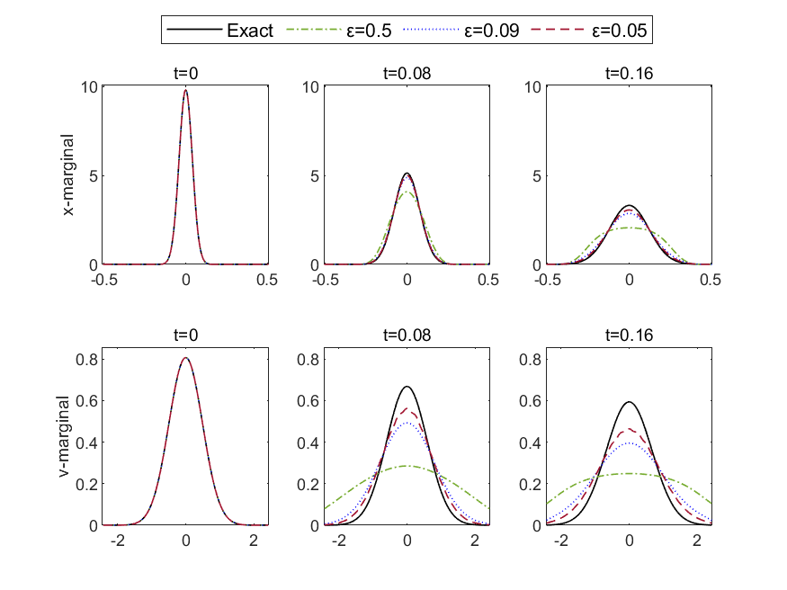
Figure 4.1: Comparison between the exact solution (black line) and our entropy regularised scheme for the position $x$-marginal and velocity $v$-marginal, across three time-slices $t=0,0.08,0.16$ and three regularisation choices $\varepsilon=0.5,0.09,0.05$. Simulation over the position-velocity domain $[-0.5,0.5]\times[-2.5,2.5]$. All cases are ran with a step-size of $h=0.02$.

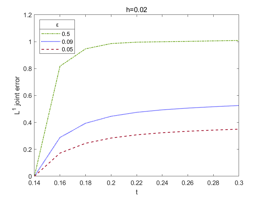
Figure 4.2: $L^{1}(\Lambda)$-norm joint error of the regularised scheme as a map of time over $[0.14,0.3]$ for multiple regularisation parameters $\varepsilon=0.5,0.09,0.05$. Simulation over the position-velocity domain $[-0.5,0.5]\times[-2.5,2.5]$. All cases are ran with a step-size of $h=0.02$.

We now discuss some of the drawbacks of the numerical implementation of this JKO type scheme. As pointed out already, regularisation introduces blurring into the system giving less sharp results. To circumvent this, one takes a small value for the regularisation parameter, however this causes numerical underflow due to the exponential form of the Gibbs Kernel $K$ (defined just above (4.3)). For the vanilla Sinkhorn algorithm this is discussed in [62, Remark 4.7], and for more general scaling algorithms see [26, 66]. This issue can be partly minimised by carrying out the computations in the log-domain [62, Section 4.4]. Critically, the log-domain strategy is very costly due to many additional operations introduced, the algorithm is no longer just a matrix scaling algorithm. This issue is mitigated to a certain extent by the absorbing algorithm [66, Algorithm 2.]. Domain decomposition techniques [12] also seem a feasible strategy to improve these algorithms.

There is a further added difficulty for schemes with a time-step dependent cost function, such as the ones introduced in our manuscript. Namely, for a fixed spatial discretization, as the time-step tends to zero the cost function “blows up”, which stems from a $O(1/h^{2})$-order term appearing in the cost function (3.14). This (in addition to the $1/\varepsilon$ appearing in the Gibbs Kernel $K$ and discussed above) requires careful tuning, otherwise it will lead to numerical underflow. This suggests an operator-splitting scheme as in [1], which consists of a transport (Hamiltonian flow) step and a steepest descent step capturing the conservative-dissipative structure, may be more favourable in simulating Kramers equation, since the cost function appearing in [1] is only of order $O(1/h)$ (instead of the order $1/h^{2}$ appearing in our cost term).

Lastly, we note that in full rigour one should show the convergence of the fully discretised scheme (4.2) to its continuous version as the volume $\lambda$ of each grid tile tends to zero. Such analysis has been done for many Wasserstein-type gradient flows [9, 44, 53, 54], however it is still an open question for the systems we consider here. As in the mentioned papers, we expect that some conditions, such as Courant–Friedrichs–Lewy (CFL) type condition, need to be imposed on the temporal and spatial meshes to guarantee the convergence of the fully discretised schemes. Revealing such conditions for non-gradient systems is nontrivial and we leave this question for future work.

5 Well Posedness of the Regularised JKO scheme

The main result of this section is Proposition 5.1, stating the existence of a unique minimiser to the optimisation problem (1.6). It is natural to achieve well-posedness of the scheme through finiteness, lower semi-continuity, and convexity of the functionals which appear in it. There exist $h_{0},\varepsilon_{0}>0$ depending only on the constants in our Assumptions, such that all the following results hold for $h_{0}>h>0,\varepsilon_{0}>\varepsilon>0$. Note that we are ultimately interested in the case where $h,\varepsilon\to 0$. We now give the main result of this section, the well-posedness of the optimal transport optimisation problem (1.6).

Proposition 5.1.

Take $h,\varepsilon>0$ small enough with $\frac{\varepsilon}{h}\leq 1$ and $\mu\in\mathcal{P}^{r}_{2}(\mathbb{R}^{d})$ with $\mathcal{F}(\mu)<\infty$. Then, there exists a unique $\nu^{*}\in\mathcal{P}^{r}_{2}(\mathbb{R}^{d})$ such that

$$\nu^{*}=\underset{\nu\in\mathcal{P}^{r}_{2}(\mathbb{R}^{d})}{\text{argmin}}\Big{\{}\frac{1}{2h}\mathcal{W}_{c_{h},\varepsilon}(\mu,\nu)+\mathcal{F}(\nu)\Big{\}}.$$

The proof is provided at the end of the section after stating and proving a sequence of auxiliary results.

5.1 Proofs and auxiliary results

From (2.11) in Assumption 2.5 we immediately have the following result.

Lemma 5.2.

For any $h>0$ small enough, and any $\mu$ and $\nu$ in $\mathcal{P}_{2}(\mathbb{R}^{d})$ with $\gamma$ the associated optimal plan in (1.5), it holds that

$$M(\nu)\leq C\Big{(}(c_{h},\gamma)+M(\mu)\Big{)},$$

where the constant $C>0$ is independent of $h,\varepsilon$.

Proof.

Let $\gamma$ be optimal plan in (1.5) with first marginal $\mu$ and second marginal $\nu$. Since for all $x,y\in\mathbb{R}^{d}$ $\|y\|^{2}\leq 2(\|x\|^{2}+\|x-y\|^{2})$, we have

$$M(\nu)=\int_{\mathbb{R}^{2d}}\|y\|^{2}d\gamma(x,y)\leq 2\int_{\mathbb{R}^{2d}}\|x\|^{2}+\|x-y\|^{2}d\gamma(x,y)$$

$$\leq 2\int_{\mathbb{R}^{2d}}\|x\|^{2}+C\big{(}c_{h}(x,y)+h^{2}(\|x\|^{2}+\|y\|^{2})\big{)}d\gamma(x,y),$$ (5.1)

where in (5.1) we have used (2.11). Hence for some $C>0$

$$M(\nu)\leq C\Big{(}(c_{h},\gamma)+(1+h^{2})M(\mu)+h^{2}M(\nu)\Big{)},$$

which implies that for small enough $h$,

$$M(\nu)\leq C\Big{(}(c_{h},\gamma)+M(\mu)\Big{)}.$$

∎

Of course if $\rho^{n}_{h,\varepsilon},\rho^{n-1}_{h,\varepsilon}$ are built from the scheme (1.4) with associated plan $\gamma^{n}_{h,\varepsilon}$, then Lemma 5.2 says that for small enough $h$

$$M(\rho^{n}_{h,\varepsilon})\leq C\Big{(}(c_{h},\gamma^{n}_{h,\varepsilon})+M(\rho^{n-1}_{h,\varepsilon})\Big{)}.$$ (5.2)

Lemma 5.3 (Weak lower semi-continuity of $\gamma\mapsto(c_{h},\gamma)$).

Let $h>0$. Let $\{\gamma_{k}\}_{k\in\mathbb{N}}\subset\mathcal{P}(\mathbb{R}^{2d})$, $\gamma\in\mathcal{P}(\mathbb{R}^{2d})$, with $\gamma_{k}\rightharpoonup\gamma$. Then

$$(c_{h},\gamma)\leq\liminf_{k\to\infty}(c_{h},\gamma_{k}).$$

Proof.

The map $c_{h}:\mathbb{R}^{2d}\to\mathbb{R}$ is continuous and non-negative by Assumption 2.5, hence the result is given by [67, Lemma 4.3]. ∎

Lemma 5.4 (Weak lower semi-continuity of entropy under bounded 2nd moments).

Let $\{\gamma_{k}\}_{k\in\mathbb{N}}\subset\mathcal{P}_{2}(\mathbb{R}^{2d})$, $\gamma\in\mathcal{P}_{2}(\mathbb{R}^{2d})$ with $\gamma_{k}\rightharpoonup\gamma$. Further assume that there exists a $C>0$, such that for all $k\in\mathbb{N},$ $M(\gamma_{k}),M(\gamma)<C$, then

$$H(\gamma)\leq\liminf_{k\to\infty}H(\gamma_{k}).$$

Proof.

This follows immediately by Lemma A.2 taking $u(a)=a\log(a)$. ∎

Lemma 5.5 (Existence of minimising couplings in the optimal transport problem).

Given $\mu,\nu\in\mathcal{P}^{r}_{2}(\mathbb{R}^{d})$ with finite entropy $H(\mu),H(\nu)<\infty$. Then, there exists a $\gamma\in\Pi^{r}(\mu,\nu)$ which attains the infimum in $\mathcal{W}_{c_{h},\varepsilon}(\mu,\nu)$.

Proof.

By [67, Lemma 4.4] $\Pi(\mu,\nu)$ is tight, and hence by Prokhorov’s Theorem it is also relatively compact. Let $\gamma_{k}\in\Pi(\mu,\nu)$, $k\in\mathbb{N}$, be a minimising sequence of $\mathcal{W}_{c_{h},\varepsilon}(\mu,\nu)$.

Now, using that $\Pi(\mu,\nu)$ is relatively compact, we can say (extracting a sub-sequence and relabelling) that $\gamma_{k}\rightharpoonup\gamma\in\Pi(\mu,\nu)$ (since $\Pi(\mu,\nu)$ is weakly closed). Lemmas 5.3, 5.4 proved lower semi-continuity of $\hat{\gamma}\mapsto(c_{h},\hat{\gamma})$, $\hat{\gamma}\mapsto H(\hat{\gamma})$ respectively, which implies the limit, $\gamma$, is a minimiser.

It remains only to show that $\gamma$ has a density. Using (2.12) (and that there exists an admissible plan, e.g., the product measure $\mu\otimes\nu$) we see that $\mathcal{W}_{c_{h},\varepsilon}(\mu,\nu)<\infty$. Since $\mathcal{W}_{c_{h},\varepsilon}(\mu,\nu)<\infty$ and $(c_{h},\gamma)\geq 0$ we deduce that $H(\gamma)<\infty$, hence $\gamma\in\Pi^{r}(\mu,\nu)$. ∎

So far we have shown that there exists an absolutely continuous transport plan with finite entropy that solves the optimal transport problem (1.5) between any two measures in $\mathcal{P}_{2}^{r}(\mathbb{R}^{d})$. Next, we explore some properties of the Kantorovich optimal transport cost functional $\mathcal{W}_{c_{h},\varepsilon}$ defined by (1.5).

Lemma 5.6 (Strict Convexity of $\nu\mapsto\mathcal{W}_{c_{h},\varepsilon}(\mu,\nu)$).

For a fixed $\mu\in\mathcal{P}_{2}^{r}(\mathbb{R}^{d})$,

$$\mathcal{P}_{2}^{r}(\mathbb{R}^{d})\ni\nu\mapsto\mathcal{W}_{c_{h},\varepsilon}(\mu,\nu),$$

is strictly convex.

Proof.

This follows as in [17, Lemma 2.5] by linearity of $\gamma\mapsto(c_{h},\gamma)$ and strict convexity of $H$. ∎

Lemma 5.7 (Lower semi-continuity of $\nu\mapsto\mathcal{W}_{c_{h},\varepsilon}(\mu,\nu)$ restricted to $\mathcal{P}^{r}_{2}(\mathbb{R}^{d})$ and uniform moment bounds).

Let $\{\nu_{k}\}_{k\in\mathbb{N}}\subset\mathcal{P}_{2}^{r}(\mathbb{R}^{d})$, $\mu,\nu\in\mathcal{P}_{2}^{r}(\mathbb{R}^{d})$, with $\nu_{k}\rightharpoonup\nu$. Moreover, assume for all $k\in\mathbb{N}$ the probability measures $\nu_{k},\mu,\nu$ have uniformly bounded entropy and second moments. Then

$$\mathcal{W}_{c_{h},\varepsilon}(\mu,\nu)\leq\liminf_{k\to\infty}\mathcal{W}_{c_{h},\varepsilon}(\mu,\nu_{k}).$$

Proof.

Let $\{\nu_{k}\},\mu,\nu$ be as assumed above, and $\{\gamma_{k}\}$ be the associated optimal plans in $\mathcal{W}_{c_{h},\varepsilon}(\mu,\nu_{k})$. Note $\{\gamma_{k}\}\subset\Pi(\mu,\{\nu_{k}\})$ (see Notation section). Since $\{\nu_{k}\}$ is weakly convergent it is tight, and [67, Lemma 4.4] implies that $\Pi(\mu,\{\nu_{k}\})$ is too, hence extracting (and relabelling) a sub-sequence $\{\gamma_{k}\}$, we know that $\gamma_{k}\rightharpoonup\gamma\in\mathcal{P}(\mathbb{R}^{2d})$. In fact $\gamma\in\Pi(\mu,\nu)$ since weak convergence of $\gamma_{k}$ implies weak convergence of its marginals (and we know $\nu_{k}\rightharpoonup\nu$). Now, the lower semi-continuity established in Lemmas 5.3 and 5.4 implies that

$$\liminf_{k\to\infty}\mathcal{W}_{c_{h},\varepsilon}(\mu,\nu_{k})=\liminf_{k\to\infty}\frac{1}{2h}(c_{h},\gamma_{k})+\varepsilon H(\gamma_{k}) \geq\frac{1}{2h}(c_{h},\gamma)+\varepsilon H(\gamma)$$

$$\geq\mathcal{W}_{c_{h},\varepsilon}(\mu,\nu).$$

∎

Lemma 5.8.

[Lower-semi continuity of $\mathcal{F}$ under uniformly bounded moments] Let $\{\mu_{k}\}_{k\in\mathbb{N}}\subset\mathcal{P}_{2}(\mathbb{R}^{d})$, $\mu\in\mathcal{P}_{2}(\mathbb{R}^{d})$ with $\mu_{k}\rightharpoonup\mu$. Assume $\sup_{k}M(\mu_{k})<\infty$, then

$$\mathcal{F}(\mu)\leq\liminf_{k\to\infty}\mathcal{F}(\mu_{k}).$$ (5.3)

Proof.

The lower semi-continuity of $U$ follows from the uniform bounded moments, Assumption 2.1 and Lemma A.2. The lower semi-continuity of $F$ follows from [6, Theorem 2.38], since $(x,y):\mathbb{R}^{d}\times\mathbb{R}\to\mathbb{R}$, $(x,y)\mapsto f(x)y$ is clearly 1-homogeneous and convex in $y$ for fixed $x$ (as $f$ is non-negative). ∎

We are now in a position to prove the main result of this section.

Proof of proposition 5.1.

Denote $J_{c_{h},\varepsilon}(\mu,\nu):=\frac{1}{2h}\mathcal{W}_{c_{h},\varepsilon}(\mu,\nu)+\mathcal{F}(\nu)$, and $\gamma$ the optimal coupling in $\mathcal{W}_{c_{h},\varepsilon}(\mu,\nu)$. Note that since $f\geq 0$ and by Lemma A.1 we have, for some fixed $C>0$ and $0<\alpha<1$,

$$J_{c_{h},\varepsilon}(\mu,\nu)\geq\frac{1}{2h}\mathcal{W}_{c_{h},\varepsilon}(\mu,\nu)-C(1+M(\nu))^{\alpha}.$$ (5.4)

Furthermore, since the sum of infima is less than the infima of the sum, and by the property of the entropy and marginals $H(\gamma)\geq H(\mu)+H(\nu)$, we have

$$\frac{1}{2h}\mathcal{W}_{c_{h},\varepsilon}(\mu,\nu)\geq \frac{1}{2h}(c_{h},\gamma)+\frac{\varepsilon}{2h}\big{(}H(\mu)+H(\nu)\big{)}.$$

Moreover, using Lemma 5.2 we have, for $h,\varepsilon>0$ small enough

$$\frac{1}{2h}\mathcal{W}_{c_{h},\varepsilon}(\mu,\nu)\geq \frac{1}{2h}(c_{h},\gamma)+M(\mu)-M(\mu)+\frac{\varepsilon}{2h}\big{(}H(\mu)+H(\nu)\big{)}$$

$$\geq C_{1}M(\nu)+C_{\mu,\varepsilon,h}+\frac{\varepsilon}{2h}H(\nu),\qquad$$

with fixed constants $C_{1}>0$, and $C_{\mu,\varepsilon,h}$ depending only on $\mu,\varepsilon,h$. Consequently by Lemma A.1 we arrive at

$$\frac{1}{2h}\mathcal{W}_{c_{h},\varepsilon}(\mu,\nu)\geq C_{1}M(\nu)+{\color[rgb]{0,0,0}C_{\mu,\varepsilon,h}}-\frac{\varepsilon}{2h}C(1+M(\nu))^{\alpha}.$$ (5.5)

Combining (5.5) with (5.4), and choosing $h,\varepsilon$ small enough we get that

$$J_{c_{h},\varepsilon}(\mu,\nu)\geq C_{1}M(\nu)+{\color[rgb]{0,0,0}C_{\mu,\varepsilon,h}}-C_{1}(1+M(\nu))^{\alpha}.$$ (5.6)

Now employing (A.1), as well as the Bernoulli inequality: $(1+s)^{\alpha}\leq 1+\alpha s$ for all $s\geq-1$ and $\alpha\in(0,1)$, one can see that (5.6) implies that the functional $\nu\mapsto J_{c_{h},\varepsilon}(\mu,\nu)$ is bounded from below. Note that there exists a $\nu\in\mathcal{P}_{2}^{r}(\mathbb{R}^{d})$ such that $J_{c_{h},\varepsilon}(\mu,\nu)<\infty$, for example, take $\nu=\mu$ (and the product plan). Let $\{\nu_{k}\}$ be a minimising sequence of $\nu\mapsto J_{c_{h},\varepsilon}(\mu,\nu)$. Note $M(\nu_{k}),H(\nu_{k})$ are uniformly bounded. Since $M(\nu_{k})$ is uniformly bounded, the set $\{\nu_{k}\}$ is tight, hence extracting a subsequence (not relabelled) we obtain $\nu_{k}\rightharpoonup\nu\in\mathcal{P}(\mathbb{R}^{d})$. Moreover, $\nu\in\mathcal{P}_{2}(\mathbb{R}^{d})$ since uniform bounded 2nd moments and weak convergence implies the limit has a bounded 2nd moment. The lower semi-continuity proved in Lemmas 5.7 and 5.8 ensures that the limit $\nu$ is a minimiser. That $\nu\in\mathcal{P}^{r}_{2}(\mathbb{R}^{d})$ follows since lower semi-continuity of $\mathcal{P}_{2}(\mathbb{R}^{d})\ni\nu\mapsto H(\nu)$ (see Lemma A.2) which implies $H(\nu)$ is finite. Finally the uniqueness of $\nu$ follows from the linearity of $F$, convexity of $U$, and that $\mathcal{W}_{c_{h},\varepsilon}$ is strictly convex by Lemma 5.6. ∎

Remark 5.9.

Note that the strict convexity of the regularisation functional allowed us to easily ensure uniqueness of the minimiser in Proposition 5.1.

6 Proof of the Main Result

This section presents the proof of the main result, Theorem 2.13. We first establish discrete Euler-Lagrange equations for the minimisers of the regularised scheme 1.4, then we derive necessary a priori estimates, and finally we prove the convergence (up to a subsequence) of the scheme.

6.1 Discrete Euler-Lagrange Equations

In this section we study the minimisers of the optimisation problem (1.6). This is done by studying the functional $\frac{1}{2h}\mathcal{W}_{c_{h},\varepsilon}\big{(}\mu,\cdot\big{)}+\mathcal{F}(\cdot)$ (for a fixed $\mu\in\mathcal{P}^{r}_{2}(\mathbb{R}^{d})$) at small perturbations around its minimiser. Recall that Proposition 5.1 ensured well-posedness of (1.6) for small enough $h,\varepsilon>0$, and thus the associated Euler-Lagrange equations will also hold for such $h,\varepsilon$ small enough.

When (1.2) is describing a Wasserstein gradient flow its solution can be viewed as the minimiser of a large deviation rate functional [2]. With this perspective one can view the Euler-Lagrange equations, established below in Lemma 6.2, as the discrete analogue of (2.17).

Throughout this section, for a given vector field $\eta\in C^{\infty}_{c}(\mathbb{R}^{d};\mathbb{R}^{d})$ we call $\Phi:\mathbb{R}_{+}\times\mathbb{R}^{d}\to\mathbb{R}^{d}$ the flow through $\eta$ with dynamics

$$\partial_{s}\Phi_{s}=\eta(\Phi_{s}),\leavevmode\nobreak\ \Phi_{0}=\text{id}.$$ (6.1)

The following result is well established (for instance see [17, Proposition 3.5]).

Lemma 6.1.

Let $\nu\in\mathcal{P}_{2}^{r}(\mathbb{R}^{d})$, and $\eta\in C^{\infty}_{c}(\mathbb{R}^{d};\mathbb{R}^{d})$ with flow $\Phi_{s}$ defined in (6.1). The first variation of the free energy $\mathcal{F}$ (associated with (1.6)) at $\nu$ along $\eta$, and denoted by $\delta\mathcal{F}(\nu,\eta)$, is

$$\delta\mathcal{F}(\nu,\eta):=\frac{d}{ds}\mathcal{F}\big{(}(\Phi_{s})_{\#}\nu\big{)}\Big{|}_{s=0}=\int_{\mathbb{R}^{d}}\nu(y)\Big{\langle}\eta(y),\nabla f(y)\Big{\rangle}dy-\int_{\mathbb{R}^{d}}p(\nu(y))\text{div}(\eta(y))dy.$$ (6.2)

Lemma 6.2 (Euler-Lagrange equation).

Let $\mu\in\mathcal{P}_{2}^{r}(\mathbb{R}^{d})$, and $h,\varepsilon$ be small enough. Let $\nu$ be the optimum in (1.6), and let $\gamma$ be the corresponding optimal plan in $\mathcal{W}_{c_{h},\varepsilon}(\mu,\nu)$. Then, for any $\eta\in C_{c}^{\infty}(\mathbb{R}^{d};\mathbb{R}^{d})$ we have

$$0=\frac{1}{2h}\int_{\mathbb{R}^{2d}}\Big{\langle}\eta(y),\nabla_{y}c_{h}(x,y)\Big{\rangle}d\gamma(x,y)-\frac{\varepsilon}{2h}\int_{\mathbb{R}^{d}}\nu(y)\text{div}(\eta(y))dy+\delta\mathcal{F}(\nu,\eta).$$ (6.3)

In particular, by (2.9), we have for any function $\varphi\in C^{\infty}_{c}(\mathbb{R}^{d})$

$$\frac{1}{h}\int_{\mathbb{R}^{2d}}\Big{\langle}(y -x),\nabla\varphi(y)\Big{\rangle}d\gamma(x,y)$$

$$=\int_{\mathbb{R}^{d}}\nu(y)\Big{\langle}b(y),\nabla\varphi(y)\Big{\rangle}dy+\frac{\varepsilon}{2h}\int_{\mathbb{R}^{d}}\nu(y)\text{div}\big{(}(A+B_{h})\nabla\varphi(y)\big{)}dy$$

$$\qquad-\delta\mathcal{F}(\nu,(A+B_{h})\nabla\varphi)+O(h)(1+\|\nabla\varphi\|_{\infty})\Big{(}M(\mu)+M(\nu)+1\Big{)}+O\big{(}\frac{1}{h}\big{)}(c_{h},\gamma)$$ (6.4)

Proof.

Let $\Phi$ be defined as in (6.1). Since $\nu$ is optimal for the minimisation problem (1.6) we have

$$\frac{1}{2h}\mathcal{W}_{c_{h},\varepsilon}(\mu,\nu)+\mathcal{F}(\nu)\leq \frac{1}{2h}\mathcal{W}_{c_{h},\varepsilon}(\mu,(\Phi_{s})_{\#}\nu)+\mathcal{F}((\Phi_{s})_{\#}\nu),$$

which implies,

$$0\leq \limsup_{s\to 0}\frac{1}{2hs}\Big{(}\mathcal{W}_{c_{h},\varepsilon}(\mu,(\Phi_{s})_{\#}\nu)-\mathcal{W}_{c_{h},\varepsilon}(\mu,\nu)\Big{)}+\delta\mathcal{F}(\nu,\eta).$$ (6.5)

Let $\gamma$ be the optimal coupling in (1.6). Then, for $\tilde{\Phi}_{s}:=(\text{id},\Phi_{s})$, we know $(\tilde{\Phi}_{s})_{\#}\gamma\in\Pi^{r}(\mu,(\Phi_{s})_{\#}\nu)$ so we have

$$\limsup_{s\to 0}\frac{1}{2hs}\Big{(}\mathcal{W}_{c_{h},\varepsilon}(\mu,(\Phi_{s})_{\#}\nu) -\mathcal{W}_{c_{h},\varepsilon}(\mu,\nu)\Big{)}$$

$$\leq\limsup_{s\to 0}\frac{1}{2hs}\Big{(}(c_{h},(\tilde{\Phi}_{s})_{\#}\gamma)-(c_{h},\gamma)+\varepsilon\Big{(}H((\tilde{\Phi}_{s})_{\#}\gamma)-H(\gamma)\Big{)}\Big{)}.$$

By Fatou’s Lemma we have

$$\limsup_{s\to 0}\frac{(c_{h},(\tilde{\Phi}_{s})_{\#}\gamma)-(c_{h},\gamma)}{2hs}{\color[rgb]{0,0,0}\leq}\frac{1}{2h}\int_{\mathbb{R}^{2d}}\Big{\langle}\eta(y),\nabla_{y}c_{h}(x,y)\Big{\rangle}d\gamma(x,y),$$

and also

$$\limsup_{s\to 0}\frac{\varepsilon\Big{(}H((\tilde{\Phi}_{s})_{\#}\gamma)-H(\gamma)\Big{)}}{2hs}\leq \limsup_{s\to 0}\frac{-\varepsilon}{2hs}\Big{(}\int_{\mathbb{R}^{d}}\log(|\text{det}D\Phi_{s}(y)|)-\log(|\text{det}D\Phi_{0}(y)|)d\nu(y)\Big{)}$$

$$= -\frac{\varepsilon}{2h}\int_{\mathbb{R}^{2d}}\nu(y)\text{div}\big{(}\eta(y)\big{)}dy.$$

Injecting this result into (6.5) and substituting $\eta$ for $-\eta$ gives the result. ∎

6.2 A priori estimates

In this section we provide a number of a priori estimates which will help to establish the compactness arguments of Section 6.3. Throughout this section the results hold for each fixed $k\in\mathbb{N}$, that is, for each $h_{k},\varepsilon_{k},N_{k}$ of the sequences satisfying (2.16), and the sequence $\{\rho^{n}_{h_{k},\varepsilon_{k}}\}_{n=0}^{N_{k}-1}$ built from the scheme (1.4) with the associated sequence of optimal couplings $\{\gamma^{n}_{h_{k},\varepsilon_{k}}\}_{n=1}^{N_{k}}$. For notational convenience we omit the dependence on $k$ and simply write $h,\varepsilon,N,\{\rho^{n}\}_{n=0}^{N-1},\{\gamma^{n}\}_{n=1}^{N}$.

Lemma 6.3.

For all $n\in\{1,\ldots,N\}$, we have

$$(c_{h},\gamma^{n})\leq Ch^{2}\Big{(}M(\rho^{n-1})+1\Big{)}-\varepsilon H(\rho^{n})+2h\Big{(}\mathcal{F}(\rho^{n-1})-\mathcal{F}(\rho^{n})\Big{)},$$ (6.6)

for $C>0$ a constant depending only on $\rho_{0}$ and the constants in the assumptions.

In the well established JKO procedure [43, Eqs. (42)-(45)] one compares $\frac{1}{2h}W^{2}_{2}(\rho^{n-1},\rho^{n})+\mathcal{F}(\rho^{n})$ against $\frac{1}{2h}W^{2}_{2}(\rho^{n-1},\rho^{n-1})+\mathcal{F}(\rho^{n-1})$. The term $W^{2}_{2}(\rho^{n-1},\rho^{n-1})$ is zero, and hence one would end up with a control of $W_{2}(\rho^{n-1},\rho^{n})$ in terms of the free energy. However, in the present work, since $\mathcal{W}_{c_{h},\varepsilon}$ is not a metric, we need to pick a new distribution to compare the performance of $\rho^{n}$ against. We judiciously choose such a distribution as to make the cost $c_{h}$ of transporting mass free.

Proof.

This proof has two steps. First, is the choice of the distribution $\rho_{\sigma}$ against which to compare $\rho^{n}$. The second part is carrying out the said comparison.

Step 1: the candidate distribution $\rho_{\sigma}$ and its properties. Let $G\in C^{\infty}_{c}(\mathbb{R}^{d})$ be a probability density, such that $M(G)=1$, $H(G)<\infty$. For a scaling parameter $\sigma>0$, to be chosen later, define $G_{\sigma}(\cdot):=\sigma^{-d}G(\frac{\cdot}{\sigma})$. For $\mathcal{T}_{h}$ defined in Assumption 2.8 define

$$\gamma_{\sigma}(x,y):=\rho^{n-1}(x)G_{\sigma}\big{(}y-\mathcal{T}_{h}(x)\big{)},$$

as a joint distribution with first marginal $\rho^{n-1}$, and second marginal

$$\rho_{\sigma}(y):=\int\gamma_{\sigma}(x,y)dx.$$

Then, the change of variables $y=\mathcal{T}_{h}(x)+\sigma z$ and leaving $x$ unchanged, has Jacobian

$$J(x,z):=\begin{pmatrix}D\mathcal{T}_{h}(x)&\sigma\\ 1&0\end{pmatrix},$$ (6.7)

with determinant $\big{|}\text{det}J(x,z)\big{|}=\sigma^{d}$. Where the entries $\sigma,1,0$ are $d\times d$-dimensional matrices of that entry multiplied by the identity matrix. Applying the change of variable and calculating we have

$$(c_{h},\gamma_{\sigma})= \int_{\mathbb{R}^{d}}c_{h}(x,y)\rho^{n-1}(x)G_{\sigma}(y-\mathcal{T}_{h}(x))dxdy$$

$$= \int_{\mathbb{R}^{d}}c_{h}(x,\mathcal{T}_{h}(x)+\sigma z)\rho^{n-1}(x)G(z)dxdz.$$ (6.8)

Hence by Assumption 2.8, it follows

$$(c_{h},\gamma_{\sigma})\leq C\int_{\mathbb{R}^{2d}}\Big{(}\frac{\sigma}{h^{\beta}}\Big{(}\|z\|^{2}+1\Big{)}+h^{2}\Big{(}\|x\|^{2}+1\Big{)}\Big{)}\rho^{n-1}(x)G(z)dxdz$$

$$= C\Big{(}\frac{\sigma}{h^{\beta}}\Big{(}\int_{\mathbb{R}^{d}}\|z\|^{2}G(z)dz+1\Big{)}+h^{2}\Big{(}\int_{\mathbb{R}^{2d}}\|x\|^{2}\rho^{n-1}(x)dx+1\Big{)}\Big{)}$$

$$= C\Big{(}\frac{\sigma}{h^{\beta}}+h^{2}\big{(}M(\rho^{n-1})+1\big{)}\Big{)}.$$ (6.9)

Moreover, a straightforward calculation gives

$$H(\gamma_{\sigma})= H(\rho^{n-1})-d\log\sigma+H(G).$$ (6.10)

Again by Assumption 2.8 and the change of variables above we have the following estimate for the potential energy

$$F(\rho_{\sigma})= \int_{\mathbb{R}^{d}}f(y)\rho_{\sigma}(y)dy$$

$$\leq \int_{\mathbb{R}^{2d}}\Big{(}|f(y)-f(x)|+f(x)\Big{)}\rho^{n-1}(x)G_{\sigma}(y-\mathcal{T}_{h}(x))dxdy$$

$$= \int_{\mathbb{R}^{2d}}\Big{(}|f(\mathcal{T}_{h}(x)+\sigma z)-f(x)|\Big{)}\rho^{n-1}(x)G(z)dxdy+\int_{\mathbb{R}^{2d}}f(x)\rho^{n-1}(x)G(z)dxdz$$

$$\leq C\int_{\mathbb{R}^{2d}}\Big{(}\frac{\sigma}{h^{\beta}}\Big{(}\|z\|^{2}+1\Big{)}+h\Big{(}\|x\|^{2}+1\Big{)}\Big{)}\rho^{n-1}(x)G(z)dxdz+F(\rho^{n-1})$$

$$\leq C\Big{(}\frac{\sigma}{h^{\beta}}+h\Big{(}M(\rho^{n-1})+1\Big{)}\Big{)}+F(\rho^{n-1}).$$ (6.11)

Jensen’s inequality implies (by the convexity of $u$) that for the internal energy

$$U(\rho_{\sigma})=\int_{\mathbb{R}^{d}}u\Big{(}\int_{\mathbb{R}^{d}}\gamma_{\sigma}(x,y)dx\Big{)}dy\leq\int_{\mathbb{R}^{2d}}u(\rho^{n-1})G_{\sigma}(y-\mathcal{T}_{h}(x))dxdy=U(\rho^{n-1}).$$ (6.12)

Therefore, plugging (6.11) and (6.12) together yields

$$\mathcal{F}(\rho_{\sigma}) \leq C\Big{(}\frac{\sigma}{h^{\beta}}+h\Big{(}M(\rho^{n-1})+1\Big{)}\Big{)}+F(\rho^{n-1})+U(\rho^{n-1})$$

$$=C\Big{(}\frac{\sigma}{h^{\beta}}+h\Big{(}M(\rho^{n-1})+1\Big{)}\Big{)}+\mathcal{F}(\rho^{n-1}).$$ (6.13)

Step 2: comparing $\rho_{\sigma}$ and $\rho^{n}$. Since the $\{\rho^{n}\}$ are built from the scheme (1.4), and $\gamma_{\sigma}$ is a coupling of $\rho^{n-1}$ and $\rho_{\sigma}$, we have

$$\frac{1}{2h}\Big{(}(c_{h},\gamma^{n})+\varepsilon H(\gamma^{n})\Big{)}+\mathcal{F}(\rho^{n})\leq\frac{1}{2h}\mathcal{W}_{c_{h},\varepsilon}(\rho^{n-1},\rho_{\sigma})+\mathcal{F}(\rho_{\sigma})\leq\frac{1}{2h}\Big{(}(c_{h},\gamma_{\sigma})+\varepsilon H(\gamma_{\sigma})\Big{)}+\mathcal{F}(\rho_{\sigma}).$$ (6.14)

Substituting the above calculations (6.9), (6.10) and (6.2) into (6.14) we get

$$\frac{1}{2h}\Big{(}(c_{h},\gamma^{n})+\varepsilon H(\gamma^{n})\Big{)}+\mathcal{F}(\rho^{n})\leq \frac{1}{2h}\Big{(}C\Big{(}\frac{\sigma}{h^{\beta}}+h^{2}\Big{(}M(\rho^{n-1})+1\Big{)}\Big{)}+\varepsilon\Big{(}H(\rho^{n-1})-d\log\sigma+H(G)\Big{)}\Big{)}$$

$$+C\Big{(}\frac{\sigma}{h^{\beta}}+h\Big{(}M(\rho^{n-1})+1\Big{)}\Big{)}+\mathcal{F}(\rho^{n-1}).$$ (6.15)

Rearranging the terms and using that $H(\gamma^{n})\geq H(\rho^{n})+H(\rho^{n-1})$ we obtain

$$(c_{h},\gamma^{n})\leq C\Big{(}\frac{\sigma}{h^{\beta}}+h^{2}\Big{(}M(\rho^{n-1})+1\Big{)}\Big{)}+\varepsilon\Big{(}-H(\rho^{n})-d\log\sigma+H(G)\Big{)}$$

$$+2hC\Big{(}\frac{\sigma}{h^{\beta}}+h\Big{(}M(\rho^{n-1})+1\Big{)}\Big{)}+2h\Big{(}\mathcal{F}(\rho^{n-1})-\mathcal{F}(\rho^{n})\Big{)}.$$ (6.16)

Now we are free to choose $\sigma=\varepsilon^{1+\frac{\beta}{2}}$. Recall that the scaling (2.16) implies $\frac{\sigma}{h^{\beta}}\leq Ch^{2}$ and $-\varepsilon d\log\sigma\leq(1+\frac{\beta}{2})\varepsilon d\log|\varepsilon|$, we thus have

$$(c_{h},\gamma^{n})\leq Ch^{2}\Big{(}M(\rho^{n-1})+1\Big{)}-\varepsilon H(\rho^{n})+2h\Big{(}\mathcal{F}(\rho^{n-1})-\mathcal{F}(\rho^{n})\Big{)}.$$

∎

From Lemma 6.3 we are able to establish uniform boundedness of the 2nd moment, energy and entropy, of the solutions to the variational scheme (1.4). This is the result we present next. One should note that in the following bounds the constant $C$ depends on the dimension $d$, the constants of our assumptions, the initial data $\rho^{0}$, but importantly is independent of $k$. We mention that the following proof differs from classical a-priori bounds for a JKO scheme since $c_{h}$ is not assumed to be a metric. We follow a similar strategy to that found in [35, 41], first obtaining bounds locally and then extending them over the full time interval.

Lemma 6.4 (Bounded Moments, Energy, and Entropy).

For small enough $h,\varepsilon>0$, we have for all $n\in\{1,\ldots,N\}$

$$M(\rho^{n}),\mathcal{F}(\rho^{n}),-H(\rho^{n})<C.$$ (6.17)

Proof.

We begin by finding an $h_{0},T_{0}$ independent of the initial data, and a $C_{0}$ depending only on $M(\rho^{0}),\mathcal{F}(\rho^{0})$ such that

$$M(\rho^{n}),\mathcal{F}(\rho^{n}),-H(\rho^{n})<C_{0}.$$ (6.18)

holds for all $n\leq\big{\lceil}\frac{T_{0}}{h}\big{\rceil}$ with $h\leq h_{0}$. Now for any $i\in\{1,\ldots,N\}$

$$M(\rho^{i})^{\frac{1}{2}}\leq M(\rho^{i-1})^{\frac{1}{2}}+W_{2}(\rho^{i-1},\rho^{i})$$ (6.19)

$$\leq M(\rho^{i-1})^{\frac{1}{2}}+C\Big{(}(c_{h},\gamma^{i})+h^{2}(M(\rho^{i-1})+M(\rho^{i})\Big{)}^{\frac{1}{2}}$$ (6.20)

$$\leq M(\rho^{i-1})^{\frac{1}{2}}+C\Big{(}(c_{h},\gamma^{i})^{\frac{1}{2}}+h(M(\rho^{i-1})^{\frac{1}{2}}+M(\rho^{i})^{\frac{1}{2}})\Big{)},$$

where in (6.19) we have used the Minkowski integral inequality, and in (6.20) we have used Lemma 5.2. Summing over $i=1,\ldots,n$, and denoting $M^{0}=M(\rho^{0})$ we get

$$M(\rho^{n})^{\frac{1}{2}}\leq C\Big{(}(M^{0})^{\frac{1}{2}}+\sum_{i=1}^{n}(c_{h},\gamma^{i})^{\frac{1}{2}}+h\sum_{i=1}^{n}M(\rho^{i})^{\frac{1}{2}}\Big{)}.$$ (6.21)

Squaring (6.21), and then using Cauchy–Schwarz inequality we get

$$M(\rho^{n})\leq C\Big{(}M^{0}+\big{(}\sum_{i=1}^{n}(c_{h},\gamma^{i})^{\frac{1}{2}}\big{)}^{2}+h^{2}\big{(}\sum_{i=1}^{n}M(\rho^{i})^{\frac{1}{2}}\big{)}^{2}\Big{)}$$

$$\leq C\Big{(}M^{0}+n\sum_{i=1}^{n}(c_{h},\gamma^{i})+h^{2}n\sum_{i=1}^{n}M(\rho^{i})\Big{)}.$$

Now applying Lemma (6.3), and recalling $Nh=T$, we have

$$M(\rho^{n})\leq C\Big{(}M^{0}-n\varepsilon\sum_{i=1}^{n}H(\rho^{i})+2hn\Big{(}\mathcal{F}(\rho^{0})-\mathcal{F}(\rho^{n})\Big{)}+h\sum_{i=1}^{n}M(\rho^{i})\Big{)},$$

Next recalling that $f$ is positive, and using Lemma A.1 twice, we can deduce

$$M(\rho^{n})\leq C_{1}\Big{(}C_{0}+\varepsilon n\sum_{i=1}^{n}(1+M(\rho^{i}))^{\alpha}+(1+M(\rho^{n}))^{\alpha}+h\sum_{i=1}^{n}M(\rho^{i})\Big{)},$$ (6.22)

for some fixed constant $C_{0}>0$ depending only on $M(\rho^{0}),\mathcal{F}(\rho^{0})$, and a fixed the constant $C_{1}>0$ independent of the initial condition. Fixing a time horizon $T_{0}$ small enough, and $N_{0}:=\big{\lceil}\frac{T_{0}}{h}\big{\rceil}$, we let $h_{0}$ be such that for all $h\leq h_{0}$, $N_{0}h\leq 2T_{0}$. Therefore, for all $h\leq h_{0}$, and any $n_{0}\leq N_{0}$, summing (6.22) over $n=1,\ldots,n_{0}$,

$$\sum_{n=1}^{n_{0}}M(\rho^{n})\leq C_{1}\Big{(}n_{0}C_{0}+(n_{0}^{2}\varepsilon+1)\sum_{n=1}^{n_{0}}(1+M(\rho^{n}))^{\alpha}+hn_{0}\sum_{n=1}^{n_{0}}M(\rho^{n})\Big{)},$$

Choosing $T_{0}$ small enough that $C_{1}hN_{0}\leq\frac{1}{2}$, one can see that

$$\frac{1}{2}\sum_{n=1}^{n_{0}}M(\rho^{n})\leq C_{1}\Big{(}n_{0}C_{0}+(n_{0}^{2}\varepsilon+1)\sum_{n=1}^{n_{0}}(1+M(\rho^{n}))^{\alpha}\Big{)}.$$ (6.23)

Substituting (6.23) into the last term in (6.22) we have, for all $n\leq N_{0}$ and $h\leq h_{0}$,

$$M(\rho^{n})\leq C_{1}\Bigg{(}C_{0}+\varepsilon n\sum_{i=1}^{n}(1+M(\rho^{i}))^{\alpha}+(1+M(\rho^{n}))^{\alpha}+2hC_{1}\Big{(}nC_{0}+(n^{2}\varepsilon+1)\sum_{n=1}^{n}(1+M(\rho^{n}))^{\alpha}\Big{)}\Bigg{)}.$$

Using $nh\leq T$ in conjunction with the scaling (2.16), specifically $\varepsilon\leq Ch^{2}$, the above inequality simplifies to

$$M(\rho^{n})\leq \tilde{C}_{1}\Big{(}\tilde{C}_{0}+h\sum_{i=1}^{n}(1+M(\rho^{i}))^{\alpha}\Big{)},$$ (6.24)

for some new fixed constant $\tilde{C}_{0}>0$ depending only on $M(\rho^{0}),\mathcal{F}(\rho^{0})$, and a fixed the constant $\tilde{C}_{1}>0$ independent of the initial condition. Let $\bar{M}=\max_{n\leq N_{0}}M(\rho^{n})$. Since (6.24) holds for all $n\leq N_{0}$, this implies that

$$\bar{M}\leq \tilde{C}_{1}\Big{(}\tilde{C}_{0}+hN_{0}(1+\bar{M})^{\alpha}\Big{)}.$$ (6.25)

Choose $T_{0}$ small enough that $\tilde{C}_{1}hN_{0}\leq\frac{1}{2}$. From (6.25) we can use the Bernoulli inequality to claim, for some new fixed constant $C_{0}>0$ depending only on $M(\rho^{0}),\mathcal{F}(\rho^{0})$, that for all $h\leq h_{0},n\in\{0,\ldots,N_{0}\}$ with $N_{0}=\lceil\frac{T_{0}}{h}\rceil$

$$M(\rho^{n})\leq C_{0},-H(\rho^{n})\leq C_{0},$$ (6.26)

where we recall that $T_{0},h_{0}$ are all independent of the initial condition. Now we obtain a similar bound for $\mathcal{F}(\rho^{n})$. Returning to Lemma 6.3, and using the non-negativity of $c_{h}$, we see that for any $i\in\{1,\ldots,N\}$

$$h\big{(}\mathcal{F}(\rho^{i})-\mathcal{F}(\rho^{i-1})\big{)}\leq Ch^{2}\big{(}1+M(\rho^{i})\big{)}-\varepsilon H(\rho^{i}).$$ (6.27)

Upon rearranging (6.27), employing (A.1), and using the Bernoulli inequality, we get that

$$\mathcal{F}(\rho^{i})-\mathcal{F}(\rho^{i-1})\leq Ch\big{(}1+M(\rho^{i})\big{)}.$$

Summing the above inequality over $i=1,\ldots,n\leq N_{0}$ yields

$$\mathcal{F}(\rho^{n})\leq Ch\sum_{i=1}^{n}\big{(}1+M(\rho^{i})\big{)}+\mathcal{F}(\rho^{0}).$$

Now we can use (6.26) , and that $hN\leq T$ to obtain

$$\mathcal{F}(\rho^{n})\leq C_{0}$$ (6.28)

for all $n\leq N_{0}$. Since the $T_{0}$ and $h_{0}$ we have chosen are independent of the initial data we can extend the bound (6.28) to all $n\in\{1,\ldots,N\}$ similarly as has been done in [41, Lemma 5.3], see also [35], which completes the proof.

∎

Corollary 6.5 (The total sum of the costs).

Let $h$ be sufficiently small, then we have

$$\sum_{i=1}^{N}(c_{h},\gamma^{n})\leq Ch.$$

Proof.

Summing (6.6) over $n$, using the bounds of Lemma 6.4, and the scaling Assumption 2.10 yields the result. ∎

6.3 The limiting procedure

Let $\{\rho^{n}_{h_{k},\varepsilon_{k}}\}_{n=0}^{N_{k}}$ be the solution of our scheme (1.4) with associated optimal plans $\{\gamma^{n}_{h_{k},\varepsilon_{k}}\}_{n=1}^{N_{k}}$, and interpolation $\rho_{k}$ defined in (2.18). For notational convenience throughout this section we write $\rho^{n}_{h_{k},\varepsilon_{k}}=\rho^{n}_{k}$, $\gamma^{n}_{h_{k},\varepsilon_{k}}=\gamma^{n}_{k}$. As is common in the JKO procedure, the a priori estimates give us enough compactness to pass, at least along a subsequence, to the limit of $\rho_{k}$ to some $\rho$ in $L^{1}((0,T)\times\mathbb{R}^{d})$. We show that $\rho$ is in fact a weak solution of (1.2).

Lemma 6.6.

The sequence of interpolations $\rho_{k}:[0,T]\times\mathbb{R}^{d}\to\mathbb{R}$ constructed from (2.18) satisfy for any $\varphi\in C^{\infty}_{c}(\mathbb{R}^{d})$.

$$\int_{0}^{T}\int_{\mathbb{R}^{d}}\rho_{k}(t,x)\Big{(}\frac{\varphi(t+h_{k},x)-\varphi(t,x)}{h_{k}}\Big{)}dxdt=-\int_{0}^{h_{k}}\int_{\mathbb{R}^{d}}\rho^{0}(x)\frac{\varphi(t,x)}{h_{k}}dxdt+Q_{k}+R_{k}+O(h_{k}),$$ (6.29)

where

$$Q_{k}= \int_{0}^{T}\int_{\mathbb{R}^{d}}\rho_{k}(t,y)\Big{(}\Big{\langle}\nabla f(y),\Big{(}A+B_{h_{k}}\Big{)}\nabla\varphi(t,y)\Big{\rangle}-\Big{\langle}b(y),\nabla\varphi(t,y)\Big{\rangle}-\frac{\varepsilon_{k}}{2h_{k}}\text{div}\Big{(}\Big{(}A+B_{h_{k}}\Big{)}\nabla\varphi(t,y)\Big{)}\Big{)}dydt,$$ (6.30)

$$R_{k}= -\int_{0}^{T}\int_{\mathbb{R}^{d}}p(\rho_{k}(t,y))\text{div}\Big{(}\Big{(}A+B_{h_{k}}\Big{)}\nabla\varphi(t,y)\Big{)}dydt.$$ (6.31)

Proof.

Again, for notational convenience, we write $h_{k}=h,\varepsilon_{k}=\varepsilon,N_{k}=N$ omitting the dependence on $k$ but leave the dependence explicit in $\gamma_{k}$ and $\rho_{k}$. Let $t\in[0,T]$, the Taylor expansion yields

$$\int_{\mathbb{R}^{d}}\Big{(}\rho^{n}_{k}(x)-\rho^{n-1}_{k}(x)\Big{)}\varphi(t,x)dx =\int_{\mathbb{R}^{2d}}\Big{(}\varphi(t,y)-\varphi(t,x)\Big{)}d\gamma^{n}_{k}(x,y)$$

$$=\int_{\mathbb{R}^{2d}}\Big{\langle}y-x,\nabla\varphi(t,y)\Big{\rangle}d\gamma^{n}_{k}(x,y)+\kappa_{n}(t),$$ (6.32)

where the remainder $\kappa_{n}$ is bounded using (2.11) and Lemma 6.4, namely,

$$|\kappa_{n}(t)|\leq\frac{1}{2}\|\nabla^{2}\varphi\|_{\infty}\int_{\mathbb{R}^{2d}}\|x-y\|^{2}d\gamma^{n}_{k}(x,y) \leq C\int_{\mathbb{R}^{2d}}\Big{(}c_{h}(x,y)+h^{2}\Big{(}\|x\|^{2}+\|y\|^{2}\Big{)}\Big{)}d\gamma^{n}_{k}(x,y)$$

$$=C\Big{(}(c_{h},\gamma^{n}_{k})+h^{2}\Big{(}M(\rho_{k}^{n-1})+M(\rho_{k}^{n})\Big{)}\Big{)}$$

$$\leq C\Big{(}(c_{h},\gamma^{n}_{k})+h^{2}\Big{)}.$$ (6.33)

From (6.32) and using (6.4), whose $O(\cdot)$ terms absorb (6.33), we have

$$\int_{\mathbb{R}^{d}}\Big{(}\frac{\rho^{n}_{k}(x)-\rho^{n-1}_{k}(x)}{h}\Big{)}\varphi(t,x)dx= \int_{\mathbb{R}^{2d}}\Big{\langle}b(y),\nabla\varphi(t,y)\Big{\rangle}d\gamma^{n}_{k}(x,y)$$

$$+\int_{\mathbb{R}^{d}}\Big{(}p(\rho^{n}_{k}(y))+\frac{\varepsilon}{2h}\rho^{n}_{k}(y)\Big{)}\text{div}\Big{(}\Big{(}A+B_{h}\Big{)}\nabla\varphi(t,y)\Big{)}dy$$

$$- \int_{\mathbb{R}^{d}}\rho^{n}_{k}(y)\Big{\langle}\nabla f(y),\Big{(}A+B_{h}\Big{)}\nabla\varphi(t,y)\Big{\rangle}dy$$

$$+ O(h)(1+\|\nabla\varphi\|_{\infty})\Big{(}M(\rho_{k}^{n-1})+M(\rho_{k}^{n})+1\Big{)}+O\Big{(}\frac{1}{h}\Big{)}(c_{h},\gamma^{n}_{k}).$$ (6.34)

Integrating over the interval $(t_{n-1},t_{n})$, and summing over $n$ leads to

$$\sum_{n=1}^{N}\int_{t_{n-1}}^{t_{n}}\int_{\mathbb{R}^{d}}\Big{(}\frac{\rho^{n}_{k}(x)-\rho^{n-1}_{k}(x)}{h}\Big{)}\varphi(t,x)dxdt$$

$$=\int_{0}^{T}\int_{\mathbb{R}^{d}}\rho_{k}(t,y)\Big{\langle}b(y),\nabla\varphi(t,y)\Big{\rangle}dydt+\int_{0}^{T}\int_{\mathbb{R}^{d}}\Big{(}p(\rho_{k}(t,y))+\frac{\varepsilon}{2h}\rho_{k}(t,y)\Big{)}\text{div}\Big{(}\Big{(}A+B_{h}\Big{)}\nabla\varphi(t,y)\Big{)}dydt$$

$$\qquad-\int_{0}^{T}\int_{\mathbb{R}^{d}}\rho_{k}(t,y)\Big{\langle}\nabla f(y),\Big{(}A+B_{h}\Big{)}\nabla\varphi(t,y)\Big{\rangle}dydt+O(h),$$ (6.35)

$$=-Q_{k}-R_{k}+O(h),$$

where $Q_{k}$ and $R_{k}$ given are by (6.30) and (6.31). To establish the first equality we used the bounded moments result in Lemma 6.4, Corollary 6.5 on the sum of the costs to control for the very last term in (6.34) after being summed up over $n$, and have used that $Nh=T$. By summation by parts, the LHS is equal

$$\sum_{n=1}^{N_{k}}\int_{t_{n-1}}^{t_{n}}\int_{\mathbb{R}^{d}}\Big{(}\frac{\rho^{n}_{k}(x)-\rho^{n-1}_{k}(x)}{h}\Big{)}\varphi(t,x)dxdt$$

$$\qquad\qquad=-\int_{0}^{h}\int_{\mathbb{R}^{d}}\rho^{0}(x)\frac{\varphi(t,x)}{h}dxdt+\int_{0}^{T}\int_{\mathbb{R}^{d}}\rho_{k}(t,x)\Big{(}\frac{\varphi(t,x)-\varphi(t+h,x)}{h}\Big{)}dxdt.$$ (6.36)

Joining (6.3) and (6.3), and re-arranging gives the result (6.29). ∎

Inline with the classical strategy developed in [43] we are left to take limits in (6.29). The convergence of the additional terms involving $b,\frac{\varepsilon}{h}$ is easy since they are linear in $\rho_{k}$ and we have the scaling (2.16). The convergence of the non-linear term is dealt with in the following Section, after which we conclude the proof of Theorem 2.13.

Strong Convergence of the pressure of $\rho_{k}$

We emphasise the weak convergence of $\rho_{k}$ is not enough to deal with convergence of the non-linear term

$$\int_{0}^{T}\int_{\mathbb{R}^{d}}p(\rho_{k}(t,y))\text{div}\Big{(}\Big{(}A+B_{h}\Big{)}\nabla\varphi(t,y)\Big{)}dydt.$$

Instead, the convergence of $\rho_{k}\to\rho$ in $L^{m}([0,T],\mathbb{R}^{d})$ is obtained via the compactness argument [65, Theorem 2] similar to that done in [17, 18]. Then, (2.6) implies $p$ is continuous from $L^{m}([0,T],\mathbb{R}^{d})$ to $L^{1}([0,T],\mathbb{R}^{d})$ and hence $p(\rho_{k})\to p(\rho)$ in $L^{1}([0,T],\mathbb{R}^{d})$.

Lemma 6.7.

Consider the sequence of interpolations $\rho_{k}:[0,T]\times\mathbb{R}^{d}\to\mathbb{R}$ constructed from (2.18), and $m\in\mathbb{N}$ introduced in Assumption 2.1. For $k$ large enough we have that

$$\int_{0}^{T}\int_{\mathbb{R}^{d}}\big{(}(\rho_{k}(t,y))^{m}+\|\nabla(\rho_{k}(t,y))^{m}\|\big{)}dydt\leq C,$$ (6.37)

where $C>0$ independent of $k$.

Proof.

The estimate of Lemma 6.4 and (2.7) yield directly

$$\int_{0}^{T}\int_{\mathbb{R}^{d}}(\rho_{k}(t,y))^{m}dydt\leq C.$$

It remains to show

$$\int_{0}^{T}\int_{\mathbb{R}^{d}}\|\nabla(\rho_{k}(t,y))^{m}\|dydt\leq C.$$ (6.38)

Omit the dependence on $k$ from $\rho^{n}_{k}=\rho^{n}$ and $\gamma^{n}_{k}=\gamma^{n}$ for this proof. Set $\mu^{n}:=\frac{\varepsilon}{2h}\rho^{n}+p(\rho^{n})$ and notice that $\mu^{n}\in L^{1}(\mathbb{R}^{d})$ by (2.7) and Lemma 6.4. From the Euler-Lagrange equation Lemma 6.2

$$\int_{\mathbb{R}^{d}}\mu^{n}(y)\text{div}(\eta(y))dy=\frac{1}{2h}\int_{\mathbb{R}^{2d}}\Big{\langle}\nabla_{y}c_{h}(x,y),\eta(y)\Big{\rangle}d\gamma^{n}(x,y)+\int_{\mathbb{R}^{d}}\Big{\langle}\rho^{n}(y)\nabla f(y),\eta(y)\Big{\rangle}dy.$$ (6.39)

Since $\gamma^{n}\in\Pi^{r}(\rho^{n-1},\rho^{n})$, by the disintegration of measures Theorem [6, Theorem 2.28] there exists a measure valued map $y\to\gamma^{n}_{y}$ such that $\gamma^{n}=\gamma_{y}^{n}\times\rho^{n}$, so that one can write

$$\int_{\mathbb{R}^{2d}}\Big{\langle}\nabla_{y}c_{h}(x,y),\eta(y)\Big{\rangle}d\gamma^{n}(x,y)=\int_{\mathbb{R}^{d}}\Big{\langle}\eta(y),\Big{(}\rho^{n}(y)\int_{\mathbb{R}^{d}}\nabla_{y}c_{h}(x,y)\gamma_{y}^{n}(x)dx\Big{)}\Big{\rangle}dy.$$

Note that, for each fixed $h>0$, $y\mapsto\big{(}\rho^{n}(y)\int_{\mathbb{R}^{d}}\nabla_{y}c_{h}(x,y)\gamma_{y}^{n}(x)dx\big{)}\in L^{1}(\mathbb{R}^{d})$, since by (2.10) and Lemma 6.4,

$$\int_{\mathbb{R}^{d}}\Big{|}\rho^{n}(y)\int_{\mathbb{R}^{d}}\nabla_{y}c_{h}(x,y)\gamma_{y}^{n}(x)dx\Big{|}dy\leq \int_{\mathbb{R}^{2d}}\|\nabla_{y}c_{h}(x,y)\|\gamma^{n}(x,y)dxdy$$

$$\leq C(h)\Big{(}M(\rho^{n})+M(\rho^{n-1})+1\Big{)}<\infty.$$

Moreover, since $f$ is differentiable and Lipschitz it is clear that $y\mapsto\rho^{n}(y)\nabla f(y)\in L^{1}(\mathbb{R}^{d})$. Hence $\mu^{n}$ has a weak derivative $\nabla\mu^{n}\in L^{1}(\mathbb{R}^{d})$. Moreover, we prove next that $\mu^{n}\in\text{BV}(\mathbb{R}^{d})$, concretely,

$$\Big{|}\int_{\mathbb{R}^{d}}\mu^{n}(y)\text{div}(\eta(y))dy\Big{|}\leq \Big{|}\frac{1}{2h}\int_{\mathbb{R}^{2d}}\Big{\langle}\nabla_{y}c_{h}(x,y),\eta(y)\Big{\rangle}d\gamma^{n}(x,y)dxdy\Big{|}+C\|\eta\|_{\infty}$$ (6.40)

$$= \Big{|}\frac{1}{h}\int_{\mathbb{R}^{2d}}\Big{\langle}\Big{(}(y-x)-hb(y)\Big{)},(A+B_{h})\eta(y)\Big{\rangle}d\gamma^{n}(x,y)\Big{|}$$ (6.41)

$$+\Big{|}O(h)(1+\|\eta\|_{\infty})(M(\rho^{n-1})+M(\rho^{n})+1)+O\Big{(}\frac{1}{h}\Big{)}(c_{h},\gamma^{n})\Big{|}+C\|\eta\|_{\infty},$$

where (6.40) follows using that $f$ is differentiable and Lipschitz, and (6.41) follows by (2.9). Notice now that the moments in (6.41) are finite because of Lemma 6.4 and the $O(h)$ terms are dominated by a constant $C$. Therefore,

$$\eqref{z2}\leq \Big{|}\frac{1}{h}\int_{\mathbb{R}^{2d}}\Big{\langle}\Big{(}(y-x)-hb(y)\Big{)},(A+B_{h})\eta(y)\Big{\rangle}d\gamma^{n}(x,y)\Big{|}$$ (6.42)

$$+O\Big{(}\frac{1}{h}\Big{)}(c_{h},\gamma^{n})+C\Big{(}1+\|\eta\|_{\infty}\Big{)}.$$

Consider the first term in (6.42)

$$\Big{|}\frac{1}{h}\int_{\mathbb{R}^{2d}}\Big{\langle}\Big{(}(y-x)-hb(y)\Big{)},(A+B_{h})\eta(y)\Big{\rangle}d\gamma^{n}(x,y)\Big{|}$$

$$\leq O(1)\|\eta\|_{\infty}\Big{(}\frac{1}{h}\int_{\mathbb{R}^{2d}}\|x-y\|d\gamma^{n}(x,y)+\int_{\mathbb{R}^{d}}\|b(y)\|\rho^{n}(y)dy\Big{)}$$ (6.43)

$$\leq O(1)\|\eta\|_{\infty}\Big{(}\frac{1}{h}\Big{(}\int_{\mathbb{R}^{2d}}\|x-y\|^{2}d\gamma^{n}(x,y)\Big{)}^{1/2}+1+\int_{\mathbb{R}^{d}}\|y\|^{2}\rho^{n}(y)dy\Big{)}$$ (6.44)

$$\leq O(1)\|\eta\|_{\infty}\frac{1}{h}\Big{(}(c_{h},\gamma^{n})+O(h^{2})\Big{)}^{1/2}+C\|\eta\|_{\infty},$$ (6.45)

where: (6.43) is because of Cauchy Schwartz inequality and that $\|(A+B_{h})\eta\|_{\infty}\leq O(1)\|\eta\|_{\infty}$ when $h<1$. (6.44) follows by Jensen’s inequality and Assumption 2.3. (6.45) follows by (2.11) and Lemma 6.4, the constant $C$ depends only on the moment bound and the vector field $b$. We thus have, using the bound (6.45) in conjunction with (6.42),

$$\Big{|}\int_{\mathbb{R}^{d}}\mu^{n}(y)\text{div}(\eta(y))dy\Big{|}\leq \|\eta\|_{\infty}O\Big{(}\frac{1}{h}\Big{)}\Big{(}(c_{h},\gamma^{n})+O(h^{2})\Big{)}^{1/2}$$ (6.46)

$$+O\Big{(}\frac{1}{h}\Big{)}(c_{h},\gamma^{n})+C\Big{(}1+\|\eta\|_{\infty}\Big{)}.$$ (6.47)

Since $\mu^{n}$ has weak derivative $\nabla\mu^{n}\in L^{1}(\mathbb{R}^{d})$ we have that

$$\|\nabla\mu^{n}\|_{L^{1}(\mathbb{R}^{d})}= \sup_{\{\eta\in C^{\infty}_{c}(\mathbb{R}^{d};\mathbb{R}^{d})\leavevmode\nobreak\ :\leavevmode\nobreak\ \sup\|\eta\|\leq 1\}}\int_{\mathbb{R}^{d}}\mu^{n}(y)\text{div}(\eta(y))dy$$ (6.48)

$$\leq C\Big{(}\frac{1}{h}\Big{(}(c_{h},\gamma^{n})+O(h^{2})\Big{)}^{1/2}+\frac{1}{h}(c_{h},\gamma^{n})+1\Big{)},$$ (6.49)

for some $C>0$. Therefore, by Cauchy Schwartz inequality, Corollary 6.5, and the scaling Assumption 2.10, we have

$$h\sum_{n=1}^{N}\|\nabla\mu^{n}\|_{L^{1}(\mathbb{R}^{d})}\leq C\sum_{i=1}^{N}\Big{(}(c_{h},\gamma^{n})+O(h^{2})\Big{)}^{1/2}+\sum_{n=1}^{N}(c_{h},\gamma^{n})+TC$$

$$\leq C\sqrt{N}\Big{(}\sum_{i=1}^{N}(c_{h},\gamma^{n})+O(h^{2})\Big{)}^{1/2}+C\leq C\sqrt{Nh}+C\leq C,$$ (6.50)

for a constant $C$ independent of $k$. To finish the proof we provide a sketch of the argument and refer the reader to [17, Proposition 3.13] for the full details. One can show that $\|(\rho^{n})^{m-1}\nabla\rho^{n}\|\leq C\|\nabla\mu^{n}\|$, so that $(\rho^{n})^{m}\in W^{1,1}(\mathbb{R}^{d})$, with

$$\|\nabla(\rho^{n})^{m}\|\leq C\|\nabla\mu^{n}\|.$$

Therefore, using (6.50)

$$\int_{0}^{T}\int_{\mathbb{R}^{d}}\|\nabla(\rho_{k})^{m}\|dxdt\leq h\sum_{n=1}^{N}\int_{\mathbb{R}^{d}}\|\nabla(\rho^{n})^{m}\|dx\leq Ch\sum_{n=1}^{N}\int_{\mathbb{R}^{d}}\|\nabla(\mu^{n})^{m}\|dx\leq C.$$ (6.51)

∎

By Lemma 6.7 we can use the compactness results in [65, Theorem 2]. That is, following identically [17, Proposition 3.14, Lemma 3.15] we have the following strong convergence (we omit the proof).

Lemma 6.8.

As $k\to\infty$, up to a suitable subsequence if necessary, we have $\rho_{k}\to\rho$ in $L^{m}([0,T],\mathbb{R}^{d})$ and $p(\rho_{k})\to p(\rho)$ in $L^{1}([0,T],\mathbb{R}^{d})$.

6.4 Proof of the main result

We are finally in a position to prove the main result.

Proof of Theorem 2.13.

Taking the limit, up to a subsequence if necessary, $k\to\infty$ ($h,\varepsilon\to 0$, $N\to\infty$) in (6.29) and using the convergence of Lemma 6.8 we can argue the convergence of $Q_{k}$ and $R_{k}$ in (6.29) as follows. For $Q_{k}$ of (6.30) we have

$$\lim_{k\to\infty}Q_{k}=\int_{0}^{T}\int_{\mathbb{R}^{d}}\rho(t,y)\Big{(}\Big{\langle}\nabla f(y),A\nabla\varphi(t,y)\Big{\rangle}-\Big{\langle}b(y),\nabla\varphi(t,y)\Big{\rangle}\Big{)}dydt,$$

since $b$ is continuous (Assumption 2.3), and $\|\nabla f\|$ is uniformly bounded, and we have used the scaling (2.16), namely, ${\varepsilon_{k}}/{h_{k}}\to 0$.

For $R_{k}$ of (6.31) it is clear that

$$\lim_{k\to\infty}R_{k}=-\int_{0}^{T}\int_{\mathbb{R}^{d}}p(\rho(t,y))\text{div}\Big{(}A\nabla\varphi(t,y)\Big{)}dydt$$

We see that the limit $\rho$ satisfies (2.17). ∎

Appendix A Appendix

The following is a well established result that bounds the entropy of a distribution by its second moment.

Lemma A.1.

[43, Proposition 4.1] There exists a $C>0$ and $0<\alpha<1$ such that

$$H(\mu)\geq-C(M(\mu)+1)^{\alpha},\leavevmode\nobreak\ \leavevmode\nobreak\ \forall\mu\in\mathcal{P}_{2}^{r}(\mathbb{R}^{d}).$$ (A.1)

And if $U$ is defined as in Assumption 2.1 then

$$U(\mu)\geq-C(M(\mu)+1)^{\alpha},\leavevmode\nobreak\ \leavevmode\nobreak\ \forall\mu\in\mathcal{P}_{2}^{r}(\mathbb{R}^{d}).$$ (A.2)

Note $C$ is chosen large enough so that (A.1) and (A.2) hold simultaneously.

The next result provides lower semi-continuity for the internal energy and the entropy functional under bounded moments.

Lemma A.2.

[43, Proposition 4.1] Let $u$ satisfy the Assumption 2.1, and $U$ be defined as

$$U(\mu)=\begin{cases}\int_{\mathbb{R}^{d}}u(\mu(x))dx\leavevmode\nobreak\ &\text{if}\leavevmode\nobreak\ \mu\in\mathcal{P}^{r}(\mathbb{R}^{d})\\ \infty\leavevmode\nobreak\ &\text{otherwise}\end{cases}.$$ (A.3)

Then $U$ is weakly lower semi-continuous under bounded moments, i.e if $\{\mu_{k}\}_{k\in\mathbb{N}}\subset\mathcal{P}_{2}(\mathbb{R}^{d})$, $\mu\in\mathcal{P}_{2}(\mathbb{R}^{d})$ with $\mu_{k}\rightharpoonup\mu$, and there exists $C>0$ such that $M(\mu_{k}),M(\mu)<C$ for all $k\in\mathbb{N}$, then

$$U(\mu)\leq\liminf_{k\to\infty}U(\mu_{k}).$$ (A.4)

Appendix B Verification for the examples

B.1 Non-linear diffusion equations

Proof of proposition 3.1.

By Theorem 2.13 one only needs to check that Assumptions 2.1, 2.3, 2.5 and 2.10 hold. The Assumptions 2.1, 2.3 and 2.10 follow directly from the statement of the proposition and hence their verification is omitted.

We now check Assumption 2.5 on the cost function. Clearly (2.10) and (2.12) and (2.13) hold. Let us now verify $\eqref{eq : cost realted to euclidean cost}$. Let $\lambda_{1},\lambda_{2},\ldots$ with $0<\lambda_{1}=h\leq\lambda_{2}\leq\ldots$ be the eigenvalues of $A+hI$. Note for all $i=2,\ldots,d$, $\lambda_{i}=C_{i}+h$ for some $C_{i}\geq 0$. Hence $A+hI$ is invertible, with an inverse $(A+hI)^{-1}$ that is symmetric with eigenvalues $\frac{1}{\lambda_{1}},\frac{1}{\lambda_{2}},\ldots$. Since it is symmetric it is diagonalizable and therefore its normalised eigenvectors form an orthonormal basis. Let $v_{1},\ldots,v_{d}$ be the normalised eigenvectors of $(A+hI)^{-1}$. For any $x\in\mathbb{R}^{d}$ we can write $x=\sum_{i=1}^{d}x_{i}v_{i}$, where $x_{i}:=\langle x,v_{i}\rangle$. Now since $\|x\|^{2}=\sum_{i=1}^{d}x_{i}^{2}$, we have

$$\big{\langle}(A+hI)^{-1}x,x\big{\rangle}= \sum_{i=1}^{d}\frac{1}{{\color[rgb]{0,0,0}\lambda_{i}}}x_{i}^{2}\geq\frac{1}{{\color[rgb]{0,0,0}\lambda_{d}}}\|x\|^{2}\geq\frac{1}{C+2}\|x\|^{2},$$

for $h<1$ and some $C>0$, verifying (2.11). Lastly (2.9) holds by the symmetry of $A+hI$, where we have taken $B_{h}=hI$ in (2.9). To complete the proof it remains only to check the change of variable Assumption 2.8. For this take $\mathcal{T}_{h}(x)=x$, so that (2.14) holds trivially since $c_{h}(x,x+\sigma z)\leq\sigma\|(A+hI)^{-1}\|\|z\|^{2}=\sigma O({h^{-\beta}})\|z\|^{2}$ for some $\beta>0$. Lastly, (2.15) holds with this $\mathcal{T}_{h}$ as $f$ is Lipschitz. ∎

B.2 The non-linear kinetic Fokker-Planck (Kramers) equation

Proof of Proposition 3.3.

By Theorem 2.13 one only needs to check that Assumptions 2.1, 2.3, 2.5, 2.8, and 2.10 hold. The Assumptions 2.1, 2.3, and 2.10 follow directly from the statement of the proposition and hence their verification is omitted. We now check Assumption 2.5 on the cost function. Clearly (2.13) holds. The inequality (2.12) follows by substituting the estimates [35, Eq. (46),(47)] into $c_{h}$, giving $c_{h}(x,v;x^{\prime},v^{\prime})\leq O(h^{-3})(\|x\|^{2}+\|v\|^{2}+\|x^{\prime}\|^{2}+\|v^{\prime}\|^{2})$. The inequality (2.10) is verified by the estimates [35, Eqs. (40a),(40b),(41)] in conjunction with (2.12) just obtained. For (2.11) see [35, Eqs. (39b),(39c)]. For (2.9) we take inspiration from [35], defining, for any $h>0$,

$$B_{h}:=\begin{pmatrix}-\frac{h^{2}}{6}&\frac{h}{2}\\ -\frac{h}{2}&0\end{pmatrix},$$

where, in the matrix $B_{h}$, each entry is a $\tilde{d}\times\tilde{d}$-dimensional matrix of that entry multiplied by the identity matrix. Then for

$$\tilde{\eta}=(A+B_{h})\eta,$$

set $\eta^{1}$ (resp $\eta^{2}$) as the first $\tilde{d}$ components of $\eta$ (resp last $\tilde{d}$ components), and similarly for $\tilde{\eta}$. Then the estimate [35, page 2531]

$$\Big{\langle}\nabla_{x^{\prime}}c_{h}(x,v;x^{\prime},v^{\prime}),\tilde{\eta}^{1} \Big{\rangle}+\Big{\langle}\nabla_{v^{\prime}}c_{h}(x,v;x^{\prime},v^{\prime}),\tilde{\eta}^{2}\Big{\rangle}$$

$$= 2\Big{(}\Big{\langle}x^{\prime}-x,\eta^{1}\Big{\rangle}+\Big{\langle}v^{\prime}-v,\eta^{2}\Big{\rangle}-h\Big{\langle}v^{\prime},\eta^{1}\Big{\rangle}\Big{)}$$

$$+2\Big{\langle}h\nabla g(x^{\prime})+\frac{1}{2}\tau_{h}(x,v;x^{\prime},v^{\prime}),-\frac{h}{2}\eta^{1}+\eta^{2}\Big{\rangle}$$

$$+2\Big{\langle}-h\nabla^{2}g(x^{\prime})v^{\prime}+\frac{1}{2}\sigma_{h}(x,v;x^{\prime},v^{\prime}),-\frac{h^{2}}{6}\eta^{1}+\frac{h}{2}\eta^{2}\Big{\rangle},$$

where [35, Eq. (41)] gives bounds on $\tau_{h},\sigma_{h}$, ensures that (2.9) holds.

We now verify Assumption 2.8 with the change of variables $\mathcal{T}_{h}(x,v)=(x+hv,v)$, consider the admissible, in the sense of (3.12), cubic

$$\bar{\xi}(t)=x+vt+\Big{(}\frac{3}{h^{2}}(x^{\prime}-x-vh)-\frac{v^{\prime}-v}{h}\Big{)}t^{2}+\Big{(}\frac{v^{\prime}+v}{h^{2}}-\frac{2}{h^{3}}(x^{\prime}-x)\Big{)}t^{3},$$

starting at $(x,v)$ and ending at $(x^{\prime},v^{\prime})$. Using Assumption 3.2 we have

$$c_{h}(x,v;x^{\prime},v^{\prime})\leq 2Ch\Big{(}\int_{0}^{h}\|\ddot{\bar{\xi}}(t)\|^{2}dt+\int_{0}^{h}\|\bar{\xi}(t)\|^{2}dt\Big{)}.$$

Note that

$$h\int_{0}^{h}\|\ddot{\bar{\xi}}(t)\|^{2}dt \leq h^{2}\sup_{t\in[0,h}\|\ddot{\bar{\xi}}(t)\|^{2}$$

$$\leq C\Big{(}h^{2}\Big{\|}\frac{3}{h^{2}}\Big{(}x^{\prime}-x-vh\Big{)}-\frac{v^{\prime}-v}{h}\Big{\|}^{2}+h^{4}\Big{\|}\frac{v^{\prime}+v}{h^{2}}-\frac{2}{h^{3}}\Big{(}x^{\prime}-x\Big{)}\Big{\|}^{2}\Big{)},$$

and

$$h\int_{0}^{h}\|\bar{\xi}(t)\|^{2}dt\leq h^{2}\sup_{t\in[0,h]}\|\bar{\xi}(t)\|^{2}$$

$$\leq Ch^{2}\Big{(}\|x\|^{2}+h^{2}\|v\|^{2}+h^{4}\Big{\|}\frac{3}{h^{2}}\Big{(}(x^{\prime}-x-vh\Big{)}-\frac{v^{\prime}-v}{h}\Big{\|}^{2}+h^{6}\Big{\|}\frac{v^{\prime}+v}{h^{2}}-\frac{2}{h^{3}}(x^{\prime}-x)\Big{\|}^{2}\Big{)}.$$

Hence we obtain

$$c_{h}(x,v;x^{\prime},v^{\prime})\leq C\Bigg{(}h^{2}\Big{\|}\frac{3}{h^{2}}\Big{(}x^{\prime}-x-vh\Big{)}-\frac{v^{\prime}-v}{h}\Big{\|}^{2}+h^{4}\Big{\|}\frac{v^{\prime}+v}{h^{2}}-\frac{2}{h^{3}}\Big{(}x^{\prime}-x\Big{)}\Big{\|}^{2}$$

$$+h^{2}\Big{(}\|x\|^{2}+h^{2}\|v\|^{2}+h^{4}\Big{\|}\frac{3}{h^{2}}\Big{(}x^{\prime}-x-vh\Big{)}-\frac{v^{\prime}-v}{h}\Big{\|}^{2}+h^{6}\Big{\|}\frac{v^{\prime}+v}{h^{2}}-\frac{2}{h^{3}}\Big{(}x^{\prime}-x\Big{)}\Big{\|}^{2}\Big{)}\Bigg{)}.$$

So considering $c_{h}(x,v;\mathcal{T}_{h}(x,v)-(\sigma z,\sigma w))$, we have

$$c_{h}(x,v;\mathcal{T}(x,v)-(\sigma z,\sigma w))\leq C\Bigg{(}h^{2}\|\frac{3}{h^{2}}(-\sigma z)-\frac{\sigma w}{h}\|^{2}+h^{4}\|\frac{\sigma w}{h^{2}}-\frac{2}{h^{3}}\sigma z\|^{2}$$

$$+h^{2}\Big{(}\|x\|^{2}+h^{2}\|v\|^{2}+h^{4}\|\frac{3}{h^{2}}(-\sigma z)-\frac{\sigma w}{h}\|^{2}+h^{6}\|\frac{\sigma w}{h^{2}}-\frac{2}{h^{3}}\sigma z\|^{2}\Big{)}\Bigg{)},$$

which proves (2.14). Lastly the Lipschitz property of $f$ gives (2.15), which completes the verification of Assumption 2.8. ∎

Proof of Proposition 3.4.

By Theorem 2.13 one only needs to check that Assumptions 2.1, 2.3, 2.5, 2.8, and 2.10 hold. The Assumptions 2.1, 2.3, and 2.10 follow directly from the statement of the proposition and hence their verification is omitted.

We now check Assumption 2.5 on the cost function. The conditions (2.10), (2.12), (2.13), on $c_{h}$ are easy to verify. For (2.11) see [35, Eqs. (39b),(39c)]. Lastly for (2.9) we again take inspiration from [35] and define for all $h>0$

$$B_{h}:=\begin{pmatrix}-\frac{h^{2}}{6}&\frac{h}{2}\\ -\frac{h}{2}&0\end{pmatrix},$$

where again, in the matrix $B_{h}$, each entry is a $\tilde{d}\times\tilde{d}$-dimensional matrix of that entry multiplied by the identity matrix. One can see from [35, Eq. (60)] does ensure that (2.9) holds.

For Assumption 2.8 take $\mathcal{T}_{h}(x,v)=(x+hv,v)$, we have

$$c_{h}(x,v;\mathcal{T}_{h}(x,v)-(\sigma z,\sigma w))=\|h\nabla g(x)-\sigma z\|^{2}+12\|\frac{1}{2}\sigma w-\frac{1}{h}\sigma z\|^{2}\leq C\Big{(}h^{2}\|x\|^{2}+\|\frac{\sigma}{h}z\|^{2}+\|\sigma w\|^{2}\Big{)},$$

which proves (2.14). Lastly the Lipschitz property of $f$ gives (2.15), which completes the verification of Assumption 2.8. ∎

B.3 A degenerate diffusion equation of Kolmogorov-type

The vector $\mathbf{b}$ and matrix $\mathcal{M}$ which define the cost function (3.21) are of the form

$$\mathbf{b}(h,\mathbf{x},\mathbf{y})=\begin{pmatrix}y_{1}-x_{1}-\frac{h}{1}x_{2}-...-\frac{h^{n-1}}{(n-1)!}x_{n}\\ \vdots\\ h^{i-1}\Big{(}y_{i}-\sum_{j=i}^{n}\frac{h^{j-i}}{(j-i)!}x_{j}\Big{)}\\ \vdots\\ h^{n-1}(y_{n}-x_{n})\end{pmatrix},\qquad\mathcal{M}=\mathcal{M}_{1}\mathcal{M}_{2}^{-1},$$ (B.1)

with $\mathcal{M}_{1},\mathcal{M}_{2}\in\mathbb{R}^{\tilde{d}n\times\tilde{d}n}$ given by

$$(\mathcal{M}_{1})_{ki}=\begin{cases}(-1)^{n-k}\frac{(n+i-1)!}{(k+i-n-1)!},&\quad\text{if}\quad k+i\geq n+1\\ 0&\quad\text{if}\quad k+i<n+1,\end{cases}$$

$$\mathcal{M}_{2}=\left[\begin{array}[]{ccc}1&...&1\\ \begin{pmatrix}n\\ 1\end{pmatrix}&...&\begin{pmatrix}2n-1\\ 1\end{pmatrix}\\ \vdots&\vdots&\vdots\\ k!\begin{pmatrix}n\\ k\end{pmatrix}&...&k!\begin{pmatrix}2n-1\\ k\end{pmatrix}\\ \vdots&\vdots&\vdots\\ (n-1)!\begin{pmatrix}n\\ n-1\end{pmatrix}&...&(n-1)!\begin{pmatrix}2n-1\\ n-1\end{pmatrix}\end{array}\right],$$ (B.8)

where entry of these matrices is to be understood as a $\tilde{d}-$dimensional matrix that is equal to the entry multiplied but the $\tilde{d}-$dimensional identity matrix. The following matrices will also play an important role in the rest of the section

$$J_{1}(h):=\mathrm{diag}(1,h,\cdots,h^{n-1}), D:=\mathrm{diag}(0,\ldots,0,1),$$

$$J_{2}(h):=\begin{pmatrix}1&h&\frac{h^{2}}{2!}&\frac{h^{3}}{3!}&\cdots&\frac{h^{n-1}}{(n-1)!}\\ &h&h^{2}&\frac{h^{3}}{2!}&\cdots&\frac{h^{n-1}}{(n-2)!}\\ &&h^{2}&\frac{h^{3}}{1!}&\cdots&\frac{h^{n-1}}{(n-3)!}\\ &&&\ddots&\cdots&\vdots\\ &&&&&h^{n-1}\end{pmatrix}, Q:=\begin{pmatrix}0\\ 1&0\\ &1&0\\ &&\ddots&\ddots\\ &&&1&0\end{pmatrix}.$$

Omitting the $h$ dependence in $J_{1},J_{2}$ for the sake of clarity, we also define

$$T_{1}:=(2n-1)J_{1}^{T}\mathcal{M}J_{1}-2h(J_{1}^{\prime})^{T}\mathcal{M}J_{1}-h^{2-2n}J_{1}^{T}\mathcal{M}J_{2}DJ_{2}^{T}\mathcal{M}J_{1},$$

$$T_{2}:=(1-2n)J_{2}^{T}\mathcal{M}J_{1}+h\big{(}(J_{2}^{\prime})^{T}\mathcal{M}J_{1}+J_{2}^{T}\,\mathcal{M}\,J_{1}^{\prime}\big{)}-hQJ_{2}^{T}\mathcal{M}J_{1}+J_{2}^{T}\mathcal{M}J_{0}\mathcal{M}J_{1},$$

$$T_{3}:=(2n-1)J_{2}^{T}\mathcal{M}J_{2}-2h(J_{2}^{\prime})^{T}\mathcal{M}J_{2}+2hQJ_{2}^{T}\mathcal{M}J_{2}-h^{2-2n}J_{2}^{T}\mathcal{M}J_{2}DJ_{2}^{T}\mathcal{M}J_{2}.$$

Note that, again, $J_{1},J_{2},Q,D\in\mathbb{R}^{{\tilde{d}n\times\tilde{d}n}}$. Each entry of these matrices should be understood as a matrix of order $\tilde{d}$ that equals the entry multiplied with the $\tilde{d}$-dimensional identity matrix.

We now state a series of results from [37] which will assist us in proving Proposition 3.1.

Lemma B.1 (Proposition 2 of [37]).

The following assertions hold: (1) $T_{1}$ is anti-symmetric, (2) $T_{2}=0$, (3) $T_{3}$ is anti-symmetric, and (4) $\mathrm{Tr}(DJ_{2}^{T}\mathcal{M}J_{2})=n^{2}\tilde{d}h^{2(n-1)}$.

Lemma B.2 (Lemma 4.3 of [37]).

$J_{2}^{-1}J_{1}=J$ where

$$J_{ij}=\begin{cases}0,\quad\text{if}\leavevmode\nobreak\ j<i\\ (-1)^{j-i}\frac{h^{j-i}}{(j-i)!},\quad\text{if}\leavevmode\nobreak\ j\geq i.\end{cases}$$ (B.9)

In particular $J_{ii}=1,\quad J_{ii+1}=-h$ and $J_{ij}=o(h^{2})$ for $j\geq i+2$. Note that $J\in\mathbb{R}^{\tilde{d}n\times\tilde{d}n}$ where $J_{ij}$ should be understood as $J_{ij}I_{\tilde{d}}$.

For any $h>0$ define

$$\mathcal{K}_{h}=h^{2n-2}(J_{2}^{T}\mathcal{M}J_{1})^{-1}.$$ (B.10)

Lemma B.3 (Lemma 4.4 of [37]).

For $\mathcal{K}_{h}$ defined in (B.10) we have

$$(\mathcal{K}_{h})_{ij}=(-1)^{n-j}\frac{h^{2n-i-j}}{(2n-i-j+1)!}.$$ (B.11)

In particular, $(\mathcal{K}_{h})_{nn}=1$ and $(\mathcal{K}_{h})_{ij}=o(h)$ for all $(i,j)\neq(n,n)$. Note also that $\mathcal{K}_{h}\in\mathbb{R}^{\tilde{d}n\times\tilde{d}n}$ where $(\mathcal{K}_{h})_{ij}$ should be understood as $(\mathcal{K}_{h})_{ij}I_{\tilde{d}}$.

With the use of the preceding lemmas we can prove the convergence of the proposed entropic regularised scheme for the degenerate diffusion of Kolmogorov type, Proposition 3.5.

Proof of Proposition 3.5.

By Theorem 2.13 we just need to check Assumptions 2.1, 2.3, 2.5, 2.8, and 2.10 hold.

The scaling Assumption 2.10 and Assumption 2.1 on the internal and potential energy clearly hold. Similarly, its clear that Assumption 2.3 on $b,A$ is also satisfied.

We now show the cost $c_{h}$ defined in (3.21) satisfies Assumption 2.5, with $b,A$ given by (3.15) and $A+B_{h}=\mathcal{K}_{h}$ defined in (B.10). Firstly for (2.11) we take the result directly from [37, Lemma 2.3]. Moreover, one can see that since $\mathcal{M}$ is constant and by definition of $c_{h}$ that (2.12) holds with $C(h)=h^{2-2n}$. From [36, Lemma 2.2] we know that (2.13) holds.

Note we can rewrite $\mathbf{b}$ as

$$\mathbf{b}(h,\mathbf{x},\mathbf{y}) =\begin{pmatrix}y_{1}-x_{1}-\frac{h}{1}x_{2}-...-\frac{{}^{n-1}}{(n-1)!}x_{n}\\ \vdots\\ h^{i-1}\Big{(}y_{i}-\sum_{j=i}^{n}\frac{h^{j-i}}{(j-i)!}x_{j}\Big{)}\\ \vdots\\ h^{n-1}(y_{n}-x_{n})\end{pmatrix}$$

$$=\begin{pmatrix}y_{1}\\ hy_{2}\\ h^{2}y_{3}\\ \vdots\\ h^{n-1}y_{n}\end{pmatrix}-\begin{pmatrix}1&h&\frac{h^{2}}{2!}&\frac{h^{3}}{3!}&\cdots&\frac{h^{n-1}}{(n-1)!}\\ &h&h^{2}&\frac{h^{3}}{2!}&\cdots&\frac{h^{n-1}}{(n-2)!}\\ &&h^{2}&\frac{h^{3}}{1!}&\cdots&\frac{h^{n-1}}{(n-3)!}\\ &&&\ddots&\cdots&\vdots\\ &&&&&h^{n-1}\end{pmatrix}\begin{pmatrix}x_{1}\\ x_{2}\\ x_{3}\\ \vdots\\ x_{n}\end{pmatrix}=J_{1}\mathbf{y}-J_{2}\mathbf{x}.$$

Therefore, we have

$$c_{h}(\mathbf{x},\mathbf{y}) =h^{2-2n}[\mathbf{y}^{T}J_{1}^{T}-\mathbf{x}^{T}J_{2}^{T}]\,\mathcal{M}\,[J_{1}\mathbf{y}-J_{2}\mathbf{x}]$$

$$=h^{2-2n}\Big{[}\mathbf{y}^{T}J_{1}^{T}\,\mathcal{M}\,J_{1}\mathbf{y}-\mathbf{x}^{T}J_{2}^{T}\,\mathcal{M}\,J_{1}\mathbf{y}-\mathbf{y}^{T}J_{1}^{T}\,\mathcal{M}\,J_{2}\mathbf{x}+\mathbf{x}^{T}J_{2}^{T}\mathcal{M}J_{2}\mathbf{x}\Big{]}$$

$$=h^{2-2n}\Big{[}\mathbf{y}^{T}J_{1}^{T}\,\mathcal{M}\,J_{1}\mathbf{y}-2\mathbf{x}^{T}J_{2}^{T}\,\mathcal{M}\,J_{1}\mathbf{y}+\mathbf{x}^{T}J_{2}^{T}\mathcal{M}J_{2}\mathbf{x}\Big{]}.$$

Therefore,

$$\nabla_{\mathbf{y}}c_{h}(\mathbf{x},\mathbf{y})=2h^{2-2n}J_{1}^{T}\mathcal{M}(J_{1}\mathbf{y}-J_{2}\mathbf{x}),$$

so that (2.10) holds with $C(h)=h^{2-2n}$. Hence we are left to prove (2.9). Let $\eta\in\mathbb{R}^{\tilde{d}n}$. We choose $\tilde{\eta}\in\mathbb{R}^{\tilde{d}n}$ such that

$$\begin{pmatrix}\tilde{\eta}_{1}\\ \vdots\\ \tilde{\eta}_{n}\end{pmatrix}=\mathcal{K}_{h}\begin{pmatrix}\eta_{1}\\ \vdots\\ \eta_{n}\end{pmatrix}=\mathcal{K}_{h}\eta,$$

where $\mathcal{K}_{h}$ is given in Lemma B.3, implying that $h^{2-2n}\mathcal{K}_{h}^{T}(J_{1}^{T}MJ_{2})=I$.

Using Lemmas B.2 and B.3, we compute

$$\Big{\langle}\nabla_{\mathbf{y}}c_{h}(\mathbf{x},\mathbf{y}),\tilde{\eta}\Big{\rangle}=\Big{\langle}\nabla_{\mathbf{y}}c_{h}(\mathbf{x},\mathbf{y}),\mathcal{K}_{h}\eta\Big{\rangle} =2\Big{[}(J_{2}^{-1}J_{1}-I)\mathbf{y}\cdot\eta+(\mathbf{y}-\mathbf{x})\cdot\eta\Big{]}$$

$$=2(\mathbf{y}-\mathbf{x})\cdot\eta-2h\sum_{i=2}^{n}y_{i}\cdot\eta_{i-1}+O(h^{2})\|\mathbf{y}\|.$$

For Assumption 2.8, define $\hat{\mathbf{x}}$ as $\hat{\mathbf{x}}_{i}:=\sum_{j=i}^{n}\frac{t^{j-i}}{(j-i)!}\mathbf{x}_{j}$ for $i=1,\dots,n$, and consider the change of variable $\mathcal{T}_{h}(\mathbf{x})=\hat{\mathbf{x}}$. Assumption 2.8 holds with this change of variable and, indeed, one can easily check that

$$c_{h}(\mathbf{x},\mathcal{T}_{h}(\mathbf{x})+\sigma\mathbf{z})\leq Ch^{2-2n}\sigma^{2}\|\mathbf{z}\|^{2},\qquad\textrm{and}\qquad|f(\mathcal{T}_{h}(\mathbf{x})+\sigma\mathbf{z})-f(\mathbf{x})|\leq C\|\sigma z_{n}\|.$$

∎

References

- [1] D. Adams, M. H. Duong, and G. d. Reis. Operator-splitting schemes for degenerate conservative-dissipative systems. arXiv preprint arXiv:2105.11146, 2021.
- [2] S. Adams, N. Dirr, M. Peletier, and J. Zimmer. Large deviations and gradient flows. Philosophical Transactions of the Royal Society A: Mathematical, Physical and Engineering Sciences, 371(2005):20120341, 2013.
- [3] S. Adams, N. Dirr, M. A. Peletier, and J. Zimmer. From a large-deviations principle to the Wasserstein gradient flow: a new micro-macro passage. Comm. Math. Phys., 307(3):791–815, 2011.
- [4] M. Agueh. Existence of solutions to degenerate parabolic equations via the Monge-Kantorovich theory. Adv. Differential Equations, 10(3):309–360, 2005.
- [5] M. Agueh. Local existence of weak solutions to kinetic models of granular media. Archive for Rational Mechanics and Analysis, 221(2):917–959, Aug 2016.
- [6] L. Ambrosio, N. Fusco, and D. Pallara. Functions of bounded variation and free discontinuity problems, volume 254. Clarendon Press Oxford, 2000.
- [7] L. Ambrosio and W. Gangbo. Hamiltonian odes in the wasserstein space of probability measures. Communications on Pure and Applied Mathematics, 61(1):18–53, 2008.
- [8] L. Ambrosio, N. Gigli, and G. Savaré. Gradient flows: in metric spaces and in the space of probability measures. Springer Science & Business Media, 2008.
- [9] R. Bailo, J. A. Carrillo, H. Murakawa, and M. Schmidtchen. Convergence of a fully discrete and energy-dissipating finite-volume scheme for aggregation-diffusion equations. Mathematical Models and Methods in Applied Sciences, 30(13):2487–2522, 2020.
- [10] V. Balakrishnan. Elements of nonequilibrium statistical mechanics, volume 3. Springer, 2008.
- [11] T. Bodineau and R. Lefevere. Large deviations of lattice Hamiltonian dynamics coupled to stochastic thermostats. J. Stat. Phys., 133(1):1–27, 2008.
- [12] M. Bonafini and B. Schmitzer. Domain decomposition for entropy regularized optimal transport. Numerische Mathematik, pages 1–52, 2021.
- [13] M. Burger, M. Franek, and C.-B. Schönlieb. Regularized regression and density estimation based on optimal transport. Applied Mathematics Research eXpress, 2012(2):209–253, 2012.
- [14] K. Caluya and A. Halder. Wasserstein proximal algorithms for the Schrödinger bridge problem: Density control with nonlinear drift. IEEE Transactions on Automatic Control, pages 1–1, 2021.
- [15] K. F. Caluya and A. Halder. Gradient flow algorithms for density propagation in stochastic systems. IEEE Transactions on Automatic Control, 65(10):3991–4004, 2019.
- [16] E. A. Carlen and W. Gangbo. Solution of a model Boltzmann equation via steepest descent in the 2-Wasserstein metric. Arch. Ration. Mech. Anal., 172(1):21–64, 2004.
- [17] G. Carlier, V. Duval, G. Peyré, and B. Schmitzer. Convergence of entropic schemes for optimal transport and gradient flows. SIAM Journal on Mathematical Analysis, 49(2):1385–1418, 2017.
- [18] G. Carlier and M. Laborde. A splitting method for nonlinear diffusions with nonlocal, nonpotential drifts. Nonlinear Analysis: Theory, Methods & Applications, 150:1–18, 2017.
- [19] J. A. Carrillo, K. Craig, and F. S. Patacchini. A blob method for diffusion. Calculus of Variations and Partial Differential Equations, 58(2):1–53, 2019.
- [20] J. A. Carrillo, R. J. McCann, and C. Villani. Kinetic equilibration rates for granular media and related equations: entropy dissipation and mass transportation estimates. Revista Matematica Iberoamericana, 19(3):971–1018, 2003.
- [21] J. A. Carrillo, R. J. McCann, and C. Villani. Contractions in the 2-Wasserstein length space and thermalization of granular media. Arch. Ration. Mech. Anal., 179(2):217–263, 2006.
- [22] J. A. Carrillo and J. S. Moll. Numerical simulation of diffusive and aggregation phenomena in nonlinear continuity equations by evolving diffeomorphisms. SIAM Journal on Scientific Computing, 31(6):4305–4329, 2010.
- [23] P.-H. Chavanis. Generalized thermodynamics and Fokker-Planck equations: Applications to stellar dynamics and two-dimensional turbulence. Phys. Rev. E, 68:036108, Sep 2003.
- [24] P.-H. Chavanis. Nonlinear mean-field Fokker–Planck equations and their applications in physics, astrophysics and biology. Comptes Rendus Physique, 7(3-4):318–330, 2006.
- [25] P.-H. Chavanis, P. Laurençot, and M. Lemou. Chapman-Enskog derivation of the generalized Smoluchowski equation. Phys. A, 341(1-4):145–164, 2004.
- [26] L. Chizat, G. Peyré, B. Schmitzer, and F.-X. Vialard. Scaling algorithms for unbalanced optimal transport problems. Mathematics of Computation, 87(314):2563–2609, 2018.
- [27] S.-N. Chow, W. Huang, Y. Li, and H. Zhou. Fokker-Planck equations for a free energy functional or Markov process on a graph. Arch. Ration. Mech. Anal., 203(3):969–1008, 2012.
- [28] M. Cuturi. Sinkhorn distances: Lightspeed computation of optimal transport. Advances in neural information processing systems, 26:2292–2300, 2013.
- [29] F. Delarue and S. Menozzi. Density estimates for a random noise propagating through a chain of differential equations. Journal of functional analysis, 259(6):1577–1630, 2010.
- [30] S. Di Marino and L. Chizat. A tumor growth model of Hele-Shaw type as a gradient flow. ESAIM Control Optim. Calc. Var., 26:Paper No. 103, 38, 2020.
- [31] M. H. Duong, V. Laschos, and M. Renger. Wasserstein gradient flows from large deviations of many-particle limits. ESAIM: Control, Optimisation and Calculus of Variations, 19(4):1166–1188, 2013.
- [32] M. H. Duong and Y. Lu. An operator splitting scheme for the fractional kinetic Fokker-Planck equation. Discrete Contin. Dyn. Syst., 39(10):5707–5727, 2019.
- [33] M. H. Duong and M. Ottobre. Non-reversible processes: Generic, hypocoercivity and fluctuations, 2021.
- [34] M. H. Duong, M. A. Peletier, and J. Zimmer. GENERIC formalism of a Vlasov-Fokker-Planck equation and connection to large-deviation principles. Nonlinearity, 26(11):2951–2971, 2013.
- [35] M. H. Duong, M. A. Peletier, and J. Zimmer. Conservative-dissipative approximation schemes for a generalized Kramers equation. Math. Methods Appl. Sci., 37(16):2517–2540, 2014.
- [36] M. H. Duong and H. M. Tran. Analysis of the mean squared derivative cost function. Mathematical Methods in the Applied Sciences, 40(14):5222–5240, 2017.
- [37] M. H. Duong and H. M. Tran. On the fundamental solution and a variational formulation for a degenerate diffusion of Kolmogorov type. Discrete Contin. Dyn. Syst., 38(7):3407–3438, 2018.
- [38] M. Erbar, J. Maas, and D. R. M. Renger. From large deviations to Wasserstein gradient flows in multiple dimensions. Electron. Commun. Probab., 20:no. 89, 12, 2015.
- [39] A. Figalli, W. Gangbo, and T. Yolcu. A variational method for a class of parabolic PDEs. Ann. Sc. Norm. Super. Pisa Cl. Sci. (5), 10(1):207–252, 2011.
- [40] U. Gianazza, G. Savaré, and G. Toscani. The Wasserstein gradient flow of the Fisher information and the quantum drift-diffusion equation. Arch. Ration. Mech. Anal., 194(1):133–220, 2009.
- [41] C. Huang. A variational principle for the Kramers equation with unbounded external forces. J. Math. Anal. Appl., 250(1):333–367, 2000.
- [42] C. Huang and R. Jordan. Variational formulations for Vlasov-Poisson-Fokker-Planck systems. Math. Methods Appl. Sci., 23(9):803–843, 2000.
- [43] R. Jordan, D. Kinderlehrer, and F. Otto. The variational formulation of the Fokker-Planck equation. SIAM J. Math. Anal., 29(1):1–17, 1998.
- [44] O. Junge, D. Matthes, and H. Osberger. A fully discrete variational scheme for solving nonlinear fokker–planck equations in multiple space dimensions. SIAM Journal on Numerical Analysis, 55(1):419–443, 2017.
- [45] D. Kinderlehrer and A. Tudorascu. Transport via mass transportation. Discrete and Continuous Dynamical Systems - B, 6(2):311–338, 2006.
- [46] P. Knopp and R. Sinkhorn. Concerning nonnegative matrices and doubly stochastic matrices. Pacific Journal of Mathematics, 21(2):343 – 348, 1967.
- [47] R. C. Kraaij, A. Lazarescu, C. Maes, and M. Peletier. Fluctuation symmetry leads to generic equations with non-quadratic dissipation. Stochastic Processes and their Applications, 130(1):139–170, 2020.
- [48] H. A. Kramers. Brownian motion in a field of force and the diffusion model of chemical reactions. Physica, 7:284–304, 1940.
- [49] S. Lisini. Nonlinear diffusion equations with variable coefficients as gradient flows in Wasserstein spaces. ESAIM Control Optim. Calc. Var., 15(3):712–740, 2009.
- [50] J. Maas. Gradient flows of the entropy for finite Markov chains. J. Funct. Anal., 261(8):2250–2292, 2011.
- [51] A. Marcos and A. Soglo. Solutions of a class of degenerate kinetic equations using steepest descent in Wasserstein space. J. Math., pages Art. ID 7489532, 30, 2020.
- [52] D. Matthes, R. J. McCann, and G. Savaré. A family of nonlinear fourth order equations of gradient flow type. Communications in Partial Differential Equations, 34(11):1352–1397, 2009.
- [53] D. Matthes and H. Osberger. Convergence of a variational lagrangian scheme for a nonlinear drift diffusion equation. ESAIM: M2AN, 48(3):697–726, 2014.
- [54] D. Matthes and B. Söllner. Discretization of flux-limited gradient flows: -convergence and numerical schemes. Mathematics of Computation, 89(323):1027–1057, 2020.
- [55] A. Mielke. Geodesic convexity of the relative entropy in reversible Markov chains. Calc. Var. Partial Differential Equations, 48(1-2):1–31, 2013.
- [56] A. Mielke, M. A. Peletier, and D. R. M. Renger. On the relation between gradient flows and the large-deviation principle, with applications to Markov chains and diffusion. Potential Anal., 41(4):1293–1327, 2014.
- [57] H. C. Öttinger. Beyond equilibrium thermodynamics. Wiley-Interscience, 1st edition, 2005.
- [58] F. Otto. The geometry of dissipative evolution equations: the porous medium equation. Comm. Partial Differential Equations, 26(1-2):101–174, 2001.
- [59] M. Ottobre and G. A. Pavliotis. Asymptotic analysis for the generalized Langevin equation. Nonlinearity, 24(5):1629–1653, 2011.
- [60] M. A. Peletier, R. Rossi, G. Savaré, and O. Tse. Jump processes as generalized gradient flows. Calculus of Variations and Partial Differential Equations, 61(1):33, 2022.
- [61] G. Peyré. Entropic approximation of Wasserstein gradient flows. SIAM J. Imaging Sci., 8(4):2323–2351, 2015.
- [62] G. Peyré, M. Cuturi, et al. Computational optimal transport: With applications to data science. Foundations and Trends® in Machine Learning, 11(5-6):355–607, 2019.
- [63] H. Risken. The Fokker-Planck equation, volume 18 of Springer Series in Synergetics. Springer-Verlag, Berlin, 1984. Methods of solution and applications.
- [64] H. Risken. The Fokker-Planck equation, 1989. Methods of solution and applications.
- [65] R. Rossi and G. Savaré. Tightness, integral equicontinuity and compactness for evolution problems in banach spaces. Annali della Scuola Normale Superiore di Pisa-Classe di Scienze, 2(2):395–431, 2003.
- [66] B. Schmitzer. Stabilized sparse scaling algorithms for entropy regularized transport problems. SIAM Journal on Scientific Computing, 41(3):A1443–A1481, 2019.
- [67] C. Villani. Optimal transport: old and new, volume 338. Springer Science & Business Media, 2008.
- [68] X. Zhang. Variational approximation for Fokker-Planck equation on Riemannian manifold. Probab. Theory Related Fields, 137(3-4):519–539, 2007.