Weak Liouville quantum gravity metrics with matter central charge $\operatorname{\mathbf{c}}\in(-\infty,25)$

Abstract

Physics considerations suggest that a theory of Liouville quantum gravity (LQG) should exist for all values of matter central charge $\mathbf{c}\in(-\infty,25)$. Probabilists have rigorously defined LQG as a random metric measure space for $\mathbf{c}<1$; however, they have only very recently begun to explore LQG in the $\mathbf{c}\in(1,25)$ phase. We define a random metric associated to LQG for all $\mathbf{c}<25$ by a collection of axioms analogous to axioms stated in the $\mathbf{c}<1$ setting. We show that such a metric exists for each $\mathbf{c}$ by considering an approximating metric known as Liouville first passage percolation. Ding and Gwynne proved that these approximating metrics are tight in a suitably chosen topology; we show that every subsequential limit satisfies our axioms. In particular, our result defines a metric associated to LQG in the critical case $\mathbf{c}=1$.

The metrics we define for $\mathbf{c}\in(1,25)$ exhibit geometric behavior that sharply contrasts with the $\mathbf{c}<1$ regime. We show that, for $\mathbf{c}\in(1,25)$, the metrics do not induce the Euclidean topology since they a.s. have a dense (measure zero) set of singular points, points at infinite distance from all other points. We use this fact to prove that a.s. the metric ball is not compact and its boundary has infinite Hausdorff dimension. Despite these differences, we demonstrate that many properties of LQG metrics for $\mathbf{c}<1$ extend in some form to the entire range $(-\infty,25)$. We show that the metrics are a.s. reverse Hölder continuous with respect to the Euclidean metric, are a.s. complete and geodesic away from the set of singular points, and satisfy the bounds for set-to-set distances that hold in the $\mathbf{c}<1$ phase. Finally, we prove that the metrics satisfy a version of the (geometric) Knizhnik-Polyakov-Zamolodchikov (KPZ) formula.

1 Introduction

This paper studies a universal family of random fractal surfaces called Liouville quantum gravity (LQG). The theory of LQG is a subject of active study in the probability community for its applications to conformal field theory, string theory, and other areas of mathematical physics, as well as for its links to the geometry of many classes of random planar maps. LQG was first described heuristically by Polyakov and other physicists in the 1980s; the following is an early formulation of LQG.

Definition 1.1 (Heuristic formulation of LQG).

An LQG surface with matter central charge $\operatorname{\mathbf{c}}\in(-\infty,1]$ and a specified topology (such as the sphere, disk, or torus) is a random surface whose law is given by “the uniform measure on the space of surfaces with this topology” weighted by the $(-\operatorname{\mathbf{c}}/2)$-th power of the determinant of the Laplace-Beltrami operator of the surface.

In this work, we restrict to LQG with simply connected topology; see [DRV16, Rem18, GRV19] for discussion of LQG surfaces that are not simply connected.

The physicists who introduced the theory of LQG believed that a notion of LQG should exist for all real values of $\operatorname{\mathbf{c}}$, and in studying LQG, they were particularly motivated by the regime $\operatorname{\mathbf{c}}\in(1,25)$. Yet, their formulations of LQG do not extend to values of $\operatorname{\mathbf{c}}$ greater than $1$. Physicists have observed [Cat88, Dav97, ADJT93, CKR92, BH92, DFJ84, BJ92, ADF86] through numerical simulations and heuristics that, when $\operatorname{\mathbf{c}}\in(1,25)$, Definition 1.1 describes the geometry of a branched polymer. In mathematical terms, if we model the geometry of Definition 1.1 by a random planar map with a fixed large number $n$ of edges, sampled with probability proportional to the $(-\operatorname{\mathbf{c}}/2)$-th power of the determinant of its discrete Laplacian, we expect that this random planar map model converges as $n\rightarrow\infty$ to an object similar to the continuum random tree (CRT) defined by [Ald91a, Ald91b, Ald93]. This geometry does not depend on $\operatorname{\mathbf{c}}$ and is degenerate from a conformal field theory perspective since it is a tree and not a surface. Physicists have tried to associate a nontrivial geometry to LQG for $\operatorname{\mathbf{c}}\in(1,25)$ despite these apparent obstacles, but have not been successful. See [Amb94] for a survey of these works.

In this paper, we study LQG for $\operatorname{\mathbf{c}}\in(1,25)$ from a rigorous perspective. In recent years, probabilists have translated the heuristic of Definition 1.1 into a rigorous theory of LQG for $\operatorname{\mathbf{c}}\in(-\infty,1)$, constructing both an LQG random measure and an LQG random metric. Their constructions are based on the DDK ansatz of David [Dav88] and Distler-Kawai [DK89], which heuristically describes an LQG surface as a random two-dimensional Riemannian manifold whose Riemannian metric tensor is obtained by exponentiating a multiple of a random distribution $h$ called the Gaussian free field (GFF). (See [She07], [Ber17], [WP20] for a detailed introduction to the GFF.) The LQG measure is constructed by exponentiating a regularized version of $\gamma h$, where $\gamma=\gamma(\operatorname{\mathbf{c}})$ is the coupling constant (see Figure 1). When $\operatorname{\mathbf{c}}\in(1,25)$, this parameter $\gamma$ is complex, which suggests that the LQG random measure does not extend to a real measure for $\operatorname{\mathbf{c}}\in(1,25)$. In contrast, the definition of the LQG metric suggests that it could possibly be defined for $\operatorname{\mathbf{c}}\in(-\infty,25)$. The definition of the metric for $\operatorname{\mathbf{c}}<1$ involves the background charge $Q$ (see Figure 1), which is real and nonzero for $\operatorname{\mathbf{c}}\in(-\infty,25)$.

The idea of defining a metric associated to LQG for $\operatorname{\mathbf{c}}\in(1,25)$ was first explored in [GHPR20], which constructs a heuristic model for such a metric by considering a natural discretization of LQG in terms of dyadic squares that makes sense for all $\operatorname{\mathbf{c}}<25$. This paper, building on the previous work [DG20], rigorously proves the existence of a metric that satisfies a collection of axioms that an LQG metric for $\operatorname{\mathbf{c}}\in(-\infty,25)$ should satisfy. We then apply these axioms to illustrate the key distinguishing features of LQG in this regime and provide a framework for proving results about LQG for $\operatorname{\mathbf{c}}\in(-\infty,25)$. In analogy with the $\operatorname{\mathbf{c}}<1$ setting, we expect—though do not prove—that the axioms we state in this paper uniquely characterize a metric associated to LQG for $\operatorname{\mathbf{c}}\in(-\infty,25)$.

Figure 1: Table of relationships between the values of the matter central charge $\operatorname{\mathbf{c}}$, the background charge $Q$, and the coupling constant $\gamma$. When $\operatorname{\mathbf{c}}\leq 1$, all three parameters are real. When $\operatorname{\mathbf{c}}\in(1,25)$, $\gamma$ is complex, but $Q$ is real and nonzero.

Before stating our results, we review the construction of the LQG random metric in the classical regime $\operatorname{\mathbf{c}}<1$. The DDK ansatz suggests constructing a random metric associated to LQG as a limit of regularized versions of the heuristic metric

$$(z,w)\mapsto\inf_{P:z\rightarrow w}\int_{0}^{1}e^{\xi h(P(t))}|P^{\prime}(t)|\,dt$$

for some $\xi=\xi(\operatorname{\mathbf{c}})$, where the infimum is over all paths from $z$ to $w$. To make this idea precise, we first mollify the field $h$ by the heat kernel; i.e., we set

$$h_{\varepsilon}^{*}(z):=(h*p_{\varepsilon^{2}/2})(z)=\int_{U}h(w)p_{\varepsilon^{2}/2}^{U}(z,w)\,dw,\quad\forall z\in U,$$ (1.1)

where $p_{s}(z,w)=\frac{1}{2\pi s}\exp\mathopen{}\mathclose{{}\left(-\frac{|z-w|^{2}}{2s}}\right)$ is the heat kernel on $\mathbbm{C}$ and the integral (1.1) is interpreted in the sense of distributional pairing. We then define the following regularized metric associated to LQG.

Definition 1.2.

Let $\xi>0$. We define the $\varepsilon$-Liouville first passage percolation (LFPP) metric with parameter $\xi$ associated to the field $h$ as

$$D_{h}^{\varepsilon}(z,w):=\inf_{P:z\rightarrow w}\int_{0}^{1}e^{\xi h_{\varepsilon}^{*}(P(t))}|P^{\prime}(t)|\,dt$$ (1.2)

where the infimum is over all piecewise continuously differentiable paths from $z$ to $w$. We define the rescaled $\varepsilon$-LFPP metric as

$$\mathfrak{a}_{\varepsilon}^{-1}D_{h}^{\varepsilon},$$ (1.3)

where $\mathfrak{a}_{\varepsilon}$ denote the median of the $D_{h}^{\varepsilon}$-distance between the left and right boundaries of the unit square along paths which stay in the unit square.

It is shown in [DG18, Theorem 1.5] and [DG20, Proposition 1.1] that, for every $\xi>0$, there exists $Q=Q(\xi)>0$ with

$$\mathfrak{a}_{\varepsilon}=\varepsilon^{1-\xi Q+o_{\varepsilon}(1)}\qquad\text{as $\varepsilon\rightarrow 0$}$$ (1.4)

Furthermore, $\xi\rightarrow Q(\xi)$ is continuous and nonincreasing on $(0,\infty)$, and tends to $0$ as $\xi\rightarrow\infty$. With $\operatorname{\xi_{\text{crit}}}$ chosen so that $Q(\operatorname{\xi_{\text{crit}}})=2$, we call LFPP for $\xi\in(0,\operatorname{\xi_{\text{crit}}})$ the subcritical phase and LFPP for $\xi\in(\operatorname{\xi_{\text{crit}}},\infty)$ the supercritical phase. Equivalently, if we associate LFPP with parameter $\xi$ to the value of matter central charge associated to background charge $Q(\xi)$ (see Table 1), then the subcritical phase of LFPP corresponds to $\operatorname{\mathbf{c}}<1$, and the supercritical phase of LFPP corresponds to $\operatorname{\mathbf{c}}\in(1,25)$.

Probabilists used the LFPP approximation scheme in the subcritical phase to prove the existence and uniqueness of a random metric associated to LQG for $\operatorname{\mathbf{c}}<1$. They proved this in three stages:

• Stage 1: constructing a candidate metric associated to LQG. First, [DDDF19] constructed a candidate metric associated to LQG for $\operatorname{\mathbf{c}}<1$ by showing that, in the subcritical phase, the laws of the rescaled $\varepsilon$-LFPP metrics are tight in the local uniform topology.

• Stage 2: Showing that this candidate metric satisfies a collection of axioms that characterize the LQG metric. Next, [DFG⁺20] showed that every weak subsequential limit of rescaled $\varepsilon$-LFPP metrics in the subcritical phase can indeed be viewed as a random metric that describes an LQG surface. Specifically, [DFG⁺20] proved that, for each fixed $\xi\in(0,\operatorname{\xi_{\text{crit}}})$, if $\operatorname{\mathbf{c}}\in(-\infty,1)$ is chosen so that $\xi=\xi(\operatorname{\mathbf{c}})$, every subsequential limit of rescaled $\varepsilon$-LFPP metrics satisfies a collection of axioms that a $\operatorname{\mathbf{c}}$-LQG metric should satisfy. These axioms also provide a framework for proving important results about these metrics, such as Hölder continuity and estimates for distances. By applying these estimates, [GP19] showed that, for every metric $D_{h}$ satisfying these axioms, and every set $X\subset\mathbbm{C}$ independent of the field $h$, the Hausdorff dimensions of $X$ with respect to the Euclidean metric and the metric $D_{h}$ are related by the famous KPZ formula (1.12). (We define Hausdorff dimension in Definition 4.1.) Also, the Hausdorff dimension of a metric satisfying the axioms in [DFG⁺20] is equal to the ratio $\xi/\gamma$.

• Stage 3: Proving that the axioms formulated in the previous stage uniquely determine the LQG metric. Finally, the work [GM21] subsequently showed that the axioms stated in [DFG⁺20] characterize a unique metric (up to global rescalings). A key input in this uniqueness proof is the work [GM20], which shows that a metric satisfying the axioms in [DFG⁺20] satisfies a confluence of geodesics property.

In the more general setting $\operatorname{\mathbf{c}}\in(-\infty,25)$, a natural approach for constructing a candidate random metric is to consider the rescaled $\varepsilon$-LFPP metrics for all $\xi>0$. The recent work [DG20] proved that, for all $\xi>0$, the laws of the rescaled $\varepsilon$-LFPP metrics are tight with respect to the topology on lower semicontinuous functions introduced in [Bee82]. This topology is defined as follows.

Definition 1.3.

We define the lower semicontinuous topology as the topology on the space of lower semicontinuous functions from $\mathbbm{C}\times\mathbbm{C}\rightarrow\mathbbm{R}\cup\{\pm\infty\}$, in which a sequence $f_{n}$ converges to a function $f$ if and only if

1. For every sequence of points $(z_{n},w_{n})\in\mathbbm{C}\times\mathbbm{C}$ converging to a point $(z,w)\in\mathbbm{C}\times\mathbbm{C}$, we have $f(z,w)\leq\liminf_{n\rightarrow\infty}f_{n}(z_{n},w_{n})$.

2. For every point $(z,w)\in\mathbbm{C}\times\mathbbm{C}$, there exists a sequence of points $(z_{n},w_{n})\in\mathbbm{C}\times\mathbbm{C}$ converging to $(z,w)$ for which $f(z,w)=\lim_{n\rightarrow\infty}f_{n}(z_{n},w_{n})$.

The reason we do not have tightness of the rescaled LFPP metrics in the local uniform topology is that, in the supercritical phase, the subsequential limiting metrics are not finite-valued or continuous on $\mathbbm{C}\times\mathbbm{C}$. Rather, each subsequential limiting metric a.s. has an uncountable dense set of singular points:

Definition 1.4.

Let $D$ be a metric defined on a set $U\subset\mathbbm{C}$. We say that $z\in U$ is a singular point for $D$ if $D(z,w)=\infty$ for every $w\in U\backslash\{z\}$.

The fact that the subsequential limiting metrics have an uncountable dense set of singular points in the supercritical phase is consistent with the work [GHPR20], which observed an analogous phenomenon in their heuristic model of an LQG metric for $\operatorname{\mathbf{c}}\in(1,25)$.

1.1 An axiomatic description of an LQG metric for $\operatorname{\mathbf{c}}\in(-\infty,25)$

Our first main result, which we prove in Section 2, builds on the work of [DG20] by showing that subsequential limits of LFPP metrics satisfy a list of axioms that a $\operatorname{\mathbf{c}}$-LQG metric for $\operatorname{\mathbf{c}}\in(-\infty,25)$ would be expected to satisfy. These two works together prove the existence of a metric associated to LQG for $\operatorname{\mathbf{c}}\in(-\infty,25)$. To state these axioms, we will need the following elementary metric space definitions.

Definition 1.5.

Let $(X,D)$ be a metric space. Note that, throughout this paper, we allow the distance between pairs of points with respect to a metric $D$ to be infinite.

• For a curve $P:[a,b]\rightarrow X$, the $D$-length of $P$ is defined by

  $$\operatorname{len}\mathopen{}\mathclose{{}\left(P;D}\right):=\sup_{T}\sum_{i=1}^{\#T}D(P(t_{i}),P(t_{i-1}))$$

  where the supremum is over all partitions $T:a=t_{0}<\dots<t_{\#T}=b$ of $[a,b]$. Note that the $D$-length of a curve may be infinite.

• For $Y\subset X$, the internal metric of $D$ on $Y$ is defined by

  $$D(x,y;Y):=\inf_{P\subset Y}\operatorname{len}\mathopen{}\mathclose{{}\left(P;D}\right),\quad\forall x,y\in Y$$ (1.5)

  where the infimum is over all paths $P$ in $Y$ from $x$ to $y$. Note that $D(\cdot,\cdot;Y)$ is a metric on $Y$, except that it is allowed to take infinite values.

• If $\mathbbm{A}$ is an annular region, we define the $D$-distance across $\mathbbm{A}$ as the distance between the inner and outer boundaries of $\mathbbm{A}$, and the $D$-distance around $\mathbbm{A}$ as the infimum of the $D$-distances of closed paths that separate the inner and outer boundaries of $\mathbbm{A}$.

Definition 1.6.

Let $\mathcal{D}^{\prime}(\mathbbm{C})$ be the space of distributions (generalized functions) on $\mathbbm{C}$, equipped with the usual weak topology. For each $\xi>0$, we define a weak LQG metric with parameter $\xi$ as a measurable function $h\mapsto D_{h}$ from $\mathcal{D}^{\prime}(\mathbbm{C})$ to the space of lower semicontinuous metrics on $\mathbbm{C}$ such that the following is true whenever $h$ is a whole-plane GFF plus a continuous function.

1. Length space. Almost surely, $(\mathbbm{C},D_{h})$ is a length space.

2. Locality. For each deterministic open set $U\subset\mathbbm{C}$, the $D_{h}$-internal metric $D_{h}(\cdot,\cdot;U)$ is determined a.s. by $h|_{U}$.

3. Weyl scaling. If $f:\mathbbm{C}\rightarrow\mathbbm{R}$ is a continuous function, then a.s. $D_{h+f}=e^{\xi f}\cdot D_{h}$, where

   $$(e^{\xi f}\cdot D_{h})(z,w):=\inf_{P:z\rightarrow w}\int_{0}^{\operatorname{len}(P;D_{h})}e^{\xi f(P(t))}\,dt,\quad\forall z,w\in\mathbbm{C}.$$ (1.6)

   (The infimum in (1.6) is over all paths from $z$ to $w$ parametrized by $D_{h}$-length.)

4. Translation invariance. For each deterministic point $z\in\mathbbm{C}$, a.s. $D_{h(\cdot+z)}=D_{h}(\cdot+z,\cdot+z)$.

5. Tightness across scales. For each $r>0$, there is a deterministic constant $\mathfrak{c}_{r}$ such that, if $\mathbbm{A}$ is a fixed annulus, the laws of the distances $\mathfrak{c}_{r}^{-1}e^{-\xi h_{r}(0)}D_{h}(\text{across $\mathbbm{A}$})$ and $\mathfrak{c}_{r}^{-1}e^{-\xi h_{r}(0)}D_{h}(\text{around $\mathbbm{A}$})$ and their inverses for $r>0$ is tight. Moreover, there exists $\Lambda>1$ such that for each $\delta\in(0,1)$,

   $$\Lambda^{-1}\delta^{\Lambda}\leq\frac{\mathfrak{c}_{\delta r}}{\mathfrak{c}_{r}}\leq\Lambda\delta^{-\Lambda},\quad\forall r>0\in\mathbbm{Q}.$$ (1.7)

In analogy with [DFG⁺20] in the $\xi<\operatorname{\xi_{\text{crit}}}$ setting, we call the metric in Definition 1.6 a weak LQG metric because we expect the LQG metric to satisfy one additional property that we have not stipulated as an axiom. Namely, if $h$ is a field on $U\subset\mathbbm{C}$, $\phi:\widetilde{U}\rightarrow U$ is a conformal mapping and $\widetilde{h}:=h\circ\phi+Q\log|\phi^{\prime}|$, then the LQG metric $D_{\widetilde{h}}$ associated to $\widetilde{h}$ on $\widetilde{U}$ should equal the pullback by $\phi$ of the LQG metric $D_{h}$ associated to $h$ on $U$. We call this property conformal covariance of the metric. The reason we have not included the conformal covariance property as an axiom in Definition 1.6 is that it is far from obvious that the property is satisfied by subsequential limits of LFPP. The problem is that, if we fix a subsequence $\varepsilon_{n}\rightarrow 0$ for which the rescaled $\varepsilon_{n}$-LFPP metrics converge, then applying a conformal mapping $\phi$ rescales space and therefore changes the LFPP parameters $\varepsilon_{n}$ that index the subsequence. As in the $\xi<\operatorname{\xi_{\text{crit}}}$ phase, we expect that every weak LQG metric satisfies the conformal covariance property, but we also expect that in order to prove this property, one must first show that Definition 1.6 uniquely characterizes the LQG metric. We believe that this uniqueness assertion is true, and a paper in preparation by Ding and Gwynne is potential progress in this direction. Their work shows that every metric satisfying the axioms stated in this paper satisfy a confluence of geodesics property. As we noted above (in Stage 3), this was a crucial input in the proof of uniqueness of the LQG metric for $\operatorname{\mathbf{c}}\in(-\infty,1)$.

Axiom V is a weaker substitute for an exact conformal convariance property. (Axiom V may be deduced from the conformal convariance property combined with Axiom 1.6.) Nonetheless, Axiom V can be applied in place of exact conformal covariance in many settings. Essentially, Axiom V allows us to compare distance quantities at the same Euclidean scale; see, e.g., Lemma 3.1 below.

Our first main result asserts that subsequential limits of LFPP metrics yield weak LQG metrics in the sense of Definition 1.6.

Theorem 1.7.

For every sequence of values of $\varepsilon$ tending to zero, there is a weak $\xi$-LQG metric $D$ (with the constants $\mathfrak{c}_{r}$ given by (1.8)) and a subsequence $\{\varepsilon_{n}\}_{n\in\mathbbm{N}}$ for which the following is true. Suppose that $h$ is a whole-plane GFF plus a bounded continuous function.

• The re-scaled $\varepsilon_{n}$-LFPP metrics $\mathfrak{a}_{\varepsilon_{n}}^{-1}D_{h}^{\varepsilon_{n}}$ defined in (1.3) converge a.s. as $n\rightarrow\infty$ to $D_{h}$ in the lower semicontinuous topology.

• Let $O,O^{\prime}$ be rational circles, i.e., circles with centers in $\mathbbm{Q}^{2}$ and rational radii. (We allow the radius to equal zero, in which case the circle is a rational point.) Then a.s. $\mathfrak{a}_{\varepsilon_{n}}^{-1}D_{h}^{\varepsilon_{n}}(O,O^{\prime})\rightarrow D_{h}(O,O^{\prime})$.

Moreover, the constant $\mathfrak{c}_{r}$ in Axiom V corresponding to this weak $\xi$-LQG metric $D$ satisfies

$$\mathfrak{c}_{r}:=\lim_{\varepsilon\rightarrow 0}\frac{r\mathfrak{a}_{\varepsilon/r}}{\mathfrak{a}_{\varepsilon}}\qquad\forall r\in\mathbbm{Q}.$$ (1.8)

We observe that, in particular, Theorem 1.7 proves the existence of a metric satisfying the axioms in Definition 1.6 in the critical case $\operatorname{\mathbf{c}}=1$; this special value of $\operatorname{\mathbf{c}}$ was not treated in the previous works [DFG⁺20, GM20, GM21, GM19a] on the LQG metric.

We prove Theorem 1.7 in Section 2 of this paper. The proof of Theorem 1.7 uses many of the techniques in the works [DF20, DFG⁺20, GM19b], but it also requires some nontrivial ideas due to the unique challenges that arise in the $\operatorname{\mathbf{c}}\in(1,25)$ regime. We explain this further in Section 2.1, which outlines the proof of Theorem 1.7 in detail. One consequence of our analysis that is worth highlighting is Lemma 2.22, which asserts that geodesics a.s. do not contain any thick points with thickness $>\zeta$ for some deterministic (but nonexplicit) $\zeta<Q$. Roughly speaking, this means that geodesics do not spend too much time traversing small Euclidean neighborhoods.

1.2 Properties of weak LQG metrics for $\operatorname{\mathbf{c}}\in(-\infty,25)$

In Section 3, we demonstrate the power of the axioms stated in Definition 1.6 by proving properties of weak LQG metrics. We show that many of the properties that characterize LQG metrics for $\operatorname{\mathbf{c}}<1$ extend to the range $\operatorname{\mathbf{c}}\in(-\infty,25)$. We also demonstrate that weak LQG metrics for $\operatorname{\mathbf{c}}\in(1,25)$ have several distinguishing features that contrast sharply with the $\operatorname{\mathbf{c}}\in(-\infty,1)$ regime. In all the results that we state here and in Section 1.3, we let $h$ be a whole-plane GFF plus a continuous function (unless specified otherwise), and we let $D_{h}$ be the metric associated to $h$ by a weak LQG metric $h\mapsto D_{h}$.

First, we prove the following estimate for distances between sets, which extends [DFG⁺20, Proposition 3.1] to general $\xi>0$.

Proposition 1.8 (Distance between sets).

Let $h$ be a whole-plane GFF normalized so that $h_{1}(0)=0$. Let $U\subset\mathbbm{C}$ be an open set (possibly all of $\mathbbm{C}$) and let $K_{1},K_{2}\subset U$ be connected, disjoint compact sets which are not singletons. For each $\mathbbm{r}>0$, it holds with superpolynomially high probability as $A\rightarrow\infty$, at a rate which is uniform in the choice of $\mathbbm{r}$, that

$$A^{-1}\mathfrak{c}_{\mathbbm{r}}e^{\xi h_{\mathbbm{r}}(0)}\leq D_{h}(\mathbbm{r}K_{1},\mathbbm{r}K_{2};\mathbbm{r}U)\leq A\mathfrak{c}_{\mathbbm{r}}e^{\xi h_{\mathbbm{r}}(0)}.$$ (1.9)

Second, we strengthen the bounds (1.7) for the scaling constant $\mathfrak{c}_{r}$ associated to a weak LQG metric.

Proposition 1.9.

Let $Q=Q(\xi)$ be as in (1.4). Then for $r>0$, the scaling constants $\mathfrak{c}_{r}$ in Axiom V satisfy

$$\frac{\mathfrak{c}_{\delta r}}{\mathfrak{c}_{r}}=\delta^{\xi Q+o_{\delta}(1)}\quad\text{as $\delta\rightarrow 0$},$$ (1.10)

at a rate which is uniform over all $r>0$.

In the special case of subsequential limits of rescaled LFPP metrics, Proposition 1.9 follows immediately from (1.4) and (1.8). Note that Proposition 1.9 associates every weak LQG metric with parameter $\xi$ to the value of background charge $Q(\xi)$ defined in (1.4). We already described this correspondence in the setting of LFPP metrics. In particular, the phases $\xi\in(0,\operatorname{\xi_{\text{crit}}})$ and $\xi>\operatorname{\xi_{\text{crit}}}$ correspond to the ranges $\operatorname{\mathbf{c}}<1$ and $\operatorname{\mathbf{c}}\in(1,25)$, respectively.

Next, it was proved in [DFG⁺20, Theorem 1.7] that weak LQG metrics for $\xi<\operatorname{\xi_{\text{crit}}}$ satisfy a Hölder continuity property. It was shown in [DG20, Proposition 5.20] that subsequential limits of the rescaled $\varepsilon$-LFPP metrics (1.3) satisfy a weaker version of this property. We can generalize the latter result to weak LQG metrics for all $\xi>0$.

Proposition 1.10 (Hölder continuity).

Almost surely, the identity map from $\mathbbm{C}$, equipped with the metric $D_{h}$, to $\mathbbm{C}$, equipped with the Euclidean metric, is locally Hölder continuous with any exponent less than $[\xi(Q+2)]^{-1}$.

In the $\operatorname{\mathbf{c}}<1$ regime, [DFG⁺20, Theorem 1.7] asserts that the inverse map of the map in Proposition 1.10 is a.s. locally Hölder continuous with any exponent smaller than $\xi(Q-2)$. For $\operatorname{\mathbf{c}}\in(1,25)$, however, this inverse map is not continuous, since a.s. the metric $D_{h}$ has singular points (Definition 1.4). The following proposition characterizes the set of singular points of the metric $D_{h}$ when $Q<2$.

Proposition 1.11.

Almost surely, the following is true.

1. Every point $z\in\mathbbm{C}$ for which

   $$\limsup_{r\rightarrow 0}\frac{h_{r}(z)}{\log{r^{-1}}}$$ (1.11)

   is greater than $Q$ is a singular point. In particular, the set of singular points is dense when $Q<2$ (i.e., $\xi>\operatorname{\xi_{\text{crit}}}$).

2. Conversely, every point $z\in\mathbbm{C}$ for which (1.11) is less than $Q$ is not a singular point.

We note that our estimates are not precise enough to determine whether a weak LQG metric with $\operatorname{\mathbf{c}}=1$ has singular points.

Next, we show that, a.s. on the complement of the set of singular points, the metric $D_{h}$ is complete and finite-valued, every pair of points can be joined by a geodesic, and the set of rational points are $D_{h}$-dense.

Proposition 1.12.

Almost surely, the metric $D_{h}$ is complete and finite-valued on $\mathbbm{C}\backslash\{\text{singular points}\}$, and every pair of points in $\mathbbm{C}\backslash\{\text{singular points}\}$ can be joined by a geodesic.

Proposition 1.13.

Almost surely, the set $\mathbbm{Q}^{2}$ is $D_{h}$-dense in $\mathbbm{C}\backslash\{\text{singular points}\}$. Moreover, it is a.s. the case that for every $\varepsilon>0$ and every nonsingular point $z\in\mathbbm{C}$, we can choose a loop $\mathcal{L}=\mathcal{L}(z,\varepsilon)$ surrounding $z$ whose $D_{h}$-length and Euclidean diameter are less than $\varepsilon$, and such that $|z-\mathcal{L}|<\varepsilon$ and $D_{h}(z,\mathcal{L})<\varepsilon$.

Finally, we prove several properties of $D_{h}$-balls for $\operatorname{\mathbf{c}}\in(1,25)$. (See Section 1.4 for definitions of the notation used in the proposition that follows.) When $\operatorname{\mathbf{c}}<1$, the LQG metric ball is compact and its boundary has Hausdorff dimension $d_{\operatorname{\mathbf{c}}}-1$ with respect to the metric $D_{h}$, where $d_{\operatorname{\mathbf{c}}}$ is the dimension of $\mathbbm{C}$ in the metric $D_{h}$ [GPS20]. The situation is starkly different for $\operatorname{\mathbf{c}}\in(1,25)$:

Proposition 1.14.

Let $\operatorname{\mathbf{c}}\in(1,25)$, i.e., $\xi>\operatorname{\xi_{\text{crit}}}$. Almost surely, for every $r>0$ and every Borel set $X\subset\mathbbm{C}$ with finite $D_{h}$-diameter, the following is true.

1. The set $B_{r}[X;D_{h}]$ has infinitely many complementary connected components.

2. The set $B_{r}[X;D_{h}]$ is not compact in $(\mathbbm{C},D_{h})$. In fact, for every $s<r$, $B_{r}[X;D_{h}]$ cannot be covered by finitely many $D_{h}$-balls of radius $s$.

3. The $D_{h}$-boundary of the set $B_{r}(X;D_{h})$ has infinite Hausdorff dimension in the metric $D_{h}$.

We remark that the properties of weak LQG metrics that we prove in this paper can be used to prove results for general weak LQG metrics that are novel even for subsequential limits of LFPP metrics. For example, a paper in preparation by Gwynne uses the properties of weak LQG metrics in this paper to prove that, if $h$ a whole-plane GFF and $D_{h}$ is as in Definition 1.6, then the field $h$ restricted to a fixed open set $U\subset\mathbbm{C}$ is determined by the internal metric $D_{h}(\cdot,\cdot;U)$. Equivalently, the field $h|_{U}$ and the metric $D_{h}(\cdot,\cdot;U)$ a.s. determine each other. Moreover, as we noted in the discussion after Definition 1.6, forthcoming work by Ding and Gwynne will apply the estimates in this paper to show that weak LQG metrics a.s. satisfy a confluence of geodesics property.

1.3 A KPZ formula for $\operatorname{\mathbf{c}}\in(-\infty,25)$

Finally, in Section 4, we extend to the range $\operatorname{\mathbf{c}}\in(-\infty,25)$ a version of the (geometric) Knizhnik-Polyakov-Zamolodchikov (KPZ) formula, a fundamental result in the theory of LQG that relates the Euclidean and quantum dimensions of a fractal set sampled independently from $h$. There are many mathematical formulations of this relation, stemming from different rigorous formulations of the notion of the “quantum dimension” of a fractal set. After the metric $D_{h}$ associated to LQG was rigorously constructed for all $\operatorname{\mathbf{c}}<1$, the work [GP19] was able to state the most natural formulation of the KPZ relation for $\operatorname{\mathbf{c}}<1$: namely, a relation between the Hausdorff dimension of a fractal set in the $D_{h}$ metric and its Hausdorff dimension in the Euclidean metric. Their formula [GP19, Theorem 1.4] states that, if $X\subset\mathbbm{C}$ is a deterministic Borel set or a random Borel set independent from $h$, then a.s. (using the notation in Definition 4.1) we have

$$\dim_{\mathcal{H}}X=\xi Q\dim_{\mathcal{H}}(X;D_{h})-\frac{\xi^{2}}{2}(\dim_{\mathcal{H}}(X;D_{h}))^{2}.$$ (1.12)

Equivalently,

$$\dim_{\mathcal{H}}(X;D_{h})=\xi^{-1}(Q-\sqrt{Q^{2}-2\dim_{\mathcal{H}}X}).$$ (1.13)

We prove a version of the KPZ formula for $\operatorname{\mathbf{c}}\in(-\infty,25)$ in terms of two dual notions of dimension, namely, Hausdorff dimension and packing dimension. (See Definition 4.1 for their definitions, and for the notation we use in the theorem statement.)

Theorem 1.15 (KPZ formula).

Let $X\subset\mathbbm{C}$ be a deterministic Borel set or a random Borel set independent from $h$. Then a.s.

$$f(\dim_{\mathcal{H}}X)\leq\dim_{\mathcal{H}}(X;D_{h})\leq f(\dim_{\mathcal{P}}X+),$$ (1.14)

where $f:[0,2]\rightarrow\mathbbm{R}\cup\{\infty\}$ is the nondecreasing function defined as

$$f(x)=\begin{cases*}\xi^{-1}(Q-\sqrt{Q^{2}-2x})&\text{if $x\leq Q^{2}/2$}\\ \\ \infty&\text{if $x>Q^{2}/2$}\end{cases*}$$

and $f(x+)$ denotes the right limit $\lim_{y\downarrow x}f(y)$.

Observe that, for $\operatorname{\mathbf{c}}\in(1,25)$, the function $f:[0,2]\rightarrow\mathbbm{R}\cup\{\infty\}$ is not one-to-one. This is why (1.14) takes the form of (1.13) rather than (1.12).

Unlike the KPZ formula [GP19, Theorem 1.4] for $\operatorname{\mathbf{c}}<1$, our KPZ formula is not an equality: the upper bound is expressed in terms of packing dimension, while the lower bound is in terms of Hausdorff dimension. We explain the reason for this discrepancy in the beginning of Section 4. It is not clear to us whether the stronger version of the KPZ formula, with packing dimension replaced by Hausdorff dimension, is even true. Nonetheless, we note that the two notions of dimensions are equal for many of the sets associated to LQG (and independent from the metric) that we are interested in, such as SLE-type sets [RS05, Bef08]. We also remark that the reason that the upper bound in (1.14) is the right limit $f(\dim_{\mathcal{P}}X+)$ instead of just $f(\dim_{\mathcal{P}}X)$ is that, in proving the upper bound, we must assume that $\dim_{\mathcal{P}}X$ is strictly greater than $Q^{2}/2$.

We also prove a KPZ-type result for the dimension of the intersection of a fractal $X$ with the set $T_{h}^{\alpha}$ of $\alpha$-thick points of $h$, defined in [HMP10] as

$$\mathcal{T}_{h}^{\alpha}:=\mathopen{}\mathclose{{}\left\{z\in U:\lim_{\varepsilon\rightarrow 0}\frac{h_{\varepsilon}(z)}{\log\varepsilon^{-1}}=\alpha}\right\},$$ (1.15)

where $h_{\varepsilon}(z)$ denotes the average of $h$ on the circle of radius $\varepsilon$ centered at $z$. Specifically, we derive an exact relation, which holds almost surely for all Borel sets $X\subset\mathbbm{C}$, between the Euclidean Hausdorff dimension of $X\cap\mathcal{T}_{h}^{\alpha}$ and the Hausdorff dimension of $X\cap\mathcal{T}_{h}^{\alpha}$ with respect to the metric $D_{h}$.

Theorem 1.16.

If $\alpha\in[-2,Q)$, then almost surely, for every Borel set $X\subset\mathbbm{C}$,

$$\dim_{\mathcal{H}}\mathopen{}\mathclose{{}\left(X\cap\mathcal{T}_{h}^{\alpha};D_{h}}\right)=\frac{1}{\xi(Q-\alpha)}\dim_{\mathcal{H}}\mathopen{}\mathclose{{}\left(X\cap\mathcal{T}_{h}^{\alpha}}\right).$$

If $\alpha\in(Q,2]$, then almost surely, for every Borel set $X\subset\mathbbm{C}$,

$$\dim_{\mathcal{H}}\mathopen{}\mathclose{{}\left(X\cap\mathcal{T}_{h}^{\alpha};D_{h}}\right)=\begin{cases*}0&\text{if $X\cap T_{h}^{\alpha}$ is countable}\\ \infty&\text{otherwise}\end{cases*}$$

We observe that Theorem 1.16 allows us to consider sets $X$ that depend on the field $h$, such as $D_{h}$-geodesics and $D_{h}$-metric balls. This strengthens the analogous result [GP19, Theorem 1.5] for $\operatorname{\mathbf{c}}<1$, since they required the Borel set $X$ to be deterministic or independent of $h$.

In the special case in which $X$ is a deterministic Borel set or a random Borel set independent from $h$, it is known [GHM20, Theorem 4.1] that the Euclidean Hausdorff dimension of $X\cap\mathcal{T}_{h}^{\alpha}$ is given by

$$\dim_{\mathcal{H}}\mathopen{}\mathclose{{}\left(X\cap\mathcal{T}_{h}^{\alpha}}\right)=\max\mathopen{}\mathclose{{}\left\{\dim_{\mathcal{H}}X-\frac{\alpha^{2}}{2},0}\right\}\qquad a.s.$$ (1.16)

Thus, for such sets $X$, Theorem 1.16 gives the explicit value of $\dim_{\mathcal{H}}\mathopen{}\mathclose{{}\left(X\cap\mathcal{T}_{h}^{\alpha};D_{h}}\right)$ for each $\alpha\in[-2,Q)$ in terms of $\dim_{\mathcal{H}}X$.

Acknowledgments. We thank E. Gwynne and J. Ding for their very helpful comments and insights. The author was partially supported by an NSF Postdoctoral Research Fellowship under Grant No. 2002159.

1.4 Basic notation

We write $\mathbbm{N}=\{1,2,3,\dots\}$ and $\overline{\mathbbm{N}}=\mathbbm{N}\cup\{\infty\}$.

For $a<b$, we define the discrete interval $[a,b]_{\mathbbm{Z}}:=[a,b]\cap\mathbbm{Z}$.

If $f:(0,\infty)\rightarrow\mathbbm{R}$ and $g:(0,\infty)\rightarrow(0,\infty)$, we say that $f(\varepsilon)=O_{\varepsilon}(g(\varepsilon))$ (resp. $f(\varepsilon)=o_{\varepsilon}(g(\varepsilon))$) as $\varepsilon\rightarrow 0$ if $f(\varepsilon)/g(\varepsilon)$ remains bounded (resp. tends to zero) as $\varepsilon\rightarrow 0$. We similarly define $O(\cdot)$ and $o(\cdot)$ errors as a parameter goes to infinity.

Let $\{E^{\varepsilon}\}_{\varepsilon>0}$ be a one-parameter family of events. We say that $E^{\varepsilon}$ occurs with

• polynomially high probability as $\varepsilon\rightarrow 0$ if there is a $p>0$ (independent from $\varepsilon$ and possibly from other parameters of interest) such that $\mathbbm{P}[E^{\varepsilon}]\geq 1-O_{\varepsilon}(\varepsilon^{p})$.

• superpolynomially high probability as $\varepsilon\rightarrow 0$ if $\mathbbm{P}[E^{\varepsilon}]\geq 1-O_{\varepsilon}(\varepsilon^{p})$ for every $p>0$.

• exponentially high probability as $\varepsilon\rightarrow 0$ if there exists $\lambda>0$ (independent from $\varepsilon$ and possibly from other parameters of interest) $\mathbbm{P}[E^{\varepsilon}]\geq 1-O_{\varepsilon}(e^{-\lambda/\varepsilon})$.

• superpolynomially high probability as $\varepsilon\rightarrow 0$ if $\mathbbm{P}[E^{\varepsilon}]\geq 1-O_{\varepsilon}(e^{-\lambda/\varepsilon})$ for every $\lambda>0$.

We similarly define events which occur with polynomially, superpolynomially, exponentially, and superexponentially high probability as a parameter tends to $\infty$.

We will often specify any requirements on the dependencies on rates of convergence in $O(\cdot)$ and $o(\cdot)$ errors, implicit constants in $\preceq$, etc., in the statements of lemmas/propositions/theorems, in which case we implicitly require that errors, implicit constants, etc., appearing in the proof satisfy the same dependencies.

For a metric $D$ defined on a set $U\subset\mathbbm{C}$, a subset $X\subset U$, and $r>0$, we write $B_{r}(X;D)$ (resp. $B_{r}[X;D]$) for the set of points in $U$ whose $D$-distance from $X$ is less than $r$ (resp. at most $r$). When $X=\{x\}$ is a singleton, we write $B_{r}(X;D)$ and $B_{r}[X;D]$ as $B_{r}(x;D)$ and $B_{r}[x;D]$, respectively, and we call these sets the open and closed $D$-ball centered at $x$ with radius $r$. When $D$ is the Euclidean metric, we abbreviate $B_{r}(X)=B_{r}(X;D)$ and $B_{r}[X]=B_{r}[X;D]$.

For a set $X\subset U$, we write ${\operatorname{diam}}(X;D)$ and $\dim_{\mathcal{H}}(X;D)$ for its diameter in the metric $D$. When $D$ is the Euclidean metric, we abbreviate , ${\operatorname{diam}}(X)={\operatorname{diam}}(X;D)$.

When we write $\overline{X}$ and $\partial X$ for a set $X\subset U$, we mean the closure and boundary of $X$, respectively, in the Euclidean topology on $U$. In general, when describing a topological property (e.g. open, dense, limit point) without specifying the underlying topology, we are implicitly considering this property relative to the Euclidean topology.

We define the open annulus

$$\mathbbm{A}_{r_{1},r_{2}}(z):=B_{r_{2}}(z)\setminus\overline{B_{r_{1}}(z)},\quad\forall 0<r_{r}<r_{2}<\infty.$$ (1.17)

We write $\mathbbm{S}=(0,1)^{2}$ for the open Euclidean unit square.

2 Subsequential limits of LFPP are weak LQG metrics

This section is devoted to proving Theorem 1.7.

2.1 Outline of the proof

In this section, we outline the main steps of the proof of Theorem 1.7.

In the preceding work [DG20] on tightness of LFPP metrics in the supercritical phase, the authors proved the following assertion in the special case in which $h$ is a whole-plane GFF. For every sequence of values of $\varepsilon$ tending to zero, we can choose a subsequence $\varepsilon_{n}$ and a lower semicontinuous function $D_{h}:\mathbbm{C}\times\mathbbm{C}\rightarrow[0,\infty)$ such that, as $n\rightarrow\infty$, we have

$$(h,\mathfrak{a}_{\varepsilon_{n}}^{-1}D^{\varepsilon_{n}}_{h})\rightarrow(h,D_{h})\qquad\text{ in law}$$ (2.1)

with respect to the distributional topology in the first coordinate and the lower semicontinuous topology in the second coordinate.

The convergence statement (2.1) is our starting point for proving Theorem 1.7. To deduce the theorem from (2.1), we must prove the following assertions:

1. The convergence (2.1) of LFPP metrics holds not only for $h$ a whole-plane GFF, but also in the more general setting in which $h$ is a whole-plane GFF plus a bounded continuous function.

2. The limiting metric $D_{h}$ satisfies the five axioms of Definition 1.6.

3. The convergence (2.1) occurs in probability and not just in law. This means that the rescaled $\varepsilon$-LFPP metrics converge a.s. after passing to a further subsequence.

4. The LFPP distances between pairs of rational circles converge almost surely along any subsequence in which the metrics converge almost surely.

Section 2.2: Weyl scaling. To prove assertion 1 above, we prove the following extension of [DFG⁺20, Lemma 2.12] from the continuous metric setting.

Proposition 2.1.

Let $h$ be a whole-plane GFF plus a bounded continuous function, and let $\varepsilon_{n}$ be a sequence of positive real numbers tending to zero as $n\rightarrow\infty$. Suppose that the metrics $\mathfrak{a}_{\varepsilon_{n}}^{-1}D_{h}^{\varepsilon_{n}}$ are coupled so that they converge a.s. as $n\rightarrow\infty$ to some metric $D_{h}$ w.r.t. the lower semicontinuous topology. Then almost surely, for every sequence of bounded continuous functions $f^{n}:\mathbbm{C}\rightarrow\mathbbm{R}$ such that $f^{n}$ converges to a bounded continuous function $f$ uniformly on compact subsets of $\mathbbm{C}$, the metrics $\mathfrak{a}_{\varepsilon_{n}}^{-1}D_{h+f^{n}}^{\varepsilon_{n}}$ converge to $e^{\xi f}\cdot D_{h}$ in the lower semicontinuous topology, where $D_{h+f^{n}}^{\varepsilon}$ is defined as in (1.2) with $h+f^{n}$ in place of $h$ and $e^{\xi f}\cdot D_{h}$ is defined as in (1.6).

Furthermore, if we have also chosen the sequence $\varepsilon_{n}$ and a coupling of the metrics such that $\mathfrak{a}_{\varepsilon_{n}}^{-1}D_{h}^{\varepsilon_{n}}(O,O^{\prime})\rightarrow D_{h}(O,O^{\prime})$ a.s. for all rational circles $O,O^{\prime}$, then we have $\mathfrak{a}_{\varepsilon_{n}}^{-1}D_{h+f^{n}}^{\varepsilon_{n}}(O,O^{\prime})\rightarrow e^{\xi f}\cdot D_{h}(O,O^{\prime})$ a.s. for all rational circles $O,O^{\prime}$.

From this proposition, we may deduce that, if both $h$ and $h^{\prime}$ are whole-plane GFFs plus bounded continuous functions, and $\varepsilon_{n}\rightarrow 0$ is a sequence along which $\mathfrak{a}_{\varepsilon_{n}}^{-1}D_{h}^{\varepsilon_{n}}\rightarrow D_{h}$ in law, then we also have $\mathfrak{a}_{\varepsilon_{n}}^{-1}D_{h^{\prime}}^{\varepsilon_{n}}\rightarrow D_{h^{\prime}}$ in law for some limiting metric $D_{h^{\prime}}$. In fact, we can couple $(h,h^{\prime},D_{h},D_{h^{\prime}})$ so that $h^{\prime}-h$ is a bounded continuous function and $D_{h^{\prime}}=e^{\xi(h^{\prime}-h)}\cdot D_{h}$.

In particular, by taking $h$ to be a whole-plane GFF, we see that (2.1) implies convergence in law whenever the underlying field is a whole-plane GFF plus a bounded continuous function. Moreover, Proposition 2.1 implies that the limiting metrics associated to fields that differ by a bounded continuous function satisfy Axiom 1.6.

Section 2.3: Checking Axioms I, IV and V, and a weaker version of Axiom II. Next, we address assertion 2 above; namely, showing that the limiting metric $D_{h}$ satisfies each of the five axioms listed in Definition 1.6. As we have just noted, we may deduce Axiom 1.6 from Proposition 2.1 above; so we just need to check the other four axioms.

Verifying Axioms I, IV and V is straightforward, but proving Axiom II is a more difficult task. Following [DFG⁺20], instead of proving Axiom II directly, we begin by restricting to $h$ a whole-plane GFF and proving a weaker locality property of the subsequential limiting metric $D_{h}$:

Definition 2.2.

Let $U\subset\mathbbm{C}$ be a connected open set, and let $(h,D)$ be a coupling of $h$ with a random length metric $D$ on $U$. We say that $D$ is a local metric for $h$ if, for any open set $V\subset U$, the internal metric $D(\cdot,\cdot;V)$ is conditionally independent from the pair

$$(h,D(\cdot,\cdot;U\setminus\overline{V}))$$

given $h|_{\overline{V}}$.

Definition 2.3.

If $D$ is a local metric for $h$, then we say that $D$ is $\xi$-additive for $h$ if, for each $z\in U$ and each $r>0$ such that $B_{r}(z)\subset U$, the metric $e^{-\xi h_{r}(z)}$ is local for $h-h_{r}(z)$.

Note that these definitions are [GM19b, Definitions 1.2 and 1.5] with the assumption that the metrics are continuous removed.

Proposition 2.4.

If $h$ is any whole-plane GFF plus a bounded continuous function, then every subsequential limit (2.1) $(h,D_{h})$ of the rescaled $\varepsilon$-LFPP metrics (1.3) satisfies Axioms I, IV and V with $\mathfrak{c}_{r}=r^{\xi Q+o_{r}(1)}$ as $\mathbbm{Q}\ni r\rightarrow 0$ for some $Q>0$. Moreover, if $h$ is a whole-plane GFF, then $(h,D_{h})$ is a $\xi$-additive local metric and $D_{h}$ is a complete metric on the set $U\backslash\{\text{singular points}\}$.

Sections 2.4- 2.5: Proving Axiom II. We now restrict to the case in which $h$ is a whole-plane GFF, and we show that $D_{h}$ satisfies Axiom II by proving the following general assertion:

Proposition 2.5.

Let $U\subset\mathbbm{C}$, and let $h$ be a whole-plane GFF normalized so that $h_{1}(0)=0$. Let $(h,D)$ be a coupling of $h$ with a random lower semicontinuous metric $D$ on $U$. Suppose that $D$ is a local $\xi$-additive metric for $h$ that satisfies Axioms I, IV, and V with $\mathfrak{c}_{r}=r^{\xi Q+o_{r}(1)}$ as $\mathbbm{Q}\ni r\rightarrow 0$ for some $Q>0$. Moreover, suppose that $D$ is a complete metric on the set $U\backslash\{\text{singular points}\}$.

Then $D$ satisfies Axiom II. In particular, $D$ is almost surely determined by $h$.

The analogous result in the continuous setting is the main result of [GM19b]. That paper proved the result by dividing an almost $D$-geodesic path into small Euclidean neighborhoods and applying an Efron-Stein argument. However, in trying to adapt this method to the supercritical setting, we encounter a fundamental obstacle: when $Q<2$, the path may spend a constant order amount of time in arbitrarily small Euclidean neighborhoods. These neighborhoods roughly correspond to points where the field is $\alpha$-thick for $\alpha>Q$. (See Proposition 1.11.) To overcome this issue, we show in Lemma 2.21 that almost $D$-geodesic paths do not spend a macroscopic amount of time in a small Euclidean neighborhood. Our analysis also implies (Lemma 2.22) that $D$-geodesics a.s. do not contain any thick points with thickness $>\zeta$ for some deterministic (but nonexplicit) $\zeta<Q$.

After proving Proposition 2.5, we may combine it with Proposition 2.4 to get Axiom II when $h$ is a whole-plane GFF. We then deduce the case of general $h$ fairly easily.

Lemma 2.6.

If $h$ is a whole-plane GFF plus a bounded continuous function, then every subsequential limit (2.1) of the rescaled $\varepsilon$-LFPP metrics (1.3) satisfies Axiom II.

Section 2.6: Almost sure convergence of metrics and distances between rational circles. To finish the proof of Theorem 1.7, we first show that the convergence (2.1) to $(h,D_{h})$ occurs not just in law, but also in probability (and therefore a.s. along a further subsequence). Indeed, since $D_{h}$ is a.s. determined by $h$ by Axiom II, we immediately get that the convergence occurs in probability, by the following elementary probabilistic lemma:

Lemma 2.7 ([SS13, Lemma 4.5]).

Suppose that $(\Omega_{1},d_{1})$ and $(\Omega_{2},d_{2})$ are complete separable metric spaces, $\mu$ is a Borel probability measure on $\Omega_{1}$, and $\phi_{n}:\Omega_{1}\rightarrow\Omega_{2}$ is a sequence of Borel measurable functions. Moreover, suppose that, with $X\sim\mu$, we have $(X,\phi_{n}(X))\rightarrow(X,\phi(X))$ in law as $n\rightarrow\infty$, for some Borel measurable function $\phi:\Omega_{1}\rightarrow\Omega_{2}$. Then the functions $\phi_{n}$, viewed as random variables on the probability space $\Omega_{1}$, converge to $\phi$ in probability.

Finally, in Lemma 2.27, we show that the LFPP distances between pairs of rational circles converge almost surely along subsequences.

We conclude the proof of Theorem 1.7 by showing that we can define a weak LQG metric $D:h\mapsto D_{h}$ that agrees with the limiting metrics (2.1) whenever $h$ is a whole-plane GFF plus a bounded continuous function.

2.2 Weyl scaling

To prove Proposition 2.1, we first consider a general sequence of metrics that converges to a metric in the lower semicontinuous topology that satisfies a continuity assumption, and a general sequence of functions that converges uniformly on compact subsets to some continuous function. We show that the desired Weyl scaling property for convergence of the metrics holds under a mild boundedness condition on geodesics.

Lemma 2.8.

Let $\{D_{n}\}_{n\in\mathbbm{N}}$ be a sequence of metrics in $\mathbbm{C}$ that converges to a metric $D_{\infty}$ in the lower semicontinuous topology. Assume that the metric space $(\mathbbm{C},D_{n})$ is a length space for each $n\in\overline{\mathbbm{N}}$, and that the identity map from $(\mathbbm{C},D_{\infty})$ to $(\mathbbm{C},|\cdot|)$ is continuous, where $|\cdot|$ denotes the Euclidean metric. Also, let $f_{n}$ be a sequence of continuous functions converging uniformly on compact subsets to some continuous function $f_{\infty}$. Suppose that $K\subset K^{\prime}\subset K^{\prime\prime}$ are compact sets such that, for all $n\in\overline{\mathbbm{N}}$, every $D_{n}$-geodesic and every $(e^{f_{n}}\cdot D_{n})$-geodesic between two points in $K$ (resp. $K^{\prime}$) is contained in $K^{\prime}$ (resp. $K^{\prime\prime}$). Then, if the metrics $D_{n}$ converge to $D_{\infty}$ as $n\rightarrow\infty$ in the lower semicontinuous topology, the metrics $e^{f_{n}}\cdot D_{n}$ restricted to $K$ converge to $e^{f_{\infty}}\cdot D_{\infty}$ restricted to $K$ in the lower semicontinuous topology.

Our proof follows the argument of [DF20, Lemma 7.1], with several modifications to account for the different topology of convergence and for the fact that our metrics do not induce the Euclidean topology. Roughly speaking, to prove Lemma 2.8, we first decompose a path of near-minimal $(e^{f_{n}}\cdot D_{n})$-length into a collection of short segments. By bounding the total variation of $f_{n}$ along a segment $S$, we can compare the $(e^{f_{n}}\cdot D_{n})$-length of $S$ to its $D_{n}$-length times the value of $e^{f_{n}}$ at some point of $S$. This allows us to deduce convergence of $e^{f_{n}}\cdot D_{n}$ in the lower semicontinuous topology from convergence of $f_{n}$ and the metrics $D_{n}$.

To bound the variation of $f_{n}$ along these short segments, we apply the following lemma:

Lemma 2.9.

Let $\{D_{n}\}_{n\in\mathbbm{N}}$ be a sequence of metrics in $\mathbbm{C}$ that converges to a metric $D_{\infty}$ in the lower semicontinuous topology, such that the identity map from $(\mathbbm{C},D_{\infty})$ to $(\mathbbm{C},|\cdot|)$ is continuous. Then, for every compact set $G\subset\mathbbm{C}$ and every collection $\mathcal{F}$ of continuous functions on $G$ that is relatively compact in the uniform topology, we can choose a continuous function $\omega:[0,\infty)\rightarrow[0,\infty)$ with $\omega(0)=0$ such that the following is true. If $\{A_{n}\}_{n\in\overline{\mathbbm{N}}}$ are compact subsets of $G$ with

$$\liminf_{n\rightarrow\infty}{\operatorname{diam}}(A_{n};D_{n})\leq\delta\qquad\text{and}\qquad{\operatorname{diam}}(A_{\infty};D_{\infty})\leq\delta,$$

then

$$\liminf_{n\rightarrow\infty}V_{A_{n}}(f_{n})<\omega(\delta)\qquad\text{and}\qquad V_{A_{\infty}}(f_{\infty})<\omega(\delta),$$

where $V_{A}(f)$ denotes the total variation of $f$ on the set $A$.

Proof.

First, we can choose a continuous function $\varphi:[0,\infty)\rightarrow[0,\infty)$ with $\varphi(0)=0$ such that $|x-y|<\varphi(D_{\infty}(x,y))$ for all $x,y\in G$. Moreover, by the Arzela-Ascoli theorem, we can choose a continuous function $\psi:[0,\infty)\rightarrow[0,\infty)$ with $\psi(0)=0$ such that $|f_{n}(x)-f_{n}(y)|<\psi(|x-y|)$ for all $n\in\overline{\mathbbm{N}}$ and all $x,y\in G$. Set $\omega=\psi\circ\varphi$.

Now, for each $n\in\overline{\mathbbm{N}}$, we choose $z_{n},w_{n}\in A_{n}$ with $|z_{n}-w_{n}|$ maximal. Then

$${\operatorname{diam}}(A_{\infty};D_{\infty})=|z_{\infty}-w_{\infty}|<\varphi(D_{\infty}(z_{\infty},w_{\infty}))\leq\varphi(\delta).$$

and so $V_{A_{\infty}}(f_{\infty})<\psi(\varphi(\delta))=\omega(\delta)$.

Next, we choose an increasing sequence $\{n_{k}\}_{k\in\mathbbm{N}}\subset\mathbbm{N}$ for which the corresponding subsequences $\{z_{n_{k}}\}_{k\in\mathbbm{N}}$ and $\{w_{n_{k}}\}_{k\in\mathbbm{N}}$ converge to some $z,w\in G$, respectively. We have

$$|z-w|<\varphi(D_{\infty}(z,w))\leq\varphi\mathopen{}\mathclose{{}\left(\liminf_{k\rightarrow\infty}D_{n_{k}}(z_{n_{k}},w_{n_{k}})}\right)\leq\varphi(\delta).$$

Thus, for all $k\in\mathbbm{N}$ sufficiently large, $|z_{n_{k}}-w_{n_{k}}|<\varphi(\delta)$ and so $V_{A_{n_{k}}}(f_{n_{k}})<\psi(\varphi(\delta))=\omega(\delta)$. ∎

Proof of Lemma 2.8.

To show that the metrics $e^{f_{n}}\cdot D_{n}$ converge to $e^{f_{\infty}}\cdot D_{\infty}$ in the lower semicontinuous topology, we must check the following two conditions:

1. If $(z_{n},w_{n})$ is a sequence in $K\times K$ that converges to a point $(z,w)$, then $\liminf_{n\rightarrow\infty}e^{f_{n}}\cdot D_{n}(z_{n},w_{n})\geq e^{f_{\infty}}\cdot D_{\infty}(z,w)$.

2. If $(z,w)\in K\times K$, then there exists a sequence $(z_{n},w_{n})$ in $K\times K$ that converges to $(z,w)$ such that $\liminf_{n\rightarrow\infty}e^{f_{n}}\cdot D_{n}(z_{n},w_{n})=e^{f_{\infty}}\cdot D_{\infty}(z,w)$.

Proof of Condition 1.

First, if $\liminf_{n\rightarrow\infty}e^{f_{n}}\cdot D_{n}(z_{n},w_{n})$ is infinite, then the result trivially holds; so assume that $\liminf_{n\rightarrow\infty}e^{f_{n}}\cdot D_{n}(z_{n},w_{n})$ is finite. To prove condition 1, we show that, for any infinite increasing sequence $\mathcal{N}^{\prime}$ of natural numbers, we can find an infinite subsequence $\mathcal{N}$ such that $\liminf_{\mathcal{N}\ni n\rightarrow\infty}e^{f_{n}}\cdot D_{n}(z_{n},w_{n})\geq e^{f_{\infty}}\cdot D_{\infty}(z,w)$.

Let $\mathcal{N}^{\prime}$ be such a sequence, and fix $\delta>0$. We can choose $\ell\in\mathbbm{N}$, a subsequence $\mathcal{N}$ of $\mathcal{N}^{\prime}$, and points $z=z_{n}^{0},z_{n}^{1},\ldots,z_{n}^{\ell-1},z_{n}^{\ell}=w\in K^{\prime}$ for each $n\in\mathcal{N}$, such that $D_{n}(z_{n}^{j},z_{n}^{j+1})\leq\delta$ for each $j$ and

$$e^{f_{n}}\cdot D_{n}(z_{n},w_{n})+\delta\geq\sum_{j=0}^{\ell-1}e^{f_{n}}\cdot D_{n}(z_{n}^{j},z_{n}^{j+1}).$$ (2.2)

Moreover, by replacing $\mathcal{N}$ by a subsequence if necessary, we can assume that, for each $j$, the points $z_{n}^{j}$ converge to some point $z_{\infty}^{j}\in K^{\prime}$ as $n\rightarrow\infty$ along $\mathcal{N}$. Since $D_{n}\rightarrow D_{\infty}$ in the lower semicontinuous topology, we also have $D_{\infty}(z^{j}_{\infty},z_{\infty}^{j+1})\leq\delta$ for each $j$.

In other words, for each $n\in\overline{\mathbbm{N}}$ and each $j$, the $D_{n}$-geodesic between $z_{n}^{j}$ and $z_{n}^{j+1}$ is a subset of $K^{\prime\prime}$ with $D_{n}$-diameter at most $\delta$. Since the functions $\{f_{n}\}_{n\in\overline{\mathbbm{N}}}$ are uniformly bounded on $K^{\prime\prime}$ by some $M>0$, the $(e^{f_{n}}\cdot D_{n})$-geodesics between the pairs of points $z_{n}^{j},z_{n}^{j+1}$ are subsets of $K^{\prime\prime}$ with $D_{n}$-diameter at most $e^{2M}\delta$. By Lemma 2.9, we can choose a continuous function $\omega:[0,\infty)\rightarrow[0,\infty)$ with $\omega(0)=0$ such that the total variation of $f_{n}$ on each of these $D_{n}$-geodesics and $(e^{f_{n}}\cdot D_{n})$-geodesics is at most $\omega(\delta)$. Therefore,

$$e^{f_{n}}\cdot D_{n}(z_{n},w_{n})+\delta\geq\sum_{j=0}^{\ell-1}e^{f_{n}}\cdot D_{n}(z_{n}^{j},z_{n}^{j+1})\geq e^{-\omega(\delta)}\sum_{j=0}^{\ell-1}e^{f_{n}(z_{n}^{j})}\cdot D_{n}(z_{n}^{j},z_{n}^{j+1})$$

for each $n\in\mathcal{N}$, and so

$$\liminf_{\mathcal{N}\ni n\rightarrow\infty}e^{f_{n}}\cdot D_{n}(z_{n},w_{n})+\delta \geq e^{-\omega(\delta)}\liminf_{\mathcal{N}\ni n\rightarrow\infty}\sum_{j=0}^{\ell-1}e^{f_{n}(z_{n}^{j})}\cdot D_{n}(z_{n}^{j},z_{n}^{j+1})$$

$$\geq e^{-\omega(\delta)}\sum_{j=0}^{\ell-1}e^{f(z_{j})}\cdot D_{\infty}(z_{\infty}^{j},z_{\infty}^{j+1})$$

$$\geq e^{-2\omega(\delta)}\sum_{j=0}^{\ell-1}e^{f_{\infty}}\cdot D_{\infty}(z_{\infty}^{j},z_{\infty}^{j+1})$$

$$\geq e^{-2\omega(\delta)}e^{f_{\infty}}\cdot D_{\infty}(z,w).$$

Condition 1 follows from taking $\delta$ arbitrarily small and applying a diagonal argument.

Proof of Condition 2.

First, if $D_{\infty}(z,w)=\infty$, then since $D_{n}$ converges to $D_{\infty}$ a.s. in the lower semicontinuous topology, we deduce that, for all sufficiently large $n$, $D_{n}(z_{n},w_{n})=\infty$ and therefore $e^{f_{n}}\cdot D_{n}(z_{n},w_{n})=\infty$. Since $e^{f_{\infty}}\cdot D_{\infty}(z,w)=\infty$, the condition is satisfied. So assume that $D_{\infty}(z,w)$ is finite.

Fix $\delta>0$. Since $(\mathbbm{C},e^{f_{\infty}}\cdot D_{\infty})$ is a length space, we can find points $z=z_{\infty}^{0},z_{\infty}^{1},\ldots,z_{\infty}^{\ell}=w\in K^{\prime}$ with

$$e^{f_{\infty}}\cdot D_{\infty}(z,w)+\delta\geq\sum_{j=0}^{\ell-1}e^{f_{\infty}}\cdot D_{\infty}(z_{\infty}^{j},z_{\infty}^{j+1})$$ (2.3)

and $D_{\infty}(z_{\infty}^{j},z_{\infty}^{j+1})<\delta$ for each $j$. Since $D_{n}\rightarrow D_{\infty}$ in the lower semicontinuous topology, we can choose points $z_{n}^{j}$ converging to $z_{\infty}^{j}$ for each $j$, such that

$$\liminf_{n\rightarrow\infty}D_{n}(z_{n}^{j},z_{n}^{j+1})\leq D_{\infty}(z_{\infty}^{j},z_{\infty}^{j+1}),$$ (2.4)

for each $j$. In particular, we can choose an infinite increasing sequence $\mathcal{N}$ of natural numbers such that $D_{n}(z_{n}^{j},z_{n}^{j+1})<\delta$ for each $n\in\mathcal{N}$.

As in the proof of condition 1, we can deduce by Lemma 2.9 that, for each $n\in\mathcal{N}$ and $j\in[0,\ell-1]_{\mathbbm{Z}}$, the total variation of $f_{n}$ along both the $D_{n}$-geodesic and the $(e^{f_{n}}\cdot D_{n})$-geodesic joining $z_{n}^{j}$ and $z_{n}^{j+1}$ is at most $\omega(\delta)$. Therefore, setting $z_{n}=z_{n}^{0}$ and $w_{n}=z_{n}^{\ell}$,

$$e^{f_{n}}\cdot D_{n}(z_{n},w_{n})\leq\sum_{j=0}^{\ell-1}e^{f_{n}}\cdot D_{n}(z_{n}^{j},z_{n}^{j+1})\leq e^{\omega(\delta)}\sum_{j=0}^{\ell-1}e^{f_{n}(z_{n}^{j})}\cdot D_{n}(z_{n}^{j},z_{n}^{j+1})$$

for each $n\in\mathcal{N}$, and so

$$\liminf_{\mathcal{N}\ni n\rightarrow\infty}e^{f_{n}}\cdot D_{n}(z_{n},w_{n}) \leq e^{\omega(\delta)}\liminf_{\mathcal{N}\ni n\rightarrow\infty}\sum_{j=0}^{\ell-1}e^{f_{n}(z_{n}^{j})}\cdot D_{n}(z_{n}^{j},z_{n}^{j+1})$$

$$\leq e^{\omega(\delta)}\sum_{j=0}^{\ell-1}e^{f_{\infty}(z_{\infty}^{j})}\cdot D_{\infty}(z_{\infty}^{j},z_{\infty}^{j+1})\qquad\text{by~{}\eqref{eqn-liminf-assume-b}}$$

$$\leq e^{2\omega(\delta)}\sum_{j=0}^{\ell-1}e^{f_{\infty}}\cdot D_{\infty}(z_{\infty}^{j},z_{\infty}^{j+1})$$

$$\leq e^{2\omega(\delta)}(e^{f_{\infty}}\cdot D_{\infty}(z,w)+\delta).\qquad\text{by~{}\eqref{eqn-geodesic-decomp-b}}$$

Condition 2 follows from taking $\delta$ arbitrarily small and applying a diagonal argument. ∎

Finally, we prove a lemma proving the convergence of distances between pairs of rational circles with respect to a general sequence of metrics that converges in the lower semicontinuous topology.

Lemma 2.10.

In the setting of Lemma 2.8, suppose we impose the following two additional assumptions:

1. We have

   $$D_{n}(O,O^{\prime})\rightarrow D_{\infty}(O,O^{\prime})\qquad\text{for all rational circles $O,O^{\prime}$ in $K^{\prime}$,}$$ (2.5)

2. For each nonsingular point $z\in K^{\prime}$, there is a sequence of rational circles $O^{m}$ surrounding $z$ whose radii shrink to zero, such that if $\widehat{O}^{m}$ denotes the rational circle with the same center as $O^{m}$ and twice the radius, and $A^{m}$ the annulus bounded by $O^{m}$ and $\widehat{O}^{m}$, then

   $$\lim_{m\rightarrow\infty}\lim_{n\rightarrow\infty}D_{n}(\text{around $A^{m}$})=0$$

Then the quantities $e^{f_{n}}\cdot D_{n}(O,O^{\prime})$ converge to $e^{f_{\infty}}\cdot D_{\infty}(O,O^{\prime})$ for all rational circles $O,O^{\prime}$ in $K$.

Proof.

The result is trivial if $D_{\infty}(O,O^{\prime})=\infty$, so suppose that $D_{\infty}(O,O^{\prime})<\infty$. It suffices to show that $\liminf_{n\rightarrow\infty}e^{f_{n}}\cdot D_{n}(O,O^{\prime})\leq e^{f_{\infty}}\cdot D_{\infty}(O,O^{\prime})$.

Fix $\delta>0$. Since $(\mathbbm{C},e^{f_{\infty}}\cdot D_{\infty})$ is a length space, we can find points $z^{0},z^{1},\ldots,z^{\ell}\in K^{\prime}$, with $z^{0}\in O$ and $z^{\ell}\in O^{\prime}$, such that

$$e^{f_{\infty}}\cdot D_{\infty}(O,O^{\prime})+\delta\geq\sum_{j=0}^{\ell-1}e^{f_{\infty}}\cdot D_{\infty}(z^{j},z^{j+1})$$

and $D_{\infty}(z^{j},z^{j+1})<\delta$ for each $j$. Now, since the metrics $e^{f_{n}}\cdot D_{n}$ and $D_{n}$ are bi-Lipschitz equivalent on $K^{\prime\prime}$ for all $n$ with bi-Lipschitz constant uniform in $n$, the second assumption in the statement of the lemma still holds with $D_{n}$ replaced by $e^{f_{n}}\cdot D_{n}$. Therefore, for each $j\in[1,\ell-1]_{\mathbbm{Z}}$, we can choose a rational circle $O^{j}\subset K^{\prime}$ containing $z^{j}$ with diameter at most $\delta$, such that, if $\widehat{O}^{j}$ denotes the circle with the same center as $O^{j}$ and twice the radius, and $A^{j}$ is the annulus bounded by $O^{j}$ and $\widehat{O}^{j}$, then

$$\liminf_{n\rightarrow\infty}e^{f_{n}}\cdot D_{n}(\text{around $A^{j}$})=\delta/\ell.$$

Thus, denoting $O^{0}=O$ and $O^{\ell}=O^{\prime}$, we have

$$e^{f_{\infty}}\cdot D_{\infty}(O,O^{\prime})+\delta\geq\sum_{j=0}^{\ell-1}e^{f_{\infty}}\cdot D_{\infty}(O^{j},O^{j+1})$$ (2.6)

and

$$\liminf_{n\rightarrow\infty}e^{f_{n}}\cdot D_{n}(O,O^{\prime}) \leq\liminf_{n\rightarrow\infty}\sum_{j=0}^{\ell-1}e^{f_{n}}\cdot D_{n}(O^{j},O^{j+1})+\liminf_{n\rightarrow\infty}\sum_{j=1}^{\ell-1}e^{f_{n}}\cdot D_{n}(\text{around $A^{j}$})$$

$$\leq\liminf_{n\rightarrow\infty}\sum_{j=0}^{\ell-1}e^{f_{n}}\cdot D_{n}(O^{j},O^{j+1})+\delta.$$ (2.7)

By Lemma 2.9, we can choose a continuous function $\omega:[0,\infty)\rightarrow[0,\infty)$ with $\omega(0)=0$ such that, for each $n\in\overline{\mathbbm{N}}$ and each $j\in[0,\ell-1]_{\mathbbm{Z}}$, the total variation of $f_{n}$ along $O^{j}$ is at most $\omega(\delta)$, and the total variation of $f_{n}$ along both the $D_{n}$-geodesic and the $(e^{f_{n}}\cdot D_{n})$-geodesic joining $O^{j}$ and $O^{j+1}$ is at most $\omega(\delta)$. Therefore, we can choose $z_{n}^{j}\in O^{j}$ such that

$$\liminf_{n\rightarrow\infty}e^{f_{n}}\cdot D_{n}(O,O^{\prime}) \leq e^{\omega(\delta)}\liminf_{n\rightarrow\infty}\sum_{j=0}^{\ell-1}e^{f_{n}(z_{n}^{j})}\cdot D_{n}(O^{j},O^{j+1})+\delta$$

$$\leq e^{\omega(\delta)}\sum_{j=0}^{\ell-1}\mathopen{}\mathclose{{}\left(\liminf_{n\rightarrow\infty}e^{f(z_{n}^{j})}}\right)\cdot D_{\infty}(O^{j},O^{j+1})+\delta\qquad\text{by~{}\eqref{eqn-first-assumption}}$$

$$\leq e^{2\omega(\delta)+\omega(\delta)}\sum_{j=0}^{\ell-1}e^{f_{\infty}}\cdot D_{\infty}(O^{j},O^{j+1})+\delta$$

$$\leq e^{2\omega(\delta)+\omega(\delta)}(e^{f_{\infty}}\cdot D_{\infty}(z,w)+\delta)+\delta\qquad\text{by~{}\eqref{eqn-geodesic-decomp1}}$$

The result follows from taking $\delta$ arbitrarily small and applying a diagonal argument. ∎

To apply Lemmas 2.8 and 2.10 to our setting, we must check that the conditions in the lemma hold in our setting with high probability.

Lemma 2.11.

For every $C>0$,

$$\lim_{R\rightarrow\infty}\mathbbm{P}(D_{h}(\text{around $\mathbbm{A}_{r,2r}(0)$})<CD_{h}(\text{across $\mathbbm{A}_{2r,R}(0)$}))=1.$$

Proof.

By [DG20, Proposition 4.1],

$$\lim_{T\rightarrow\infty}\lim_{\varepsilon\rightarrow 0}\mathbbm{P}(\mathfrak{a}_{\varepsilon}^{-1}D_{h}^{\varepsilon}(\text{around $\mathbbm{A}_{r,2r}(0)$})\leq T)=1.$$ (2.8)

On the other hand, for each fixed $T$, [DG20, Lemma 4.12] gives

$$\lim_{R\rightarrow\infty}\lim_{\varepsilon\rightarrow 0}\mathbbm{P}(\mathfrak{a}_{\varepsilon}^{-1}D_{h}^{\varepsilon}(\partial B_{R}(0),\partial B_{2r}(0))\geq T)=1.$$ (2.9)

Combining (2.8) and (2.9) gives

$$\lim_{R\rightarrow\infty}\lim_{\varepsilon\rightarrow 0}\mathbbm{P}(\mathfrak{a}_{\varepsilon}^{-1}D_{h}^{\varepsilon}(\text{around $\mathbbm{A}_{r,2r}(0)$})<C\mathfrak{a}_{\varepsilon}^{-1}D_{h}^{\varepsilon}(\text{across $\mathbbm{A}_{2r,R}(0)$}))=1.$$ (2.10)

The result follows from (2.10) and the weak subsequential convergence $\mathfrak{a}_{\varepsilon}^{-1}D_{h}^{\varepsilon}\rightarrow D_{h}$ in the lower semicontinuous topology. ∎

Proof of Proposition 2.1.

We first prove convergence of the metrics in the lower semicontinuous topology. Let $f_{\varepsilon_{n}}^{*,n}=f^{n}*p_{\varepsilon_{n}^{2}/2}$ be defined as in (1.1) with $f^{n}$ in place of $h$. Then $f_{\varepsilon_{n}}^{*,n}\rightarrow f$ uniformly on compact subsets of $\mathbbm{C}$. By the definition (1.2) of LFPP, we have $D_{h+f^{n}}^{\varepsilon_{n}}=e^{\xi f_{\varepsilon_{n}}^{*,n}}\cdot D_{h}^{\varepsilon_{n}}$. Thus, to prove the convergence of metrics in the proposition, it suffices to show that $e^{f_{n}}\cdot D_{n}\rightarrow e^{f_{\infty}}\cdot D_{\infty}$ a.s. in the lower semicontinuous topology, where

$$D_{n}=\mathfrak{a}_{\varepsilon_{n}}^{-1}D_{h}^{\varepsilon_{n}},\qquad D_{\infty}=D_{h},\qquad f_{n}=\xi f_{\varepsilon_{n}}^{*,n},\qquad\text{and}\quad f_{\infty}=\xi f.$$

By definition of the lower semicontinuous topology, it is enough to prove convergence of the metrics restricted to $B_{r}(0)$ on an event with probability $1-\kappa$, for each fixed $r>0$ and $\kappa\in(0,1)$. By Lemma 2.11, we can choose $r^{\prime},r^{\prime\prime}>0$ such that the following holds on an event $\mathcal{E}_{\kappa}$ with probability at least $1-\kappa$: for $n=\infty$ and all $n\in\mathbbm{N}$ greater than some integer $N$, every $D_{n}$-geodesic and every $(e^{f_{n}}\cdot D_{n})$-geodesic between a pair of points in $B_{r}(0)$ (resp. $B_{r}^{\prime}(0)$) is contained in $B_{r^{\prime}}(0)$ (resp. $B_{r^{\prime\prime}}(0)$). In other words, on the event $\mathcal{E}_{\kappa}$, the metrics $D_{n}$ for $n\in\overline{\mathbbm{N}}$ with $n\geq N$ satisfy the geodesic boundedness condition of Lemma 2.8 with $K=B_{r}(0)$, $K^{\prime}=B_{r^{\prime}}(0)$ and $K^{\prime\prime}=B_{r^{\prime\prime}}(0)$. Also, the local Hölder continuity assumption holds by [DG20, Theorem 1.3, Assertion 3]. Thus, the a.s. convergence of the metrics $\mathopen{}\mathclose{{}\left(e^{f_{n}}\cdot D_{n}}\right)|_{B_{r}(0)}$ on the event $\mathcal{E}_{\kappa}$ follows from Lemma 2.8.

Next, we prove the second part of the proposition. Let $O,O^{\prime}$ be rational circles, and choose $r>0$ so that $O,O^{\prime}\subset B_{r}(0)$. Again, it suffices to prove that $e^{f_{n}}\cdot D_{n}(O,O^{\prime})\rightarrow e^{f_{\infty}}\cdot D_{\infty}(O,O^{\prime})$ on an event with probability $1-\kappa$ for each fixed $\kappa>0$. We will prove this assertion by applying Lemma 2.10. To apply this lemma, the metrics $D_{n}$ must satisfy (for large enough $n$) both the hypotheses of Lemma 2.8 (with $K=B_{r}(0)$) and properties 1 and 2 in the statement of Lemma 2.10. We have already shown in the previous paragraph that the metrics $D_{n}$ satisfy the hypotheses of Lemma 2.8 for large enough $n$, and we have assumed in the statement of Proposition 2.1 that the metrics satisfy property 1. Finally, property 2 is immediate from [DG20, Lemma 5.12] in the special case in which $h$ is a whole-plane GFF. This implies that property 2 must hold for general $h$, since for every bounded continuous function $f$, the metrics $D_{h}^{\varepsilon}$ and $D_{h+f}^{\varepsilon}$ are bi-Lipschitz equivalent with bi-Lipschitz constant uniform in $\varepsilon>0$. Hence, we may apply Lemma 2.10 to obtain the desired convergence $e^{f_{n}}\cdot D_{n}(O,O^{\prime})\rightarrow e^{f_{\infty}}\cdot D_{\infty}(O,O^{\prime})$. ∎

2.3 Checking Axioms I, IV and V, and a locality property

In this section, we prove Proposition 2.4, which asserts that every weak subsequential limit $(h,D_{h})$ satisfies Axioms I, IV and V with $\mathfrak{c}_{r}=r^{\xi Q+o_{r}(1)}$ as $\mathbbm{Q}\ni r\rightarrow 0$ for some $Q>0$. Moreover, the proposition states that, in the special case in which $h$ is a whole-plane GFF, $D_{h}$ is a complete metric on the set $U\backslash\{\text{singular points}\}$, as defined in Definition 1.4, and $(h,D_{h})$ is a $\xi$-additive local metric, as defined in Definitions 2.2 and 2.3. The $\xi$-additive locality property is a weaker version of Axiom 1.6; in the sections that follow, we will combine it with the other properties listed in the proposition to obtain Axiom 1.6.

Most of the work of this section consists of proving this $\xi$-additive locality property. Our proof closely follows the approach of [DFG⁺20, Section 2.5]. We begin by stating a version of this property in which we restrict to values of $r>0$ for which $B_{r}(z)\subset V$.

Lemma 2.12.

Let $(h,D_{h})$ be as in (2.1). Let $r>0$ and $z\in\mathbbm{C}$, and let $V$ be an open subset of $\mathbbm{C}$ that contains $B_{r}(z)$ and whose closure is not all of $\mathbbm{C}$. Set ${\mathsf{h}}=h-h_{r}(z)$. Then the internal metric $D(\cdot,\cdot;V)$ is conditionally independent from the pair $({\mathsf{h}},D_{\mathsf{h}}(\cdot,\cdot;U\setminus\overline{V}))$ given ${\mathsf{h}}|_{\overline{V}}$.

It is clear that, if $(h,D_{h})$ is a $\xi$-additive local metric, then Lemma 2.12 holds. In fact, the two statements are equivalent, though we will not explain the proof of this equivalence in detail since the proof is identical to the analogous result [DFG⁺20, Lemma 2.19] in the continuous metric setting. The reason for considering the version of the $\xi$-additive locality property stated in Lemma 2.12 is that, with the restriction on the value of $r>0$, the field ${\mathsf{h}}$ satisfies a Markov property for the whole-plane GFF from [GMS19] (see also [DFG⁺20, Lemma 2.18]), which will be useful in our proof of Lemma 2.12:

Lemma 2.13 ([GMS19]).

With ${\mathsf{h}}$ and $V$ as in the statement of Lemma 2.12, we can write

$${\mathsf{h}}|_{\mathbbm{C}\setminus\overline{V}}=\mathfrak{h}+\mathring{h}$$ (2.11)

where $\mathfrak{h}$ is a random harmonic function on $\mathbbm{C}\setminus\overline{V}$ which is determined by ${\mathsf{h}}|_{V}$ and $\mathring{h}$ is a zero-boundary GFF in $\mathbbm{C}\setminus\overline{V}$ which is independent from ${\mathsf{h}}|_{V}$.

Roughly speaking, the idea of the proof of Lemma 2.12 is to pass a locality result for $D^{\varepsilon}_{h}$ to the subsequential limit. Note, however, that $D^{\varepsilon}_{\mathsf{h}}$-lengths of paths are not locally determined by ${\mathsf{h}}$, since the mollified version ${\mathsf{h}}_{\varepsilon}^{*}(z)$ of ${\mathsf{h}}$ we defined in (1.1) does not exactly depend locally on ${\mathsf{h}}$. Thus, we instead work with a localized version $\widehat{D}^{\varepsilon}_{\mathsf{h}}$ of the LFPP metric $D^{\varepsilon}_{\mathsf{h}}$ defined in terms of a localized variant of the mollification ${\mathsf{h}}_{\varepsilon}^{*}$.

Definition 2.14 (Localized LFPP metric).

Let $h$ be a whole-plane GFF with some normalization plus a bounded continuous function. We define $\widehat{h}_{\varepsilon}^{*}(z)$ as the integral (interpreted in the sense of distributional pairing)

$$\int_{\mathbbm{C}}\psi(\varepsilon^{-1/2}(z-w))h(w)p_{\varepsilon^{2}/2}(z,w)\,dw,$$ (2.12)

where $\psi$ is a deterministic, smooth, radially symmetric bump function with compact support that equals $1$ in a neighborhood of the origin. We then define the localized $\varepsilon$-LFPP metric by

$$\widehat{D}_{h}^{\varepsilon}(z,w):=\inf_{P:z\rightarrow w}\int_{0}^{1}e^{\xi\widehat{h}_{\varepsilon}^{*}(P(t))}|P^{\prime}(t)|\,dt,$$ (2.13)

where the infimum is over all piecewise continuously differentiable paths from $z$ to $w$.

The following lemma allows us to work with $\widehat{D}_{\mathsf{h}}^{\varepsilon}$ instead of $D_{\mathsf{h}}^{\varepsilon}$ and use a locality property of $\widehat{D}_{h}^{\varepsilon}$.

Lemma 2.15.

For any open set $U$, the internal metric $\widehat{D}_{h}^{\varepsilon}(\cdot,\cdot;U)$ is a.s. determined by $h|_{B_{\varepsilon^{1/2}}(U)}$. Moreover, if $\varepsilon_{n}$ is a sequence tending to zero such that $(h,\mathfrak{a}_{\varepsilon_{n}}^{-1}D_{h}^{\varepsilon_{n}})\rightarrow(h,D_{h})$ weakly in the lower semicontinuous topology as $n\rightarrow\infty$, then $(h,\mathfrak{a}_{\varepsilon_{n}}^{-1}\widehat{D}_{h}^{\varepsilon_{n}})\rightarrow(h,D_{h})$ weakly in the lower semicontinuous topology.

Proof.

The first assertion is immediate from the definition (2.12) of $\widehat{h}_{\varepsilon}^{*}$. For the second assertion, by comparing $h_{\varepsilon}^{*}$ and $\widehat{h}_{\varepsilon}^{*}$, one can show [DFG⁺20, Lemma 2.1] that $\lim_{\varepsilon\rightarrow 0}\sup_{z\in\overline{U}}|h_{\varepsilon}^{*}(z)-\widehat{h}_{\varepsilon}^{*}(z)|=0,$ which immediately implies that a.s. $\lim_{\varepsilon\rightarrow 0}\frac{\widehat{D}_{h}^{\varepsilon}(z,w;U)}{D_{h}^{\varepsilon}(z,w;U)}=1$ uniformly over all $z,w\in U$ with $z\not=w$. This proves the second assertion. ∎

Lemma 2.15 gives a locality property of the internal metric $\widehat{D}_{{\mathsf{h}}}^{\varepsilon}(\cdot,\cdot;U)$ for any open set $U$. To translate this property into a locality property for the metric $D_{\mathsf{h}}(\cdot,\cdot;U)$, we need to know that the internal metrics $\widehat{D}_{{\mathsf{h}}}^{\varepsilon}(\cdot,\cdot;U)$ converge to $D_{\mathsf{h}}(\cdot,\cdot;U)$. The following lemma asserts that these internal metrics do converge when restricted to a sufficiently small neighborhood.

Lemma 2.16.

Let $X\subset\mathbbm{C}$, let $\{D_{n}\}_{n\in\mathbbm{N}}$ be a sequence of metrics in $X$ that converges to a metric $D_{\infty}$ in the lower semicontinuous topology, and let $\mathcal{T}$ denote the associated tail $\sigma$-algebra. Then, for every subset $Y\subset X$ and every point $x$ in the interior of $Y$, we can choose some $R>0$ that is measurable w.r.t $\mathcal{T}$ such that the internal metrics $D_{n}(\cdot,\cdot;Y)|_{B_{R}(x)}$ converge to $D_{\infty}(\cdot,\cdot;Y)|_{B_{R}(x)}$ in the lower semicontinuous topology.

Proof.

For each $n\in\overline{\mathbbm{N}}$, the metrics $D_{n}$ and $D_{n}(\cdot,\cdot;Y)$ agree on the ball centered at $x$ with radius $r_{x}^{n}:=\frac{1}{2}D_{n}(x,\partial Y)$. Set $R=\frac{1}{2}\liminf_{n\rightarrow\infty}r_{x}^{n}$. By definition of the lower semicontinuous topology, for all $n\in\mathbbm{N}$ sufficiently large, we have $R\leq r_{x}^{n}$, and therefore the metrics $D_{n}$ and $D_{n}(\cdot,\cdot;Y)$ agree on the ball $B_{R}(x)$. This implies that $D_{n}(\cdot,\cdot;Y)|_{B_{R}(x)}$ converges to $D_{\infty}(\cdot,\cdot;Y)|_{B_{R}(x)}$ in the lower semicontinuous topology as $n\rightarrow\infty$, as desired. ∎

Proof of Lemma 2.12.

To pass the locality property of Lemma 2.15 to the distributional limit, we first rephrase this property as an exact independence statement. Let $W,W^{\prime}$ be open sets whose closures are contained in $V$ and $\mathbbm{C}\setminus\overline{V}$, respectively. Also, let $\phi$ be a deterministic, smooth, compactly supported bump function which is identically equal to 1 on a neighborhood of $\overline{W}^{\prime}$ and which vanishes outside of a compact subset of $\mathbbm{C}\setminus\overline{V}$. Finally, let $\mathfrak{h}$ and $\mathring{h}$ be as in Lemma 2.13.

Observe that the restrictions of the fields $h-\phi\mathfrak{h}$ and $\mathring{h}$ to the set $\phi^{-1}(1)\supset\overline{W}^{\prime}$ are identical. By Lemma 2.15, if $\varepsilon>0$ is small enough that $B_{\varepsilon}(W^{\prime})\subset\phi^{-1}(1)$, then the $\varepsilon$-LFPP metric for $h-\phi\mathfrak{h}$ satisfies $\widehat{D}_{h-\phi\mathfrak{h}}^{\varepsilon}(\cdot,\cdot;\overline{W}^{\prime})\in\sigma\mathopen{}\mathclose{{}\left(\mathring{h}}\right)$. Similarly, for small enough $\varepsilon>0$ the metric $\widehat{D}_{h}^{\varepsilon}(\cdot,\cdot;\overline{W})$ is a.s. determined by $h|_{V}$. Since $h|_{V}$ and $\mathring{h}$ are independent, this implies that

$$\mathopen{}\mathclose{{}\left({\mathsf{h}}|_{V},\mathfrak{a}_{\varepsilon}^{-1}\widehat{D}_{\mathsf{h}}^{\varepsilon}(\cdot,\cdot;\overline{W})}\right)\quad\text{and}\quad\mathopen{}\mathclose{{}\left(\mathring{{\mathsf{h}}},\mathfrak{a}_{\varepsilon}^{-1}\widehat{D}_{{\mathsf{h}}-\phi\mathfrak{{\mathsf{h}}}}^{\varepsilon}(\cdot,\cdot;\overline{W}^{\prime})}\right)\quad\text{are independent}.$$ (2.14)

Now, recalling the definition of $(h,D_{h})$ in (2.1) as a weak limit of LFPP metrics, we now want to pass the independence (2.14) through to the limit as $\varepsilon\rightarrow 0$ along some deterministic subsequence of the sequence $\{\varepsilon_{n}\}$. First, by Lemma 2.15, we have $(h,\mathfrak{h},\mathfrak{a}_{\varepsilon}^{-1}\widehat{D}_{h}^{\varepsilon})\rightarrow(h,\mathfrak{h},D_{h})$ in law along some deterministic subsequence $\mathcal{E}$ of $\{\varepsilon_{n}\}$, where here the second coordinate is given the local uniform topology on $\mathbbm{C}\setminus\overline{V}$. Second, by the analog of Proposition 2.1 with $\widehat{D}_{\cdot}^{\varepsilon}$ in place of $D_{\cdot}^{\varepsilon}$ (which is proven in an identical manner), if we set $D_{h-\phi\mathfrak{h}}=e^{-\xi\phi\mathfrak{h}}\cdot D_{h}$, then along $\mathcal{E}$ we have the convergence of joint laws

$$\mathopen{}\mathclose{{}\left(h,\mathfrak{h},\mathfrak{a}_{\varepsilon}^{-1}\widehat{D}_{h}^{\varepsilon},\mathfrak{a}_{\varepsilon}^{-1}\widehat{D}_{h-\phi\mathfrak{h}}^{\varepsilon}}\right)\rightarrow\mathopen{}\mathclose{{}\left(h,\mathfrak{h},D_{h},D_{h-\phi\mathfrak{h}}}\right).$$

By Lemma 2.16, for each $x\in W$ and $x^{\prime}\in W^{\prime}$, we can choose $R_{x},R_{x^{\prime}}>0$ such that

$$\mathopen{}\mathclose{{}\left({\mathsf{h}}|_{V},R_{x},\mathopen{}\mathclose{{}\left.D_{\mathsf{h}}(\cdot,\cdot;\overline{W})}\right|_{B_{R_{x}}(x)}}\right)\quad\text{and}\quad\mathopen{}\mathclose{{}\left(\mathring{{\mathsf{h}}},R_{x^{\prime}},\mathopen{}\mathclose{{}\left.D_{{\mathsf{h}}-\phi\mathfrak{{\mathsf{h}}}}(\cdot,\cdot;\overline{W}^{\prime})}\right|_{B_{R_{x^{\prime}}}(x^{\prime})}}\right)\quad\text{are independent}.$$

Since we can cover every compact subset of $W$ by finitely many balls of the form $B_{R_{x}}(x)$, and the same is true of $W^{\prime}$, we deduce that

$$\mathopen{}\mathclose{{}\left({\mathsf{h}}|_{V},D_{\mathsf{h}}(\cdot,\cdot;\overline{W})}\right)\quad\text{and}\quad\mathopen{}\mathclose{{}\left(\mathring{{\mathsf{h}}},D_{{\mathsf{h}}-\phi\mathfrak{{\mathsf{h}}}}(\cdot,\cdot;\overline{W}^{\prime})}\right)\quad\text{are independent}.$$

To complete the proof, we observe that, since $\mathfrak{h}$ is determined by $h|_{V}$, we have that

• $h$ is a measurable function of $h|_{V}$ and $\mathring{h}$, and

• $D_{h}(\cdot,\cdot;\overline{W}^{\prime})$ is a measurable function of $h|_{V}$ and $D_{h-\phi\mathfrak{h}}(\cdot,\cdot;\overline{W}^{\prime})$.

Thus, $D_{h}(\cdot,\cdot;\overline{W})$ is conditionally independent from $(h,D_{h}(\cdot,\cdot;\overline{W}^{\prime}))$ given $h|_{V}$. The result follows from letting $W$ and $W^{\prime}$ increase to $V$ and $\mathbbm{C}\setminus\overline{V}$, respectively. ∎

Proof of Proposition 2.4.

The metric $D_{h}$ satisfies Axiom I by [DG20, Theorem 1.3, Assertion 5] when $h$ is a whole-plane GFF; the axiom follows for general $h$ by applying Proposition 2.1. Axiom IV is immediate from the definition of LFPP.

To prove Axiom V, we first apply [DG20, Equation 4.29] and Proposition 2.1 to obtain the scale invariance property

$$e^{-\xi h_{r}(0)}\frac{\mathfrak{a}_{\varepsilon}}{r\mathfrak{a}_{\varepsilon/r}}\mathfrak{a}_{\varepsilon}^{-1}D_{h}^{\varepsilon}(r\cdot,r\cdot)\overset{d}{=}\mathfrak{a}_{\varepsilon/r}^{-1}D_{h}^{\varepsilon/r},\quad\forall r>0,\varepsilon\in(0,r).$$ (2.15)

Set $\mathfrak{c}_{r}$ equal to (1.8) for $r\in\mathbbm{Q}$ and $\mathfrak{c}_{r}=\liminf_{\mathbbm{Q}\ni q>r}\mathfrak{c}_{q}$ for $r\notin\mathbbm{Q}$. Thus, for rational $r>0$, the laws of the metrics on the left-hand side of (2.15) converge to that of

$$e^{-\xi h_{r}(0)}\mathfrak{c}_{r}^{-1}D_{h}(r\cdot,r\cdot)$$ (2.16)

along a subsequence. Moreover, the law of the metric (2.16) for $r\notin\mathbbm{Q}$ can be expressed as the limit of the corresponding laws for rational values of $r$. We deduce that, for all $r>0$, the law of (2.16) is a subsequential limit of the laws of the metrics $(\mathfrak{a}_{\varepsilon/r}^{-1}D_{h^{r}}^{\varepsilon/r})_{\varepsilon>0}$. Hence, the set of laws of the metrics (2.16) for $r>0$ is tight, and every subsequential limiting law is that of a lower semicontinuous metric. Finally, by [DG20, Theorem 2, Assertion 4], $\mathfrak{c}_{r}$ satisfies the required scaling property (1.7). This proves Axiom V.

Also, the fact that $D_{h}$ is a complete metric on the set $U\backslash\{\text{singular points}\}$ when $h$ is a whole-plane GFF is [DG20, Theorem 1.3, Assertion 4].

Finally, we check the $D_{h}$ is a $\xi$-additive local metric for $h$ when $h$ is a whole-plane GFF. Indeed, this property is vacuously true when $\overline{V}=\mathbbm{C}$. For other choices of $V$, we may deduce it directly from Lemma 2.12 just as in the continuous metric setting; see [DFG⁺20, Lemma 2.19] for the details. ∎

2.4 Controlling the behavior of almost geodesic paths

As we described in Section 2.1, the main difficulty in extending the methods of [GM19b] to the continuous setting is that, a priori, a segment of an almost $D$-geodesic path in a neighborhood of microscopic Euclidean size could have constant order $D$-length; such neighborhoods roughly correspond to $Q$-thick points of the underlying field. In this section, we show that this cannot happen.

Throughout this and the next section, we take $h$ to be a whole-plane GFF normalized so that $h_{1}(0)=0$. We begin by defining the event $E_{r}(z;C)$, for all $z\in\mathbbm{C}$ and $r>0$ for which $B_{2r}(z)\subset U$, as the event that

$$D(\text{across $\mathbbm{A}_{r/2,r}(z)$})>C^{-1}\mathfrak{c}_{r}e^{\xi h_{r}(z)}$$ (2.17)

and

$$D(\text{around $\mathbbm{A}_{r,2r}(z)$})<C\mathfrak{c}_{r}e^{\xi h_{r}(z)}.$$ (2.18)

The following crucial lemma is our starting point for analyzing the behavior of distances and geodesics for metrics satisfying the conditions of Proposition 2.5.

Lemma 2.17.

Let $U\subset\mathbbm{C}$, and let $(h,D)$ be a coupling of $h$ with a random lower semicontinuous metric $D$ on $U$ that satisfies Axioms I, IV, and V and is a local $\xi$-additive metric for $h$. For each $m>0$ and each $q>0$, there exists $C=C(m,q)>1$ such that for each $\mathbbm{r}>0$ and each $z\in U$, the event $E_{r}(z;C)$ occurs for at least $C^{-1}\log\varepsilon^{-1}$ many values of $r\in[\varepsilon^{1+m}\mathbbm{r},\varepsilon\mathbbm{r}]\cap\{4^{-k}\mathbbm{r}\}_{k\in\mathbbm{N}}$ with probability $1-O_{\varepsilon}(\varepsilon^{q})$ as $\varepsilon\rightarrow 0$ (with the rate uniform in $\mathbbm{r}$ and $z\in K$ for each compact subset $K\subset U$).

In this section, we always take the parameter $\mathbbm{r}$ in the lemma to equal $1$, but we include the statement for general $\mathbbm{r}>0$ because it is an important input for proving distance estimates like Proposition 1.8.

To prove Lemma 2.17, we apply a local independence property [GM19b, Lemma 3.1] for events that depend on the field and metric in disjoint concentric annuli, which we now state.

Lemma 2.18.

Fix $0<s_{1}<s_{2}<1$. Let $\{r_{j}\}_{j\in\mathbbm{N}}$ be a decreasing sequence of positive numbers with that $r_{j+1}/r_{j}\leq s_{1}$ for each $j\in\mathbbm{N}$, and let $\{E_{r_{j}}\}_{j\in\mathbbm{N}}$ be events such that

$$E_{r_{j}}\in\sigma\mathopen{}\mathclose{{}\left((h-h_{r_{j}}(0))|_{\mathbbm{A}_{s_{1}r_{j},s_{2}r_{j}}(0)}}\right)\qquad\forall j\in\mathbbm{N}.$$

For each $a>0$ and each $b\in(0,1)$, there exists $p=p(a,b,s_{1},s_{2})\in(0,1)$ and $c=c(a,b,s_{1},s_{2})>0$ such that, if $\mathbbm{P}\mathopen{}\mathclose{{}\left[E_{r_{j}}}\right]\geq p$ for all $j\in\mathbbm{N}$, then for every $J\in\mathbbm{N}$, the event $E_{r_{j}}$ occurs for at least $bJ$ values of $j$ with probability at least $1-ce^{-aJ}$.

We use Lemma 2.18 to prove Lemma 2.17 by iterating the event $E_{r}(z;C)$ over concentric annuli:

Proof of Lemma 2.17.

Let $K\subset U$ be compact. By Axiom V, for each $p\in(0,1)$ and each fixed $z\in K$, we can choose $C>1$ such that $\mathbbm{P}(E_{r}(z;C))\geq p$ for every sufficiently small $r>0$. By Axiom IV, for this value of $C$ and all $r>0$ sufficiently small (in a manner depending on $K$ but not on $z$), we have $\mathbbm{P}(E_{r}(z;C))\geq p$ for every $z\in K$.

Next, we observe that the event $E_{r}(z;C)$ is a.s. determined by $e^{-\xi h_{r}(z)}D(\cdot,\cdot;\mathbbm{A}_{r/2,2r}(z))$. Since $D$ is a $\xi$-additive local metric for $h$ and the locality condition is preserved under translations and rescalings, the metric $e^{-\xi h_{r}(z)}D(\cdot,\cdot;\mathbbm{A}_{r/2,2r}(z))$ is local for the field $(h(r\cdot+z)-h_{r}(z))|_{r^{-1}(U-z)}$. The latter field has the same law as $h$. Thus, we obtain the desired result by applying Lemma 2.18 with $a=q\log 2$ over logarithmically (in $\varepsilon^{-1}$) many values of $r_{k}\in[\varepsilon^{1+m}\mathbbm{r},\varepsilon\mathbbm{r}]\cap\{4^{-k}\mathbbm{r}\}_{k\in\mathbbm{N}}$. ∎

We now use Lemma 2.17 to prove that, roughly speaking, paths with close to minimal $D$-length between pairs of points must avoid regions in which the field is too large.

Lemma 2.19.

Let $U\subset\mathbbm{C}$, and let $(h,D)$ be a coupling of $h$ with a random lower semicontinuous metric $D$ on $U$ that satisfies Axioms I, IV, and V with $\mathfrak{c}_{r}=r^{\xi Q+o_{r}(1)}$ as $\mathbbm{Q}\ni r\rightarrow 0$ for some $Q>0$. Suppose also that $D$ is a local $\xi$-additive metric for $h$. For each fixed $M>0$, we can deterministically choose $C>1$, $\zeta<Q$, and a function $\delta:[0,\infty)\rightarrow[0,\infty)$ with $\lim_{\varepsilon\rightarrow 0}\delta(\varepsilon)=0$, such that, for each $x\in U$, the following holds with probability $1-O_{\varepsilon}(\varepsilon^{q})$ (with the rate uniform in $x\in K$ for each compact subset $K\subset U$). Suppose there is a path $P$ between two points $z,w\in U$ with $\operatorname{len}(P;D)\leq D(z,w)+\delta(\varepsilon)$ such that $P$ hits $\partial B_{\varepsilon^{2}}(x)$ between two times that it hits $\partial B_{2\varepsilon}(x)$. Then there is some $r\in[\varepsilon^{2},\varepsilon]\cap\{4^{-k}\}_{k\in\mathbbm{N}}$ for which the event $E_{r}(x;C)$ holds and $\frac{h_{r}(x)}{\log r^{-1}}\leq\zeta$.

The proof of Lemma 2.19 will apply the following deterministic lemma.

Lemma 2.20.

Let $x_{1},\ldots,x_{N}$ be nonnegative real numbers. For each $c>0$,

$$\#\mathopen{}\mathclose{{}\left\{j\in[1,N]_{\mathbbm{Z}}:x_{j}>c\sum_{i=1}^{j-1}x_{i}}\right\}\leq\max\mathopen{}\mathclose{{}\left\{1,\frac{1}{\log(1+c)}\log\mathopen{}\mathclose{{}\left(\frac{1}{x_{1}}\max_{j\in[1,N]_{\mathbbm{Z}}}x_{j}}\right)-\frac{\log c}{\log(1+c)}+2}\right\}.$$

Proof.

Suppose that $j_{1}<\cdots<j_{K}$ are integers in $[1,N]_{\mathbbm{Z}}$ with $K\geq 2$, such that

$$x_{j_{k}}>c\sum_{i=1}^{j_{k}-1}x_{i}\qquad\forall k\in[1,K]_{\mathbbm{Z}}$$ (2.19)

Then

$$\sum_{i=1}^{j_{k}}x_{i}>(c+1)\sum_{i=1}^{j_{k}-1}x_{i}\geq(c+1)\sum_{i=1}^{j_{k-1}}x_{i}\qquad\forall k\in[2,K]_{\mathbbm{Z}}.$$

Iterating this inequality $K-2$ times yields

$$\sum_{i=1}^{j_{K-1}}x_{i}>(c+1)^{K-2}\sum_{i=1}^{j_{1}}x_{i}\geq(c+1)^{K-2}x_{1}.$$

Therefore, by (2.19) with $k=K$,

$$x_{j_{K}}>c(c+1)^{K-2}x_{1}.$$

Taking the logarithms of both sides and rearranging gives the desired result. ∎

Proof of Lemma 2.19.

Fix $q>0$, let $C=C(1,q)>0$ be as in Lemma 2.17, and for each $x\in U$ and $\varepsilon\in(0,1)$, let $\mathcal{F}=\mathcal{F}(x,\varepsilon)$ be the event of Lemma 2.17 for these values of $m,q,$ and $C$ and $\mathbbm{r}=1$, so that $\mathbbm{P}(\mathcal{F})=1-O_{\varepsilon}(\varepsilon^{q})$, with the rate uniform in $x\in K$ for each compact subset $K\subset U$. On the event $\mathcal{F}$, setting $N:=\mathopen{}\mathclose{{}\left\lceil C^{-1}\log\varepsilon^{-1}}\right\rceil$, we can choose $r_{1}<\cdots<r_{N}$ in $[\varepsilon^{2},\varepsilon]\cap\{4^{-k}\}_{k\in\mathbbm{N}}$ such that the event $E_{r_{j}}(x;C)$ holds for each $j\in[1,N]_{\mathbbm{Z}}$. Since we have $\mathfrak{c}_{r}=r^{\xi Q+o_{r}(1)}$ as $r\rightarrow 0$, we deduce that, for each $\lambda>0$, the bounds

$$D(\text{around $\mathbbm{A}_{r_{j},2r_{j}}(x)$})\leq Cr_{j}^{\xi Q-\lambda}e^{\xi h_{r_{j}}(x)}$$ (2.20)

and

$$D(\text{across $\mathbbm{A}_{r_{j}/2,r_{j}}(x)$})\geq C^{-1}r_{j}^{\xi Q+\lambda}e^{\xi h_{r_{j}}(x)}$$ (2.21)

hold on the event $\mathcal{F}$ for all $j\in[1,N]_{\mathbbm{Z}}$ whenever $\varepsilon>0$ is smaller than some deterministic threshold.

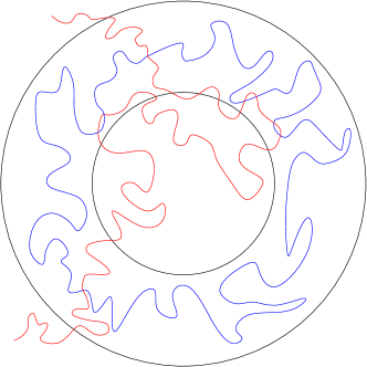
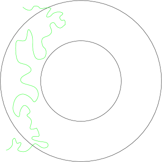
Figure 2: An illustration of a key step of the proof of Lemma 2.19. The idea is that, if an almost geodesic crosses an annulus, then we can bound the distance across the annulus from above in terms of the length of the path inside the region bounded by the inner circle. We do this by “rerouting” $P$ along a path around the annulus to avoid the region bounded by the inner circle. Left: The path $P$ (red) between $z$ and $w$, whose length is at most $D(z,w)+\delta(\varepsilon)$, hits the circle $\partial B_{r_{j}}(x)$ between two times that it hits $\partial B_{2r_{j}}(x)$. Therefore, given a path $\widetilde{P}$ (blue) around the annulus $\mathbbm{A}_{r_{j},2r_{j}}(x)$, Right: we can construct a new path (green) from $z$ to $w$ whose length is at most $\operatorname{len}(\widetilde{P})+\operatorname{len}(P\cap B_{r_{j}}(x)^{c})$. This implies that the distance around the annulus is bounded below by $\operatorname{len}(P\cap B_{r_{j}}(x))-\delta(\varepsilon)$.

Now, observe that if $\widetilde{P}$ is any path around $\mathbbm{A}_{r_{j},2r_{j}}(x)$, then we can use $\widetilde{P}$ to construct a new path from $z$ to $w$ that avoids $B_{r_{j}}(x)$ entirely, and whose length is at most $\operatorname{len}(\widetilde{P})+\operatorname{len}(P\cap B_{r_{j}}(x)^{c})$. (See Figure 2.) Therefore, for each $j\in[1,N]_{\mathbbm{Z}}$,

$$D(z,w)\leq D(\text{around $\mathbbm{A}_{r_{j},2r_{j}}(x)$})+\operatorname{len}(P\cap B_{r_{j}}(x)^{c}).$$

Since $\operatorname{len}(P;D)\leq D(z,w)+\delta(\varepsilon)$, we deduce that, for each $j\in[1,N]_{\mathbbm{Z}}$,

$$\operatorname{len}(P;D)\leq D(\text{around $\mathbbm{A}_{r_{j},2r_{j}}(x)$})+\operatorname{len}(P\cap B_{r_{j}}(x)^{c})+\delta(\varepsilon)$$

and therefore

$$D(\text{around $\mathbbm{A}_{r_{j},2r_{j}}(x)$})\geq\operatorname{len}(P\cap B_{r_{j}}(x))-\delta(\varepsilon)\geq\sum_{i=1}^{j}D(\text{across $\mathbbm{A}_{r_{i}/2,r_{i}}(x)$})-\delta(\varepsilon).$$

By (2.21) for $j=1$ and a Gaussian tail bound, we can choose $\delta(\cdot)$ deterministically such that $\delta(\varepsilon)<\frac{1}{2}D(\text{across $\mathbbm{A}_{r_{1}/2,r_{1}}(x)$})$ on an event $\mathcal{F}^{*}\subset\mathcal{F}$ with probability $1-O_{\varepsilon}(\varepsilon^{q})$ (also at a rate uniform in $x\in K$). From now on, we work on the event $\mathcal{F}^{*}$. We have

$$D(\text{around $\mathbbm{A}_{r_{j},2r_{j}}(x)$})\geq\frac{1}{2}\sum_{i=1}^{j}D(\text{across $\mathbbm{A}_{r_{i}/2,r_{i}}(x)$})\qquad\forall j\in[1,N]_{\mathbbm{Z}}.$$

Combining this inequality with (2.17) and (2.18) yields

$$D(\text{across $\mathbbm{A}_{r_{j}/2,r_{j}}(x)$})\geq\frac{1}{2C^{2}}\sum_{i=1}^{j}D(\text{across $\mathbbm{A}_{r_{i}/2,r_{i}}(x)$})\qquad\forall j\in[1,N]_{\mathbbm{Z}}.$$

We now set $x_{j}=D(\text{across $\mathbbm{A}_{r_{j}/2,r_{j}}(x)$})$ for $j\in[1,N]_{\mathbbm{Z}}$ and apply Lemma 2.20. We get

$$N=\#\mathopen{}\mathclose{{}\left\{j:x_{j}>\frac{1}{2C^{2}}\sum_{i=1}^{j}x_{i}}\right\}\leq\frac{1}{\log(1+1/(2C^{2}))}\log\mathopen{}\mathclose{{}\left(\frac{1}{x_{1}}\max_{j\in[1,N]_{\mathbbm{Z}}}x_{j}}\right)+2.$$

Since $\max_{j\in[1,N]_{\mathbbm{Z}}}x_{j}\leq\operatorname{len}(P)$, this implies

$$N\leq c+\frac{1}{\log(1+1/(2C^{2}))}\log(1/x_{1})$$ (2.22)

for some constant $c>0$ that does not depend on $\varepsilon$. Now, (2.21) yields

$$\frac{1}{x_{1}}\leq Cr_{1}^{-\xi\mathopen{}\mathclose{{}\left(Q+\lambda-\frac{h_{r_{1}}(x)}{\log r_{1}^{-1}}}\right)}$$

Plugging this into (2.22) and using the fact that $N\geq C^{-1}\log r_{1}^{-1}$, we obtain

$$C^{-1}\log r_{1}^{-1}\leq c+\frac{\xi}{\log(1+1/(2C^{2}))}\mathopen{}\mathclose{{}\left(Q+\lambda-\frac{h_{r_{1}}(x)}{\log r_{1}^{-1}}}\right)\log r_{1}^{-1}$$

for some constant $c>0$ that do not depend on $\varepsilon$. We conclude that, on the event $\mathcal{F}^{*}$,

$$\frac{h_{r_{1}}(x)}{\log r_{1}^{-1}}\leq Q+\lambda-\frac{\log(1+1/(2C))}{C\xi}$$ (2.23)

The result follows from taking $\varepsilon$ sufficiently small so that the right-hand side of (2.23) is less than $Q$. ∎

From Lemma 2.19, we deduce that $D$-geodesic segments in small Euclidean neighborhoods must indeed have small $D$-length:

Lemma 2.21.

Suppose we are in the setting of Lemma 2.19, and suppose that $D$ is a complete metric on $U\backslash\{\text{singular points}\}$. Let $z,w\in K\subset U$ for some compact set $K$, and let $P$ be a path from $z$ to $w$ in $K$ with $D$-length at most $D(z,w)+\delta$ for some $\delta\geq 0$. Then a.s.

$$\limsup_{\varepsilon\rightarrow 0}\sup_{y\in K}\operatorname{len}(P\cap B_{\varepsilon}(y))\leq\delta$$

Proof.

Assume that $0<\varepsilon<|z-w|/8$. Let $t_{z}^{\varepsilon}$ denote the last exit of $P$ from $B_{4\varepsilon}(z)$, and $t_{w}^{\varepsilon}$ the first entry of $P$ into $B_{4\varepsilon(w)}$. We will show that, with probability tending to $1$ as $\varepsilon\rightarrow 0$,

$$\operatorname{len}(P\cap B_{\varepsilon^{2}/2}(y))\leq\max\{\operatorname{len}(P[0,t_{z}^{\varepsilon}]),\operatorname{len}(P[t_{w}^{\varepsilon},T]),C\varepsilon^{b}+\delta\}$$ (2.24)

where $C=C(1,3)>1$ is as in Lemma 2.17 and $b$ is some positive constant. To see why this implies the statement of the lemma, note that in the $\varepsilon\rightarrow 0$ limit, the left-hand side of (2.24) is nonincreasing, and the right-hand side is a.s. converging to $\delta$ by the completeness assumption on $D$. So, to prove that $\operatorname{len}(P\cap B_{\varepsilon}(y))\rightarrow 0$ a.s. as $\varepsilon\rightarrow 0$, it is enough to show that (2.24) holds a.s. for arbitrarily small values of $\varepsilon$, which is true automatically if (2.24) holds with probability tending to $1$ as $\varepsilon\rightarrow 0$.

To prove that (2.24) holds with probability tending to $1$ as $\varepsilon\rightarrow 0$, we first note that $\varepsilon$ is small enough that $B_{3\varepsilon}(y)$ cannot contain both $z$ and $w$. Thus, we have two cases to consider.

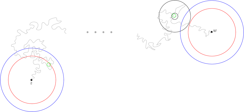
Figure 3: A sketch of the proof of Lemma 2.21. We want to show that, by choosing $\varepsilon>0$ sufficiently small, we can make the $D$-length of the path $P$ (gray) inside the ball $B_{\varepsilon^{2}/2}(y)$ arbitrarily small simultaneously for all choices of $y\in K$. To prove this fact, we choose balls of radius $3\varepsilon$ (boundaries in red) and $4\varepsilon$ (boundaries in blue) centered at the points $z$ and $w$, and we consider separately the cases where $y$ is or is not contained in one of the red balls. (In illustrating both cases, we have colored the boundary of $B_{\varepsilon^{2}/2}(y)$ in green.) If $y$ is in one of the red balls, then $B_{\varepsilon^{2}/2}(y)$ must be contained in the corresponding blue ball, so the parts of the path $P$ in $B_{\varepsilon^{2}/2}(y)$ must have small $D$-length by the completeness property of $D$. If $y$ is not in one of the red balls, then we can choose a point $x$ from a deterministic lattice of $\sim\varepsilon^{-2}$ points such that $B_{\varepsilon^{2}/2}(y)$ is separated from $z,w$ by the annulus $\mathbbm{A}_{\varepsilon^{2},2\varepsilon}(x)$ (black). By a union bound over the deterministic lattice, we can apply Lemma 2.19 to upper bound the $D$-distance around the annulus $\mathbbm{A}_{\varepsilon^{2},2\varepsilon}(x)$. As we showed in Figure 2, we can use this upper bound to derive an upper bound for the $D$-length of $P$ in $B_{\varepsilon^{2}}(x)$ (and therefore in $B_{\varepsilon^{2}/2}(y)$) by “rerouting” the path $P$ to avoid the inner ball $B_{\varepsilon^{2}}(x)$ of the annulus.

Case 1: $B_{3\varepsilon}(y)$ contains exactly one of the points $z,w$.

Suppose that $z\in B_{3\varepsilon}(y)$ and $w\notin B_{3\varepsilon}(y)$. Then $B_{\varepsilon^{2}/2}(y)\subset B_{4\varepsilon}(z)$, and the path $P$ can intersect $B_{\varepsilon^{2}/2}(y)$ only until the last time $t^{\varepsilon}_{z}$ that $P$ exits $B_{4\varepsilon}(z)$. Thus, $\operatorname{len}(P\cap B_{\varepsilon^{2}/2}(y))\leq P([0,t^{\varepsilon}_{z}])$. Similarly, if $w\in B_{3\varepsilon(y)}$ and $z\notin B_{3\varepsilon}(y)$, then $\operatorname{len}(P\cap B_{\varepsilon^{2}/2}(y))\leq\operatorname{len}(P[t^{\varepsilon}_{w},T])$.

Case 2: $B_{3\varepsilon}(y)$ contains neither of the points $z,w$.

Now, suppose that $z,w\notin B_{\varepsilon^{1/2}}(y)$. Since $y$ is random, we cannot apply Lemma 2.19 to $y$ directly; instead, choose $x\in B_{\varepsilon}(K)\cap\mathopen{}\mathclose{{}\left(\frac{\varepsilon^{2}}{4}\mathbbm{Z}^{2}}\right)$ such that $|x-y|<\frac{\varepsilon^{2}}{2}$. Observe that $z,w$ lie outside the ball $B_{2\varepsilon}(x)$. Also, if $P$ intersects the ball $B_{\varepsilon^{2}/2}(y)$, then $P$ must intersect the ball $B_{\varepsilon^{2}}(x)$. By Lemma 2.19 and a union bound, on an event $\mathcal{F}_{\varepsilon}$ with probability tending to $1$ as $\varepsilon\rightarrow 0$, we can find $r\in[\varepsilon^{2},\varepsilon]\cap\{4^{-k}\}_{k\in\mathbbm{N}}$ for which the event $E_{r}(x;C)$ holds and $\frac{h_{r}(x)}{\log r^{-1}}\leq\zeta$, where $\zeta<Q$. Henceforth, we assume that $\mathcal{F}_{\varepsilon}$ occurs. As in the proof of Lemma 2.19, we can use any path $\widetilde{P}$ around $\mathbbm{A}_{r,2r}(x)$ to construct a path from $z$ to $w$ that does not intersect $B_{r}(x)$ and whose length is at most $\operatorname{len}(\widetilde{P})+\operatorname{len}(P\cap B_{r}(x)^{c})$. Therefore

$$\operatorname{len}(P\cap B_{\varepsilon^{2}}(x))\leq D(\text{around $\mathbbm{A}_{r,2r}(x)$})+\delta$$ (2.25)

Since $E_{r}(x;C)$ occurs and $\frac{h_{r}(x)}{\log r^{-1}}\leq\zeta$, (2.25) implies that

$$\operatorname{len}(P\cap B_{\varepsilon^{2}}(x))\leq C\mathfrak{c}_{r}r^{\xi h_{r}(x)}+\delta\leq C\mathfrak{c}_{r}r^{-\xi\zeta}+\delta.$$

Since $\mathfrak{c}_{r}=r^{\xi Q+o_{r}(1)}$ as $r\rightarrow 0$, we can choose $b>0$ such that $\operatorname{len}(P\cap B_{\varepsilon^{2}}(x))\leq Cr^{b}+\delta$ for all $\varepsilon>0$ sufficiently small. Since $B_{\varepsilon^{2}/2}(y)$ is contained in $B_{\varepsilon^{2}}(x)$, we conclude that, if $z,w\notin B_{\varepsilon^{1/2}}(y)$, then, on the event $\mathcal{F}_{\varepsilon}$, we have $\operatorname{len}(P\cap B_{\varepsilon}(y))\leq C\varepsilon^{b}+\delta$. ∎

We can also use Lemma 2.19 to bound from above the thickness of points along $D$-geodesics by some deterministic constant strictly less than $Q$:

Lemma 2.22.

In the setting of Lemma 2.19, there is a deterministic $\zeta<Q$ such that, almost surely, for every geodesic in $U$ and every point $y$ on the geodesic minus its endpoints, we have

$$\liminf_{r\rightarrow 0}\frac{h_{r}(y)}{\log{r^{-1}}}\leq\zeta.$$

Proof.

Let $P$ be a geodesic in $U$, and let $K\subset U$ be a compact set that contains $P$. As in the proof of Lemma 2.21, we cannot apply Lemma 2.19 to a random point $y$ to bound the circle average of the field at $y$. Instead, we will choose $x$ from a deterministic lattice, sufficiently close to $y$ that the circle averages at $x$ and $y$ are probably close in value, and we apply Lemma 2.19 at $x$ to get a bound for the circle average at $x$. Specifically, we first observe that if $y$ is a point on the geodesic $P$ that is at distance greater than $2\varepsilon+\frac{\varepsilon^{2}}{2}$ from the endpoints of $P$, then we can choose $x\in B_{\varepsilon}(K)\cap\mathopen{}\mathclose{{}\left(\frac{\varepsilon^{2}}{4}\mathbbm{Z}^{2}}\right)$ such that $P$ hits $\partial B_{\varepsilon^{2}}(x)$ between two times that it hits $\partial B_{2\varepsilon}(x)$. Now, for fixed $a\in\mathbbm{R}$ and $b\in(0,1/2)$, let $\mathcal{F}_{\varepsilon,a,b}$ be the event that the following two properties hold:

1. For every $x\in B_{\varepsilon}(K)\cap\mathopen{}\mathclose{{}\left(\frac{\varepsilon^{2}}{4}\mathbbm{Z}^{2}}\right)$, if a geodesic hits $\partial B_{\varepsilon^{2}}(x)$ between two times that it hits $\partial B_{2\varepsilon}(x)$, then $h_{r}(x)\leq a\log r^{-1}$ for some $r\in[\varepsilon^{2},\varepsilon]\cap\{4^{-k}\}_{k\in\mathbbm{N}}$.

2. For all $x,y\in K$ with $|x-y|<2r$ and $r\in(0,\varepsilon)$,

   $$|h_{r}(x)-h_{r^{1-b}}(y)|\leq 3\sqrt{10b}\log r^{-1}.$$

By Lemma 2.19 and [GHM20, Lemma 3.15], we can choose $a<Q$ such that, for each choice of $b\in(0,1/2)$, we have $\mathbbm{P}(\mathcal{F}_{\varepsilon,a,b})\rightarrow 1$ as $\varepsilon\rightarrow 0$. Hence, for such $a$ and $b$, it is almost surely the case that $\mathcal{F}_{\varepsilon,a,b}$ holds for arbitrarily small values of $\varepsilon$. On the event $\mathcal{F}_{\varepsilon,a,b}$, every point $y$ on a geodesic $P$ that is at distance greater than $2\varepsilon+\frac{\varepsilon^{2}}{2}$ from the endpoints of $P$ must satisfy $h_{r^{1-b}}(y)\leq(a+3\sqrt{10b})\log r^{-1}$ for some $r\in[\varepsilon^{2},\varepsilon]\cap\{4^{-k}\}_{k\in\mathbbm{N}}$. Since it is a.s. the case that $\mathcal{F}_{\varepsilon,a,b}$ holds for arbitrarily small values of $\varepsilon$, this means that for every point $y$ that lies on some geodesic minus its endpoints, we have $h_{r^{1-b}}(y)\leq(a+3\sqrt{10b})\log r^{-1}$ for arbitrarily small values of $r$ and so

$$\liminf_{r\rightarrow 0}\frac{h_{r}(y)}{\log r^{-1}}\leq\zeta:=\frac{a+3\sqrt{10b}}{1-b}.$$

By choosing $b\in(0,1/2)$ small enough that $\zeta<Q$, we obtain the desired result. ∎

2.5 Proving Axiom II

We now proceed with the proof of Proposition 2.5. Observe that, to prove Proposition 2.5, it is enough to show that $D$ is a.s. determined by $h$, since the statement of Axiom II then follows from the fact that $D$ is a $\xi$-additive local metric. In other words, it suffices to show that, if $D$ and $\widetilde{D}$ are conditionally independent samples from the conditional distribution of $D$ given $h$, then a.s. $D=\widetilde{D}$. We first prove a proposition that implies a weaker result: namely, that $D$ and $\widetilde{D}$ are a.s. bi-Lipschitz equivalent with deterministic Lipschitz constant.

Lemma 2.23 (Bi-Lipschitz equivalence).

Suppose that $(h,D,\widetilde{D})$ is a coupling of $h$ with two random lower semicontinuous metrics $D,\widetilde{D}$ on a connected open set $U\subset\mathbbm{C}$ that are jointly local and $\xi$-additive for $h$ and satisfy Axioms I, IV and V. Then there is a deterministic constant $C$ such that a.s., for any fixed rational circles $O,O^{\prime}$ in $U$,

$$\widetilde{D}(O,O^{\prime})\leq CD(O,O^{\prime}).$$

Proof.

Let $\delta>0$, and let $P:[0,T]\rightarrow U$ be a path (chosen in a measurable manner) from $z$ to $w$ parametrized by $D$-length and whose $D$-length $T$ is at most $D(z,w)+\delta$. We may choose a compact subset $K\subset U$ such that $P\subset K$ on an event $\mathcal{F}^{*}$ with probability $\geq 1-\delta$. By Lemma 2.17, we can choose $C>0$ deterministically such that, on an event $\mathcal{F}\subset\mathcal{F}^{*}$ with probability $1-\delta-O_{\varepsilon}(\varepsilon^{q})$, the following is true. For each $x\in U\cap B_{\varepsilon}(K)\cap\mathopen{}\mathclose{{}\left(\frac{\varepsilon^{2}}{4}\mathbbm{Z}^{2}}\right)$, we can choose $r\in[\varepsilon^{1+m}\mathbbm{r},\varepsilon\mathbbm{r}]$ such that

$$\widetilde{D}(\text{around $\mathbbm{A}_{r,2r}(x)$})\leq CD(\text{across $\mathbbm{A}_{r/2,r}(x)$})$$ (2.26)

For the rest of the proof, we work on the event $\mathcal{F}$.

We now construct a collection of balls $\{B_{r_{j}/2}(x_{j})\}_{j\in[1,J]_{\mathbbm{N}}}$ for some $J\in\mathbbm{N}$, with

$$x_{j}\in U\cap B_{\varepsilon}(K)\cap\mathopen{}\mathclose{{}\left(\frac{\varepsilon^{2}}{4}\mathbbm{Z}^{2}}\right)\qquad\text{and}\qquad r_{j}\in[\varepsilon^{1+m},\varepsilon]\qquad\forall j,$$ (2.27)

such that (2.26) holds with $x=x_{j}$ and $r=r_{j}$ for each $j$. We construct this collection of balls by the following finite inductive procedure:

• First, we choose $x_{1}$ and $r_{1}$ satisfying (2.27) such that $z\in B_{r_{1}/2}(x_{1})$ and such that (2.26) holds with $x=x_{1}$ and $r=r_{1}$. We also set $t_{1}=0$.

• Suppose that we have defined $x_{j}$ and $r_{j}$ for some $j$, and also some time $t_{j}\in[0,T]$. If the ball $B_{r_{j}/2}(x_{j})$ contains the entire segment $P([t_{j},T])$, then we set $j=J$ and the procedure terminates. Otherwise, we let $t_{j+1}$ be the first time after $t_{j}$ that $P$ exits the ball $B_{r_{j}}(x_{j})$, and we choose $x_{j+1}$ and $r_{j+1}$ satisfying (2.27) such that $P(t_{j+1})\in B_{r_{j+1}/2}(x_{j+1})$ and such that (2.26) holds with $x=x_{j+1}$ and $r=r_{j+1}$.

Let $C_{r_{j}}(x_{j})$ be a path that disconnects $\partial B_{r_{j}}(x_{j})$ and $\partial B_{2r_{j}}(x_{j})$ whose $\widetilde{D}$-length is at most $\varepsilon/J$ plus the $\widetilde{D}$-distance around the annulus $\mathbbm{A}_{r_{j},2r_{j}}(x_{j})$. Since the balls $B_{r_{j/2}}(x_{j})$ for $j=[1,J]_{\mathbbm{N}}$ cover $P([0,t_{J}])$, we can deduce from topological considerations (as in [GM19b, Lemma 4.3]) that the union of the paths $C_{r_{j}}(x_{j})$ is connected. Moreover, the union of the paths $C_{r_{j}}(x_{j})$ contains a path from $B_{2\varepsilon}(O)$ to $B_{2\varepsilon}(O^{\prime})$. It follows that, on the event $\mathcal{F}$, the $\widetilde{D}$-distance from $B_{2\varepsilon}(O)$ to $B_{2\varepsilon}(O^{\prime})$ is at most

$$\sum_{j=1}^{J}\operatorname{len}(C_{r_{j}}(x_{j});\widetilde{D}) \leq\sum_{j=1}^{J}\mathopen{}\mathclose{{}\left[\widetilde{D}(\text{around $\mathbbm{A}_{r_{j},2r_{j}}(x_{j})$})+\varepsilon/J}\right]$$

$$\leq\varepsilon+C\sum_{j=1}^{J}D(\text{across $\mathbbm{A}_{r_{j}/2,r_{j}}(x_{j})$})$$

$$\leq\varepsilon+C\sum_{j=1}^{J}(t_{j+1}-t_{j})$$

$$\leq\varepsilon+CT\leq CD(O,O^{\prime})+C\delta.$$

Since $\widetilde{D}$ is lower semicontinuous, sending $\varepsilon\rightarrow 0$ and then $\delta\rightarrow 0$ yields the desired result. ∎

The proof of Proposition 2.5, like its counterpart in the continuous metric setting, involves applying the Efron-Stein inequality. To set up our application of this inequality, we introduce some notation.

Definition 2.24 (Defining a $\theta$-shifted grid of $\varepsilon\times\varepsilon$ squares).

For $\theta\in[0,1]^{2}$, and let $\mathcal{G}_{\theta}$ be the randomly shifted square grid given by the horizontal and vertical lines joining points of $\mathbbm{Z}^{2}+\theta$. We define the set of squares $\mathcal{S}_{\theta}^{\varepsilon}$ as the set of open $\varepsilon\times\varepsilon$ squares given by the connected components of the complement of the rescaled grid $\varepsilon\mathcal{G}_{\theta}$.

We will use this grid of squares, with $\theta$ chosen randomly from Lebesgue measure on $[0,1]^{2}$, to decompose the variance of $D(O,O^{\prime})$ given $h$ and $\theta$, for a pair of rational circles $O,O^{\prime}$, in terms of the metrics $D^{S}$ for $S\in\mathcal{S}_{\theta}^{\varepsilon}$, where $D^{S}$ denotes the new metric obtained by $D$ by resampling $D(\cdot,\cdot;S\cap U)$ from its conditional law given $(h,\theta)$. We will apply the Efron-Stein inequality to write

$$\operatorname{Var}[D(O,O^{\prime})|h,\theta]\leq\frac{1}{2}\sum_{S\in\mathcal{S}_{\theta}^{\varepsilon}}\mathbbm{E}\mathopen{}\mathclose{{}\left[(D^{S}(O,O^{\prime})-D(O,O^{\prime}))^{2}|h,\theta}\right].$$

To justify this application of the Efron-Stein inequality, we require the following two lemmas, which generalize the results stated in [GM19b, Lemmas 5.1-5.4].

Lemma 2.25.

In the setting of Proposition 2.5, we can choose a deterministic $C>0$ such that, for each fixed $V\subset U$ and rational circles $O,O^{\prime}\subset V$, a.s.

$$C^{-1}\mathbbm{E}[D(O,O^{\prime};V)|h]\leq D(O,O^{\prime};V)\leq C\mathbbm{E}[D(O,O^{\prime};V)|h]$$ (2.28)

and

$$\mathbbm{E}[D(O,O^{\prime};V)^{q}|h]<\infty\qquad$$ (2.29)

Moreover, if $(h,D)\overset{d}{=}(h,D^{\prime})$, then a.s. $D,D^{\prime}$ are bi-Lipschitz equivalent with Lipschitz constant $C^{2}$.

Proof.

The proof of (2.28) is identical to the proof of [GM19b, Lemma 5.1] with $z,w$ replaced by $O,O^{\prime}$. The bound (2.29) follows immediately from (2.28). Finally, if $(h,D)\overset{d}{=}(h,D^{\prime})$, then (2.28) implies that

$$C^{-2}D(O,O^{\prime})\leq D^{\prime}(O,O^{\prime})\leq C^{2}D(O,O^{\prime})$$

for all $O,O^{\prime}$; since $D,D^{\prime}$ are lower semicontinuous, this implies that a.s. $D,D^{\prime}$ are bi-Lipschitz equivalent with Lipschitz constant $C^{2}$. ∎

Lemma 2.26.

In the setting of Proposition 2.5, let $\theta$ be sampled uniformly from Lebesgue measure on $[0,1]^{2}$, and let $\mathcal{S}_{\theta}^{\varepsilon}$ be the set of open $\varepsilon\times\varepsilon$ squares in $U$ with side length $1$ and vertices in $\mathbbm{Z}^{2}+\theta$. Then

• For any fixed $\varepsilon>0$ and any path $P$ in $U$ with finite $D$-length chosen in a manner depending only on $h$ and $D$, we have

  $$\operatorname{len}(P;D)=\sum_{S\in\mathcal{S}_{\theta}^{\varepsilon}}\operatorname{len}(P\cap S;D).$$ (2.30)

• The metric $D$ is a.s. determined by $h,\theta$ and the set of internal metrics $\{D(\cdot,\cdot;S\cap U):S\in\mathcal{S}_{\theta}^{\varepsilon}\}$.

• The internal metrics $\{D(\cdot,\cdot;S\cap U):S\in\mathcal{S}_{\theta}^{\varepsilon}\}$ are conditionally independent given $h$ and $\theta$.

Proof.

These three assertions were stated as [GM19b, Lemmas 5.2], [GM19b, Lemmas 5.3] and [GM19b, Lemmas 5.4], respectively, in the case in which $D$ is continuous. The proof of the first and third assertions in that setting apply directly here as well.

To prove the second assertion, we condition on $h,\theta$, and the internal metrics $\{D(\cdot,\cdot;S\cap U):S\in\mathcal{S}_{\theta}^{\varepsilon}\}$, and we consider two conditionally independent samples $D$ and $D^{\prime}$ from the conditional law of $D$. To prove the assertion, it is enough to show that $D=D^{\prime}$ almost surely. Suppose that $O,O^{\prime}$ are fixed rational balls in $U$, and let $P$ be a path from $O$ to $O^{\prime}$, chosen in a manner depending only on $D$. The first assertion of the lemma gives

$$\operatorname{len}(P;D)=\sum_{S\in\mathcal{S}_{\theta}^{\varepsilon}}\operatorname{len}(P\cap S;D)\qquad\text{a.s.}$$

Combined with (2.28) of Lemma 2.25, this implies

$$\operatorname{len}(P;D^{\prime})=\sum_{S\in\mathcal{S}_{\theta}^{\varepsilon}}\operatorname{len}(P\cap S;D^{\prime})\qquad\text{a.s.}$$

Since the internal metrics of $D$ and $D^{\prime}$ on $S\cap U$ agree for each $S\in\mathcal{S}_{\theta}^{\varepsilon}$, we deduce that $P$ has the same length in the metrics $D$ and $D^{\prime}$. Thus, a.s. $D(O,O^{\prime})=D^{\prime}(O,O^{\prime})$. Since $D,D^{\prime}$ are lower semicontinuous, this implies that $D=D^{\prime}$ a.s., proving the second assertion of the lemma. ∎

We now prove Proposition 2.5 in a manner analogous to [GM19b, Theorem 1.7]. They key difference in our proof is the application of Lemma 2.21 to control the length of $P$ in a small square. Observe that, in contrast to the proof  [GM19b, Theorem 1.7], our proof requires the introduction of the second small parameter $\delta>0$.

Proof of Proposition 2.5.

As noted at the beginning of this section, it suffices to prove that $D$ is a.s. determined by $h$, since Axiom II then follows from the fact that $D$ is a $\xi$-additive local metric.

First, since $D$ is almost surely determined by the internal metric $D(\cdot,\cdot;V)$ for bounded and connected subsets $V\subset U$, it is enough to prove the result for $U$ a bounded and connected open set. As in the proof of Lemma 2.25, it suffices to show that, for each fixed pair of rational circles $O,O^{\prime}\subset U$, the quantity $D(O,O^{\prime})$ is a.s. determined by $h$.

By Lemma 2.26, $D$ is a.s. determined by its internal metrics on the squares $S\in\mathcal{S}_{\theta}^{\varepsilon}$, and these internal metrics are conditionally independent given $h$. Thus, by the Efron-Stein inequality, if we let $D^{S}$ denote the new metric obtained by $D$ by resampling $D(\cdot,\cdot;S\cap U)$ from its conditional law given $(h,\theta)$, then

$$\operatorname{Var}[D(O,O^{\prime})|h,\theta]\leq\frac{1}{2}\sum_{S\in\mathcal{S}_{\theta}^{\varepsilon}}\mathbbm{E}\mathopen{}\mathclose{{}\left[(D^{S}(O,O^{\prime})-D(O,O^{\prime}))^{2}|h,\theta}\right].$$ (2.31)

Since $(h,D^{S})\overset{d}{=}(h,D)$, the law of $D^{S}(O,O^{\prime})-D(O,O^{\prime})$ is symmetric about the origin, and so $\mathbbm{E}\mathopen{}\mathclose{{}\left[(D^{S}(O,O^{\prime})-D(O,O^{\prime}))^{2}|h,\theta}\right]=2\mathbbm{E}\mathopen{}\mathclose{{}\left[(D^{S}(O,O^{\prime})-D(O,O^{\prime}))_{+}^{2}|h,\theta}\right]$, where $x_{+}=\max\{x,0\}$. Hence, we can rewrite the inequality (2.31) as

$$\operatorname{Var}[D(O,O^{\prime})|h,\theta]\leq\sum_{S\in\mathcal{S}_{\theta}^{\varepsilon}}\mathbbm{E}\mathopen{}\mathclose{{}\left[(D^{S}(O,O^{\prime})-D(O,O^{\prime}))_{+}^{2}|h,\theta}\right].$$ (2.32)

Since $(h,D^{S})\overset{d}{=}(h,D)$, Lemma 2.25 implies that we can choose a deterministic $C>0$ such that a.s.

$$C^{-2}D(O,O^{\prime})\leq D^{S}(O,O^{\prime})\leq C^{2}D(O,O^{\prime})\qquad\forall z,w\in U.$$ (2.33)

Fix $\delta>0$, and let $P$ be a fixed path from $O$ to $O^{\prime}$ that depends only on $(h,D)$ with $D$-length at most $D(O,O^{\prime})+\delta$. For each $S^{\prime}\in\mathcal{S}_{\theta}^{\varepsilon}$ different from $S$, the $D^{S}$-length and $D$-length of $P\cap S^{\prime}$ agree. Thus, (2.30) of Lemma 2.26 combined with (2.33) gives

$$C^{-2}\operatorname{len}(P\cap S;D)\leq\operatorname{len}(P\cap S;D^{S})\leq C^{2}\operatorname{len}(P\cap S;D).$$ (2.34)

As in the proof of the second assertion of Lemma 2.26, this implies that

$$\operatorname{len}(P;D^{S})=\sum_{S^{\prime}\in S_{\theta}^{\varepsilon}}\operatorname{len}(P\cap S^{\prime};D^{S})$$

By (2.34), the latter is at most $D(O,O^{\prime})+C^{2}\operatorname{len}(P\cap S;D)$. Therefore, a.s.

$$(D^{S}(O,O^{\prime})-D(O,O^{\prime}))_{+}\leq C^{2}\operatorname{len}(P\cap S;D)+\delta^{2}.$$

Plugging this into (2.32) and applying the Cauchy-Schwartz inequality yields

$$\operatorname{Var}[D(O,O^{\prime})|h,\theta] \leq\mathbbm{E}\mathopen{}\mathclose{{}\left[\sum_{S^{\prime}\in\mathcal{S}_{\theta}^{\varepsilon}}(C^{2}\operatorname{len}(P\cap S;D)+\delta)^{2}|h,\theta}\right]$$

$$\leq 2C^{4}\mathbbm{E}\mathopen{}\mathclose{{}\left[\sum_{S^{\prime}\in\mathcal{S}_{\theta}^{\varepsilon}}\operatorname{len}(P\cap S;D)\mathopen{}\mathclose{{}\left(\max_{S\in\mathcal{S}_{\theta}^{\varepsilon}}\operatorname{len}(P\cap S;D)}\right)|h,\theta}\right]+2\delta^{2}\#\mathcal{S}_{\theta}^{\varepsilon}$$

$$\leq 2C^{4}\mathbbm{E}\mathopen{}\mathclose{{}\left[(D(O,O^{\prime}))^{2}|h,\theta}\right]^{1/2}\mathbbm{E}\mathopen{}\mathclose{{}\left[\mathopen{}\mathclose{{}\left(\max_{S\in\mathcal{S}_{\theta}^{\varepsilon}}\operatorname{len}(P\cap S;D)}\right)^{2}|h,\theta}\right]^{1/2}+2\delta^{2}\#\mathcal{S}_{\theta}^{\varepsilon}$$

By Lemma 2.25, the quantity $\mathbbm{E}\mathopen{}\mathclose{{}\left[(D(O,O^{\prime}))^{2}|h,\theta}\right]^{1/2}$ is finite almost surely. Moreover, by Lemma 2.21,

$$\limsup_{\varepsilon\rightarrow 0}\max_{S\in\mathcal{S}_{\theta}^{\varepsilon}}\operatorname{len}(P\cap S;D)\leq\delta\qquad\text{a.s.}.$$

Since $\operatorname{len}(P\cap S;D)\leq D(O,O^{\prime})+\delta$ for all $S$, the bounded convergence theorem gives

$$\limsup_{\varepsilon\rightarrow 0}\mathbbm{E}\mathopen{}\mathclose{{}\left[\mathopen{}\mathclose{{}\left(\max_{S\in\mathcal{S}_{\theta}^{\varepsilon}}\operatorname{len}(P\cap S;D)}\right)^{2}|h,\theta}\right]^{1/2}\leq\delta\qquad\text{a.s.}$$

Therefore a.s. $\operatorname{Var}[D(O,O^{\prime})|h,\theta]\rightarrow 0$ as $\varepsilon\rightarrow 0$ and then $\delta\rightarrow 0$, so $D(O,O^{\prime})$ is a.s. determined by $h$, as desired. ∎

We can now check that subsequential limits of the rescaled $\varepsilon$-LFPP metrics (1.3) satisfy Axiom II.

Proof of Lemma 2.6.

In the special case in which $h$ is a whole-plane GFF normalized so that $h_{1}(0)=0$, the result follows from combining Propositions 2.4 and 2.5. For general $h$, let $V,W$ be bounded open sets with $\overline{V}\subset W$ and $\overline{W}\subset U$. By Lemma 2.16, for each $x\in\overline{V}$, we can choose $R_{x}\in\sigma\mathopen{}\mathclose{{}\left(h|_{U}}\right)$ such that $\mathfrak{a}_{\varepsilon_{n}}^{-1}{\widehat{D}^{\varepsilon_{n}}}_{h}(\cdot,\cdot;W)$ converges a.s. to $D_{h}(\cdot,\cdot;W)$ on $B_{R_{x}}(x)$. Therefore, $h|_{U}$ a.s. determines the pair $(R_{x},\mathfrak{a}_{\varepsilon}^{-1}D_{h}(\cdot,\cdot;W)|_{B_{R_{x}}(x)})\in\sigma\mathopen{}\mathclose{{}\left(h|_{U}}\right)$. Since we can cover $\overline{V}$ by finitely many such balls $B_{R_{x}}(x)$, we deduce that $h|_{U}$ a.s. determines the internal metric $D_{h}(\cdot,\cdot;W)$ on $V$. Letting $V$ and $W$ increase to all of $U$ proves the lemma. ∎

2.6 Completing the proof of Theorem 1.7

To complete the proof of Theorem 1.7, we show that we can choose a subsequence $\varepsilon_{n}\rightarrow 0$ for which LFPP distances between pairs of rational circles converge a.s. to the corresponding $D_{h}$-distances.

Lemma 2.27.

For every sequence of values of $\varepsilon$ tending to zero as $\varepsilon\rightarrow 0$, we can choose a subsequence $\varepsilon_{n}$ for which $a_{\varepsilon}^{-1}D^{\varepsilon}_{h}(O,O^{\prime})\rightarrow D_{h}(O,O^{\prime})$ a.s. for all pairs of rational circles $O,O^{\prime}$.

We note that Lemma 2.27 was proved in [DG20, Theorem 1.2] in the special case in which $h$ is a whole-plane GFF and the rational circles are points in $\mathbbm{Q}^{2}$.

Proof.

By Proposition 2.1, it suffices to consider the case in which $h$ is a whole-plane GFF. Moreover, by Lemmas 2.6 and 2.7, it is enough to show that the convergence of distances occurs in law.

By [DG20, Equation 5.1], for every sequence of $\varepsilon$-values tending to zero, we can choose a subsequence $\varepsilon_{n}\rightarrow 0$ along with we have the following joint convergence in law as $n\rightarrow\infty$:

$$\mathfrak{a}_{\varepsilon_{n}}^{-1}D_{h}^{\varepsilon_{n}}(O_{1},O_{2})\rightarrow\mathring{D}_{h}(O_{1},O_{2})\qquad\text{for all rational circles $O_{1},O_{2}$}$$ (2.35)

for some random variables $\mathring{D}_{h}(O_{1},O_{2})$. (Note that $\mathring{D}_{h}$ is not defined as a metric.) By the Skorohod representation theorem, we may couple the random variables in (2.35) so that the convergence occurs almost surely. Thus, to prove the lemma, it suffices to show that in this coupling, a.s.

$$D_{h}(O,O^{\prime})=\mathring{D}_{h}(O,O^{\prime})\qquad\text{for all pairs of rational circles $O,O^{\prime}$}$$ (2.36)

The inequality $D_{h}(O,O^{\prime})\leq\mathring{D}_{h}(O,O^{\prime})$ follows directly from the definition of the lower semicontinuous topology. For the converse inequality, let $z\in O$ and $w\in O^{\prime}$ be such that $D_{h}(z,w)=D_{h}(O,O^{\prime})$. By definition of the lower semicontinuous topology, we can choose sequence of points $z_{n}\rightarrow z$ and $w_{n}\rightarrow w$ with $D_{h}(z,w)=\lim_{n\rightarrow\infty}a_{\varepsilon_{n}}^{-1}D_{h}^{\varepsilon_{n}}(z_{n},w_{n})$. By [DG20, Lemma 5.12], we can choose a deterministic constant $C>0$ and nested sequences $O_{z}^{n}\ni z_{n}$ and $O_{w}^{n}\ni w_{n}$ of rational circles with positive radii that shrink to $z$ and $w$, respectively, such that the following is true. Let $\hat{O}_{z}^{n}$ denote the rational circle with the same center as $O_{z}^{n}$ and twice the radius, and let $A_{z}^{n}$ denote the annulus bounded by $O_{z}^{n}$ and $\hat{O}_{z}^{n}$. We define $\hat{O}_{w}^{n}$ and $A_{w}^{n}$ analogously. Then a.s.

$$\lim_{n\rightarrow\infty}\mathring{D}_{h}(\text{around $A^{n}_{z}$})=\lim_{n\rightarrow\infty}\mathring{D}_{h}(\text{around $A^{n}_{w}$})=0.$$

Also, by [DG20, Lemma 5.18],

$$\lim_{n\rightarrow\infty}\mathring{D}_{h}(z,\hat{O}_{z}^{n})=\lim_{n\rightarrow\infty}\mathring{D}_{h}(w,\hat{O}_{w}^{n})=0.$$

Now, applying [DG20, Lemma 5.2, Assertion (ii)] twice yields the pair of inequalities

$$\mathring{D}_{h}(z,O_{w}^{n})\leq\mathring{D}_{h}(O_{z}^{n},O_{w}^{n})+\mathring{D}_{h}(z,\hat{O}_{z}^{n})+\mathring{D}_{h}(\text{around $A^{m}_{z}$})$$

and

$$\mathring{D}_{h}(z,w)\leq\mathring{D}_{h}(z,O_{w}^{n})+\mathring{D}_{h}(w,\hat{O}_{w}^{n})+\mathring{D}_{h}(\text{around $A^{m}_{w}$}).$$

Combining these two inequalities and taking the $n\rightarrow\infty$ limit, we get

$$\mathring{D}_{h}(z,w)\leq\lim_{n\rightarrow\infty}\mathring{D}_{h}(z,O_{w}^{n})\leq\lim_{n\rightarrow\infty}\mathring{D}_{h}(O_{z}^{n},O_{w}^{n})=D_{h}(z,w).$$

Since $\mathring{D}_{h}(O,O^{\prime})\leq\mathring{D}_{h}(z,w)$, this proves $\mathring{D}_{h}(O,O^{\prime})\leq D_{h}(O,O^{\prime})$. ∎

Proof of Theorem 1.7.

By Proposition 2.1, for every sequence of values of $\varepsilon$ tending to zero, we can find a subsequence $\varepsilon_{n}$ for which the weak limit (2.1) exists. By combining Propositions 2.1 and 2.4 and Lemma 2.6, we conclude that each subsequential limiting metric $D_{h}$ satisfies the five axioms in Definition 1.6 of a weak LQG metric. Moreover, Axiom II and Lemma 2.7 together imply that the convergence (2.1) occurs almost surely. Finally, Lemma 2.27 gives the desired a.s. convergence of distances between pairs of rational circles, and (1.8) is satisfied by our definition of $\mathfrak{c}_{r}$ in the proof of Proposition 2.4.

To complete the proof of the theorem, we now extend the definition of $D_{h}$ to the case of a whole-plane GFF $h$ plus an unbounded continuous function $f$, so that we have a well-defined weak LQG metric $h\mapsto D_{h}$. For each open and bounded subset $V\subset\mathbbm{C}$, we set $D_{h+f}^{V}:=D_{h+\phi_{V}f}(\cdot,\cdot;V)$, where $\phi_{V}$ is a smooth compactly supported bump function which is identically equal to 1 on $V$. By applying Axiom II in the setting of a whole-plane GFF plus a bounded continuous function, we deduce that the metric $D_{h+f}^{V}$ is a.s. determined by $(h+\phi_{V}f)|_{V}=(h+f)|_{V}$, in a manner which does not depend on $\phi_{V}$. We define the metric $D_{h+f}$ as the length metric such that, if $P$ is a continuous path in $\mathbbm{C}$, its $D_{h+f}$-length is equal to its $D_{h+f}^{V}$-length, where $V\subset\mathbbm{C}$ is a bounded open set that contains $P$. The We define $D_{h+f}(z,w)$ for $z,w\in\mathbbm{C}$ to be the infimum of the $D_{h+f}$-lengths of continuous paths from $z$ to $w$. Then $D_{h+f}$ is a length metric on $\mathbbm{C}$ which is a.s. determined by $D_{h+f}$ and which satisfies $D_{h+f}(\cdot,\cdot;V)=D_{h+f}^{V}$ for each bounded open set $V\subset\mathbbm{C}$. It is easy to check that $D_{h+f}$ satisfies the axioms in Definition 1.6, so that the mapping $h\mapsto D_{h}$ is a weak $\gamma$-LQG metric, as desired. ∎

3 Properties of weak LQG metrics

Throughout this and the next section, we let $h$ be a whole-plane GFF plus a continuous function (unless specified otherwise), and we let $D_{h}$ be the metric associated to $h$ by a weak LQG metric $h\mapsto D_{h}$. Our main building blocks for proving properties of $D_{h}$ are Propositions 1.8 and 1.9, which are proven exactly as in the continuous metric setting:

Proof of Proposition 1.8.

This property was stated in the continuous metric setting as [DFG⁺20, Proposition 3.1], and we can apply the proof of that proposition to the supercritical setting without any modifications, except that we apply Lemma 2.17 instead of [DFG⁺20, Lemma 3.2] and define the events $E_{r}(x;C)$ as we did before stating Lemma 2.17. ∎

Proof of Proposition 1.9.

First, (1.7) implies that we can choose a constant $C>1$ such that $C^{-1}\leq\mathfrak{c}_{r^{\prime}}/\mathfrak{c}_{r}\leq C$ whenever $1/2\leq r^{\prime}/r\leq 2$. Thus, in proving (1.10), we may restrict to values of $\delta$ and $r$ of the form $2^{k}$ for $k\in\mathbbm{Z}$. With this restriction, we can directly apply the proof of [DFG⁺20, Theorem 1.5] in the continuous metric setting. The only step we need to modify is the justification of equation (3.19) in the proof of [DFG⁺20, Lemma 3.6]. A version of this statement is proven in [DG20, Lemma 2.11]. Though the discrete LFPP metric in [DG20, Lemma 2.11] is defined slightly differently, the metrics are the same (up to grid rescaling) since the corresponding discrete Gaussian free fields have the same covariance structure. Also, the lemma was stated for the distance across an annulus, but the proof of the lemma applies to the distance between two sides of a square as well. ∎

We can apply Proposition 1.8 directly to prove the following tightness result for distances between compact sets.

Lemma 3.1.

If $U\subset\mathbbm{C}$ is open and $K_{1},K_{2}\subset U$ are connected, disjoint compact sets (that are allowed to be singletons), then the laws of

$$\mathfrak{c}_{r}^{-1}e^{-\xi h_{r}(0)}D_{h}(rK_{1},rK_{2};rU)\quad\text{and}\quad\mathopen{}\mathclose{{}\left(\mathfrak{c}_{r}^{-1}e^{-\xi h_{r}(0)}D_{h}(rK_{1},rK_{2};rU)}\right)^{-1}$$ (3.1)

for varying $r$ are tight.

One immediate consequence of Lemma 3.1 is that the $D_{h}$-distance between two fixed points is a.s.  finite.

Our proof of Lemma 3.1 uses the following elementary lemma for lower semicontinuous metrics:

Lemma 3.2.

Let $D$ be a lower semicontinuous metric on a set $U\subset\mathbbm{C}$. For every $X\subset U$, we have ${\operatorname{diam}}(X;D)={\operatorname{diam}}(\overline{X};D)$, where $\overline{X}$ is the closure of $X$ in the Euclidean topology on $U$.

Proof.

If $z,w\in\overline{X}$, then we can choose sequences $z_{n},w_{n}$ of points in $X$ with $z_{n}\rightarrow z$ and $w_{n}\rightarrow w$. Since $D$ is lower semicontinuous, $D(z,w)\leq\liminf_{n\rightarrow\infty}D(z_{n},w_{n})\leq{\operatorname{diam}}(X;D)$. ∎

Proof of Lemma 3.1.

If $K_{1}$ and $K_{2}$ are not singletons, then the result follows immediately from Proposition 1.8 and Axiom 1.6. To prove the result with $K_{1}$ and $K_{2}$ allowed to be singletons, it suffices to show that, for each fixed $p\in(0,1)$, we can choose $N\in\mathbbm{N}$ and $C>0$ large enough so that, for each $\mathbbm{r}>0$, it is the case with probability at least $1-p$ that

$$C^{-1}\leq D_{h}(\mathbbm{r}z,\partial B_{2^{-N}\mathbbm{r}}(\mathbbm{r}z))\leq C.$$ (3.2)

By Axiom 1.6, we may assume without loss of generality that $h$ is a whole-plane GFF normalized so that $h_{1}(0)=0$.

To prove the bounds (3.2), we first choose some value of $\zeta\in(0,Q/3)$ which will remain fixed. By Proposition 1.8, it holds with superexponentially high probability as $n\rightarrow\infty$, at a rate uniform in $\mathbbm{r}>0$, that

$$2^{-\xi\zeta n}\leq\mathfrak{c}_{2^{-n}\mathbbm{r}}^{-1}e^{-\xi h_{2^{-n}\mathbbm{r}}(\mathbbm{r}z)}D_{h}(\text{across $\mathbbm{A}_{2^{-n}\mathbbm{r},2^{-n+2}\mathbbm{r}}(\mathbbm{r}z)$})\leq 2^{\xi\zeta n}$$ (3.3)

and

$$2^{-\xi\zeta n}\leq\mathfrak{c}_{2^{-n}\mathbbm{r}}^{-1}e^{-\xi h_{2^{-n}\mathbbm{r}}(\mathbbm{r}z)}D_{h}(\text{around $\mathbbm{A}_{2^{-n}\mathbbm{r},2^{-n+1}\mathbbm{r}}(\mathbbm{r}z)$})\leq 2^{\xi\zeta n}.$$ (3.4)

Now, from (1.10) and Markov’s inequality we deduce that, for each $a>0$,

$$\mathbbm{P}\mathopen{}\mathclose{{}\left(2^{-\xi(Q+\zeta)n}\leq\frac{\mathfrak{c}_{2^{-n}\mathbbm{r}}}{\mathfrak{c}_{\mathbbm{r}}}\leq 2^{-\xi(Q-\zeta)n}}\right)\geq 1-2^{-an+o_{n}(n)},$$ (3.5)

where the $o_{n}(n)$ does not depend on $\mathbbm{r}$. Moreover, the Gaussian tail bound [DFG⁺20, Equation (3.8)] yields

$$\mathbbm{P}\mathopen{}\mathclose{{}\left[|h_{2^{-n}\mathbbm{r}}(\mathbbm{r}z)-h_{\mathbbm{r}}(0)|\leq\zeta n\log 2}\right]\geq 1-O_{n}\mathopen{}\mathclose{{}\left(2^{-\zeta^{2}n/2}}\right),$$ (3.6)

where this lower bound does not depend on $\mathbbm{r}$. Combining (3.5) and (3.6) with the bounds (3.3) and (3.4), we deduce that it holds with exponentially high probability as $n\rightarrow\infty$, at a rate uniform in $\mathbbm{r}>0$, that

$$2^{-\xi(Q+3\zeta)n}\leq\mathfrak{c}_{\mathbbm{r}}^{-1}e^{-\xi h_{\mathbbm{r}}(0)}D_{h}(\text{across $\mathbbm{A}_{2^{-n}\mathbbm{r},2^{-n+2}\mathbbm{r}}(\mathbbm{r}z)$})\leq 2^{-\xi(Q-3\zeta)n}$$ (3.7)

and

$$2^{-\xi(Q+3\zeta)n}\leq\mathfrak{c}_{\mathbbm{r}}^{-1}e^{-\xi h_{\mathbbm{r}}(0)}D_{h}(\text{around $\mathbbm{A}_{2^{-n}\mathbbm{r},2^{-n+1}\mathbbm{r}}(\mathbbm{r}z)$})\leq 2^{-\xi(Q-3\zeta)n}.$$ (3.8)

It follows that, for each fixed $p\in(0,1)$, we can choose $N\in\mathbbm{N}$ large enough so that, for each $\mathbbm{r}>0$, it is the case with probability at least $1-p$ that the distance bounds (3.7) and (3.8) hold for all $n\geq N$.

We can now prove the desired bounds (3.2) by iterating the bounds (3.7) and (3.8) across concentric annuli:

• Observe that every path across the annulus $\mathbbm{A}_{2^{-n}\mathbbm{r},2^{-n+2}\mathbbm{r}}(\mathbbm{r}z)$ intersects both every path around $\mathbbm{A}_{2^{-n+1}\mathbbm{r},2^{-n+2}\mathbbm{r}}(\mathbbm{r}z)$ and every path around $\mathbbm{A}_{2^{-n}\mathbbm{r},2^{-n+1}\mathbbm{r}}(\mathbbm{r}z)$. Thus, we can string together paths across the annuli $\mathbbm{A}_{2^{-n}\mathbbm{r},2^{-n+2}\mathbbm{r}}(\mathbbm{r}z)$ and paths around the annuli $\mathbbm{A}_{2^{-n}\mathbbm{r},2^{-n+1}\mathbbm{r}}(\mathbbm{r}z)$ to obtain a path from $\partial B_{2^{-N}\mathbbm{r}}(\mathbbm{r}z)$ to an arbitrarily small neighborhood of $\mathbbm{r}z$. Therefore, we can apply the upper bounds in (3.7) and (3.8) on distances around and across annuli to bound from above the distance from $\partial B_{2^{-N}\mathbbm{r}}(\mathbbm{r}z)$ to an arbitrarily small neighborhood of $\mathbbm{r}z$. By Lemma 3.2, this yields an upper bound for the distance from $\partial B_{2^{-N}\mathbbm{r}}(\mathbbm{r}z)$ to $\mathbbm{r}z$.

• Since every path from $\mathbbm{r}z$ to $\partial B_{2^{-N}\mathbbm{r}}(\mathbbm{r}z)$ must cross the annuli $\mathbbm{A}_{2^{-n}\mathbbm{r},2^{-n+2}\mathbbm{r}}(\mathbbm{r}z)$ for all $n\geq N+2$, we can sum the lower bound in (3.7) over all $n\geq N+2$ to obtain the desired lower bound in (3.2).

∎

3.1 Bounding distances across scales: square annuli and hashes

Proposition 1.8 gives an a.s. distance estimate for distances near a fixed point at varying scales. However, to prove properties of $D_{h}$, we need estimates on distances throughout a fixed bounded region of the plane. To obtain the estimates we need, we partition the region of interest into dyadic squares.

Definition 3.3.

For $n\in\mathbbm{Z}$ and a Borel set $X$, let $\mathcal{S}^{n}(X)$ denote the set of squares of the form $[a,a+2^{-n}]\times[b,b+2^{-n}]$ intersecting $X$ with $a,b\in 2^{-n}\mathbbm{Z}$. When $X$ is a singleton $\{x\}$, we will denote $\mathcal{S}^{n}(\{x\})$ simply by $\mathcal{S}^{n}(x)$.

We write $\mathcal{S}^{n}=\mathcal{S}^{n}(\mathbbm{C})$, and we call $S$ a dyadic square if $S\in\mathcal{S}^{n}$ for some integer $n$. We can decompose every dyadic square $S$ into four squares with side length $|S|/2$; we call these four squares the dyadic children of $S$, and $S$ their dyadic parent.

For a fixed bounded open set in the plane, we will prove two distances bounds that hold a.s. for every sufficiently small dyadic square $S$ intersecting the fixed set: a lower bound on the distance across a square annulus that surrounds $S$, and a upper bound on the diameter of a network of four paths in $S$ that criss-cross $S$. The reason for considering these two sets in particular is that they satisfy several geometric properties that allow us to string together upper and lower distance bounds across scales.

We begin by defining both of these sets and stating their useful geometric properties. (We will not formally prove these properties; they are all easy to see by inspection of Figure 4.)

Lemma 3.4 (The square annulus associated to a dyadic square).

For a square $S$, let $A_{S}$ denote the square annulus centered at $v_{S}$ formed by squares with side lengths $2|S|$ and $3|S|$. These annuli satisfy the following properties:

1. If $S^{\prime}$ is a dyadic child of $S$, then $A_{S^{\prime}}$ is nested in and disjoint from $A_{S}$.

2. If $S,S^{\prime}\in\mathcal{S}^{n}(S)$ share an edge, then every path around $A_{S}$ intersects every path around $A_{S^{\prime}}$.

3. For all $z,w\in\mathbbm{C}$ with $|z-w|\geq 2^{-n}$, we can choose $S\in\mathcal{S}^{n+2}$ with $z\in S$ and $w$ outside $A_{S}$.

See the left side of Figure 4 for an illustration of $A_{S}$. The first property of the lemma implies that, if we can bound the distance across each square annulus from below, we can string these lower bounds together across scales—as we do in the proof of Proposition 1.11 below.

Definition 3.5 (A hash associated to a dyadic square).

Consider the four rectangles $R_{1},\ldots,R_{4}$ formed by unions of pairs of dyadic children of $S$. We define a hash associated to $S$ as a union of four paths $P_{1}\cup\cdots\cup P_{4}$, where $P_{j}$ is a path between the two short sides of $R_{j}$.

We call the union of four paths in Definition 3.5 a hash because they form the shape of a hash symbol (#). See the right side of Figure 4 for an illustration. The reason for considering this particular configuration of paths is the following lemma, which allows us to string upper bounds for the diameter of hashes together across scales.

Lemma 3.6.

If $S^{\prime}$ is a dyadic child of $S$, then every hash associated to $S$ intersects both every hash associated to $S^{\prime}$ and every path around $A_{S^{\prime}}$.

Figure 4: An illustration of the sets defined in Lemma 3.4 and 3.5. In each figure, we consider a square $S$ along with one of its dyadic children $S^{\prime}$ (both black and in bold). In the figure on the left, we consider the corresponding square annuli $A_{S}$ and $A_{S^{\prime}}$ (colored in red and blue, respectively); observe that the two annuli are nested and do not intersect. In the figure on the right, we consider a hash associated to $S$ (red) and a hash associated to $S^{\prime}$ (blue); observe that the two hashes necessarily intersect.

Lemma 3.7.

Let $h$ be a whole-plane GFF normalized so that $h_{1}(0)=0$. Let $V\subset\mathbbm{C}$ be a bounded open set, and let $\zeta>0$. For each $\mathbbm{r}>0$, the following bounds hold for each $S\in\mathcal{S}^{n}(V)$ with superexponentially high probability as $n\rightarrow\infty$, at a rate which is uniform in $\mathbbm{r}$.

1. (Distance lower bound.)

   $$D_{h}(\text{across $A_{\mathbbm{r}S}$})\geq 2^{-\xi(Q+\zeta)n}\mathfrak{c}_{\mathbbm{r}}e^{\xi h_{2^{-n}\mathbbm{r}}(v_{\mathbbm{r}S})}.$$ (3.9)

2. (Distance upper bounds.)

   $$D_{h}(\text{around $A_{\mathbbm{r}S}$})\leq 2^{-\xi(Q-\zeta)n}\mathfrak{c}_{\mathbbm{r}}e^{\xi h_{2^{-n}\mathbbm{r}}(v_{\mathbbm{r}S})},$$ (3.10)

   and we can choose a hash $\#_{\mathbbm{r}S}$ associated to ${\mathbbm{r}S}$ with

   $${\operatorname{diam}}(\#_{\mathbbm{r}S};D_{h})\leq 2^{-\xi(Q-\zeta)n}\mathfrak{c}_{\mathbbm{r}}e^{\xi h_{2^{-n}\mathbbm{r}}(v_{\mathbbm{r}S})}.$$ (3.11)

We note that, except for the proof of Proposition 3.8 below, all our proofs that use Lemma 3.7 apply the lemma in the special case $\mathbbm{r}=1$.

Proof.

By Proposition 1.8 (applied with $A=2^{\xi\zeta n/2}$), Axiom IV, and a union bound over all $S\in\mathcal{S}^{n}(V)$, it is the case with superexponentially high probability as $n\rightarrow\infty$ (at a rate that is uniform in $\mathbbm{r}>0$) that, for each $S\in\mathcal{S}^{n}(V)$,

$$D_{h}(\text{across $A_{\mathbbm{r}S}$})\geq 2^{-\xi\zeta n/2}\mathfrak{c}_{2^{-n}\mathbbm{r}}e^{\xi h_{2^{-n}\mathbbm{r}}(v_{\mathbbm{r}S})}$$ (3.12)

and

$$D_{h}(\text{around $A_{\mathbbm{r}S}$})\leq 2^{\xi\zeta n/2}\mathfrak{c}_{2^{-n}\mathbbm{r}}e^{\xi h_{2^{-n}\mathbbm{r}}(v_{\mathbbm{r}S})},$$ (3.13)

and there is a hash $\#_{\mathbbm{r}S}$ associated to ${\mathbbm{r}S}$ with

$${\operatorname{diam}}(\#_{\mathbbm{r}S};D_{h})\leq 2^{\xi\zeta n/2}\mathfrak{c}_{2^{-n}\mathbbm{r}}e^{\xi h_{2^{-n}\mathbbm{r}}(v_{\mathbbm{r}S})}.$$ (3.14)

Moreover, by (1.10) and Markov’s inequality, we have for each $a>0$

$$\mathbbm{P}\mathopen{}\mathclose{{}\left(2^{-\xi(Q+\zeta/2)n}\leq\frac{\mathfrak{c}_{2^{-n}\mathbbm{r}}}{\mathfrak{c}_{\mathbbm{r}}}\leq 2^{-\xi(Q-\zeta/2)n}}\right)\geq 1-2^{-an+o_{n}(n)},$$ (3.15)

where the $o_{n}(n)$ does not depend on $\mathbbm{r}$. The result follows from applying (3.15) to the bounds (3.12)- (3.14). ∎

3.2 Hölder continuity, singular points, completeness, and geodesics

It was proved in [DG20, Proposition 5.20] that subsequential limits of the rescaled $\varepsilon$-LFPP metrics (1.3) in the supercritical phase are a.s. reverse Hölder continuous with respect to the Euclidean metric. We now prove Proposition 1.10, which generalizes this property to weak LQG metrics. Specifically, we will prove the following more quantitative version of this property which is required to be uniform across scales.

Proposition 3.8.

Fix $\chi>\xi(Q+2)$ and a compact set $K\subset\mathbbm{C}$. For each $\mathbbm{r}>0$, it holds with polynomially high probability as $\varepsilon\rightarrow 0$, at a rate which is uniform in $\mathbbm{r}$, that

$$\mathfrak{c}_{\mathbbm{r}}^{-1}e^{-\xi h_{\mathbbm{r}}(0)}D_{h}(z,w)\geq\mathopen{}\mathclose{{}\left(|z-w|/\mathbbm{r}}\right)^{\chi}\qquad\text{$\forall z,w\in\mathbbm{r}K$ with $|z-w|\leq\varepsilon\mathbbm{r}$}.$$ (3.16)

Proof of Proposition 3.8.

We may assume without loss of generality that $h$ is a whole-plane GFF normalized so that $h_{1}(0)=0$. Fix $\zeta>0$ and a compact set $K\subset\mathbbm{C}$. First, by the Gaussian tail bound and a union bound, we have

$$|h_{2^{-n}\mathbbm{r}}(v_{\mathbbm{r}S})-h_{\mathbbm{r}}(v_{\mathbbm{r}S})|\leq(2+\zeta)n\log 2\qquad\forall S\in\mathcal{S}^{n}(K)$$ (3.17)

with probability $1-O_{n}(2^{-[(2+\zeta)^{2}/2-2]n})$, with the rate uniform in $\mathbbm{r}$. Combining the result with Lemma 3.7, we deduce that the bounds (3.9) and (3.17) hold with exponentially high probability as $n\rightarrow\infty$, at a rate which is uniform in $\mathbbm{r}$. This means that for each $N\in\mathbbm{N}$, we can define an event $\mathcal{E}_{N}$ that holds with exponentially high probability as $N\rightarrow\infty$ (at a rate which is uniform in $\mathbbm{r}$), such that on the event $\mathcal{E}_{N}$, the bounds (3.9) and (3.17) hold for all $n\geq N$.

We now fix $N\in\mathbbm{N}$ and work on the event $\mathcal{E}_{N}$. Suppose that $z,w\in\mathbbm{r}K$ with $|z-w|\leq 2^{-N}\mathbbm{r}$. Let $n>N$ be the integer satisfying $2^{-n}<|z-w|/\mathbbm{r}\leq 2^{-n+1}$. By Lemma 3.4(c), we can choose $S\in\mathcal{S}^{n+2}(K)$ containing $z$ such that the point $w$ lies outside $A_{S}$, which means that $D_{h}(z,w)$ is bounded from below by the distance across $A_{S}$. Since we are working on the event $\mathcal{E}_{N}$, we can combine (3.9) and (3.17) to bound $D_{h}(\text{across $A_{S}$})$ from below by $2^{-\xi(Q+2+2\zeta)n}\mathfrak{c}_{\mathbbm{r}}e^{\xi h_{\mathbbm{r}}(0)}$, simultaneously for all possible choices of $S\in\mathcal{S}^{n+2}(K)$. We deduce that, on the event $\mathcal{E}_{N}$,

$$\mathfrak{c}_{\mathbbm{r}}^{-1}e^{-\xi h_{\mathbbm{r}}(0)}D_{h}(z,w)\geq 2^{-n\xi(Q+2+2\zeta)}\qquad\text{$\forall z,w\in\mathbbm{r}K$ with $|z-w|\leq 2^{-N}\mathbbm{r}$}.$$ (3.18)

Since $2^{-n}<|z-w|/\mathbbm{r}$, the upper bound (3.18) immediately yields (3.16). ∎

Proof of Proposition 1.10.

The proposition follows from Proposition 3.8. ∎

As we noted in Section 1.2, when $\operatorname{\mathbf{c}}<1$, the inverse map of the map in Proposition 1.10 is a.s. locally Hölder continuous with any exponent smaller than $\xi(Q-2)$ [DFG⁺20, Theorem 1.7]. When $\operatorname{\mathbf{c}}\in(1,25)$, however, this inverse map is not continuous, since a.s. the metric $D_{h}$ has singular points, as defined in Definition 1.4. We now prove Proposition 1.11, which characterizes the set of singular points of the metric $D_{h}$ when $\operatorname{\mathbf{c}}\in(1,25)$. The proof of Proposition 1.11 uses the following continuity estimate for the circle average process.

Lemma 3.9.

Let $h$ be a whole-plane GFF normalized so that $h_{1}(0)=0$. For each $r>0$, let $n=n(r)\in\mathbbm{Z}$ be such that $2^{-n-1}\leq r<2^{-n}$. Almost surely, for every $z\in\mathbbm{C}$ the quantity

$$\frac{h_{r}(z)}{\log{r^{-1}}}-\frac{h_{2^{-n}}(v_{S})}{n\log 2}$$

tends to $0$ as $r\rightarrow 0$ uniformly in the choice of $S\in\mathcal{S}^{n}(z)$.

Proof.

Observe that, if $S\in\mathcal{S}^{n}(z)$ for some $z\in\mathbbm{C}$, then $|z-v_{S}|<2^{-n}\leq 2r$. Therefore, we can apply the circle average continuity estimate [GHM20, Lemma 3.15] to compare $h_{r}(z)$ and $h_{r}(v_{S})$. We deduce from this estimate that a.s., for every $z\in\mathbbm{C}$ the quantity

$$\frac{h_{r}(z)}{\log{r^{-1}}}-\frac{h_{r}(v_{S})}{\log r^{-1}}$$ (3.19)

tends to $0$ as $r\rightarrow 0$ uniformly in the choice of $S\in\mathcal{S}^{n}(z)$. This convergence still holds if we replace the denominator of the second term of (3.19) by $n\log 2$. Finally, we can replace $h_{r}(v_{S})$ in the second numerator by $h_{2^{-n}}(v_{S})$, since by an elementary Brownian motion estimate and a union bound, a.s.

$$\max_{S\in\mathcal{S}^{n}}\max_{|S|/2\leq r<|S|}(h_{r}(v_{S})-h_{2^{-n}}(v_{S}))\leq n^{51/100}\log 2$$

for all $n$ sufficiently large. ∎

In the proof of both parts of Proposition 1.11, we assume without loss of generality that $h$ is a whole-plane GFF normalized so that $h_{1}(0)=0$.

Proof of Proposition 1.11(a).

Let $\zeta>0$. By Lemmas 3.7 and 3.9 and the Borel-Cantelli lemma, it is a.s. the case that, for every $z\in\mathbbm{C}$ satisfying (1.11), we can choose $\zeta=\zeta(z)>0$ and $N=N(z)\in\mathbbm{Z}$ for which

$$D_{h}(\text{across $A_{S}$})\geq 2^{\xi\zeta n}\qquad\forall S\in\mathcal{S}^{n}(z),\qquad\forall n\geq N.$$ (3.20)

By Lemma 3.4(a), for any two distinct points $z,w\in\mathbbm{C}$, we can choose an integer $M\in\mathbbm{Z}$ and a square $S_{n}\in\mathcal{S}^{n}(z)$ for each $n\geq M$, such that the annuli $\{A_{S_{n}}\}_{n=M}^{\infty}$ are pairwise disjoint, and every path from $z$ to $w$ must cross every single annulus. Hence, from the fact that summing the right-hand side of (3.20) over $n\in\mathbbm{N}$ diverges, we may deduce that a.s. every $z\in\mathbbm{C}$ satisfying (1.11) satisfies $D_{h}(z,w)=\infty$ for every $w\neq z$ in $\mathbbm{C}$. ∎

Proof of Proposition 1.11(b).

By Lemmas 3.7 and 3.9 and the Borel-Cantelli lemma, it is a.s. the case that, for every $z\in\mathbbm{C}$ for which (1.11) is less than $Q$, we can choose $\zeta=\zeta(z)>0$ and $N=N(z)\in\mathbbm{Z}$ such that, for every $n\geq N$ and $S\in\mathcal{S}^{n}(z)$, we can choose a hash $\#_{S}$ associated to $S$ with

$${\operatorname{diam}}(\#_{S};D_{h})\leq 2^{-\xi\zeta n}.$$

Since a hash associated to a square must intersect a hash associated to each of its dyadic children, this implies that the union of hashes

$$H_{S}:=\bigcup_{m\in\mathbbm{N}}\bigcup_{S\supset S^{\prime}\in\mathcal{S}^{m}(z)}\#_{S^{\prime}}$$

satisfies

$${\operatorname{diam}}(H_{S};D_{h})\leq 2\sum_{m=n}^{\infty}2^{-\xi\zeta m}<\infty$$

and therefore, by Lemma 3.2,

$${\operatorname{diam}}(\overline{H}_{S};D_{h})\leq 2\sum_{m=n}^{\infty}2^{-\xi\zeta m}<\infty.$$ (3.21)

Since $z\in\overline{H}_{S}$ by construction of $H_{S}$, (3.21) implies that $z$ is not a singular point. ∎

We now prove several properties of $D_{h}$ on the set $\mathbbm{C}\backslash\{\text{singular points}\}$. Specifically, we prove Proposition 1.12, which states that a.s. on the set $\mathbbm{C}\backslash\{\text{singular points}\}$, the metric $D_{h}$ is complete and finite-valued, and every pair of points can be joined by a geodesic. To prove Proposition 1.12, we first show that $D_{h}$ is a finite-valued metric on $\mathbbm{C}\backslash\{\text{singular points}\}$.

Lemma 3.10.

A.s. for every $z,w,z^{\prime},w^{\prime}\in\mathbbm{C}$ with $D_{h}(z,z^{\prime})<\infty$ and $D_{h}(w,w^{\prime})<\infty$, we have $D(z,w)<\infty$. In particular, if $z,w\in\mathbbm{C}$ are such that $D_{h}(z,w)=\infty$, then at least one of the points $z,w$ must be singular.

Proof.

By Axiom 1.6, we may assume without loss of generality that $h$ is a whole-plane GFF normalized so that $h_{1}(0)=0$. Also, it suffices to consider $z,z^{\prime},w,w^{\prime}$ in a fixed connected open set $V\subset\mathbbm{C}$. By Lemma 3.7 and the Borel-Cantelli lemma, a.s. there exists $N\in\mathbbm{N}$ such that the $D_{h}$-distance around $A_{S}$ is finite for all $S\in\mathcal{S}^{n}(V)$ with $n\geq N$. By Lemma 3.4(b), this implies that a.s. for all $n\geq N$, we can choose paths around the annuli $\{A_{S}:S\in\mathcal{S}^{n}(V)\}$ with finite $D_{h}$-length, such that the $D_{h}$-distance between any two of these paths is finite. Moreover, a.s. for every $z,w,z^{\prime},w^{\prime}\in\mathbbm{C}$ with $D_{h}(z,z^{\prime})<\infty$ and $D_{h}(w,w^{\prime})<\infty$, if we choose $n\geq N$ sufficiently large, then there is an annulus $A_{S_{z}}$ in the collection $\{A_{S}:S\in\mathcal{S}^{n}(V)\}$ that separates $z$ and $z^{\prime}$, and an annulus $A_{S_{w}}$ in the collection that separates $w$ and $w^{\prime}$. This implies that the $D_{h}$-distance from $z$ (resp. $w$) to the path around the annulus $A_{S_{z}}$ (resp. $A_{S_{w}}$) is finite. ∎

To prove that $D_{h}$ is a.s. complete and geodesic on $\mathbbm{C}\backslash\{\text{singular points}\}$, we apply the following elementary lemma:

Lemma 3.11.

Let $D$ be a lower semicontinuous metric on a set $U\subset\mathbbm{C}$ such that the Euclidean metric is continuous w.r.t. $D$. Then every $D$-Cauchy sequence converges in $(\mathbbm{C},D)$. Moreover, if $(U,D)$ is a length space and every $D$-bounded set is Euclidean bounded, then every pair of points $z,w\in U$ with $D(z,w)<\infty$ can be joined by a geodesic.

Proof.

If $(z_{n})_{n\in\mathbbm{N}}$ is $D$-Cauchy, then $(z_{n})_{n\in\mathbbm{N}}$ converges to some $z$ in the Euclidean topology. Therefore, for each fixed $\varepsilon>0$, we have $D(z,z_{n})\leq\liminf_{m\rightarrow\infty}D(z_{n},z_{m})<\varepsilon$ for all large enough $n$. In other words, $(z_{n})_{n\in\mathbbm{N}}$ is convergent in $(\mathbbm{C},D)$.

Now, suppose that every $D$-bounded set is Euclidean bounded, and let $z,w\in U$ be such that $\ell:=D(z,w)$ is finite. The boundedness assumption implies that the Euclidean closure $K$ of the set $\{x\in U:D(z,x)\leq\ell+1\}$ is compact. Therefore, there exists a continuous nondecreasing function $\delta:[0,\infty)\rightarrow[0,\infty)$ with $\delta(0)=0$ such that, for every $x,y\in K$, we have $|x-y|<\delta(D(x,y))$.

For each $n\in\mathbbm{N}$, let $P_{n}:[0,\ell_{n}]$ be a path, parameterized by $D$-length, from $z$ to $w$ with $\ell_{n}\leq\ell+1/n$. Note that, for each $n$, we have $P_{n}\subset K$, so that for all $s,t$ in the domain of $P_{n}$,

$$|P_{n}(s)-P_{n}(t)|<\delta(D(P_{n}(s),P_{n}(t))\leq\delta(\operatorname{len}(P_{n}[s,t];D))=\delta(s-t).$$ (3.22)

Define $P:[0,\ell]\rightarrow K$ by taking $P(t)$ to be a limit point of the sequence $(P_{n}(t))_{n\in\mathbbm{N}}$. Observe that the path $P$ is continuous and parameterized by $D$-length. Moreover, by (3.22),

$$|P(\ell)-w|\leq\limsup_{n\rightarrow\infty}|P_{n}(\ell)-P_{n}(\ell_{n})|<\limsup_{n\rightarrow\infty}\delta(\ell-\ell_{n})=0.$$

We deduce that $P$ is a path from $z$ to $w$ with $D$-length exactly $\ell=D(z,w)$; i.e., $P$ is a geodesic from $z$ to $w$. ∎

To apply Lemma 3.11 to prove Proposition 1.12, we check that a.s. every $D_{h}$-bounded set is Euclidean bounded.

Lemma 3.12.

Almost surely, every $D_{h}$-bounded set is Euclidean bounded.

Proof.

Let $\zeta>0$. By Proposition 1.8 (applied with $A=2^{\xi\zeta n}$), it is the case with superexponentially high probability as $n\rightarrow\infty$ that

$$D_{h}(\text{across $\mathbbm{A}_{2^{n},2^{n+1}}(0)$})\geq 2^{-\xi\zeta n}\mathfrak{c}_{2^{n}}e^{\xi h_{2^{n}}(0)}.$$

By (1.10), $\mathfrak{c}_{2^{n}}\geq 2^{\xi(Q-\zeta)n}$ for all sufficiently large $n$. Also, since $h_{2^{n}}(0)-h_{1}(0)$ is a centered Gaussian with variance $n\log{2}$, we have $\mathbbm{P}(h_{2^{n}}(0)-h_{1}(0)>\zeta n\log{2})\leq 2^{-\zeta^{2}n/2}$. Hence, by the Borel-Cantelli lemma, we have

$$D_{h}(\text{across $\mathbbm{A}_{2^{n},2^{n+1}}(0)$})\geq 2^{\xi(Q-3\zeta)n}e^{\xi h_{1}(0)}.$$

for all $n\in\mathbbm{N}$ sufficiently large. Thus, a.s. a set that is $D_{h}$-bounded cannot cross the annuli $\mathbbm{A}_{2^{n},2^{n+1}}(0)$ for infinitely many values of $n\in\mathbbm{N}$. ∎

Proof of Proposition 1.12.

The fact that $D_{h}$ is finite-valued follows from Lemma 3.10. The completeness property follows from Proposition 1.10 and Lemma 3.11, and the geodesic property follows from Lemmas 3.11 and 3.12. ∎

We conclude our study of the set $\mathbbm{C}\backslash\{\text{singular points}\}$ by proving Proposition 1.13, which asserts that a.s. for every $z\in\mathbbm{C}\backslash\{\text{singular points}\}$, there is a sequence of rational points converging to $z$ in the metric $D_{h}$, and a sequence of loops surrounding $z$ and shrinking to $z$ in the metric $D_{h}$. Note that the first part of the proposition implies that a.s. the $D_{h}$-closure of $\mathbbm{Q}^{2}$ is exactly the set $\mathbbm{C}\backslash\{\text{singular points}\}$, since a.s. the $D_{h}$-closure of $\mathbbm{Q}^{2}$ does not contain any singular points.

Proof of Proposition 1.13.

To prove the proposition, we will fix a compact set $K\subset\mathbbm{C}$ and prove that a.s. every nonsingular point $z\in K$ is a $D_{h}$-limit of points in $\mathbbm{Q}^{2}$ and is surrounded by a loop with the desired properties.

For every nonsingular point $z\in K$, we can choose a sequence $w_{n}\in 2^{-2n}\mathbbm{Z}^{2}\cap B_{1}(K)$ with $|z-w_{n}|<2^{-2n}$ for each $n\in\mathbbm{N}$. We will apply Lemma 2.18 to define a sequence of (random) rational radii $r_{n}\in[2^{-2n},2^{-n}]$ such that the annuli $\mathbbm{A}_{r_{n},2r_{n}}(w_{n})$ satisfy a certain distance estimate. We will use this estimate to choose a rational point in the annulus that is $D_{h}$-close to $z$, and a loop around the annulus (which surrounds $z$) with small Euclidean and $D_{h}$-length that is close to $z$ in both metrics.

Specifically, we apply Lemma 2.18 to the events $F_{r}(w;C)$, defined for every $w\in\mathbbm{Q}^{2}$, every rational $r>0$, and every $C>0$, as the event that

$$D_{h}(w+3r/2,\partial B_{r}(w))+D_{h}(w+3r/2,\partial B_{2r}(w))+D_{h}(\text{around $\mathbbm{A}_{r,2r}(w)$})<CD_{h}(\text{across $\mathbbm{A}_{r,2r}(w)$}).$$

By Lemma 3.1, the distance across and around a fixed annulus and the distance from a fixed point to a fixed circle are a.s. positive and finite. By Axiom V, this means that for each $p\in(0,1)$ and each fixed $w\in\mathbbm{Q}^{2}$, we can choose $C>1$ such that $\mathbbm{P}(F_{r}(w;C))\geq p$ for every sufficiently small rational $r>0$. By Axiom IV, for this value of $C$ and all rational $r>0$ sufficiently small (in a manner that does not depend on $w$), we have $\mathbbm{P}(F_{r}(w;C))\geq p$ for every $w\in\mathbbm{Q}^{2}$.

Therefore, by Lemma 2.18, a union bound, and the Borel-Cantelli lemma, we can choose $C>1$ such that a.s. for all $n$ sufficiently large and every $w\in 2^{-2n}\mathbbm{Z}^{2}\cap B_{1}(K)$, the event $F_{r}(w;C)$ holds for some rational $r_{n}\in[2^{-2n},2^{-n}]$. Hence, a.s. for every $z\in K$ and all $n$ sufficiently large,

$$D_{h}(z,w_{n}+3r_{n}/2)<D_{h}(z,\partial B_{2r_{n}}(w_{n}))+CD_{h}(\text{across $\mathbbm{A}_{r,2r_{n}}(w_{n})$}).$$ (3.23)

and there is a loop around $\mathbbm{A}_{r_{n},2r_{n}}(w_{n})$ whose $D_{h}$-length is at most $CD_{h}(\text{across $\mathbbm{A}_{r,2r_{n}}(w_{n})$})$ and whose $D_{h}$-distance from $z$ is at most $D_{h}(z,\partial B_{2r_{n}}(w_{n}))$. Note that this loop surrounds $z$, and that both its Euclidean diameter and its Euclidean distance from $z$ tend to $0$ as $n\rightarrow\infty$.

Thus, to complete the proof, it remains to check that a.s.

$$D_{h}(\text{across $\mathbbm{A}_{r,2r_{n}}(w_{n})$})\vee D_{h}(z,\partial B_{2r_{n}}(w_{n}))\rightarrow 0\qquad\text{as $n\rightarrow\infty$.}$$

The convergence of the first quantity is immediate: a.s. if $D_{h}(\text{across $\mathbbm{A}_{r,2r_{n}}(w_{n})$})$ did not tend to zero as $n\rightarrow\infty$, then the $D_{h}$-distance from $z$ to any other point would be infinite. For the convergence of the second quantity, first observe that a.s. if $z\in K$ is not a singular point, Proposition 1.12 implies that we can choose a geodesic $P$ from $z$ to a point $x\in\mathbbm{C}$. For large enough $n$, let $x_{n}$ be the first point on $\partial B_{2r_{n}}(w_{n})$ that the geodesic $P$ hits, so that $D_{h}(z,\partial B_{2r_{n}}(w_{n}))\leq D_{h}(z,x_{n}).$ Since $P$ is a geodesic, we have $D(z,x_{n})+D(x_{n},x)=D(z,x)$. Since $D_{h}$ is lower semicontinuous, we deduce that a.s. $D(z,x_{n})\rightarrow 0$ as $n\rightarrow\infty$. Thus, a.s. $D_{h}(z,\partial B_{2r_{n}}(w_{n}))$ as $n\rightarrow\infty$. ∎

3.3 The metric ball for $\operatorname{\mathbf{c}}\in(1,25)$

We conclude Section 3 by proving Proposition 1.14, which states several fundamental properties of $D_{h}$-balls for $\operatorname{\mathbf{c}}\in(1,25)$ that contrast sharply with the properties of these balls for $\operatorname{\mathbf{c}}<1$. See Section 1.4 for definitions of the notation used in this section. Before proving Proposition 1.14, we make a couple of elementary observations about the sets $B_{r}[X;D_{h}]$ and $B_{r}(X;D_{h})$. First, the set $B_{r}[X;D_{h}]$ is closed in the Euclidean topology; this follows immediately from the fact that $D_{h}$ is lower semicontinuous:

Lemma 3.13.

Suppose that $D$ is a lower semicontinuous metric on an open set $U\subset\mathbbm{C}$. For every $X\subset U$ and $r>0$, the set $B_{r}[X;D]$ is closed in the Euclidean topology on $U$.

Proof.

If $z_{n}\rightarrow z$ in $U$ with $D(z_{n},X)\leq r$ for each $n$, then lower semicontinuity gives $D(z,X)\leq\liminf_{n\rightarrow\infty}D(z_{n},X)\leq r$. ∎

Second, we observe that a.s. the $D_{h}$-boundary of the set $B_{r}(X;D_{h})$ can be equivalently described as the set of points whose $D_{h}$-distance to $X$ is exactly $r$. In particular, the $D_{h}$-closure of $B_{r}(X;D_{h})$ is exactly $B_{r}[X;D_{h}]$. This is a general result for lower semicontinuous metrics that define length spaces:

Lemma 3.14.

Suppose that $D$ is a lower semicontinuous metric on an open set $U\subset\mathbbm{C}$ such that $(U,D)$ is a length metric. Then, for every $r>0$ and $X\in\mathbbm{C}$, the $D$-boundary of the set $B_{r}(X;D)$ is equal to the set of points in $U$ whose $D_{h}$-distance to $X$ is exactly $r$. In particular, the $D$-closure of $B_{r}(X;D)$ is exactly the set $B_{r}[X;D]$.

Proof.

First, suppose that $z$ is contained in the $D$-boundary of the set $B_{r}(X;D)$. Then we can choose sequences $(z_{n})_{n\in\mathbbm{N}}$ and $(w_{n})_{n\in\mathbbm{N}}$ in $U$ converging to $z$ in the metric $D$, such that $D(z_{n},X)\geq r$ and $D(w_{n},X)<r$ for each $n$. Hence

$$D(z,X)\geq\liminf_{n\rightarrow\infty}D(z_{n},X)-\liminf_{n\rightarrow\infty}D(z,z_{n})\geq r$$

and

$$D(z,X)\leq\liminf_{n\rightarrow\infty}D(w_{n},X)+\liminf_{n\rightarrow\infty}D(z,w_{n})\leq r,$$

so $D(z,X)=r$.

Conversely, if $D(z,X)=r$, then for every $n\in\mathbbm{N}$, we can choose a path $P_{n}$ from $z$ to a point in $X$ with $D$-length less than $r+1/n$. The path $P_{n}$ contains a point $z_{n}$ with $D(z_{n},X)<r$ and $D(z_{n},z)<1/n$. Therefore, the sequence $(z_{n})_{n\in\mathbbm{N}}$ is contained in $B_{r}(x;D)$ and converges to $z$ in the metric $D$. ∎

We now prove Proposition 1.14, beginning with property 1. First, we prove a pair of lemmas that allow us to “grow” a $D_{h}$-geodesic of any specified $D_{h}$-length from the boundary of an open set.

Lemma 3.15.

Suppose that $D$ is a lower semicontinuous metric on $\mathbbm{C}$, such that $(\mathbbm{C},D)$ is a length space and every $D$-bounded set is Euclidean bounded. If $X\subset\mathbbm{C}$ and $z\in\mathbbm{C}$ is a singular point of the metric $D$, then every sequence $(z_{n})_{n\in\mathbbm{N}}$ converging to $z$ in the Euclidean topology satisfies $D(z_{n},X)\rightarrow\infty$ as $n\rightarrow\infty$.

Proof.

Suppose that $X\subset\mathbbm{C}$, and that $(z_{n})_{n\in\mathbbm{N}}$ is a sequence in $\mathbbm{C}$ converging to a point $z\in\mathbbm{C}$ in the Euclidean topology, such that $D(z_{n},X)\leq r$ for all $n$ and some $r>0$. Let $x_{n}\in X$ be such that $D(x_{n},z_{n})\leq r+1$. The set $\{x_{n}\}_{n\in\mathbbm{N}}$ is $D$-bounded and therefore Euclidean bounded, so it has a limit point $x$ in the Euclidean topology. By lower semicontinuity of $D$, we have $D(x,z)\leq\liminf_{n\rightarrow\infty}D(x_{n},z_{n})\leq r+1$, so $z$ is not a singular point. ∎

Lemma 3.16.

Suppose that $D$ is a lower semicontinuous metric on $\mathbbm{C}$, such that $(\mathbbm{C},D)$ is a length space, every $D$-bounded set is Euclidean bounded, and both $\{\text{singular points}\}$ and $\mathbbm{C}\backslash\{\text{singular points}\}$ are dense. Let $U\subset\mathbbm{C}$ be an open set with the property that $\partial U$ contains a point that is not a singular point. Then, for every $r>0$, there is a point $z\in U$ with $D(z,\partial U)=r$, and a $D$-geodesic $P$ from $\partial U$ to $z$ with $D$-length $r$, such that $P$ minus its initial point is contained in $U$.

Proof.

It suffices to prove the result for all positive $r\leq R$, for each fixed $R>0$. Since both $\{\text{singular points}\}$ and $\mathbbm{C}\backslash\{\text{singular points}\}$ are dense, we can choose a singular point $w\in U$ which is the limit (in the Euclidean topology) of a sequence $(w_{n})_{n\in\mathbbm{N}}$ of nonsingular points. By Lemma 3.15, we have $D(w_{n},\partial U)\rightarrow\infty$ as $n\rightarrow\infty$. In particular, we can choose $N\in\mathbbm{N}$ such that $D(w_{N},\partial U)>R$.

Now, choose $(x^{j})_{j\in\mathbbm{N}}$ such that $D(w_{N},x^{j})\leq D(w_{N},\partial U)+1/j$. Since every $D$-bounded set is Euclidean bounded, the sequence $(x^{j})_{j\in\mathbbm{N}}$ is Euclidean bounded, and therefore has a limit point $x\in\partial U$. By lower semicontinuity of $D$, we have $D(w_{N},x)=D(w_{N},\partial U)$.

By Lemma 3.11, every two nonsingular points can be joined by a $D$-geodesic. In particular, this means that there is a geodesic $P:[0,D(x,w_{n})]\rightarrow\overline{U}$ from $x$ to $w_{N}$. Since $x$ minimizes $D$-distance to $w_{N}$ over all points in $\partial U$, we have $P(r)\in U$ for every $0<r\leq D(x,w_{n})$. Moreover, for every $0<r\leq D(x,w_{n})$, we have $D(P(r),\partial U)=r$. Hence, the point $z=P(r)$ and the geodesic $P|_{[0,r]}$ has the desired properties. ∎

Proof of Proposition 1.14, property 1.

First, we observe that, since the set of singular points is a.s. dense (Proposition 1.11), it suffices to consider Borel sets $X$ that are just a single point. This is because, a.s. if $X$ is a Borel set with finite $D_{h}$-diameter and $U$ is a complementary connected component of $B_{r}[z;D_{h}]$ for some $r>0$ and $z\in X$, then $U$ must contain a singular point and therefore a complementary connected component of $B_{r}[X;D_{h}]$.

By Proposition 1.13, a.s. for every $\varepsilon>0$ and every nonsingular point $z\in\mathbbm{C}$, there is an annulus around $z$ with Euclidean diameter less than $\varepsilon$ and with the $D_{h}$-distance around the annulus less than $\varepsilon$. Hence, a.s. for every $\varepsilon>0$ and every geodesic $P$ in $\mathbbm{C}$, we can choose a collection $\mathcal{L}=\mathcal{L}(P)$ of pairwise disjoint loops around annuli (measurable with respect to $P$), such that

• every loop in $\mathcal{L}$ crosses $P$ and has $D_{h}$-length less than $\varepsilon$, and

• $|\mathcal{L}|>C_{P}\varepsilon^{-1}$ for some constant $C_{P}$ depending on $P$ but not on $\varepsilon$.

Now, let $\delta>0$. By Lemma 3.11, a.s. for every $z\subset\mathbbm{C}$, the set $B_{\delta}[z;D_{h}]$ contains a geodesic segment $P\subset\mathbbm{C}$. Observe that, a.s. for every geodesic $P$ in $B_{\delta}[z;D_{h}]$, every loop in $\mathcal{L}=\mathcal{L}(P)$ surrounds a singular point and therefore a complementary connected component of $B_{r}[z;D_{h}]$ for every $r>\delta+\varepsilon$.

Hence, a.s. for every $\varepsilon,\delta>0$ and $z\in\mathbbm{C}$, the set $B_{r}[z;D_{h}]$ has at least $C\varepsilon^{-1}$ complementary connected components for every $r>\delta+\varepsilon$, for some random $C>0$ independent of $\varepsilon$. The result follows from taking $\varepsilon,\delta$ arbitrarily small. ∎

Next, we prove property 2 by applying property 1, Lemma 3.16 above, and the following elementary metric space lemma.

Lemma 3.17.

Suppose that $D$ is a metric defined on a set $U\subset\mathbbm{C}$. If $V$ is a connected component of $U\backslash B_{r}[X,D]$, and $z\in V$, then $D(z,\partial V)+r=D(z,X)$.

Proof.

Let $\delta>0$. If $P$ is a path from $z$ to a point $v\in\partial V$ with $D$-length at most $D(z,\partial V)+\delta$, then

$$D(z,X)\leq D(v,X)+D(v,z)\leq r+D(z,\partial V)+\delta.$$

Conversely, if $P^{\prime}$ is a path from $z$ to a point $x\in X$ with $D$-length at most $D(z,X)+\delta$, then

$$D(z,\partial V)+D(X,\partial V)\leq\operatorname{len}(P)\leq D(z,X)+\delta.$$

∎

Proof of Proposition 1.14, property 2.

By property 1, a.s., for every $r>0$ and Borel set $X\subset\mathbbm{C}$, the set $B_{r-s}[X;D]$ has infinitely many complementary connected components $U_{1},U_{2},\ldots$. By Lemmas 3.16 and 3.17, a.s. each $U_{n}$ contains a point $z_{n}\in B_{r}[X;D]$ at $D_{h}$-distance $s$ from $\partial U_{n}$. Almost surely, for each $n\neq m$, since $D_{h}(z_{n},z_{m})\geq s+s=2s$, the points $z_{n}$ and $z_{m}$ cannot both be contained in a $D_{h}$-ball of radius $<s$. This implies that a.s. $B_{r}[X;D]$ is not compact in $(\mathbbm{C},D_{h})$. ∎

Finally, we prove property 3 of Proposition 1.14 by applying the following lemma.

Lemma 3.18.

Let $D$ be a metric satisfying the hypotheses of Lemma 3.16, and such that every closed $D$-ball with positive radius has infinitely many complementary connected components. Let $r>\varepsilon>0$ and $X\subset\mathbbm{C}$, and let $X_{r}$ denote the $D$-boundary of the set $B_{r}(X;D)$. Let $U$ be a complementary connected component of $B_{r-\varepsilon}[X;D]$. Then $U$ contains infinitely many complementary connected components $U_{1},U_{2},\ldots$ of $B_{r-\varepsilon/4}[X;D]$ such that $U_{k}\cap X_{r}\neq\emptyset$ and

$${\operatorname{diam}}(U_{k}\cap X_{r};D)\leq 5\varepsilon/2.$$

Proof.

Observe that $U$ is simply connected since $B_{r-\varepsilon}[X;D]$ is connected. Also, $U$ is open in the Euclidean topology by Lemma 3.13. Thus, by Lemma 3.16, we can choose $z\in U$ with $D(z,\partial U)=\varepsilon$, and a $D$-geodesic $P:[0,\varepsilon]\rightarrow\overline{U}$, parametrized by $D$-length, from $\partial U$ to $z$ with $P(0,\varepsilon]\subset U$. By hypothesis, the complement of the ball $B_{\varepsilon/4}[P(\varepsilon/2);D]$ has infinitely many complementary connected components. Since $B_{\varepsilon/4}[P(\varepsilon/2);D]$ is contained in $U$ and $U$ is simply connected, we deduce that the set $U\backslash B_{\varepsilon/4}[P(\varepsilon/2);D]$ has infinitely many connected components $V_{0},V_{1},\ldots$. Take $V_{0}$ to be the unique component in this collection with $\partial V_{0}\cap\partial U\neq\emptyset$. Let $k\in\mathbbm{N}$. Observe that every point $v\in\partial V_{k}$ satisfies

$$D(v,P(\varepsilon/2))\leq\varepsilon/4\qquad\text{and}\qquad D(v,X)\leq(r-\varepsilon)+\varepsilon/2+\varepsilon/4=r-\varepsilon/4;$$

i.e., $\partial V_{k}\subset B_{r-\varepsilon/4}[X;D]$. Hence, $V_{k}$ contains a connected component $U_{k}$ of $\mathbbm{C}\backslash B_{r-\varepsilon/4}[X;D]$. Now, by Lemma 3.14, $X_{r}$ is exactly the set of points whose distance to $X$ is exactly $r$. Thus, Lemmas 3.16 and 3.17 imply that $U_{k}\cap X_{r}\neq\emptyset$. Moreover, by Lemma 3.17, every point in $U_{k}\cap X_{r}$ is at $D$-distance exactly $\varepsilon$ from $\partial U$. Since a path from a point in $U_{k}$ to $\partial U$ must intersect $\partial V_{k}$, we deduce that any two points in $U_{k}\cap X_{r}$ are at most $D$-distance $2\varepsilon+2D(v,P(\varepsilon/2))\leq 2\varepsilon+\varepsilon/2$ apart. ∎

Proof of Proposition 1.14, property 3.

Let $X_{r}$ denote the $D_{h}$-boundary of $B_{r}(X;D_{h})$. Fix $d>0$. It suffices to show that a.s., for every collection $\mathfrak{W}$ of subsets of $X_{r}$ with

$$\sum_{W\in\mathfrak{W}}{\operatorname{diam}}(W;D_{h})^{d}<\infty\qquad\text{and}\qquad\max_{W\in\mathfrak{W}}{\operatorname{diam}}(W;D_{h})<r/4,$$ (3.24)

the collection $\mathfrak{W}$ does not cover $X_{r}$. To prove this assertion, we begin by partitioning $\mathfrak{W}$ as

$$\mathfrak{W}=\bigsqcup_{n\in\mathbbm{N}}\mathfrak{W}_{n},$$

where

$$\mathfrak{W}_{n}:=\mathopen{}\mathclose{{}\left\{W\in\mathfrak{W}:{\operatorname{diam}}(W;D_{h})\in[r/4^{n+1},r/4^{n})}\right\}.$$

Observe that, if $U$ is a complementary connected component of $B_{r-r/4^{n}}[X;D]$, then any set $W\in\mathfrak{W}_{n}$ that intersects $U\cap X_{r}$ must be contained in $U$. Since $|\mathfrak{W}_{n}|<\infty$ by (3.24), we deduce that a.s. the collection of sets in $\mathfrak{W}_{n}$ intersect at most finitely many complementary connected components of $B_{r-r/4^{n}}[X;D]$. Hence, by repeatedly applying Lemma 3.18, we can a.s. define a nested sequence of open sets $U^{1}\supset U^{2}\supset U^{3}\supset\cdots$ such that

$$\overline{U^{n}}\cap W=\emptyset n\in\mathbbm{N} W\in\mathfrak{W}_{n}$$ for every and every (3.25)

and with $U^{n}\cap X_{r}\neq\emptyset$ and ${\operatorname{diam}}(U^{n}\cap X_{r};D)\leq(5/2)(r/4^{n-1})$ for each $n>1$. A.s. we can choose $z^{n}\in U^{n}\cap X_{r}$ for each $n$, and the diameter bound implies that $z^{n}$ is $D_{h}$-Cauchy. By Lemma 3.11, a.s. $z^{n}$ converges to a point $z$ in the metric $D_{h}$; since $X_{r}$ is $D_{h}$-closed, $z\in X_{r}$. On the other hand, (3.25) implies that $z$ is not contained in any of the sets in $\mathfrak{W}$. ∎

4 The KPZ formula

In this section, we prove Theorem 1.15, which is a version of the KPZ formula that holds for all $\operatorname{\mathbf{c}}<25$ that is stated in terms of two dual notions of fractal dimension: Hausdorff dimension and packing dimension. We begin by defining these concepts.

Definition 4.1 (Hausdorff and packing dimension of a set).

Let $(X,D)$ be a metric space. For a subset $S\subset X$ and $s>0$, we define the $s$-dimensional $D$-Hausdorff measure of $S$ as

$$\mathcal{H}^{s}(S)=\lim_{r\rightarrow 0}\inf\mathopen{}\mathclose{{}\left\{\sum_{j=1}^{\infty}r_{j}^{s}:\begin{array}[]{l}\text{there is a cover of $S$ by $D$-balls}\\ \text{with radii $\{r_{j}\}_{j\geq 0}$ less than $r$ }\end{array}}\right\}$$

and the $s$-dimensional $D$-packing measure of $S$ as

$$\mathcal{P}^{s}(S;D)=\inf\mathopen{}\mathclose{{}\left\{\sum_{j=1}^{\infty}\mathcal{P}_{0}^{s}(S_{j};D):S\subset\bigcup_{j=1}^{\infty}S_{j}}\right\},$$

where $\mathcal{P}_{0}^{s}(S;D)$ is the pre-measure defined as

$$\mathcal{P}_{0}^{s}(S;D)=\lim_{r\rightarrow 0}\inf\mathopen{}\mathclose{{}\left\{\sum_{j=1}^{\infty}r_{j}^{s}:\begin{array}[]{l}\text{there are pairwise disjoint $D$-balls with centers}\\ \text{in $S$ and with radii $\{r_{j}\}_{j\geq 0}$ less than $r$ }\end{array}}\right\}.$$

We define the $D$-Hausdorff dimension of $S$ as

$$\dim_{\mathcal{H}}(S;D):=\inf\{s>0:\mathcal{H}^{s}(S)=0\},$$

and the $D$-packing dimension of $S$ as

$$\dim_{\mathcal{P}}(S;D):=\inf\{s>0:\mathcal{P}^{s}(S)=0\}.$$

When $D$ is the Euclidean metric, we drop the prefix $D$-, and we denote the Hausdorff and packing dimensions of a set $S$ simply by $\dim_{\mathcal{H}}S$ and $\dim_{\mathcal{P}}S$.

It is well-known that both Hausdorff and packing dimension have the following countable stability property: if $(X,D)$ is a metric space and $S_{j}$ are subsets of $X$ for $j\in\mathbbm{N}$, then the $D$-dimension of the union $\bigcup_{j\in\mathbbm{N}}S_{j}$ is equal to the supremum over all $j\in\mathbbm{N}$ of the $D$-dimensions of the sets $S_{j}$.

We noted in the introduction that, unlike its counterpart [GP19, Theorem 1.4] in the setting $\operatorname{\mathbf{c}}<1$, the KPZ formula stated in Theorem 1.15 is not an equality: the lower bound is in terms of Hausdorff dimension while the upper bound is in terms of packing dimension. We also mentioned that it is not clear to us whether the KPZ formula is true for $\operatorname{\mathbf{c}}\in(1,25)$ with packing dimension replaced by Hausdorff dimension, although the two notions of dimension coincide for many of the sets we would like to analyze, such as SLE-type sets [RS05, Bef08].

The reason that we consider packing dimension instead of Hausdorff dimension in the upper bound is that, when $\operatorname{\mathbf{c}}\in(1,25)$, we encounter the following technical difficulty. To prove an upper bound on $D_{h}$-Hausdorff dimension, we use a moment bound on $D_{h}$-diameters of sets in $\mathbbm{C}$. When $\operatorname{\mathbf{c}}<1$, we can bound moments of $D_{h}$-diameters of open subsets of the plane [DFG⁺20, Proposition 3.9] by bounding the $D_{h}$-diameters of hashes and connecting these hashes across scales by applying Lemma 3.6. When $\operatorname{\mathbf{c}}\in(1,25)$, however, the singular points are dense (Proposition 1.11), and so the $D_{h}$-diameter of an open set is a.s. infinite. This corresponds to the fact that we cannot bound the $D_{h}$-diameters of hashes associated to all squares at a given dyadic scale. Therefore, we instead bound the $D_{h}$-diameter of a open set restricted to a smaller-dimensional fractal $X$. The idea is that this smaller-dimensional fractal $X$ intersects a smaller order number of dyadic squares at each scale, so that we can apply a union bound to bound the $D_{h}$-diameters of hashes associated to these smaller number of squares.

The difficulty with this approach is that this moment bound requires an upper bound on the order of the number of dyadic squares intersecting $X$ at each scale. More precisely, it is not enough to stipulate that $X$ has bounded Hausdorff dimension; instead, we require the stronger assumption that $X$ has bounded upper Minkowski dimension.

Definition 4.2.

For a subset $S$ of a metric space $(X,D)$, the upper Minkowski dimension $\overline{\dim_{\mathcal{M}}}(S;D)$ of $S$ in the metric $D$ is defined as

$$\overline{\dim_{\mathcal{M}}}(S;D):=\limsup_{\varepsilon\rightarrow 0}\frac{\log(\text{number of $D$-balls of radius $\varepsilon$ needed to cover $S$})}{\log\varepsilon}$$

In our context, in which we take $(X,D)$ to be $\mathbbm{C}$ equipped with the Euclidean metric, we can equivalently define upper Minkowski dimension in terms of dyadic squares rather than balls.

By implementing the approach just described, we can show that, with $f$ defined in the statement of Theorem 1.15,

$$\dim_{\mathcal{H}}(X;D_{h})\leq f(\overline{\dim_{\mathcal{M}}}X).$$

A priori, this statement is weaker than the upper bound in the statement of Theorem 1.15, since, for a general set $S$ in a metric space $(X,D)$,

$${\dim_{\mathcal{H}}}(S;D)\leq{\dim_{\mathcal{P}}}(S;D)\leq\overline{\dim_{\mathcal{M}}}(S;D).$$

However, it is well-known (see, e.g., [Fal03, Proposition 3.8]) that every set $S$ can be expressed as a countable union of sets with upper Minkowski dimension $\dim_{\mathcal{P}}S$. By countable stability of Hausdorff dimension, this means that the upper bound of Theorem 1.15 is equivalent to the statement with packing dimension replaced by upper Minkowski dimension.

4.1 A KPZ formula for the subset of thick points in a fractal

Before proving Theorem 1.15, we prove Theorem 1.16, which relates, a.s. for all Borel sets $X\subset\mathbbm{C}$, the Hausdorff dimensions of $X\cap\mathcal{T}_{h}^{\alpha}$ with respect to the Euclidean metric and the metric $D_{h}$. The statement of Theorem 1.16 is easy to check for $\alpha\in(Q,2]$:

Proof of Theorem 1.16 for $\alpha>Q$..

The result follows immediately from the fact that every $\alpha$-thick point is a singular point (Proposition 1.11). ∎

We now prove Theorem 1.16 for $\alpha<Q$. As in the proof of [GP19, Theorem 1.5], instead of considering the set $X\cap\mathcal{T}^{\alpha}_{h}$ directly, we consider a set of points for which $h_{\varepsilon}(z)/\log(\varepsilon^{-1})$ is uniformly close to $\alpha$ (note that the rate of convergence in (1.15) can depend on $z$). The following lemma, stated in the classical LQG regime as [GP19, Lemma 2.1], asserts that we can find such a set whose Hausdorff dimensions in the Euclidean metric and in $D_{h}$ are not too different from those of $X\cap\mathcal{T}_{h}^{\alpha}$.

Lemma 4.3.

Let $h$ be a whole-plane GFF normalized so that $h_{1}(0)=0$. Let $\alpha\in\mathbbm{R}$ and $\zeta>0$. Almost surely, for each bounded Borel set $X\subset\mathbbm{C}$ there exists a random $\overline{\varepsilon}>0$ depending on $\alpha$, $\zeta$, and $X$ such that the following is true. If we set

$$X^{\alpha,\zeta}:=\mathopen{}\mathclose{{}\left\{z\in X:\frac{h_{\varepsilon}(z)}{\log(\varepsilon^{-1})}\in[\alpha-\zeta,\alpha+\zeta],\forall\varepsilon\in(0,\overline{\varepsilon}]}\right\}$$ (4.1)

then $\dim_{\mathcal{H}}X^{\alpha,\zeta}\geq\dim_{\mathcal{H}}(X\cap\mathcal{T}_{h}^{\alpha})-\zeta$ and $\dim_{\mathcal{H}}(X^{\alpha,\zeta};D_{h})\geq\dim_{\mathcal{H}}(X\cap\mathcal{T}_{h}^{\alpha};D_{h})-\zeta$.

The advantage of considering this set of “uniformly thick” points is that, for a bounded domain $V\subset\mathbbm{C}$, we can uniformly bound the circle average of points in a sufficiently small neighborhood of $V^{\alpha,\zeta}$; see [GP19, Lemma 2.2] for the precise statement. Combining this circle average estimate with Lemma 3.7 yields the following distance bounds:

Lemma 4.4.

Let $V\subset\mathbbm{C}$ be a bounded open set. Let $h,\alpha,\zeta$ be as in Lemma 4.3, and set $r^{\pm}_{\alpha,\zeta}:=(1-\zeta^{2})(\alpha\pm\zeta)\pm(3\sqrt{10}+1)\zeta$. For each $\mathbbm{r}>0$, the following bounds hold for each $S\in\mathcal{S}^{n}(V^{\alpha,\zeta})$ with superexponentially high probability as $n\rightarrow\infty$, at a rate which is uniform in $\mathbbm{r}$.

1. (Distance lower bound.)

   $$D_{h}(\text{across $A_{S}$})\geq 2^{-\xi(Q-r^{-}_{\alpha,\zeta})n}.$$ (4.2)

2. (Distance upper bound.)

   $$D_{h}(\text{around $A_{S}$})\leq 2^{-\xi(Q-r^{+}_{\alpha,\zeta})n},$$ (4.3)

   and we can choose a hash $\#_{S}$ associated to $S$ with

   $${\operatorname{diam}}(\#_{S};D_{h})\leq 2^{-\xi(Q-r^{+}_{\alpha,\zeta})n}.$$ (4.4)

Proof.

The lemma follows immediately from [GP19, Lemma 2.2] and Lemma 3.7. ∎

We now prove Theorem 1.16. By the countable stability of Hausdorff dimension, we can restrict our attention to Borel sets $X$ that are contained in some deterministic bounded open subset $V\subset\mathbbm{C}$. Moreover, by Weyl scaling (Axiom 1.6), we can assume without loss of generality that $h$ is a whole-plane GFF normalized so that $h_{1}(0)=0$.

Proof of Theorem 1.16 for $\alpha<Q$, upper bound..

By Lemma 4.4, a.s. there exists $N\in\mathbbm{N}$ such that for every $n\geq N$ and $S\in\mathcal{S}^{n}(V^{\alpha,\zeta})$, we can choose a hash $\#_{S}$ associated to $S$ with

$${\operatorname{diam}}(\#_{S};D_{h})\leq 2^{-\xi(Q-r^{+}_{\alpha,\zeta})n}.$$

Since a hash associated to a square must intersect a hash associated to each of its dyadic children, this implies that, for every $n\geq N$ and $S\in\mathcal{S}^{n}(V^{\alpha,\zeta})$, the union of hashes

$$H_{S}:=\bigcup_{m\in\mathbbm{N}}\bigcup_{S\supset S^{\prime}\in\mathcal{S}^{m}(V^{\alpha,\zeta})}\#_{S^{\prime}}$$

a.s. satisfies

$${\operatorname{diam}}(H_{S};D_{h})\leq 2\sum_{m=n}^{\infty}2^{-\xi(Q-r^{+}_{\alpha,\zeta})m},$$

and therefore, by Lemma 3.2,

$${\operatorname{diam}}(\overline{H}_{S};D_{h})\leq 2\sum_{m=n}^{\infty}2^{-\xi(Q-r^{+}_{\alpha,\zeta})m}.$$ (4.5)

Since $S\cap V^{\alpha,\zeta}\subset\overline{H}_{S}$ by construction of $H_{S}$, (4.5) implies

$${\operatorname{diam}}(S\cap V^{\alpha,\zeta};D_{h})\leq{\operatorname{diam}}(\overline{H}_{S};D_{h})\leq 2\sum_{m=n}^{\infty}2^{-\xi(Q-r^{+}_{\alpha,\zeta})m}$$

and therefore

$${\operatorname{diam}}(S\cap V^{\alpha,\zeta};D_{h})^{1/[\xi(Q-r^{+}_{\alpha,\zeta})]}\leq C{\operatorname{diam}}(S)$$

for some deterministic constant $C=C(\xi,\alpha,\zeta,Q)>0$ independent of $n,S$.

We conclude that a.s., for every Borel set $X\subset V$,

$$\dim_{\mathcal{H}}(X^{\alpha,\zeta};D_{h})\leq\frac{1}{\xi(Q-r^{+}_{\alpha,\zeta})}\dim_{\mathcal{H}}X^{\alpha,\zeta}.$$

Since, by Lemma 4.3, a.s. $\dim_{\mathcal{H}}(X^{\alpha,\zeta};D_{h})\geq\dim_{\mathcal{H}}(X\cap\mathcal{T}_{h}^{\alpha};D_{h})-\zeta$, we see that sending $\zeta\rightarrow 0$ yields the desired result. ∎

Proof of Theorem 1.16 for $\alpha<Q$, lower bound..

Suppose that $W$ is a set that intersects $V^{\alpha,\zeta}$ with sufficiently small Euclidean diameter—specifically, with

$${\operatorname{diam}}(W)\in[2^{-n+2},2^{-n+3})\qquad\text{for some $n\geq N$,}$$ (4.6)

where $N$ is the random integer of Lemma 4.4. By Lemma 3.4(c), we can choose $S\in\mathcal{S}^{n}(V^{\alpha,\zeta})$ intersecting $W$ such that some point of $W$ lies outside $A_{S}$. This means that ${\operatorname{diam}}(W)$ is bounded from below by the distance across $A_{S}$. From Lemma 4.4, we deduce that a.s. for every $W$ intersecting $V^{\alpha,\zeta}$ and satisfying (4.6),

$${\operatorname{diam}}(W;D_{h})\geq 2^{-\xi(Q-r^{-}_{\alpha,\zeta})n}\geq({\operatorname{diam}}(W)/8)^{-\xi(Q-r^{-}_{\alpha,\zeta})}.$$ (4.7)

By Proposition 1.10, the condition (4.6) is satisfied whenever $W$ has sufficiently small $D_{h}$-diameter. Hence a.s., the inequality (4.7) holds simultaneously for every set $W$ intersecting $V^{\alpha,\zeta}$ with $D_{h}$-diameter less than some random threshold.

We conclude that a.s., for every Borel set $X\subset V$,

$$\dim_{\mathcal{H}}(X^{\alpha,\zeta};D_{h})\geq\frac{1}{\xi(Q-r^{-}_{\alpha,\zeta})}\dim_{\mathcal{H}}X^{\alpha,\zeta}$$

Since, by Lemma 4.3, a.s. $\dim_{\mathcal{H}}X^{\alpha,\zeta}\geq\dim_{\mathcal{H}}(X\cap\mathcal{T}_{h}^{\alpha})-\zeta$, we see that sending $\zeta\rightarrow 0$ yields the desired result. ∎

4.2 A moment bound for diameters

Theorem 1.16 immediately yields a proof of the lower bound of Theorem 1.15 on $\dim_{\mathcal{H}}(X;D_{h})$.

Proof of Theorem 1.15, lower bound.

First, assume that $\dim_{\mathcal{H}}X<Q^{2}/2$. The lower bound on $\dim_{\mathcal{H}}\mathopen{}\mathclose{{}\left(X\cap\mathcal{T}_{h}^{\alpha};D_{h}}\right)$ in Theorem 1.16 is maximized by $\alpha=Q-\sqrt{Q^{2}-2\dim_{\mathcal{H}}X}$. (Note that $\alpha\neq Q$.) For this value of $\alpha$, we have

$$\dim_{\mathcal{H}}\mathopen{}\mathclose{{}\left(X\cap\mathcal{T}_{h}^{\alpha};D_{h}}\right)\geq\frac{1}{\xi}\mathopen{}\mathclose{{}\left(Q-\sqrt{Q^{2}-2\dim_{\mathcal{H}}X}}\right).$$ (4.8)

Since $\dim_{\mathcal{H}}(X;D_{h})\geq\dim_{\mathcal{H}}\mathopen{}\mathclose{{}\left(X\cap\mathcal{T}_{h}^{\alpha};D_{h}}\right)$, this yields the desired lower bound on $\dim_{\mathcal{H}}(X;D_{h})$.

Next, if $\dim_{\mathcal{H}}X>Q^{2}/2$, then by applying Theorem 1.16 and (1.16) for values of $\alpha<Q$ arbitrarily close to $Q$, we deduce that $\dim_{\mathcal{H}}(X;D_{h})$ is infinite.

Finally, if $\dim_{\mathcal{H}}X=Q^{2}/2$, then applying Theorem 1.16 and (1.16) gives

$$\dim_{\mathcal{H}}\mathopen{}\mathclose{{}\left(X\cap\mathcal{T}_{h}^{\alpha};D_{h}}\right)\geq\frac{1}{\xi(Q-\alpha)}\mathopen{}\mathclose{{}\left(\frac{Q^{2}}{2}-\frac{\alpha^{2}}{2}}\right)=\frac{Q+\alpha}{2\xi}$$

for each $\alpha<Q$, so sending $\alpha\rightarrow Q$ yields the desired lower bound. ∎

Proving the upper bound of Theorem 1.15 on $\dim_{\mathcal{H}}(X;D_{h})$ is considerably more difficult. To prove this upper bound, we will need the following moment bound on diameters of sets with bounded upper Minkowski dimension, which generalizes [DFG⁺20, Proposition 3.9].

Proposition 4.5 (Moment bound for diameters).

Let $h$ be a whole-plane GFF normalized so that $h_{1}(0)=0$. For each $p\in\mathbbm{R}$, we can choose a deterministic constant $C_{p}>0$ such that the following is true. Let $X$ be a Borel set contained in the closed Euclidean square $\mathbbm{S}:=[0,1]^{2}$, such that $|\mathcal{S}^{n}(X)|\leq T2^{xn}$ for some $x,T>0$ and all $n\in\mathbbm{N}$. Then, for every real number $p<\xi^{-1}(Q+\sqrt{Q^{2}-2x})$ and every $\mathbbm{r}>0$,

$$\mathbbm{E}\mathopen{}\mathclose{{}\left[\mathopen{}\mathclose{{}\left(\mathfrak{c}_{\mathbbm{r}}^{-1}e^{-\xi h_{\mathbbm{r}}(0)}\sup_{u,v\in\mathbbm{r}X}D_{h}(u,v;\mathbbm{r}\mathbbm{S})}\right)^{p}}\right]\leq TC_{p}.$$ (4.9)

Proof of Proposition 4.5.

For $p<0$, the bound (4.9) follows from the lower bound of Proposition 1.8. We will bound the positive moments up to order $\xi^{-1}(Q+\sqrt{Q^{2}-2x})$.

Fix $q\in(2,Q)$ which we will eventually send to $Q$. By a circle average estimate, it holds with probability $1-TC^{-q-\sqrt{q^{2}-2x}+o_{C}(1)}$, with the $o_{C}(1)$ uniform in $\mathbbm{r},T,x,X$, that

$$\sup\mathopen{}\mathclose{{}\left\{|h_{2^{-n}\mathbbm{r}}(v_{\mathbbm{r}S})-h_{\mathbbm{r}}(0)|:S\in\mathcal{S}^{n}(X)}\right\}\leq\log(C2^{qn}),\quad\forall n\in\mathbbm{N}.$$ (4.10)

Now fix $\zeta\in(0,Q-q)$, which we will eventually send to zero. By Proposition 1.8 (applied with $A=C^{\zeta}2^{\xi\zeta n}$), Axiom IV, and a union bound over all $S\in\mathcal{S}^{n}(\mathbbm{S})$, it is the case with superpolynomially high probability as $C\rightarrow\infty$ (at a rate that is uniform in $\mathbbm{r}>0$ but depends on $\zeta$) that, for each $\mathbbm{r}>0$, $n\in\mathbbm{N}$ and $S\in\mathcal{S}^{n}(\mathbbm{S})$, we can choose a hash $\#_{\mathbbm{r}S}$ associated to $\mathbbm{r}S$ with

$$\sup_{u,v\in\#_{\mathbbm{r}S}}D_{h}(u,v;\mathbbm{r}\mathbbm{S})\leq C^{\zeta}2^{-\xi(Q-\zeta)n}\mathfrak{c}_{2^{-n}\mathbbm{r}}e^{\xi h_{2^{-n}\mathbbm{r}}(v_{\mathbbm{r}S})}.$$ (4.11)

Combining (4.11) with (4.10) and (1.10), we deduce that for all $C>1$, it holds with probability $1-TC^{-q-\sqrt{q^{2}-2x}+o_{C}(1)}$ (with the $o_{C}(1)$ uniform in $\mathbbm{r},T,x,X$) that, for all $\mathbbm{r}>0$, $n\in\mathbbm{N}$ and $S\in\mathcal{S}^{n}(X)$,

$$\sup_{u,v\in\#_{\mathbbm{r}S}}D_{h}(u,v;\mathbbm{r}\mathbbm{S})\leq C^{\xi+\zeta}2^{-\xi(Q-q-\zeta)n+o_{n}(n)}\mathfrak{c}_{\mathbbm{r}}e^{\xi h_{\mathbbm{r}}(0)},$$ (4.12)

with the $o_{n}(n)$ uniform in $\mathbbm{r},T,x,X$. As in the proofs of Proposition 1.11(b) and the upper bound of Theorem 1.16, we consider the union of hashes

$$H_{\mathbbm{r}\mathbbm{S}}:=\bigcup_{n=0}^{\infty}\bigcup_{S\in\mathcal{S}^{n}(X\cap\mathbbm{S})}\#_{\mathbbm{r}S}.$$

By Lemma 3.2 and the fact that a hash associated to a dyadic square necessarily intersects a hash associated to its dyadic parent, (4.12) implies that

$$\sup_{u,v\in\overline{H_{\mathbbm{r}\mathbbm{S}}}}D_{h}(u,v;\mathbbm{r}S)\leq 2C^{\xi+\zeta}\mathfrak{c}_{\mathbbm{r}}e^{\xi h_{\mathbbm{r}}(0)}\sum_{n=0}^{\infty}2^{-\xi(Q-q-\zeta)n+o_{n}(n)}\leq O_{C}(C^{\xi+\zeta})\mathfrak{c}_{\mathbbm{r}}e^{\xi h_{\mathbbm{r}}(0)},$$

with the $O_{C}(\cdot)$ uniform in $\mathbbm{r},T,x,X$. Since $\overline{H}_{\mathbbm{r}\mathbbm{S}}$ contains $\mathbbm{r}X$, we have $\sup_{u,v\in\mathbbm{r}X}D_{h}(u,v;\mathbbm{r}\mathbbm{S})\leq\sup_{u,v\in\overline{H_{\mathbbm{r}\mathbbm{S}}}}D_{h}(u,v;\mathbbm{r}S)$ . Thus, setting $\widetilde{C}:=C^{\xi+\zeta}$, we have

$$\mathbbm{P}\mathopen{}\mathclose{{}\left[\mathfrak{c}_{\mathbbm{r}}^{-1}e^{-\xi h_{\mathbbm{r}}(0)}\sup_{u,v\in\mathbbm{r}X}D_{h}(u,v;\mathbbm{r}\mathbbm{S})>\widetilde{C}}\right]\leq T\widetilde{C}^{-(\xi+\zeta)^{-1}(q+\sqrt{q^{2}-2x})+o_{\widetilde{C}}(1)},$$

with the $o_{\widetilde{C}}(1)$ uniform in $\mathbbm{r},T,x,X$. For positive $p<\xi^{-1}(q+\sqrt{q^{2}-2x})$, we can multiply this last estimate by $\widetilde{C}^{p-1}$ and integrate to get the desired $p$-th moment bound (4.9). The result follows from taking $\zeta>0$ arbitrarily small and $q$ arbitrarily close to $Q$. ∎

From Proposition 4.5, we obtain the following necessary ingredient for proving the upper bound of Theorem 1.15.

Lemma 4.6.

Let $h$ be a whole-plane GFF normalized so that $h_{1}(0)=0$. For each $p\in\mathbbm{R}$ and $\zeta>0$ and every bounded subset $K\subset\mathbbm{C}$, we can choose a deterministic constant $C_{p,K,\zeta}>0$ such that the following is true. Let $m\in\mathbbm{N}$ and $z\in K$, and let $X\subset 2^{-m}\mathbbm{S}+z$ be a Borel set such that $|\mathcal{S}^{n}(X)|\leq T2^{x(n-m)}$ for some $x,T>0$ and all integers $n\geq m$. Then, for every real number $p<\xi^{-1}(Q+\sqrt{Q^{2}-2x})$ and $\zeta>0$, we have

$$\mathbbm{E}\mathopen{}\mathclose{{}\left[\mathopen{}\mathclose{{}\left(\sup_{u,v\in X}D_{h}(u,v;2^{-m}\mathbbm{S}+z)}\right)^{p}}\right]\leq TC_{p,K,\zeta}2^{-m\xi Qp+m\xi^{2}p^{2}/2+m\zeta}.$$ (4.13)

Proof.

First, observe that we can choose $C_{p}>0$ such that, for every $z\in\mathbbm{C}$ and every real number $p<\xi^{-1}(Q+\sqrt{Q^{2}-2x})$,

$$\mathbbm{E}\mathopen{}\mathclose{{}\left[\mathopen{}\mathclose{{}\left(\mathfrak{c}_{2^{-m}}^{-1}e^{-\xi h_{2^{-m}}(0)}\sup_{u,v\in X}D_{h}(u,v;2^{-m}\mathbbm{S}+z)}\right)^{p}}\right]\leq TC_{p}.$$ (4.14)

Indeed, we obtain (4.14) for $z=0$ by setting $\mathbbm{r}=2^{-m}$ in Proposition 4.5; the result then follows for general $z\in\mathbbm{C}$ by Axiom IV and the translation invariance property $h(\cdot+z)-h_{2^{-m}}(z)\overset{d}{=}h-h_{2^{-m}}(0)$.

Now, by Axioms II and 1.6, the internal metric

$$e^{-\xi h_{2^{-m}}(z)}D_{h}\mathopen{}\mathclose{{}\left(u,v;2^{-m}\mathbbm{S}+z}\right)=D_{h-h_{2^{-m}}(z)}\mathopen{}\mathclose{{}\left(u,v;2^{-m}\mathbbm{S}+z}\right)$$

is a.s. determined by $(h-h_{2^{-m}}(z))|_{B_{2^{-m}(z)}}$ On the other hand, the random variable $h_{1}(z)-h_{2^{-m}}(z)$ is independent from $(h-h_{2^{-m}}(z))|_{B_{2^{-m}}(z)}$ [DS11, Section 3.1]. Therefore, with $p$ as above, we can decompose

$$\mathbbm{E}\mathopen{}\mathclose{{}\left[\mathopen{}\mathclose{{}\left(e^{-\xi h_{1}(z)}\sup_{u,v\in X}D_{h}\mathopen{}\mathclose{{}\left(u,v;2^{-m}\mathbbm{S}+z}\right)}\right)^{p}}\right]$$ (4.15)

as a product of expectations

$$\mathbbm{E}\mathopen{}\mathclose{{}\left[e^{\xi p(h_{2^{-m}}(z)-h_{1}(z))}}\right]\mathbbm{E}\mathopen{}\mathclose{{}\left[\mathopen{}\mathclose{{}\left(e^{-\xi h_{2^{-m}}(z)}\sup_{u,v\in X}D_{h}\mathopen{}\mathclose{{}\left(u,v;2^{-m}\mathbbm{S}+z}\right)}\right)^{p}}\right],$$

which is at most $2^{-m\xi Qp+m\xi^{2}p^{2}/2}TC_{p}$ by (4.14) and the fact that $h_{1}(z)-h_{2^{-m}}(z)$ is centered Gaussian with variance $m\log 2$ [DS11, Section 3.1]. To deduce (4.13) from this bound on (4.15), we apply Hölder’s inequality. Since $h_{1}(z)$ is a Gaussian with variance bounded uniformly in $z\in K$, we can choose a constant $C_{K}$ depending only on $K$ such that, for each $q>1$ sufficiently small,

$$\mathbbm{E}\mathopen{}\mathclose{{}\left[\mathopen{}\mathclose{{}\left(\sup_{u,v\in X}D_{h}\mathopen{}\mathclose{{}\left(u,v;2^{-m}\mathbbm{S}+z}\right)}\right)^{p}}\right]$$

$$\qquad\leq\mathbbm{E}\mathopen{}\mathclose{{}\left[e^{\xi qh_{1}(z)/(q-1)}}\right]^{1-1/q}\mathbbm{E}\mathopen{}\mathclose{{}\left[\mathopen{}\mathclose{{}\left(e^{-\xi h_{1}(z)}\sup_{u,v\in X}D_{h}\mathopen{}\mathclose{{}\left(u,v;2^{-m}\mathbbm{S}+z}\right)}\right)^{qp}}\right]^{1/q}$$

$$\qquad=C_{K}^{q/(q-1)}2^{-m\xi Qp+m\xi^{2}p^{2}q/2}TC_{p}.$$ (4.16)

The result follows from setting $\zeta=\frac{\xi^{2}p^{2}}{2}(q-1)$. ∎

4.3 Completing the proof of the KPZ upper bound

Proof of Theorem 1.15, upper bound.

As we explained after stating Theorem 1.15, it suffices to prove the upper bound of Theorem 1.15 with packing dimension replaced by upper Minkowski dimension. In other words, we assume that the upper Minkowski dimension of $X$ is less than some $x>0$, and we show that

$$\dim_{\mathcal{H}}(X;D_{h})\leq f(x),$$ (4.17)

with $f$ defined in the statement of the theorem. So, suppose that the upper Minkowski dimension of $X$ is less than $x$. We may assume that $x<Q^{2}/2$, so that $f(x)=\frac{1}{\xi}(Q-\sqrt{Q^{2}-2x})$, since otherwise the bound (4.17) is trivial. By Weyl scaling (Axiom 1.6), we can assume without loss of generality that $h$ is a whole-plane GFF normalized so that $h_{1}(0)=0$.

By definition of Minkowski dimension, we can choose $\widetilde{T}>0$ such that $|\mathcal{S}^{n}(X)|\leq\widetilde{T}2^{nx}$ for each $n\in\mathbbm{N}$. Observe, for integers $m\leq n$, every square in $\mathcal{S}^{n}$ intersects at most nine squares of $\mathcal{S}^{m}$ (or four if $m<n$). We deduce that, with $T=9\widetilde{T}$,

$$\sum_{S\in\mathcal{S}^{m}}|\mathcal{S}^{n}(X\cap S)|\leq T2^{nx}\qquad\forall m\leq n\in\mathbbm{N}$$ (4.18)

Fix $\zeta>0$ and $m\in\mathbbm{N}$. For each $A>0$,

$$\mathopen{}\mathclose{{}\left|\mathopen{}\mathclose{{}\left\{S\in\mathcal{S}^{m}(X):|\mathcal{S}^{n}(X\cap S)|>AT2^{(n-m)(x+\zeta)}}\right\}}\right|\leq A^{-1}2^{m(x+\zeta)-n\zeta}\qquad\forall n\geq m$$

so summing over all integers $n\geq m$ yields

$$\mathopen{}\mathclose{{}\left|\mathopen{}\mathclose{{}\left\{S\in\mathcal{S}^{m}(X):\text{ $|\mathcal{S}^{n}(X\cap S)|>AT2^{(n-m)(x+\zeta)}$ for some $n\geq m$}}\right\}}\right|\leq C_{\zeta}A^{-1}2^{m(x+\zeta)}$$ (4.19)

for some constant $C_{\zeta}>1$ depending only on $\zeta$.

We can rephrase (4.19) as follows. For each $S\in\mathcal{S}^{m}(X)$, we set

$$T_{S}=\sup_{n\geq m}2^{(m-n)(x+\zeta)}|\mathcal{S}^{n}(X\cap S)|.$$

Since $T_{S}\leq 2^{m(x+\zeta)}T$ for all $S\in\mathcal{S}^{m}(X)$, we can partition the set of possible values of $T_{S}$ into the finite collection of intervals $I_{k}$ for $k=1,\ldots,\lceil m(x+\zeta)\rceil$, where $I_{1}=(-\infty,2T]$ and $I_{k}=(2^{k-1}T,2^{k}T]$ for $k>1$. Then (4.19) implies that, for $k>1$,

$$\mathopen{}\mathclose{{}\left|\mathopen{}\mathclose{{}\left\{S\in\mathcal{S}^{m}(X):T_{S}\in I_{k}}\right\}}\right|\leq C_{\zeta}2^{-k+1+m(x+\zeta)}.$$

Since the total number of squares $S\in\mathcal{S}^{m}(X)$ is at most $T2^{m(x+\zeta)}$, we deduce that, for all $k$ including $k=1$,

$$\mathopen{}\mathclose{{}\left|\mathopen{}\mathclose{{}\left\{S\in\mathcal{S}^{m}(X):T_{S}\in I_{k}}\right\}}\right|\leq C_{\zeta}T2^{-k+1+m(x+\zeta)}.$$ (4.20)

Now, for each $S\in\mathcal{S}^{m}(X)$, Lemma 4.6 with $p=\xi^{-1}(Q-\sqrt{Q^{2}-2(x+3\zeta)})$ gives

$$\mathbbm{E}\mathopen{}\mathclose{{}\left[\mathopen{}\mathclose{{}\left(\sup_{u,v\in X\cap S}D_{h}(u,v;S)}\right)^{p}}\right]\leq T_{S}C_{X,x,\zeta}2^{-m\xi Qp+m\xi^{2}p^{2}/2+m\zeta}=T_{S}C_{X,x,\zeta}2^{-m(x+2\zeta)}$$

for some constant $C_{X,x,\zeta}>0$ depending on $X,x,\zeta$ but not on $S,m$. (In the last step, we assume that $\zeta>0$ is small enough so that $p$ is real.) For each $k=1,\ldots,\lceil m(x+\zeta)\rceil$, we can sum this bound over all $S$ with $T_{S}\in I_{k}$. By (4.20), this gives

$$\sum_{S\in\mathcal{S}^{m}(X)\,:\,T_{S}\in I_{k}}\mathbbm{E}\mathopen{}\mathclose{{}\left[\mathopen{}\mathclose{{}\left(\sup_{u,v\in X\cap S}D_{h}(u,v;S)}\right)^{p}}\right]\leq T^{2}2^{-m\zeta}C_{X,x,\zeta}.$$

Summing over $k$ yields

$$\sum_{S\in\mathcal{S}^{m}(X)}\mathbbm{E}\mathopen{}\mathclose{{}\left[\mathopen{}\mathclose{{}\left(\sup_{u,v\in X\cap S}D_{h}(u,v;S)}\right)^{p}}\right]\leq T^{2}\lceil m(x+\zeta)\rceil 2^{-m\zeta}C_{X,x,\zeta}.$$

By Markov’s inequality, this means that for any fixed $\varepsilon>0$, the probability that

$$\sum_{S\in\mathcal{S}^{m}(X)}\mathopen{}\mathclose{{}\left(\sup_{u,v\in X\cap S}D_{h}(u,v;S)}\right)^{p}<\varepsilon$$ (4.21)

tends to 1 as $m\rightarrow\infty$. By the Borel-Cantelli lemma, a.s.  (4.21) holds for arbitrarily small values of $m$. This implies that the Hausdorff dimension of $X$ in the metric $D_{h}$ is at most $p$. Sending $\zeta\rightarrow 0$ gives (4.17). ∎

References

- [ADF86] J. Ambjørn, B. Durhuus, and J. Fröhlich. The appearance of critical dimensions in regulated string theories. II. Nuclear Phys. B, 275(2):161–184, 1986. MR858659
- [ADJT93] J. Ambjørn, B. Durhuus, T. Jónsson, and G. Thorleifsson. Matter fields with c 1 coupled to 2d gravity. Nuclear Physics B, 398:568–592, June 1993, hep-th/9208030.
- [Ald91a] D. Aldous. The continuum random tree. I. Ann. Probab., 19(1):1–28, 1991. MR1085326 (91i:60024)
- [Ald91b] D. Aldous. The continuum random tree. II. An overview. In Stochastic analysis (Durham, 1990), volume 167 of London Math. Soc. Lecture Note Ser., pages 23–70. Cambridge Univ. Press, Cambridge, 1991. MR1166406 (93f:60010)
- [Ald93] D. Aldous. The continuum random tree. III. Ann. Probab., 21(1):248–289, 1993. MR1207226 (94c:60015)
- [Amb94] J. Ambjørn. Remarks about and . Teoret. Mat. Fiz., 98(3):326–336, 1994. MR1304731
- [Aru15] J. Aru. KPZ relation does not hold for the level lines and SLEκ flow lines of the Gaussian free field. Probab. Theory Related Fields, 163(3-4):465–526, 2015, 1312.1324. MR3418748
- [Aru17] J. Aru. Gaussian multiplicative chaos through the lens of the 2D Gaussian free field. ArXiv e-prints, Sep 2017, 1709.04355.
- [Bee82] G. Beer. Upper semicontinuous functions and the Stone approximation theorem. J. Approx. Theory, 34(1):1–11, 1982. MR647707
- [Bef08] V. Beffara. The dimension of the SLE curves. Ann. Probab., 36(4):1421–1452, 2008, math/0211322. MR2435854 (2009e:60026)
- [Ber17] N. Berestycki. An elementary approach to Gaussian multiplicative chaos. Electron. Commun. Probab., 22:Paper No. 27, 12, 2017, 1506.09113. MR3652040
- [BGRV16] N. Berestycki, C. Garban, R. Rhodes, and V. Vargas. KPZ formula derived from Liouville heat kernel. J. Lond. Math. Soc. (2), 94(1):186–208, 2016, 1406.7280. MR3532169
- [BH92] E. Brézin and S. Hikami. A naive matrix-model approach to 2D quantum gravity coupled to matter of arbitrary central charge. Physics Letters B, 283:203–208, June 1992, hep-th/9204018.
- [BJ92] C. F. Baillie and D. A. Johnston. A Numerical Test of Kpz Scaling:. Potts Models Coupled to Two-Dimensional Quantum Gravity. Modern Physics Letters A, 7:1519–1533, 1992, hep-lat/9204002.
- [BJRV13] J. Barral, X. Jin, R. Rhodes, and V. Vargas. Gaussian multiplicative chaos and KPZ duality. Comm. Math. Phys., 323(2):451–485, 2013, 1202.5296. MR3096527
- [BS09] I. Benjamini and O. Schramm. KPZ in one dimensional random geometry of multiplicative cascades. Comm. Math. Phys., 289(2):653–662, 2009, 0806.1347. MR2506765 (2010c:60151)
- [Cat88] M. E. Cates. The Liouville field theory of random surfaces: when is the bosonic string a branched polymer? EPL (Europhysics Letters), 7:719, December 1988.
- [CKR92] S. Catterall, J. Kogut, and R. Renken. Numerical study of c 1 matter coupled to quantum gravity. Physics Letters B, 292:277–282, 1992.
- [Dav88] F. David. Conformal field theories coupled to 2-D gravity in the conformal gauge. Mod. Phys. Lett. A, 3(17), 1988.
- [Dav97] F. David. A scenario for the barrier in non-critical bosonic strings. Nuclear Physics B, 487:633–649, February 1997, hep-th/9610037.
- [DDDF19] J. Ding, J. Dubédat, A. Dunlap, and H. Falconet. Tightness of Liouville first passage percolation for . ArXiv e-prints, Apr 2019, 1904.08021.
- [DF20] J. Dubédat and H. Falconet. Liouville metric of star-scale invariant fields: tails and Weyl scaling. Probab. Theory Related Fields, 176(1-2):293–352, 2020, 1809.02607. MR4055191
- [DFG+20] J. Dubédat, H. Falconet, E. Gwynne, J. Pfeffer, and X. Sun. Weak LQG metrics and Liouville first passage percolation. Probab. Theory Related Fields, 178(1-2):369–436, 2020, 1905.00380. MR4146541
- [DFJ84] B. Durhuus, J. Frohlich, and T. Jonsson. Critical Behavior in a Model of Planar Random Surfaces. Nucl. Phys., B240:453, 1984. [Phys. Lett.137B,93(1984)].
- [DG18] J. Ding and E. Gwynne. The fractal dimension of Liouville quantum gravity: universality, monotonicity, and bounds. Communications in Mathematical Physics, 374:1877–1934, 2018, 1807.01072.
- [DG20] J. Ding and E. Gwynne. Tightness of supercritical Liouville first passage percolation. ArXiv e-prints, May 2020, 2005.13576.
- [DK89] J. Distler and H. Kawai. Conformal field theory and 2D quantum gravity. Nucl.Phys. B, 321(2), 1989.
- [DMS14] B. Duplantier, J. Miller, and S. Sheffield. Liouville quantum gravity as a mating of trees. Asterisque, to appear, 2014, 1409.7055.
- [DRSV14] B. Duplantier, R. Rhodes, S. Sheffield, and V. Vargas. Renormalization of critical Gaussian multiplicative chaos and KPZ relation. Comm. Math. Phys., 330(1):283–330, 2014, 1212.0529. MR3215583
- [DRV16] F. David, R. Rhodes, and V. Vargas. Liouville quantum gravity on complex tori. J. Math. Phys., 57(2):022302, 25, 2016, 1504.00625. MR3450564
- [DS11] B. Duplantier and S. Sheffield. Liouville quantum gravity and KPZ. Invent. Math., 185(2):333–393, 2011, 1206.0212. MR2819163 (2012f:81251)
- [Fal03] K. Falconer. Fractal geometry: mathematical foundations and applications. John Wiley & Sons, West Sussex, England, second edition, 2003.
- [GHM20] E. Gwynne, N. Holden, and J. Miller. An almost sure KPZ relation for SLE and Brownian motion. Ann. Probab., 48(2):527–573, 2020, 1512.01223. MR4089487
- [GHPR20] E. Gwynne, N. Holden, J. Pfeffer, and G. Remy. Liouville quantum gravity with matter central charge in (1, 25): a probabilistic approach. Comm. Math. Phys., 376(2):1573–1625, 2020, 1903.09111. MR4103975
- [GHS19] E. Gwynne, N. Holden, and X. Sun. A distance exponent for Liouville quantum gravity. Probability Theory and Related Fields, 173(3):931–997, 2019, 1606.01214.
- [GM17] E. Gwynne and J. Miller. Characterizations of SLEκ for on Liouville quantum gravity. Astérisque, to appear, 2017, 1701.05174.
- [GM19a] E. Gwynne and J. Miller. Conformal covariance of the Liouville quantum gravity metric for . Annales de l’Institut Henri Poincaré, to appear, 2019, 1905.00384.
- [GM19b] E. Gwynne and J. Miller. Local metrics of the Gaussian free field. Annales de l’Institut Fourier, to appear, 2019, 1905.00379.
- [GM20] E. Gwynne and J. Miller. Confluence of geodesics in Liouville quantum gravity for . Ann. Probab., 48(4):1861–1901, 2020, 1905.00381. MR4124527
- [GM21] E. Gwynne and J. Miller. Existence and uniqueness of the Liouville quantum gravity metric for . Invent. Math., 223(1):213–333, 2021, 1905.00383. MR4199443
- [GMS19] E. Gwynne, J. Miller, and S. Sheffield. Harmonic functions on mated-CRT maps. Electron. J. Probab., 24:no. 58, 55, 2019, 1807.07511.
- [GP19] E. Gwynne and J. Pfeffer. KPZ formulas for the Liouville quantum gravity metric. Transactions of the American Mathematical Society, to appear, 2019.
- [GPS20] E. Gwynne, J. Pfeffer, and S. Sheffield. Geodesics and metric ball boundaries in Liouville quantum gravity. ArXiv e-prints, October 2020, 2010.07889.
- [GRV19] C. Guillarmou, R. Rhodes, and V. Vargas. Polyakov’s formulation of bosonic string theory. Publ. Math. Inst. Hautes Études Sci., 130:111–185, 2019, 1607.08467. MR4028515
- [HMP10] X. Hu, J. Miller, and Y. Peres. Thick points of the Gaussian free field. Ann. Probab., 38(2):896–926, 2010, 0902.3842. MR2642894 (2011c:60117)
- [Kah85] J.-P. Kahane. Sur le chaos multiplicatif. Ann. Sci. Math. Québec, 9(2):105–150, 1985. MR829798 (88h:60099a)
- [Rem18] G. Remy. Liouville quantum gravity on the annulus. J. Math. Phys., 59(8):082303, 26, 2018, 1711.06547. MR3843631
- [RS05] S. Rohde and O. Schramm. Basic properties of SLE. Ann. of Math. (2), 161(2):883–924, 2005, math/0106036. MR2153402 (2006f:60093)
- [RV11] R. Rhodes and V. Vargas. KPZ formula for log-infinitely divisible multifractal random measures. ESAIM Probab. Stat., 15:358–371, 2011, 0807.1036. MR2870520
- [RV14] R. Rhodes and V. Vargas. Gaussian multiplicative chaos and applications: A review. Probab. Surv., 11:315–392, 2014, 1305.6221. MR3274356
- [She07] S. Sheffield. Gaussian free fields for mathematicians. Probab. Theory Related Fields, 139(3-4):521–541, 2007, math/0312099. MR2322706 (2008d:60120)
- [SS13] O. Schramm and S. Sheffield. A contour line of the continuum Gaussian free field. Probab. Theory Related Fields, 157(1-2):47–80, 2013, 1008.2447. MR3101840
- [WP20] W. Werner and E. Powell. Lecture notes on the Gaussian Free Field. ArXiv e-prints, April 2020, 2004.04720.