Fermion mass and width in QED in a magnetic field

Abstract

We revisit the calculation of the fermion self-energy in QED in the presence of a magnetic field. We show that, after carrying out the renormalization procedure and identifying the most general perturbative tensor structure for the modified fermion mass operator in the large field limit, the mass develops an imaginary part. This happens when account is made of the sub-leading contributions associated to Landau levels other than the lowest one. The imaginary part is associated to a spectral density describing the spread of the mass function in momentum. The center of the distribution corresponds to the magnetic-field modified mass. The width becomes small as the field intensity increases in such a way that for asymptotically large values of the field, when the separation between Landau levels becomes also large, the mass function describes a stable particle occupying only the lowest Landau level. For large but finite values of the magnetic field, the spectral density represents a finite probability for the fermion to occupy Landau levels other than the LLL.

I Introduction

Magnetic fields influence the propagation properties of electrically charged as well as of neutral particles. Whereas charged particles couple directly to the magnetic field, neutral particles are affected indirectly when their quantum fluctuations involve charged particles. For instance, in QED, the coupling of the magnetic field to photon charged fluctuations gives rise to vacuum birefringence, whereby photons develop three polarization modes for the two polarization states. This means that the breaking of Lorentz invariance due to the external magnetic field, implies the appareance of the three tensor structures that span the polarization tensor. As a consequence, the refractive index depends on the coefficient (mode) of each projection as well as on the propagation direction Hattori and Itakura (2013); Ayala et al. (2020, 2021).

In the same manner, fermions are also influenced by magnetic fields through quantum fluctuations that involve charged particles. This influence is encoded in the fermion self-energy. Attention to this object has been payed since the pioneering work by Schwinger Schwinger (1951) who computed the fermion propagator in the presence of a uniform external magnetic field. In particular, the use of non-perturbative techniques revealed the magnetic catalysis phenomenon, whereby a magnetic field of arbitrary intensity is able to dynamically generate a fermion mass, even when starting from massless fermions Gusynin et al. (1996); Leung et al. (1996); Gusynin et al. (1995).

In vacuum, perturbative calculations have focused on finding the leading magnetic corrections to the fermion mass for strong fields Tsai (1974); Jancovici (1969); Dittrich and Reuter (1985); Machet (2016); Gepraegs et al. (1994). After renormalization, these corrections turn out proportional to $\left[\ln|eB|/m^{2}\right]^{2}$, where $|eB|$ and $m$ are the strength of the magnetic field and the fermion mass, respectively. These double logarithmic corrections become large when the ratio $|eB|/m^{2}$ is large, which happens for either large field intensities or small fermion masses, signaling the need of resummation. Carrying out this program, Ref. Gusynin and Smilga (1999) studied the transition between the perturbative and non-perturbative domains. A slightly different approach, where the effects of the magnetic field-induced photon polarization are included, is studied in Ref. Kuznetsov et al. (2002).

In all these works, the calculations focused on finding the kinematical domain of integration that leads to the double logarithms for strong fields, which essentially corresponds to finding the contribution from the lowest Landau level (LLL) for the internal fermion line. However, it is well-known that for large but still finite field strengths, the contribution of levels other than the LLL also become important. Furthermore, in order to find the magnetic field-driven mass corrections, several calculations Tsai (1974); Jancovici (1969); Dittrich and Reuter (1985); Machet (2016); Gepraegs et al. (1994) resort to finding the self-energy matrix element in the fermion preferred state, namely, the spinor representing the lowest energy fermion state. For these purposes, Schwinger’s phase factor is kept all along the calculation, which makes it a bit more cumbersome since then, the kinematical momentum $\Pi^{\mu}=p^{\mu}-eA^{\mu}(x)$, instead of the canonical momentum $p^{\mu}$, is involved, where $A^{\mu}(x)$ is the four-vector potential that gives rise to the magnetic field. Nevertheless, as is also well-known, for the self-energy calculation, the phase factor can be gauged away by choosing an appropriate gauge transformation. One can then ask whether the magnetic field induced fermion mass can be found from an approach where this phase is gauged away and that emphasizes the general tensor structure of the fermion self-energy, from whose coefficients the magnetic field dependent fermion mass can be read off.

In this work we revisit the calculation of the fermion self-energy in the presence of an external magnetic field. We carry out the computation of the magnetic field induced fermion self-energy and then, from its general structure, we find the mass and width. After introducing a Schwinger parametrization and removing the vacuum, we identify the three distinct regions of integration that contribute to the mass shift. We show that, while working in the large field limit, it is still possible to include the effect of all Landau levels. The procedure we employ makes it also possible to find the subdominant contributions in the ratio $|eB|/m^{2}$ which include, in particular, the imaginary part of the self-energy. We interpret the result in terms of the development not only of a mass but also of a width. For large field strengths, the former comes mainly from the Lowest Landau level (LLL) whereas the latter comes mainly from contributions other than the LLL. The work is organized as follows: In Sec. II we set up the computation of the one-loop fermion self-energy in the presence of a constant magnetic field. In Sec. III we implement the requirements of renormalization in vacuum and find the general expression for the renormalized, magnetic field dependent self-energy. In Sec. IV we express the mass shift operators in terms of its most general tensor structure. In order to find the explicit result, we separate the integration domain into the three distinct regions that contribute. We show that one of these regions provides the dominant, real contribution, as well as a subleading imaginary part, implying a finite decay rate, whereas the other two regions contribute with subdominant terms. In Sec. V we analyze the results expressing the self-energy in terms of its most general tensor structure and for different values of the magnetic field strength comparing to those obtained from considering only the leading, double logarithmic contribution. We show that the result can be understood as a mass shift with a Lorentzian width. As the magnetic field increases, the width decreases in such a way that for very large magnetic fields the Lorentzian turns into a Dirac delta function expressing the mass shift and dominated by the LLL. We finally summarize and conclude in Sec. VI and leave for the appendices the explicit computation of some of the expressions and calculations that we use throughout the rest of the work.

II Self-energy

We start by considering the expression for the fermion self-energy in QED, at one loop, in the presence of an external magnetic field directed alog the $\hat{z}$-axis, namely, $\mathbf{B}=\hat{z}B$,

$$\!\!\!-i\Sigma(p)=\left(-ie\right)^{2}\int\frac{d^{4}k}{(2\pi)^{4}}\gamma^{\mu}iS_{F}(k)\gamma^{\nu}G_{\nu\mu}(p-k).$$ (1)

Here, we use the photon propagator in the Feynman gauge

$$G_{\nu\mu}(p-k) = \frac{-ig_{\mu\nu}}{(p-k)^{2}+i\epsilon}$$ (2)

$$= -g_{\mu\nu}\int_{0}^{\infty}dx\,e^{ix\left[(p-k)^{2}+i\epsilon\right]},$$

and the fermion propagator in the presence of the magnetic field, using Schwinger’s proper-time representation

$$S_{F}(k) = -i\int_{0}^{\infty}\frac{d\tau}{\cos(eB\tau)}e^{i\tau\left(k_{\parallel}^{2}-k_{\perp}^{2}\frac{\tan(eB\tau)}{eB\tau}-m^{2}+i\epsilon\right)}$$ (3)

$$\times \left\{\left[\cos(eB\tau)+i\gamma^{1}\gamma^{2}\sin(eB\tau)\right]\left(m+\not{k}_{\parallel}\right)\right.$$

$$+ \left.\frac{\not{k}_{\perp}}{\cos(eB\tau)}\right\},$$

where the phase factor has been gauged away (see appendix A for details).

In order to separate the two directions, i.e. parallel and perpendicular, with respect to the magnetic field, we adopt the following conventional definitions: For the metric tensor $g^{\mu\nu}=g^{\mu\nu}_{\parallel}+g^{\mu\nu}_{\perp}$, with

$$g_{\parallel}^{\mu\nu}=\text{diag}(1,0,0,-1),$$ (4a)

and

$$g_{\perp}^{\mu\nu}=\text{diag}(0,-1,-1,0).$$ (4b)

Therefore, we have the basic relations

$$\not{k}=\not{k}_{\parallel}+\not{k}_{\perp}$$ (5a)

and

$$k^{2}=k_{\parallel}^{2}-k_{\perp}^{2},$$ (5b)

with $k_{\parallel}^{2}=k_{0}^{2}-k_{3}^{2}$ and $k_{\perp}^{2}=k_{1}^{2}+k_{2}^{2}$.

By applying the elementary properties of the algebra of Dirac matrices, we obtain (see details in Appendix B)

$$\gamma^{\mu}iS_{F}(k)\gamma_{\mu} = \int_{0}^{\infty}\frac{d\tau}{\cos(eB\tau)}e^{i\tau\left(k_{\parallel}^{2}-k_{\perp}^{2}\frac{\tan(eB\tau)}{eB\tau}-m^{2}+i\epsilon\right)}$$ (6)

$$\times \Big{\{}4m\cos(eB\tau)-2\not{k}_{\parallel}\cos(eB\tau)$$

$$- i\sin(eB\tau)\gamma^{1}\gamma^{2}\not{k}_{\parallel}-\frac{2\not{k}_{\perp}}{\cos(eB\tau)}\Big{\}}.$$

Inserting Eq. (2) and Eq. (6) into Eq. (1), the global exponential factor becomes

$$e^{\left[i\left\{x\left(\left(p-k\right)^{2}+i\epsilon\right)+\tau\left(k_{\parallel}^{2}-k_{\perp}^{2}\frac{\tan(eB\tau)}{eB\tau}-m^{2}+i\epsilon\right)\right\}\right]}=e^{\left[i\left\{(x+\tau)l_{\parallel}^{2}-\left(x+\frac{\tan(eB\tau)}{eB}\right)l_{\perp}^{2}+xp^{2}-\frac{x^{2}}{x+\tau}p_{\parallel}^{2}+\frac{x^{2}}{x+\frac{\tan(eB\tau)}{eB}}p_{\perp}^{2}-m^{2}\tau+i\epsilon\right\}\right]},$$ (7)

where we defined the shifted, internal momentum variables

$$l_{\parallel}^{\mu} = k_{\parallel}^{\mu}-\frac{x}{x+\tau}p_{\parallel}^{\mu}$$ (8)

$$l_{\perp}^{\mu} = k_{\perp}^{\mu}-\frac{x}{x+\frac{\tan(eB\tau)}{eB}}p_{\perp}^{\mu}$$ (9)

After integrating over the internal momenta, using the simple identities

$$\!\!\!\!\!\!\!\!\!\!\int\frac{d^{2}l_{\perp}}{(2\pi)^{2}}e^{-i\left(x+\frac{\tan(eB\tau)}{eB}\right)l_{\perp}^{2}} = \frac{1}{(2\pi)^{2}}\frac{-i\pi}{x+\frac{\tan(eB\tau)}{eB}},$$ (10)

$$\!\!\!\!\!\!\!\!\!\!\int\frac{d^{2}l_{\perp}}{(2\pi)^{2}}l_{\perp}^{\mu}e^{-i\left(x+\frac{\tan(eB\tau)}{eB}\right)l_{\perp}^{2}} = 0,$$ (11)

$$\!\!\!\!\!\!\!\!\!\!\int\frac{d^{2}l_{\parallel}}{(2\pi)^{2}}e^{i(x+\tau)l_{\parallel}^{2}} = \frac{1}{(2\pi)^{2}}\frac{\pi}{(x+\tau)},$$ (12)

$$\!\!\!\!\!\!\!\!\!\!\int\frac{d^{2}l_{\parallel}}{(2\pi)^{2}}l_{\parallel}^{\mu}e^{i(x+\tau)l_{\parallel}^{2}} = 0,$$ (13)

we obtain the expression

$$\Sigma(p,B) = \frac{2e^{2}}{(4\pi)^{2}}\int_{0}^{\infty}\int_{0}^{\infty}\frac{dxd\tau}{(x+\tau)\left(x+\frac{\tan(eB\tau)}{eB}\right)}$$ (14)

$$\times \left[2m-\frac{x}{x+\tau}\not{p}_{\parallel}-\frac{x\not{p}_{\perp}}{\left(x+\frac{\tan(eB\tau)}{eB}\right)\left[\cos(eB\tau)\right]^{2}}\right.$$

$$- \left.\frac{x\tan(eB\tau)}{x+\tau}i\gamma^{1}\gamma^{2}\not{p}_{\parallel}\right]$$

$$\times e^{i\left(xp^{2}-\frac{x^{2}}{x+\tau}p_{\parallel}^{2}+\frac{x^{2}p_{\perp}^{2}}{x+\frac{\tan(eB\tau)}{eB}}-\tau m^{2}+i\epsilon\right)}.$$

Introducing the change of variables

$$\tau = \frac{s(1-y)}{m^{2}},$$

$$x = \frac{sy}{m^{2}},$$

$$\mathcal{B} = \frac{|eB|}{m^{2}},$$

$$\rho_{\perp,\parallel}^{2} = \frac{p_{\perp,\parallel}^{2}}{m^{2}},$$ (15)

with the corresponding Jacobian

$$\frac{\partial(\tau,x)}{\partial(s,y)}=\left|\begin{array}[]{cc}1-y&-s\\ y&s\end{array}\right|=s,$$ (18)

we obtain that the self-energy is expressed by

$$\Sigma(p,B) = \frac{2me^{2}}{(4\pi)^{2}}\int_{0}^{\infty}\frac{ds}{s}\int_{0}^{1}dy\left[(A)+(B)-(C)\right]$$ (19)

$$\times e^{is\left(\varphi(y,\rho,B)+i\epsilon\right)},$$

where we defined the phase

$$\varphi(y,\rho,B) = y\rho^{2}-y^{2}\rho_{\parallel}^{2}$$ (20)

$$+ \frac{y^{2}\cos(\mathcal{B}s(1-y))\rho_{\perp}^{2}}{y\cos(\mathcal{B}s(1-y))+\frac{\sin(\mathcal{B}s(1-y))}{\mathcal{B}s}}$$

$$- (1-y),$$

as well as the terms that appear in the integrand

$$(A) = \frac{(2-y\not{\rho}_{\parallel})\cos(\mathcal{B}s(1-y))}{y\cos(\mathcal{B}s(1-y))+\frac{\sin(\mathcal{B}s(1-y))}{\mathcal{B}s}},$$ (21)

$$(B) = \frac{-y\not{\rho}_{\perp}}{\left[y\cos(\mathcal{B}s(1-y))+\frac{\sin(\mathcal{B}s(1-y))}{\mathcal{B}s}\right]^{2}},$$ (22)

$$(C) = \frac{y\sin(\mathcal{B}s(1-y))}{{y\cos(\mathcal{B}s(1-y))+\frac{\sin(\mathcal{B}s(1-y))}{\mathcal{B}s}}}$$ (23)

$$\times i\gamma^{1}\gamma^{2}{\rm sign}(eB)\not{\rho}_{\parallel}.$$

III Fixing the counterterms in the $B=0$ limit

Equation (19) corresponds to the unrenormalized self-energy for arbitrary magnetic field intensities. We impose the renormalization conditions such that $m$ corresponds to the physical mass at $B=0$, i.e.

$$\left.\Sigma^{ren}(p,0)\right|_{\not{p}=m}=0,$$ (24)

and the corresponding condition for the wavefunction renormalization factor

$$\left.\frac{\partial}{\partial\not{p}}\Sigma^{ren}(p,0)\right|_{\not{p}=m}=0.$$ (25)

Each of these conditions will determine a counter-term to be added to the integrand in Eq.  (19). Note that the expressions for the counter-terms are given by imposing conditions over the canonical momentum $\not{p}$ instead of the kinematical one $\not{\Pi}$. Nevertheless, both prescriptions are identical, given that $\not{\Pi}\to\not{p}$ when $B\to 0$, and hence, for the purpose of fixing the appropriate counter-terms, the renormalization conditions can be equivalently expressed in terms of the canonical momentum. Of course, the coincidence between prescriptions comes form the fact that the potential $A^{\mu}$ in the minimal coupling ($\Pi^{\mu}=p^{\mu}-eA^{\mu}$) vanishes at zero magnetic field in Mikowski space. However, this is not the more general case: in curved spaces, the appearance of a pseudo-magnetic field is possible, which arises from curvature effects (see for example Ref. Castro-Villarreal and Ruiz-Sánchez (2017)).

Coming back to the counter-terms calculation, let us start with the phase defined in Eq. (20), by obtaining the limit at $B=0$, namely,

$$\lim_{B\rightarrow 0}\varphi(y,\rho,B)\equiv\varphi(y,\rho,0) = y\rho^{2}-y^{2}\left(\rho_{\parallel}^{2}-\rho_{\perp}^{2}\right)$$ (26)

$$- (1-y)$$

$$= (1-y)(y\rho^{2}-1)$$

$$= (1-y)y(\not{\rho}^{2}-1)$$

$$- (1-y)^{2}.$$

For the terms in the integrand

$$\lim_{B\rightarrow 0}(A) = 2-y\not{\rho}_{\parallel}$$

$$\lim_{B\rightarrow 0}(B) = -y\not{\rho}_{\perp}$$

$$\lim_{B\rightarrow 0}(C) = 0.$$ (27)

Therefore, using $\not{\rho}=\not{\rho}_{\parallel}+\not{\rho}_{\perp}$, we have for the self-energy at $B=0$

$$\Sigma^{ren}(p,0) = \frac{2me^{2}}{(4\pi)^{2}}\int_{0}^{\infty}\frac{ds}{s}\int_{0}^{1}dye^{is\left(-(1-y)^{2}+i\epsilon\right)}$$ (28)

$$\times \left[\left(2-y\not{\rho}\right)e^{isy(1-y)(\not{\rho}^{2}-1)}+c.t.\right],$$

where “c.t.” represents the counterterms to be added to satisfy Eq. (24) and Eq. (25), respectively. In terms of the dimensionless variable $\not{\rho}=\not{p}/m$, the condition of Eq. (24) becomes

$$\Sigma^{ren}(p,0)|_{\not{p}=m}=\Sigma^{ren}(p,0)|_{\not{\rho}=1}=0,$$ (29)

and hence we conclude that the corresponding counterterm is

$$c.t._{1}=-(2-y)$$ (30)

On the other hand, for the condition Eq. (25) we consider the first derivative of the (unrenormalized) self-energy on shell

$$\left.\frac{\partial}{\partial\not{p}}\Sigma(p,m)\right|_{\not{p}=m} = \frac{1}{m}\left.\frac{\partial}{\partial\not{\rho}}\Sigma(p,m)\right|_{\not{\rho}=1}$$ (31)

$$= \frac{2me^{2}}{(4\pi)^{2}}\!\int_{0}^{\infty}\!\frac{ds}{s}\int_{0}^{1}\!dye^{is\left(-(1-y)^{2}+i\epsilon\right)}$$

$$\times \left[-\frac{y}{m}e^{isy(1-y)(\not{\rho}^{2}-1)}\right.$$

$$+ \left.\left(2-y\not{\rho}\right)2isy(1-y)\right.$$

$$\times \left.\not{\rho}e^{isy(1-y)(\not{\rho}^{2}-1)}\right]_{\not{\rho}=1}$$

$$= \frac{2me^{2}}{(4\pi)^{2}}\int_{0}^{\infty}\frac{ds}{s}\int_{0}^{1}dye^{is\left(-(1-y)^{2}+i\epsilon\right)}$$

$$\times \left[-\frac{y}{m}+2is\frac{y(1-y)}{m}\left(2-y\right)\right].$$

Thus, the second counterterm is

$$c.t._{2}=-\left(\not{\rho}-1\right)\left\{-\frac{y}{m}+2is\frac{y(1-y)}{m}\left(2-y\right)\right\}.$$ (32)

In summary, including both counterterms the renormalized self-energy at $B=0$ is given by the expression

$$\Sigma^{ren}(p,0) = \frac{2me^{2}}{(4\pi)^{2}}\int_{0}^{\infty}\frac{ds}{s}\int_{0}^{1}dye^{is\left(-(1-y)^{2}+i\epsilon\right)}$$

$$\times \left[\left(2-y\not{\rho}\right)e^{is\left(\varphi(y,\rho,0)+(1-y)^{2}\right)}-(2-y)\right.$$

$$\left.-\left(\not{\rho}-1\right)\left\{-\frac{y}{m}+2is\frac{y(1-y)}{m}\left(2-y\right)\right\}\right].$$

IV Renormalized self-energy and mass renormalization at finite $B$

From the definition of the counterterms in the previous section, in particular Eq. (LABEL:eq:renself0), we have that the renormalized self-energy for any finite strength of the magnetic field is given by

$$\Sigma^{ren}(p,B) = \frac{2me^{2}}{(4\pi)^{2}}\int_{0}^{\infty}\frac{ds}{s}\int_{0}^{1}dye^{is\left(-(1-y)^{2}+i\epsilon\right)}$$ (34)

$$\times \left[\left((A)+(B)-(C)\right)e^{is\left(\varphi(y,\rho,B)+(1-y)^{2}\right)}\right.$$

$$- (2-y)-\left(\not{\rho}-1\right)$$

$$\times \left.\left\{-\frac{y}{m}+2is\frac{y(1-y)}{m}\left(2-y\right)\right\}\right],$$

where the phase $\varphi(y,\rho,B)$ was defined in Eq. (20), while the tensor coefficents $(A)$, $(B)$, and $(C)$ are given by Eqs. (21)- (23). It is straightforward to verify that, by construction, the renormalized self-energy Eq. (34) satisfies the renormalization conditions, Eq. (24) and Eq. (25), in the limit $B\rightarrow 0$, as they should. The mass shift for a finite magnetic field strength is thus defined by

$$\delta m_{B}=m_{B}-m = \left.\Sigma^{ren}(p,B)\right|_{\not{p}_{\parallel}=m}$$ (35)

$$= \left.\Sigma^{ren}(p,B)\right|_{\not{\rho}_{\parallel}=1},$$

and, by construction, it clearly satisfies

$$\lim_{B\rightarrow 0}\delta m_{B}=0.$$ (36)

Fixing the conditions $\not{\rho}_{\parallel}=1$ and $\not{\rho}_{\perp}=0$ amounts to finding the particle’s energy in the lowest energy state, namely, $p_{0}=m_{B}$, which indicates that the three-vector components of the four momentum are equal to zero. Since $p_{0}$ comes in combination with $p_{3}$ to form $p_{\parallel}$ and this variable decouples from $p_{\perp}$, it is natural to first take $p_{\perp}=0$ to later take $p_{3}$ equal to zero. Then, as stated in Eq. (35), we obtain the explicit integral expression for the magnetic mass shift operator

$$\delta m_{B} = \frac{2me^{2}}{(4\pi)^{2}}\int_{0}^{1}dy\int_{0}^{\infty}\frac{ds}{s}e^{is\left(-(1-y)^{2}+i\epsilon\right)}$$ (37)

$$\times \left[\frac{(2-y)\cos(\mathcal{B}s(1-y))}{y\cos(\mathcal{B}s(1-y))+\frac{\sin(\mathcal{B}s(1-y))}{\mathcal{B}s}}-(2-y)\right.$$

$$- \left.\frac{y\sin(\mathcal{B}s(1-y))i\gamma^{1}\gamma^{2}{\rm sign}(eB)}{y\cos(\mathcal{B}s(1-y))-\frac{\sin(\mathcal{B}s(1-y))}{\mathcal{B}s}}\right].$$

We notice that the physical origin of the third term in Eq. (37) comes from the electromagnetic coupling $\frac{e}{2}\sigma^{\mu\nu}F^{\mu\nu}=eBi\gamma^{1}\gamma^{2}$, that determines a different value of the self-energy, and hence of the mass, for each spin component parallel or anti-parallel to the external magnetic field, respectively. In Appendix F, we compare our result in Eq. (37) with Ref.Tsai (1974).

It is convenient to express the operator in terms of the projectors

$$\hat{O}^{(\pm)}=\frac{1}{2}\left(\mathbf{1}\pm i\gamma^{1}\gamma^{2}{\rm sign}(eB)\right),$$ (38)

such that we have

$$\delta m_{B}=\hat{O}^{(+)}\delta m_{B}^{(+)}+\hat{O}^{(-)}\delta m_{B}^{(-)}.$$ (39)

Here, the magnetic mass shift components are given by

$$\delta m_{B}^{(\pm)} = \frac{2me^{2}}{(4\pi)^{2}}\int_{0}^{1}dy\int_{0}^{\infty}\frac{ds}{s}e^{is\left(-(1-y)^{2}+i\epsilon\right)}$$ (40)

$$\times \left[\frac{(2-y)\cos(\mathcal{B}s(1-y))}{y\cos(\mathcal{B}s(1-y))+\frac{\sin(\mathcal{B}s(1-y))}{\mathcal{B}s}}-(2-y)\right.$$

$$\left.\mp\frac{y\sin(\mathcal{B}s(1-y))}{y\cos(\mathcal{B}s(1-y))+\frac{\sin(\mathcal{B}s(1-y))}{\mathcal{B}s}}\right].$$

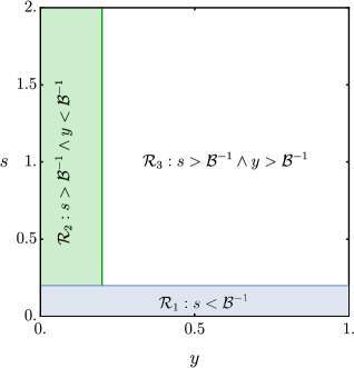
Figure 1: The three integration regions in the domain $(y,s)\in[0,1]\times[0,\infty]$, as described in the text.

Notice that the presence of the counter-term makes the integrand to identically vanish in the limit $s\rightarrow 0$. Similarly, in the limit $y\rightarrow 0$, the integrand is finite. Therefore, for large magnetic fields, $\mathcal{B}\gg 1$, it is convenient to split the integration domain $(y,s)\in[0,1]\times[0,\infty]$ into three separate regions $(\mathcal{R}_{1},\mathcal{R}_{2},\mathcal{R}_{3})$, as depicted in Fig. 1, as follows

$$\int_{0}^{1}dy\int_{0}^{\infty}ds$$

$$= \underbrace{\int_{0}^{1}dy\int_{0}^{\mathcal{B}^{-1}}}_{\mathcal{R}_{1}}ds+\underbrace{\int_{0}^{\mathcal{B}^{-1}}dy\int_{\mathcal{B}^{-1}}^{\infty}}_{\mathcal{R}_{2}}ds+\underbrace{\int_{\mathcal{B}^{-1}}^{1}dy\int_{\mathcal{B}^{-1}}^{\infty}}_{\mathcal{R}_{3}}ds,$$

such that we write the mass shift components as

$$\delta m_{B}^{(\pm)} = \left.\delta m_{B}^{(\pm)}\right|_{\mathcal{R}_{1}}+\left.\delta m_{B}^{(\pm)}\right|_{\mathcal{R}_{2}}+\left.\delta m_{B}^{(\pm)}\right|_{\mathcal{R}_{3}}.$$ (42)

The integrand in the first term, where $\mathcal{B}s<1$, is bounded from above, and its singularity as $s\rightarrow 0$ is removed by the counter-term. Moreover (see Appendix C for details), its contribution is

$$\left.\delta m_{B}^{(\pm)}\right|_{\mathcal{R}_{1}} = \frac{2me^{2}}{(4\pi)^{2}}\left(-\frac{157}{2016}+\frac{2041}{56700}i\mathcal{B}^{-1}\right.$$ (43)

$$\mp \left.\left[\frac{91}{540}-\frac{257}{10080}i\mathcal{B}^{-1}\right]\right)+O(\mathcal{B}^{-2}).$$

Similarly, as shown in Appendix C, the contribution arising from the second region is (for $\mathcal{B}\gg 1$)

$$\left.\delta m_{B}^{(\pm)}\right|_{\mathcal{R}_{2}} \sim\frac{2me^{2}}{(4\pi)^{2}}\left\{-1-2\mathcal{B}^{-1}\ln(\mathcal{B})+\mathcal{B}^{-1}\left(2\gamma\right.\right.$$

$$\left.\left.-2\ln\left[|1-e^{2i}|\right]+i\left(\pi\pm\frac{1}{2}\right)\right)\right\}+O(\mathcal{B}^{-2}).$$

The contribution of both of these subleading kinematic regions becomes finite and strictly real as $\mathcal{B}\rightarrow\infty$.

Finally, for the remaining, and hence dominant, kinematic region, characterized by the condition $\mathcal{B}s\gg 1$, since $|\sin(\mathcal{B}s(1-y))|\leq 1$, we have the inequality

$$\left|\frac{\sin(\mathcal{B}s(1-y))}{\mathcal{B}s}\right|\leq\frac{1}{\mathcal{B}s}\ll 1$$ (45)

Under this assumption, the asymptotic expression for the mass shift components in Eq. (37) is

$$\left.\delta m_{B}^{(\pm)}\right|_{\mathcal{R}_{3}} = \frac{2me^{2}}{(4\pi)^{2}}\int_{\mathcal{B}^{-1}}^{1}dy\int_{\mathcal{B}^{-1}}^{\infty}\frac{ds}{s}$$ (46)

$$\times e^{is\left(-(1-y)^{2}+i\epsilon\right)}\left[\frac{(2-y)(1-y)}{y}\right.$$

$$\left.\mp\tan(\mathcal{B}s(1-y))\right].$$

We notice the presence of the $\tan(\mathcal{B}s(1-y))$ function in the integrand of Eq. (46), which is continuous when defined in the open interval $(-\frac{\pi}{2},\frac{\pi}{2})$, and extends itself periodically along the real axis, namely, $\tan(x+n\pi)=\tan(x)$, possessing infinitely many poles at every odd multiple of $\pi/2$, i.e. for $x\rightarrow\pm\frac{(2n-1)\pi}{2}$, $\tan(x)\to\pm\infty$. Therefore, the integral in Eq. (46) must be interpreted as a principal value and hence, in the sense of distributions, we can use the periodic series (see Appendix D for details)

$$\tan( \!\!\mathcal{B}\!\! s(1-y))=2\sum_{n=1}^{\infty}(-1)^{n-1}\sin(2\mathcal{B}s(1-y))$$ (47)

$$= i\sum_{n=1}^{\infty}(-1)^{n}\left(e^{2in\mathcal{B}s(1-y)}-e^{-2in\mathcal{B}s(1-y)}\right).$$

Substituting Eq. (47) into Eq. (46), and using the exact definitions (as $\epsilon\rightarrow 0^{+}$),

$$\int_{\mathcal{B}^{-1}}^{\infty}\frac{ds}{s}e^{is\left(-(1-y)^{2}+i\epsilon\right)} = \Gamma\left(0,i\frac{(1-y)^{2}}{\mathcal{B}}\right),$$ (48)

$$\int_{1/\mathcal{B}}^{\infty}\frac{ds}{s}e^{is\left(-(1-y)(1-y\pm 2n\mathcal{B})+i\epsilon\right)}=$$

$$\Gamma\left(0,i\frac{(1-y)(1-y\pm 2n\mathcal{B})}{\mathcal{B}}\right),$$ (49)

we obtain that the magnetic mass shift components are given by

$$\left.\delta m_{B}^{(\pm)}\right|_{\mathcal{R}_{3}}=\frac{2me^{2}}{(4\pi)^{2}}\int_{\mathcal{B}^{-1}}^{1}dy\Bigg{[}\frac{(2-y)(1-y)}{y}$$ (50)

$$\times \Gamma\left(0,i\frac{(1-y)^{2}}{\mathcal{B}}\right)$$

$$\mp i\sum_{n=1}^{\infty}(-1)^{n}\left\{\Gamma\left(0,i\frac{(1-y)(1-y-2n\mathcal{B})}{\mathcal{B}}\right)\right.$$

$$\left.-\Gamma\left(0,i\frac{(1-y)(1-y+2n\mathcal{B})}{\mathcal{B}}\right)\right\}\Bigg{]}.$$

We notice that the incomplete Gamma function $\Gamma(0,z)$ satisfies the following identity

$$\Gamma(0,iz)=-\gamma-\ln(iz)-\sum_{k=1}^{\infty}\frac{(-iz)^{k}}{k\,(k!)}.$$ (51)

Therefore, for large $\mathcal{B}\gg 1$ we have the following asymptotics

$$\!\!\!\!\!\!\!\!\Gamma\left(0,i\frac{(1-y)^{2}}{\mathcal{B}}\right)\!\!=\!\!-\gamma-\ln\left(i\frac{(1-y)^{2}}{\mathcal{B}}\right)\!+O\left(\mathcal{B}^{-1}\right)\!,$$ (52)

thus leading to a double logarithmic dependence of the mass shift operator $\delta m_{B}\sim\left(\ln(\mathcal{B})\right)^{2}$ for $\mathcal{B}\gg 1$. More precisely, as shown in Appendix D, the integrals involved in Eq. (50) display the following asymptotic behavior (for $\mathcal{B}\gg 1$),

$$\int_{\mathcal{B}^{-1}}^{1}\frac{dy}{y}(1-y)(2-y)\Gamma[0,i\mathcal{B}^{-1}(1-y)^{2}]$$ (53)

$$= 2\left[\ln(\mathcal{B})\right]^{2}-\left(2\gamma+\frac{5}{2}+i\pi\right)\ln(\mathcal{B})+O(\mathcal{B}^{0}),$$

and the infinite sum over Landau levels in Eq. (50), as shown in Appendix E, is given by

$$\pm i\sum_{n=1}^{\infty}\int_{\mathcal{B}^{-1}}^{1}dy\left\{\Gamma[0,i\mathcal{B}^{-1}(1-y)(1-y-2n\mathcal{B})]\right.$$

$$\left.-\Gamma[0,i\mathcal{B}^{-1}(1-y)(1-y+2n\mathcal{B})]\right\}$$

$$=\mp 0.421794\left(1-\mathcal{B}^{-1}\right)\mp\ln(2)\pm i\left(1-\mathcal{B}^{-1}\right)\frac{\ln(2)}{2}$$

$$+O(\mathcal{B}^{-2}).$$ (54)

Therefore, the dominant contribution to the magnetic mass shift components is, after Eq. (50) (for $\mathcal{B}\gg 1$)

$$\left.\delta m_{B}^{(\pm)}\right|_{\mathcal{R}_{3}} = \frac{2me^{2}}{(4\pi)^{2}}\Bigg{\{}2\left[\ln(\mathcal{B})\right]^{2}-\left[2\gamma+\frac{5}{2}+i\pi\right]\ln(\mathcal{B})\Bigg{\}}$$ (55)

$$+O(\mathcal{B}^{0}).$$

Note that the above result is the same when only the LLL is taken into account. Moreover, given that Eq. (55) is independent of the sign of the projection, we rename it as $\left.\delta m_{B}\right|_{\mathcal{R}_{3}}$.

​​

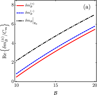
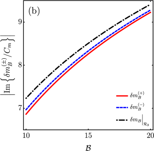
Figure 2: (a) Real and (b) imaginary parts for both projections $(\pm)$ of the mass-shift given in Eq. (42), compared with the dominant $\left.\delta m_{B}\right|_{\mathcal{R}_{3}}$ contribution.

​​

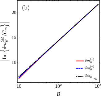
Figure 3: (a) Real and (b) imaginary parts for both projections $(\pm)$ of the mass-shift given in Eq. (42), compared with the dominant $\left.\delta m_{B}\right|_{\mathcal{R}_{3}}$ contribution.

V Analysis of the results

In order to interpret the results obtained, let us write the inverse propagator in momentum space and at finite magnetic field in the form

$$\left.[-iS_{F}(p)\right]^{-1} = \not{p}-m-\Sigma(p,B)$$

$$= \left(\hat{O}^{(+)}+\hat{O}^{(-)}\right)\left(\not{p}-m\right)-\hat{O}^{(+)}\Sigma^{(+)}(p,B)$$

$$- \hat{O}^{(-)}\Sigma^{(-)}(p,B)$$

$$= \hat{O}^{(+)}\left[-i\Delta_{F}^{(+)}(p)\right]^{-1}+\hat{O}^{(-)}\left[-i\Delta_{F}^{(-)}(p)\right]^{-1}$$

where the Feynman propagators for each spin projection $(\pm)$ parallel to the magnetic field direction are thus given by

$$\Delta_{F}^{(\pm)}(p)=\frac{i}{\not{p}-m-\Sigma^{(\pm)}(p,B)+i\epsilon}.$$ (57)

As obtained after the explicit calculations in the previous section, the pole in each of these propagators contains an imaginary part, whose magnitude scales as $\text{Im}\Sigma^{(\pm)}(m,B)\sim-\ln(\mathcal{B})$, while the real part scales as $\text{Re}\Sigma^{(\pm)}(m,B)\sim\left[\ln(\mathcal{B})\right]^{2}$, and hence the latter becomes dominant at large magnetic fields, $\mathcal{B}\gg 1$. Therefore, the physical mass is determined by the real part,

$$m_{B}^{(\pm)}=m+\text{Re}\Sigma^{(\pm)}(m,B),$$ (58)

while the imaginary part determines an spectral width, since near the pole

$$\!\!\!\!\!\!\!\!\!\Delta_{F}^{(\pm)}(p) \sim \frac{i}{\not{p}-m_{B}^{(\pm)}-i\text{Im}\Sigma^{(\pm)}(m,B)+i\epsilon}$$ (59)

$$\sim i\frac{\not{p}+m_{B}^{(\pm)}+i\text{Im}\Sigma^{(\pm)}(m,B)}{p^{2}-\left(m_{B}^{(\pm)}\right)^{2}-2im_{B}^{(\pm)}\text{Im}\Sigma^{(\pm)}(m,B)}.$$

Figures 2 and 3 show the behavior of the real and imaginary parts for both projections $(\pm)$ of the mass-shift given in Eq. (42), compared with the dominant $\left.\delta m_{B}\right|_{\mathcal{R}_{3}}$. All the contributions are normalized to the quantity $C_{m}=2me^{2}/(4\pi)^{2}$. Figure 2 shows the case for a moderate range of the field strength in units of the fermion mass whereas Fig. 3 is for the case of a larger range of field strengths. It is important to mention, that our approximation is valid in the region where $\ln\mathcal{B}\geq 1$, therefore, the results have $\mathcal{B}\sim 10$ as a lower limit. Notice that as the field strength increases, both the real and the imaginary parts are better described by the dominant contribution which in turn comes from the LLL or $\left.\delta m_{B}\right|_{\mathcal{R}_{3}}$.

The appearance of an imaginary part is an interesting and expected feature, which has a direct physical picture: An electron not yet affected by the magnetic field (corresponding to the external leg in the self-energy diagram) enters a region where the magnetic field forces it to occupy a Landau level and thus (in classical terms), an orbit around the field lines. The emission of photons comes from the fact that the fermion need to preserve its energy and momentum (a syncroton-like process). At lowest order, this is represented by the emission of one photon, but as we shall see, when the Landau levels are close to each other, the process is better represented by a distribution of Landau levels that can possibly be occupied and thus the need of the spectral function representation. In that spirit, note that the real and imaginary parts combined define a Breit-Wigner resonance $\Gamma^{(\pm)}=-2\text{Im}\Sigma^{(\pm)}(m,B)$, whose relative width

$$\frac{\Gamma^{(\pm)}}{m_{B}^{(\pm)}} = -\frac{2\text{Im}\Sigma^{(\pm)}(m,B)}{m_{B}^{(\pm)}}\sim\frac{\ln(\mathcal{B})}{\left[\ln(\mathcal{B})\right]^{2}}\sim\left[\ln(\mathcal{B})\right]^{-1}$$ (60)

decreases to zero at a rate $\left[\ln(\mathcal{B})\right]^{-1}$ as the magnetic field grows large ($\mathcal{B}\rightarrow\infty$). This effect can be highlighted analyzing the spectral density, which is, as usual, calculated from the imaginary part of the scalar denominator in the Feynman propagator. For a well defined single-particle state with mass $m_{B}^{(\pm)}$, we would have (as $\epsilon\rightarrow 0^{+}$)

$$\widetilde{\rho}(p^{2}) = -\frac{1}{\pi}\text{Im}\left(\frac{1}{p^{2}-\left(m_{B}^{(\pm)}\right)^{2}+i\epsilon}\right)$$ (61)

$$= \frac{\epsilon/\pi}{\left(p^{2}-\left(m_{B}^{(\pm)}\right)^{2}\right)^{2}+\epsilon^{2}}$$

$$\,\,\,\delta\left[p^{2}-\left(m_{B}^{(\pm)}\right)^{2}\right].$$

In the present case, however, due to the presence of a finite imaginary part in the pole, a similar calculation leads to a spectral density of the form

$$\widetilde{\rho}(p^{2}) = -\frac{1}{\pi}\text{Im}\left(\frac{1}{p^{2}-\left(m_{B}^{(\pm)}\right)^{2}+im_{B}^{(\pm)}\Gamma^{(\pm)}+i\epsilon}\right)$$

$$= \frac{\epsilon/\pi+m_{B}^{(\pm)}\Gamma^{(\pm)}/\pi}{\left(p^{2}-\left(m_{B}^{(\pm)}\right)^{2}\right)^{2}+\left(m_{B}^{(\pm)}\Gamma^{(\pm)}+\epsilon\right)^{2}}$$

$$\sim \frac{m_{B}^{(\pm)}\Gamma^{(\pm)}/\pi}{\left(p^{2}-\left(m_{B}^{(\pm)}\right)^{2}\right)^{2}+\left[m_{B}^{(\pm)}\Gamma^{(\pm)}\right]^{2}},$$

that clearly shows a smeared, roughly Lorentzian distribution, representing a quasi-continuum of unstable energy states. While the dominant contribution at very large values of the magnetic field can be easily traced back to the LLL, the smearing is related to the probability to populate the higher Landau levels, with a relative width $\Gamma^{(\pm)}/m_{B}^{(\pm)}\sim\left[\ln(\mathcal{B})\right]^{-1}$ that decays to zero as $\mathcal{B}\rightarrow\infty$, and hence in this limit all the spectral weight is concentrated on the stable LLL.

​​

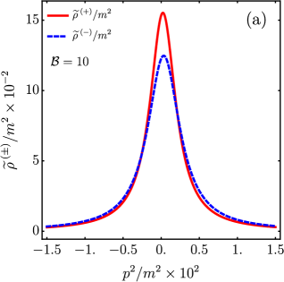
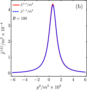
Figure 4: Spectral density from Eq. (V) for (a) $\mathcal{B}=10$ and (b) $\mathcal{B}=100$ as a function of the momentum squared. The solid line represents the contribution of $\delta m_{B}^{(+)}$ whereas the dashed line is the contribution of $\delta m_{B}^{(-)}$.

Figure 4 shows the spectral densities as functions of the momentum squared scaled by the fermion mass squared, for two values of the magnetic field $\mathcal{B}=10^{2}$ (a) and $\mathcal{B}=10^{3}$ (b). Notice that as the field strength increases, the peaks for both modes approach each other and at the same time, the Lorentzian distribution narrows.

VI Conclusions

In summary, we have studied the fermion self-energy in QED in the presence of a magnetic field. After carrying out the renormalization procedure we have shown that in the large field limit, when accounting for sub-leading contributions associated to Landau levels other than the LLL, the mass function develops also an imaginary part. From this imaginary part it is possible to define a spectral density describing the spread of the mass function in momentum which is centered at the magnetic-field modified mass. The width of this distribution becomes small as the field intensity increases in such a way that for asymptotic values of the field, when the separation between Landau levels becomes also large, the mass function describes a stable particle occupying only the LLL. For large but finite values of the magnetic field, the spectral density represents the finite probability for the fermion to occupy Landau levels other than the LLL.

The present calculation has potential applications. Recent works consider dilepton production from a single photon in a strong magnetic field, giving rise to vacuum dichroism, i.e., the spectrum becomes anisotropic with respect to the magnetic field direction, depending also on the photon polarization. Hattori et al. (2021). There, the usual QED vertex is considered when the outgoing fermions are dressed by corrections due to the external magnetic field. Nevertheless, self-energy correction for these outgoing fermions is not taken into account, which would soft the spiky structure of the spectrum through the imaginary part that we report. On the other hand, in the field of condensed matter systems, the vacuum-polarization diagram plays an important role in the optical conductivity and transparency in graphene Falomir et al. (2018); Valenzuela et al. (2015). Normally, the fermion propagators are dressed by external field corrections but the inclusion of quantum self-energy corrections for the fermion propagators, as we have done in this paper, have not been considered. Certainly it would be interesting to explore the relevance of this correction for the optical transparency of graphene in the presence of an external magnetic field.

Finally, it is important to mention the range of validity of our approach, in terms of the magnetic field strength. As discussed in the main text, we focus in the region where $\ln\mathcal{B}\geq 1$ so that $\mathcal{B}\sim 10$ is a lower limit of validity, and no restrictions over the upper limit were done. However, notice that, when the real part of the magnetic field-dependent coefficient that multiplies the mass, $\eta$, that represents the dimensionless mass correction, becomes of order $\mathcal{O}(1)$, it is important to re-sum all the leading double logarithmic corrections. As it is discussed in Ref. Gusynin and Smilga (1999) when the resummation becomes singular at some value of $\eta$, this signals the breakdown of perturbation theory and the transition to the non-perturbative regime is heralded. In that regime, the coupling may also receive important magnetic field corrections which certainly deserve a thorough investigation but are outside the scope of the present work.

Appendix A Gauging away the phase factor

It is well known that in the presence of an external magnetic field, charged particle propagators can develop a phase factor $\Phi(x,x^{\prime})$. In particular, the fermion propagator $S_{f}(x,x^{\prime})$ including the phase factor, is given by

$$S_{F}(x,x^{\prime})=\Phi(x,x^{\prime})\int\frac{d^{4}p}{(2\pi)^{4}}e^{-p\cdot(x-x^{\prime})}S_{F}(p),$$ (63)

where $S_{F}(p)$ is given by Eq. (3) and the phase takes the form

$$\Phi(x,x^{\prime})=\exp\Big{\{}ie\int_{x}^{x^{\prime}}d\xi^{\mu}\left[A_{\mu}+\frac{1}{2}F_{\mu\nu}(\xi-x^{\prime})^{\nu}\right]\Big{\}}.$$

In order to perform the integral, let us take a straight line path parametrized as

$$\xi^{\mu}=x^{\prime\mu}+t(x^{\mu}-x^{\prime\mu}),\text{ for }0<t<1.$$ (65)

Therefore, the phase actor becomes

$$\Phi(x,x^{\prime})=\exp\left[ie\int_{0}^{1}A_{\mu}(x^{\mu}-x^{\prime\mu})dt\right],$$ (66)

where the anti-symmetry of $F_{\mu\nu}$ was used.

From the above, the phase can be removed by the gauge transformation

$$A_{\mu}(\xi)\to A^{\prime}_{\mu}(\xi)+\frac{\partial}{\partial\xi^{\mu}}\alpha(\xi).$$ (67)

For our case, where the magnetic field is oriented in the $z$-direction, we have

$$A_{\mu}=\frac{B}{2}(0,-x_{2},x_{1},0).$$ (68a)

Therefore, choosing

$$\alpha(\xi)=\frac{B}{2}(x_{2}^{\prime}\xi^{1}-x_{1}^{\prime}\xi_{2}^{\prime}),$$ (68b)

we obtain

$$A_{\mu}^{\prime}=\frac{B}{2}(0,x_{2}-x_{2}^{\prime},x_{1}-x_{1}^{\prime},0),$$ (69)

which implies that

$$A_{\mu}^{\prime}(x^{\mu}-x^{\prime\mu})=0,$$ (70)

and thus the phase can be safely removed.

Appendix B Dirac algebra

Here we list the properties of products of Dirac matrices that appear in the calculation of the fermion self-energy in the presence of a magnetic field:

$$\gamma_{\mu}\gamma^{\mu} = 4$$ (71)

$$\gamma_{\mu}\gamma^{1}\gamma^{2}\gamma^{\mu} = 4g^{12}=0$$ (72)

$$\gamma^{\mu}\not{k}_{\parallel}\gamma_{\mu} = k_{\parallel,\nu}\gamma^{\mu}\gamma^{\nu}\gamma_{\mu}=-2k_{\parallel,\nu}\gamma^{\nu}=-2\not{k}_{\parallel}$$ (73)

$$\gamma^{\mu}\not{k}_{\perp}\gamma_{\mu} = -2\not{k}_{\perp}$$ (74)

$$\gamma_{\mu}\gamma^{1}\gamma^{2}\not{k}_{\parallel}\gamma^{\mu} = k_{\parallel,\nu}\gamma^{\mu}\gamma^{1}\gamma^{2}\gamma^{\nu}\gamma_{\mu}=-2\not{k}_{\parallel}\gamma^{1}\gamma^{2}$$ (75)

Appendix C Subdominant integration region

As presented in the main text, the magnetic mass shift components are given by

$$\delta m_{B}=\hat{O}^{(+)}\delta m_{B}^{(+)}+\hat{O}^{(-)}\delta m_{B}^{(-)},$$ (76)

where the magnetic mass shift components are given by the integral expressions

$$\delta m_{B}^{(\pm)}=\frac{2me^{2}}{(4\pi)^{2}}$$ (77)

$$\times \int_{0}^{1}dy\int_{0}^{\infty}\frac{ds}{s}\,e^{is\left(-(1-y)^{2}+i\epsilon\right)}$$

$$\times \left[\frac{(2-y)\cos(\mathcal{B}s(1-y))}{y\cos(\mathcal{B}s(1-y))+\frac{\sin(\mathcal{B}s(1-y))}{\mathcal{B}s}}-(2-y)\right.$$

$$\left.\mp\frac{y\sin(\mathcal{B}s(1-y))}{y\cos(\mathcal{B}s(1-y))+\frac{\sin(\mathcal{B}s(1-y))}{\mathcal{B}s}}\right].$$

Moreover, as explained in the main text, we shall split the integration domain into three subregions, as follows

$$\delta m_{B}^{(\pm)} = \left.\delta m_{B}^{(\pm)}\right|_{\mathcal{R}_{1}}+\left.\delta m_{B}^{(\pm)}\right|_{\mathcal{R}_{2}}+\left.\delta m_{B}^{(\pm)}\right|_{\mathcal{R}_{3}}.$$ (78)

Let us now restrict ourselves to the kinematic region $0\leq\mathcal{B}s<1$, which corresponds to the $s$-integral domain $s\in[0,\mathcal{B}^{-1})$. Within this region, we can Taylor expand the expressions in the square bracket as a power series in $\mathcal{B}s<1$, to obtain

$$\frac{(2-y)\cos(\mathcal{B}s(1-y))}{y\cos(\mathcal{B}s(1-y))+\frac{\sin(\mathcal{B}s(1-y))}{\mathcal{B}s}}-(2-y)$$ (79)

$$= -\frac{(2-y)(1-y)^{3}}{3}\left(\mathcal{B}s\right)^{3}$$

$$- \frac{(2-y)(1+5y)(1-y)^{5}}{45}\left(\mathcal{B}s\right)^{4}+O\left(\mathcal{B}s\right)^{5},$$

and similarly

$$\frac{y\sin(\mathcal{B}s(1-y))}{y\cos(\mathcal{B}s(1-y))+\frac{\sin(\mathcal{B}s(1-y))}{\mathcal{B}s}}=y(1-y)\left(\mathcal{B}s\right)$$ (80)

$$+ \frac{y^{2}(1-y)^{3}}{3}\left(\mathcal{B}s\right)^{3}+O\left(\mathcal{B}s\right)^{5}.$$

Integrating the first group of terms, we obtain

$$\int_{0}^{1}dy\int_{0}^{\mathcal{B}^{-1}}\frac{ds}{s}e^{is\left(-(1-y)^{2}+i\epsilon\right)}$$

$$\times \left[\frac{(2-y)\cos(\mathcal{B}s(1-y))}{y\cos(\mathcal{B}s(1-y))+\frac{\sin(\mathcal{B}s(1-y))}{\mathcal{B}s}}-(2-y)\right]$$

$$\sim \frac{i\mathcal{B}^{2}}{360}\left[2\left(30i\left(2\mathcal{B}^{2}+1\right)\text{Ei}\left(-\frac{i}{\mathcal{B}}\right)-14ie^{-\frac{i}{\mathcal{B}}}\mathcal{B}^{2}\right.\right.$$

$$+ \left.\left.14i\mathcal{B}^{2}-30\pi\mathcal{B}^{2}-60i\gamma\mathcal{B}^{2}+30i\left(2\mathcal{B}^{2}+1\right)\log(\mathcal{B})\right.\right.$$

$$\left.\left.-7e^{-\frac{i}{\mathcal{B}}}\mathcal{B}-24\mathcal{B}-64ie^{-\frac{i}{\mathcal{B}}}-30i-15\pi-30i\gamma\right)\right.$$

$$+ \left.15\sqrt[4]{-1}\sqrt{\pi}(\mathcal{B}-6i)\sqrt{\mathcal{B}}\,\text{Erfi}\left(\frac{(-1)^{3/4}}{\sqrt{\mathcal{B}}}\right)\right]$$

$$= -\frac{157}{2016}+\frac{2041}{56700}i\mathcal{B}^{-1}+\frac{14749}{1425600}\mathcal{B}^{-2}+O(\mathcal{B}^{-3}),$$

and similarly, for the second term

$$\int_{0}^{1}dy\int_{0}^{\mathcal{B}^{-1}}\frac{ds}{s}e^{is\left(-(1-y)^{2}+i\epsilon\right)}$$ (82)

$$\times \left[\frac{y\sin(\mathcal{B}s(1-y))}{y\cos(\mathcal{B}s(1-y))+\frac{\sin(\mathcal{B}s(1-y))}{\mathcal{B}s}}\right]$$

$$\sim \frac{1}{12}i\mathcal{B}\left[\left(6-4\mathcal{B}^{2}\right)\text{Ei}\left(-\frac{i}{\mathcal{B}}\right)+2\left(3-2\mathcal{B}^{2}\right)\log(\mathcal{B})\right.$$

$$\left.-6\sqrt[4]{-1}\sqrt{\pi}\sqrt{\mathcal{B}}(\mathcal{B}-i)\text{Erf}\left(\frac{\sqrt[4]{-1}}{\sqrt{\mathcal{B}}}\right)+2\mathcal{B}\left(\mathcal{B}\left(-3e^{-\frac{i}{\mathcal{B}}}\right.\right.\right.$$

$$\left.\left.\left.+3+2\gamma-i\pi\right)+i\right)+12-6\gamma+3i\pi\right]$$

$$=\frac{91}{540}-\frac{257}{10080}i\mathcal{B}^{-1}-\frac{307}{75600}\mathcal{B}^{-2}+O(\mathcal{B}^{-3}).$$

Combining both expressions, we obtain for the contribution of this first kinematic region

$$\left.\delta m_{B}^{(\pm)}\right|_{\mathcal{R}_{1}} = \frac{2me^{2}}{(4\pi)^{2}}\left(-\frac{157}{2016}+\frac{2041}{56700}i\mathcal{B}^{-1}\right.$$ (83)

$$\mp \left.\left[\frac{91}{540}-\frac{257}{10080}i\mathcal{B}^{-1}\right]\right)+O(\mathcal{B}^{-2}).$$

Let us now consider the second integration region defined in the main text (see Fig. 1), corresponding to $s\in(\mathcal{B}^{-1},\infty)$ and $y\in[0,\mathcal{B}^{-1})$. The last condition means that, for large magnetic fields $\mathcal{B}\gg 1$ the integration variable $y\ll 1$ within this interval. Therefore, a Taylor expansion around $y=0$ yields for the first term,

$$e^{is\left(-(1-y)^{2}+i\epsilon\right)}(2-y)$$

$$\times\left[\frac{\cos(\mathcal{B}s(1-y))}{y\cos(\mathcal{B}s(1-y))+\frac{\sin(\mathcal{B}s(1-y))}{\mathcal{B}s}}-1\right]=e^{-is(1-i\epsilon)}\left(\mathcal{B}s-\right.$$

$$\left.\cot(\mathcal{B}s)\right)+ye^{-is(1-i\epsilon)}\left(1+2(\mathcal{B}s)^{2}-4is-\mathcal{B}s\cot(\mathcal{B}s)\right.$$

$$\left.+4i\mathcal{B}s^{2}\cot(\mathcal{B}s)\right)+O(y^{2}),$$ (84)

and similarly for the second term

$$e^{is\left(-(1-y)^{2}+i\epsilon\right)}\frac{y\sin(\mathcal{B}s(1-y))}{y\cos(\mathcal{B}s(1-y))+\frac{\sin(\mathcal{B}s(1-y))}{\mathcal{B}s}}$$ (85)

$$= ye^{-is(1-i\epsilon)}\mathcal{B}s+O(y^{2}).$$

Integrating these expressions in their corresponding kinematic region, we obtain for Eq. (84)

$$\int_{0}^{\mathcal{B}^{-1}}dy\int_{\mathcal{B}^{-1}}^{\infty}\frac{ds}{s}e^{is\left(-(1-y)^{2}+i\epsilon\right)}(2-y)$$

$$\times\left[\frac{\cos(\mathcal{B}s(1-y))}{y\cos(\mathcal{B}s(1-y))+\frac{\sin(\mathcal{B}s(1-y))}{\mathcal{B}s}}-1\right]$$

$$\sim\int_{\mathcal{B}^{-1}}^{\infty}dse^{-is\left(1-i\epsilon\right)}\left[s-2i\mathcal{B}^{-2}-2\frac{\mathcal{B}^{-1}}{s}+\frac{\mathcal{B}^{-2}}{2s}\right.$$

$$\left.+\left(2-\frac{\mathcal{B}^{-1}}{2}+2i\mathcal{B}^{-1}s\right)\cot(\mathcal{B}s)\right]$$

$$=\left(\frac{1}{2}\mathcal{B}^{-2}-2\mathcal{B}^{-1}\right)\Gamma[0,i\mathcal{B}^{-1}]-e^{-i\mathcal{B}^{-1}}\left(1+i\mathcal{B}^{-1}+2\mathcal{B}^{-2}\right)$$

$$+\left(2-\frac{\mathcal{B}^{-1}}{2}\right)\left[\frac{e^{i\left(2-\mathcal{B}^{-1}\right)}}{2\mathcal{B}-1}{}_{2}F_{1}\left(1,1-\frac{1}{2\mathcal{B}};2-\frac{1}{2\mathcal{B}};e^{2i}\right)\right.$$

$$\left.+\frac{e^{i\left(-2-\mathcal{B}^{-1}\right)}}{2\mathcal{B}+1}{}_{2}F_{1}\left(1,1+\frac{1}{2\mathcal{B}};2+\frac{1}{2\mathcal{B}};e^{-2i}\right)\right]$$

$$+2\frac{ie^{i\left(2-\mathcal{B}^{-1}\right)}}{\mathcal{B}^{2}\left(2\mathcal{B}-1\right)}{}_{2}F_{1}\left(1,1-\frac{1}{2\mathcal{B}};2-\frac{1}{2\mathcal{B}};e^{2i}\right)$$

$$+2\frac{ie^{i\left(-2-\mathcal{B}^{-1}\right)}}{\mathcal{B}^{2}\left(2\mathcal{B}+1\right)}{}_{2}F_{1}\left(1,1+\frac{1}{2\mathcal{B}};2+\frac{1}{2\mathcal{B}};e^{-2i}\right)$$

$$+\frac{1}{2\mathcal{B}^{3}}\left\{e^{-i\left(\frac{1}{\mathcal{B}}+2\right)}\Phi\left(e^{-2i},2,1+\frac{1}{2\mathcal{B}}\right)\right.$$

$$-\left.e^{i\left(-\frac{1}{\mathcal{B}}+2\right)}\Phi\left(e^{-2i},2,1-\frac{1}{2\mathcal{B}}\right)\right\}$$

$$\sim-1-2\mathcal{B}^{-1}\ln(\mathcal{B})+\mathcal{B}^{-1}\left(2\gamma-2\ln\left[|1-e^{2i}|\right]+i\pi\right)$$

$$+O(\mathcal{B}^{-2})$$ (86)

and for Eq. (85)

$$\int_{0}^{\mathcal{B}^{-1}}dy\int_{\mathcal{B}^{-1}}^{\infty}\frac{ds}{s}e^{is\left(-(1-y)^{2}+i\epsilon\right)}$$

$$\times\frac{y\sin(\mathcal{B}s(1-y))}{y\cos(\mathcal{B}s(1-y))+\frac{\sin(\mathcal{B}s(1-y))}{\mathcal{B}s}}$$

$$\sim-\frac{i}{2\mathcal{B}}e^{-i\mathcal{B}^{-1}}$$ (87)

$$=-\frac{i}{2}\mathcal{B}^{-1}+O(\mathcal{B}^{-2})$$

In these expressions, we have used the periodic series expansion (see Appendix D)

$$\cot(\mathcal{B}s)=-i\sum_{n=1}^{\infty}\left(e^{2in\mathcal{B}s}-e^{-2in\mathcal{B}s}\right)$$ (88)

to obtain the analytical integrals

$$\int_{\mathcal{B}^{-1}}^{\infty}dse^{-is\left(1-i\epsilon\right)}\cot(\mathcal{B}s)=\sum_{n=1}^{\infty}\left[\frac{e^{-i\left(1-2n\mathcal{B}\right)\mathcal{B}^{-1}}}{-1+2n\mathcal{B}}\right.$$

$$\left.+\frac{e^{-i\left(1+2n\mathcal{B}\right)\mathcal{B}^{-1}}}{1+2n\mathcal{B}}\right]$$

$$=\frac{e^{i\left(2-\mathcal{B}^{-1}\right)}}{2\mathcal{B}-1}{}_{2}F_{1}\left(1,1-\frac{1}{2\mathcal{B}};2-\frac{1}{2\mathcal{B}};e^{2i}\right)$$

$$+\frac{e^{i\left(-2-\mathcal{B}^{-1}\right)}}{2\mathcal{B}+1}{}_{2}F_{1}\left(1,1+\frac{1}{2\mathcal{B}};2+\frac{1}{2\mathcal{B}};e^{-2i}\right)$$ (89)

and

$$\int_{\mathcal{B}^{-1}}^{\infty}dse^{-is\left(1-i\epsilon\right)}s\cot(\mathcal{B}s)=i\sum_{n=1}^{\infty}\left[\frac{e^{-i\left(1-2n\mathcal{B}\right)}}{\left(1-2n\mathcal{B}\right)^{2}}\right.$$

$$\left.-\frac{e^{-i\left(1+2n\mathcal{B}\right)}}{\left(1+2n\mathcal{B}\right)^{2}}\right]-\mathcal{B}^{-1}\sum_{n=1}^{\infty}\left[\frac{e^{-i\left(1-2n\mathcal{B}\right)}}{1-2n\mathcal{B}}\right.$$

$$\left.-\frac{e^{-i\left(1+2n\mathcal{B}\right)}}{1+2n\mathcal{B}}\right]$$

$$=\frac{e^{i\left(2-\mathcal{B}^{-1}\right)}}{\mathcal{B}\left(2\mathcal{B}-1\right)}{}_{2}F_{1}\left(1,1-\frac{1}{2\mathcal{B}};2-\frac{1}{2\mathcal{B}};e^{2i}\right)$$

$$+\frac{e^{i\left(-2-\mathcal{B}^{-1}\right)}}{\mathcal{B}\left(2\mathcal{B}+1\right)}{}_{2}F_{1}\left(1,1+\frac{1}{2\mathcal{B}};2+\frac{1}{2\mathcal{B}};e^{-2i}\right)$$

$$-\frac{i}{4\mathcal{B}^{2}}\left\{e^{-i\left(\frac{1}{\mathcal{B}}+2\right)}\Phi\left(e^{-2i},2,1+\frac{1}{2\mathcal{B}}\right)\right.$$

$$-\left.e^{i\left(-\frac{1}{\mathcal{B}}+2\right)}\Phi\left(e^{-2i},2,1-\frac{1}{2\mathcal{B}}\right)\right\}$$ (90)

where ${}_{2}F_{1}(a,b;c;z)$ is the Hypergeometric function, while $\Phi(z,s,a)$ is the Hurwitz-Lerch transcendent function, along with the exact infinite series expressions

$$\sum_{n=1}^{\infty}\frac{e^{-i\left(1+2n\mathcal{B}\right)/\mathcal{B}}}{1+2n\mathcal{B}} = \frac{e^{-i\left(2+\mathcal{B}^{-1}\right)}}{1+2\mathcal{B}}$$

$$\times{}_{2}F_{1}\left(1,1+\frac{1}{2\mathcal{B}};2+\frac{1}{2\mathcal{B}};e^{-2i}\right)$$

$$\sum_{n=1}^{\infty}\frac{e^{-i\left(1+2n\mathcal{B}\right)/\mathcal{B}}}{\left(1+2n\mathcal{B}\right)^{2}} = \frac{e^{-i\left(2+\mathcal{B}^{-1}\right)}}{4\mathcal{B}^{2}}\Phi\left(e^{-2i},2,1+\frac{1}{2\mathcal{B}}\right)$$

Combining these expressions, we obtain for the mass shift contribution in this second subdominant kinematic region

$$\left.\delta m_{B}^{(\pm)}\right|_{\mathcal{R}_{2}} \sim\frac{2me^{2}}{(4\pi)^{2}}\left\{-1-2\mathcal{B}^{-1}\ln(\mathcal{B})+\mathcal{B}^{-1}\left(2\gamma\right.\right.$$

$$\left.\left.-2\ln\left[|1-e^{2i}|\right]+i\left(\pi\pm\frac{1}{2}\right)\right)\right\}+O(\mathcal{B}^{-2}).$$

Appendix D A periodic series expansion for the functions $tan(x)$ and $cot(x)$

The function $\tan(z)$ possesses infinitely many isolated poles over the real axis, at every odd multiple of $\pi/2$, i.e. at $z_{j}=(2j-1)\pi/2$, $j\in\mathbb{Z}$, and it is periodic with fundamental period $\pi$, $\tan(z+\pi)=\tan(z)$. Therefore, in the domain of complex functions, it only admits a Laurent series representations defined inside concentric open discs of the form $|z|<\pi/2$, $\pi/2<|z|<3\pi/2$, etc. It is therefore possible to obtain an explicit representation within the open real interval $\text{Re}z=x\in(-\pi/2,\pi/2)$, that extends periodically to all the open intervals of the form $(-(2j-1)\pi/2,(2j-1)\pi/2)$. For this purpose, let us first consider the general definition in the complex plane

$$\tan(z) = \frac{\sin(z)}{\cos(z)}=-i\frac{e^{iz}-e^{-iz}}{e^{iz}+e^{-iz}}$$ (93)

$$= -\frac{d}{dz}\log\left(e^{iz}+e^{-iz}\right)$$

The complex $\log(z)=\ln|z|+i\arg(z)$ is an analytic function, and hence it possesses a Taylor series with convergence radius $|z|\leq 1$

$$\log(1+z)=\sum_{n=1}^{\infty}\frac{(-1)^{n-1}}{n}z^{n},\,\,\,|z|\leq 1.$$ (94)

Therefore, using Eq. (94), we obtain the convergent series for $|e^{-2iz}|\leq 1$ (or equivalently for $\text{Im}z\leq 0$)

$$\log\left(e^{iz}+e^{-iz}\right) = \log\left(e^{iz}\left(1+e^{-2iz}\right)\right)$$ (95)

$$= iz+\log\left(1+e^{-2iz}\right)$$

$$= iz+\sum_{n=1}^{\infty}\frac{(-1)^{n-1}}{n}e^{-2inz}.$$

Choosing $z=x\in\mathbb{R}$ ($\text{Im}z=0$) in the series (95), inserting into Eq. (93), and futher taking the real part, we obtain the following periodic series representation for the real tangent function

$$\tan(x) = 2\sum_{n=1}^{\infty}(-1)^{n-1}\sin(2nx)$$ (96)

$$= i\sum_{n=1}^{\infty}(-1)^{n}\left(e^{2inx}-e^{-2inx}\right).$$

This constitutes a generalized Fourier series representation in the open interval $(-\pi/2,\pi/2)$, that also provides a periodic extension $\tan(x+\pi)=\tan(x)$. It must, however, be interpreted in the distributional sense, and not as a strict point wise convergence, since the last is only guaranteed for the logarithm expansion in Eq. (95). Therefore, in the sense of distributions, for any continuous differentiable function $f(x)$ within an interval $x\in[a,b]$, such that $a>-\pi/2$ and $b<\pi/2$, we have

$$\int_{a}^{b}f(x)\tan(x)dx = -\text{Re}\left[\int_{a}^{b}f(x)\frac{d}{dx}\log(e^{ix}+e^{-ix})dx\right]$$ (97)

$$= \int_{a}^{b}\frac{df}{dx}(x)\text{Re}\log(e^{ix}+e^{-ix})dx$$

$$- \left[f(x)\log(e^{ix}+e^{-ix})\right]_{a}^{b}$$

and hence the integral of the series provides the correct result (thanks to the point wise convergence of Eq. (95)). This is illustrated in the upper panel of Fig.  5.

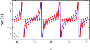
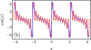
Figure 5: (a) Comparison between the periodic series Eq. (96) (truncated at 8 terms) and the function $\tan(x)$. (b) Comparison between the periodic series Eq. (100) and the function $\cot(x)$.

Following a similar analysis, we have that $\cot(z)$ is also a periodic function with fundamental period $\pi$, i.e. $\cot(z+\pi)=\cot(z)$, that possesses infinitely many poles located along the real axis at $z_{j}=j\pi$, $j\in\mathbb{Z}$. Therefore, in the domain of complex functions, it only admits a Laurent series representations defined inside concentric open discs of the form $0<|z|<\pi$, $\pi<|z|<2\pi$, etc. It is therefore possible to obtain an explicit representation within the open interval $\text{Re}z=x\in(0,\pi)$, that periodically extends to the remaining open intervals of the form $(n\pi,(n+1)\pi)$. By analogy with the previous case, we consider the definition in the complex plane of

$$\cot(z) = \frac{\cos(z)}{\sin(z)}=i\frac{e^{iz}+e^{-iz}}{e^{iz}-e^{-iz}}$$ (98)

$$= \frac{d}{dz}\log\left(e^{iz}-e^{-iz}\right)$$

Using again the convergent power series for the logarithm in Eq. (95), we have (for $\text{Im}z\leq 0$)

$$\log\left(e^{iz}-e^{-iz}\right) = iz+\sum_{n=1}^{\infty}\frac{(-1)^{n-1}}{n}\left(-e^{-2iz}\right)^{n}$$ (99)

$$= iz-\sum_{n=1}^{\infty}\frac{1}{n}e^{-2inz}.$$

As before, setting $z=x\in\mathbb{R}$ ($\text{Im}z=0$), inserting into Eq. (98) and further taking the real part, we obtain the periodic series representation for the real $cot(x)$ function

$$\cot(x) = 2\sum_{n=1}^{\infty}\sin(2nx)$$ (100)

$$= -i\sum_{n=1}^{\infty}\left(e^{2inx}-e^{-2inx}\right).$$

As in the former case, this series must be interpreted in the generalized sense of distributions, and not as point wise converging, as follows from an identical analysis as in Eq. (97). This is illustrated in the lower panel of Fig. 5.

Appendix E Integrals of the incomplete Gamma functions

Here we show the details of the calculation of the integrals of the incomplete Gamma functions. For this we use the exact series expansion

$$\Gamma(0,iz)=-\gamma-\ln(iz)-\sum_{k=1}^{\infty}\frac{(-iz)^{k}}{k(k!)},$$ (101)

and integrate the three contributions separately. Therefore, for the first integral we obtain

$$\int_{\mathcal{B}^{-1}}^{1}\frac{dy}{y}(1-y)(2-y)\Gamma[0,i\mathcal{B}^{-1}(1-y)^{2}]=2\left[\ln(\mathcal{B})\right]^{2}$$ (102)

$$+\gamma\left\{\frac{5}{2}-3\mathcal{B}^{-1}+\frac{1}{2}\mathcal{B}^{-2}-2\ln(\mathcal{B})\right\}-\frac{18+i\pi}{4}+5\mathcal{B}^{-1}$$

$$-\frac{1}{2}\mathcal{B}^{-2}-2\ln\left(i(1-\mathcal{B}^{-1})^{2}\right)\ln(\mathcal{B})$$

$$+3(1-\mathcal{B}^{-1}+\frac{1}{6}\mathcal{B}^{-2})\ln\left(\frac{i(\mathcal{B}-1)^{2}}{\mathcal{B}^{3}}\right)$$

$$+4\text{Li}_{2}\left(1-\mathcal{B}^{-1}\right)-\ln(\mathcal{B}-1)+\frac{3}{2}\ln(\mathcal{B})$$

$$-i\sum_{k=1}^{\infty}\frac{\mathcal{B}^{-k}\left(-i(1-\mathcal{B}^{-1})\right)^{k+1}}{(k+1)kk!}$$

$$\times\left\{\,{}_{2}F_{1}\left(1,2(k+1);2k+3;1-\mathcal{B}^{-1}\right)-\frac{1}{2}\right\}$$

$$= 2\left[\ln(\mathcal{B})\right]^{2}-\left(2\gamma+\frac{5}{2}+i\pi\right)\ln(\mathcal{B})+\left(3+2i\right)\mathcal{B}^{-1}\ln(\mathcal{B})$$

$$+\frac{\left(30\gamma-54+8\pi^{2}+15i\pi\right)}{12}$$

$$-\frac{\mathcal{B}^{-1}}{12}\left(48+36\gamma+i(18\pi+47)\right)+O(\mathcal{B}^{-2}).$$

Finally, for the third type of integrals, with $n=1,\ldots,\infty$, we obtain from Eq. (101)

$$\int_{\mathcal{B}^{-1}}^{1}dy\Gamma[0,i\mathcal{B}^{-1}(1-y)(1-y+2n\mathcal{B})]=-\gamma\ln(\mathcal{B})$$

$$-\int_{\mathcal{B}^{-1}}^{1}dy\ln\left[i\mathcal{B}^{-1}(1-y)(1-y+2n\mathcal{B})\right]-S(\mathcal{B},n).$$

(103)

Here, we defined the series

$$S(\mathcal{B},n) = \sum_{k=1}^{\infty}\frac{(i\mathcal{B})^{-k}}{k\,k!}\int_{\mathcal{B}^{-1}}^{1}dy\left[(1-y)(1-y+2n\mathcal{B})\right]^{k}$$

Each of the integrals can be performed analytically, to obtain

$$\int_{\mathcal{B}^{-1}}^{1} dy\left[(1-y)(1-y+2n\mathcal{B})\right]^{k}=\frac{2^{k}(\mathcal{B}-1)^{k+1}n^{k}}{\mathcal{B}(k+1)}$$ (105)

$$\times\,_{2}F_{1}\left(-k,k+1;k+2;\frac{1-\mathcal{B}}{2\mathcal{B}^{2}n}\right)$$

Here, ${}_{2}F_{1}\left(a_{1},a_{2};b_{1};z\right)$ is one of the Hypergeometric functions. Inserting this result into Eq. (103), we obtain

$$S(\mathcal{B},n) = \left(1-\mathcal{B}^{-1}\right)\sum_{k=1}^{\infty}\frac{\left(-2ni\left(1-\mathcal{B}^{-1}\right)\right)^{k}}{k(k+1)!}$$ (106)

$$\times\,_{2}F_{1}\left(-k,k+1;k+2;\frac{1-\mathcal{B}}{2\mathcal{B}^{2}n}\right).$$

Since the Hypergeometric function satisfies

$$\!\!\!\!\!\!\!{}_{2}F_{1}\left(-k,k+1;k+2;\frac{1-\mathcal{B}}{2\mathcal{B}^{2}n}\right)=1+O(\mathcal{B}^{-1}),$$ (107)

and when substituted into Eq. (106), we thus obtain the asymptotics

$$S(\mathcal{B},n) = \left(1-\mathcal{B}^{-1}\right)\sum_{k=1}^{\infty}\frac{\left(-2ni\left(1-\mathcal{B}^{-1}\right)\right)^{k}}{k(k+1)!}+O(\mathcal{B}^{-2})$$ (108)

$$= -\frac{e^{-2in}}{{2n}}\left(-ie^{2in}-2e^{2in}n+2\gamma e^{2in}n\right.$$

$$\left.+2e^{2in}n\ln(2in)+2e^{2in}n\Gamma(0,2in)+i\right)$$

$$+ \mathcal{B}^{-1}\left(\ln(2in)+\Gamma(0,2in)+\gamma\right)+O(\mathcal{B}^{-2})$$

Using this result into Eq. (103), as shown in the main text we need the combination

$$\int_{\mathcal{B}^{-1}}^{1}dy\left(\Gamma[0,i\mathcal{B}^{-1}(1-y)(1-y-2n\mathcal{B})]\right.$$

$$\left.-\Gamma[0,i\mathcal{B}^{-1}(1-y)(1-y+2n\mathcal{B})]\right)=$$

$$-\int_{\mathcal{B}^{-1}}^{1}dy\left(\ln\left[i\mathcal{B}^{-1}(1-y)(1-y-2n\mathcal{B})\right]\right.$$

$$\left.-\ln\left[i\mathcal{B}^{-1}(1-y)(1-y+2n\mathcal{B})\right]\right)+S(\mathcal{B},n)-S\left(\mathcal{B},-n\right)$$

$$=\left(1-\mathcal{B}^{-1}\right)\left(\Gamma[0,2in]-\Gamma[0,-2in]\right)$$

$$-\frac{i}{n}+\frac{i}{2n}\left(e^{2in}-e^{-2in}\right)+O(\mathcal{B}^{-2}).$$ (109)

Finally, using the Taylor expansion for the logarithm

$$\ln(1+z)=\sum_{n=1}^{\infty}\frac{(-1)^{n+1}z^{n}}{n},$$ (110)

we have the simple identities

$$\sum_{n=1}^{\infty}\frac{(-1)^{n}}{n}=-\ln(2)$$ (111a)

$$\sum_{n=1}^{\infty}\frac{(-1)^{n}}{n}\left(e^{2in}-e^{-2in}\right)$$ (111b)

$$= -\ln\left(1+e^{2i}\right)+\ln\left(1+e^{-2i}\right)$$

$$= -\ln\left(1+e^{2i}\right)+\ln\left(e^{-2i}\left(1+e^{2i}\right)\right)$$

$$= -2i,$$

along with the sum

$$\sum_{n=1}^{\infty}(-1)^{n}\left(\Gamma[0,2in]-\Gamma[0,-2in]\right)=0.421794i.$$ (112)

Therefore, we finally obtain

$$\pm i\sum_{n=1}^{\infty}\int_{\mathcal{B}^{-1}}^{1}dy\left\{\Gamma[0,i\mathcal{B}^{-1}(1-y)(1-y-2n\mathcal{B})]\right.$$ (113)

$$\left.-\Gamma[0,i\mathcal{B}^{-1}(1-y)(1-y+2n\mathcal{B})]\right\}$$

$$=\mp 0.421794\left(1-\mathcal{B}^{-1}\right)\mp\ln(2)\pm i\left(1-\mathcal{B}^{-1}\right)\frac{\ln(2)}{2}$$

$$+O(\mathcal{B}^{-2}).$$

Appendix F Connection with Ref. Tsai (1974)

In this appendix we compare our results with well-known calculations in the limit of a strong magnetic field. In particular, we demonstrate that the expressions for the counter-terms and the relevant integrals are the same as the ones presented in Ref. Tsai (1974) by Tsai. In order to do that, let us begin with Eqs. (30) and (32) which correspond to the counter-terms, namely

$$c.t._{1}=-(2-y),$$ (114)

and

$$c.t._{2}=-(\not{\rho}-1)\left[-\frac{y}{m}+2i\frac{sy(1-y)(2-y)}{m}\right],$$ (115)

so that, in terms of the canonical momentum $p^{\mu}$, the sum of counter-terms is

$$c.t._{1}+c.t._{2} = -(2-y)$$

$$+ \frac{\not{p}-m}{m}\left[\frac{y}{m}-2i\frac{sy(1-y)(2-y)}{m}\right].$$

In order to compare with Ref. Tsai (1974), it is necessary to identify our integration variables with the ones used in that work. Explicitly, the latter is given by

$$u \to 1-y$$

$$s \to m^{2}s.$$ (117)

Moreover, in Ref. Tsai (1974) the metric is

$$g^{\mu\nu}=\text{diag}(-1,1,1,1)$$ (118)

whereas we use

$$g^{\mu\nu}=\text{diag}(1,-1,-1,-1),$$ (119)

therefore, we also identify

$$\not{p}+m\to\not{p}-m.$$ (120)

Now, the counter-term in Ref. Tsai (1974) is

$$c.t.=-(1-u)-(m+\not{\Pi})\left[\frac{1-u}{m}-2imu(1-u^{2})s\right],$$

so that after applying Eqs. (117) and (120) it gives Eq. (LABEL:c1c2), with the difference that in our calculation there appears $\not{p}$ instead of $\not{\Pi}$.

For the sake of completeness, let us find the parallelism with the other expressions in the reference of interest. First, for Eq. (21) in Tsai’s work:

$$\tilde{M}(p) = \frac{\alpha}{2\pi}\int\frac{ds}{s}du\frac{e^{-is(um^{2}+\varphi)}e^{i\zeta y_{\text{T}}}}{(1-u)\cos y_{\text{T}}+u(\sin y_{\text{T}})/y_{\text{T}}}$$ (122)

$$\times \left[1+e^{-2i\zeta y_{\text{T}}}+(1-u)e^{-2i\zeta y_{\text{T}}}\frac{\not{p}_{\parallel}}{m}\right.$$

$$+ \left.\frac{(1-u)\not{p}_{\perp}/m}{(1-u)\cos y_{\text{T}}+u(\sin y_{\text{T}})/y_{\text{T}}}\right],$$

where $y_{\text{T}}$ means the $y$-variable used there ($y_{\text{T}}=eHsu$) and $\zeta=q\hat{\Sigma}_{3}=q\gamma^{1}\gamma^{2}$ is the spin matrix. Now, from the fact that

$$e^{i\zeta y_{\text{T}}} = \cos y_{\text{T}}+iq\hat{\Sigma}_{3}\sin y_{\text{T}}$$ (123)

$$\to e^{i\zeta y_{\text{T}}}+e^{-i\zeta y_{\text{T}}}=2\cos y_{\text{T}},$$

equation (122) becomes:

$$\tilde{M}(p) = \frac{\alpha}{2\pi}\int\frac{ds}{s}du\frac{e^{-is(um^{2}+\varphi)}e^{i\zeta y_{\text{T}}}}{(1-u)\cos y_{\text{T}}+u(\sin y_{\text{T}})/y_{\text{T}}}$$ (124)

$$\times \left[2\cos y_{\text{T}}+(1-u)\left(\cos y_{\text{T}}-i\zeta\sin y_{\text{T}}\right)\frac{\not{p}_{\parallel}}{m}\right.$$

$$+ \left.\frac{(1-u)\not{p}_{\perp}/m}{(1-u)\cos y_{\text{T}}+u(\sin y_{\text{T}})/y_{\text{T}}}\right].$$

On the other hand, from Eq. (20) in Tsai’s work

$$\varphi=u(1-u)p^{2}_{\parallel}+\frac{u}{y_{\text{T}}}\frac{(1-u)\sin y_{\text{T}}}{(1-u)\cos y_{\text{T}}+u(\sin y_{\text{T}})/y_{\text{T}}}p^{2}_{\perp},$$

then, the overall phase factor is

$$-is(um^{2}+\varphi) = -ism^{2}\left[u+u(1-u)\frac{p^{2}_{\parallel}}{m^{2}}\right.$$

$$+ \left.\frac{u}{y_{\text{T}}}\frac{(1-u)\sin y_{\text{T}}}{(1-u)\cos y_{\text{T}}+u(\sin y_{\text{T}})/y_{\text{T}}}\frac{p^{2}_{\perp}}{m^{2}}\right],$$

but given the metric choice, $p^{2}_{\parallel}$ connects with our $\rho^{2}_{\parallel}$ as

$$p^{2}_{\parallel}=-m^{2}\rho^{2}_{\parallel}.$$ (127)

Moreover, by using Eqs. (117) and (120)

$$y_{\text{T}} = eHsu\to\mathcal{B}s(1-y),$$

$$\frac{u}{y_{\text{T}}}\sin y_{\text{T}} \to \frac{\sin\left[\mathcal{B}s(1-y)\right]}{\mathcal{B}s},$$

$$(1-u)\cos y_{\text{T}} \to y\cos\left[\mathcal{B}s(1-y)\right].$$ (128)

The above replacements in Eq. (F) yield our phase factor. With the same argument, note that the factors $(A),\,(B)$ and $(C)$ given in our Eqs. (21)-(23), can be identified in Eq. (124) as

$$(A) \to \frac{2\cos y_{\text{T}}+(1-u)\cos y_{\text{T}}}{(1-u)\cos y_{\text{T}}+u(\sin y_{\text{T}})/y_{\text{T}}}\frac{\not{p}_{\parallel}}{m}$$

$$(B) \to \frac{(1-u)}{\left[(1-u)\cos y_{\text{T}}+u(\sin y_{\text{T}})/y_{\text{T}}\right]^{2}}\frac{\not{p}_{\parallel}}{m}$$

$$(C) \to -i\zeta\frac{(1-u)\sin y_{\text{T}}}{(1-u)\cos y_{\text{T}}+u(\sin y_{\text{T}})/y_{\text{T}}}\frac{\not{p}_{\perp}}{m},$$ (129)

with $\zeta=q\hat{\Sigma}_{3}=q\gamma^{1}\gamma^{2}$.