Inference for partially observed Riemannian Ornstein–Uhlenbeck diffusions of covariance matrices

Abstract

We construct a generalization of the Ornstein–Uhlenbeck processes on the cone of covariance matrices endowed with the Log-Euclidean and the Affine-Invariant metrics. Our development exploits the Riemannian geometric structure of symmetric positive definite matrices viewed as a differential manifold. We then provide Bayesian inference for discretely observed diffusion processes of covariance matrices based on an MCMC algorithm built with the help of a novel diffusion bridge sampler accounting for the geometric structure. Our proposed algorithm is illustrated with a real data financial application.

Keywords: Affine-Invariant metric; Log-Euclidean metric; Ornstein–Uhlenbeck process; Riemannian manifold; Partially observed diffusion.

fnum@section1 Introduction

We are interested in Bayesian inference for diffusion processes of covariance matrices when only a discrete set of observations is available over some finite time period. Our motivation stems from financial applications where diffusions have been often adopted to describe continuous-time processes [46, 70], but an inferential framework to model realized covariances of asset log-returns is not available. This task is challenging not only because the marginal likelihood of the data obtained in partially observed diffusions is generally intractable, but also because dealing with covariance matrices requires models that preserve their positive definiteness. The resulting complexity of Bayesian inference via MCMC sampling algorithms necessitates the development of dynamics in $\mathcal{SP}(n)$, the curved space of symmetric positive definite matrices in $\mathbb{R}^{n\times n}$, together with sampling algorithms for diffusion bridges in $\mathcal{SP}(n)$.

There is considerable work on stochastic differential equations (SDE’s) defined on positive semidefinite matrices based on Wishart processes introduced by M.-F. Bru [14] as a matrix generalisation of squared Bessel processes; see for example, [34, 36, 35, 15, 8]. While Wishart processes seem natural candidates for Bayesian inference on $\mathcal{SP}(n)$, they lack geometric structure which, as will become evident in our model development, is a highly desirable property. As an example, O. Pfaffel [63] notes that simulation of Wishart processes via the Euler–Maruyama method fails to always generate points on $\mathcal{SP}(n)$ so a time-adjustment algorithm is necessary.

We construct a generalisation of Ornstein–Uhlenbeck (OU) processes on $\mathcal{SP}(n)$ by noting that their dynamics are naturally specified by the Riemannian geometric structure of $\mathcal{SP}(n)$ viewed as a differential manifold endowed with the Euclidean, the Log-Euclidean (LE) and the Affine-Invariant (AI) metrics. We emphasize the need to adopt the LE and the AI metrics which, unlike the Euclidean metric, achieves efficient sampling even from points lying near the boundary of $\mathcal{SP}(n)$. We then propose an MCMC algorithm that operates on $\mathcal{SP}(n)$ and alternates between imputing diffusivity-independent Brownian motions driving diffusion bridges between consecutive observations and approximating the likelihood with the Euler–Maruyama method adapted to the Riemannian setting via the exponential map. In particular, the construction for the AI metric required the development of a novel bridge sampling algorithm. We demonstrate our methodology with simulated and real financial data.

The essence of our construction is based on the following key points. We adopt an intrinsic point of view of $\mathcal{SP}(n)$ equipped with either the LE or the AI metric [26]. We construct a Riemannian Brownian motion as the limit of a random walk along geodesic segments using the exponential map for both metrics [31]. We then proceed to construct a $d=n(n+1)/2$-dimensional OU process on $\mathcal{SP}(n)$ by adding a mean reverting drift and prove that its solution is equivalent to a solution of an SDE in $\mathbb{R}^{d}$ in the case of the LE metric. For the AI metric we establish existence and non-explosion of the newly proposed process. Finally, armed with the mathematical constructions, we proceed to the Bayesian estimation through a Bayesian data augmentation strategy in which the key required ingredient is the ability to sample from a diffusion bridge on $\mathcal{SP}(n)$; see [64].

Sampling from Brownian bridges has played an important role in Bayesian inference for diffusions. When the transition function is analytically unavailable, MCMC data augmentation sampling strategies that impute partial trajectories via bridge samplers have been used to numerically approximate the transition functions, see [25, 28, 64]. The use of bridge sampling has a long history in the inference for diffusions starting from [60]. Recent advances include the modified diffusion bridge by G. B. Durham & A. R. Gallant [24] and its modifications, see [32, 70, 49] and ideas based on sequential Monte Carlo [21, 48]. There has been a line of research based on ideas of B. Delyon & Y. Hu [22] that uses guided and residual proposal densities, see [72, 66, 73]. Finally, a recent promising approach is based on [12], see [54]. We contribute to this literature by proposing a sampling strategy to sample from a diffusion bridge on $\mathcal{SP}(n)$ with AI metric which can be viewed as a guided proposal density for our MCMC sampling according to the ideas in [22].

We investigate with both simulated and real data the performance of our proposed diffusion processes with the three metrics. We demonstrate that LE and AI metrics should be preferred to the Euclidean metric and we illustrate that both LE and AI metrics, unlike the Euclidean metric which neglects the geometric structure of $\mathcal{SP}(n)$, do not have the problem of the swelling effect [4] or the difficulties when sampling near the boundary of $\mathcal{SP}(n)$. We have also found that the diffusion based on the LE metric, compared with the AI metric, leads to greater anisotropy which is more evident when conditioning on matrices with eigenvalues close to zero. Our financial data example is chosen to illustrate this exact point: one can use diffusions on $\mathcal{SP}(n)$ with LE and AI metrics for pricing or portfolio construction even when the dynamics on $\mathcal{SP}(n)$ operate near the boundary.

fnum@section2 Riemannian geometry for covariance matrices

fnum@subsection2.1 Preliminary of Riemannian geometry

Smooth manifolds are motivated by the desire to extend the differentiation property to curved spaces that are more general and complicated than $\mathbb{R}^{d}$. This is achieved by considering coordinate charts, i.e. functions that map small patches of the given manifold $\mathcal{M}$ to open sets in Euclidean space. It is then possible to define smooth curves $\gamma:[0,T]\rightarrow\mathcal{M}$ which pass through some point $\gamma(0)=P\in\mathcal{M}$, and whose velocity vectors $\gamma^{\prime}(0)$ at $P$ are known as tangent vectors constituting a vector space $T_{P}\mathcal{M}$, the tangent space at $P$. A Riemannian metric tensor $g$ assigns to each point $P$ on $\mathcal{M}$ a bilinear function $g_{P}$ on $T_{P}\mathcal{M}\times T_{P}\mathcal{M}$ which is symmetric and positive definite. Smooth manifolds equipped with Riemannian metric tensors are called Riemannian manifolds and are characterised by their corresponding Riemannian metrics.

As differentiability is so special with a smooth manifold, one initially considers first order derivatives: Firstly, these include vector fields $X$ which assign to each point $P\in\mathcal{M}$ a tangent vector $v\in T_{P}\mathcal{M}$ and give rise to the tangent bundle $T\mathcal{M}$, the disjoint union of all points’ tangent spaces. The set of all smooth vector fields is denoted $\Gamma(T\mathcal{M})$. Secondly, differentials of smooth maps from one manifold to another which give rise to linear maps from one tangent space to another are also first order derivatives. Then, consideration moves on to second order derivatives such as the derivative of a vector field with respect to another vector field. Suppose $x=\{x^{(i)}\}_{i=1}^{d}$ is a local chart on an open neighbourhood $\mathscr{U}$ of some point $P$ on the manifold $\mathcal{M}$ of dimension $d$, the vector fields $X_{i}=\partial/\partial x^{(i)}$ span the tangent space $T_{P}\mathcal{M}$ at each $P\in\mathscr{U}$. The covariant derivative, denoted as $\nabla_{X}Y$, explores how a vector field $Y$ varies along another vector field $X$ and the Christoffel symbols $\Gamma_{ij}^{k}$ are functions on $\mathscr{U}$ defined uniquely by the relation $\big{(}\nabla_{X_{i}}X_{j}\big{)}_{P}=\sum_{k=1}^{d}\Gamma_{ij}^{k}(P)\,X_{k}$ for all $P\in\mathscr{U}$, see [13]. Moreover, using an orthornormal basis $\{E_{i}(P)\}_{i=1}^{d}$ with respect to the metric tensor $g$, one can simply compute the Riemannian gradient of any smooth function, i.e. $f\in C^{\infty}(\mathcal{M})$ as $(\nabla f)_{P}=\sum_{i=1}^{n}(E_{i}f)_{P}\,E_{i}(P).$ Here $(E_{i}f)_{P}$ can be understood as the differential of $f$ at $P$ in the direction of $E_{i}(P)$.

The connection $\nabla$ allows us to transport a tangent vector from one tangent space to another on $\mathcal{M}$ in a parallel manner. A vector field $V$ along the curve $\gamma$ on $\mathcal{M}$ is said to be parallel along the curve if $\nabla_{\gamma^{\prime}(t)}V=0$ at every point on the curve [50]. Furthermore, any curve $\gamma(t)$ on $\mathcal{M}$ that satisfies $\nabla_{\gamma^{\prime}(t)}\gamma^{\prime}(t)=0$ at all points on the curve is called a geodesic. They are locally defined as minimum length curves over all possible smooth curves that connect two given points on the Riemannian manifold [17]. The exponential map, $\text{Exp}_{P}:T_{P}\mathcal{M}\rightarrow\mathcal{M}$ computes the point at which a geodesic starting from $P$ in the direction $\nu\in T_{P}\mathcal{M}$ ends after one time unit. In general, $\text{Exp}_{P}$ is bijective only from a small neighbourhood $\mathscr{V}\subset T_{P}\mathcal{M}$ to a neighbourhood $\mathscr{U}\subset\mathcal{M}$ of $P$ on which the inverse map of $\text{Exp}_{P}$ can be defined uniquely: this is called the logarithm map $\text{Log}_{P}=\text{Exp}_{P}^{-1}$.

We focus on the space of $n\times n$ symmetric positive definite matrices $\mathcal{SP}(n)$ with dimension $d=n(n+1)/2$, which is a sub-manifold of the space of symmetric matrices $\mathcal{S}(n)$. Any metric on the space of $n\times n$ invertible matrices $\mathcal{GL}(n)$ induces a metric on $\mathcal{SP}(n)$. For example, the Frobenius inner product induces the so-called Euclidean metric $g^{\text{E}}$ which, by noting that the tangent space at any point on $\mathcal{SP}(n)$ is simply $\mathcal{S}(n)$, is given by

$$g^{\text{E}}(S_{1},S_{2})=\langle S_{1},S_{2}\rangle_{F}=\text{tr}(S_{1}^{T}S_{2})\text{ for }S_{1},S_{2}\in\mathcal{S}(n),$$ (1)

where tr stands for the trace operator on $\mathcal{GL}(n)$.

Since the symmetry property is not preserved under the usual matrix multiplication, Arsigny et al. [4] proposed the use of the matrix exponential/logarithm functions:

$$P\odot Q=\exp(\log P+\log Q),\,\,\lambda\ast P=\exp(\lambda\log P)\text{ for }P,Q\in\mathcal{SP}(n)\text{ and }\lambda\in\mathbb{R}.$$

Equipping $\mathcal{SP}(n)$ with $\odot$, $\mathcal{SP}(n)$ becomes an Abelian group as matrix addition is commutative. Since both matrix exponential and logarithm are diffeomorphisms, $(\mathcal{SP}(n),\odot)$ is in fact a Lie group. Moreover, we can get a vector space structure with $(\mathcal{SP}(n),\odot,\ast)$ since $(\mathcal{SP}(n),\odot)$ is isomorphic and diffeomorphic to $(\mathcal{S}(n),+)$ via the matrix logarithm function $\log$. Therefore, even though $\mathcal{SP}(n)$ is not a vector space, we can identify $\mathcal{SP}(n)$ with a vector space by considering its image under the matrix logarithm. To obtain a metric, the Frobenius inner product on the Lie algebra (i.e. $T_{I_{n}}\mathcal{SP}(n)=\mathcal{S}(n)$ for an $n\times n$ identity matrix $I_{n}$) can be extended by left-translation and becomes a bi-invariant metric $g^{\text{LE}}$ on $\mathcal{SP}(n)$. This metric is called the Log-Euclidean (LE) metric,

$$g_{P}^{\text{LE}}(S_{1},S_{2})=\big{\langle}d\log_{P}(S_{1}),d\log_{P}(S_{2})\big{\rangle}_{F}\,\,\,\text{ for }S_{1},S_{2}\in\mathcal{S}(n),$$ (2)

where $d\log_{P}(S)$ is the differential of the matrix logarithm function at $P$ acts on $S$. In fact, $d\log_{P}(S)$ is identical to the derivative of matrix logarithm function at $P$ in direction $S$, denoted by $D_{P}\log.S$, for any $P\in\mathcal{SP}(n)$ and $S\in\mathcal{S}(n)$ [4]. As the name suggests, the Log-Euclidean metric is simply the Euclidean metric in the logarithmic domain. Equipping $\mathcal{SP}(n)$ with $g^{\text{LE}}$, we gain invariance with respect to inversion, $g^{\text{LE}}_{P}(A,B)=g^{\text{LE}}_{P}(A^{-1},B^{-1})$; and invariance under similarity transform $\hat{A}=R^{-1}AR$ (where $R$ is an $n\times n$ invertible matrix): $g^{\text{LE}}_{P}(A,B)=g^{\text{LE}}_{P}(\hat{A},\hat{B})$. Finally, matrices having non-positive eigenvalues are infinitely far away from any covariance matrix.

Besides the LE metric, another metric on $\mathcal{SP}(n)$, namely the Affine-Invariant (AI) metric, has been studied intensively [17, 55, 61]. There are many ways of defining this metric whose name arises from the group action $(\star)$ on $\mathcal{GL}(n)$ that gives rise to Riemannian metrics invariant under this action, where

$$R\star S=RSR^{T}\,\text{ for }S\in\mathcal{S}(n),\,R\in\mathcal{GL}(n).$$

The AI metric $g^{\text{AI}}$ is thus defined to satisfy

$$g_{P}(S_{1},S_{2})=g_{R\star P}(R\star S_{1},R\star S_{2})\text{ for }S_{1},S_{2}\in\mathcal{S}(n),\,P\in\mathcal{SP}(n)\text{ and }R\in\mathcal{GL}(n).$$ (3)

Choosing $g_{I}^{\text{AI}}$ to be the Frobenius inner product $\left\langle\cdot,\cdot\right\rangle_{F}$ then defines the metric on $\mathcal{SP}(n)$:

$$g_{P}^{\text{AI}}(S_{1},S_{2})=\left\langle P^{-1/2}\star S_{1},P^{-1/2}\star S_{2}\right\rangle_{F}.$$ (4)

Alternatively, the AI metric can be obtained from the theory of the multivariate normal distribution through the Fisher information [56, 67].

A metric tensor can also be expressed in the form of a matrix function $G\in\mathcal{SP}(d)$ with respect to some basis. For example, the AI metric can be expressed explicitly in matrix form $G(P)$ at any $P\in\mathcal{SP}(n)$ with respect to the standard symmetric basis $\mathfrak{B}_{d}$ on $\mathcal{S}(n)$, defined in equation (6):

$$G(P)=D_{n}^{T}\cdot\left(P^{-1}\otimes P^{-1}\right)\cdot D_{n}\,\,\,\,\,\,\&\,\,\,\,\,\,G^{-1}(P)=D_{n}^{\dagger}\cdot\left(P\otimes P\right)\cdot(D_{n}^{\dagger})^{T},$$ (5)

where $D_{n}\in\mathbb{R}^{n^{2}\times d}$ is a constant matrix (referred to as the duplication matrix), that satisfies $\text{vec}(P)=D_{n}\,\nu(P)$ with $\nu(P)$ containing all independent entries of $P$ and $D^{\dagger}_{n}$ is the Moore-Penrose inverse of $D_{n}$ [56]. Similarly to the LE metric, the AI metric is inversion-invariant and any covariance matrix is at infinite distance to any non-positive definite matrix. While the AI metric attains full affine-invariance, i.e. equation (3) holds for any invertible matrices, the LE metric only achieves similarity invariance, i.e. equation (3) only holds for orthogonal matrices.

Finally, we summarize some results about the Euclidean metric in equation (1), the Log-Euclidean metric in equation (2) and the Affine-Invariant metric in equation (4) into Table 1, which includes explicit formulae of the exponential/logarithm maps, geodesics and distance square [4, 61]. The Frobenius norm $||A||_{F}$ is defined by the Frobenius inner product, i.e. $||A||_{F}=\sqrt{\langle A,A\rangle_{F}}=\sqrt{\text{tr}\,(A^{T}A)}$ for any $A\in\mathcal{GL}(n)$.

	Euclidean	Log-Euclidean	Affine-Invariant
$\text{Exp}_{P}(S)$	$S+P$	$\exp(\log P+D_{P}\log.S)$	$P^{1/2}\star\exp(P^{-1/2}\star S)$
$\text{Log}_{P}(Q)$	$Q-P$	$D_{\log P}\exp.(\log Q-\log P)$	$P^{1/2}\star\log(P^{-1/2}\star Q)$
$\gamma_{(P,Q)}(t)$	$P+t(Q-P)$	$\exp(\log P+t(\log Q-\log P))$	$P^{1/2}\star\exp(P^{-1/2}\star tQ)$
$\text{d}^{2}(P,Q)$	$||Q-P||_{F}^{2}$	$||\log Q-\log P||_{F}^{2}$	$\|\log(P^{-1/2}\star Q)||_{F}^{2}$

Table 1: Explicit formulae of exponential map, logarithm map, geodesic and distance square for the Euclidean, Log-Euclidean and Affine-Invariant metrics. For the Log-Euclidean and Affine-Invariant cases, these will be denoted as $\text{Exp}^{\text{LE}}$, $\text{Exp}^{\text{AI}}$, $\text{Log}^{\text{LE}}$, $\text{Log}^{\text{AI}}$ and $d_{\text{LE}}$, $d_{\text{AI}}$, respectively.

Let us fix an orthonormal basis $\mathfrak{B}_{d}=\{S_{i}\}_{i=1}^{d}$ with respect to the Frobenius inner product on the tangent space $\mathcal{S}(n)$ of $\mathcal{SP}(n)$, where $d=n(n+1)/2$:

$$S_{i}=e_{ii}^{(n)}\hskip 42.67912pt\text{ for }1\leq i\leq n$$ (6)

$$S_{n+1}=\left(e_{21}^{(n)}+e_{12}^{(n)}\right)/\sqrt{2},\,S_{n+2}=\left(e_{31}^{(n)}+e_{13}^{(n)}\right)/\sqrt{2},\,S_{n+3}=\left(e_{32}^{(n)}+e_{23}^{(n)}\right)/\sqrt{2},\,\ldots$$

Here, $\{S_{i}\}_{i=1}^{n}$ has all entries zero except the $j\text{th}$ entry on the diagonal being one. The remaining $\{S_{i}\}_{i=n+1}^{d}$ are obtained by adding, with $i>j$, the single-entry matrix $e_{ij}^{(n)}$ with one at the $(i,j)$th entry and zero elsewhere to its transpose and dividing to $\sqrt{2}$ so that it has unit Frobenius norm. We call $\mathfrak{B}_{d}$ the standard symmetric basis of $\mathcal{S}(n)$.

fnum@subsection2.2 The importance of Riemannian geometry to $\mathcal{SP}(n)$

We discuss two major reasons that necessitate the use of Riemannian geometry: easier sampling close to the boundaries of $\mathcal{SP}(n)$ and no swelling effects. One may additionally argue that other properties, such as inversion-invariance and similarity-invariance for the LE and AI metrics, and affine-invariance for the AI metric, may be useful in calculations for complicated computational algorithms.

Although the Frobenius inner product on $\mathcal{SP}(n)\subset\mathcal{GL}(n)$ is simple, it is problematic because non-covariance matrices are only a finite distance away from covariance matrices. As Table 1 illustrates, LE and AI metrics do not suffer from this problem as the involvement of the matrix logarithm guarantees that non-covariance matrices are at infinite distance from any point on $\mathcal{SP}(n)$. Therefore, they avoid the undesirable inequality constraints that are required in the Frobenius induced geometry to ensure positive definiteness and whose number grows quadratically with $n$. As will become evident in our simulation experiments, this turns out to be a highly desirable property because it facilitates sampling close to the boundary of $\mathcal{SP}(n)$.

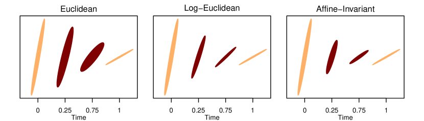
Figure 1: Comparison of three metric tensors on $\mathcal{SP}(2)$: Dark ellipses represent points at time $t=0.25,\,0.75$ on the geodesic connecting $P_{0}$ at $t=0$ and $P_{1}$ at $t=1$. The length of the axes are the square root of the eigenvalues.

The determinant of a covariance matrix measures the dispersion of the data points from a multivariate normal distribution. For the Euclidean metric, the geodesic connecting two fixed points often contains points with a larger determinant than the two fixed points, and the difference can get extremely large whenever the fixed points lie near the boundary of $\mathcal{SP}(n)$. This problem is referred to as the swelling effect [4, 23, 45]. In many contexts, the swelling effect is described as undesirable because the level of dispersion should remain close to the given information obtained by the observations of covariance matrices [4, 18, 30, 71]. The LE and AI metrics avoid this swelling effect. Moreover, points on LE and AI geodesics at corresponding times have the same determinants. These determinants are the result of linear interpolation in the logarithmic domain; this can be proved by following similar lines as in [4].

A visual illustration of the swelling effect is provided in Figure 1 where two intermediate points on the geodesic connecting

$$P_{0}=\begin{pmatrix}0.4&0.3\\ 0.3&0.4\end{pmatrix}\text{ at }t=0\,\,\,\,\text{ and }\,\,\,\,P_{1}=\begin{pmatrix}1&0.1\\ 0.1&0.02\end{pmatrix}\text{ at }t=1$$

are shown for each metric. Notice the swelling effect in the case of the Euclidean metric and also that the geodesic of the LE metric has points with exaggerated anisotropy; for more details on this phenomenon see [3, 23]. In general, whether anisotropy constitutes a problems depends on the application of interest.

fnum@section3 Stochastic processes on $\mathcal{SP}(n)$

fnum@subsection3.1 Overview

SDEs on manifolds present additional complications over the Euclidean setting which we deal with in three stages: firstly, we introduce the general notion of SDEs on manifolds. Secondly, we discuss Brownian Motion (definition, local representation, horizontal lift, construction via Euler-Maruyama with the exponential map and non-explosion) in subsection 3.2 and thirdly we proceed to the Ornstein–Uhlenbeck class in subsection 3.3.

Since the curvature of Riemannian manifolds makes direct use of Euclidean stochastic analysis prohibitively hard, a common strategy in stochastic analysis is to adopt the extrinsic view that involves embedding the manifold in a higher dimensional Euclidean space using the Nash embedding theorem; see for example, [39, 26, 31]. The approach benefits from existing theory for SDE’s on Euclidean space but a suitable coordinate system is often not explicitly available or too inconvenient, so this approach has limited practical use.

In this paper, we work with a probability space $(\Omega,\mathfrak{F},\mathbb{P})$ equipped with the filtration $\mathfrak{F}_{*}=\{\mathfrak{F}_{t},\,t\geq 0\}$ of $\sigma$-fields contained in $\mathfrak{F}$. Here, we assume that $\mathfrak{F}=\underset{t\uparrow\infty}{\lim}\mathfrak{F}_{t}$, while $\mathfrak{F}_{*}$ is right continuous and every null set (i.e. a subset of a set having measure zero) is contained in $\mathfrak{F}_{t}$.

On a Riemannian manifold $\mathcal{M}$ of dimension $d$, E. P. Hsu [39] writes the SDE driven by smooth vector fields $V_{0},\ldots,V_{l}$ by an $\mathbb{R}^{l+1}$-valued semi-martingale $Z_{t}$ (with initial condition $P\in\mathfrak{F}_{0}$) as

$$dX_{t}=\sum_{i=0}^{l}V_{i}(X_{t})\circ dZ^{(i)}_{t}\hskip 42.67912pt(X_{0}=P).$$ (7)

$Z^{(i)}_{t}$ could be a deterministic component, such as time, or a stochastic component, such as a Brownian motion: this corresponds to the usual distinction of some $V_{i}$ as drift and other $V_{i}$ as diffusivity. We call $X_{t}$ an $\mathcal{M}$-valued semi-martingale defined up to a $\mathfrak{F}_{*}$ stopping time $\tau$ if it satisfies

$$f(X_{t})=f(P)+\sum_{i=0}^{l}\int_{0}^{t}V_{i}f(X_{s})\circ dZ_{s}^{(i)}\hskip 28.45274pt0\leq t<\tau\,\,,\,\,f\in C^{\infty}(\mathcal{M}),$$ (8)

where the integrals above are in the Stratonovich sense, and converting them to Ito sense yields:

$$f(X_{t})=f(P)+\sum_{i=0}^{l}\int_{0}^{t}V_{i}f(X_{s})\,dZ_{s}^{(i)}+\frac{1}{2}\sum_{i,j=0}^{l}\int_{0}^{t}(\nabla_{V_{j}}V_{i})f(X_{s})\,d[Z^{(i)},Z^{(j)}]_{s}.$$ (9)

Here, $[Z^{(i)},Z^{(j)}]_{t}$ stands for the usual quadratic covariation of $Z_{t}^{(i)}$ and $Z_{t}^{(j)}$ defined on the Euclidean space. Comparing to equation (8), the additional terms in equation (9) arise from the non-trivial chain rule in the Ito case. The Stratonovich representation in equation (8) brings simplicity and is invariantly defined whence it is usually preferred for SDE’s on manifolds [26].

fnum@subsection3.2 Brownian motion class

Since the infinitesimal generator of Brownian motion on Euclidean space is $\Delta/2$, with $\Delta$ the usual Laplace operator, Brownian motion on a Riemannian manifold $\mathcal{M}$ can also be defined as a diffusion process generated by $\Delta_{\mathcal{M}}/2$ where $\Delta_{\mathcal{M}}$ denotes the Laplace-Beltrami operator. The resulting Brownian Motion $X_{t}$ can be expressed in local coordinates using the standard Brownian motion $B_{t}$ on $\mathbb{R}^{d}$ by writing $\Delta_{\mathcal{M}}$ in local coordinates:

$$dX_{t}^{i}=\sum_{j=1}^{d}(G^{-1/2})_{ij}(X_{t})\,dB_{t}^{(j)}-\frac{1}{2}\sum_{k,l=1}^{d}(G^{-1})_{lk}(X_{t})\,\Gamma_{kl}^{i}(X_{t})dt\hskip 28.45274pt1\leq i\leq d,$$ (10)

where $(G^{-1})_{ij}$ is the $(i,j)$-entry of $G^{-1}$ which is the matrix form of the metric tensor $g$ of the manifold $\mathcal{M}$, see [26, 39].

We choose to instead adopt the intrinsic viewpoint that studies Riemannian manifolds via their metric or connection which enables us to write down less cumbersome SDEs with more readily interpretable parameters. Thus, let us introduce a frame $u:\mathbb{R}^{d}\rightarrow T_{P}\mathcal{M}$ at $P\in\mathcal{M}$ (this is an isomorphism of vector spaces with inner product) and the frame bundle $\mathscr{F}(\mathcal{M})$ which is the collection of all frames for all $P\in\mathcal{M}$. Let us fix the standard basis $\{e_{i}\}_{i=1}^{d}$ on $\mathbb{R}^{d}$ and express $u$ in local coordinates $\{E_{1},\ldots,E_{d},e_{1},\ldots,e_{d}\}$ in some neighbourhood $U$ covering $P\in\mathcal{M}$ as $u=(P,\zeta)$ with $\zeta=(\zeta^{i}_{j})\in\mathbb{R}^{d\times d}$ the coefficients with respect to the orthonormal basis $\{E_{i}(Q)\}_{i=1}^{d}$ on $T_{P}\mathcal{M}$ for all $Q\in U$. This means that for any vector $e\in\mathbb{R}^{d}$ with coordinates $\epsilon_{i}$, i.e. $e=\sum_{i=1}^{d}\epsilon_{i}e_{i}\in\mathbb{R}^{d}$:

$$u(e)=\sum_{i,j=1}^{d}\epsilon_{i}\,\zeta_{j}^{i}\,E_{i}(P)\in T_{P}\mathcal{M}.$$

Moreover, $\mathscr{F}(\mathcal{M})$ is again a smooth manifold, and the canonical projection map $\pi:\mathscr{F}(\mathcal{M})\rightarrow\mathcal{M}$ is smooth [39]. If $u_{t}$ is a smooth curve on $\mathscr{F}(\mathcal{M})$ and for each $e\in\mathbb{R}^{d}$ the vector field $u_{t}(e)$ of $\mathcal{M}$ is parallel along the curve $\pi(u_{t})$, $u_{t}$ is called horizontal curve on $\mathscr{F}(\mathcal{M})$. For any smooth curve $\gamma$ on $\mathcal{M}$, there is a corresponding horizontal curve on $\mathscr{F}(\mathcal{M})$ (unique up to choice of initial condition $u_{0}$) which is referred to as the horizontal lift of $\gamma$. This definition carries over to the horizontal lift of a tangent vector on $\mathcal{M}$. We define the anti-development of $\gamma$ as

$$w_{t}=\int_{0}^{t}u_{s}^{-1}(\gamma^{\prime}(s))\,ds,$$

where $u_{t}$ is the horizontal lift of $\gamma(t)$ on $\mathcal{M}$. While this anti-developement $w_{t}$ is guaranteed to exist and is uniquely defined up to the initial conditions $u_{0}$ and $\gamma(0)$, its computation is often difficult. To address this issue, we establish the following:

Proposition 1.

On $\mathcal{SP}(n)$, in the case of the LE metric, the horizontal lift of a smooth curve can be explicitly expressed in local coordinates. For the AI metric, a first order Euler approximation for the horizontal lift of a geodesic can be explicitly computed.

More details about the stochastic development on $\mathcal{SP}(n)$ are discussed in Subsection S2 of the Supplementary Material.

By carrying out a similar process to the case of a smooth curve, we obtain a corresponding horizontal semi-martingale $U_{t}$ on the frame bundle and an anti-development $W_{t}$ on $\mathbb{R}^{d}$ to a semi-martingale $X_{t}$ on $\mathcal{M}$. Up to a choice of initial conditions, this relationship is one-to-one. The process of transforming $W_{t}$ to $X_{t}$ is called stochastic development [26]. One particularly important result is that one can define Riemannian Brownian motion on $\mathcal{M}$ with the connection $\nabla$ by having its anti-development $W_{t}$ be the standard Euclidean Brownian motion. On the sphere $\mathcal{S}^{2}$, stochastic development is intuitively described as “rolling without slipping”: if we have a path of Brownian motion $W_{t}$ on a flat paper (this paper acts as the tangent plane of $\mathcal{S}^{2}$), rolling the sphere along the path of $W_{t}$ without slipping results in a trajectory on $\mathcal{S}^{2}$ which turns out to be a path of the Riemannian Brownian motion on $\mathcal{S}^{2}$.

Yet another alternative construction of Riemannian Brownian Motion uses the Euler–Maruyama approximation, which employs the exponential map. We call thus method the exponential adapted Euler–Maruyama method, that is

$$X_{t+\delta t}=\text{Exp}_{X_{t}}\left\{\sum_{i=1}^{d}(B^{(i)}_{t+\delta t}-B^{(i)}_{t})\,E_{i}(X_{t})\right\}\hskip 14.22636pt\text{ for }\delta_{t}>0;$$ (11)

see for example, [10, 51, 53]. As $\delta t\rightarrow 0$, $X_{t}$ converges to the Riemannian Brownian motion in distribution if there exists a global basis field on the tangent bundle $\mathscr{F}(\mathcal{M})$, i.e. $\mathcal{M}$ is a parallelizable manifold [31, 53, 43]. Since $\mathcal{SP}(n)$ endowed with either the LE or the AI metric is geodesically complete (i.e. the exponential map is a global diffeomorphism) and parallelizable, the approximation method in equation (11) becomes more convenient and efficient in our case.

The transition density function $p_{\mathcal{M}}(s,P;t,Q)$ of the Riemannian Brownian motion exists but usually no explicit expression is available, while on the Euclidean space it is simply the Gaussian distribution [39, 26]. On the Euclidean space, Brownian motion does not explode in finite time, and if this holds in the Riemannian setting, that is

$$\int_{\mathcal{M}}p_{\mathcal{M}}(0,P;t,Q)\,dQ=1\hskip 28.45274pt\text{ for all }P\in\mathcal{M}\,\,\,\&\,\,\,\,0<t<\infty,$$

then the manifold $\mathcal{M}$ is said to be stochastically complete. It turns out that $\mathcal{SP}(n)$ equipped either with the LE or the AI metric is also stochastically complete, see Subsection S2 of the Supplementary Material.

fnum@subsection3.3 Ornstein–Uhlenbeck (OU) class

Adopting the intrinsic point of view, we present a construction of an OU class of processes on $\mathcal{SP}(n)$ for both the LE and the AI metrics. In analogy with the Euclidean OU process, we start with Brownian motion and add a mean-reverting drift which pushes the process toward the point of attraction. In the Euclidean setting, this drift is simply given as the gradient of the squared distance between the process and the point of attraction. We translate this idea to manifolds by using the covariant derivative in the place of the Euclidean gradient. This is similar to the treatment of the drift term by V. Staneva & L. Younes [69] for shape manifolds.

Let us define the OU process on $\mathcal{SP}(n)$ to be the solution of the following SDE with model parameters $\theta\in\mathbb{R}_{>0}$, $M\in\mathcal{SP}(n)$ and $\sigma\in\mathbb{R}_{>0}$ :

$$dX_{t}=-\frac{\theta}{2}\,\nabla_{X_{t}}\left\{d^{2}(X_{t},M)\right\}\,dt+F_{X_{t}}(\sigma\,dB_{t})\hskip 28.45274pt(X_{0}=P).$$ (12)

This uses the smooth function $F:\mathcal{SP}(n)\times\mathbb{R}^{d}\rightarrow\Gamma(T\,\mathcal{SP}(n))$ defined by:

$$F_{Q}(e)=\sum_{i=1}^{d}\epsilon_{i}\,E_{i}(Q)\,\,\,\text{ with }\,\,\,e=\sum_{i=1}^{d}\epsilon_{i}\,e_{i}\in\mathbb{R}^{d},\,Q\in\mathcal{SP}(n)\text{ and }d=\frac{n(n+1)}{2},$$ (13)

where $\{E_{i}\}_{i=1}^{d}$ is the orthonormal basis field on $T\,\mathcal{SP}(n)$ with respect to the given metric tensor. The following Proposition demonstrates that the covariant derivative chosen for the drift in the SDE (12) is explicitly computable; the proof is presented in Proposition S2.1 of the Supplementary Material.

Proposition 2 (Riemannian gradient of distance squared on $\mathcal{SP}(n)$).

1. (LE metric). The set $\mathfrak{B}^{\text{LE}}_{d}=\{E_{i}^{\text{LE}}\}_{i=1}^{d}$ is an orthonormal frame on the tangent bundle $T\mathcal{SP}(n)$, where for any $P\in\mathcal{SP}(n)$:

   $$E_{i}^{\text{LE}}(P)=\big{(}d_{\log P}\big{)}^{-1}(S_{i})=D_{\log P}\exp.S_{i}\,\,\,\,\text{ for }1\leq i\leq d.$$

   Moreover, the Riemannian gradient of distance squared for any fixed point $Q\in\mathcal{SP}(n)$ is $\Big{(}\nabla\text{d}^{2}_{\text{LE}}(P,Q)\Big{)}_{P}=-2D_{\log P}\exp.(\log Q-\log P)=-2\,\text{Log}_{P}^{\text{LE}}(Q).$

2. (AI metric). The set $\mathfrak{B}^{\text{AI}}_{d}=\{E_{i}^{\text{AI}}\}_{i=1}^{d}$ is an orthonormal frame on the tangent bundle $T\mathcal{SP}(n)$, where for any $P\in\mathcal{SP}(n)$:

   $$E_{i}^{\text{AI}}(P)=P^{1/2}\star S_{i}\,\,\,\,\text{ for }1\leq i\leq d.$$

   Moreover, the Riemannian gradient of distance squared for any fixed point $Q\in\mathcal{SP}(n)$ is $\Big{(}\nabla\text{d}^{2}_{\text{AI}}(P,Q)\Big{)}_{P}=-2\,\sum_{i=1}^{d}\left\langle\log(P^{-1/2}\star Q),S_{i}\right\rangle_{F}\,E_{i}^{\text{AI}}(P)=-2\,\text{Log}^{\text{AI}}_{P}(Q).$

The OU processes on $\mathcal{SP}(n)$ are obtained as the limit $\delta_{t}$ tends to zero of the exponential adapted Euler-Maruyama method:

$$X_{t+\delta_{t}}=\text{Exp}_{X_{t}}\Bigg{\{}-\frac{\theta}{2}\nabla_{X_{t}}\{d^{2}(X_{t},M)\}\,\delta_{t}+\sum_{j=1}^{d}(B^{(j)}_{t+\delta_{t}}-B^{(j)}_{t})\,\sigma\,E_{j}(X_{t})\Bigg{\}}\,\,\text{ for }\delta_{t}>0.$$ (14)

The selection of the basis fields plays an important role as they represent the horizontal lift of $X_{t}$ locally when using the piece-wise approximation method in equation (14).

For the LE metric, we define a global isometric diffeomorphism $\mathfrak{h}$, that allows us to constructively identify $\mathcal{SP}(n)$ with $\mathbb{R}^{d}$. Additionally, it characterizes the OU class of processes on $\mathcal{SP}(n)$ equipped with the LE metric as the image of the standard OU process on $\mathbb{R}^{d}$ under $\mathfrak{h}$, see Theorem 1 in which the proof is presented in Subsection S1 of the Supplementary Material. In turn, this permits establishing existence, uniqueness and non-explosion of the OU class for the LE metric.

We define $\mathfrak{h}=(\mathfrak{h}_{j}):\mathcal{SP}(n)\rightarrow\mathbb{R}^{d}$ with $e=\sum_{j=1}^{d}\epsilon_{j}\,e_{j}\in\mathbb{R}^{d}$ and $P\in\mathcal{SP}(n)$ as follows:

$$\mathfrak{h}_{j}(P)=\langle\log P,S_{j}\rangle_{F}\,\,\,(1\leq j\leq d)\,\,\,\,\text{ and }\,\,\,\,\mathfrak{h}^{-1}(e)=\exp\big{(}\sum_{j=1}^{d}\epsilon_{j}\,S_{j}\big{)}.$$ (15)

Theorem 1.

Suppose the process $X_{t}$ is the solution of the following SDE on $\mathcal{SP}(n)$ endowed with the LE metric, for $t\in[0,\tau)$ with a $\mathfrak{F}_{*}$-stopping time $\tau$:

$$dX_{t}=A(t,X_{t})\,dt+F_{X_{t}}\big{(}b(X_{t})\,dB_{t}\big{)}\hskip 56.9055pt(X_{0}=P),$$ (16)

where $A$ assigns smoothly for each $t\in[0,\tau)$ a smooth vector field $A(t,\cdot)$ on $\mathcal{SP}(n)$ and some smooth function $b:\mathcal{SP}(n)\rightarrow\mathbb{R}^{d\times d}$. Moreover, $B_{t}$ is $\mathbb{R}^{d}$-valued Brownian motion and the function $F$ is defined in Equation (13) associated with the basis $\mathfrak{B}_{d}^{\text{LE}}$. Then the problem of solving the SDE (16) on $\mathcal{SP}(n)$ is the same as solving the following SDE on $\mathbb{R}^{d}$ :

$$dx_{t}=a(t,x_{t})\,dt+\tilde{b}(x_{t})\,dB_{t}\hskip 59.75095pt(x_{0}=p),$$ (17)

Here, $p=\mathfrak{h}(P)$, $x_{t}=\mathfrak{h}(X_{t})$ hold for all $t\in[0,\tau)$ and smooth function $\tilde{b}$ is given by $\tilde{b}=b\circ\mathfrak{h}^{-1}$. In addition, smooth function $a=\big{(}a^{(j)}\big{)}$ is given by

$$a^{(j)}:[0,\tau)\times\mathbb{R}^{d}\rightarrow\mathbb{R},\hskip 28.45274pt\,(t,x_{t})\mapsto\big{\langle}D_{X_{t}}\log.A(t,X_{t}),S_{j}\big{\rangle}_{F}\,\,\,\,\,\text{ for all }1\leq j\leq d.$$

Solutions of (16) and (17) are in one-to-one correspondence. Therefore, the conditions for existence and uniqueness of the solution for the SDE (16) depend directly on the requirements that the drift and diffusivity of the SDE (17) satisfy on the Euclidean space, e.g. continuity and local Lipschitzness. Indeed, equating the drift and diffusivity of the SDE (16) with our OU process, the SDE (17) turns out to be a standard OU process on $\mathbb{R}^{d}$. Thus, most favourable properties that the OU process has on the Euclidean space will carry over to $\mathcal{SP}(n)$, such as existence and uniqueness of the solution and ergodicity. The transition probability density is explicitly available up to the Jacobian term involving the derivative of the matrix exponential.

Corollary 1.

SDE (12) has a unique solution and gives rise to an ergodic diffusion process on $\mathcal{SP}(n)$ in the LE case.

We conclude this section by establishing equivalent results for the AI case in a non-constructive manner. Although there is no simple diffeomorphism corresponding to $\mathfrak{h}$, $\mathcal{SP}(n)$ equipped with the AI metric is parallelizable. Therefore, equivalent results can be obtained for the AI case:

Proposition 3.

The existence and uniqueness theorem in [26, Theorem 2E, Page 121] is applicable to the OU process on $\mathcal{SP}(n)$ equipped with the AI metric. Moreover, this diffusion process is also non-explosive, see [26, Corollary 6.1, Page 131].

fnum@section4 Bayesian parameter estimation

We now focus on the Bayesian estimation of the parameters of the OU difussion processes on $\mathcal{SP}(n)$ when observations are collected at low frequency. We adopt the data augmentation MCMC computational strategy introduced by G. O. Roberts & O. Stramer [64] which requires data imputation through sampling from a diffusion bridge. We need to build diffusion bridge samplers that operate on $\mathcal{SP}(n)$ which, unlike the Euclidean case, have not been studied before. A common approach used in manifolds is to use embedding or local charts followed by an appropriate Euclidean method; see for example, [6, 68, 69], but this strategy is unsuitable when transitioning between charts is required and charts can be cumbersome to work with. We therefore develop a diffusion bridge sampler exploiting the exponential map and adopting an intrinsic viewpoint. In fact, by using Corollary 1 we can translate any existing method for the OU process from the Euclidean to the LE setting, so in the remainder of this section we will focus only on the AI metric where no such result exists. To deal with the data augmentation problem it is either assumed that $X_{t}$ has constant diffusivity, or that $X_{t}$ is transformed to a process of constant diffusivity, or existence of a process that is absolutely continuous to $X_{t}$ and its corresponding transition probability density need to be derived. In the case of the AI metric, at first glance the SDE seems to have constant diffusivity. However, due to the presence of curvature, the diffusivity part does depend on the position of the process $X_{t}$, hence straightforward algorithms from literature are not applicable. In fact, by looking at the local coordinate expression of the Riemannian Brownian motion on $\mathcal{SP}(n)$ equipped with the AI metric (substituting $G^{-1}$ in equation (5) and Christoffel symbols given in Lemma 1 into equation (10)), the dependence of the diffusivity on $X_{t}$ is evident as is the complexity of the resulting expressions. Furthermore, attempting to sample from this Euclidean SDE using the standard Euler-Maruyama method will lead to symmetric but non-positive definite matrices.

On the Euclidean space, B. Delyon & Y. Hu [22] and M. Schauer & F. Van Der Meulen et al. [66] suggest adding an extra drift term which guides the SDE solution toward the correct terminal point and leaves its law absolutely continuous with respect to the law of the original conditional diffusion process; the Radon-Nikodym derivative is available explicitly. This results in an easier simulation, much better MCMC mixing rate of convergence and no difficulty of computing acceptance probability when updating the proposal bridge. The additional drift is the gradient of the logarithm of the transition density of an auxiliary process $\tilde{X}_{t}$ which must have explicitly available transition probability density. In the manifold setting, we are aware of one attempt to use the above approach to sample diffusion bridges through local coordinates by S. Sommer et al. [68], but using the exponential map in this context is new. Motivated by these ideas, we construct a methodology that allow us to sample a diffusion bridge on $\mathcal{SP}(n)$ equipped with the AI metric using a guided proposal process.

We need to choose a proposal diffusion process, which has both an explicit transition probability density and an analytically tractable gradient of the log transition probability density due to the requirement in otaining the additional drift in the guided proposals SDE. The Wishart process is inappropriate because it does not have a closed form for its Riemannian gradient so we choose a diffusion process $\tilde{X}_{t}$ on $\mathcal{SP}(n)$ with transition probability the Riemannian Gaussian distribution [65] given as

$$p(s,\tilde{X}_{s};t,\tilde{X}_{t})=\frac{1}{K_{n}(\sigma)}\,\exp\left(-\frac{\text{d}_{\text{AI}}^{2}(\tilde{X}_{s},\tilde{X}_{t})}{2\,(t-s)\,\sigma^{2}}\right),$$

where $K_{n}(\sigma)$ is the normalising constant that depends only on $\sigma$ and $n$. We emphasize that explicit availability of the guided proposal SDE is not actually a pre-requisite for the guided proposals algorithm. Indeed, the proposal Markov process $\tilde{X}_{t}$ exists but its SDE form is not explicitly available [10].

Consider the OU process $X_{t}$ on $\mathcal{SP}(n)$ equipped with the AI metric with its law $\mathbb{P}_{t}$ and assume that sampling from the target diffusion bridge $X_{t}^{*}=\{X_{t},0\leq t\leq T\,|\,X_{0}=U,X_{T}=V\}$ with its corresponding law $\mathbb{P}^{*}_{t}$ is required. We introduce the guided proposal $X_{t}^{\diamond}$ which is the solution of the following SDE with its law $\mathbb{P}^{\diamond}_{t}$:

$$dX^{\diamond}_{t}=\left(\theta\,\text{Log}^{\text{AI}}_{X^{\diamond}_{t}}\,M+\frac{\text{Log}_{X^{\diamond}_{t}}^{\text{AI}}\,V}{T-t}\right)\,\,dt+F(X^{\diamond}_{t})(\sigma\,dB_{t})\hskip 42.67912pt(X^{\diamond}_{0}=U).$$ (18)

We then show that $\mathbb{P}_{t}^{*}$ and $\mathbb{P}_{t}^{\diamond}$ are equivalent up to time $T$ with the aid of Lemma 1 and Lemma 2 in Theorem 2; proofs are shown in Subsection S2 of the Supplementary Material.

Lemma 1.

The Christoffel symbols at any $P\in\mathcal{SP}(n)$ with respect to the basis $\mathfrak{B}_{d}^{\text{AI}}$ do not depend on $P$ and are given by $\Gamma_{ij}^{k}(P)=\left\langle-(S_{i}S_{j}+S_{j}S_{i})\,,\,S_{k}\right\rangle_{F}/2$.

Lemma 2.

The Laplace-Beltrami operator $\Delta_{\mathcal{SP}(n)}$ and the Hessian to the squared Riemannian distance with respect to $\mathfrak{B}_{d}^{\text{AI}}$ equal to $2\,I_{d}$, that is

$$(\text{Hess}f)_{P}\big{(}E_{i}^{\text{AI}},E_{j}^{\text{AI}}\big{)}=2\,\delta_{ij}\hskip 8.5359pt\&\hskip 8.5359pt\Delta_{\mathcal{SP}(n)}f\big{(}E_{i}^{\text{AI}},E_{j}^{\text{AI}}\big{)}=2\,\delta_{ij}\hskip 28.45274pt\text{ for all }1\leq i,j\leq d.$$

where $f(P)=d^{2}_{\text{AI}}(P,Q)$ and $\delta_{ij}$ is the Kronecker delta.

Theorem 2.

For $t\in[0,T)$ the laws $\mathbb{P}_{t}$,$\mathbb{P}_{t}^{\diamond}$ and $\mathbb{P}_{t}^{*}$ are absolutely continuous. Let $p(t,X_{t};T,V)$ be the true (unknown) transition density of moving from $X_{t}$ at time $t$ to $V$ at time $T$ and let $X^{\diamond}_{[0:t]}$ be the path of $X_{t}^{\diamond}$ from time $0$ to $t$. Then

$$\frac{d\mathbb{P}_{t}}{d\mathbb{P}_{t}^{\diamond}}\big{(}X^{\diamond}_{[0:t]}\big{)} =\frac{\exp\big{(}f(X^{\diamond}_{0};\sigma^{2})\big{)}}{\exp\big{(}f(X^{\diamond}_{t};\sigma^{2})\big{)}}\exp\Big{\{}\Phi(t,X^{\diamond}_{[0:t]})+\phi\big{(}t,X^{\diamond}_{[0:t]}\big{)}\Big{\}},$$ (19)

$$\frac{d\mathbb{P}_{t}^{*}}{d\mathbb{P}_{t}^{\diamond}}\big{(}X^{\diamond}_{[0:t]}\big{)} =\frac{p(t,X_{t}^{\diamond};T,V)}{\exp\big{(}f(X^{\diamond}_{t};\sigma^{2})\big{)}}\,\frac{\exp\big{(}f(X^{\diamond}_{0};\sigma^{2})\big{)}}{p(0,U;T,V)}\exp\Big{\{}\Phi\big{(}t,X^{\diamond}_{[0:t]}\big{)}+\phi\big{(}t,X^{\diamond}_{[0:t]}\big{)}\Big{\}},$$ (20)

where the functions $f,\,\phi$ and $\Phi$ are defined by

$$f(X^{\diamond}_{t};\sigma^{2})=-\frac{d^{2}_{\text{AI}}(X^{\diamond}_{t},V)}{2\sigma^{2}(T-t)}=-\frac{\left|\left|\log\left((X^{\diamond}_{t})^{-1/2}V(X^{\diamond}_{t})^{-1/2}\right)\right|\right|_{F}^{2}}{2\sigma^{2}(T-t)},$$ (21)

$$\phi\big{(}t,X^{\diamond}_{[0:t]}\big{)}=\sum_{i,j=1}^{d}\int_{0}^{t}\frac{\big{(}\zeta^{i}_{j}(X_{s}^{\diamond};\Theta)\big{)}^{2}\,}{2(T-s)}\,ds,$$ (22)

$$\Phi\big{(}t,X^{\diamond}_{[0:t]}\big{)}=\int\limits_{0}^{t}\Bigg{(}\frac{\theta\,g_{X_{s}}^{\text{AI}}\left(\text{Log}^{\text{AI}}_{X^{\diamond}_{s}}M,\text{Log}^{\text{AI}}_{X_{s}^{\diamond}}V\right)}{\sigma^{2}(T-s)}$$

$$+\sum_{i,j,r=1}^{d}\,\frac{g_{X_{s}^{\diamond}}^{\text{AI}}\Big{(}\zeta_{j}^{i}(X_{s}^{\diamond};\Theta)\big{(}\sum_{l=1}^{d}\zeta_{l}^{i}(X_{s}^{\diamond};\Theta)\Gamma_{jl}^{r}+\big{(}E_{j}^{\text{AI}}\zeta_{r}^{i}(\cdot;\Theta)\big{)}_{X_{s}^{\diamond}}\big{)}E_{r}^{\text{AI}}(X_{s}^{\diamond})\,,\,\text{Log}^{\text{AI}}_{X_{s}^{\diamond}}V\Big{)}}{2(T-s)}\Bigg{)}ds,$$ (23)

with $\Gamma_{jl}^{r}$ given in Lemma 1. The functions $\zeta(X_{s}^{\diamond};\Theta)=\big{(}\zeta_{j}^{i}(X_{s}^{\diamond};\Theta)\big{)}$ are the coefficients with respect to the basis $\mathfrak{B}^{\text{AI}}_{d}$ in the local expression of the horizontal lift, see Proposition 1.

Note that all terms dependent on $\zeta$ are not independent of the model parameters $\Theta$. When the parameters change, the diffusion path $X^{\diamond}_{t}$ also changes, even when the Brownian motion driving this process remains unchanged. In other words, there are implicit dependencies between $\zeta$ and the model parameters $\Theta$. Hence, for clarification purposes, the function $\zeta$ is written as $\zeta(X_{s}^{\diamond};\Theta)$. In fact, we should understand $X^{\diamond}_{t}$ as a function that depends on the driving Brownian motion and model parameters. The Radon-Nikodym derivatives in equations (19)–(20) can not be computed explicitly due to the presence of $\zeta$. However, we can approximate $\phi$ and $\Phi$ in Theorem 2 based on the approximation of $\zeta$, see Corollary S2.6 of the Supplementary Material. As a result, Remark 1 is a crucial step to make our proposed algorithm practicable; detailed calculation of the approximation of $\phi$ and $\Phi$ are presented in Corollary S2.7 of the Supplementary Material.

Remark 1.

Suppose that we have an $\mathcal{SP}(n)$-valued path $\{X_{t_{k}}^{\diamond}=y^{\diamond}_{t_{k}}\}_{k=0}^{m+1}$ of the OU process $X_{t}$ when equipping $\mathcal{SP}(n)$ with the AI metric, in which it is simulated from the exponential adapted Euler-Maruyama method, see Equation (14), where $\max\{t_{k+1}-t_{k}\}_{k=0}^{m}$ is sufficiently small and $0=t_{0}<\ldots<t_{m+1}=t$. Then the functions $\phi$ in Equation (22) and $\Phi$ in Equation (23) can be approximated as follows:

$$\phi(t,X^{\diamond}_{[0:t]}) \approx\frac{d}{2}\log\frac{T-t}{T},$$ (24)

$$\Phi(t,X^{\diamond}_{[0:t]}) \approx\sum_{k=0}^{m}\frac{t_{k+1}-t_{k}}{T-t_{k}}\,\Bigg{\{}\frac{\theta\,\left\langle\log\big{(}(y_{t_{k}}^{\diamond})^{-1/2}\star M\big{)}\,,\,\log\big{(}(y_{t_{k}}^{\diamond})^{-1/2}\star V\big{)}\right\rangle_{F}}{\sigma^{2}}$$

$$\hskip 28.45274pt+\frac{\left\langle\Gamma\,,\,\log\big{(}(y_{t_{k}}^{\diamond})^{-1/2}\star V\big{)}\right\rangle_{F}}{2}\Bigg{\}},$$ (25)

with $\Gamma=\sum_{i,r=1}^{d}\Gamma_{ii}^{r}S_{r}$ and the Christoffel symbols $\Gamma_{ii}^{r}$ are given in Lemma 1.

We expect that taking the limit $t\uparrow T$ in equation (20) will follow along similar lines to those in [22] and [66] so that the following holds

$$\frac{d\mathbb{P}_{T}^{*}}{d\mathbb{P}_{T}^{\diamond}}(X^{\diamond}_{[0:T]})=\frac{\mathcal{H}_{n,T}}{p(0,U;T,V)}\,\exp\left\{f(X^{\diamond}_{0};\sigma^{2})+\Phi(T,X^{\diamond}_{[0:T]})-\frac{d}{2}\log\sigma^{2}\right\}\,,$$

where $\mathcal{H}_{n,T}$ is a fixed scalar that depends only on the dimension $n$ and the terminal time $T$. While we do not present the full argument, we do, however, provide a careful numerical validation in Section 5.

Suppose we have discretely observed data $\mathfrak{D}=\{X_{t_{j}}=y_{j}\}_{j=0}^{N}$ at observation times $t_{0}=0<t_{1}<\cdots<t_{N}=T$, where the diffusion process $X_{t}$ is the OU process $X_{t}$ on $\mathcal{SP}(n)$. We aim to sample from the posterior distribution of $\Theta=\{\theta,\,M,\sigma^{2}\}$. We set $\mu=\sum_{i=1}^{d}\mu^{(i)}\,e_{i}=\mathfrak{h}(M)$, as defined in equation (15), and the prior distributions of $\{\theta,\mu,\sigma^{2}\}$ as $\pi_{0}^{\theta},\,\pi_{0}^{\mu}$ and $\pi_{0}^{\sigma}$ respectively. The key step involves first imputing suitable $m_{j}-1$ data points between the $j\text{th}$ consecutive observations in a way that they are independent of the diffusivity, and then employing the exponential adapted Euler–Maruyama method for the likelihood approximation. We choose to use random walk symmetric proposal distributions with suitable choices of step size $q(\tilde{\theta}|\theta),\,q(\tilde{\mu}|\mu)$ and $q(\tilde{\sigma}^{2}|\sigma^{2})$ for $\{\theta,\mu,\sigma^{2}\}$ respectively.

Algorithm 1 (Guided proposals on $\mathcal{SP}(n)$).

1. (Iteration $k=0$). Choose starting values for $\Theta$ and sample standard Brownian motions $W_{j}$, independently for $1\leq j\leq N$, each covering the time interval $t_{j}-t_{j-1}$, and set $B_{j}^{(0)}=W_{j}$.

2. (Iteration $k\geq 1$).

   1. Update $B_{j}$ independently $(1\leq j\leq N)$: sample the proposal $\tilde{W}_{j}$ and obtain $\tilde{Y}_{[t_{j-1},t_{j}]}$ from $\{\tilde{W}_{j},\theta_{k-1},M_{k-1},\sigma^{2}_{k-1},\mathfrak{D}\}$ and $Y_{[t_{j-1},t_{j}]}$ from $\{B_{j}^{(k-1)},\theta_{k-1},M_{k-1},\sigma^{2}_{k-1},\mathfrak{D}\}$ using equation (14) to approximately solve the SDE (18); then accept $\tilde{W}_{j}$ with probability

      $$\alpha^{(B)}=\min\left\{1,\exp\left[\Phi(t_{j}-t_{j-1},\tilde{Y}_{[t_{j-1},t_{j}]})-\Phi(t_{j}-t_{j-1},Y_{[t_{j-1},t_{j}]})\right]\right\}.$$

   2. Sample $\tilde{\sigma}^{2}$ from $q(\sigma^{2}|\sigma_{k-1}^{2})$ and obtain $\tilde{Y}_{[t_{j-1},t_{j}]}$ from $\{B_{j}^{(k)},\theta_{k-1},M_{k-1},\tilde{\sigma}^{2},\mathfrak{D}\}$ and $Y_{[t_{j-1},t_{j}]}$ from $\{B_{j}^{(k)},\theta_{k-1},M_{k-1},\sigma^{2}_{k-1},\mathfrak{D}\}$ using equation (14) to approximately solve the SDE (18); then accept $\tilde{\sigma}^{2}$ with probability

      $$\alpha^{(\sigma)} = \min\Bigg{\{}1,$$

      $$\frac{\pi_{0}^{\sigma}(\tilde{\sigma}^{2})\cdot\prod_{j=1}^{N}\exp\left\{\Phi(t_{j}-t_{j-1},\tilde{Y}_{[t_{j-1},t_{j}]})+f(\tilde{Y}_{t_{j-1}},\tilde{\sigma}^{2})-\frac{d}{2}\tilde{\sigma}^{2}\right\}}{\pi_{0}^{\sigma}(\sigma^{2}_{k-1})\cdot\prod_{j=1}^{N}\exp\left\{\Phi(t_{j}-t_{j-1},Y_{[t_{j-1},t_{j}]})+f(Y_{t_{j-1}},\sigma_{k-1}^{2})-\frac{d}{2}\sigma^{2}_{k-1}\right\}}\Bigg{\}}.$$

   3. Update $\mu$ and $M$ : sample $\tilde{\mu}$ from $q(\mu|\mu_{k-1})$, compute the corresponding $\tilde{M}=\mathfrak{h}^{-1}(\tilde{\mu})$ and accept $\tilde{\mu}$, $\tilde{M}$ with probability

      $$\alpha^{(M)}=\min\Bigg{\{}1,\frac{\pi_{0}^{\mu}(\tilde{\mu})}{\pi_{0}^{\mu}(\mu_{k-1})}\, \exp\bigg{\{}\sum_{j=1}^{N}\Big{[}\Phi\left(t_{j}-t_{j-1},\tilde{Y}_{[t_{j-1},t_{j}]}\right)$$

      $$-\Phi\left(t_{j}-t_{j-1},Y_{[t_{j-1},t_{j}]}\right)\Big{]}\bigg{\}}\Bigg{\}},$$

      where $\tilde{Y}_{[t_{j-1},t_{j}]}$, $Y_{[t_{j-1},t_{j}]}$ are from $\{B_{j}^{(k)},\theta_{k-1},\tilde{M},\sigma^{2}_{k},\mathfrak{D}\}$, $\{B_{j}^{(k)},\theta_{k-1},M_{k-1},\sigma^{2}_{k},\mathfrak{D}\}$ respectively using equation (14) to approximately solve the SDE (18).

   4. Update $\theta$ similarly as $\mu$.

Remark 2 (Time change).

Since $\Phi$ in equation (23) explodes as $t\uparrow T$, M. Schauer & F. Van Der Meulen et al. [66] suggests time change and scaling to reduce the required number of imputed data points. Scaling will not be as effective here as in the univariate setting because it can only fit one of the directions involved, so the effect is less pronounced than in the univariate setting and we expect further lessening as dimension increases. Nonetheless, in this work, we adopt one time change function from [66] which maps $s$ to $s\,(2-s/T)$.

fnum@section5 Simulation study on $\mathcal{SP}(2)$

p-values of K-S tests
		$\epsilon$
		$0.2$	$0.1$	$0.05$
Determinant	$m=1000$	0.00412	0.0329	0.288
	$m=2000$	0.00283	0.0612	0.370
Trace	$m=1000$	0.0112	0.0293	0.108
	$m=2000$	0.00123	0.0378	0.288

Table 2: Comparison in distribution at $t=T/2$ of the true bridges and the guided proposal bridges, given that $U$ and $V$ are chosen as in Case 1. Top table: p-values from the Kolmogorov–Smirnov (K-S) tests, where $\epsilon$ and $m$ are varied. Bottom figures: the Q-Q plots for determinant and trace when $m=2000$ and $\epsilon=0.05$.

fnum@subsection5.1 Brownian bridges

We perform a simulation exercise to illustrate our proposed bridge sampling of Algorithm 1 and to compare the performance for the Euclidean, LE and AI metrics. The simulation scenario involves sampling a standard Brownian bridge $W_{t}$ conditioned on $\{W_{0}=U,W_{T}=V\}$, $T=0.1$, $n=2$, in two cases: (i) with $U$ and $V$ lying far away from the boundary, $U=\begin{pmatrix}2&1\\ 1&2\end{pmatrix}$, and $V=\begin{pmatrix}3&1\\ 1&2\end{pmatrix}$ and (ii) with $U$ and $V$ lying close to the boundary, $U=\begin{pmatrix}2&1.999\\ 1.999&2\end{pmatrix}$, $V=\begin{pmatrix}3&2.435\\ 2.435&2\end{pmatrix}$. For the Euclidean metric we simply embed $\mathcal{SP}(n)$ in $\mathcal{S}(n)$ endowed with the Frobenius inner product and thus the Brownian motion in this case is the solution of the SDE $d\nu(W_{t})=dB_{t}\,\,(W_{0}=U)$, where $B_{t}$ is the standard Brownian motion on $\mathbb{R}^{d}$ and $\nu(W_{t})\in\mathbb{R}^{d}$ contains only independent entries of $W_{t}$. The LE and AI metrics are based on Theorem 1 and Algorithm 1 respectively.

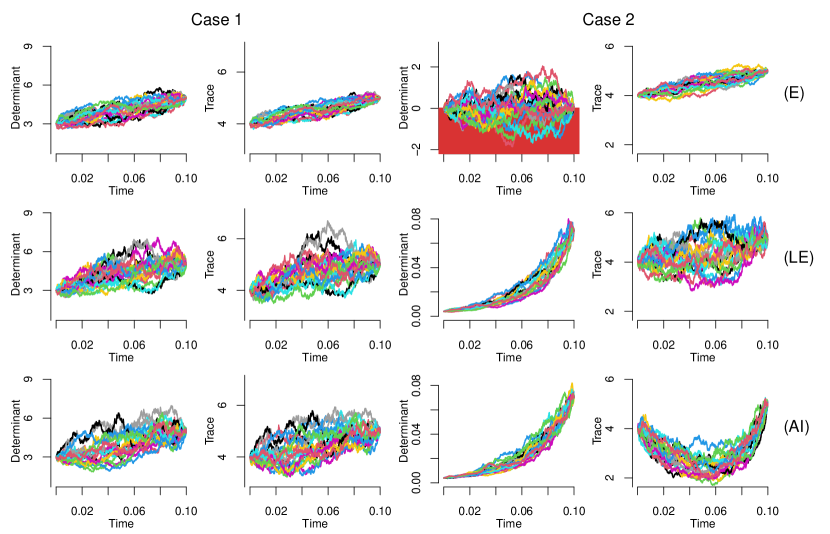
Figure 2: Time series for determinant and trace of 20 simulated Brownian bridges on $\mathcal{SP}(2)$ endowed with three different metrics (Euclidean: top row, Log Euclidean: middle row, Affine Invariant: bottom row) in the $2$ cases (i) and (ii). Red background area shows failure to be positive definite.

First we evaluate how Algorithm 1 performs compared with the naive simulation approach. For case (i) we obtain samples by forward-simulating the guided proposal in equation (18) and accepting with probability $\alpha^{(B)}$ in Algorithm 1. We then compare these bridges with the so-called true bridges, which are generated from the naive simulation approach by forward-solving the Riemannian Brownian motion $X_{t}$ and picking only those paths $X_{t}$ that satisfy $\text{d}_{\text{AI}}(X_{0.1},V)<\epsilon$ for some $\epsilon>0$. For different values of $\epsilon$ and number of imputed points $m$, we collect $1000$ sampled bridges and carry out a Kolmogorov–-Smirnov (K-S) test to compare the distribution of the true and approximated bridges at $t=T/2=0.05$; The Q-Q plots and the K-S p-values shown in Table 2 indicate that the values $m=2000,\epsilon=0.05$ provide a good approximation and as $\epsilon\downarrow 0$ the two distributions get closer to each other. Note that for case (ii) we had a difficulty in sampling true bridges because $V$ is too close to the boundary of $\mathcal{SP}(2)$ and points on the boundary are at infinite distance to covariance matrices. This difficulty escalates as dimension $n$ increases. Beside high dependence with the diffusivity, the naive approach of simulating bridges has very low acceptance rate when the conditioned observation is close to being non-positive definite, thus it is clearly not a good approach to use in the data-augmentation algorithm.

Next, we illustrate the problems that arise when neglecting the geometric structure of $SP(n)$ as stated in Section 2.2. Figure 2 depicts traces and determinants of $20$ simulated bridges with each metric. First note that the Euclidean metric samples do not achieve positive definiteness and have a clear presence of the swelling effect. The LE and AI metrics sample points that lie in $\mathcal{SP}(n)$ while the determinants behave reasonably with respect to the conditional points. In fact, one can show following the lines of the case of geometric means in [4] that the distribution of the determinant is the same for the LE and the AI metrics. The AI metric leads to less anisotropy that becomes more noticeable when the conditional points have eigenvalues close to zero, see plots about the trace in Fig. 2, indicating that the selection between LE and AI depends on the desirable property that one wishes to achieve.

fnum@subsection5.2 Parameter estimation for the Affine-Invariant metric

5.2.1 Dimension $n=2$

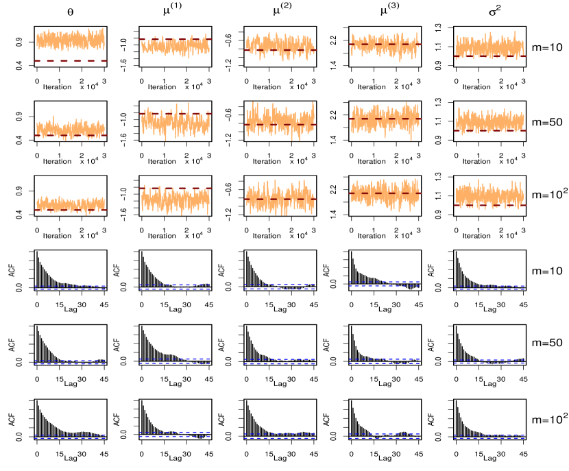
Figure 3: (Simulation study). $m$ is varied over $10,\,50$ and $100$. Top three rows: Traceplots from $4\times 10^{3}$ iterates after discarding $10^{3}$ iterations of burn-in, where true values are indicated with the red dashed lines. Bottom three rows: ACF plots based on these MCMC chains.

We simulate $10^{6}+1$ equidistant time points $X_{t}$ of the OU process in the case of the AI metric on $[0,100]$ using equation (14) with model parameters $\theta=0.5$, $M=\left(\begin{array}[]{cc}1&0.9\\ 0.9&1\end{array}\right)$, $\sigma^{2}=1$ and $X_{0}=I_{2}$ and take sub-samples at time points $\{0,0.2,\ldots,100$}. We apply the Algorithm 1 with time change assuming the prior distributions $\log\sigma^{2},\,\log\theta\sim N(0,4)$ and $\mu\sim N(0,4\times I_{3})$.

Figure 3 is based on 1,000 burn-in and 4,000 MCMC iterations; it indicates that increasing $m$ does not affect the mixing of the chain and improves, in some cases, the approximation to the marginal densities. We then run a longer MCMC chain of $50000$ iterations while varying the value of $m$ over $10,\,50,\,100$ and $200$. These chains are thinned out after a burn-in period of $2000$ iterations and samples of $4000$ points are collected from the target distributions. Figure 4 shows that the kernel density estimations of the marginal posterior distributions of $\{\theta,\,\mu,\,\sigma^{2}\}$ are approximately the same for $m=100,\,200$. Thus, $m=100$ is considered to provide a sufficiently fine discretization for these data. The average proportions of accepting the bridges after the burn-in period are $72.7\%,70.2\%,68.5\%$ and $67.3\%$ for $m=10,50,100$ and $200$ respectively.

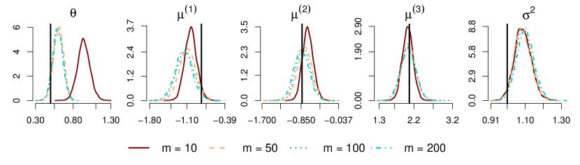
Figure 4: (Simulation study). Estimated posterior distribution of $\{\theta,\mu,\sigma^{2}\}$ using $5\times 10^{4}$ MCMC iterations ($2\times 10^{3}$ burn-in discarded, thinned by $12$), and the result for $M=\mathfrak{h}^{-1}(\mu)$ is given in Figure S1 (Supplementary material). True values are indicated by solid vertical black lines.

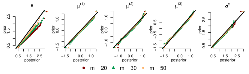
Figure 5: Prior reproduction test to validate the Algorithm 1 with time change: Q-Q plots of priors against posteriors from three model parameters.

Our final investigation for Algorithm 1 is the prior reproduction test of S. R. Cook et al. [20] to validate the Algorithm 1. We assume proper priors for $\{\theta,\mu,\sigma^{2}\}$ : $\log\theta,\,\log\sigma^{2}\sim N(0,0.3^{2}),\,\mu\sim N(0,0.2\times I_{3})$ and $n=500$.

We generate, in turn, $1000$ samples from the prior distributions and then, conditional on each sampled parameter vector, high-frequency observations on $[0,50]$ at $5\times 10^{5}+1$ equidistant time points and keep sub-samples at time points $\{0,0.1,\ldots,50\}$. For the $1000$ generated datasets we estimate the corresponding posterior densities using Algorithm 1 and test whether they come from the same distribution as the prior as this validates that our algorithm works properly. Figure 5 illustrates that the prior has been successfully replicated while, as expected, the parameters approximation improves as $m$ increases.

5.2.2 Higher dimensions

Since there are $n(n+1)/2$ diffusions to estimate, the computational cost of Algorithm 1 will grow proportionally to $n^{2}$. In this subsection, we present a comparison of the performance of the Algorithm in dimensions $n=2$ and $n=3$. We used compiled C++ code in R on a PC running at 2290 MHz with 16 cores. For each dimension, we monitored the times of the central processing unit (CPU) for $10^{4}$ iterations after suitable burn-in periods and reported the average times per iteration.

Similarly to the case of dimension $n=2$, we simulated $10^{6}+1$ time points on $[0,100]$ with model parameters

$$\theta=0.5\,;\hskip 28.45274ptM=\begin{pmatrix}1&0.7&0.9\\ 0.7&1.2&0.9\\ 0.9&0.9&1\end{pmatrix}\,;\hskip 28.45274pt\sigma^{2}=1,$$

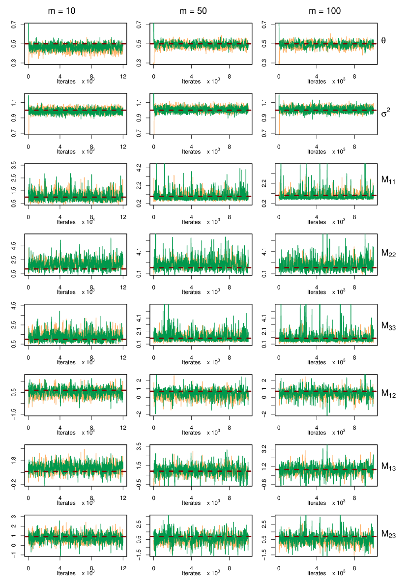
Figure S4: (Simulation study on $\mathcal{SP}(3)$). MCMC traceplots of $12\times 10^{3}$ iterations using different start points (orange, green) when number of imputed points $m$ are varied over $10,\,50$ and $100$.

and assumed the prior distributions $\log\sigma^{2},\,\log\theta\sim N(0,4)$ and $\mu\sim N(0,4\times I_{6})$ and number of imputed points $m$ varying over $10,\,50$ and $100$. Traceplots from $10^{4}$ iterations after discarding $2\times 10^{3}$ iterations of burn-in and the corresponding ACF plots can be found in Figures S4 and S5 (Supplementary material).

Number of imputed points	Dimension	CPU times per iterations (seconds)
$m=10$	$n=2$	0.0596
	$n=3$	0.408
$m=50$	$n=2$	0.288
	$n=3$	2.08
$m=100$	$n=2$	0.541
	$n=3$	4.27

Table 3: Average CPU times per iterations after suitable burn-in period when using Algorithm 1.

Table 3 indicates that working with dimension $n=3$ requires more computational resources. In fact, it takes roughly 7 times longer to run for all three cases of $m\in\{10,50,100\}$ compared to when working with dimension $n=2$. However, the MCMC running time is still entirely manageable, even in the case of imputing the highest number of points $m=100$. Illustrations for the convergence of the MCMC chains for dimension $n=3$ are shown in Figures S4 and S5 (Supplementary material).

fnum@section6 Application to finance

fnum@subsection6.1 Introduction

The widespread availability of intra-day high-frequency prices of financial assets has enabled the computation of consistent estimates of daily covariation of asset prices called realized covariances, introduced in [1, 2] and studied in detail by O. E. Barndorff-Nielsen & N. Shephard [7]. The literature in discrete time series involves approaches based on Wishart-based distributions, see [5, 33, 36, 41, 74, 42]; matrix decompositions to deal with the positive definiteness requirement of the elements of the covariance matrices, see [9, 19]; or ideas borrowed from the literature of multivariate GARCH models, see [58, 37]. There has been quite a lot of evidence that direct modelling of realized covariances provides more precise forecasts than GARCH and stochastic volatility multivariate models that assume that the covariance matrices are unobserved latent matrices; see [33, 36, 19, 9, 58, 33].

One important practical question in this framework is how covariance matrices vary at different time scales. It is well known since the paper by T. W. Epps [27] that correlations between assets decrease with the duration of investment horizons and this necessitates models that are frequency independent. Modelling realized covariances with diffusions offers a critical advantage over discrete time models because they allow inference of implied model dynamics and properties as well as forecasting at various frequencies that may differ from the observed data frequency. Moreover, continuous time models are useful in irregularly spaced observed data and provide a clear advantage when used in pricing derivative instruments.

fnum@subsection6.2 Data preprocessing

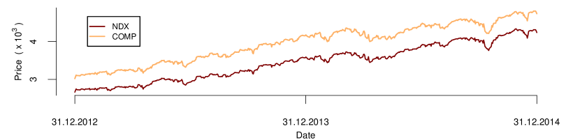
Figure 6: Time series of the closing price from two indices: NASDAQ Composite (COMP) and NASDAQ $100$ (NDX) at the end of each working day from $31.12.2012$ to $31.12.2014$.

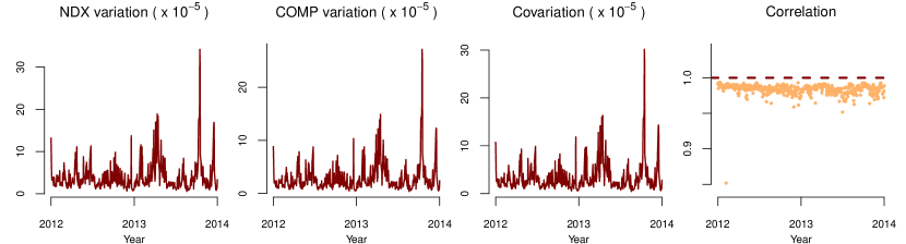
Figure 7: Time series of estimated covariance matrices based on the price of two indices NDX and COMP. Estimated correlations between indices are plotted against time (red dashed line indicates correlation $1$).

We estimate $2\times 2$ daily covariance (volatility) matrices from NASDAQ Composite (COMP) and NASDAQ $100$ (NDX) indices with data of $504$ working days obtained from $31.12.2012$ to $31.12.2014$ at $1-$minute intervals from [29]; see Figure 6. For the estimation we used quadratic variation/covariation in the logarithm domain and assumed that the microstructure noise does not impact our estimates because the indices are very liquid [75]. We verified this assumption by noting that estimates based on $5$-minute inter-observation intervals are very similar.

The pattern of the time series from the entries of covariance matrices in Figure 7 indicates a mean-reverting tendency and many observations lying close to the boundary of $\mathcal{SP}(2)$, making the Euclidean metric inappropriate and the Riemannian structures suitable.

fnum@subsection6.3 Model fitting

Our time series has unevenly spaced observations due to weekends and holidays, so the imputed points $m_{j}$ between the $(j-1)\text{th}$ and $j\text{th}$ consecutive observations are carefully chosen such that $\delta_{t}=(t_{j}-t_{j-1})/m_{j}$ is constant. We choose vague proper priors $\log\theta\sim N(0,4)$ , $\log\sigma^{2}\sim N(-1,4)$ and $\mu\sim N\left(\left(\begin{array}[]{ccc}-12&-12&3\end{array}\right)^{T},4\,I_{3}\right)$. We adopt the algorithm by G. O. Roberts & O. Stramer [64] in the case of the LE metric and Algorithm 1 with time change for the case of the AI metric. Trace plots and ACF plots when using either the LE metric with $\delta_{t}=0.01$ or the AI metric with $\delta_{t}=0.001$ are shown in Figure S2 (Supplementary Material). MCMC samples based on $10^{5}$ iterations with varying values of $\delta_{t}$ were collected after a burn-in period of 4000 iterations and kernel density estimations are depicted in Figure 8.

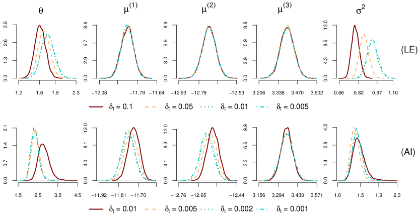
Figure 8: Estimated posterior distribution for $\{\theta,\mu,\sigma^{2}\}$ from financial data example using either the LE (top row) or the AI metric (bottom row), based on $10^{5}$ MCMC iterations ($4\times 10^{3}$ burn-in discarded, thinned by $19$). Moreover, the result for $M=\mathfrak{h}^{-1}(\mu)$ is given in Figure S3 (Supplementary material).

Fewer imputed points are required for the LE metric than for the AI metric to adequately approximate the posterior densities which we attribute to different degrees of non-linearity: after transformation through the matrix logarithm, the LE problem is reduced to a linear problem whereas with the AI metric, discretization including approximation of the horizontal lift takes place in the original domain. This domain can be seen to be less linear from the fact that covariance matrices are commutative under the logarithm product which is at the heart of the LE metric whereas exchanging the order of multiplication causes a different result for the AI metric. This difference is more pronounced near the boundary of the cone which is where the majority of our observations lie.

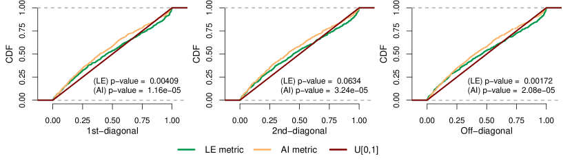
Figure 9: Empirical cumulative distribution of the generalized residuals for the entries from volatilities under two models using either the LE and the AI metric, in which model parameter estimates are the posterior mean. Moreover, p-values are obtained from the K-S tests of comparison to $U[0,1]$ (red line).

We test the fit of the two models using the transition density-based approach by Y. Hong & H. Li [38]. For each model, we choose the posterior mean to estimate $\{\theta,M,\sigma^{2}\}$ and compute the generalized residuals $Z_{j}^{(i)}$, for $1\leq j\leq 504$, as

$$Z_{j}^{(i)}=\int_{-\infty}^{y_{j}^{(i)}}p^{(i)}(t_{j},v|t_{j-1},y_{j-1})dv.$$ (26)

where $\{y_{j}^{(i)}\}_{j=0,\,i=1}^{504,\,3}$ denote the observations, $p^{(i)}$ are the marginal transition densities and $i=1,2,3$ denotes the two diagonal and the off-diagonal entries respectively. The integral in equation (26) is estimated by simulating $k=3000$ points at $t_{j}$ via equation (14) starting from $y_{j-1}$ at time $t_{j-1}$. Under the null hypothesis that the observations come from the model, the realized generalized residuals $\{Z_{j}^{(i)}\}_{j=0}^{504}$ are i.i.d and follow the standard uniform distribution $U[0,1]$ for all $i\in\{1,2,3\}$. The empirical cumulative distribution of these $Z_{j}^{(i)}$ are shown in Figure 9 with p-values from the Kolmogorov–-Smirnov (K-S) test when comparing to $U[0,1]$.

Figure 9 clearly indicates that the model using the LE metric fits the data better than the one using the AI metric for this particular dataset.

fnum@section7 Discussion

In summary, it is clear that the Euclidean metric, despite its simplicity, should not be used on $\mathcal{SP}(n)$. We instead suggest using either the LE or the AI metric. While both metrics behave similarly, the difference escalates when moving toward the boundary of $\mathcal{SP}(n)$ and the demonstrated goodness of fit testing can aid model choice. Although the AI metric generally has increased computational cost over the LE metric and exhibits slightly worse fit for our financial data example, it provides an alternative diffusion process on $\mathcal{SP}(n)$ with available Bayesian estimation. Moreover, the AI metric leads to less anisotropy than the LE metric, which is desirable in some other application areas, e.g. diffusion tensor imaging.

Cartan-Hadamard manifolds are diffeomorphic to Euclidean space, and the diffeomorphism maps can be obtained from the exponential map at any point, see [16, 44]. Furthermore, following the work of H. Karcher [47], we note that $\nabla_{X_{t}}d^{2}$ can be expressed in terms of the logarithm map for more general manifolds so that our choice of drift is available for even more general Riemannian manifolds. Thus, our approach of sampling diffusion bridges and our proposed class of OU processes can be extended to any Cartan-–Hadamard manifold on which there exists a suitable diffusion process with an explicit transition density function, e.g. hyperbolic spaces [52, 57]. This opens up potential applications to phylogenetic trees [59] and electronic engineering [40] where this or closely related geometries are used. Extension to volatilities observed indirectly through the price processes generalizing the univariate models in [11] seems both feasible and practically relevant.

Supplementary material

In this section, we prove one of our main theorem about SDEs on $\mathcal{SP}(n)$ when using the LE metric in subsection S1. And, we study the absolute continuity of the measure coming from the guided proposal on $\mathcal{SP}(n)$ equipped with the AI metric in subsection S2, while provide the calculation of the approximation for $\zeta,\phi$ and $\Phi$. In particular, in this subsection we compute the Riemannian gradient of distance squared and discuss about the stochastic development of smooth curves on $\mathcal{SP}(n)$ for both the LE and AI metrics. Finally, we discuss stochastic completeness of $\mathcal{SP}(n)$ in subsection S3 and provide supplementary figures in Section S4.

fnum@subsectionS1 Stochastic differential equations on $\mathcal{SP}(n)$ equipped with the LE metric

Theorem S1.1.

Suppose the process $X_{t}$ is the solution of the following SDE on $\mathcal{SP}(n)$ endowed with the LE metric, for $t\in[0,\tau)$ with a $\mathfrak{F}_{*}$-stopping time $\tau$:

$$dX_{t}=A(t,X_{t})\,dt+F_{X_{t}}\big{(}b(X_{t})\,dB_{t}\big{)}\hskip 56.9055pt(X_{0}=P),$$ (S1)

where $A$ assigns smoothly for each $t\in[0,\tau)$ a smooth vector field $A(t,\cdot)$ on $\mathcal{SP}(n)$ and some smooth function $b:\mathcal{SP}(n)\rightarrow\mathbb{R}^{d\times d}$. Moreover, $B_{t}$ is $\mathbb{R}^{d}$-valued Brownian motion and the function $F$ is given by

$$F_{Q}(e)=\sum_{i=1}^{d}\epsilon_{i}\,E_{i}^{\text{LE}}(Q)\,\,\,\text{ with }\,\,\,e=\sum_{i=1}^{d}\epsilon_{i}\,e_{i}\in\mathbb{R}^{d},\,Q\in\mathcal{SP}(n)\text{ and }d=\frac{n(n+1)}{2},$$

where the basis $\mathfrak{B}_{d}^{\text{LE}}=\{E_{i}^{\text{LE}}\}_{i=1}^{d}$ is the orthonormal basis field on $T\,\mathcal{SP}(n)$ with respect to the LE metric. Then the problem of solving the SDE (S1) on $\mathcal{SP}(n)$ is the same as solving the following SDE on $\mathbb{R}^{d}$ :

$$dx_{t}=a(t,x_{t})\,dt+\tilde{b}(x_{t})\,dB_{t}\hskip 59.75095pt(x_{0}=p),$$ (S2)

Here, $p=\mathfrak{h}(P)$, $x_{t}=\mathfrak{h}(X_{t})$ hold for all $t\in[0,\tau)$ and smooth function $\tilde{b}$ is given by $\tilde{b}=b\circ\mathfrak{h}^{-1}$. In addition, smooth function $a=\big{(}a^{(j)}\big{)}$ is given by

$$a^{(j)}:[0,\tau)\times\mathbb{R}^{d}\rightarrow\mathbb{R},\hskip 28.45274pt\,(t,x_{t})\mapsto\big{\langle}D_{X_{t}}\log.A(t,X_{t}),S_{j}\big{\rangle}_{F}\,\,\,\,\,\text{ for all }1\leq j\leq d.$$

Proof.

As $A(t,\cdot)$ is a smooth vector field on $\mathcal{SP}(n)$ for all $t\in[0,\tau)$, there always exist functions $f^{(j)}\in C^{\infty}\big{(}[0,\tau)\times\mathcal{SP}(n)\big{)}$ for all $1\leq j\leq d$ such that

$$A(t,X_{t})=\sum_{j=1}^{d}f^{(j)}(t,X_{t})\,E_{j}^{\text{LE}}(X_{t})=\sum_{j=1}^{d}f^{(j)}(t,X_{t})\,\Big{(}\big{(}d\log_{X_{t}}\big{)}^{-1}(S_{j})\Big{)}.$$

Then applying the differential map $d\log$ at $X_{t}$ on both sides, we get

$$d\log_{X_{t}}\big{(}A(t,X_{t})\big{)}=\sum_{j=1}^{d}f^{(j)}(t,X_{t})\,S_{j},$$

which is equivalent to $D_{X_{t}}\log.A(t,X_{t})=\sum_{j=1}^{d}f^{(j)}(X_{t})\,S_{j}$. And since the matrix logarithm function $\log$ is smooth on $\mathcal{SP}(n)$, $D_{X_{t}}\log.A(t,X_{t})$ is smooth with respect to $t$ and $X_{t}$. Moreover, we can easily deduce $f^{(j)}(t,X_{t})=\big{\langle}D_{X_{t}}\log.A(t,X_{t}),S_{j}\big{\rangle}_{F}$ as $\{S_{i}\}_{i=1}^{d}$ are orthonormal. Thus, $a^{(j)}(t,x_{t})$ simply equals $f^{(j)}(\mathfrak{h}^{-1}(t,x_{t}))$, and since $\mathfrak{h}^{-1}$ and $f$ are both smooth, the function $a$ is smooth on $[0,\tau)\times\mathbb{R}^{d}$.

On the other hand, for any $e=\sum_{j=1}^{d}\epsilon_{j}\,e_{j}\in\mathbb{R}^{d}$, the definition of $F$ implies

$$F_{X_{t}}(e) =\sum_{j=1}^{d}\epsilon_{j}\,E_{j}^{\text{LE}}(X_{t})=\big{(}d\log_{X_{t}}\big{)}^{-1}\left(\sum_{j=1}^{d}\epsilon_{j}\,S_{j}\right)$$

$$\iff d\log_{X_{t}}\big{(}F_{X_{t}}(e)\big{)}=\sum_{j=1}^{d}\epsilon_{j}\,S_{j}.$$

We know that $\log:\mathcal{SP}(n)\rightarrow\mathcal{S}(n)$ is a diffeomorphism, and therefore we can apply the result in [39, Proposition 1.2.4, Page 20], which says if $X_{t}$ is the solution of the SDE (S1), the process $\log X_{t}$ is a solution of the following SDE

$$d\log_{X_{t}}\big{(}dX_{t}\big{)} =d\log_{X_{t}}\big{(}A(t,X_{t})\big{)}\,dt+d\log_{X_{t}}\Big{(}F_{X_{t}}\big{\{}b(X_{t})\,dB_{t}\big{\}}\Big{)}$$

$$\iff\sum_{j=1}^{d}dx_{t}^{(j)}\,S_{j}=\sum_{j=1}^{d}a^{(j)}(t,x_{t})\,S_{j}\,dt+\sum_{i,j=1}^{d}\tilde{b}_{ij}(x_{t})\,S_{j}\,dB^{i}_{t}.$$

The second order term of the Ito formulation vanishes because $\mathcal{SP}(n)$ equipped with the LE metric has null sectional curvature everywhere. Removing the standard symmetric basis $\mathfrak{B}_{d}=\{S_{i}\}_{i=1}^{d}$, we get the desired result. ∎

fnum@subsectionS2 Absolute continuity of the guided proposal on $\mathcal{SP}(n)$ equipped with the Affine-Invariant metric

Let us fix the standard basis $\{e_{i}\}_{i=1}^{d}$ for $\mathbb{R}^{d}$ and consider the problem of $X_{t}$ being the OU process on $\mathcal{SP}(n)$ equipped with the AI metric with its law $\mathbb{P}_{t}$ :

$$dX_{t}=-\frac{\theta}{2}\,\nabla_{X_{t}}\left\{d^{2}(X_{t},M)\right\}\,dt+F_{X_{t}}(\sigma\,dB_{t})\hskip 28.45274pt(X_{0}=P),$$ (S3)

where the smooth function $F:\mathcal{SP}(n)\times\mathbb{R}^{d}\rightarrow\Gamma(T\,\mathcal{SP}(n))$ defined by:

$$F_{Q}(e)=\sum_{i=1}^{d}\epsilon_{i}\,E_{i}^{\text{AI}}(Q)\,\,\,\text{ with }\,\,\,e=\sum_{i=1}^{d}\epsilon_{i}\,e_{i}\in\mathbb{R}^{d},\,Q\in\mathcal{SP}(n)\text{ and }d=\frac{n(n+1)}{2},$$

Our simulation method involves the exponential adapted Euler–Maruyama method, that is

$$X_{t+\delta_{t}}=\text{Exp}_{X_{t}}\Bigg{\{}-\frac{\theta}{2}\nabla_{X_{t}}\{d^{2}(X_{t},M)\}\,\delta_{t}+\sum_{j=1}^{d}(B^{(j)}_{t+\delta_{t}}-B^{(j)}_{t})\,\sigma\,E_{j}(X_{t})\Bigg{\}}\,\,\text{ for }\delta_{t}>0.$$ (S4)

We want to sample from the target diffusion bridge $X_{t}^{*}=\{X_{t},0\leq t\leq T\,|\,X_{0}=U,X_{T}=V\}$ with its corresponding law $\mathbb{P}^{*}_{t}$ by introducing the guided proposal $X_{t}^{\diamond}$, which is the solution of the following SDE with its law $\mathbb{P}^{\diamond}_{t}$:

$$dX^{\diamond}_{t}=\left(\theta\,\text{Log}^{\text{AI}}_{X^{\diamond}_{t}}\,M+\frac{\text{Log}_{X^{\diamond}_{t}}^{\text{AI}}\,V}{T-t}\right)\,\,dt+F(X^{\diamond}_{t})(\sigma\,dB_{t})\hskip 42.67912pt(X^{\diamond}_{0}=U).$$ (S5)

We aim to show the absolute continuity among three measures $\mathbb{P}_{t},\,\mathbb{P}_{t}^{*}$ and $\mathbb{P}_{t}^{\diamond}$ in Theorem S2.5 below. In preparation for this main theorem, we will compute the Riemannian gradient of distance square in Proposition S2.1 and construct the stochastic development of smooth curves in Proposition S2.4 in the case of the LE and the AI metrics. Moreover, since the expression of the horizontal lift in local coordinates in the case of the AI metric does not admit explicit formulae, we approximate them in Corollary S2.6 and provide the calculation of Christoffel symbol in Lemma S2.2 and the Laplace-Beltrami operator $\nabla_{\mathcal{SP}(n)}$ to the squared Riemannian distance respect to $\mathfrak{B}_{d}^{\text{AI}}$ in Lemma S2.3.

Proposition S2.1 (Riemannian gradient of distance squared).

1. (LE metric). The set $\mathfrak{B}^{\text{LE}}_{d}=\{E_{i}^{\text{LE}}\}_{i=1}^{d}$ is an orthonormal frame on the tangent bundle $T\mathcal{SP}(n)$, where for any $P\in\mathcal{SP}(n)$:

   $$E_{i}^{\text{LE}}(P)=(d\log_{P})^{-1}(S_{i})=D_{\log P}\exp.S_{i}\hskip 56.9055pt(1\leq i\leq d).$$ (S6)

   Moreover, the Riemannian gradient of distance squared for any fixed point $Q\in\mathcal{SP}(n)$ is $\Big{(}\nabla\text{d}^{2}_{\text{LE}}(P,Q)\Big{)}_{P}=-2\,D_{\log P}\exp.(\log Q-\log P)=-2\,\text{Log}_{P}^{\text{LE}}(Q).$

2. (AI metric). The set $\mathfrak{B}^{\text{AI}}_{d}=\{E_{i}^{\text{AI}}\}_{i=1}^{d}$ is an orthonormal frame on the tangent bundle $T\mathcal{SP}(n)$, where for any $P\in\mathcal{SP}(n)$:

   $$E_{i}^{\text{AI}}(P)=P^{1/2}\star S_{i}\,\,\,\,\text{ for }1\leq i\leq d.$$ (S7)

   Moreover, the Riemannian gradient of distance squared for any fixed point $Q\in\mathcal{SP}(n)$ is $\Big{(}\nabla\text{d}^{2}_{\text{AI}}(P,Q)\Big{)}_{P}=-2\,\sum_{i=1}^{d}\left\langle\log(P^{-1/2}\star Q),S_{i}\right\rangle_{F}\,E_{i}^{\text{AI}}(P)=-2\,\text{Log}^{\text{AI}}_{P}(Q).$

Proof.

1. Notice that the function $\log:\mathcal{SP}(n)\rightarrow\mathcal{S}(n)$ is bijective, thus there always exists uniquely $Q_{i}\in\mathcal{SP}(n)$ such that $\log Q_{i}-\log P=S_{i}$ for all $1\leq i\leq d$. And $E_{i}^{\text{LE}}(P)$ simply equals to $\text{Log}_{P}^{\text{LE}}(Q_{i})\in T_{P}\mathcal{SP}(n)$. Moreover, since matrix exponential and logarithm are smooth on $\mathcal{SP}(n)$, $E_{i}^{\text{LE}}(P)$ are smooth for all $1\leq i\leq d$. Moreover, for any $1\leq i,j\leq d$, we have

   $$g_{P}^{\text{LE}}\left(E_{i}^{\text{LE}}(P),E_{j}^{\text{LE}}(P)\right)=\left\langle d_{P}\log E_{i}^{\text{LE}}(P),d_{P}\log E_{j}^{\text{LE}}(P)\right\rangle_{F}=\langle S_{i},S_{j}\rangle_{F}=\delta_{ij},$$

   where $\delta_{ij}$ is the Kronecker delta. Thus, the first argument is proved.

   On the other hand, we calculate the Riemannian gradient of function $f(P)=d^{2}_{\text{LE}}(P,Q)$ as seen in [39], and use Levi-Civita theorem (see [13]) with the help from the formula of the logarithm map associated with the LE metric and Equation (S6). We get

   $$g_{P}^{\text{LE}}(\nabla f,E_{i}^{\text{LE}})=(E_{i}^{LE})_{P}f=2g_{P}\Big{(}\nabla_{E_{i}^{\text{LE}}}\text{Log}^{\text{LE}}_{P}Q,\text{Log}^{\text{LE}}_{P}Q)\Big{)}$$

   $$=2\,\big{\langle}D_{\log P}(\log Q-\log P).S_{i},\log Q-\log P\big{\rangle}_{F}=-2\,\langle S_{i},\log Q-\log P\rangle_{F}$$

   $$\Rightarrow(\nabla f)_{P}=\sum_{i=1}^{d}g_{P}^{\text{LE}}(\nabla f,E_{i}^{\text{LE}})\,E_{i}^{\text{LE}}(P)=-2\,D_{\log P}\exp.(\log Q-\log P).$$

2. Since the function $\log:\mathcal{SP}(n)\rightarrow\mathcal{S}(n)$ is bijective, there always exists uniquely $Q_{i}\in\mathcal{SP}(n)$ such that $\log(P^{-1/2}\star Q_{i})=S_{i}$ for all $1\leq i\leq d$. And $E_{i}(P)=\text{Log}_{P}^{\text{AI}}(Q_{i})\in T_{P}\mathcal{SP}(n)$. Moreover, for any $1\leq i,j\leq d$, we have

   $$g_{P}^{\text{AI}}\left(E_{i}^{\text{AI}}(P),E_{j}^{\text{AI}}(P)\right)=\left\langle P^{-1/2}\star E_{i}^{\text{AI}}(P),P^{-1/2}\star E_{j}^{\text{AI}}(P)\right\rangle_{F}=\langle S_{i},S_{j}\rangle_{F}=\delta_{ij},$$

   where $\delta_{ij}$ is the Kronecker delta. We hence obtain a global orthonormal basis field $\mathfrak{B}_{d}^{\text{AI }}$ on $\mathcal{SP}(n)$, by the congruent transformation of $P^{1/2}$.

   On the other hand, we calculate the Riemannian gradient of the $f(P)=d^{2}_{\text{AI}}(P,Q)$ as seen in [39], for all $1\leq i\leq d$: $g_{P}^{\text{AI}}(\nabla f,E_{i}^{\text{AI}})=df_{P}\big{(}E_{i}^{\text{AI}}(P)\big{)}$. Moreover, using properties of the matrix logarithm function, we get

   $$\log(P^{-1/2}\star Q) =\log\left(P^{-1/2}QP^{-1/2}\right)=\log\left(P^{1/2}P^{-1}QP^{-1/2}\right)$$

   $$=P^{1/2}\log\left(P^{-1}Q\right)P^{-1/2}=-P^{1/2}\log\left(Q^{-1}P\right)P^{-1/2}$$

   $$\Rightarrow f(P) =\text{tr}\Big{(}\log^{T}(P^{-1/2}\star Q)\log(P^{-1/2}\star Q)\Big{)}=\text{tr}\Big{(}\log^{2}\left(Q^{-1}P\right)\Big{)}$$

   Let us fix $i\in\{1,\ldots,d\}$ and consider geodesics $\gamma(t)=P^{1/2}\star\exp(tS_{i})$, that satisfy $\gamma(0)=P$, $\gamma^{\prime}(0)=P^{1/2}\star S_{i}=E_{i}(P)$. Then $(f\circ\gamma)(t)=\text{tr}\Big{\{}\log^{2}\big{[}Q^{-1}\big{(}P^{1/2}\star\exp(tS_{i})\big{)}\Big{]}\Big{\}}$. We set $\phi(t)=Q^{-1}\big{(}P^{1/2}\star\exp(tS_{i})\big{)}$ and apply the result by M. Moakher [55] to $\phi(t)$:

   $$df_{P}(E_{i}(P)) =\left.\frac{d}{dt}(f\circ\gamma)(t)\right|_{t=0}=\left.\frac{d}{dt}\text{tr}\Big{\{}\log^{2}\big{(}\phi(t)\big{)}\Big{\}}\right|_{t=0}$$

   $$=2\,\text{tr}\Big{\{}\log\big{[}\phi(0)\big{]}\,\big{[}\phi(0)\big{]}^{-1}\,\phi^{\prime}(0)\Big{\}}$$

   $$=2\,\text{tr}\Big{\{}\log\big{[}Q^{-1}P\big{]}\,\big{[}Q^{-1}\big{(}P^{1/2}\star I_{n}\big{)}\big{]}^{-1}\,Q^{-1}\big{(}P^{1/2}\star S_{i}\big{)}\Big{\}}$$

   $$=2\,\text{tr}\Big{\{}\log\big{[}P^{-1/2}P^{1/2}Q^{-1}P^{1/2}P^{1/2}\big{]}\,P^{-1/2}S_{i}P^{1/2}\Big{\}}$$

   $$=-2\,\text{tr}\Big{\{}\log\big{(}P^{-1/2}\star Q\big{)}S_{i}\Big{\}}=-2\big{\langle}\log\big{(}P^{-1/2}\star Q\big{)},S_{i}\big{\rangle}_{F}$$

   $$\Rightarrow(\nabla f)_{P} =\sum_{i=1}^{d}g^{\text{AI}}\big{(}\nabla f,E_{i}^{\text{AI}}\big{)}\,E_{i}^{\text{AI}}(P)$$

   $$=-2\sum_{i=1}^{d}\big{\langle}\log(P^{-1/2}\star Q),S_{i}\big{\rangle}_{F}\,E_{i}^{\text{AI}}(P)$$

   $$=-2\,\text{Log}_{P}^{\text{AI}}(Q).$$

∎

Lemma S2.2.

The Christoffel symbols at any $P\in\mathcal{SP}(n)$ with respect to the basis $\mathfrak{B}_{d}^{\text{AI}}$ are $\Gamma_{ij}^{k}(P)=-\left\langle(S_{i}S_{j}+S_{j}S_{i})\,,\,S_{k}\right\rangle_{F}/2$, which are constant (i.e. they do not depend on $P$).

Proof.

We take the result by M. Moakher et al. [56] that the Levi-Civita connection of $\mathcal{SP}(n)$ equipped with the AI metric are given as follows:

$$(\nabla_{X}Y)_{P}=-\frac{1}{2}(X_{P}P^{-1}Y_{P}+Y_{P}P^{-1}X_{P})\hskip 28.45274pt\text{ for }X,Y\in\Gamma\big{(}T\mathcal{SP}(n)\big{)}.$$

Replacing $X=E_{i}^{\text{AI}}(P)$ and $Y=E_{j}^{\text{AI}}(P)$, we get

$$(\nabla_{E_{i}^{\text{AI}}}E_{j}^{\text{AI}})_{P}=P^{1/2}\star\left\{-\frac{1}{2}(S_{i}S_{j}+S_{j}S_{i})\right\}=\sum_{k=1}^{d}\left\langle-\frac{1}{2}(S_{i}S_{j}+S_{j}S_{i})\,,\,S_{k}\right\rangle_{F}E_{k}^{\text{AI}}(P)$$

$$\Rightarrow\Gamma_{ij}^{k}(P)=-\frac{1}{2}\Big{\langle}(S_{i}S_{j}+S_{j}S_{i})\,,\,S_{k}\Big{\rangle}_{F}$$

and clearly, Christoffel symbols do not depend on $P$. ∎

Lemma S2.3.

The Laplace-Beltrami operator $\Delta_{\mathcal{SP}(n)}$ and the Hessian to the squared Riemannian distance with respect to $\mathfrak{B}_{d}^{\text{AI}}$ equal to $2\,I_{d}$, that is

$$(\text{Hess}f)_{P}\big{(}E_{i}^{\text{AI}},E_{j}^{\text{AI}}\big{)}=2\,\delta_{ij}\hskip 8.5359pt\&\hskip 8.5359pt\Delta_{\mathcal{SP}(n)}f\big{(}E_{i}^{\text{AI}},E_{j}^{\text{AI}}\big{)}=2\,\delta_{ij}\hskip 28.45274pt\text{ for all }1\leq i,j\leq d.$$

where $f(P)=d^{2}_{\text{AI}}(P,Q)$ and $\delta_{ij}$ is the Kronecker delta.

Proof.

Definition of the Hessian given in [39] gives

$$(\text{Hess}f)_{P}\big{(}E_{i}^{\text{AI}},E_{j}^{\text{AI}}\big{)}=E_{i}^{\text{AI}}(E_{j}^{\text{AI}}f)_{P}-\big{(}\nabla_{E_{i}^{\text{AI}}}E_{j}^{\text{AI}}f\big{)}_{P},$$

while from the proof of Proposition S2.1, we know that for any $1\leq i\leq d$,

$$(E_{i}^{\text{AI}}f)_{P}=-2\big{\langle}\log\big{(}P^{-1/2}\star Q\big{)},S_{i}\big{\rangle}_{F}=-2g_{P}^{\text{AI}}\big{(}E_{i}^{\text{AI}}(P),\text{Log}_{P}^{\text{AI}}(Q)\big{)}$$

Moreover, Levi-Civita theorem in [13] implies $(E_{i}^{\text{AI}}f)_{P}=2g_{P}^{\text{AI}}\big{(}\nabla_{E_{i}^{\text{AI}}(P)}\text{Log}_{P}^{\text{AI}}(Q),\text{Log}_{P}^{\text{AI}}(Q)\big{)}$. Since $E^{\text{AI}}_{i}(P),\,\text{Log}_{P}^{\text{AI}}(Q)$ and $P$ are invertible, we can conclude $\nabla_{E_{i}^{\text{AI}}(P)}\text{Log}_{P}^{\text{AI}}(Q)=-E_{i}^{\text{AI}}(P)$. Therefore, using Lemma S2.2 we have

$$\big{(}\nabla_{E_{i}^{\text{AI}}}E_{j}^{\text{AI}} f\big{)}_{P}=2g_{P}^{\text{AI}}\Big{(}\nabla_{(\nabla_{E_{i}^{\text{AI}}}E_{j}^{\text{AI}})_{P}}\text{Log}^{\text{AI}}_{P}(Q),\text{Log}^{\text{AI}}_{P}(Q)\Big{)}$$

$$=2g_{P}^{\text{AI}}\Big{(}\sum_{k=1}^{d}\nabla_{\Gamma_{ij}^{k}(P)E_{k}^{\text{AI}}(P)}\text{Log}^{\text{AI}}_{P}(Q),\text{Log}^{\text{AI}}_{P}(Q)\Big{)}$$

$$=2g_{P}^{\text{AI}}\Big{(}\sum_{k=1}^{d}\Gamma_{ij}^{k}\,\nabla_{E_{k}^{\text{AI}}(P)}\text{Log}^{\text{AI}}_{P}(Q),\text{Log}^{\text{AI}}_{P}(Q)\Big{)}$$

$$=-2g_{P}^{\text{AI}}\Big{(}\big{(}\nabla_{E_{i}^{\text{AI}}}E_{j}^{\text{AI}}\big{)}_{P},\text{Log}^{\text{AI}}_{P}(Q)\Big{)}.$$

$$E_{i}^{\text{AI}}(E_{j}^{\text{AI}} f)_{P}=-2\,E_{i}^{\text{AI}}\,g_{P}^{\text{AI}}\big{(}E_{j}^{\text{AI}}(P),\text{Log}_{P}^{\text{AI}}(Q)\big{)}$$

$$=-2\,g_{P}^{\text{AI}}\Big{(}\big{(}\nabla_{E_{i}^{\text{AI}}}E_{j}^{\text{AI}}\big{)}_{P},\text{Log}_{P}^{\text{AI}}(Q)\Big{)}-2\,g_{P}\Big{(}E_{j}^{\text{AI}}(P),\nabla_{E_{i}^{\text{AI}}(P)}\text{Log}_{P}^{\text{AI}}(Q)\Big{)}$$

$$=-2\,g_{P}^{\text{AI}}\Big{(}\big{(}\nabla_{E_{i}^{\text{AI}}}E_{j}^{\text{AI}}\big{)}_{P},\text{Log}_{P}^{\text{AI}}(Q)\Big{)}+2\,g_{P}\Big{(}E_{j}^{\text{AI}}(P),E_{i}^{\text{AI}}(P)\Big{)}$$

$$=-2\,g_{P}^{\text{AI}}\Big{(}\big{(}\nabla_{E_{i}^{\text{AI}}}E_{j}^{\text{AI}}\big{)}_{P},\text{Log}_{P}^{\text{AI}}(Q)\Big{)}+2\,\delta_{ij}.$$

Thus, $\big{(}\text{Hess}f\big{)}_{ij}=2\,\delta_{ij}$. Since $\mathfrak{B}^{d}_{\text{AI}}$ is an orthonormal basis with respect to $g^{\text{AI}}$, thus the matrix form $G_{\text{AI}}$ of the metric $g^{\text{AI}}$ equals to $I_{d}$. Therefore, we also achieve $\Delta_{\mathcal{SP}(n)}f\big{(}E_{i}^{\text{AI}},E_{j}^{\text{AI}}\big{)}=2\,\delta_{ij}$ ∎

Proposition S2.4 (Horizontal lift of smooth curves).

Suppose that $\gamma(t)$ is a smooth curve on $\mathcal{SP}(n)$ with $\gamma(0)=P$ and some smooth curve $u_{t}$ on the frame bundle $\mathscr{F}\big{(}\mathcal{SP}(n)\big{)}$ such that $\pi(u_{t})=\gamma(t)$ for all $t>0$, where $\pi:\mathscr{F}\big{(}\mathcal{SP}(n)\big{)}\rightarrow\mathcal{SP}(n)$ is the canonical projection map previously discussed, see [39].

1. (LE metric) If $u_{t}$ is the unique horizontal lift of $\gamma(t)$ from an initial frame $u_{0}$, where $u_{0}(e_{i})=E_{i}^{\text{LE}}(P)\,\,$ for all $1\leq i\leq d$, the expression of $u_{t}$ in local coordinates with respect to $\big{\{}E_{i}^{\text{LE}}\big{(}\gamma(t)\big{)},e_{i}\big{\}}_{i=1}^{d}$ is $(\gamma(t),\delta)$, where $\delta=\big{(}\delta_{ij}\big{)}$, the Kronecker delta.

2. (AI metric) Suppose the expression of $u_{t}$ in local coordinates with respect to $\big{\{}E_{i}^{\text{AI}}\big{(}\gamma(t)\big{)},e_{i}\big{\}}_{i=1}^{d}$ is $u_{t}=(\gamma(t),\zeta)$ with $\zeta=\big{(}\zeta^{i}_{j}\big{)}$ and $\zeta_{j}^{i}:\mathcal{SP}(n)\rightarrow\mathbb{R}$ are differentiable functions, then $u_{t}$ is the unique horizontal lift of $\gamma(t)$ from an initial frame $u_{0}$, where $u_{0}(e_{i})=E_{i}^{\text{AI}}(P)$ for all $1\leq i\leq d$ if and only if functions $\zeta_{j}^{i}$ exist uniquely and satisfy for all $1\leq i,j\leq d$:

   $$\sum_{r=1}^{d}\alpha_{r}\big{(}\gamma(t)\big{)}\left\{\big{(}E_{r}^{\text{AI}}\zeta_{j}^{i}\big{)}_{\gamma(t)}+\sum_{k=1}^{d}\zeta_{k}^{i}\big{(}\gamma(t)\big{)}\,\Gamma_{rk}^{j}\big{(}\gamma(t)\big{)}\right\}=0,$$ (S8)

   where the Christoffel symbols $\Gamma_{rk}^{j}\big{(}\gamma(t)\big{)}=\Gamma_{rk}^{j}$ are given in Lemma S2.2 and smooth functions $\alpha_{r}:\mathcal{SP}(n)\rightarrow\mathbb{R}$ satisfy $\gamma^{\prime}(t)=\sum_{r=1}^{d}\alpha_{r}\big{(}\gamma(t)\big{)}\,E_{r}^{\text{AI}}\big{(}\gamma(t)\big{)}$.

   Moreover, if $\alpha_{r}\big{(}\gamma(t)\big{)}\neq 0$ for only one $r\in\{1,\ldots,d\}$ , then functions $\zeta_{j}^{i}\big{(}\gamma(t)\big{)}$ must satisfy

   $$\big{(}E_{r}^{\text{AI}}\zeta_{j}^{i}\big{)}_{\gamma(t)}=-\sum_{k=1}^{d}\zeta_{k}^{i}\big{(}\gamma(t)\big{)}\,\Gamma_{rk}^{j}\hskip 42.67912pt\text{ for all }\,1\leq i,j\leq d.$$

Proof.

We are given $\pi(u_{t})=\gamma(t)$ with a fixed initial value $\gamma(0)=P$ and an initial frame $u_{0}\in\mathscr{F}\big{(}\mathcal{SP}(n)\big{)}_{P}$, thus it is sufficient to show that $u_{t}(e)$ is parallel along the curve $\gamma(t)$ for any $e\in\mathbb{R}^{d}$, i.e. $\nabla_{\gamma^{\prime}(t)}u_{t}(e)=0$. Consider an arbitrary $e\in\mathbb{R}^{d}$, then $e=\sum_{i=1}^{d}\epsilon_{i}e_{i}$ for some $\epsilon_{i}\in\mathbb{R}$ and we aim to use the definition of an affine connection for $\nabla$, see [13].

1. We express $\gamma^{\prime}(t)$ with respect to the basis $\mathfrak{B}_{d}^{\text{LE}}$, i.e.

   $$\gamma^{\prime}(t)=\sum_{i=1}^{d}\alpha_{i}\big{(}\gamma(t)\big{)}\,E_{i}^{\text{LE}}\big{(}\gamma(t)\big{)},$$

   where functions $\alpha_{i}\in C^{\infty}\big{(}\mathcal{SP}(n)\big{)}$. Since $u_{t}(e)=\sum_{i=1}^{d}\epsilon_{i}\,E_{i}^{\text{LE}}(X_{t})$ and $\epsilon_{i}$ does not depend on $\gamma(t)$ for all $1\leq i\leq d$,

   $$\nabla_{\gamma^{\prime}(t)}u_{t}(e) =\nabla_{\big{\{}\sum_{i=1}^{d}\alpha_{i}(\gamma(t))\,E_{i}^{\text{LE}}\big{(}\gamma(t)\big{)}\big{\}}}\Big{\{}\sum_{j=1}^{d}\epsilon_{j}\,E_{j}^{\text{LE}}\big{(}\gamma(t)\big{)}\Big{\}}$$

   $$=\sum_{i,j=1}^{d}\alpha_{i}\big{(}\gamma(t)\big{)}\,\epsilon_{j}\,\,\Big{\{}\nabla_{E_{i}^{\text{LE}}\big{(}\gamma(t)\big{)}}E_{j}^{\text{LE}}\big{(}\gamma(t)\big{)}\Big{\}}=0.$$

   Here we use the result that $\mathcal{SP}(n)$ equipped with the LE metric has null curvature everywhere, i.e. $\nabla_{E_{i}^{\text{LE}}}E_{j}^{\text{LE}}=0\,\,(\forall 1\leq i,j\leq d)$.

2. Firstly, let us suppose that there exist such functions $\zeta_{j}^{i}$, which satisfy Equation (S8). Since $u_{t}(e)=\sum_{i,j=1}^{d}\epsilon_{i}\,\zeta_{j}^{i}\big{(}\gamma(t)\big{)}\,E_{j}^{\text{AI}}\big{(}\gamma(t)\big{)}$, we use the given condition in Equation (S8) and get

   $$\nabla_{\gamma^{\prime}(t)}u_{t}(e) =\sum_{r=1}^{d}\alpha_{r}\big{(}\gamma(t)\big{)}\,\left(\nabla_{E_{r}^{\text{AI}}\big{(}\gamma(t)\big{)}}\left\{\sum_{i,j=1}^{d}e_{i}\,\zeta_{j}^{i}\big{(}\gamma(t)\big{)}\,E_{j}^{\text{AI}}\big{(}\gamma(t)\big{)}\right\}\right)$$

   $$=\sum_{r=1}^{d}\alpha_{r}\big{(}\gamma(t)\big{)}\Bigg{(}\sum_{i,j=1}^{d}e_{i}\Big{\{}\big{(}E_{r}^{\text{AI}}\zeta_{j}^{i}\big{)}_{\gamma(t)}\,E_{j}^{\text{AI}}\big{(}\gamma(t)\big{)}$$

   $$\hskip 14.22636pt+\,\zeta_{j}^{i}(X_{t})\,\nabla_{E_{r}^{\text{AI}}\big{(}\gamma(t)\big{)}}E_{j}^{\text{AI}}\big{(}\gamma(t)\big{)}\Big{\}}\Bigg{)}$$

   $$=\sum_{r,i,j=1}^{d}\alpha_{r}\big{(}\gamma(t)\big{)}\,e_{i}\,\big{(}E_{r}^{\text{AI}}\zeta_{j}^{i}\big{)}_{\gamma(t)}\,E_{j}^{\text{AI}}\big{(}\gamma(t)\big{)}$$

   $$\hskip 14.22636pt+\sum_{r=1}^{d}\alpha_{r}\big{(}\gamma(t)\big{)}\sum_{i,j=1}^{d}e_{i}\,\zeta_{j}^{i}\big{(}\gamma(t)\big{)}\left(\sum_{k=1}^{d}\Gamma_{rj}^{k}\big{(}\gamma(t)\big{)}E_{k}^{\text{AI}}\big{(}\gamma(t)\big{)}\right)$$

   $$=\sum_{i,j=1}^{d}e_{i}\,E_{j}^{\text{AI}}\big{(}\gamma(t)\big{)}$$

   $$\hskip 28.45274pt\left(\sum_{r=1}^{d}\alpha_{r}\big{(}\gamma(t)\big{)}\left\{\big{(}E_{r}^{\text{AI}}\zeta_{j}^{i}\big{)}_{\gamma(t)}+\sum_{k=1}^{d}\zeta_{k}^{i}\big{(}\gamma(t)\big{)}\,\Gamma_{rk}^{j}\right\}\right)=0.$$

   On the other hand, if $u_{t}$ is the horizontal lift of $\gamma(t)$ starting from the initial frame $u_{0}$, $\nabla_{\gamma^{\prime}(t)}u_{t}(e)=0$. So, for all $1\leq i,j\leq d$:

   $$\sum_{r=1}^{d}\alpha_{r}\big{(}\gamma(t)\big{)}\left\{\big{(}E_{r}^{\text{AI}}\zeta_{j}^{i}\big{)}_{\gamma(t)}+\sum_{k=1}^{d}\zeta_{k}^{i}\big{(}\gamma(t)\big{)}\,\Gamma_{rk}^{j}\big{(}\gamma(t)\big{)}\right\}=0.$$

   If only one $r\in\{1,\ldots,d\}$ is such that $\alpha_{r}\big{(}\gamma(t)\big{)}\neq 0$, then clearly functions $\zeta_{j}^{i}\big{(}\gamma(t)\big{)}$ must satisfy

   $$\big{(}E_{r}^{\text{AI}}\zeta_{j}^{i}\big{)}_{\gamma(t)}=-\sum_{k=1}^{d}\zeta_{k}^{i}\big{(}\gamma(t)\big{)}\,\Gamma_{rk}^{j}\hskip 42.67912pt\text{ for all }1\leq i,j\leq d.$$

   Uniqueness and existence of $u_{t}$ result from the fact that $\zeta_{j}^{i}$ are the solution of a system of first order linear ordinary differential equations with initial conditions $\zeta_{j}^{i}(P)=\delta_{ij}$.

∎

Theorem S2.5.

For $t\in[0,T)$ the laws $\mathbb{P}_{t}$,$\mathbb{P}_{t}^{\diamond}$ and $\mathbb{P}_{t}^{*}$ are absolutely continuous. Let $p(t,X_{t};T,V)$ be the true (unknown) transition density of moving from $X_{t}$ at time $t$ to $V$ at time $T$ and let $X^{\diamond}_{[0:t]}$ be the path of $X_{t}^{\diamond}$ from time $0$ to $t$. Then

$$\frac{d\mathbb{P}_{t}}{d\mathbb{P}_{t}^{\diamond}}\big{(}X^{\diamond}_{[0:t]}\big{)} =\frac{\exp\big{(}f(X^{\diamond}_{0};\sigma^{2})\big{)}}{\exp\big{(}f(X^{\diamond}_{t};\sigma^{2})\big{)}}\exp\Big{\{}\Phi(t,X^{\diamond}_{[0:t]})+\phi\big{(}t,X^{\diamond}_{[0:t]}\big{)}\Big{\}},$$ (S9)

$$\frac{d\mathbb{P}_{t}^{*}}{d\mathbb{P}_{t}^{\diamond}}\big{(}X^{\diamond}_{[0:t]}\big{)} =\frac{p(t,X_{t}^{\diamond};T,V)}{\exp\big{(}f(X^{\diamond}_{t};\sigma^{2})\big{)}}\,\frac{\exp\big{(}f(X^{\diamond}_{0};\sigma^{2})\big{)}}{p(0,U;T,V)}\exp\Big{\{}\Phi\big{(}t,X^{\diamond}_{[0:t]}\big{)}+\phi\big{(}t,X^{\diamond}_{[0:t]}\big{)}\Big{\}},$$ (S10)

where the functions $f,\,\phi$ and $\Phi$ are defined by

$$f(X^{\diamond}_{t};\sigma^{2})=-\frac{d^{2}_{\text{AI}}(X^{\diamond}_{t},V)}{2\sigma^{2}(T-t)}=-\frac{\left|\left|\log\left((X^{\diamond}_{t})^{-1/2}V(X^{\diamond}_{t})^{-1/2}\right)\right|\right|_{F}^{2}}{2\sigma^{2}(T-t)},$$ (S11)

$$\phi\big{(}t,X^{\diamond}_{[0:t]}\big{)}=\sum_{i,j=1}^{d}\int_{0}^{t}\frac{\big{(}\zeta^{i}_{j}(X_{s}^{\diamond};\Theta)\big{)}^{2}\,}{2(T-s)}\,ds,$$ (S12)

$$\Phi\big{(}t,X^{\diamond}_{[0:t]}\big{)}=\int\limits_{0}^{t}\Bigg{(}\frac{\theta\,g_{X_{s}}^{\text{AI}}\left(\text{Log}^{\text{AI}}_{X^{\diamond}_{s}}M,\text{Log}^{\text{AI}}_{X_{s}^{\diamond}}V\right)}{\sigma^{2}(T-s)}$$

$$+\sum_{i,j,r=1}^{d}\,\frac{g_{X_{s}^{\diamond}}^{\text{AI}}\Big{(}\zeta_{j}^{i}(X_{s}^{\diamond};\Theta)\big{(}\sum_{l=1}^{d}\zeta_{l}^{i}(X_{s}^{\diamond};\Theta)\Gamma_{jl}^{r}+\big{(}E_{j}^{\text{AI}}\zeta_{r}^{i}(\cdot;\Theta)\big{)}_{X_{s}^{\diamond}}\big{)}E_{r}^{\text{AI}}(X_{s}^{\diamond})\,,\,\text{Log}^{\text{AI}}_{X_{s}^{\diamond}}V\Big{)}}{2(T-s)}\Bigg{)}ds,$$ (S13)

with $\Gamma_{jl}^{r}$ given in Lemma S2.2. The functions $\zeta(X_{s}^{\diamond};\Theta)=\big{(}\zeta_{j}^{i}(X_{s}^{\diamond};\Theta)\big{)}$ are the coefficients with respect to the basis $\mathfrak{B}^{\text{AI}}_{d}$ in the local expression of the horizontal lift, see Proposition S2.4.

Proof.

For notational simplicity, in this proof we write function $f(X_{t}^{\diamond})$ instead of $f(X_{t}^{\diamond};\sigma^{2})$.

Using the Girsanov-Cameron-Martin Theorem in [26, Theorem 11C, Page 263], the measures $\mathbb{P}_{t}$ and $\mathbb{P}_{t}^{\diamond}$ are absolutely continuous, and the Radon-Nikodym derivative is given as

$$\frac{d\mathbb{P}_{t}}{d\mathbb{P}_{t}^{\diamond}}\big{(}X^{\diamond}_{[0:t]}\big{)} =\exp\Bigg{\{}-\int_{0}^{t}\frac{g^{\text{AI}}_{X^{\diamond}_{s}}\left(\text{Log}_{X_{s}^{\diamond}}^{\text{AI}}V\,,\,U_{s}^{\diamond}(dB_{s})\right)}{\sigma(T-s)}$$

$$\hskip 14.22636pt-\frac{1}{2}\,\int_{0}^{t}\frac{\big{|}\big{|}\text{Log}_{X_{s}^{\diamond}}^{\text{AI}}V\big{|}\big{|}_{g^{\text{AI}}_{X^{\diamond}_{s}}}^{2}}{\sigma^{2}\,(T-s)^{2}}\,ds\Bigg{\}}$$ (S14)

where $U_{t}^{\diamond}$ is the horizontal lift of the guided proposal process $X_{t}^{\diamond}$.

Moreover, Proposition S2.1 and Lemma S2.3 imply the following results:

$$(\nabla f)_{X_{t}^{\diamond}}=\frac{\text{Log}^{\text{AI}}_{X_{t}^{\diamond}}V}{\sigma^{2}(T-t)},$$

$$\frac{\partial f}{\partial t}=-\frac{d^{2}_{\text{AI}}(V,X^{\diamond}_{t})}{2\sigma^{2}(T-t)^{2}}=-\frac{\big{|}\big{|}\text{Log}_{X_{t}^{\diamond}}^{\text{AI}}V\big{|}\big{|}_{g^{\text{AI}}_{X^{\diamond}_{t}}}^{2}}{2\sigma^{2}(T-t)^{2}},$$

$$\Delta_{\mathcal{SP}(n)}f\big{(}\,E_{i}^{\text{AI}}(X^{\diamond}_{t})\,,\,E_{j}^{\text{AI}}(X^{\diamond}_{t})\,\big{)}=\frac{\delta_{ij}}{\sigma^{2}(T-t)}.$$

Since $U_{t}^{\diamond}(e_{i})=\sum_{j=1}^{d}\zeta_{j}^{i}(X_{t}^{\diamond};\Theta)\,E_{j}^{\text{AI}}(X_{t}^{\diamond})$, we get

$$\Rightarrow\nabla_{U_{t}^{\diamond}(e_{i})}U_{t}^{\diamond}(e_{k})=\sum_{j,l}^{d}\zeta^{i}_{j}(X_{t}^{\diamond};\Theta)\Big{(}\sum_{r=1}^{d}\zeta_{l}^{k}(X_{t}^{\diamond};\Theta)\Gamma_{jl}^{r}E_{r}^{\text{AI}}(X_{t}^{\diamond})+\big{(}E_{j}^{\text{AI}}\zeta_{l}^{k}(\cdot;\Theta)\big{)}_{X_{t}^{\diamond}}E_{l}^{\text{AI}}(X_{t}^{\diamond})\Big{)}.$$

We then apply Itô’s formula from [26, Lemma 9B, Page 145] to the smooth function $f$ while using some results:

$$f(X_{t}^{\diamond})-f(X_{0}^{\diamond})=\int\limits_{0}^{t}\left(\frac{\partial f}{\partial s}+g_{X_{s}}^{\text{AI}}\left(\theta\,\text{Log}^{\text{AI}}_{X^{\diamond}_{s}}M+\frac{\text{Log}_{X_{s}^{\diamond}}^{\text{AI}}V}{T-s},\nabla f\right)\right)ds$$

$$\hskip 5.69046pt+\int\limits_{0}^{t}g_{X_{s}}^{\text{AI}}\big{(}U_{s}^{\diamond}(\sigma\,dB_{s})\,,\,\nabla f\big{)}+\frac{1}{2}\int\limits_{0}^{t}g_{X_{s}}^{\text{AI}}\left(\nabla_{U_{s}^{\diamond}(\sigma\,dB_{s})}U_{s}^{\diamond}(\sigma\,dB_{s})\,,\,\nabla f\right)$$

$$\hskip 5.69046pt+\frac{1}{2}\int\limits_{0}^{t}\Delta_{\mathcal{SP}(n)}f\big{(}U_{s}^{\diamond}(\sigma\,dB_{s})\,,\,U_{s}^{\diamond}(\sigma\,dB_{s})\big{)}$$

$$=-\frac{1}{2}\,\int\limits_{0}^{t}\frac{\big{|}\big{|}\text{Log}_{X_{s}^{\diamond}}^{\text{AI}}\big{|}\big{|}_{g_{X^{\diamond}_{s}}^{\text{AI}}}^{2}}{\sigma^{2}(T-s)^{2}}\,ds+\int\limits_{0}^{t}\,\frac{\theta\,g_{X_{s}}^{\text{AI}}\Big{(}\text{Log}^{\text{AI}}_{X^{\diamond}_{s}}M,\text{Log}_{X_{s}^{\diamond}}^{\text{AI}}V\Big{)}}{\sigma^{2}(T-s)}\,ds$$

$$\hskip 5.69046pt+\int\limits_{0}^{t}\frac{\big{|}\big{|}\text{Log}_{X_{s}^{\diamond}}^{\text{AI}}V\big{|}\big{|}_{g_{X^{\diamond}_{s}}^{\text{AI}}}^{2}}{\sigma^{2}(T-s)^{2}}\,ds+\int_{0}^{t}\frac{g_{X^{\diamond}_{s}}^{\text{AI}}\Big{(}\text{Log}_{X_{s}^{\diamond}}^{\text{AI}}V\,,\,U_{s}^{\diamond}(\sigma\,dB_{s})\Big{)}}{\sigma^{2}\,(T-s)}$$

$$\hskip 5.69046pt+\frac{1}{2\sigma^{2}\,(T-s)}\int_{0}^{t}\sum_{i,k=1}^{d}\,d\big{[}B^{i},B^{k}\big{]}_{s}\,\Bigg{\{}\sum_{j,l=1}^{d}\delta_{jl}\,\zeta^{i}_{j}(X_{s}^{\diamond};\Theta)\,\zeta_{l}^{k}(X_{s}^{\diamond};\Theta)\,\sigma^{2}$$

$$\hskip 5.69046pt+\sum_{j,r=1}^{d}\,g_{X_{s}^{\diamond}}^{\text{AI}}\left(\sigma^{2}\,\zeta_{j}^{i}(X_{s}^{\diamond};\Theta)\left(\sum_{l=1}^{d}\zeta_{l}^{k}(X_{s}^{\diamond})\Gamma_{jr}^{l}+\big{(}E_{j}^{\text{AI}}\zeta_{r}^{k}(\cdot;\Theta)\big{)}_{X_{s}^{\diamond}}\right)E_{l}^{\text{AI}}(X_{s}^{\diamond})\,,\,\text{Log}^{\text{AI}}_{X_{s}^{\diamond}}V\right)\Bigg{\}}$$

$$=\frac{1}{2}\,\int\limits_{0}^{t}\frac{\big{|}\big{|}\text{Log}_{X_{s}^{\diamond}}^{\text{AI}}V\big{|}\big{|}_{g_{X^{\diamond}_{s}}^{\text{AI}}}^{2}}{\sigma^{2}(T-s)^{2}}\,ds+\int_{0}^{t}\frac{g_{X^{\diamond}_{s}}^{\text{AI}}\left(\text{Log}_{X_{s}^{\diamond}}^{\text{AI}}V\,,\,U_{s}^{\diamond}(dB_{s})\right)}{\sigma(T-s)}$$

$$\hskip 5.69046pt+\int\limits_{0}^{t}\theta\,g_{X_{s}}^{\text{AI}}\left(\text{Log}^{\text{AI}}_{X^{\diamond}_{s}}M,\frac{\text{Log}_{X_{s}^{\diamond}}^{\text{AI}}V}{\sigma^{2}(T-s)}\right)ds+\frac{1}{2}\sum_{i,j,r=1}^{d}\int_{0}^{t}\zeta_{j}^{i}(X_{s}^{\diamond};\Theta)$$

$$\hskip 34.14322pt\,g_{X_{s}^{\diamond}}^{\text{AI}}\left(\Big{(}\sum_{l=1}^{d}\zeta_{l}^{i}(X_{s}^{\diamond};\Theta)\Gamma_{jl}^{r}+\big{(}E_{j}^{\text{AI}}\zeta_{r}^{i}(\cdot;\Theta)\big{)}_{X_{s}^{\diamond}}\Big{)}E_{r}^{\text{AI}}(X_{s}^{\diamond})\,,\,\frac{\text{Log}^{\text{AI}}_{X_{s}^{\diamond}}V}{T-s}\right)\,ds$$

$$\hskip 5.69046pt+\sum_{i=1}^{d}\int_{0}^{t}\frac{\sum_{j=1}^{d}\big{(}\zeta^{i}_{j}(X_{s}^{\diamond};\Theta)\big{)}^{2}\,}{2(T-s)}\,ds.$$

Substituting into Equation (S14), we get

$$\frac{d\mathbb{P}_{t}}{d\mathbb{P}_{t}^{\diamond}}\big{(}X^{\diamond}_{[0:t]}\big{)}=\exp\Bigg{[}-\big{(}f(X_{t}^{\diamond})-f(X_{0}^{\diamond})\big{)}$$

$$\hskip 5.69046pt+\int\limits_{0}^{t}\frac{ds}{2\sigma^{2}(T-s)}\Bigg{\{}\theta\,g_{X_{s}}^{\text{AI}}\left(\text{Log}^{\text{AI}}_{X^{\diamond}_{s}}M,\text{Log}^{\text{AI}}_{X_{s}^{\diamond}}V\right)+\sigma^{2}\sum_{i,j=1}^{d}\big{(}\zeta^{i}_{j}(X_{s}^{\diamond};\Theta)\big{)}^{2}$$

$$\hskip 5.69046pt+\sigma^{2}\sum_{i,j,r=1}^{d}\,g_{X_{s}^{\diamond}}^{\text{AI}}\Big{(}\zeta_{j}^{i}(X_{s}^{\diamond};\Theta)\Big{(}\sum_{l=1}^{d}\zeta_{l}^{i}(X_{s}^{\diamond};\Theta)\Gamma_{jl}^{r}+\big{(}E_{j}^{\text{AI}}\zeta_{r}^{i}(\cdot;\Theta)\big{)}_{X_{s}^{\diamond}}\Big{)}E_{r}^{\text{AI}}(X_{s}^{\diamond})\,,\,\text{Log}^{\text{AI}}_{X_{s}^{\diamond}}V\Big{)}\Bigg{\}}\Bigg{]}$$

$$=\frac{\exp\big{(}f(X^{\diamond}_{0})\big{)}}{\exp\big{(}f(X^{\diamond}_{t})\big{)}}\exp\Big{\{}\Phi\big{(}t,X^{\diamond}_{[0:t]}\big{)}+\phi(t,X^{\diamond}_{[0:t]})\Big{\}}.$$

Using the result by M. Schauer & F. Van Der Meulen et al. [66], that is

$$\frac{d\mathbb{P}_{t}^{*}}{d\mathbb{P}_{t}}(X^{\diamond}_{[0:t]})=\frac{p(t,X^{\diamond}_{t};T,V)}{p(0,U;T,V)},$$

we can easily get the desired result in Equation (S10). ∎

Since the function $\zeta(X_{s}^{\diamond};\Theta)$, the coefficients with respect to the basis $\mathfrak{B}^{\text{AI}}_{d}$ in the expression of the horizontal lift in local coordinates, cannot be expressed explicitly (as mentioned in Proposition S2.4), their approximation will be discussed below. For notational simplicity, we write function $\zeta(X_{s}^{\diamond})$ instead of $\zeta(X_{s}^{\diamond};\Theta)$ in Corollary S2.6 and S2.7.

Corollary S2.6 (Approximation of functions $\zeta$).

Consider the geodesic $\gamma(t)$ on $\mathcal{SP}(n)$ equipped with the AI metric with $\gamma(0)=P$. We approximate $\zeta_{j}^{i}\big{(}\gamma(t)\big{)}$ defined in Proposition S2.4 when $t>0$ is infinitesimally small under the special scenarios for the initial tangent vector $\gamma^{\prime}(0)\in T_{P}\mathcal{SP}(n)$ as follows:

1. Choose an integer $l\in\{1,,\ldots,d\}$ and set $\gamma^{\prime}(0)=P^{1/2}\star S_{l}$, we therefore get $\gamma(t)=P^{1/2}\star\exp(tS_{l})$. Suppose $u_{t}$ is the unique horizontal lift of $\gamma(t)$ defined in Proposition S2.4. For all $1\leq r\leq d$ we have

   $$\Rightarrow\big{(}E_{r}^{\text{AI}}\zeta_{j}^{i}\big{)}_{P}=\big{(}d\zeta_{j}^{i}\big{)}_{P}\big{(}E_{r}^{\text{AI}}(P)\big{)}=\left.\frac{d}{dt}(\zeta_{j}^{i}\circ\gamma)(t)\right|_{t=0}.$$

   Since $\alpha_{r}(P)=\delta_{rl}$ and $\zeta_{i}^{j}(P)=\delta_{ij}$ (i.e. using information of the initial frame), Proposition S2.4 implies

   $$\big{(}E_{l}^{\text{AI}}\zeta_{j}^{i}\big{)}_{P}=-\sum_{k=1}^{d}\zeta_{k}^{i}(P)\,\Gamma_{lk}^{j} =-\sum_{k=1}^{d}\delta_{ik}\Gamma_{lk}^{j}=-\Gamma_{li}^{j}\,\,\,\,\,\,(\forall 1\leq i,j\leq d)$$

   $$\Rightarrow\left.\frac{d}{dt}(\zeta_{j}^{i}\circ\gamma)(t)\right|_{t=0} =-\Gamma_{li}^{j}\hskip 14.22636pt\Rightarrow\underset{t\rightarrow 0}{\lim}\frac{(\zeta_{j}^{i}\circ\gamma)(t)-\delta_{ij}}{t}=-\Gamma_{li}^{j},$$

   as $(\zeta_{j}^{i}\circ\gamma)(0)=\delta_{ij}$, so $\zeta_{j}^{i}\big{(}\gamma(t)\big{)}\approx\delta_{ij}-t\Gamma_{li}^{j}$, given that $t$ is close to zero. Thus, for all $1\leq i,j\leq d$: $\zeta_{j}^{i}\big{(}P^{1/2}\star\exp(t\,S_{l})\big{)}\approx\delta_{ij}-t\Gamma_{li}^{j}\,\,\hskip 2.84544pt(0\leq t\ll 1).$

2. We extend case 1 by considering an arbitrary $e=\sum_{l=1}^{d}\alpha_{l}\,e_{l}\in\mathbb{R}^{d}$ such that $\alpha_{l}\in\mathbb{R}\setminus\{0\}$ for $l\in\mathfrak{I}\subseteq\{1,\ldots,d\}$ and set $\gamma^{\prime}(0)=P^{1/2}\star\big{(}u_{0}(e))$, i.e. $\gamma(t)=\text{Exp}^{\text{AI}}_{P}\big{(}t\,u_{0}(e)\big{)}$ with $\alpha_{r}(X_{0})$ in Proposition  S2.4 equals to $\alpha_{r}\neq 0$ for $r\in\mathfrak{I}$. Therefore, Proposition S2.4 implies

   $$\sum_{r\in\mathfrak{I}}\alpha_{r}\big{(}E_{r}^{\text{AI}}\zeta_{j}^{i}\big{)}_{P}=-\sum_{r\in\mathfrak{I}}\alpha_{r}\,\sum_{k=1}^{d}\zeta_{k}^{i}(P)\,\Gamma_{rk}^{j}=-\sum_{r\in\mathfrak{I}}\alpha_{r}\,\Gamma_{ri}^{j}.$$

   On the other hand, we denote $V=\sum_{l=1}^{d}\alpha_{l}\,E_{l}^{\text{AI}}=\sum_{r\in\mathfrak{I}}\alpha_{r}\,E_{r}^{\text{AI}}$ which is a vector field on $\mathcal{SP}(n)$, then

   $$\big{(}V\zeta_{j}^{i}\big{)}_{\gamma(t)}=\sum_{r\in\mathfrak{I}}\alpha_{r}\,\big{(}E_{r}^{\text{AI}}\zeta_{j}^{i}\big{)}_{\gamma(t)}\,\text{ and }\,\big{(}V\zeta_{j}^{i}\big{)}_{P}=\left.\frac{d}{dt}(\zeta_{j}^{i}\circ\gamma)(t)\right|_{t=0}$$

   $$\Rightarrow\underset{t\rightarrow 0}{\lim}\frac{(\zeta_{j}^{i}\circ\gamma)(t)-\delta_{ij}}{t}=\sum_{r\in\mathfrak{I}}\alpha_{r}\,(E_{r}^{\text{AI}}\zeta_{j}^{i})_{P}=-\sum_{r\in\mathfrak{I}}\alpha_{r}\,\Gamma_{ri}^{j}.$$

   Thus, for all $1\leq i,j\leq d$:

   $$\zeta_{j}^{i}\left(P^{1/2}\exp(t\sum_{l=1}^{d}\alpha_{l}\,S_{l})P^{1/2}\right)\approx\delta_{ij}-t\sum_{l=1}^{d}\alpha_{l}\,\Gamma_{li}^{j}\,\mathbb{I}_{\{l\in\mathfrak{I}\}},$$

   for infinitesimally small $t>0$, where $\mathbb{I}$ stands for the indicator function.

Using Corollary S2.6, we are ready to approximate $\phi$ and $\Phi$ in Theorem S2.5.

Corollary S2.7.

Suppose that we have an $\mathcal{SP}(n)$-valued path $\{X_{t_{k}}^{\diamond}=y^{\diamond}_{t_{k}}\}_{k=0}^{m+1}$ of the OU process $X_{t}$ when equipping $\mathcal{SP}(n)$ with the AI metric, in which it is simulated from the exponential adapted Euler-Maruyama method, where $\max\{t_{k+1}-t_{k}\}_{k=0}^{m}$ is sufficiently small and $0=t_{0}<\ldots<t_{m+1}=t$. Then the functions $\phi$ in Equation (S12) and $\Phi$ in Equation (S13) can be approximated as follows:

$$\phi(t,X^{\diamond}_{[0:t]}) \approx\frac{d}{2}\log\frac{T-t}{T},$$ (S15)

$$\Phi(t,X^{\diamond}_{[0:t]}) \approx\sum_{k=0}^{m}\frac{t_{k+1}-t_{k}}{T-t_{k}}\,\Bigg{\{}\frac{\theta\,\left\langle\log\big{(}(y_{t_{k}}^{\diamond})^{-1/2}\star M\big{)}\,,\,\log\big{(}(y_{t_{k}}^{\diamond})^{-1/2}\star V\big{)}\right\rangle_{F}}{\sigma^{2}}$$

$$\hskip 28.45274pt+\frac{\left\langle\Gamma\,,\,\log\big{(}(y_{t_{k}}^{\diamond})^{-1/2}\star V\big{)}\right\rangle_{F}}{2}\Bigg{\}},$$ (S16)

with $\Gamma=\sum_{i,r=1}^{d}\Gamma_{ii}^{r}S_{r}$ and the Christoffel symbols $\Gamma_{ii}^{r}$ are given in Lemma S2.2.

Proof.

Using the approximation for $\zeta_{j}^{i}$ in Corollary S2.6, we get for $0\leq k\leq m$ and $1\leq i,j\leq d$: $\zeta^{i}_{j}(X_{t_{k}}^{\diamond})\approx\delta_{ij}$,

$$\Rightarrow E_{l}^{\text{AI}}\zeta_{j}^{i}=0,\,\,\forall 1\leq l\leq d\hskip 25.6073pt\&\hskip 25.6073ptU^{\diamond}_{t_{k}}(e_{i})\approx E_{i}^{\text{AI}}(X_{t_{k}}^{\diamond}).$$

Thus, we get

$$\phi(t,X^{\diamond}_{[0:t]})=\sum_{i,j=1}^{d}\int_{0}^{t}\frac{\big{(}\zeta^{i}_{j}(X_{s}^{\diamond})\big{)}^{2}\,}{2(T-s)}\,ds\approx\sum_{i=1}^{d}\int_{0}^{t}\frac{1}{2(T-s)}\,ds=\frac{d}{2}\,\log\frac{T-t}{T},$$

$$\Phi\big{(}t,X^{\diamond}_{[0:t]}\big{)}=\int\limits_{0}^{t}\Bigg{(}\frac{\theta\,g_{X_{s}}^{\text{AI}}\left(\text{Log}^{\text{AI}}_{X^{\diamond}_{s}}M,\text{Log}^{\text{AI}}_{X_{s}^{\diamond}}V\right)}{\sigma^{2}(T-s)}$$

$$\hskip 14.22636pt+\sum_{i,j,r=1}^{d}\,\frac{g_{X_{s}^{\diamond}}^{\text{AI}}\Big{(}\zeta_{j}^{i}(X_{s}^{\diamond})\big{(}\sum_{l=1}^{d}\zeta_{l}^{i}(X_{s}^{\diamond})\Gamma_{jl}^{r}+(E_{j}^{\text{AI}}\zeta_{r}^{i})_{X_{s}^{\diamond}}\big{)}E_{r}^{\text{AI}}(X_{s}^{\diamond})\,,\,\text{Log}^{\text{AI}}_{X_{s}^{\diamond}}V\Big{)}}{2(T-s)}\Bigg{)}ds,$$

$$\hskip 5.69046pt\approx\int\limits_{0}^{t}\frac{\theta\,\left\langle\log\big{(}(X_{s}^{\diamond})^{-1/2}\star M\big{)}\,,\,\log\big{(}(X_{s}^{\diamond})^{-1/2}\star V\big{)}\right\rangle_{F}}{\sigma^{2}(T-s)}\,ds$$

$$\hskip 14.22636pt+\sum_{i,j,r=1}^{d}\sum_{k=0}^{m}\frac{\Big{\langle}\delta_{ij}\left(\sum_{l=1}^{d}\delta_{il}\Gamma_{jl}^{r}\right)S_{r}\,,\,\log\big{(}y^{\diamond}_{t_{k}})^{-1/2}\star V\big{)}\Big{\rangle}_{F}}{2(T-t_{k})}\,(t_{k+1}-t_{k})$$

$$\hskip 5.69046pt\approx\sum_{k=0}^{m}\frac{t_{k+1}-t_{k}}{T-t_{k}}\,\Bigg{\{}\frac{\theta\,\left\langle\log\big{(}(y_{t_{k}}^{\diamond})^{-1/2}\star M\big{)}\,,\,\log\big{(}(y_{t_{k}}^{\diamond})^{-1/2}\star V\big{)}\right\rangle_{F}}{\sigma^{2}}$$

$$\hskip 14.22636pt+\frac{\left\langle\Gamma\,,\,\log\big{(}(y_{t_{k}}^{\diamond})^{-1/2}\star V\big{)}\right\rangle_{F}}{2}\Bigg{\}}.$$

∎

fnum@subsectionS3 Stochastic completeness on $\mathcal{SP}(n)$

Before proving stochastic completeness, let us state the calculation of the Ricci curvature in [62] in the case of the AI metric as well as the theorem in [39] showing that manifolds having a lower bound on the Ricci curvature are stochastically complete.

Lemma S3.1.

[62] For any $P\in\mathcal{SP}(n)$, the Ricci curvature is given in terms of the basis $\mathfrak{B}_{d}^{\text{AI}}(P)$, as defined in equation (S7) :

$$\text{Ric}_{P}=-\frac{n}{4}\begin{pmatrix}I_{n}-\frac{1}{n}\mathbbm{1}_{n,n}&0\\ 0&I_{n(n-1)/2}\end{pmatrix},$$

where $\mathbbm{1}_{n,n}$ is an $n\times n$ matrix, that has all entries equal to one.

Theorem S3.2.

[39] Consider a complete Riemannian manifold $\mathcal{M}$ of dimension $d$, a fixed point $p\in\mathcal{M}$ and denote $\text{d}(x,p)$ as the distance between $x\in\mathcal{M}$ and $p$. Suppose that a negative, non-decreasing, continuous function $\kappa:[0,\infty)\rightarrow\mathbb{R}_{<0}$ satisfies

$$\kappa(r)\leq\frac{1}{d-1}\,\,\underset{x\in\mathcal{M}}{\,\inf\,}\,\,\{\text{Ric}_{\mathcal{M}}(x):d(x,p)=r\}$$

where $\text{Ric}_{\mathcal{M}}(x)=\{\text{Ric}(X,X):X\in T_{x}\mathcal{M}\text{ and }|X|=1\}$. If

$$\int_{c}^{\infty}\frac{1}{\sqrt{-\kappa(r)}}\,dr=\infty$$

for some constant $c$ then $\mathcal{M}$ is stochastically complete.

Proposition S3.3 (Stochastic completeness).

The Riemannian manifold $\mathcal{SP}(n)$ is stochastically complete when it is equipped with either

$$\begin{array}[]{ll}\text{(i)}&\text{the LE metric,}\\ \text{(ii)}&\text{or the AI metric.\hskip 256.0748pt}\end{array}$$

Proof.

1. Firstly, we show that $\mathcal{SP}(n)$ equipped with the LE metric has null sectional curvature everywhere, i.e. for all $1\leq i,j\leq d$ and $P\in\mathcal{SP}(n)$ we have $\nabla_{E_{i}^{\text{LE}}(P)}E_{j}^{\text{LE}}(P)=0$, where $E_{i}^{\text{LE}},E_{j}^{\text{LE}}\in\mathfrak{B}_{d}^{\text{LE}}$, as defined in equation (S6).

   We have the result that $\mathcal{SP}(n)$ endowed with the LE metric is isometric to the $\mathcal{S}(n)$ endowed with a Euclidean metric (Frobenius inner product) through the matrix logarithm function, that is $\log:\mathcal{SP}(n)\rightarrow\mathcal{S}(n)$ is a diffeomorphism and for all $P\in\mathcal{SP}(n)$ we have

   $$g^{\text{LE}}_{P}\left(S_{1},S_{2}\right)=\langle d\log_{P}S_{1},d\log_{P}S_{2}\rangle_{F}\hskip 28.45274ptS_{1},S_{2}\in T_{P}\mathcal{SP}(n).$$

   So $\nabla^{\mathcal{SP}(n)}$ is the pull-back connection of $\nabla^{\mathcal{S}(n)}$ by the matrix logarithm function, and we have for any $P\in\mathcal{SP}(n)$ and $1\leq i,j\leq d$ :

   $$\Rightarrow\nabla^{\mathcal{SP}(n)}_{E_{i}^{\text{LE}}(P)}E_{j}^{\text{LE}}(P)=\nabla^{\mathcal{SP}(n)}_{\{(d\log_{P})^{-1}S_{i}\}}\{(d\log_{P})^{-1}S_{j}\}=(d\log_{P})^{-1}\nabla^{\mathcal{S}(n)}_{S_{i}}S_{j}=0.$$

   Thus, the Ricci curvature tensor also vanishes everywhere, and the required result is a direct consequence of Theorem S3.2.

2. Let us fix a point $P\in\mathcal{SP}(n)$, and vary some point $Q\in\mathcal{SP}(n)$ such that $d_{\text{AI}}^{2}(P,Q)=r$ for some $r>0$. Consider a tangent vector $v\in T_{Q}\mathcal{SP}(n)$ such that it has unit length, that is $v=\sum_{i=1}^{d}\nu_{i}E_{i}^{\text{AI}}(Q)\in T_{Q}\mathcal{SP}(n)$ and $||\nu||_{2}=1$.

   Using Lemma S3.1, and denoting the $(i,j)\text{th}$ entry of the Ricci curvature tensor at $Q$ in matrix form as $\text{Ric}_{Q}^{(i,j)}$, we have

   $$\text{Ric}(v,v) =\sum_{i,j=1}^{d}\nu_{i}\text{Ric}_{Q}^{(i,j)}\nu_{j}$$

   $$=-\frac{n-1}{4}\sum_{i=j=1}^{n}\nu_{i}^{2}-\frac{n}{4}\sum_{i=j=n+1}^{d}\nu_{i}^{2}+\frac{1}{4}\sum_{i\neq j}^{n}\nu_{i}\nu_{j}$$

   $$=-\frac{n}{4}+\frac{1}{4}\sum_{i,j=1}^{n}\nu_{i}\nu_{j}\geq-\frac{n}{4}-\frac{n^{2}}{4}=-\frac{d}{2}$$

   The last inequality holds due to the fact that $||\nu||_{2}=1$. Therefore, using Theorem S3.2, we can set $\kappa(r)=-d/\big{(}2(d-1)\big{)}$, which is clearly a negative, non-decreasing, continuous function.

   $$\Rightarrow\int_{c}^{\infty}\frac{1}{\sqrt{-\kappa(r)}}\,dr=\sqrt{\frac{2(d-1)}{d}}\int_{c}^{\infty}1\,dr=\infty\,\,\,\,\,\,\text{ for some constant }c.$$

∎

fnum@subsectionS4 Figures

We include the kernel density estimations for the marginal posterior distribution of the model parameters $\{\theta,M,\sigma^{2}\}$ in the simulation study (Fig. S1) and the application in finance (Fig. S3), which correspond to the estimated posterior distribution for $\{\theta,\mu,\sigma^{2}\}$ in Fig. 4 and Fig. 8, respectively. Furthermore, trace plots and ACF plots when using either the LE metric with $\delta_{t}=0.01$ or the AI metric with $\delta_{t}=0.001$ are shown in Figure S2.

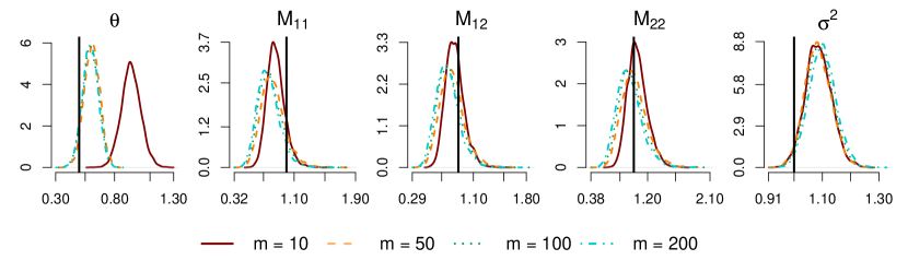
Figure S1: (Simulation study on $\mathcal{SP}(2)$). Estimated posterior distribution of $\{\theta,M,\sigma^{2}\}$ using $5\times 10^{4}$ MCMC iterations ($2\times 10^{3}$ burn-in discarded, thinned by $12$). True values are indicated by solid vertical black lines.

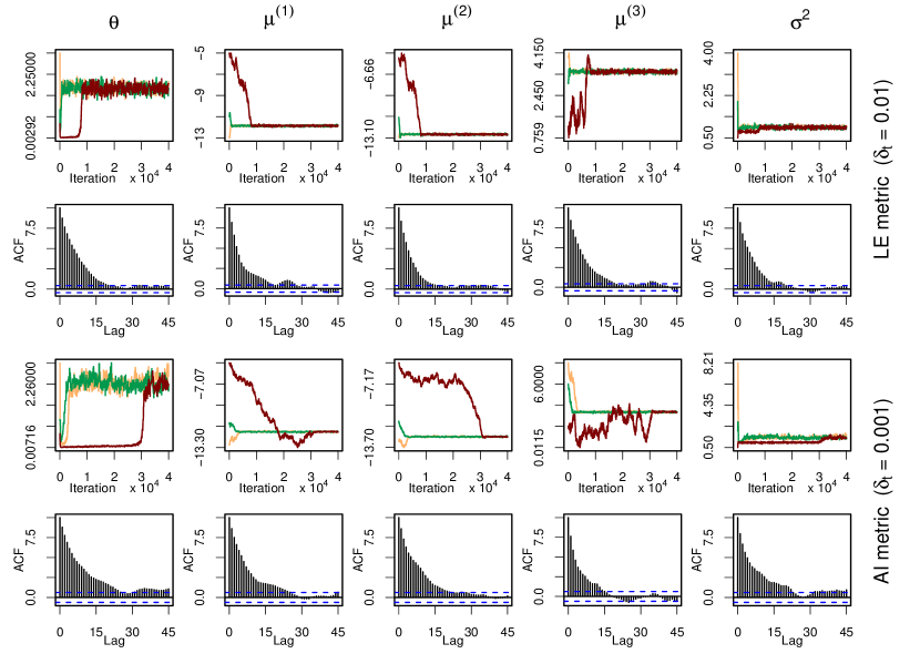
Figure S2: (Application in finance). MCMC trace plots of 4000 iterations using different starting points (orange, green and red) and ACF plots based on iterates $1000-4000$ of the green chain with $\delta_{t}=0.01$ in the case of the LE metric and $\delta_{t}=0.001$ in the case of the AI metric .

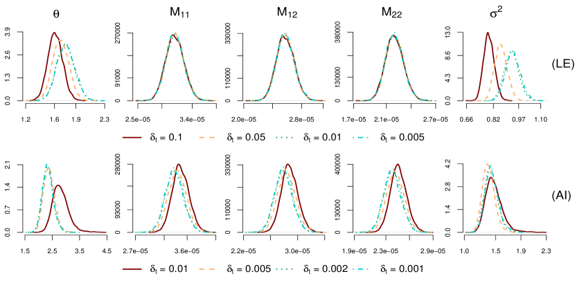
Figure S3: (Application in finance). Estimated posterior distribution for $\{\theta,M,\sigma^{2}\}$ using either the LE (top row) or the AI metric (bottom row), based on $10^{5}$ MCMC iterations ($4\times 10^{3}$ burn-in discarded, thinned by $19$).

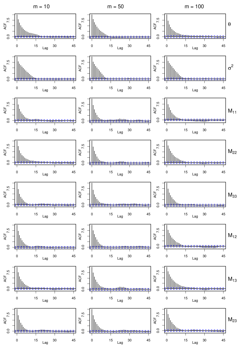
Figure S5: (Simulation study on $\mathcal{SP}(3)$). ACF plots based on iterates $10^{3}-12\times 10^{3}$ of the orange chain in Figure S4 when number of imputed points $m$ are varied over $10,\,50$ and $100$.

References

- Andersen et al. [2001a] T. G. Andersen, T. Bollerslev, F. X. Diebold, and H. Ebens. The distribution of realized stock return volatility. Journal of financial economics, 61(1):43–76, 2001a.
- Andersen et al. [2001b] T. G. Andersen, T. Bollerslev, F. X. Diebold, and P. Labys. The distribution of realized exchange rate volatility. Journal of the American statistical association, 96(453):42–55, 2001b.
- Arsigny et al. [2006] V. Arsigny, P. Fillard, X. Pennec, and N. Ayache. Log-Euclidean metrics for fast and simple calculus on diffusion tensors. Magnetic Resonance in Medicine: An Official Journal of the International Society for Magnetic Resonance in Medicine, 56(2):411–421, 2006.
- Arsigny et al. [2007] V. Arsigny, P. Fillard, X. Pennec, and N. Ayache. Geometric means in a novel vector space structure on symmetric positive-definite matrices. SIAM journal on matrix analysis and applications, 29(1):328–347, 2007.
- Asai and So [2014] M. Asai and M. K. So. Stochastic covariance models. Journal of the Japan Statistical Society, 43(2):127–162, 2014.
- Ball et al. [2008] F. G. Ball, I. L. Dryden, and M. Golalizadeh. Brownian motion and Ornstein–Uhlenbeck processes in planar shape space. Methodology and Computing in Applied Probability, 10(1):1–22, 2008.
- Barndorff-Nielsen and Shephard [2004] O. E. Barndorff-Nielsen and N. Shephard. Econometric analysis of realized covariation: High frequency based covariance, regression, and correlation in financial economics. Econometrica, 72(3):885–925, 2004.
- Barndorff-Nielsen and Stelzer [2007] O. E. Barndorff-Nielsen and R. Stelzer. Positive-definite matrix processes of finite variation. Probability and Mathematical Statistics, 27(1):3–43, 2007.
- Bauer and Vorkink [2011] G. H. Bauer and K. Vorkink. Forecasting multivariate realized stock market volatility. Journal of Econometrics, 160(1):93–101, 2011.
- Baxendale [1976] P. Baxendale. Measures and Markov processes on function spaces. Mémoires de la Société Mathématique de France, 46(131-141):3, 1976.
- Beskos et al. [2013] A. Beskos, K. Kalogeropoulos, and E. Pazos. Advanced MCMC methods for sampling on diffusion pathspace. Stochastic Processes and their Applications, 123(4):1415–1453, 2013.
- Bladt and Sørensen [2005] M. Bladt and M. Sørensen. Statistical inference for discretely observed Markov jump processes. Journal of the Royal Statistical Society: Series B (Statistical Methodology), 67(3):395–410, 2005.
- Boothby [1986] W. M. Boothby. An introduction to differentiable manifolds and Riemannian geometry, volume 120. Academic press, 1986.
- Bru [1991] M.-F. Bru. Wishart processes. Journal of Theoretical Probability, 4(4):725–751, 1991.
- Buraschi et al. [2010] A. Buraschi, P. Porchia, and F. Trojani. Correlation risk and optimal portfolio choice. The Journal of Finance, 65(1):393–420, 2010.
- Carmo [1992] M. P. d. Carmo. Riemannian geometry. Birkhäuser, 1992.
- Caseiro et al. [2012] R. Caseiro, P. Martins, J. F. Henriques, and J. Batista. A nonparametric Riemannian framework on tensor field with application to foreground segmentation. Pattern Recognition, 45(11):3997–4017, 2012.
- Chefd’Hotel et al. [2004] C. Chefd’Hotel, D. Tschumperlé, R. Deriche, and O. Faugeras. Regularizing flows for constrained matrix-valued images. Journal of Mathematical Imaging and Vision, 20(1-2):147–162, 2004.
- Chiriac and Voev [2011] R. Chiriac and V. Voev. Modelling and forecasting multivariate realized volatility. Journal of Applied Econometrics, 26(6):922–947, 2011.
- Cook et al. [2006] S. R. Cook, A. Gelman, and D. B. Rubin. Validation of software for Bayesian models using posterior quantiles. Journal of Computational and Graphical Statistics, 15(3):675–692, 2006.
- Del Moral and Murray [2015] P. Del Moral and L. M. Murray. Sequential monte carlo with highly informative observations. SIAM/ASA Journal on Uncertainty Quantification, 3(1):969–997, 2015.
- Delyon and Hu [2006] B. Delyon and Y. Hu. Simulation of conditioned diffusion and application to parameter estimation. Stochastic Processes and their Applications, 116(11):1660–1675, 2006.
- Dryden et al. [2009] I. L. Dryden, A. Koloydenko, and D. Zhou. Non-Euclidean statistics for covariance matrices, with applications to diffusion tensor imaging. The Annals of Applied Statistics, pages 1102–1123, 2009.
- Durham and Gallant [2002] G. B. Durham and A. R. Gallant. Numerical techniques for maximum likelihood estimation of continuous-time diffusion processes. Journal of Business & Economic Statistics, 20(3):297–338, 2002.
- Elerian et al. [2001] O. Elerian, S. Chib, and N. Shephard. Likelihood inference for discretely observed nonlinear diffusions. Econometrica, 69(4):959–993, 2001.
- Elworthy [1982] K. D. Elworthy. Stochastic differential equations on manifolds, volume 70. Cambridge University Press, 1982.
- Epps [1979] T. W. Epps. Comovements in stock prices in the very short run. Journal of the American Statistical Association, 74(366a):291–298, 1979.
- Eraker [2001] B. Eraker. MCMC analysis of diffusion models with application to finance. Journal of Business & Economic Statistics, 19(2):177–191, 2001.
- FirstRate Data [2019] FirstRate Data. Historical intraday index price data., 2019. http://firstratedata.com/it/index.
- Fletcher and Joshi [2007] P. T. Fletcher and S. Joshi. Riemannian geometry for the statistical analysis of diffusion tensor data. Signal Processing, 87(2):250–262, 2007.
- Gangolli [1964] R. Gangolli. On the construction of certain diffusions on a differentiable manifold. Probability Theory and Related Fields, 2(5):406–419, 1964.
- Golightly and Wilkinson [2008] A. Golightly and D. J. Wilkinson. Bayesian inference for nonlinear multivariate diffusion models observed with error. Computational Statistics & Data Analysis, 52(3):1674–1693, 2008.
- Golosnoy et al. [2012] V. Golosnoy, B. Gribisch, and R. Liesenfeld. The conditional autoregressive Wishart model for multivariate stock market volatility. Journal of Econometrics, 167(1):211–223, 2012.
- Gouriéroux [2006] C. Gouriéroux. Continuous time Wishart process for stochastic risk. Econometric Reviews, 25(2-3):177–217, 2006.
- Gouriéroux and Sufana [2010] C. Gouriéroux and R. Sufana. Derivative pricing with Wishart multivariate stochastic volatility. Journal of Business & Economic Statistics, 28(3):438–451, 2010.
- Gouriéroux et al. [2009] C. Gouriéroux, J. Jasiak, and R. Sufana. The Wishart autoregressive process of multivariate stochastic volatility. Journal of Econometrics, 150(2):167–181, 2009.
- Hansen et al. [2014] P. R. Hansen, A. Lunde, and V. Voev. Realized beta GARCH: A multivariate GARCH model with realized measures of volatility. Journal of Applied Econometrics, 29(5):774–799, 2014.
- Hong and Li [2005] Y. Hong and H. Li. Nonparametric specification testing for continuous-time models with applications to term structure of interest rates. The Review of Financial Studies, 18(1):37–84, 2005.
- Hsu [2002] E. P. Hsu. Stochastic analysis on manifolds, volume 38. American Mathematical Soc., 2002.
- Huckemann et al. [2010] S. F. Huckemann, P. T. Kim, J.-Y. Koo, and A. Munk. Möbius deconvolution on the hyperbolic plane with application to impedance density estimation. The Annals of Statistics, 38(4):2465–2498, 2010.
- Jin and Maheu [2013] X. Jin and J. M. Maheu. Modeling realized covariances and returns. Journal of Financial Econometrics, 11(2):335–369, 2013.
- Jin et al. [2019] X. Jin, J. M. Maheu, and Q. Yang. Bayesian parametric and semiparametric factor models for large realized covariance matrices. Journal of Applied Econometrics, 34(5):641–660, 2019.
- Joergensen [1978] E. Joergensen. Construction of the Brownian motion and the Ornstein-Uhlenbeck process in a Riemannian manifold on basis of the Gangolli-Mc. Kean injection scheme. Probability Theory and Related Fields, 44(1):71–87, 1978.
- Jost and Jost [2008] J. Jost and J. Jost. Riemannian geometry and geometric analysis, volume 42005. Springer, 2008.
- Jung et al. [2015] S. Jung, A. Schwartzman, and D. Groisser. Scaling-rotation distance and interpolation of symmetric positive-definite matrices. SIAM Journal on Matrix Analysis and Applications, 36(3):1180–1201, 2015.
- Kalogeropoulos et al. [2010] K. Kalogeropoulos, G. O. Roberts, and P. Dellaportas. Inference for stochastic volatility models using time change transformations. The Annals of Statistics, 38(2):784–807, 2010.
- Karcher [1977] H. Karcher. Riemannian center of mass and mollifier smoothing. Communications on pure and applied mathematics, 30(5):509–541, 1977.
- Lin et al. [2010] M. Lin, R. Chen, and P. Mykland. On generating Monte Carlo samples of continuous diffusion bridges. Journal of the American Statistical Association, 105(490):820–838, 2010.
- Lindström [2012] E. Lindström. A regularized bridge sampler for sparsely sampled diffusions. Statistics and Computing, 22(2):615–623, 2012.
- Lovett [2010] S. T. Lovett. Differential geometry of manifolds. AK Peters/CRC Press, 2010.
- Manton [2013] J. H. Manton. A primer on stochastic differential geometry for signal processing. IEEE Journal of Selected Topics in Signal Processing, 7(4):681–699, 2013.
- Matsumoto [2001] H. Matsumoto. Closed form formulae for the heat kernels and the Green functions for the Laplacians on the symmetric spaces of rank one. Bulletin des sciences mathematiques, 125(6-7):553–581, 2001.
- McKean Jr [1960] H. McKean Jr. Brownian motions on the -dimensional rotation group. Memoirs of the College of Science, University of Kyoto. Series A: Mathematics, 33(1):25–38, 1960.
- Mider et al. [2019] M. Mider, P. A. Jenkins, M. Pollock, G. O. Roberts, and M. Sørensen. Simulating bridges using confluent diffusions. arXiv preprint arXiv:1903.10184, 2019.
- Moakher [2005] M. Moakher. A differential geometric approach to the geometric mean of symmetric positive-definite matrices. SIAM Journal on Matrix Analysis and Applications, 26(3):735–747, 2005.
- Moakher and Zéraï [2011] M. Moakher and M. Zéraï. The Riemannian geometry of the space of positive-definite matrices and its application to the regularization of positive-definite matrix-valued data. Journal of Mathematical Imaging and Vision, 40(2):171–187, 2011.
- Nagano et al. [2019] Y. Nagano, S. Yamaguchi, Y. Fujita, and M. Koyama. A wrapped normal distribution on hyperbolic space for gradient-based learning. In International Conference on Machine Learning, pages 4693–4702, 2019.
- Noureldin et al. [2012] D. Noureldin, N. Shephard, and K. Sheppard. Multivariate high-frequency-based volatility (HEAVY) models. Journal of Applied Econometrics, 27(6):907–933, 2012.
- Nye [2011] T. M. Nye. Principal components analysis in the space of phylogenetic trees. The Annals of Statistics, pages 2716–2739, 2011.
- Pedersen [1995] A. R. Pedersen. Consistency and asymptotic normality of an approximate maximum likelihood estimator for discretely observed diffusion processes. Bernoulli, pages 257–279, 1995.
- Pennec [2006] X. Pennec. Statistical computing on manifolds for computational anatomy. PhD thesis, Université Nice Sophia Antipolis, 2006.
- Pennec [2020] X. Pennec. Manifold-valued image processing with SPD matrices. In Riemannian Geometric Statistics in Medical Image Analysis, pages 75–134. Elsevier, 2020.
- Pfaffel [2012] O. Pfaffel. Wishart processes. arXiv preprint arXiv:1201.3256, 2012.
- Roberts and Stramer [2001] G. O. Roberts and O. Stramer. On inference for partially observed nonlinear diffusion models using the Metropolis–Hastings algorithm. Biometrika, 88(3):603–621, 2001.
- Said et al. [2017] S. Said, L. Bombrun, Y. Berthoumieu, and J. H. Manton. Riemannian Gaussian distributions on the space of symmetric positive definite matrices. IEEE Transactions on Information Theory, 63(4):2153–2170, 2017.
- Schauer et al. [2017] M. Schauer, F. Van Der Meulen, and H. Van Zanten. Guided proposals for simulating multi-dimensional diffusion bridges. Bernoulli, 23(4A):2917–2950, 2017.
- Skovgaard [1984] L. T. Skovgaard. A Riemannian geometry of the multivariate normal model. Scandinavian Journal of Statistics, pages 211–223, 1984.
- Sommer et al. [May 2017] S. Sommer, A. Arnaudon, L. Kühnel, and S. Joshi. Bridge simulation and metric estimation on landmark manifolds. arXiv preprint arXiv:1705.10943, May 2017.
- Staneva and Younes [2017] V. Staneva and L. Younes. Learning shape trends: Parameter estimation in diffusions on shape manifolds. In Proceedings of the IEEE Conference on Computer Vision and Pattern Recognition Workshops, pages 38–46, 2017.
- Stramer et al. [2010] O. Stramer, M. Bognar, and P. Schneider. Bayesian inference for discretely sampled Markov processes with closed-form likelihood expansions. Journal of Financial Econometrics, 8(4):450–480, 2010.
- Tschumperle and Deriche [2001] D. Tschumperle and R. Deriche. Diffusion tensor regularization with constraints preservation. In Proceedings of the 2001 IEEE Computer Society Conference on Computer Vision and Pattern Recognition. CVPR 2001, volume 1, pages I–I. IEEE, 2001.
- van der Meulen and Schauer [2017] F. van der Meulen and M. Schauer. Bayesian estimation of discretely observed multi-dimensional diffusion processes using guided proposals. Electronic Journal of Statistics, 11(1):2358–2396, 2017.
- Whitaker et al. [2017] G. A. Whitaker, A. Golightly, R. J. Boys, and C. Sherlock. Improved bridge constructs for stochastic differential equations. Statistics and Computing, 27(4):885–900, 2017.
- Yu et al. [2017] P. L. Yu, W. K. Li, and F. Ng. The generalized conditional autoregressive Wishart model for multivariate realized volatility. Journal of Business & Economic Statistics, 35(4):513–527, 2017.
- Zhang [2011] L. Zhang. Estimating covariation: Epps effect, microstructure noise. Journal of Econometrics, 160(1):33–47, 2011.