Tensor spectrum of turbulence-sourced gravitational waves as a constraint on graviton mass

Abstract

We consider a generic dispersive massive gravity theory and numerically study its resulting modified energy and strain spectra of tensor gravitational waves (GWs) sourced by (i) fully developed turbulence during the electroweak phase transition (EWPT) and (ii) forced hydromagnetic turbulence during the QCD phase transition (QCDPT). The GW spectra are then computed in both spatial and temporal Fourier domains. We find, from the spatial spectra, that the slope modifications are weakly dependent on the eddy size at QCDPT, and, from the temporal spectra, that the modifications are pronounced in the $1$–$10\,{\rm nHz}$ range – the sensitivity range of the North American Nanohertz Observatory for Gravitational Waves (NANOGrav) – for a graviton mass $m_{\rm g}$ in the range $2\times 10^{-23}\,{\rm eV}\lesssim m_{\rm g}c^{2}\lesssim 7\times 10^{-22}\,{\rm eV}$.

1 Introduction

The history of gravity theories alternative to general relativity (GR) is almost as long as that of GR itself. GR propagates massless gravitons described by a linear dispersion relation $\omega=ck$, where $c$ is the speed of light. One possibility of modifying GR is by having a nonlinear dispersion relation of the form $\omega=\sqrt{c^{2}k^{2}+\omega_{\rm 0}^{2}}$, where $\omega_{\rm 0}^{2}=(m_{\rm g}c^{2}/\hbar)^{2}+\mathcal{A}c^{\alpha}k^{\alpha}$ is a frequently adopted form of a nonlinear modification [1, 2]. Here $m_{\rm g}c^{2}/\hbar$ is an effective mass term for a nonzero graviton mass $m_{\rm g}$ [3], and $\mathcal{A}$ and $\alpha$ are two Lorentz-violating parameters that do not contain $m_{\rm g}$ [1, 2]. In this paper, we focus on having an effective massive graviton term only, i.e., we only consider $\omega_{\rm cut}=m_{\rm g}c^{2}/\hbar$, and numerically studying the resulting modified gravitational wave (GW) energy spectra. However, we believe the idea of using the GW energy spectra as a constraint can be applied for a general, Lorentz-violating, modification.

So far, the graviton mass $m_{\rm g}$ has been constrained to be $m_{\rm g}\lesssim 7.7\times 10^{-23}\,{\rm eV}/c^{2}$ by LIGO [5, 4], which is already tighter than the constraint on the photon mass $m_{\gamma}\lesssim 10^{-18}\,{\rm eV}/c^{2}$ [6]. However, motivations to develop massive gravity theories remain. One such motivation is that massive gravity can explain the accelerated expansion of the universe more “naturally” than dark energy, i.e., a Yukawa-type gravitational potential of the form $\propto r^{-1}e^{-m_{\rm g}rc/\hbar}$ [8, 3, 7] arises naturally from many massive gravity theories and thus dilutes the gravitational strength at large distances without the need for a cosmological constant $\Lambda$ [9, 10]. For recent reviews, see ref. [11] on massive gravity in the context of $\Lambda$-related topics, and ref. [12] on massive gravity theories more comprehensively.

Phenomenologically, GWs offer a clean and direct constraint on the graviton mass, albeit not the tightest ones [13]. Some of the methods using GWs include orbital decay of pulsars [8], modified dispersion relation and alternative polarization modes using pulsar timing arrays [3], waveforms of extreme-mass-ratio inspirals [14] and black hole ringdowns [15], modified dispersion relation [16] and standard sirens [17] using LISA. Multi-messenger detection of GW and electromagnetic (EM) waves from binary neutron star mergers provide another direct constraint on the propagation speed difference between GW and EM waves. However, so far the bound using this method is no better than waveform measurements of GWs alone [18]; see ref. [19] on various graviton mass bounds.

Although modified GW energy spectra have been studied in the context of inflation [20], it is not well explored with a turbulent source. In particular, it is then not clear whether the spectral GW energy is enhanced or decreased in the presence of a finite graviton mass. One particular point of uncertainty arises from the fact that the equivalence between temporal and spatial spectra is now broken. In turbulence theory and numerical simulations, one computes spatial spectra, but the measurements in wind tunnels is almost always based on temporal spectra. In that case, the approximate equivalence between both spectra is accomplished by the fact that a chunk of turbulence passes by the detector at a certain mean speed $\overline{\bm{u}}$, so the fluctuations as a function of time $t$ can be translated into a spatial dependence on $\bm{x}$ through $\bm{x}=\bm{x}_{0}-\overline{\bm{u}}t$, relative to some reference point $\bm{x}_{0}$. Relic GWs, on the other hand, come from all directions, so the equivalence between spatial and temporal spectra is not that obvious—especially when there is dispersion.

Meanwhile, significant progress has been made in the numerical solution of relic GWs from turbulent sources [21, 22, 23, 24, 25]. A useful tool is the Pencil Code, a massively parallel public domain code developed by the community of users for a broad range of applications [26]. It comes with a GW solver, where the modification to dispersive GWs is straightforward. Therefore, in this work we consider turbulence-sourced GWs in a generic massive gravity theory by adding a nonzero graviton mass term $m_{\rm g}$ to the otherwise massless GW equation and explore its effect on the resulting GW spectra. Specifically, we consider GWs sourced by fully developed turbulence with an initial Kolmogorov scaling during the electroweak phase transition (EWPT) [27] and more realistic hydromagnetic turbulence that may have been present during the QCD phase transition (QCDPT) [25]. We then compute the resulting energy and strain spectra in spatial and temporal Fourier domains, which are now different due to the dispersion relation being nonlinear.

We begin by briefly recalling the basic phenomenology of massive GWs (section 2) and the relevant parameters for GWs produced during EWPTs and QCDPTs (section 3). We then present the governing equations solved in this paper (section 4), and turn then to the discussion of our results (section 5). We conclude in section 6. We use the $(-+++)$ metric signature and set $c=1$, unless specifically noted otherwise. We also normalize the critical energy density at the time of GW generation $t_{*}$ to be unity, i.e., $\rho_{\rm crit}(t_{*})=1$.

2 Massive gravity and its phenomenology

For a metric $g_{\mu\nu}=\eta_{\mu\nu}+h_{\mu\nu}$, where $\eta_{\mu\nu}=\rm diag(-+++)$ is the Minkowski background and $|h_{\mu\nu}|\ll|\eta_{\mu\nu}|$ is some small perturbation, the action of a generic massive gravity theory then can be written as

$$S=\int d^{4}x(\mathcal{L}_{\rm EH}+\mathcal{L}_{m_{\rm g}}+\mathcal{L}_{\rm mat}),$$ (2.1)

where $\mathcal{L}_{\rm EH}$ is the usual Einstein-Hilbert Lagrangian in GR, $\mathcal{L}_{m_{\rm g}}$ is a Lagrangian containing the graviton mass term $m_{\rm g}$, and $\mathcal{L}_{\rm mat}$ is a Lagrangian for matter-energy. They take the forms

$$\mathcal{L}_{\rm EH}=\sqrt{-g}R,\;\;\mathcal{L}_{m_{\rm g}}=\frac{1}{4}m_{\rm g}^{2}\sqrt{-g}\Big{(}h_{\mu\nu}h^{\mu\nu}-\frac{1}{2}h^{2}\Big{)},\;\;\mathcal{L}_{\rm mat}=-8\pi G\sqrt{-g}h^{\mu\nu}T_{\mu\nu},$$ (2.2)

where $R$ is the Ricci scalar and $T_{\mu\nu}$ is the stress-energy tensor.

Note that the modified action we are working with here is the Fierz-Pauli (FP) action [28], which is the simplest massive gravity theory. Generalizing the FP action leads to the full dRGT gravity [29, 30], for which the massive graviton term reads $\mathcal{L}_{m_{\rm g}}\propto\mathcal{U}(g,H)$, where $\mathcal{U}(g,H)$ is the sum of up to quintic order interaction terms in the perturbation metric $H_{\mu\nu}$. Conversely, the dRGT gravity reduces to FP gravity at the leading order. Therefore, since our main objective here is to deliver a qualitatively modified GW spectrum instead of the exacts of massive gravity theory, we choose the simpler FP action here.

For a conserved source, the action in equation (2.1) can be minimized by setting its variation with respect to the metric to be zero, which reads

$$0=\frac{\delta S}{\delta g^{\mu\nu}}=\int d^{4}x\sqrt{-g}\Big{(}G_{\mu\nu}+\frac{1}{2}m_{\rm g}^{2}\bar{h}_{\mu\nu}-8\pi GT_{\mu\nu}\Big{)},$$ (2.3)

where $G_{\mu\nu}\equiv R_{\mu\nu}-\frac{1}{2}g_{\mu\nu}R$ is the Einstein tensor and $\bar{h}_{\mu\nu}\equiv h_{\mu\nu}-\frac{1}{2}\eta_{\mu\nu}h$ is the trace-reversed perturbation. Keeping only the leading order terms in the perturbation $h_{\mu\nu}$ and applying the harmonic gauge $\partial^{\mu}\bar{h}_{\mu\nu}=0$, the Einstein tensor becomes

$$G_{\mu\nu}=\frac{1}{2}\Big{(}\partial_{\mu}\partial_{\rho}\bar{h}^{\rho}_{\nu}+\partial_{\nu}\partial_{\rho}\bar{h}^{\rho}_{\mu}-\partial_{\rho}\partial^{\rho}\bar{h}_{\mu\nu}-\eta_{\mu\nu}\partial_{\rho}\partial_{\sigma}\bar{h}^{\rho\sigma}\Big{)}=-\frac{1}{2}\Box\bar{h}_{\mu\nu},$$ (2.4)

where $\Box\equiv\partial_{\rho}\partial^{\rho}=-\partial_{t}^{2}+\bm{\nabla}^{2}$ is the d’Alembert operator.

Next, inserting equation (2.4) into equation (2.3) gives the linearized equation for massive gravity [8],

$$(\Box-m_{\rm g}^{2})\bar{h}_{\mu\nu}=-16\pi GT_{\mu\nu},$$ (2.5)

which is the modified GW equation. Note that we have not yet taken into account the scale factor $a$ characterizing the expansion of the universe – this will be presented in section 3. We drop the overbar of $\bar{h}_{\mu\nu}$ from here on.

In momentum space, equation (2.5) becomes

$$\ddot{h}_{\mu\nu}(\bm{k},t)+(\bm{k}^{2}+m_{\rm g}^{2})h_{\mu\nu}(\bm{k},t)=16\pi GT_{\mu\nu}(\bm{k},t),$$ (2.6)

where the double dots denote a second derivative in time, i.e., $\ddot{h}_{\mu\nu}(\bm{k},t)\equiv\partial_{t}^{2}h_{\mu\nu}(\bm{k},t)$. A direct consequence of a generic massive gravity theory is the modified dispersion relation, which now takes the form

$$\omega=\sqrt{k^{2}+\omega_{\rm cut}^{2}},$$ (2.7)

where $\omega_{\rm cut}=m_{\rm g}c^{2}/\hbar$ is an effective mass term for the graviton [3].

Another important implication of massive gravity is that the FP action given by equations (2.1) and (2.2) propagates five degrees of freedom, namely two tensor, two vector, and one scalar mode, whereas standard GR only contains two tensor modes, $+$ and $\times$. For more detailed studies on the polarization states of massive gravity, see ref. [31]. In this paper, however, we only study the spectral modifications of the tensor mode for the following reasons. First, detection of any extra polarization modes would automatically indicate a modified gravity theory, whereas modifications of the tensor modes that are also present in GR are more subtle to discern. Second, although the construction is different from the FP gravity here, there exists a Lorentz-violating minimal theory of massive gravity (MTMG) that only carries two tensor modes of GWs [32, 33]. These highlight the significance of studying tensor GWs separately. And third, the nonlinear dispersion in equation (2.7) holds for all modes, which means the spectral modifications of tensor modes should have qualitatively valid features for additional modes, too. However, perhaps for a future project, it is also important to investigate the extra polarization modes in the context of low-frequency GWs, since below around $10^{-7}\,{\rm Hz}$, these modes can have amplitudes similar to those of the tensor modes in GR [34].

3 Tensor mode gravitational waves from the early universe

Equation (2.5) gives the linearized equation for massive gravity. For the early universe, we adopt the normalization such that the scale factor at the time of GW generation, $t_{*}$, is set to be unity, i.e., $a_{*}\equiv a(t_{*})=1$. The Hubble parameter at that time is $H_{\ast}$, defined to be $H_{*}=\sqrt{8\pi G\rho_{\rm crit}(t_{*})/3}$, where $\rho_{\rm crit}(t_{*})$ is the critical energy density at time $t_{*}$. We denote $\omega_{0}^{H}=2\pi H_{*}/a_{0}$ as the Hubble frequency scaled to the present, $m_{\rm g}^{H}=\hbar\omega_{0}^{H}$ as the graviton mass corresponding to the Hubble frequency and $\lambdabar_{0}^{H}=1/\omega_{0}^{H}$ as the reduced Compton wavelength of such a graviton scaled to the present.

Furthermore, we assume an adiabatic expansion of the universe during the radiation-dominated era. This means $g_{S}(T)\,T^{3}a^{3}(T)$ stays constant by entropy conservation, where $g_{S}(T)$ is the number of adiabatic degrees of freedom at temperature $T$. Using $T_{*}^{\rm EW}\approx 100\,{\rm GeV}$ and $g_{S}(T_{*}^{\rm EW})\approx 100$ at EWPT, $T_{*}^{\rm QCD}\approx 150\,{\rm MeV}$ and $g_{S}(T_{*}^{\rm QCD})\approx 15$ at QCDPT, combined with $T_{0}=2.7\,{\rm K}$ and $g_{S}(T_{0})=3.9$ at the present, we obtain $a_{0}/a_{*}^{\rm EW}\sim 1.3\times 10^{15}$ and $a_{0}/a_{*}^{\rm QCD}\sim 10^{12}$.

To obtain the Hubble parameter, we need the critical energy density in physical units. During the radiation era, the critical energy density of the universe is approximately the radiation energy density, i.e., $\rho_{\rm crit}(t_{*})\simeq\mathcal{E}_{\rm rad}(t_{*})=\pi^{2}g_{S}(T_{*})k_{B}^{4}T_{*}^{4}/(30\hbar^{3}c^{3})$, where $k_{\rm B}$ is the Boltzmann constant. We note that, in agreement with some earlier work [23, 24, 25], we use now the symbol $\mathcal{E}$ for mean energy densities, but keep the commonly used symbol $\rho$ for the critical density, which includes the rest mass density.

For EWPT and QCDPT, we get $H_{*}^{\rm EW}\approx 2.1\times 10^{10}\rm s^{-1}$ and $H_{*}^{\rm QCD}\approx 1.8\times 10^{4}\rm s^{-1}$, respectively. Given $H_{0}\approx 3.2\times 10^{-18}\rm s^{-1}$ today, we obtain $H_{0}/H_{*}^{\rm EW}\approx 1.5\times 10^{-28}$ and $H_{0}/H_{*}^{\rm QCD}\approx 1.8\times 10^{-22}$. Using these, we can obtain the energy dilution factor $(a_{*}/a_{0})^{4}(H_{*}/H_{0})^{2}$, which we should multiply the generated energy by in order to obtain its present day value in the form $h_{0}^{2}\Omega_{\rm GW}$ [21, 22], which is independent of the uncertainty in the normalized present day Hubble parameter $h_{0}\approx 0.7$. Table 1 summarizes the aforementioned scaling factors, together with some useful parameters for EWPT and QCDPT.

We adopt the conformal scaling such that $h_{\mu\nu}=ah_{\mu\nu}^{\rm phys}$ and $T_{\mu\nu}^{\rm TT}=a^{4}T_{\mu\nu,{\rm phys}}^{\rm TT}$, and the relation $a(t)\propto t$ during the radiation dominated era, so the GW equation (2.5) becomes

$$\Big{(}\partial_{t}^{2}+m_{\rm g}^{2}-\bm{\nabla}^{2}\Big{)}h_{\mu\nu}=\frac{16\pi G}{a}T_{\mu\nu}^{\rm TT},$$ (3.1)

where the superscript TT denotes the transverse-traceless (TT) projection. We solve this equation in Fourier space and work with the stress projected onto the linear polarization basis, where $+$ and $\times$ denote the plus and cross polarizations; see [35, 36] for details and [21] for the implementation in the Pencil Code.

Using normalized conformal time $\bar{t}=t/t_{*}$, scaled wave vector $\bar{\bm{k}}=\bm{k}/H_{*}$, and scaled normalized stress $\bar{T}^{\rm TT}_{+/\times}=T^{\rm TT}_{+/\times}/\mathcal{E}_{\rm rad}^{*}$, the GW equation in momentum space (equation (2.6)) becomes

$$\Big{(}\partial_{\bar{t}}^{2}+m_{\rm g}^{2}+\bar{\bm{k}}^{2}\Big{)}h_{+/\times}(\bm{k},t)=\frac{6}{\bar{t}}\,\bar{T}^{\rm TT}_{+/\times}(\bm{k},t),$$ (3.2)

but we will drop the overbars from now on, except for one case where we explicitly compare with $\bm{x}$ and $t$ in physical space. Note that this is modified upon equation (13) in ref. [21].

Finally, in terms of observables, we define the characteristic strain amplitude as $h_{\rm rms}=\langle h^{2}\rangle^{1/2}$, where $h^{2}\equiv h_{+}^{2}+h_{\times}^{2}=h_{\mu\nu}^{2}/2$, as well as the scaled GW energy $\mathcal{E}_{\rm GW}=\langle\dot{h}^{2}\rangle/6$, where $\dot{h}^{2}=\dot{h}_{+}+\dot{h}_{\times}$ and $\dot{h}_{+/\times}=\partial_{t}h_{+/\times}$, but see ref. [21] for a small correction term that will here be neglected.

Event	$k_{\rm B}T$	$\omega_{0}^{H}[\rm Hz]$	$m_{\rm g}^{H}[\,{\rm eV}/c^{2}]$	$\lambdabar_{0}^{H}[\rm m]$	$(a_{*}/a_{0})^{4}(H_{*}/H_{0})^{2}$
EWPT	$100\,{\rm GeV}$	$1.0\times 10^{-4}$	$6.8\times 10^{-20}$	$1.9\times 10^{13}$	$1.6\times 10^{-5}$
QCDPT	$150\,{\rm MeV}$	$1.1\times 10^{-7}$	$7.4\times 10^{-23}$	$1.7\times 10^{16}$	$3.1\times 10^{-5}$

Table 1: Scaling factors and useful parameters.

4 Hydromagnetic turbulent sources

The full set of governing equations for the density $\rho$, velocity field $\bm{u}$, and magnetic field $\bm{B}$ with $\bm{\nabla}\cdot\bm{B}=0$ in conformal time and comoving variables [37, 27] are

$$\frac{\partial\ln\rho}{\partial t}= -\frac{4}{3}(\bm{\nabla}\cdot\bm{u}+\bm{u}\cdot\bm{\nabla}\ln\rho)+\frac{1}{\rho}[\bm{u}\cdot(\bm{J}\cdot\bm{B})+\eta\bm{J}^{2}]$$ (4.1)

$$\begin{split}\frac{D\bm{u}}{Dt}=&\frac{\bm{u}}{3}(\bm{\nabla}\cdot\bm{u}+\bm{u}\cdot\bm{\nabla}\ln\rho)-\frac{\bm{u}}{\rho}[\bm{u}\cdot(\bm{J}\times\bm{B})+\eta\bm{J}^{2}]\\ &-\frac{1}{4}\bm{\nabla}\ln\rho+\frac{3}{4\rho}\bm{J}\times\bm{B}+\frac{2}{\rho}\bm{\nabla}\cdot(\rho\nu\bm{\mathsf{S}})\end{split}$$ (4.2)

$$\frac{\partial\bm{B}}{\partial t}= \bm{\nabla}\times(\bm{u}\times\bm{B}-\eta\bm{J}+\bm{\mathcal{F}}),$$ (4.3)

where $\bm{J}=\bm{\nabla}\times\bm{B}$ is the magnetic current, $D/Dt=\partial/\partial t+\bm{u}\cdot\bm{\nabla}$ is the advective derivative, $\nu$ is the kinematic viscosity, $\eta$ is the magnetic diffusivity, and $\mathsf{S}_{ij}=\frac{1}{2}(u_{i,j}+u_{j,i})-\frac{1}{3}\delta_{ij}u_{k,k}$ are the components of the traceless strain tensor $\bm{\mathsf{S}}$.

For the EWPT, we start with a turbulence spectrum that has Kolmogorov scaling in $k$ space, i.e., the initial condition of the evolving turbulence considered in ref. [27]. We have a magnetic field of the form

$$\bm{B}_{i}(\bm{k})=\bm{B}_{*}[P_{ij}(\bm{k})-i\sigma_{\rm M}\epsilon_{ijl}\hat{k}_{l}]g_{j}(\bm{k})S(k),$$ (4.4)

where $P_{ij}=\delta_{ij}-\hat{k}_{i}\hat{k}_{j}$ is the projection operator, $\sigma_{\rm M}$ indicates helicity and is set to 1 in our runs, $\epsilon_{ijl}$ is the Levi-Civita symbol, $g_{j}(\bm{k})$ is the Fourier transform of a random $\delta$-correlated vector field with Gaussian fluctuations, i.e., $g_{i}(\bm{x})g_{j}(\bm{x}^{\prime})=\delta_{ij}\delta^{3}(\bm{x}-\bm{x}^{\prime})$, and $S(k)$ determines the spectral shape with

$$S(k)=\frac{k_{\rm f}^{-3/2}(k/k_{\rm f})^{\alpha/2-1}}{[1+(k/k_{\rm f})^{2(\alpha+5/3)}]^{1/4}},$$ (4.5)

where $k_{\rm f}$ is the wave number of the energy-carrying eddies and $\alpha=4$ for a causal spectrum, such that $S(k)\sim k$ for small $k$ and $S(k)\sim k^{-5/3}$ for large $k$.

For QCDPT, we start with zero magnetic field and, as in ref. [25], apply instead a forcing function $\bm{\mathcal{F}}$ with

$$\bm{\mathcal{F}}(\bm{x},t)={\rm Re}[\mathcal{N}\tilde{\bm{f}}(\bm{k})\exp(i\bm{k}\cdot\bm{x}+i\varphi)],$$ (4.6)

where the wave vector $\bm{k}(t)$ and the phase $\varphi(t)$ change randomly at each time step. This forcing function is therefore white noise in time and consists of plane waves with average wave number $k_{\rm f}$ such that $|\bm{k}|$ lies in an interval $k_{\rm f}-\delta k/2\leq|\bm{k}|<k_{\rm f}+\delta k/2$ of width $\delta k$. $\mathcal{N}={\cal F}_{0}/\delta t^{1/2}$ is a normalization factor, where $\delta t$ is the time step and ${\cal F}_{0}$ is varied to achieve a certain magnetic field strength after a certain time, and $\tilde{\mathcal{F}}(\bm{k})=(\bm{k}\times\bm{e})/[\bm{k}^{2}-(\bm{k}\cdot\bm{e})^{2}]^{1/2}$ is a nonhelical forcing function. Here $\bm{e}$ is an arbitrary unit vector that is not aligned with $\bm{k}$. Note that $|\mathcal{F}|^{2}=1$. As in ref. [25], this forcing is only enabled during the time interval $1\leq t\leq 2$. The kinetic and magnetic energy densities are defined as $\mathcal{E}_{\rm K}(t)=\langle\rho\bm{u}^{2}\rangle/2$ and $\mathcal{E}_{\rm M}(t)=\langle\bm{B}^{2}\rangle/2$.

5 Energy spectra from numerical simulations

We use the Pencil Code [26] to solve equation (3.2) together with a forced magnetic field given by equations (4.4) and (4.5) at EWPT, and together with equations (4.1)–(4.3) for turbulence at QCDPT. The runs discussed in this paper are summarized in table 2. The numerical data for our spectra are publicly available [38]. We recall that in the code, our nondimensional wave numbers and frequencies correspond, at the present time, to $1/\lambdabar_{0}^{H}$ and $\omega_{0}^{H}$, respectively. The numerical resolution for the runs is arranged as follows: all EWPT runs (E1 through F5) have $1152^{3}$ mesh points each, except for F1, which has $1024^{3}$ points; and all QCDPT runs (Q1 through P5) have $512^{3}$ mesh points. We also set $\nu=\eta=5\times 10^{-5}$ for all runs. In table 2 we list four groups of runs: two that are applied to the EWPT (E1–E4 with $\mathcal{E}_{\rm M}=7.8\times 10^{-3}$ and F1–F5 with $\mathcal{E}_{\rm M}=5.6\times 10^{-3}$) and two that are applied to the QCDPT (Q1–Q4 with $\mathcal{E}_{\rm M}=3.9\times 10^{-2}$ and P1–P5 with $\mathcal{E}_{\rm M}=3.8\times 10^{-2}$). For each group, we vary the value of $\omega_{\rm cut}$, which does not affect the values of $\mathcal{E}_{\rm M}$, which are therefore not listed in table 2.

Runs	$k_{1}$	$k_{\rm f}$	$\omega_{\rm cut}$	$\mathcal{E}_{\rm GW}^{\rm sat}$	$h_{\rm rms}^{\rm sat}$	$h_{0}^{2}\Omega_{\rm GW}$	$h_{\rm c}$
E1	$100$	$600$	0	$1.15\times 10^{-10}$	$9.36\times 10^{-8}$	$1.89\times 10^{-15}$	$7.46\times 10^{-23}$
E2	$100$	$600$	10	$1.13\times 10^{-10}$	$1.15\times 10^{-7}$	$1.85\times 10^{-15}$	$9.19\times 10^{-23}$
E3	$100$	$600$	50	$1.12\times 10^{-10}$	$9.95\times 10^{-8}$	$1.85\times 10^{-15}$	$7.93\times 10^{-23}$
E4	$100$	$600$	200	$1.03\times 10^{-10}$	$6.44\times 10^{-8}$	$1.69\times 10^{-15}$	$5.13\times 10^{-23}$
F1	$1$	$100$	0	$3.77\times 10^{-9}$	$8.93\times 10^{-6}$	$6.20\times 10^{-14}$	$7.12\times 10^{-21}$
F2	$1$	$100$	0.3	$3.84\times 10^{-9}$	$8.34\times 10^{-6}$	$6.31\times 10^{-14}$	$6.65\times 10^{-21}$
F3	$1$	$100$	1	$3.83\times 10^{-9}$	$7.06\times 10^{-6}$	$6.29\times 10^{-14}$	$5.63\times 10^{-21}$
F4	$1$	$100$	3	$3.74\times 10^{-9}$	$3.91\times 10^{-6}$	$6.14\times 10^{-14}$	$3.12\times 10^{-21}$
F5	$1$	$100$	10	$3.68\times 10^{-9}$	$2.01\times 10^{-6}$	$6.06\times 10^{-14}$	$1.60\times 10^{-21}$
Q1	0.3	2	0	$4.86\times 10^{-4}$	$4.16\times 10^{-2}$	$1.50\times 10^{-8}$	$4.17\times 10^{-14}$
Q2	0.3	2	0.3	$4.70\times 10^{-4}$	$3.44\times 10^{-2}$	$1.45\times 10^{-8}$	$3.44\times 10^{-14}$
Q3	0.3	2	1	$3.91\times 10^{-4}$	$2.05\times 10^{-2}$	$1.21\times 10^{-8}$	$2.06\times 10^{-14}$
Q4	0.3	2	3	$1.99\times 10^{-4}$	$8.48\times 10^{-3}$	$6.15\times 10^{-9}$	$8.49\times 10^{-15}$
Q5	0.3	2	10	$3.41\times 10^{-5}$	$1.37\times 10^{-3}$	$1.05\times 10^{-9}$	$1.37\times 10^{-15}$
P1	1	6	0	$5.05\times 10^{-5}$	$4.62\times 10^{-3}$	$1.56\times 10^{-9}$	$4.63\times 10^{-15}$
P2	1	6	0.3	$5.02\times 10^{-5}$	$4.48\times 10^{-3}$	$1.55\times 10^{-9}$	$4.48\times 10^{-15}$
P3	1	6	1	$4.81\times 10^{-5}$	$3.54\times 10^{-3}$	$1.49\times 10^{-9}$	$3.55\times 10^{-15}$
P4	1	6	3	$3.97\times 10^{-5}$	$2.07\times 10^{-3}$	$1.23\times 10^{-9}$	$2.08\times 10^{-15}$
P5	1	6	10	$1.85\times 10^{-5}$	$7.71\times 10^{-4}$	$5.72\times 10^{-10}$	$7.71\times 10^{-16}$

Table 2: Summary of runs shown in the paper. $k_{1}$ is the smallest wave number in the simulation domain, and $k_{\rm f}$ characterizes the peak magnetic energy. $h_{0}^{2}\Omega_{\rm GW}$ and $h_{\rm c}$ are the values of $\mathcal{E}_{\rm GW}^{\rm sat}$ and $h_{\rm rms}^{\rm sat}$ scaled to the present day, respectively.

5.1 Spatial Fourier spectra

Following ref. [21], we define spatial Fourier spectra as integrals over concentric shells in wave number space (indicated now by a single tilde), i.e.,

$${\rm Sp}_{k}(h)=\int_{4\pi}\left[\left|\tilde{h}_{+}(\bm{k},t)\right|^{2}+\left|\tilde{h}_{\times}(\bm{k},t)\right|^{2}\right]k^{2}\,{\rm d}\Omega_{k},$$ (5.1)

where ${\rm d}\Omega_{k}$ is the differential over the solid angle in $\bm{k}$ space. An analogous definition applies also to $\dot{h}$, which is used for calculating $E_{\rm GW}(k,t)={\rm Sp}_{k}(\dot{h})/6$, but see equation (B.36) of ref. [21] for lower order correction terms that are here neglected.

For EWPT, we first choose the same parameters as in ref. [22], where the smallest wave number in the simulation domain is $k_{1}=100$ and the peak wave number is $k_{\rm f}=600$. The resulting GW energy density today, $h_{0}^{2}\Omega_{\rm GW}(k)$, and the strain today, $h_{\rm c}(k)$, as functions of wave number $k$ are shown in figure 1(a). We see that for all the effective mass terms $\omega_{\rm cut}\in\{10,50,200\}$ corresponding to $m_{\rm g}\in\{6.8\times 10^{-19},3.4\times 10^{-18},1.4\times 10^{-17}\}\,{\rm eV}/c^{2}$, the spectral modifications are not significant, even though $\omega_{\rm cut}=200$ already corresponds to an unrealistically large graviton mass $m_{\rm g}=1.4\times 10^{-17}\,{\rm eV}/c^{2}$.

Next, we explore the same EWPT era but with $k_{1}=1$ and $k_{\rm f}=100$, and the effective mass term $\omega_{\rm cut}\in\{0.3,1,3,10\}$, corresponding to a range of graviton masses $m_{\rm g}\in\{2.0\times 10^{-20},6.8\times 10^{-20},2.0\times 10^{-19},6.8\times 10^{-19}\}\,{\rm eV}/c^{2}$. The resulting spectra are shown in figure 1(b). Now the spectral differences are more significant than before, especially towards the lower wave number at around $k_{1}$. For the spectral energy density $h_{0}^{2}\Omega_{\rm GW}(k)$, the left panel of figure 1(b) shows spectral shape changes by about a factor of $k^{1.2}$, from $k^{6/5}$ to $k^{12/5}$. For the strain $h_{\rm c}(k)$, the right-hand panel of figure 1(b) shows slope changes correspondingly by about a factor $k^{1.6}$, from $k^{-2/5}$ to $k^{6/5}$ as we increase the graviton mass. However, the constraint on the graviton mass provided by GWs from EWPT is not significant overall, as can be seen from table 1, compared to the existing constraint of $m_{\rm g}\lesssim 7.7\times 10^{-23}\,{\rm eV}/c^{2}$ [5, 4] that we quoted in the introduction.

Since the QCDPT era could provide a constraint on the graviton mass tighter than EWPT by about three orders of magnitude (table 1), we would like to explore the spectral behaviors of GWs from the QCDPT era. For this we adopt the simulation setup of previous work [25], since the only change here is adding an effective graviton mass term $\omega_{\rm cut}$. We have two series of runs, the first with $k_{1}=0.3$ and $k_{\rm f}=2$ (runs Q2 to Q5), and the second with $k_{1}=1$ and $k_{\rm f}=6$ (runs P2 to P5). For both series, we vary $\omega_{\rm cut}\in\{0.3,1,3,10\}$, corresponding to a range of graviton masses $m_{\rm g}\in\{2.2\times 10^{-23},7.4\times 10^{-23},2.2\times 10^{-22},7.4\times 10^{-22}\}\,{\rm eV}/c^{2}$. The resulting energy and strain spectra can be seen in figures 1(c) and 1(d), which show remarkably consistent modifications for the two series. We see that for both cases, as the graviton mass increases, the spectral shapes at lower wave numbers, around the corresponding value of $k_{1}$, become steeper. In particular, figure 1(c) shows that for $k_{\rm f}=2$, the energy density $h_{0}^{2}\Omega_{\rm GW}$ goes from $k^{8/5}$ to $k^{3}$, and the strain $h_{\rm c}$ goes from $k^{-1/5}$ to $k^{3/2}$; and figure 1(d) shows that for $k_{\rm f}=6$, the energy density changes from $k^{1}$ to $k^{3}$, and the strain from $k^{-1/2}$ to $k^{3/2}$, respectively. Therefore, the spectral modifications are only weakly dependent on the driving wave number.

Note that in figures 1(a)–d, we observe the expected slope correspondence between GW energy density and strain, i.e., in the small graviton mass limit, we have $h_{0}^{2}\Omega_{\rm GW}(k)\propto k^{2}h_{c}^{2}(k)$, and in the large graviton mass limit, the relation changes to $h_{0}^{2}\Omega_{\rm GW}(k)\propto h_{c}^{2}(k)$.

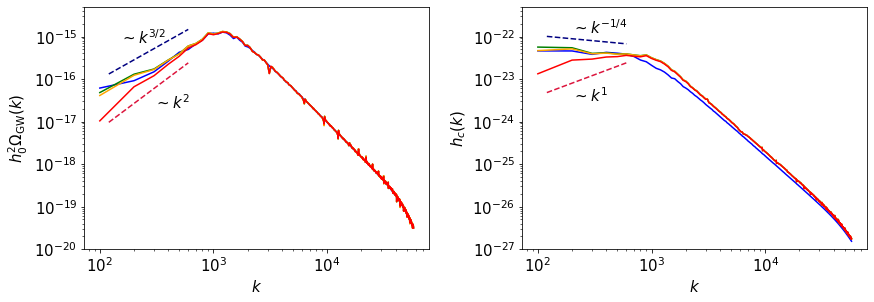
(a) Runs E1 to E4: $\omega_{\rm cut}=0$ (blue), 10 (green), 50 (orange), and 200 (red).

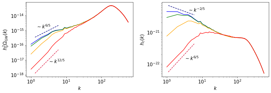
(b) Runs F2 to F5: $\omega_{\rm cut}=0.3$ (blue), 1 (green), 3 (orange), and 10 (red).

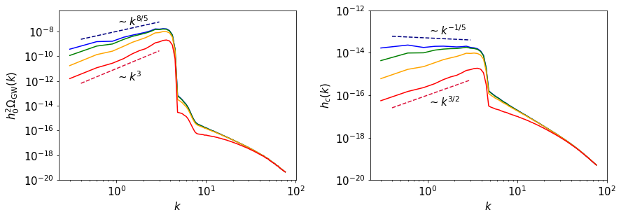
(c) Runs Q2 to Q5: $\omega_{\rm cut}=0.3$ (blue), 1 (green), 3 (orange), and 10 (red).

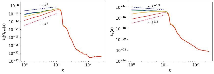
(d) Runs P2 to P5: $\omega_{\rm cut}=0.3$ (blue), 1 (green), 3 (orange), and 10 (red).

Figure 1: Spectra of GW energy density $h_{0}^{2}\Omega_{\rm GW}(k)$ and strain $h_{\rm c}(k)$ from EWPT and QCDPT scaled to the present time.

To understand the systematic change from $h_{0}^{2}\Omega_{\rm GW}(k)\propto k^{3}$ to $h_{\rm c}(k)\propto k^{3/2}$ in the QCD runs, it is important to recall that for a causal spectrum of the magnetic field with ${\rm Sp}(\bm{B})\propto k^{4}$ [39], the stress only has a spectrum proportion to $k^{2}$ [40]. This is because a blue spectrum convolved with itself can only become white noise. It implies that ${\rm Sp}([k^{2}+\omega_{\rm cut}^{2}]h)\propto k^{2}$, and therefore

$$h_{\rm c}=\sqrt{k\,{\rm Sp}(h)}\propto k^{3/2}/(k^{2}+\omega_{\rm cut}^{2})\propto k^{3/2}$$ (5.2)

for $k\ll\omega_{\rm cut}$. The spectrum of $\dot{h}$, on the other hand, is given by $\omega^{2}{\rm Sp}(h)\propto k^{2}/(k^{2}+\omega_{\rm cut}^{2})$, and therefore

$$h_{0}^{2}\Omega_{\rm GW}(k)=k\,{\rm Sp}({\dot{h})}\propto k^{3}/(k^{2}+\omega_{\rm cut}^{2})\propto k^{3}$$ (5.3)

for $k\ll\omega_{\rm cut}$. These considerations clearly demonstrate the obtained trend in figures 1(c) and 1(d) from the $h_{0}^{2}\Omega_{\rm GW}(k)\propto k^{3}$ scaling to a $h_{\rm c}(k)\propto k^{3/2}$ scaling. We also see that, relative to the case $\omega_{\rm cut}=0$, both spectra decrease in amplitude by a factor $1/\omega_{\rm cut}^{2}$. This is well borne out by the simulations, where we see a drop by $1/100$ in both panels of figure 1(b) for $\omega_{\rm cut}=10$.

For all the graviton masses considered, the patterns at higher wave numbers are approximately the same, including a sharp drop by many orders of magnitude found previously in the massless case discussed in ref. [25]. We return to this feature further below.

In order to make closer connections to potential detections, we would like to inspect the temporal Fourier spectra next. In particular, we will show that both EWPT and QCDPT could induce observable features in the $\sim 10\,{\rm nHz}$ range, accessible by NANOGrav.

5.2 Temporal Fourier spectra

As alluded to in the introduction, spatial and temporal spectra can be different from each other if there is nonlinear dispersion. To the best of our knowledge, it is the first time that GW spectra have been obtained from turbulence simulations in terms of temporal frequency. To compute temporal spectra, we first Fourier transform $\tilde{h}_{+}(\bm{k},t)$ and $\tilde{h}_{\times}(\bm{k},t)$ back into real space to obtain time series

$$h_{+/\times}(\bm{x},t)=\int\tilde{h}_{+/\times}(\bm{k},t)\,e^{{\rm i}\bm{k}\cdot\bm{x}}\,{\rm d}^{3}\bm{k}/(2\pi)^{3}.$$ (5.4)

We then compute their Fourier transforms to $\omega$ space as $\tilde{\tilde{h}}_{+/\times}(\bm{x},\omega)=\int h_{+/\times}(\bm{x},t)\,e^{{\rm i}\omega t}\,{\rm d}t$ at several points $\bm{x}_{i}$. We finally compute the mean spectrum as

$${\rm Sp}_{\omega}(h)=N^{-1}\sum_{i=1}^{N}\left[\left|\tilde{\tilde{h}}_{+}(\bm{x}_{i},\omega)\right|^{2}+\left|\tilde{\tilde{h}}_{\times}(\bm{x}_{i},\omega)\right|^{2}\right],$$ (5.5)

which is an average over $N$ spatial points. In practice, we take $N=1024$, which is the number of mesh points of the simulations in the $x$ direction. The results for ${\rm Sp}_{\omega}(h)$ are shown in figure 2, where we also compare with ${\rm Sp}_{k}(h)$ using both $\omega=k$ (ignoring dispersion, which is only valid for $\omega_{\rm cut}=0$) and $\omega=\sqrt{k^{2}+\omega_{\rm cut}^{2}}$ (valid also in the presence of dispersion, with $\omega_{\rm cut}\neq 0$). Since

$$\int{\rm Sp}_{\omega}(h)\,{\rm d}\omega=\int{\rm Sp}_{k}(h)\,{\rm d}k=h_{\rm rms}^{2},$$ (5.6)

we present in the following $(\omega/k)\,{\rm Sp}_{k(\omega)}(h)$, where the factor ${\rm d}k/{\rm d}\omega=\omega/k$ (for $\omega>\omega_{\rm cut}$) has been applied to take the effect of dispersion into account.

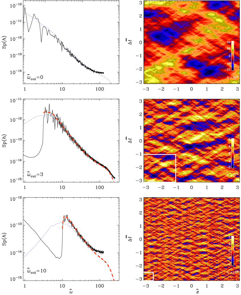
Figure 2: Left: temporal strain spectra (solid lines) compared with spatial strain spectra with (red dashed lines) and without (blue dotted lines) the transformation to $\omega$ space applied, for $\omega_{\rm cut}=0$, 3, and 10. Right: space–time diagrams of the strain for runs F1, F4, and F5 with $\omega_{\rm cut}=0$, 3, and 10. The small white boxes on the lower left corner of the last two strain diagrams with a size of $2\pi/\omega_{\rm cut}$ are given for orientation. The color bars give the present-day physical strain multiplied by $10^{18}$.

In figure 2, we also show contour plots of $h(\bm{x},t)$ through an arbitrarily selected section $\bm{x}=(x,0,0)$ for the same three cases with $\omega_{\rm cut}=0$, 3, and 10. They would give us a direct impression of how the GW field would vary in the proximity of the Sun in space and time.

The temporal spectra show a sharp drop near $\omega=\omega_{\rm cut}$, but ${\rm Sp}_{\omega}(h)$ only drops by about two orders of magnitude and does not vanish completely. Moreover, towards smaller values of $\omega<\omega_{\rm cut}$, ${\rm Sp}_{\omega}(h)$ begins to rise again. This is probably just a consequence of having a finite length of the time series, which makes the statistical error large at small frequencies.

The drop in spectral power below $\omega_{\rm cut}$ also has marked consequences for the appearance of $h(x,t)$ in real space (right-hand panels of figure 2, which show smaller scale patches in space and time whose size is comparable to $2\pi/\omega_{\rm cut}$ in space, but only about half as long as $2\pi/\omega_{\rm cut}$ in time. For $\omega_{\rm cut}=0$, on the other hand, we see extended patches in $h(x,t)$ that are all comparable in size to the scale of the domain. We note at this point that in all three plots of $h(x,t)$, we have selected a time interval of the length $2\pi$, i.e., the same interval as in $x$. We select the time interval to be near the end of the run, but other time intervals look similar.

On the outer axes of figure 2, we have indicated the values scaled to a physical time corresponding to the QCDPT, using $t=(a_{0}/H_{\ast})\,\bar{t}$ and $x=(ca_{0}/H_{\ast})\,\bar{x}$ with $a_{0}=10^{12}$, $H_{\ast}=1.8\times 10^{4}\,{\rm s}^{-1}$, $c=3\times 10^{8}\,{\rm m}\,{\rm s}^{-1}$ being the physical dimensions used. We see that the patches can become as short as a fraction of a year.

In figure 3, we show ${\rm Sp}_{\omega}(h)$ and contour plots of $h(\bm{x},t)$ for runs Q1 and Q3 with $\omega_{\rm cut}=0$ and 1. One of the major features in the runs shown in figure 2 is the presence of a sharp drop of spectral power for wave numbers above $2k_{\rm f}\approx 6$. This translates to a similar drop also in the $\omega$ spectra, but now, when $\omega_{\rm cut}=1$, GWs exist only over a narrow range of frequencies. This is probably also the reason why the space–time diagrams of the strain show a somewhat more regular pattern for $\omega_{\rm cut}=1$.

Finally, we note that in figure 3 between $\omega\sim 10$ and $\omega\sim 100$, the blue dotted lines sharply drop by several orders of magnitude, exposing a divergence between the black solid lines. This disagreement between the $\omega$ and $\bm{k}$ spectra is not related to the graviton mass, but it is primarily related to the sharp drop in ${\rm Sp}(h)$ above $\bar{\omega}=k_{\rm f}=3$. We have seen such a drop in runs with low $k_{\rm f}$ for the QCD runs (figures 1(c) and 1(d)). One might think that it could be related to the Reynolds number not being large enough. However, we have been able to increase the Reynolds number by a factor of ten and have still not seen any significant change in this drop. On the other hand, temporal spectra are not as accurate as spatial ones, which take the entire data cube into account. They are therefore more easily affected by statistical noise. Given that the drop extends over several orders of magnitude, the differences between the spatial and temporal spectra occur where the spatial spectrum is already very weak and below the noise level of the temporal spectrum. Note that this feature of a sharp drop is also present in a physically more realistic turbulence source driven by inflationary magnetogenesis [41]. The weak temporal signal beyond this drop is therefore most likely no longer reliable.

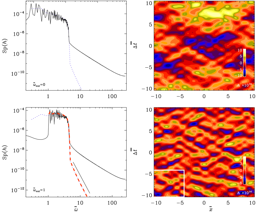
Figure 3: Similar to figure 2, but for runs Q1 and Q3 with $\omega_{\rm cut}=0$ and 1, respectively. The color bars give the physical strain multiplied by $10^{14}$.

6 Discussions and conclusions

We have seen that, depending on different values of graviton masses considered, GW energy and strain can exhibit significant modifications, mainly in terms of spectral shapes. The spectra of relic GWs from EWPT and QCDPT have the potential to constrain the graviton mass and, in turn, massive gravity theories. For GWs from fully developed hydromagnetic turbulence at EWPT, the spectral changes are not so pronounced when $k_{\rm f}=600$ and $k_{1}=100$, but become more significant when $k_{\rm f}=100$ and $k_{1}=1$, allowing us to see changes at low wave numbers near $k_{1}$. Specifically, the changes here are that the energy and strain spectra both become steeper by slightly more than a $k^{1}$ factor as we increase the graviton mass by about 30 fold. For QCDPT, we see that GWs induced by forced hydromagnetic turbulence also exhibit steepening spectral slopes around $k_{1}$ by up to a $k^{2}$ factor as the graviton mass increases by about 30 fold. Quite remarkably, the spectral slopes are only weakly affected by different driving wave numbers, meaning that, even if we are unsure about the exact number of turbulent eddies at the time of QCDPT, we could still use the GW spectra to constrain the graviton mass. For both EWPT and QCDPT, the relic GW energy in the low wave number tails is expected to be lower in the presence of a nonzero graviton mass, although the values at high wave numbers are roughly unchanged.

The frequency spectra can directly be obtained from wave number spectra through a simple transformation, which takes $\omega_{\rm cut}\neq 0$ into account. Our work has demonstrated that the agreement between both types of spectra is rather good, but frequency spectra obtained from a single detector can be rather noisy. As the name $\omega_{\rm cut}$ suggests, there is no signal below the cutoff frequency. Determining this cutoff frequency can be a sensitive means for constraining the value of the graviton mass. In wave number space, by contrast, the graviton mass only affects the spectral slope in the proximity of the associated cutoff wave number. Even in real space, a finite graviton mass manifests itself through a striking absence of waves with periods above the cutoff value.

Data availability.

The source code used for the simulations of this study, the Pencil Code, is freely available [26]; see also ref. [38] for the numerical data of the spectra.

References

- [1] S. Mirshekari, N. Yunes and C. M. Will, Constraining Generic Lorentz Violation and the Speed of the Graviton with Gravitational Waves, Phys. Rev. D. 85 (2012), 024041 doi:10.1103/PhysRevD.85.024041 [arXiv:1110.2720 [gr-qc]].
- [2] J. A. R. Cembranos, M. Coma Díaz and P. Martín-Moruno, Modified gravity as a diagravitational medium, Phys. Lett. B. 788 (2019), 336-340 doi:10.1016/j.physletb.2018.10.068 [arXiv:1805.09629 [gr-qc]].
- [3] K. J. Lee, Pulsar Timing Arrays and Gravity Tests in the Radiative Regime, Class. Quant. Grav. 30 (2013), 224016 doi:10.1088/0264-9381/30/22/224016 [arXiv:1404.2090 [astro-ph.CO]].
- [4] B. P. Abbott et al. [LIGO Scientific and VIRGO], GW170104: Observation of a 50-Solar-Mass Binary Black Hole Coalescence at Redshift 0.2, Phys. Rev. Lett. 118 (2017) no.22, 221101 [erratum: Phys. Rev. Lett. 121 (2018) no.12, 129901] doi:10.1103/PhysRevLett.118.221101 [arXiv:1706.01812 [gr-qc]].
- [5] B. P. Abbott et al. [LIGO Scientific and Virgo], Tests of general relativity with GW150914, Phys. Rev. Lett. 116 (2016) no.22, 221101 [erratum: Phys. Rev. Lett. 121 (2018) no.12, 129902] doi:10.1103/PhysRevLett.116.221101 [arXiv:1602.03841 [gr-qc]].
- [6] P. A. Zyla et al. [Particle Data Group], Review of Particle Physics, PTEP 2020 (2020) no.8, 083C01 doi:10.1093/ptep/ptaa104
- [7] T. Kahniashvili, A. Kar, G. Lavrelashvili, N. Agarwal, L. Heisenberg and A. Kosowsky, “Cosmic expansion in extended quasidilaton massive gravity, Phys. Rev. D. 91 (2015) no.4, 041301 [erratum: Phys. Rev. D 100 (2019) no.8, 089902] doi:10.1103/PhysRevD.91.041301 [arXiv:1412.4300 [astro-ph.CO]].
- [8] L. S. Finn and P. J. Sutton, Bounding the mass of the graviton using binary pulsar observations, Phys. Rev. D. 65 (2002), 044022 doi:10.1103/PhysRevD.65.044022 [arXiv:gr-qc/0109049 [gr-qc]].
- [9] G. Dvali, G. Gabadadze and M. Shifman, Diluting cosmological constant via large distance modification of gravity, doi:10.1142/9789812776310_0034 [arXiv:hep-th/0208096 [hep-th]].
- [10] S. V. Babak and L. P. Grishchuk, Finite range gravity and its role in gravitational waves, black holes and cosmology, Int. J. Mod. Phys. D. 12 (2003), 1905-1960 doi:10.1142/S0218271803004250 [arXiv:gr-qc/0209006 [gr-qc]].
- [11] M. Maggiore, Nonlocal Infrared Modifications of Gravity. A Review, Fundam. Theor. Phys. 187 (2017), 221-281 doi:10.1007/978-3-319-51700-1_16 [arXiv:1606.08784 [hep-th]].
- [12] C. de Rham, Massive Gravity, Living Rev. Rel. 17 (2014), 7 doi:10.12942/lrr-2014-7 [arXiv:1401.4173 [hep-th]].
- [13] S. Desai, Limit on graviton mass from galaxy cluster Abell 1689, Phys. Lett. B. 778 (2018), 325-331 doi:10.1016/j.physletb.2018.01.052 [arXiv:1708.06502 [astro-ph.CO]].
- [14] V. Cardoso, G. Castro and A. Maselli, Gravitational waves in massive gravity theories: waveforms, fluxes and constraints from extreme-mass-ratio mergers, Phys. Rev. Lett. 121 (2018) no.25, 251103 doi:10.1103/PhysRevLett.121.251103 [arXiv:1809.00673 [gr-qc]].
- [15] R. Dong and D. Stojkovic, Gravitational wave echoes from black holes in massive gravity, Phys. Rev. D. 103 (2021) no.2, 024058 doi:10.1103/PhysRevD.103.024058 [arXiv:2011.04032 [gr-qc]].
- [16] E. Barausse, E. Berti, T. Hertog, S. A. Hughes, P. Jetzer, P. Pani, T. P. Sotiriou, N. Tamanini, H. Witek and K. Yagi, et al. Prospects for Fundamental Physics with LISA, Gen. Rel. Grav. 52 (2020) no.8, 81 doi:10.1007/s10714-020-02691-1 [arXiv:2001.09793 [gr-qc]].
- [17] E. Belgacem et al. [LISA Cosmology Working Group], Testing modified gravity at cosmological distances with LISA standard sirens, JCAP 07 (2019), 024 doi:10.1088/1475-7516/2019/07/024 [arXiv:1906.01593 [astro-ph.CO]].
- [18] I. M. Shoemaker and K. Murase, Constraints from the time lag between gravitational waves and gamma rays: Implications of GW170817 and GRB 170817A, Phys. Rev. D 97 (2018) no.8, 083013 doi:10.1103/PhysRevD.97.083013 [arXiv:1710.06427 [astro-ph.HE]].
- [19] C. de Rham, J. T. Deskins, A. J. Tolley and S. Y. Zhou, Graviton Mass Bounds, Rev. Mod. Phys. 89 (2017) no.2, 025004 doi:10.1103/RevModPhys.89.025004 [arXiv:1606.08462 [astro-ph.CO]].
- [20] T. Fujita, S. Kuroyanagi, S. Mizuno and S. Mukohyama, Blue-tilted Primordial Gravitational Waves from Massive Gravity, Phys. Lett. B. 789 (2019), 215-219 doi:10.1016/j.physletb.2018.12.025 [arXiv:1808.02381 [gr-qc]].
- [21] A. Roper Pol, A. Brandenburg, T. Kahniashvili, A. Kosowsky and S. Mandal, The timestep constraint in solving the gravitational wave equations sourced by hydromagnetic turbulence, Geophys. Astrophys. Fluid Dynamics. 114 (2020), 130-161 doi:10.1080/03091929.2019.1653460 [arXiv:1807.05479 [physics.flu-dyn]].
- [22] A. Roper Pol, S. Mandal, A. Brandenburg, T. Kahniashvili and A. Kosowsky, Numerical simulations of gravitational waves from early-universe turbulence, Phys. Rev. D. 102 (2020) no.8, 083512 doi:10.1103/PhysRevD.102.083512 [arXiv:1903.08585 [astro-ph.CO]].
- [23] T. Kahniashvili, A. Brandenburg, G. Gogoberidze, S. Mandal and A. Roper Pol, Circular polarization of gravitational waves from early-Universe helical turbulence, Phys. Rev. Res. 3 (2021) no.1, 013193 doi:10.1103/PhysRevResearch.3.013193 [arXiv:2011.05556 [astro-ph.CO]].
- [24] A. Brandenburg, Y. He, T. Kahniashvili, M. Rheinhardt and J. Schober, Relic gravitational waves from the chiral magnetic effect, Astrophys. J. 911 (2021) no.1, 110 doi:10.3847/1538-4357/abe4d7 [arXiv:2101.08178 [astro-ph.CO]].
- [25] A. Brandenburg, E. Clarke, Y. He and T. Kahniashvili, Can we observe the QCD phase transition-generated gravitational waves through pulsar timing arrays? [arXiv:2102.12428 [astro-ph.CO]].
- [26] Pencil Code Collaboration et al. The Pencil Code, a modular MPI code for partial differential equations and particles: multipurpose and multiuser-maintained, Journal of Open Source Software, 6 (2021), 2807, https://doi.org/10.21105/joss.02807 [arXiv:2009.08231 [astro-ph.IM]].
- [27] A. Brandenburg, T. Kahniashvili, S. Mandal, A. Roper Pol, A. G. Tevzadze and T. Vachaspati, Evolution of hydromagnetic turbulence from the electroweak phase transition, Phys. Rev. D. 96 (2017) no.12, 123528 doi:10.1103/PhysRevD.96.123528 [arXiv:1711.03804 [astro-ph.CO]].
- [28] M. Fierz and W. Pauli, On relativistic wave equations for particles of arbitrary spin in an electromagnetic field, Proc. Roy. Soc. Lond. A. 173 (1939), 211-232 doi:10.1098/rspa.1939.0140.
- [29] C. de Rham and G. Gabadadze, Generalization of the Fierz-Pauli Action, Phys. Rev. D. 82 (2010), 044020 doi:10.1103/PhysRevD.82.044020 [arXiv:1007.0443 [hep-th]].
- [30] C. de Rham, G. Gabadadze and A. J. Tolley, Resummation of Massive Gravity, Phys. Rev. Lett. 106 (2011), 231101 doi:10.1103/PhysRevLett.106.231101 [arXiv:1011.1232 [hep-th]].
- [31] T. Tachinami, S. Tonosaki and Y. Sendouda, Gravitational-wave polarizations in generic linear massive gravity and generic higher-curvature gravity, Phys. Rev. D 103 (2021) no.10, 104037 doi:10.1103/PhysRevD.103.104037 [arXiv:2102.05540 [gr-qc]].
- [32] A. De Felice and S. Mukohyama, Minimal theory of massive gravity, Phys. Lett. B 752 (2016), 302-305 doi:10.1016/j.physletb.2015.11.050 [arXiv:1506.01594 [hep-th]].
- [33] A. De Felice and S. Mukohyama, Phenomenology in minimal theory of massive gravity, JCAP 04 (2016), 028 doi:10.1088/1475-7516/2016/04/028 [arXiv:1512.04008 [hep-th]].
- [34] W. L. S. de Paula, O. D. Miranda and R. M. Marinho, Polarization states of gravitational waves with a massive graviton, Class. Quant. Grav. 21 (2004), 4595-4606 doi:10.1088/0264-9381/21/19/008 [arXiv:gr-qc/0409041 [gr-qc]].
- [35] M. Maggiore, Gravitational Waves. Vol. 1: Theory and Experiments, Oxford University Press, Oxford U.K. (2007).
- [36] C. Caprini, R. Durrer and T. Kahniashvili, The Cosmic microwave background and helical magnetic fields: The Tensor mode, Phys. Rev. D. 69 (2004), 063006 doi:10.1103/PhysRevD.69.063006 [arXiv:astro-ph/0304556 [astro-ph]].
- [37] A. Brandenburg, K. Enqvist and P. Olesen, Large scale magnetic fields from hydromagnetic turbulence in the very early universe, Phys. Rev. D. 54 (1996), 1291-1300 doi:10.1103/PhysRevD.54.1291 [arXiv:astro-ph/9602031 [astro-ph]].
- [38] Y. He, A. Brandenburg, and A. Sinha Datasets for “Spectrum of turbulence-sourced gravitational waves as a constraint on graviton mass” (v2021.04.06), doi:10.5281/zenodo.4666074; see also http://www.nordita.org/~brandenb/projects/GravitonGW/ for easier access.
- [39] R. Durrer and C. Caprini, Primordial magnetic fields and causality, JCAP 11 (2003), 010 doi:10.1088/1475-7516/2003/11/010 [arXiv:astro-ph/0305059 [astro-ph]].
- [40] A. Brandenburg and S. Boldyrev The turbulent stress spectrum in the inertial and subinertial ranges, Astrophys. J. 892 (2020), 80 [arXiv:1912.07499 [astro-ph.CO]].
- [41] A. Brandenburg and R. Sharma, Simulating relic gravitational waves from inflationary magnetogenesis, [arXiv:2106.03857 [astro-ph.CO]].