A matrix math facility for Power ISA™ processors

Abstract

Power ISA™ Version 3.1 has introduced a new family of matrix math instructions, collectively known as the Matrix-Multiply Assist (MMA) facility. The instructions in this facility implement numerical linear algebra operations on small matrices and are meant to accelerate computation-intensive kernels, such as matrix multiplication, convolution and discrete Fourier transform. These instructions have led to a power- and area-efficient implementation of a high throughput math engine in the future POWER10 processor. Performance per core is 4 times better, at constant frequency, than the previous generation POWER9 processor. We also advocate the use of compiler built-ins as the preferred way of leveraging these instructions, which we illustrate through case studies covering matrix multiplication and convolution.

I Introduction

The IBM POWER10 processor [21, 20] is the compute engine for the next generation of Power Systems and successor to the current POWER9 [19, 16] processor. As such, it has to offer superior performance on applications of interest to Power Systems users. These include traditional scientific and engineering applications and, even more important from a market perspective, business analytics applications.

Business analytics applications often rely on numerical linear algebra computations. Important algorithms for business analytics include classical machine learning (ML), such as liner regression, principal component analysis, and collaborative filtering. More recently, there has been growing (but still lagging behind ML) interest in deep learning (DL) algorithms, including convolutional neural networks. Both classes of algorithms are heavy users of numerical linear algebra, with ML tending to favor the more traditional, scientific computing-like, IEEE single (32-bit) and double (64-bit) precision arithmetic, whereas DL favors a mix of single and reduced (16-bit floating-point, 8-bit integer) precision arithmetic.

Business analytics applications can be broadly classified as either operating off-line (data-at-rest, as in a repository) or in-line (data-in-flight, as in during a transaction). Operations on data-at-rest tend to be of a larger scale and do well with attached accelerators such as GPUs and TPUs. Operations on data-in-flight tend to be of a smaller scale individually (although the total amount of data and computation are often very large) and benefit from better execution speed in the processing core performing the transaction. A system processing data-in-flight is likely to be evaluating multiple distinct models at once, one (and sometimes multiple) for each transaction. Agility and flexibility of switching models, while performing well, are important.

In support of these usage scenarios, the POWER10 processor had to offer world-class performance on a spectrum of numerical linear algebra kernels, covering both conventional as well as reduced precision arithmetic. It had to process a large number of independent business analytics calculations, as well as some very large scientific and technical computations. The processor was being designed with four vector pipelines per core. When combined with a high-bandwidth memory system, from cache to main memory, it had sufficient throughput for BLAS1- and BLAS2-class computations.

The POWER10 processor still needed additional performance on BLAS3-class computations. The timeline of the project, and the realities of Silicon technology, imposed various constraints on the design. Expanding the ISA with additional, fully architected register space was not an option. The solution would have to make do with $64\times 128$-bit vector-scalar registers and 128-bit wide vector instructions. Developing new compilation technology was also out of the question. There was no time to upgrade the operating systems to increase architected state.

The solution adopted is a new facility introduced in Power ISA™ Version 3.1: The VSX Matrix-Multiply Assist (MMA) instructions [13]. These instructions directly implement rank-$k$ update operations on small matrices and vectors and can be used to speed up the execution of critical dense linear algebra kernels. In a rank-$k$ update operation, an output matrix is updated with the product of two input vectors or matrices.

The MMA instructions use the 128-bit vector-scalar registers for input and a new set of registers called accumulators for the output. Each accumulator has 512 bits and can hold a $4\times 4$ matrix of $32$-bit elements (or $4\times 2$ matrix of $64$-bit elements). In the POWER10 implementation of MMA, the accumulators are stored in the functional unit that performs the rank-$k$ update operations, which had the benefit of significantly reducing switching power. The current architecture associates each accumulator with a group of 4 vector-scalar registers. This allowed for an implementation that keeps the operating systems agnostic to the accumulators while exposing them to user code. In the future, accumulators can be promoted to full architected state in a fully backwards compatible way.

Performance-critical kernels of numerical linear algebra packages, be it traditional (BLIS [24], OpenBLAS [25], MKL [9], ESSL [4]) or modern (Eigen [11], oneDNN [3]) ones, are hand-crafted with either compiler built-ins or in assembly code. This has enabled the development of MMA-enabled OpenBLAS and Eigen for immediate consumption while new compilation techniques are developed.

The rest of this paper explains in more detail how this approach, introduced in POWER10, works.

II Instruction set architecture of MMA

The MMA facility is fully integrated in the Power ISA. That is, MMA instructions can appear anywhere in the instruction stream and can interleave with any other Power ISA instruction. They are fetched, decoded and dispatched, like any other instruction, by the front-end component of the core (called the Instruction Fetch Unit, or IFU).

MMA instructions are executed by a dedicated functional unit (called the Matrix Math Engine, or MME), with access to both the Power ISA vector-scalar registers (${\sf VSR}[0:63]$ – 64 registers, 128 bits wide each) and a new set of accumulator registers, described below. In a superscalar, out-of-order processor, such as the future IBM POWER10 processing core, execution of MMA instructions can completely overlap with the execution of other Power ISA instructions.

II-A MMA registers

The MMA facility defines a set of eight (8) 512-bit accumulator registers. Each accumulator register can hold one of three different kinds of data:

1. A $4\times 2$ matrix of 64-bit double precision floating-point elements (fp64).

2. A $4\times 4$ matrix of 32-bit single precision floating-point elements (fp32).

3. A $4\times 4$ matrix of 32-bit signed integer elements (int32).

Each of the eight accumulator registers (${\sf ACC}[0:7]$) is associated with a group of four vector-scalar registers (from the ${\sf VSR}[0:31]$ subset), as shown in Figure 1. The architecture requires that, as long as a particular accumulator register is in use, the associated four vector-scalar registers must not be used. Vector-scalar registers ${\sf VSR}[32:63]$ are not associated with any accumulator register and therefore can always be used while the MMA facility is active.

 

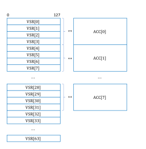
Figure 1: The MMA facility adds eight 512-bit accumulator registers (${\sf ACC}[0:7]$) to the Power ISA register set, which includes 64 vector-scalar registers (${\sf VSR}[0:63]$) of 128 bits each. Each accumulator is associated with a group of four consecutive 128-bit vector-scalar registers. The ${\sf VSR}[32:63]$ vector-scalar registers are not associated with, nor do they conflict with, any accumulator.

 

II-B MMA instructions

MMA instructions fall into one of three categories:

1. Accumulator Move Instructions: These instructions move data between the accumulator registers and their associated vector-scalar registers. (See Table I(a).)

2. Integer rank-$k$ Update Instruction: These are integer arithmetic instructions that update the elements of an accumulator with the product of input matrices. (See Table I(b).)

3. Floating-point rank-$k$ Update Instructions: These are floating-point arithmetic instructions that update the elements of an accumulator with the product of input matrices and/or vectors. (See Table I(c).)

The arithmetic instructions (integer and floating-point) have both a prefix form, which always begins with pm, and a conventional form, without the prefix. We will start our discussion with the conventional forms of the instructions and cover the prefix forms later.

 

TABLE I: MMA instructions. Those instructions with a pm prefix belong to the new class of prefix instructions in Power ISA, which are 64 bits in size. The others have the traditional format (32-bit fixed size). The arithmetic instructions have an optional 2-letter suffix that indicates how the product of the input matrices should be added to the target accumulator: pp – positive product, positive accumulator, np – negative product, positive accumulator, pn – positive product, negative accumulator, nn – negative product, negative accumulator. The optional s suffix indicates the use of saturating arithmetic for the integer instructions.

(a) Accumulator Move Instructions. Instruction Description xxsetaccz Set all elements of the target accumulator to 0 xxmfacc Move the contents of the source accumulator to the associated vector-scalar registers xxmtacc Move the contents of a group of vector-scalar registers to the associated accumulator

(b) Integer rank-$k$ update instructions. Instruction Description [pm]xvi16ger2[s][pp] Update a $4\times 4$ matrix of int32 elements with the product of two $4\times 2$ matrices of int16 elements [pm]xvi8ger4[pp,spp] Update a $4\times 4$ matrix of int32 elements with the product of two $4\times 4$ matrices of int8/uint8 elements [pm]xvi4ger8[pp] Update a $4\times 4$ matrix of int32 elements with the product of two $4\times 8$ matrices of int4 elements

(c) Floating-point rank-$k$ update instructions. Instruction Description [pm]xvbf16ger2[pp,np,pn,nn] Update a $4\times 4$ matrix of fp32 elements with the product of two $4\times 2$ matrices of bfloat16 elements [pm]xvf16ger2[pp,np,pn,nn] Update a $4\times 4$ matrix of fp32 elements with the product of two $4\times 2$ matrices of fp16 elements [pm]xvf32ger[pp,np,pn,nn] Update a $4\times 4$ matrix of fp32 elements with the product of two $4$-element vectors of fp32 elements [pm]xvf64ger[pp,np,pn,nn] Update a $4\times 2$ matrix of fp64 elements with the product of $4/2$-element vectors of fp64 elements

 

II-B1 Accumulator Move Instructions

The three Accumulator Move Instructions can be used to initialize the elements of an accumulator to 0, to move data from vector-scalar registers into an accumulator register, or to move data from an accumulator register into vector-scalar registers. When data is moved from vector-scalar registers into an accumulator, or when the accumulator elements are initialized to zero, the accumulator is said to be primed. From this point on, the associated vector-scalar registers should not be used again, until the accumulator is deprimed by moving data from the accumulator into the associated vector-scalar registers. After a depriming event, an accumulator should not be used until primed again. (See below for other instructions that prime accumulators).

II-B2 Integer rank-$k$ Update Instructions

These instructions have the general form

$$A\leftarrow XY^{T}[+A]$$ (1)

where $A$ is an accumulator register, holding a $4\times 4$ matrix of int32 elements and $X$ and $Y$ are vector-scalar registers, that must not overlap the accumulator, holding matrices of either 16-, 8- or 4-bit integers. (The bracketed term $[+A]$ is optional and $Y^{T}$ denotes the transpose of $Y$.) The exact shape of the input matrices depends on the type of input data, which also defines the value of $k$ in the rank-$k$ update operation.

Vector-scalar registers in Power ISA are always 128 bits wide. Therefore, when the input data are 16-bit integers (int16), the $X$ and $Y$ registers are interpreted as $4\times 2$ matrices, so that $XY^{T}$ produces a $4\times 4$ matrix as a result. That product matrix can be optionally added to the current value of the accumulator or directly stored in the accumulator. Instructions that simply write the value of $XY^{T}$ into the target accumulator automatically prime that accumulator. The accumulation form of the instructions, with the pp suffix in case of integer types, require that the target accumulator be previously primed with an initial value.

When using 16-bit integer inputs, with the xvi16ger2 instructions, there are two choices for the arithmetic model: the more conventional modulo arithmetic, where the largest representable integer is followed by the smallest representable integer, and saturating arithmetic model, where adding positive values to the largest representable integer or negative values to the smallest representable integer does not change the target value. Instructions with the s suffix (e.g., xvi16ger2s) use the saturating model.

For 8-bit integer inputs, with the xvi8ger4 instructions, the $X$ and $Y$ registers are interpreted as $4\times 4$ matrices. Whereas the contents of $X$ are a $4\times 4$ matrix of signed 8-bit integer elements (int8), the contents of $Y$ are a $4\times 4$ matrix of unsigned 8-bit integer elements (uint8). This mixing of signed and unsigned 8-bit integer inputs has been common practice since early generations of vector instructions, and is also present in modern deep learning libraries [17]. As with the 16-bit inputs case, the product can be optionally added to the current value of the accumulator. The same requirements regarding automatic priming of the target accumulator also hold.

The xvi8ger4 instructions offer the same choice of modulo vs saturating arithmetic as the xvi16ger2 instructions. Saturating arithmetic is only available in the accumulation-form of the instruction (suffix spp), since a product of $4\times 4$ 8-bit matrices cannot overflow a 32-bit integer result.

The final family of integer rank-$k$ update instructions consist of the xvi4ger8 instructions. In this case, the $X$ and $Y$ registers are interpreted as $4\times 8$ matrices of signed 4-bit integer elements (int4). The product $XY^{T}$ can be optionally added to the contents of the target accumulator (suffix pp). It is unlikely for a sum of products of 4-bit inputs to overflow a 32-bit accumulator. Therefore, only a modulo arithmetic version of this operation is provided.

II-B3 Floating-point rank-$k$ Update Instructions

These instructions have the general form

$$A\leftarrow[-]XY^{T}[{\pm}A]$$ (2)

where $A$ is an accumulator register, holding either a $4\times 2$ matrix of double-precision (fp64) elements or a $4\times 4$ matrix of single-precision (fp32) elements. $X$ and $Y$ are vector-scalar registers, that must not overlap the accumulator, holding matrices or vectors of 16-, 32- or 64-bit floating-point values. (In one case discussed below, $X$ is a pair of vector-scalar registers.) The product of the input matrices or vectors can be optionally negated, and then added or subtracted to the current contents of the target accumulator. The optional pp, np, pn, and nn suffixes control the accumulation operation. The first p/n in the suffix specifies either a positive or negated product and the second p/n specifies either a positive or negated accumulator.

There are two families of rank-2 update instructions for 16-bit input elements. The xvbf16ger2 instructions treat the inputs in brain float 16 format (bf16) [23], whereas the xvf16ger2 instructions treat the inputs in IEEE half-precision format (fp16) [5]. In both cases, $X$ and $Y$ are $4\times 2$ matrices of 16-bit elements, producing a $4\times 4$ matrix product (optionally negated) that can then be added to the (optionally negated) target accumulator. Just as with the integer rank-$k$ update instructions, the nonaccumulation-form of the floating-point instructions automatically prime the target accumulator.

For 32-bit inputs, the xvf32ger instructions use $X$ and $Y$ as 4-element vectors of single-precision (fp32) values, computing a $4\times 4$ outer-product that can then be optionally negated and added to the (optionally negated) target accumulator.

The double-precision instructions xvf64ger break the usual conventions for the rank-$k$ update instructions. First, the accumulator is treated as a $4\times 2$ matrix of double-precision elements (fp64). The $X$ input is a $4$-element vector of fp64 values (consisting of an even-odd pair of adjacent vector-scalar registers) and the $Y$ input is a $2$-element vector of fp64 values. None of the input vector-scalar registers can overlap the accumulator. The $XY^{T}$ outer-product is computed, producing a $4\times 2$ result. That result is optionally negated and added to the (optionally negated) accumulator.

II-C Prefixed instructions

Power ISA™ Version 3.1 introduces prefixed instructions. Whereas all Power ISA instructions pre-dating Version 3.1 consist of a single 32-bit word encoding, prefixed instructions are 64 bits long, consisting of a 32-bit prefix word followed by a 32-bit suffix word.

Each of the integer and floating-point rank-$k$ update instructions in the MMA facility has a prefix version that extends the previously discussed functionality of the base instruction. That extended functionality consists of immediate mask fields that specify the exact rows of $X$ and columns of $Y^{T}$ to be used in the computation. When the MMA instruction is of rank 2 or higher ($k\geq 2$), a third product mask field can specify the exact outer products to use when computing the result.

The masking feature of the prefixed variants is better illustrated with an example. Consider the multiplication of two $4\times 2$ matrices $X$ and $Y$ of half-precision floating-point elements (fp16) through the instruction

pmxvf16ger2pp $A$, $X$, $Y$, $x$, $y$, $p$

where $A$ is the accumulator, $x$ and $y$ are the 4-bit immediate fields specifying the masks for input matrices $X$ and $Y$ respectively, and $p$ is the 2-bit immediate field specifying the product mask. Let $x=x_{0}x_{1}x_{2}x_{3}$, $y=y_{0}y_{1}y_{2}y_{3}$ and $p=p_{0}p_{1}$, where the $x_{i}$, $y_{j}$ and $p_{k}$ are single bit values (0 or 1). The resulting value of each element $A_{ij}$ of accumulator $A$ is computed by

$$A_{ij}\leftarrow\sum_{k=0,1}[(p_{k}(x_{i}X_{ik}\times y_{j}Y_{jk})]+A_{ij}.$$ (3)

In other words, the $x$ mask enables/disables rows of $X$, the $y$ mask enables/disables columns of $Y^{T}$ and the $p$ mask enables/disables the specific partial products along the inner dimension (the $k$ from rank-$k$) of the matrix multiply. Computations on disabled rows and columns are not performed and, therefore, exceptions are not generated for those computations.

The prefix variant of the rank-$k$ update instructions can be used to compute operations on matrices of shape different than the shape directly supported by the conventional instructions. This can be useful when computing residual loop iterations after a matrix is blocked into multiples of the default size. For the xvf32ger and xvf64ger families of instructions, only the $x$ and $y$ masks can be specified, since the rank of those operations is always one ($k=1$).

III Implementation in the POWER10 processor

Figure 2 is a block diagram for the backend of the POWER10 core. Only a subset of the backend, relevant to the execution of MMA instructions, is illustrated. We do not cover aspects of the execution of either scalar instructions or load/store instructions, which are not relevant to the execution of matrix instructions.

The backend consists of four (4) execution slices (ES$[0:3]$) and an attached matrix math engine (MME). An execution slice contains a register file (VS RF) for the 128-bit wide vector-scalar registers and an execution unit (VU) for performing operations on those registers. On a given cycle, each slice can issue one instruction for execution. Slices 2 and 3 can issue either a vector instruction or an MMA instruction. Slices 0 and 1 can only issue vector instructions.

 

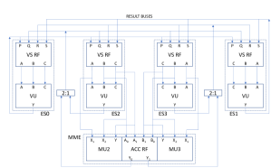
Figure 2: Block diagram of how the matrix math unit interacts with the rest of the POWER10 core. All buses shown are 128 bits wide.

 

The matrix math engine logically consists of two (2) execution pipelines (MU2 and MU3 for instructions issued from slices 2 and 3, respectively) sharing a common accumulator register file (ACC RF). This organization supports the execution of two rank-$k$ update instructions per cycle.

The physical implementation of the MME is shown in Figure 3 and consists of a $4\times 2$ grid of processing units (PU). Each processing unit has two identical halves, one for each of the issuing slices (2 and 3). Each half includes a 64-bit slice of the accumulator register file (ACC2 and ACC3) with two read and one write ports. The arithmetic and logic unit in each half (ALU2 and ALU3) can perform one double-precision or two single-precision floating-point multiply-add(s). It can also perform 4, 8, or 16 multiply-adds of 16-, 8-, or 4-bit data, respectively. The result of each ALU is always written to the corresponding accumulator register file but the input can come from either one. (Hence the requirement for two read ports.)

Whereas the accumulators (both input and output) of each instruction are stored in the accumulator register file, the $X$ and $Y$ inputs are sourced from two of the vector-scalar register files. The fetch buses from the vector-scalar register files bring $X$ and $Y$ operands for the outer product instructions and transfer data from the vector-scalar registers to the accumulators. The result buses transfer data from accumulators to the vector-scalar registers. It takes two (2) cycles to transfer four (4) vector-scalar registers to an accumulator and four (4) cycles to transfer one accumulator to 4 vector-scalar registers. Up to two transfers can be performed simultaneously.

During the computation phase of a math kernel, the accumulator data stays local to the matrix math engine. Only the $X$ and $Y$ inputs have to be brought from the register files. Furthermore, no output is placed on the results buses. This leads to a more power efficient execution of those kernels.

We compare the current MMA approach using the POWER10 matrix math engine (MME) with two other alternatives to improving the performance of processors for dense numerical linear algebra kernels: (1) expanding the vector width and (2) building a dedicated matrix-multiply unit.

The more conventional approach of widening the vector registers and vector units has been adopted by several products [6, 14, 1]. When comparing it to the approach adopted in the matrix math facility:

1. The new matrix math facility instructions have no impact to the rest of the architecture (vector registers and vector instructions stay exactly the same) and minimal impact to the micro-architecture (the matrix math engine is attached to the execution slices, which do not require any change in supporting their operations.) In contrast, widening vectors would require deeper architectural changes, either in the form of new instructions [18] or switching to a scalable vector approach [22], wider vector registers, and wider vector units.

2. When performing a $4\times 4$ outer-product of single-precision (32-bit) floating-point data, only $2\times 128$-bit vector registers have to be transmitted from the register file to the matrix math engine. The much larger $512$-bit accumulator resides entirely within the matrix math engine. A comparable $512$-bit wide vector unit would require $3\times 512$-bit registers to be fetched and one to be written back to the register file for the same 16 (single-precision) floating-point multiply-add operations.

3. The physical design of the matrix math engine has a natural two-dimensional layout (see Figure 3) that follows the structure of the outer-product computation (either $4\times 2$ for double-precision or $4\times 4$ for narrower data types). Vector computations are naturally one-dimensional and may need additional constructs to fold into two-dimensional arrangements.

4. The outer product is a BLAS2 operation and the natural algorithmic operation for the most important dense numerical linear algebra kernels. It is directly supported by the instructions of the matrix math facility. In comparison, processors with vector instructions require additional steps to transform a two-dimensional BLAS2 outer product into one-dimensional BLAS1 operations that are supported by the vector instructions. Those additional operations can include broadcast loads or splat instructions.

5. The issue-to-issue latency for the matrix math facility instructions is reduced when compared to comparable vector instructions, since the accumulators are already in the functional unit, as opposed to vector registers that are fetched from a separate register file.

 

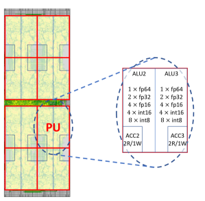
Figure 3: Each matrix unit consists of a $4\times 2$ grid of basic tiles. Each tile has a 64-bit slice of the accumulator register file (each accumulator is 512 bits wide) and the corresponding multiply-add functional units to operate on that data slice.

 

Another emerging approach is to build a dedicated matrix multiply unit, either to the core or at the chip level. This solution compares to the matrix math facility as follows:

1. The instructions of the matrix math facility are part of the instruction stream of a thread and much finer grain than a complete matrix multiplication.

2. The instructions of the matrix math facility can be used as building blocks of other computations, such as convolution, triangular solve and discrete Fourier transform.

IV Programming the MMA facility

Generation of MMA facility code from high-level language constructs is an active area of research. Currently, most code that uses those new instructions is manually generated, with explicit invocation of the new operations. While directly programming in assembly instructions is always an option for MMA exploitation, we advocate the use of compiler built-ins as a preferred alternative [7].

Built-ins are functions with pre-defined semantics, known to the compiler. The compiler can directly emit code for these built-in functions, and quite often they translate one-to-one to native machine instructions. They represent a compromise in abstraction. The programmer has detailed control of the operations performed by the machine while implementation of the built-ins in the compiler can choose to include additional semantics about the instructions. This additional information can then be used throughout the compilation process to enable optimizations. Furthermore, low-level optimizations such as instruction scheduling and register allocation are left to the compiler.

The open source GNU Compiler Collection (GCC), starting with version 10.2, has already been augmented with built-ins for the MMA facility, while work on Clang/LLVM compilers is under way. This is in addition to the various built-ins that were already implemented, including architecture agnostic and Power ISA-specific built-ins. This provides performance and functional portability across the different compilers. For this reason, and the simplicity compared with direct assembly programming, we believe programming with built-ins is the preferred approach for broader exploitation of the MMA facility.

MMA built-ins make use of three data types to specify data manipulated by those built-ins:

__vector unsigned char – a 16-byte vector, used for most rank-$1$ update operations
__vector_pair – a 32-byte vector, used for the fp64 rank-$k$ update operations
__vector_quad – a 64-byte accumulator

The new MMA built-ins are summarized in Table II. Most built-ins correspond one-to-one to machine instructions, as shown in the table. Two of the built-ins provide an ancillary role to the compiler, by constructing accumulators from vectors and extracting vectors from accumulators.

 

TABLE II: MMA built-ins. Each MMA instruction has a corresponding built-in function with pre-defined semantics known to the compiler. By programming with built-ins, the programmer can specify the exact operations to be performed by the hardware, while leaving register allocation and instruction scheduling to the compiler. In the table below, $A$ represents an accumulator (and $\&A$ its address), where $x$, $y$, $z$ and $t$ are vectors. $Q$ are vector pairs, used to hold a 4-element vector of fp64 values. Finally, u2, u4 and u8 are 2-, 4- and 8-bit unsigned integer literals used to define the masks in the prefixed instructions.

Instruction	built-in
	__builtin_mma_assemble_acc($\&A$,$x$,$y$,$z$,$t$)
	__builtin_mma_disassemble_acc($\&x$,$\&A$)
xxsetaccz	__builtin_mma_xxsetaccz($\&A$)
xxmfacc	__builtin_mma_xxmfacc($\&A$)
xxmtacc	__builtin_mma_xxmtacc($\&A$)
xvi16ger2[s][pp]	__builtin_mma_xvi16ger2[s][pp]($\&A$,$x$,$y$)
pmxvi16ger2[s][pp]	__builtin_mma_pmxvi16ger2[s][pp]($\&A$,$x$,$y$,u4,u4,u2)
xvi8ger4[pp,spp]	__builtin_mma_xvi8ger4[pp,spp]($\&A$,$x$,$y$)
pmxvi8ger4[pp,spp]	__builtin_mma_pmxvi8ger4[pp,spp]($\&A$,$x$,$y$,u4,u4,u4)
xvi4ger8[pp]	__builtin_mma_xvi4ger8[ppp]($\&A$,$x$,$y$)
pmxvi4ger8[pp]	__builtin_mma_pmxvi4ger8[pp]($\&A$,$x$,$y$,u4,u4,u8)
xvbf16ger2[pp,np,pn,nn]	__builtin_mma_xvbf16ger2[pp,np,pn,nn]($\&A$,$x$,$y$)
pmxvbf16ger2[pp,np,pn,nn]	__builtin_mma_pmxvbf16ger2[pp,np,pn,nn]($\&A$,$x$,$y$,u4,u4,u2)
xvf16ger2[pp,np,pn,nn]	__builtin_mma_xvf16ger2[pp,np,pn,nn]($\&A$,$x$,$y$)
pmxvf16ger2[pp,np,pn,nn]	__builtin_mma_pmxvf16ger2[pp,np,pn,nn]($\&A$,$x$,$y$,u4,u4,u2)
xvf32ger[pp,np,pn,nn]	__builtin_mma_xvf32ger[pp,np,pn,nn]($\&A$,$x$,$y$)
pmxvf32ger[pp,np,pn,nn]	__builtin_mma_pmxvf32ger[pp,np,pn,nn]($\&A$,$x$,$y$,u4,u4)
xvf64ger[pp,np,pn,nn]	__builtin_mma_xvf64ger[pp,np,pn,nn]($\&A$,$Q$,$y$)
pmxvf64ger[pp,np,pn,nn]	__builtin_mma_pmxvf64ger[pp,np,pn,nn]($\&A$,$Q$,$y$,u4,u2)

 

The __builtin_mma_assemble_acc performs a gather operation, collecting four 16-byte vectors $x$, $y$, $z$, and $t$ into an accumulator $A$. At first glance, this built-in may seem identical to the xxmtacc instruction but that instruction (and the corresponding __builtin_mma_xxmtacc built-in) only transfers data between an accumulator and its corresponding vector-scalar registers, whereas the __builtin_mma_assemble_acc built-in can initialize an accumulator from any set of four vectors.

Similarly, the __builtin_mma_disassemble_acc built-in performs a scatter operation, extracting the contents of an accumulator into an array of vectors that can then be used individually in the code. This is different than the transfer accomplished by the xxmfacc instruction (and corresponding __builtin_mma_xxmfacc built-in). We give an illustration of using the __builtin_mma_disassemble_acc built-in in Figure 5.

When programming with built-ins, there are some general guidelines to follow in order to help the compiler generate good quality code. First, it is not advisable to explicitly use the __builtin_mma_xxmfacc and __builtin_mma_xxmtacc built-ins. Although they are provided for completeness, it is better to simply provide the compiler with the list of vectors to initialize an accumulator with, using the __builtin_mma_assemble_acc built-in. Correspondingly, it is better to just have the compiler decompose an accumulator into a group of vectors, using the __builtin_mma_disassemble_acc built-in.

Second, there are limitations to passing accumulators across function calls, and even when supported it is likely to cause a performance degradation. A possible exception to this guideline is when one can be certain the compiler will inline the function, and therefore remove superfluous copies. (This is a common practice in C++ template libraries.) For most cases, the programmer should limit accumulator usage to within a function and avoid having function calls while using accumulators.

Third, the programmer must be conscious of the actual number of accumulators supported by the architecture (8) and not create too many live accumulator objects in a function. Otherwise, the compiler may be forced to spill extra accumulators to and from memory, which also causes a performance degradation.

Finally, and this is more a rule than a guideline, the programmer must not use an accumulator that has not been primed. Accumulators can be primed either by the __builtin_mma_assemble_acc built-in, by the __builtin_mma_xxsetaccz built-in, or by any of the nonaccumulating arithmetic rank-$k$ operations.

V Case studies

We present two case studies to illustrate the use of the matrix math instructions on computations. The first case study is for the most natural application: matrix multiplication, in this case of double-precision floating point values (DGEMM). The second case study is in the computation of two-dimensional convolutions, often used in deep learning, with single-precision floating-point data (SCONV).

V-A DGEMM

DGEMM is the general matrix-multiply routine from BLAS, computing

$$C\leftarrow\alpha A^{[T]}B^{[T]}+\beta C$$ (4)

where $A$, $B$, $C$ are matrices and $\alpha$, $\beta$ are scalars, all of type double-precision floating-point. We consider here only the innermost kernel found in high-performance libraries [10].

The inner-most kernel of DGEMM computes a register-contained $m\times n$ block of matrix $C$ as the product of a $m\times k$ block of matrix $A$ and a $k\times n$ block of matrix $B$. Typically, $k\gg m$ and $k\gg n$, to help amortize the cost of loading and storing the $C$ block into/from registers.

For our example, we will use all eight architected accumulators to create a virtual $8\times 8$ accumulator of double-precision elements, as shown in Figure 4 (a). The accumulator numbers in the figure are for illustration purpose only. Since we are programming with built-ins, we cannot control the precise allocation of registers. And that is not important either. The compiler is free to choose the particular allocation that guarantees correctness and will not affect performance.

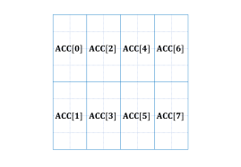
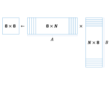
  (a) (b)  

Figure 4: The DGEMM kernel uses all architected accumulators to create a virtual $8\times 8$ accumulator of double-precision elements (a). The accumulator is used to compute the product of an $8\times N$ matrix $A$ and an $N\times 8$ matrix $B$ (b).

V-A1 The code with built-ins

Supporting definitions to make the example code more compact are shown in Figure 5. Lines 1–3 redefine the data types directly supported by the compilers to names that are more related to the computation: A 16-byte vector data type (__vector unsigned char) is used to represent a two-element vector of double-precision floating-point numbers (fp64_2), whereas a pair of vectors (__vector_pair) represents a four-element vector of double-precision floating-point numbers (fp64_4) and a group of four vectors (__vector_quad) represents a $4\times 2$ matrix of double precision floating-point numbers (fp64_4x2).

 

⬇

29typedef __vector_quad fp64_4x2;

30typedef __vector_pair fp64_4;

31typedef __vector unsigned char fp64_2;

32

33#define mma_store_acc(AS, A, D) \

34{ \

35 fp64_2 a[4]; \

36 __builtin_mma_disassemble_acc(a,&(AS)); \

37 *((fp64_2*)A+D+0) = a[0]; \

38 *((fp64_2*)A+D+1) = a[1]; \

39 *((fp64_2*)A+D+2) = a[2]; \

40 *((fp64_2*)A+D+3) = a[3]; \

41}

42

43#define mma_xvf64_8x8(acc, op, X, Y) \

44{ \

45 fp64_4 x0, x1; \

46 fp64_2 y0, y1, y2, y3; \

47 x0 = *((fp64_4*)X+0); x1 = *((fp64_4*)X+1); \

48 y0 = *((fp64_2*)Y+0); y1 = *((fp64_2*)Y+1); \

49 y2 = *((fp64_2*)Y+2); y3 = *((fp64_2*)Y+3); \

50 __builtin_mma_xvf64 ## op (&(acc[0]), x0, y0); \

51 __builtin_mma_xvf64 ## op (&(acc[1]), x0, y1); \

52 __builtin_mma_xvf64 ## op (&(acc[4]), x1, y0); \

53 __builtin_mma_xvf64 ## op (&(acc[5]), x1, y1); \

54 __builtin_mma_xvf64 ## op (&(acc[2]), x0, y2); \

55 __builtin_mma_xvf64 ## op (&(acc[3]), x0, y3); \

56 __builtin_mma_xvf64 ## op (&(acc[6]), x1, y2); \

57 __builtin_mma_xvf64 ## op (&(acc[7]), x1, y3); \

58}

Figure 5: Supporting definitions for the DGEMM kernel code.

 

Lines 5–13 define macro mma_store_acc, which stores accumulator AS in a 64-byte memory location beginning at ${\tt D}\times 16$ bytes past the address in pointer A. The accumulator is first transferred to an array of four 2-element vectors (through the built-in __builtin_mma_disassemble_acc) and then the elements are stored at consecutive 16-byte chunks of memory.

Lines 15–30 of Figure 5 define macro mma_xvf64_8x8 which computes the outer-product of two 8-element vectors of double precision floating-point numbers (X and Y), accumulating the result into an $8\times 8$ accumulator (acc) represented as an array of eight $4\times 2$ accumulators. The exact operation (accumulating or not, inverting signs or not) is specified by the op argument, which must be one of ger, gerpp, gernp, gerpn, or gernn.

The kernel function that computes the product $XY^{T}$ of two $8\times N$ double-precision matrices $X$ and $Y$ is shown in Figure 6. Line 9 tests for an empty multiply. Line 11 declares the array of $4\times 2$ accumulators that implement the virtual $8\times 8$ accumulator. Line 13 is the initial multiply without accumulation, which initializes the $8\times 8$ accumulator. Lines 15-19 are the main loop, which performs the remaining $N-1$ outer-products, with accumulation. Finally, lines 21-28 store the components of the $8\times 8$ accumulator into the result matrix A. (The layout is not conventional. That is handled in other layers of DGEMM.)

 

⬇

60void dgemm_kernel_8xNx8

61(

62 double *A,

63 const double *X,

64 const double *Y,

65 const uint64_t n

66)

67{

68 if (n == 0) return;

69

70 fp64_4x2 acc[8];

71

72 mma_xvf64_8x8(acc, ger, X, Y);

73

74 for (uint64_t i=1; i<n; i++)

75 {

76 X += 8; Y += 8;

77 mma_xvf64_8x8(acc, gerpp, X, Y);

78 }

79

80 mma_store_acc(acc[0], A, 0);

81 mma_store_acc(acc[1], A, 4);

82 mma_store_acc(acc[2], A, 8);

83 mma_store_acc(acc[3], A,12);

84 mma_store_acc(acc[4], A,16);

85 mma_store_acc(acc[5], A,20);

86 mma_store_acc(acc[6], A,24);

87 mma_store_acc(acc[7], A,28);

88}

Figure 6: DGEMM $8\times N\times 8$ kernel code.

 

V-A2 The generated machine code

We compile the source code of Figure 6 using g++ version $11.0$ in the IBM Advance Toolchain version 15.0 (alpha) [12], with the compiler flags

-mcpu=power10 -O3

which explicitly enable MMA support and higher levels of optimization.

The management of the new accumulator registers present significant challenges to their enablement in compilers. In particular, the need to transfer data to and from accumulators, and their overlap with existing vector-scalar registers, force the compiler to insert various register spill and copy operations in the intermediate representation of the code. Those are successfully removed with higher levels of optimization, which therefore are crucial to get good quality code from built-ins.

To conserve space, we limit our discussion to the object code for the loop in lines 15–19 of Figure 6, shown in Figure 7. Each column of $X$ is loaded through two 32-byte load instructions (lines 1–2) and each row of $Y^{T}$ is loaded through four 16-byte load instructions (lines 5–8). The accumulating outer-product of the two 8-element vectors is implemented by 8 xvf64gerpp instructions (lines 9–16). Lines 3 and 4 advance the pointers for $Y$ and $X$, respectively. Line 17 closes the loop.

 

⬇

1182 10001750: 40 00 a4 19 lxvp vs44,64(r4)

1183 10001754: 60 00 24 18 lxvp vs32,96(r4)

1184 10001758: 40 00 a5 38 addi r5,r5,64

1185 1000175c: 40 00 84 38 addi r4,r4,64

1186 10001760: 09 00 05 f5 lxv vs40,0(r5)

1187 10001764: 19 00 25 f5 lxv vs41,16(r5)

1188 10001768: 29 00 45 f5 lxv vs42,32(r5)

1189 1000176c: 39 00 65 f5 lxv vs43,48(r5)

1190 10001770: d6 41 0c ee xvf64gerpp a4,vs44,vs40

1191 10001774: d6 41 80 ed xvf64gerpp a3,vs32,vs40

1192 10001778: d6 49 8c ee xvf64gerpp a5,vs44,vs41

1193 1000177c: d6 49 80 ec xvf64gerpp a1,vs32,vs41

1194 10001780: d6 51 0c ef xvf64gerpp a6,vs44,vs42

1195 10001784: d6 51 00 ed xvf64gerpp a2,vs32,vs42

1196 10001788: d6 59 8c ef xvf64gerpp a7,vs44,vs43

1197 1000178c: d6 59 00 ec xvf64gerpp a0,vs32,vs43

1198 10001790: c0 ff 00 42 bdnz 10001750

Figure 7: Object code for the computation loop of the DGEMM kernel. The accumulator is updated by a sequence of $8\times 8$ outer-products of the columns of X and Y.

 

V-B SCONV

The characteristics of a convolution operation are described by a variety of parameters, including size of kernel, amount of padding, step increments, etc. In this section, we consider a simple two-dimensional convolution to illustrate this kind of computation using the new MMA instructions.

Let $h$ be a $3\times 3$ kernel, and $A$ an $m\times n$ image, both represented as matrices:

$$h = \left[\begin{array}[]{ccc}h_{0}&h_{1}&h_{2}\\ h_{3}&h_{4}&h_{5}\\ h_{6}&h_{7}&h_{8}\end{array}\right],$$ (8)

$$A = \left[\begin{array}[]{cccc}a_{0,0}&a_{0,1}&\cdots&a_{0,n-1}\\ a_{1,0}&a_{1,1}&\cdots&a_{1,n-1}\\ \vdots&\vdots&\ddots&\vdots\\ a_{m-1,0}&a_{m-1,1}&\cdots&a_{m-1,n-1}\end{array}\right].$$ (13)

We want to compute the $(m-2)\times(n-2)$ matrix $C=h*A$ which is the convolution of kernel $h$ with the image $A$ (no padding, single stepping in both dimensions). Let $C_{i},i=0,\ldots,m-3$ denote the $i$-th row of matrix $C$, which can be expressed as a vector-matrix multiplication:

$$C_{i}=\left[\begin{array}[]{ccccccccc}h_{0}&h_{1}&h_{2}&h_{3}&h_{4}&h_{5}&h_{6}&h_{7}&h_{8}\end{array}\right]\times\bar{A}_{i}$$ (15)

where $\bar{A}_{i}$ is a $9\times(m-2)$ matrix derived from $A$:

$$\bar{A}_{i} = \left[\begin{array}[]{cccc}a_{i+0,0}&a_{i+0,1}&\cdots&a_{i+0,n-3}\\ a_{i+0,1}&a_{i+0,2}&\cdots&a_{i+0,n-2}\\ a_{i+0,2}&a_{i+0,3}&\cdots&a_{i+0,n-1}\\ a_{i+1,0}&a_{i+1,1}&\cdots&a_{i+1,n-3}\\ a_{i+1,1}&a_{i+1,2}&\cdots&a_{i+1,n-2}\\ a_{i+1,2}&a_{i+1,3}&\cdots&a_{i+1,n-1}\\ a_{i+2,0}&a_{i+2,1}&\cdots&a_{i+2,n-3}\\ a_{i+2,1}&a_{i+2,2}&\cdots&a_{i+2,n-2}\\ a_{i+2,2}&a_{i+2,3}&\cdots&a_{i+2,n-1}\end{array}\right].$$ (25)

Matrix $A_{i}$ is formed by three rows of $A$, each appearing three times: once in its original form, once shifted left by one position and once shifted left by two positions.

It is common to apply multiple convolution kernels to the same input image. This can be accomplished in parallel by building a matrix $\bar{H}$ with the parameters of each kernel as a row of the matrix. If there are $k$ kernels, then $\bar{H}$ is a $k\times 9$ matrix that multiples a $9\times(m-2)$ matrix and we have transformed our convolution into a (series of) matrix multiplication(s).

Quite often, an image has multiple channels (e.g., $R$, $G$, and $B$ channels for the red, green and blue components, respectively). The multiple channels can be concatenated to form a “taller” $\bar{A}_{i}$ matrix, which is then multiplied by a ”wider” $\bar{H}$ matrix. In the 3-channel case, We end up with a $k\times 27$ by $27\times(m-2)$ matrix multiplication. This produces $k$ rows of output, one for each kernel.

When using an existing matrix-multiplication service, either a hardware engine directly or a GEMM routine in a BLAS library, one has to materialize the $\bar{A}_{i}$ matrices so that matrix multiplication can be invoked. (Some deep learning accelerators, like Google’s TPU [15], avoid this overhead by supporting convolution directly in hardware. The additional hardware required is not that significant, but it goes beyond just a matrix multiplication engine.)

With the fine-grain instructions in the MMA facility, convolution can be done directly on the input matrix $A$ by using code that is similar to the DGEMM code discussed in Section V-A. The $\bar{H}$ matrix plays the role of the left matrix and can be prepared in advance, since a kernel is typically applied repeatedly to incoming data. The image matrix $A$ plays the role of the right matrix, but each of its rows is loaded three times, each time starting at a different displacement. Once a column of $\bar{H}$ and a row of $A$ are loaded in the processors, their outer product can be computed with the same MMA instructions that would be used for a matrix multiplication.

The code for a 3-channel $3\times 3$ convolution kernel is shown in Figures 8 and 9. Figure 8 shows the supporting definitions, similar to the ones for DGEMM. The data type in this case is 32-bit single-precision floating point. The 8 architected accumulators, each holding a $4\times 4$ array of floats, are used to form an $8\times 16$ virtual accumulator. Each update operation consists of an $8\times 16$ outer product that is added to the accumulator.

 

⬇

11typedef __vector_quad fp32_4x4;

12typedef __vector unsigned char fp32_4;

13

14#define mma_store_acc(AS, A, D) \

15{ \

16 fp32_4 a[4]; \

17 __builtin_mma_disassemble_acc(a,&(AS)); \

18 *((fp32_4*)A+D+0) = a[0]; \

19 *((fp32_4*)A+D+1) = a[1]; \

20 *((fp32_4*)A+D+2) = a[2]; \

21 *((fp32_4*)A+D+3) = a[3]; \

22}

23

24#define mma_xvf32_8x16(acc, op, X, Y) \

25{ \

26 fp32_4 x0, x1; \

27 fp32_4 y0, y1, y2, y3; \

28 x0 = *((fp32_4*)X+0); x1 = *((fp32_4*)X+1); \

29 y0 = *((fp32_4*)Y+0); y1 = *((fp32_4*)Y+1); \

30 y2 = *((fp32_4*)Y+2); y3 = *((fp32_4*)Y+3); \

31 __builtin_mma_xvf32 ## op (&(acc[0]), x0, y0); \

32 __builtin_mma_xvf32 ## op (&(acc[1]), x0, y1); \

33 __builtin_mma_xvf32 ## op (&(acc[4]), x1, y0); \

34 __builtin_mma_xvf32 ## op (&(acc[5]), x1, y1); \

35 __builtin_mma_xvf32 ## op (&(acc[2]), x0, y2); \

36 __builtin_mma_xvf32 ## op (&(acc[3]), x0, y3); \

37 __builtin_mma_xvf32 ## op (&(acc[6]), x1, y2); \

38 __builtin_mma_xvf32 ## op (&(acc[7]), x1, y3); \

Figure 8: Supporting definitions for the SCONV kernel code.

 

The convolution kernel itself is shown in Figure 9. The $R$, $G$ and $B$ matrices are the the input channels, and $H$ is the matrix of kernels. $C$ is the output matrix and $n$ the number of elements per row of the input matrices. There are a total of 27 outer product operations. Three rows from each channel are used three times each, as shown in Equation 25.

 

⬇

41void sconv_kernel_8x27x16

42(

43 float *C,

44 const float *H,

45 const float *R,

46 const float *G,

47 const float *B,

48 const uint64_t n

49)

50{

51 fp32_4x4 acc[8];

52

53 mma_xvf32_8x16(acc, ger , H+ 0, R+0);

54 mma_xvf32_8x16(acc, gerpp, H+ 8, R+1);

55 mma_xvf32_8x16(acc, gerpp, H+ 16, R+2);

56

57 R += n;

58 mma_xvf32_8x16(acc, gerpp, H+ 24, R+0);

59 mma_xvf32_8x16(acc, gerpp, H+ 32, R+1);

60 mma_xvf32_8x16(acc, gerpp, H+ 40, R+2);

61

62 R += n;

63 mma_xvf32_8x16(acc, gerpp, H+ 48, R+0);

64 mma_xvf32_8x16(acc, gerpp, H+ 56, R+1);

65 mma_xvf32_8x16(acc, gerpp, H+ 64, R+2);

66

67 mma_xvf32_8x16(acc, gerpp, H+ 72, G+0);

68 mma_xvf32_8x16(acc, gerpp, H+ 80, G+1);

69 mma_xvf32_8x16(acc, gerpp, H+ 88, G+2);

70

71 G += n;

72 mma_xvf32_8x16(acc, gerpp, H+ 96, G+0);

73 mma_xvf32_8x16(acc, gerpp, H+104, G+1);

74 mma_xvf32_8x16(acc, gerpp, H+112, G+2);

75

76 G += n;

77 mma_xvf32_8x16(acc, gerpp, H+120, G+0);

78 mma_xvf32_8x16(acc, gerpp, H+128, G+1);

79 mma_xvf32_8x16(acc, gerpp, H+136, G+2);

80

81 mma_xvf32_8x16(acc, gerpp, H+144, B+0);

82 mma_xvf32_8x16(acc, gerpp, H+152, B+1);

83 mma_xvf32_8x16(acc, gerpp, H+160, B+2);

84

85 B += n;

86 mma_xvf32_8x16(acc, gerpp, H+168, B+0);

87 mma_xvf32_8x16(acc, gerpp, H+176, B+1);

88 mma_xvf32_8x16(acc, gerpp, H+184, B+2);

89

90 B += n;

91 mma_xvf32_8x16(acc, gerpp, H+192, B+0);

92 mma_xvf32_8x16(acc, gerpp, H+200, B+1);

93 mma_xvf32_8x16(acc, gerpp, H+208, B+2);

94

95 mma_store_acc(acc[0], C, 0);

96 mma_store_acc(acc[1], C, 4);

97 mma_store_acc(acc[2], C, 8);

98 mma_store_acc(acc[3], C,12);

99 mma_store_acc(acc[4], C,16);

100 mma_store_acc(acc[5], C,20);

101 mma_store_acc(acc[6], C,24);

102 mma_store_acc(acc[7], C,28);

103}

Figure 9: SCONV $8\times 27\times 16$ kernel code.

 

VI Performance measurements

We evaluate the performance of a POWER10 core with the matrix math engine using the University of Tennessee High Performance Linpack (HPL) benchmark [2]. HPL is a computation intensive benchmark with most (over 90% for large enough problems) of execution time spent on a double-precision matrix multiply kernel (DGEMM) and much of the rest in other BLAS kernels. We use the standard OpenBLAS in our distribution of Linux but we hand write the DGEMM kernel for the critical size $M=128$, $N=128$, $K=128$. The code is based on the example of Figure 6, with aggressive unrolling and other optimizations to reduce overhead.

Our experiments are performed on a preliminary hardware POWER10 platform, running at reduced clock frequency. (Both the nest and the core run at this reduced frequency.) We also use a commercially available POWER9 system and perform three types of measurements of single-core, single-thread performance: (1) We run a POWER9-compliant code that only uses POWER9 ISA instructions (vector instructions) on the commercially available POWER9 system. (2) We run exactly the same code on our preliminary POWER10 platform (labeled POWER10-VSX. (3) We run the MMA-enabled code on our preliminary POWER10 platform (labeled POWER10-MMA).

Results for the three cases are shown in Figure 10 as a function of problem size. Performance is reported in flops/cycle. As expected, overall performance increases with problem size, as a higher percentage of the computation is contained within the key $128\times 128$ DGEMM. For the larger problem sizes, vector code in POWER10 outperforms the same vector code in POWER9 by a factor of two. The POWER10 advantage is explained by it having four vector pipelines as opposed to only two in POWER9. The MMA code in POWER10 outperforms the vector code in the same platform also by a factor of two ($4\times$ better than POWER9). This is inline with the throughput of the two matrix pipelines being double that of the four vector pipes. For more performance results on both HPL and ResNet-50 (also $4\times$ the per core performance of POWER9), we refer the reader to [21].

   

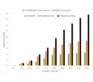
Figure 10: HPL (Linpack) performance on POWER9 and POWER10 processors.

We take a closer look at the performance of the $128\times 128$ DGEMM kernel in Figure 11. We measure the performance of an $N\times 128$ by $128\times N$ matrix multiplication for various values of N. The result is an $N\times N$ matrix and the computation makes extensive use of our $128\times 128$ DGEMM kernel.

The vector code running on the POWER9 platform achieves approximately 4.5 flops/cycle, which is 56% of the peak of 8 flops/cycle in that system. The same vector code achieves almost 10 flops/cycle (or 62% of the vector peak) on the POWER10 platform. Finally, the matrix math engine code achieves close to 26 flops/cycle (over 80% of peak) on POWER10. The improved efficiency comes from the more natural fit of the instructions to the computation, as discussed in Section III. Combined with the increased throughput of the matrix math engine, we achieve more than 2.5 times the performance of the vector code on POWER10 and more than 5.5 times the performance of the vector code on POWER9. These are better than the $4\times$ gains in HPL, since the rest of that benchmark code does not leverage the matrix math engine.

   

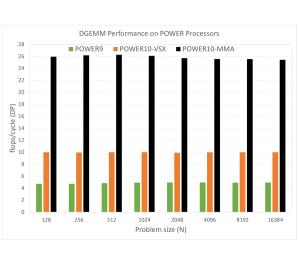
Figure 11: DGEMM performance on POWER9 and POWER10 processors, multiplying $N\times 128$ matrix $A$ and $128\times N$ matrix $B$.

VII Power efficiency aspects

We evaluate the power efficiency of our approach using a simulation-based IBM internal power methodology [8]. We run the same code used for performance evaluation (Section VI), in single-thread mode, through a detailed pre-silicon model of the core. We capture multiple 5000-instruction windows and evaluate the power draw during each window. We then average across all the windows. We measure power draw for the core without the matrix math engine, as well as just the matrix math engine itself.

The average power draw of a POWER9 and POWER10 core during execution of a $128\times 128$ DGEMM computation are shown in Figure 12. For each configuration (POWER9, POWER10 with VSX code, POWER10 with MMA code, all running at the same frequency) we show the average power of a processor core without the matrix math engine (CORE w/o MME), just the matrix math engine (MME) and total (TOTAL – the sum of the two). The POWER9 core does not have an MME, so the total is the same as just the core.

   

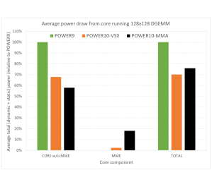
Figure 12: Average power draw of $128\times 128$ DGEMM on POWER9 and POWER10 processors.

Comparing Figures 11 and 12 we observe that the POWER10 core running MMA code delivers $2.5\times$ the performance of the same core running VSX code, while drawing only 8% more power. When the MME unit is power gated, thus eliminating any MME draw when running the VSX code, that difference increases to 12%. In any case, it is a small power increase for a significant boost in performance. If we compare to the previous generation POWER9 core, which uses an older silicon technology, we achieve a $5\times$ improvement in performance at 24% less power. This corresponds to almost $7\times$ reduction on energy per computation, looking at the core level.

VIII Conclusions

The MMA facility is a new addition to the Power ISA™ Version 3.1 that will appear in future IBM POWER processors. The facility adds a set of instructions tailored for matrix math, directly implementing rank-$k$ update of small matrices of 32-bit signed integers (with mixed-precision inputs), single-precision floating-point and double-precision floating-point numbers. The new MMA instructions are a significant departure from current vector instruction sets, which typically operate on homogeneous vector registers. The MMA instructions use vector registers as inputs, but update a new set of registers called accumulators.

It will take time for compilers to catch up with automatic code generation for the MMA facility. Meanwhile, we have augmented the GNU Compiler Collection, and are in process of augmenting LLVM-based compilers, with a new set of built-ins that match the functionality of the MMA facility. These built-ins give the programmers great control of the generated code while freeing them from details of register allocation and instruction scheduling. The source code using built-ins is easier to write and maintain than assembly code, and the generated object code is efficient, with few or no additional overhead instructions.

The matrix math engine in the IBM POWER10 processor core is the first to implement the new MMA facility instructions. It has fully achieved its objective of quadrupling the computation rate of matrix multiplication kernels over its POWER9 predecessor. That improvement has translated well to code that makes heavy use of those kernels, such as HPL.

The fine-grain nature of the MMA facility instructions mean that they can be used for various computations. We have shown in this paper how they fit into matrix multiplication and convolution. Other research work is exploring their use in stencil computations and discrete Fourier transform.

Code leveraging the MMA instructions is already included in OpenBLAS and Eigen, and can be built using the most recent versions of GCC. The uploaded OpenBLAS code supports double, single and half (bf16) precision floating-point. The new MMA instructions are present in the matrix-multiply (GEMM) kernels, which are used as building blocks for various BLAS routines.

Much of our future work consists of extending the applicability of the new MMA instructions. In addition to compiler support for automatic MMA code generation, we are also investigating what architectural features can make the MMA useful for a broader set of applications.

References

- [1] “FUJITSU Processor A64FX.” [Online]. Available: https://www.fujitsu.com/global/products/computing/servers/supercomputer/a64fx/
- [2] “HPL Benchmark.” [Online]. Available: http://icl.utk.edu/hpl/
- [3] “oneapi deep neural network library (onednn).” [Online]. Available: https://oneapi-src.github.io/oneDNN/index.html
- [4] IBM Engineering and Scientic Subroutine Library for Linux on POWER, Version 6.1, ESSL Guide and Reference. International Business Machines Corporation, 2018. [Online]. Available: https://www.ibm.com/support/knowledgecenter/SSFHY8˙6.1/reference/essl˙reference˙pdf.pdf
- [5] “IEEE Standard for Floating-Point Arithmetic,” IEEE Std 754-2019 (Revision of IEEE 754-2008), pp. 1–84, 2019.
- [6] M. Arafa, B. Fahim, S. Kottapalli, A. Kumar, L. P. Looi, S. Mandava, A. Rudoff, I. M. Steiner, B. Valentine, G. Vedaraman, and S. Vora, “Cascade lake: Next generation intel xeon scalable processor,” IEEE Micro, vol. 39, no. 2, pp. 29–36, 2019.
- [7] P. Bhat, J. Moreira, and S. K. Sadasivam, Matrix-Multiply Assist (MMA) Best Practices Guide, IBM Corporation, Ed., 2021. [Online]. Available: http://www.redbooks.ibm.com/abstracts/redp5612.html?Open
- [8] N. R. Dhanwada, D. J. Hathaway, V. V. Zyuban, P. Peng, K. Moody, W. W. Dungan, A. Joseph, R. M. Rao, and C. J. Gonzalez, “Efficient PVT independent abstraction of large IP blocks for hierarchical power analysis,” in The IEEE/ACM International Conference on Computer-Aided Design, ICCAD’13, San Jose, CA, USA, November 18-21, 2013, J. Henkel, Ed. IEEE, 2013, pp. 458–465. [Online]. Available: https://doi.org/10.1109/ICCAD.2013.6691157
- [9] J. S. Feldhousen, Intel Math Kernel Library Developer Reference. Intel Corporation, 2015. [Online]. Available: https://software.intel.com/content/www/us/en/develop/articles/mkl-reference-manual.html
- [10] K. Goto and R. A. v. d. Geijn, “Anatomy of high-performance matrix multiplication,” ACM Trans. Math. Softw., vol. 34, no. 3, May 2008.
- [11] G. Guennebaud, B. Jacob et al., “Eigen v3,” http://eigen.tuxfamily.org, 2010.
- [12] IBM Corporation, “Advance Toolchain for Linux on Power.” [Online]. Available: https://github.com/advancetoolchain/advance-toolchain
- [13] Power ISA Version 3.1, IBM Corporation, May 2020.
- [14] A. Jackson, M. Weiland, N. Brown, A. Turner, and M. Parsons, “Investigating applications on the A64FX,” in 2020 IEEE International Conference on Cluster Computing (CLUSTER). Los Alamitos, CA, USA: IEEE Computer Society, sep 2020, pp. 549–558. [Online]. Available: https://doi.ieeecomputersociety.org/10.1109/CLUSTER49012.2020.00078
- [15] N. P. Jouppi, C. Young, N. Patil, D. Patterson, G. Agrawal, R. Bajwa, S. Bates, S. Bhatia, N. Boden, A. Borchers, R. Boyle, P.-l. Cantin, C. Chao, C. Clark, J. Coriell, M. Daley, M. Dau, J. Dean, B. Gelb, T. V. Ghaemmaghami, R. Gottipati, W. Gulland, R. Hagmann, C. R. Ho, D. Hogberg, J. Hu, R. Hundt, D. Hurt, J. Ibarz, A. Jaffey, A. Jaworski, A. Kaplan, H. Khaitan, D. Killebrew, A. Koch, N. Kumar, S. Lacy, J. Laudon, J. Law, D. Le, C. Leary, Z. Liu, K. Lucke, A. Lundin, G. MacKean, A. Maggiore, M. Mahony, K. Miller, R. Nagarajan, R. Narayanaswami, R. Ni, K. Nix, T. Norrie, M. Omernick, N. Penukonda, A. Phelps, J. Ross, M. Ross, A. Salek, E. Samadiani, C. Severn, G. Sizikov, M. Snelham, J. Souter, D. Steinberg, A. Swing, M. Tan, G. Thorson, B. Tian, H. Toma, E. Tuttle, V. Vasudevan, R. Walter, W. Wang, E. Wilcox, and D. H. Yoon, “In-datacenter performance analysis of a tensor processing unit,” in Proceedings of the 44th Annual International Symposium on Computer Architecture, ser. ISCA ’17. New York, NY, USA: Association for Computing Machinery, 2017, pp. 1–12. [Online]. Available: https://doi.org/10.1145/3079856.3080246
- [16] H. Q. Le, J. V. Norstrand, B. W. Thompto, J. E. Moreira, D. Q. Nguyen, D. Hrusecky, M. Genden, and M. Kroener, “IBM POWER9 processor core,” IBM J. Res. Dev., vol. 62, no. 4/5, p. 2, 2018. [Online]. Available: http://ieeexplore.ieee.org/document/8409955/
- [17] A. F. R. Perez, B. Ziv, E. M. Fomenko, E. Meiri, and H. Shen, “Lower numerical precision deep learning inference and training,” 2018. [Online]. Available: https://software.intel.com/content/www/us/en/develop/articles/lower-numerical-precision-deep-learning-inference-and-training.html
- [18] J. R, “Intel AVX-512 Instructions,” 2017. [Online]. Available: https://software.intel.com/content/www/us/en/develop/articles/intel-avx-512-instructions.html
- [19] S. K. Sadasivam, B. W. Thompto, R. N. Kalla, and W. J. Starke, “IBM Power9 Processor Architecture,” IEEE Micro, vol. 37, no. 2, pp. 40–51, 2017. [Online]. Available: https://doi.org/10.1109/MM.2017.40
- [20] W. Starke and B. Thompto, “IBM’s POWER10 Processor,” in 2020 IEEE Hot Chips 32 Symposium (HCS), 2020, pp. 1–43. [Online]. Available: 10.1109/HCS49909.2020.9220618
- [21] W. J. Starke, B. Thompto, J. Stuecheli, and J. E. Moreira, “IBM’s POWER10 Processor,” IEEE Micro, pp. 1–1, 2021. [Online]. Available: 10.1109/MM.2021.3058632
- [22] N. Stephens, S. Biles, M. Boettcher, J. Eapen, M. Eyole, G. Gabrielli, M. Horsnell, G. Magklis, A. Martinez, N. Premillieu, and et al., “The ARM Scalable Vector Extension,” IEEE Micro, vol. 37, no. 2, pp. 26–39, Mar 2017. [Online]. Available: http://dx.doi.org/10.1109/MM.2017.35
- [23] G. Tagliavini, S. Mach, D. Rossi, A. Marongiu, and L. Benin, “A transprecision floating-point platform for ultra-low power computing,” in 2018 Design, Automation Test in Europe Conference Exhibition (DATE), 2018, pp. 1051–1056.
- [24] F. G. Van Zee and R. A. van de Geijn, “BLIS: A framework for rapidly instantiating BLAS functionality,” ACM Trans. Math. Softw., vol. 41, no. 3, Jun. 2015. [Online]. Available: https://doi.org/10.1145/2764454
- [25] Z. Xianyi, W. Qian, and W. Saar, “OpenBLAS: an optimized BLAS library,” URL http://www. openblas. net/.(Last access: 2016-05-12), vol. 1, 2016.