Quantum Corralling

Abstract

We propose a robust and efficient way to store and transport quantum information via one-dimensional discrete time quantum walks. We show how to attain an effective dispersionless wave packet evolution using only two types of local unitary operators (quantum coins or gates), properly engineered to act at predetermined times and at specific lattice sites during the system’s time evolution. In particular, we show that a qubit initially localized about a Gaussian distribution can be almost perfectly confined during long times or sent hundreds lattice sites away from its original location and later almost perfectly reconstructed using only Hadamard and $\sigma_{x}$ gates.

I Introduction

In quantum mechanics the “spreading” of the wave function is a ubiquitous characteristic of time-independent Hamiltonians bal98 ; gre00 . In this scenario, our knowledge of where a microscopic particle is located diminishes as time goes by. This natural delocalization of quantum entities is most of the time a hindrance to an efficient implementation of quantum communication protocols or to the proper execution of a quantum computational task. Indeed, the main problem of any type of communication is the ability to recover with a reasonable level of fidelity the information content sent from one point to another shannon1948mathematical and it is thus important to know where a quantum particle is located if we want to employ it as a carrier of information. In other words, we have to somehow reduce or suppress the unwanted spreading of the wave function of a quantum particle to use it efficiently as a carrier of information hua21 .

Here we pose and solve the above problem in the framework of one-dimensional discrete time quantum walks aharonov1993quantum ; kempe2003quantum . We show a very simple and robust scheme allowing an effective dispersionless time evolution of a wave package describing the position probability density of a qubit (our quantum walker). This scheme can also be adapted to efficiently store the information content of a quantum state at a given location. Actually, as we will see, we can dispersionlessly send the information, store it at another place, and send it again, repeating the previous steps many times, without disturbing the information carried by the qubit.

The present protocol is inspired and works similarly in spirit to the techniques employed by cowboys and cowgirls to herd or drive livestock from one place to another inside a cattle handling facility. This process, usually called “corralling”, aims to either send cattle from one place to another or corral it in a cattle pen. In order to drive the cattle from one place to another, a cowgirl closes a given gate while opening another one at the right place and time. By successively closing and opening gates at the right times and places, she can smoothly move the cattle from one location to another. The timing of the opening and closing of the gates has to be precise, otherwise the cattle will disperse or even move in the wrong direction. As we will see here, the protocol we describe and call “quantum corralling” works mutatis mutandis exactly in the same way. The opening and closing of gates in a cattle handling facility are substituted by the activation or inactivation of $\sigma_{x}$ gates at right times and places while the untamed cattle is a Gaussian wave packet being herded by the unitary evolution of quantum mechanics, which is not a very good herder due to its inherent dispersive aspect. See Figs. 1 to 3 and specially the videos available online as Supplementary Material to this work for a visual and easy understanding of the quantum corralling protocol.

II The protocol’s platform

Quantum walks are a promising framework to implement a variety of quantum tasks, such as quantum search algorithms shenvi2003quantum ; tulsi2008faster and universal quantum computation childs2009universal ; lovett2010universal . A rich dynamical behavior can be engineered in a quantum walk, ranging from diffusive to ballistic transport vieira2013dynamically ; vieira2014entangling ; orthey2019connecting ; li2013position ; orthey2017asymptotic ; ghizoni2019trojan ; cardano2015quantum ; su2019experimental , and many physical systems can be used to experimentally build a quantum walk wang2013physical ; venegas2012quantum . See also Refs. bos03 ; chr04 ; alb04 ; nik04 ; sub04 ; osb04 ; ple04 ; sem05 ; chr05 ; shi05 ; woj05 ; li05 ; chi05 ; kar05 ; har06 ; huo08 ; gua08 ; ban10 ; kur11 ; god12 ; apo12 ; lor13 ; sou14 ; hor14 ; shi15 ; lor15 ; zha16 ; che16 ; nic16 ; est17 ; est17a ; alm17 ; alm18 ; alm19 for quantum state transfer protocols using other platforms such as spin chains or continuous variable systems.

For our purposes, we can think of a quantum walker as a spin-$1/2$ particle (qubit) placed on a regular one-dimensional lattice where each site represents a discrete position. Its dynamical evolution is driven by a unitary operator formed by a quantum coin (gate) and a conditional displacement operator. The quantum coin acts on the qubit changing its spin state and the displacement operator moves the up (down) spin state to the right (left) adjacent position. The interference between the up spin state moving to the right with the down spin state moving to the left is the reason for the rich dynamics of quantum walks. Depending on the initial state and on the coin, we either get localization or transport of the wave function, with the latter being diffusive or ballistic.

II.1 Mathematical formalism

We now highlight the main features of the formalism and notation fully developed in Refs. vieira2013dynamically ; vieira2014entangling that are needed for our present purposes. For further details we direct the reader to those aforementioned references.

The internal degree of freedom of the quantum walker, for instance the spin of an electron or the polarization of a photon, and its external degree of freedom (position) are described by the Hilbert space $\mathcal{H}=\mathcal{H}_{C}\otimes\mathcal{H}_{P}$. Here $\mathcal{H}_{C}$ is the coin space, a complex two-dimensional vector space spanned by the vectors $\left\{\ket{\uparrow},\ket{\downarrow}\right\}$, and $\mathcal{H}_{P}$ is the position space, a numerable infinite dimensional vector space spanned by $\left\{\ket{j}\right\}$, with $j$ being an integer denoting the discrete position of the walker on a one-dimensional lattice. We assume that the information content of the walker is encoded in its internal degree of freedom.

An arbitrary initial state where the internal degree of freedom is not entangled with the position degree of freedom can be written as

$$\ket{\Psi(0)}=\left[\cos\alpha\ket{\uparrow}+e^{i\beta}\sin\alpha\ket{\downarrow}\right]\otimes\sum_{j}f(j)\ket{j},$$ (1)

where we sum over all integers $j$, $\alpha\in[0,\pi/2]$ and $\beta\in[0,2\pi]$. Note that for simplicity we set $\alpha$ to be half the polar angle $\theta$ in the Bloch sphere representation ($\theta\in[0,\pi]$) while $\beta$ is the usual azimuthal angle. Since we will be dealing with a Gaussian wave packet initially centered at the origin,

$$f(j)=Ae^{-[j^{2}/(4s^{2})]}/(2\pi s^{2})^{1/4}.$$ (2)

Here $s$ is the initial standard deviation and $A$ is a normalization constant to guarantee that $\sum_{j}|f(j)|^{2}=1$. If $j$ were a continuous variable we would have $A=1$. Eventually, in our numerical experiments, we will set $|j|\leq j_{max}$ and $A$ will be chosen to guarantee the normalization condition in this scenario.

Our main goal is to tune the time evolution of the system such that at a chosen position $j=x$, we will have at time $t$ the same wave packet we had at $t=0$ but now centered at $x$. We want $|\Psi(t)\rangle$ to be $|\Psi(0)\rangle$ displaced to position $x$. In other words, we want $|\Psi(t)\rangle=D_{x}|\Psi(0)\rangle$, where $D_{x}=\mathbb{1}_{C}\otimes\sum_{j}|j+x\rangle\langle j|$ and $\mathbb{1}_{C}$ is the identity operator in the coin space. In this case we will achieve an effective dispersionless time evolution that preserves the information encoded in the spin state: the $t=0$ spin state $\cos\alpha\ket{\uparrow}+e^{i\beta}\sin\alpha\ket{\downarrow}$ will be the spin state at $j=x$ and time $t$.

The walker’s state after $n$ discrete time steps is given by vieira2013dynamically ; vieira2014entangling

$$\ket{\Psi(n)}=\mathcal{T}\prod_{t=1}^{n}U(t)\ket{\Psi(0)},$$ (3)

where $\mathcal{T}$ indicates a time-ordered product and

$$U(t)=S\mathcal{C}(t),$$ (4)

where

$$S=\sum_{j}(\ket{\uparrow}\bra{\uparrow}\otimes\ket{j+1}\bra{j}+\ket{\downarrow}\bra{\downarrow}\otimes\ket{j-1}\bra{j})$$ (5)

is the conditional displacement operator, moving a spin up (down) to the right (left), and

$$\mathcal{C}(t)=\sum_{j}C(j,t)\otimes|j\rangle\langle j|,$$ (6)

where $C(j,t)$ is the coin operator that acts on the internal degree of freedom at position $j$ and at the time $t$. Note that in general $C(j,t)$ depends on both $j$ and $t$ and only if we have the same coin at all sites we get $\mathcal{C}(t)=C(t)\otimes\mathbb{1}_{P}$, where $\mathbb{1}_{P}$ is the identity operator in the position space. In this work we only use two coins, the Hadamard gate, $H=(\ket{\uparrow}\bra{\uparrow}+\ket{\uparrow}\bra{\downarrow}+\ket{\downarrow}\bra{\uparrow}-\ket{\downarrow}\bra{\downarrow})/\sqrt{2}$, and the not gate, $\sigma_{x}=\ket{\uparrow}\bra{\downarrow}+\ket{\downarrow}\bra{\uparrow}$.

II.2 Pure Hadamard dynamics

If in all sites we only have the Hadamard coin, namely, $\mathcal{C}(t)=H\otimes\mathbb{1}_{P}$, a Gaussian state centered at the origin as given by Eq. (1) and evolving according to Eq. (3) will split into two dispersive Gaussian wave packets, one moving to the left and the other moving to the right. Numerical analysis proves the latter claim for small and large values of the initial standard deviation $s$. For large enough $s$ and small times, we show in the Appendix A that we essentially have

$$\ket{\Psi(t)} = \ket{\psi_{R}}\otimes\sum_{j}f(j-t/\sqrt{2})|j\rangle$$ (7)

$$+(-1)^{t}\ket{\psi_{L}}\otimes\sum_{j}f(j+t/\sqrt{2})|j\rangle,$$

where $\ket{\psi_{L}}$ and $\ket{\psi_{R}}$ are orthogonal states that depend only on $\alpha$ and $\beta$. It is clear from Eq. (7) that the splitting of the initial Gaussian into two oppositely moving ones occurs regardless of the initial condition of the internal degree of freedom. Of course, for larger times the dispersion of the wave packets can no longer be ignored and the approximation above no longer applies.

We also realize looking at Eq. (7) that when only Hadamard coins are present, we cannot get a dispersionless wave packet evolution (the original wave package split into two wave packages). In order to “tame” and properly drive the wave packet in the direction we want and to obtain an effective dispersionless evolution, we need to add “gates” at specific places and leave them “closed” during a certain time interval. As we show next, this is achieved by exchanging Hadamard coins to $\sigma_{x}$ coins at certain lattice points (closing the gate) and then later, at an appropriate time, changing back to Hadamard coins (opening the gate). By proceeding in this way, we will be able to corral the wave packet.

II.3 Fidelity

Before we present more technically the protocol, it is important to define the figure of merit we will be using to verify whether or not the information content encoded in the internal degree of freedom was stored or transmitted flawlessly. We quantify the similarity between the evolved state at time $t$ with the initial one at $t=0$ by computing the fidelity between those two states: $F(t)=|\bra{\Psi(0)}D_{x}^{\dagger}\ket{\Psi(t)}|^{2}$, where $D_{x}|\Psi(0)\rangle$ is the initial state displaced to $x$, the center of the wave packet given by $|\Psi(t)\rangle$, and $D_{x}^{\dagger}$ is the adjoint of $D_{x}$. If $F=1$ the two states are the same up to an overall phase and if $F=0$ they are orthogonal.

III The protocol

Let us start showing how to keep a Gaussian state confined or corralled. Later, we will explain how to drive this Gaussian state from one place to another. As outlined above, corralling is achieved by changing the Hadamard gate to the $\sigma_{x}$ gate at specific lattice sites. The idea behind using the $\sigma_{x}$ gate is related to the fact that it acts as a not gate, changing up (down) spin states to down (up) spin states. As such, when we apply the conditional displacement after the action of this coin we will reverse the movement of the qubit. The $\sigma_{x}$ gate effectively “blocks” the passage of the qubit (similarly to the act of closing the gate while corralling cattle).

Being more specific, if initially the center of the Gaussian wave packet is located at $j_{c}=(l+r)/2$ and the left and right blocking gates are placed at positions $l$ and $r$, respectively, we must set

$$C(j,t) = \Bigg{\{}\begin{array}[]{c}\sigma_{x},\text{ if }j=l,\\ \hskip 17.07182ptH,\text{ if }l<j<r,\\ \sigma_{x},\text{ if }j=r.\end{array}$$ (11)

Numerical analysis shows that we can get an almost flawless corralling for considerably long times (of the order of thousands of time steps) and without affecting the Gaussianity of the wave packet if the $\sigma_{x}$ gates are placed at or further than three standard deviations from the wave packet’s center. This means that $l\leq j_{c}-3s$ and $r\geq j_{c}+3s$. Moreover, the analytical result reported in the Appendix A also shows that the greater the initial Gaussian width the more efficient is the present protocol. In other words, the greater the initial standard deviation the greater the fidelity of the corralled state at a given fixed time. This can be understood at the light of the Heisenberg uncertainty principle. A very narrow Gaussian in the position space implies a greater dispersion in momentum, which inevitably leads to a faster spreading of the wave packet. It is worth noting that numerical analysis shows that the efficiency of the present protocol decreases as the Gaussians become narrower. As we decrease the dispersion in position of the initial wave package, we will reach a threshold below which the present protocol cannot achieve a nearly perfect transmission (see Appendix B for details).

As a concrete illustration of what we just said, we show in Fig. 1 the average results of several numerical experiments using a Gaussian state with a fixed standard deviation $(s=10)$ and hundreds of different spin initial conditions. We work with $451$ different initial qubit states and following the notation given in Eq. (1) we pick a representative sample of values for $\alpha$ and $\beta$ that covers their entire range. We start at their lowest values and generate in increments of $\pi/20$ the remaining ones, all the way up until we reach their upper bounds. Then we work with all combinations of the previously generated values of $\alpha$ and $\beta$ as our initial conditions. This is how we get the $451$ cases of different initial qubit states. We center the Gaussian at $j_{c}=0$ and insert the $\sigma_{x}$ gates at $l=-101$ and $r=101$.

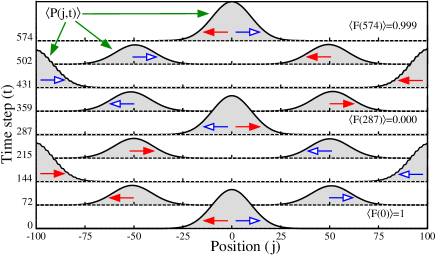
Figure 1: (color online). Average probability distribution $\langle P(j,t)\rangle$ as a function of position $j$ and time step $t$. Here $P(j,t)=|(\bra{\uparrow}\bra{j})\ket{\Psi(t)}|^{2}+|(\bra{\downarrow}\bra{j})\ket{\Psi(t)}|^{2}$. We used $451$ different spin initial conditions to compute the averages. The red and blue arrows indicate the direction of movement of the two Gaussian wave packets that split from the original one due to the dynamics of the system (Hadamard walk). The average fidelities at specific times are also shown. See text for details. Here and in all graphics all quantities are dimensionless.

In Fig. 1 the time starts at $t=0$ and after $t=287$ steps the wave package returns to its initial position, giving the same probability distribution in position space. However, due to the reflection of the two split wave packages at the $\sigma_{x}$ gates and to the dynamics associated with the Hadamard walk, the spin state when the divided wave packets first meet is orthogonal to the initial one. We need to wait another round to get the same global state, where another relative phase shift of $\pi$ between the up and down states compensates the first one. Therefore, at $t=574$ steps the system returns almost exactly to the original initial state. At this time we get an average fidelity of $0.999$.

It is worth mentioning that the previous average fidelity is computed by averaging the fidelities associated with all the $451$ different initial conditions described above. This means that the corralling works very well independently of the initial condition ascribed to the internal degree of freedom. Although not shown here, we checked the distribution for the fidelities of all the $451$ numerical experiments and we observed that all of them lie very close to the average value, corroborating the independence of the reported results on the initial spin state. Also, it is important to measure the quantum state at the right time. If we measure the state one step before or after the right time, we get zero fidelity. This is due to the $(-1)^{t}$ term appearing in Eq. (7). A measurement in an odd time leads to $(-1)^{t}=-1$, which is equivalent to a phase shift of $\pi$ and thus to the measured state being orthogonal to the initial one.

III.1 Single shot herding

Let us now move to the description of how to corral a Gaussian wave packet from one place to another, attaining at the end an effective dispersionless transmission. In this scenario there are two classes of protocols. The first one drives the Gaussian state from one corral to another in a single shot, without interrupting the driving process along the way. The second class of protocols is such that before reaching its final destination, the Gaussian wave packet is provisionally corralled in one or several intermediate corrals.

Both protocols are built on slight modifications of the previous corralling protocol, whose goal was to keep a Gaussian state confined indefinitely at a given corral. For the single shot protocol, we can drive the Gaussian state to the right if at the appropriate time we exchange the $\sigma_{x}$ coin with the Hadamard coin at the far right of the corral (we open the gate of the corral). In this way the original Gaussian wave package will move to the right in two separated wave packages, which will be corralled at another location. This is achieved by exchanging at the right time a Hadamard coin with a $\sigma_{x}$ coin at the far left of the new corral where we want to keep the Gaussian wave package confined (we are closing the gate of the corral now). See Fig. 2 for details.

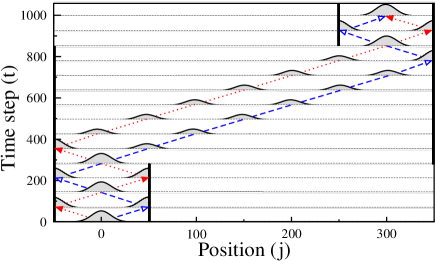
Figure 2: (color online). Average probability distribution $\braket{P(j,t)}$ as a function of the position $j$ and time $t$ using the same $451$ initial conditions employed in Fig. 1. Contrary to Fig. 1, we now employ corrals whose gates are five standard deviations away from the initial wave package’s center. The right gate ($j=50$) is opened ($\sigma_{x}$ coin changed to a Hadamard coin) when the center of both split wave packages coincide after two reflections at the gates of the corral ($t=282$). At this time we can already close the far right gate of the new corral to which we will be corralling the Gaussian state. Subsequently, half of the wave package moves to the right (dashed-blue line) and the other half, after reflecting again at the left gate of the old corral, also starts moving to the right (dotted-red line). The confinement at the new corral is achieved by closing its left gate ($j=250$) after the two wave packages’ center meet for the first time inside it ($t=849$). The average fidelity for this process at $t=995$ is $\braket{F(t)}=0.998$, which implies an almost flawless transmission.

III.2 Multiple station herding

This class of protocols is built by successive applications of the previous one, where the right gate of the previous corral is the left gate of the next one. After reaching a given corral, we repeat the single shot protocol, opening and closing the appropriate gates of the old and new corrals as explained above. Note that here we can also keep a Gaussian wave package during different times at different corrals. Furthermore, the multiple station protocol can be used to drive the qubit to a given place where a quantum gate can act upon it. In this way, going back and forth to multiple corrals, where different quantum gates are installed, we can implement a variety of quantum computational tasks. See Fig. 3 for all the details.

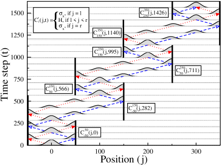
Figure 3: (color online). Same as Fig. 2 but now we have several intermediate corrals of the same size. The superscript $r$ and the subscript $l$ defining the coin operator $C^{r}_{l}(j,t)$ keep track of the location of the $\sigma_{x}$ coins. In the graphics above, the several values for the time within a given coin operator determine when it is activated and the previous one deactivated. For instance, $C_{-50}^{50}(j,0)$, $C_{-50}^{150}(j,282)$, and $C_{50}^{150}(j,566)$ imply that from $t=0$ to $t<282$ we have $\sigma_{x}$ coins (closed gates) at $j=-50$ and $j=50$ with the remaining sites given by Hadamard coins. From $t=282$ to $t<566$, the only sites where we have $\sigma_{x}$ coins are at $j=-50$ and $j=150$. At $t=566$, the $\sigma_{x}$ coins are only acting on sites $j=50$ and $j=150$. In a similar way we should read the remaining coin operators shown in the graphics. At the time $t=1566$, we have an average fidelity given by $0.997$. Again, an almost flawless transmission.

IV Disorder

In order to investigate the robustness of the quantum corralling protocol in a more realistic scenario, we will analyze its response to slight variations about the optimal settings leading to the almost perfect transmissions reported above. We will introduce errors (disorder) in the quantum coins needed to implement the quantum walk’s dynamics. And for definiteness, from now on we will work with a fixed initial spin state, namely, $(\ket{\uparrow}+i\ket{\downarrow})/\sqrt{2}$, and we will focus on the multiple station protocol, whose operation is more prone to be affected by disordered quantum coins.

An arbitrary coin can be written as vieira2013dynamically ; vieira2014entangling

$$C(j,t) = \sqrt{q(j,t)}\ket{\uparrow}\bra{\uparrow}+\sqrt{1-q(j,t)}e^{i\theta(j,t)}\ket{\uparrow}\bra{\downarrow}$$ (12)

$$+\sqrt{1-q(j,t)}e^{i\phi(j,t)}\ket{\downarrow}\bra{\uparrow}$$

$$-\sqrt{q(j,t)}e^{i[\theta(j,t)+\phi(j,t)]}\ket{\downarrow}\bra{\downarrow},$$

where $0\leq q(j,t)\leq 1$ and $-\pi\leq\theta(j,t),\phi(j,t)\leq\pi$. In this notation, the Hadamard coin is such that $q=1/2$ and $\theta=\phi=0$ while for the $\sigma_{x}$ coin we have $q=\theta=\phi=0$.

We introduce disorder in a given coin by the following prescription vieira2013dynamically ; vieira2014entangling ; vie18 ; vie19 ; vie20 ,

$$q(j,t_{n})=|q(j,t_{n-1})+\delta q(j,t_{n})|,$$

$$\theta(j,t_{n})=\theta(j,t_{n-1})+\pi\delta\theta(j,t_{n}),$$

$$\phi(j,t_{n})=\phi(j,t_{n-1})+\pi\delta\phi(j,t_{n}),$$

where $\delta q(j,t_{n}),\delta\theta(j,t_{n})$, and $\delta\phi(j,t_{n})$ are random numbers drawn from independent continuous uniform distributions defined at every $j$. All distributions are centered at zero and ranging from $-p$ to $p$. Note that for $q(j,t_{n})$ we take the absolute value of the right hand side since we must always have $q(j,t_{n})>0$. We can understand $p$ as the maximal relative variation of $q,\theta$, or $\phi$ with respect to their upper bounds. For instance, $p=0.1\%$ means that they will change from $t_{n-1}$ to $t_{n}$ by at most $\pm 0.1\%$ of their maximal allowed values. For $q$ the maximal value is $1$ while for $\theta$ and $\phi$ we have $\pi$. Also, depending on the type of disorder, $\delta q(j,t_{n}),\delta\theta(j,t_{n})$, and $\delta\phi(j,t_{n})$ are functions only of position, only of time, or of both position and time. In other words, we have, respectively, static, dynamic, or fluctuating disorder vieira2013dynamically ; vieira2014entangling ; vie18 ; vie19 ; vie20 .

Being more specific, for static disorder we randomly and independently change the optimal coin at every site $j$ according to the above prescription only once (at $t=0$). For dynamic disorder whenever $t=n\tau$, $n=1,2,3,\ldots$, and $\tau$ a predetermined period, we change every coin in the same way, i.e., using the same random number drawn from a given uniform distribution. Finally, for fluctuating disorder, whenever $t=n\tau$ we change all coins independently, similar to what we do for static disorder.

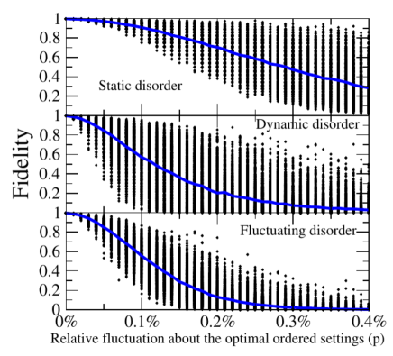
Figure 4: (color online). Top to bottom: static, dynamic, and fluctuating disorder affecting the execution of the multiple station protocol (Fig. 3). The error rate $p$ (relative fluctuation about the optimal ordered settings) varies from $0\%$ to $0.4\%$ in increments of $0.01\%$. For every value of $p$ and type of disorder we implement $1000$ disorder realizations, represented by the dots in the graphics. The average value for the fidelity is given by the solid-blue lines. The initial spin state for all cases is $(\ket{\uparrow}+i\ket{\downarrow})/\sqrt{2}$ and $\tau=10\%t_{M}$, where $t_{M}$ is the time spent by the wave packet to arrive at its last corral with optimal fidelity in the ordered protocol. See text for details.

In Fig. 4 we show how the multiple station quantum corralling protocol responds to the above three types of disorder. We realize that it is least affected by static disorder while fluctuating disorder is the most severe. Whenever the error rate is below $p=0.05\%$ we always have an average fidelity of at least $0.8$, even for fluctuating disorder. This is a quite remarkable result, in particular if we remember that we are dealing with a thousand-step protocol where errors accumulate from one step to another. Also, the present efficiency is compatible with other state of the art protocols crespi2013anderson ; gueddana2019can and we believe we can increase its efficiency at higher error rates by properly applying quantum error correction strategies at intermediate corrals aharonov1998fault ; aharonov2008fault . See also the Appendix C for a complementary analysis on the effects of disorder in the present protocol.

V Summary

Within the framework of quantum walks we proposed a very simple and robust way to store and transmit a qubit initially localized in a wave package. The present protocol, which we dubbed “quantum corralling”, uses only two types of coins, the Hadamard and the $\sigma_{x}$ coins, to effectively generate a dispersionless storage or transmission of a Gaussian wave package.

The confined or transmitted state, when measured at the right time, showed a high level of fidelity with the initial one, achieving almost unity fidelity even for walks of thousands of steps. The protocol worked independently of the initial spin state, which suggests that it can be used as building blocks to the development of dynamical quantum memories if we employ state of the art implementations of quantum walks cardano2015quantum ; su2019experimental ; crespi2013anderson ; gueddana2019can . Finally, we also envisage the use of the quantum corralling protocol to build quantum cargo protocols, where several qubits are sequentially prepared and sent using single or multiple pathways sen20 .

Appendix A Analytical proof of Eq. (7) of the main text

To analytically understand the time evolution of a Gaussian state when in all sites we have Hadamard coins (Hadamard walk), we need to work in the dual $k$-space.

Defining the two-component vector

$$\Psi(j,t)=\begin{bmatrix}\Psi_{\uparrow}(j,t)\\ \Psi_{\downarrow}(j,t)\end{bmatrix}=\begin{bmatrix}\left(\langle\uparrow|\langle j|\right)|\Psi(t)\rangle\\ \left(\langle\downarrow|\langle j|\right)|\Psi(t)\rangle\end{bmatrix},$$ (13)

where $\Psi_{\uparrow(\downarrow)}(j,t)$ is the probability amplitude of finding the qubit at position $j$ with spin up (down), the dual $k$-space is defined as follows nay00 ,

$$\tilde{\Psi}(k,t)=\sum_{j}\Psi(j,t)e^{ikj}.$$ (14)

Here the sum runs through all integers from $-\infty$ to $\infty$, $k$ is a real number such that $k\in[-\pi,\pi]$, and $\tilde{\Psi}(k,t)$ is a two component vector as well. The inverse Fourier transform is nay00

$$\Psi(j,t)=\frac{1}{2\pi}\int_{-\pi}^{\pi}\tilde{\Psi}(k,t)e^{-ikj}dk.$$ (15)

Using this notation, the initial state given in the main text [Eq. (1)] can be written as

$$\Psi(j,0)=\begin{bmatrix}\Psi_{\uparrow}(j,0)\\ \Psi_{\downarrow}(j,0)\end{bmatrix},$$ (16)

where

$$\Psi_{\uparrow}(j,0) = f(j)\cos\alpha,$$ (17)

$$\Psi_{\downarrow}(j,0) = f(j)e^{i\beta}\sin\alpha,$$ (18)

and

$$f(j)=Ae^{-[j^{2}/(4s^{2})]}/(2\pi s^{2})^{1/4}.$$ (19)

The definition and meaning of $A$ are given in the main text while $s$ is the standard deviation of the Gaussian wave packet.

Using Eqs. (14) and (16), the initial condition in the dual $k$-space is

$$\tilde{\Psi}(k,0)=\sum_{j=-\infty}^{+\infty}f(j)e^{ikj}\begin{bmatrix}\cos\alpha\\ e^{i\beta}\sin\alpha\end{bmatrix}.$$ (20)

For a large enough $s$ we can approximate the above sum for an integral. In this case $A=1$ and we get

$$\tilde{\Psi}(k,0)\approx(8\pi s^{2})^{1/4}e^{-k^{2}s^{2}}\begin{bmatrix}\cos\alpha\\ e^{i\beta}\sin\alpha\end{bmatrix}.$$ (21)

The dynamics in the $k$-space can be deduced by first obtaining the state at time $t+1$ from the one at $t$ in the position space and then using Eq. (14). Following Ref. nay00 and adapting the notation to our present problem, it is not difficult to see that $\tilde{\Psi}(k,t+1)=M_{k}\tilde{\Psi}(k,t)$, where

$$M_{k}=\frac{1}{\sqrt{2}}\begin{bmatrix}e^{ik}&e^{ik}\\ e^{-ik}&-e^{-ik}\end{bmatrix}.$$ (22)

Recursively applying this relation we get

$$\tilde{\Psi}(k,t)=(M_{k})^{t}\tilde{\Psi}(k,0).$$ (23)

If we now diagonalize $M_{k}$ we have

$$M_{k}=\lambda^{+}_{k}\ket{u_{k}^{+}}\bra{u_{k}^{+}}+\lambda^{-}_{k}\ket{u_{k}^{-}}\bra{u_{k}^{-}},$$ (24)

with eigenvalues

$$\lambda^{\pm}_{k}=\pm e^{\pm i\omega_{k}},$$ (25)

where $\omega_{k}\in[-\pi/2,\pi/2]$ and

$$\sin\omega_{k}=\frac{\sin k}{\sqrt{2}}.$$ (26)

The corresponding eigenvectors can be written as

$$\ket{u_{k}^{\pm}}=\dfrac{\begin{bmatrix}1\pm\sqrt{2}e^{i(k\pm\omega_{k})}\\ 1\end{bmatrix}}{\sqrt{2\left(1+\cos^{2}k\pm\cos k\sqrt{1+\cos^{2}k}\right)}}.$$ (27)

Therefore, inserting Eq. (24) into (23) we get

$$\tilde{\Psi}(k,t) =e^{i\omega_{k}t}\ket{u_{k}^{+}}\bra{u_{k}^{+}}\tilde{\Psi}(k,0)$$

$$+(-1)^{t}e^{-i\omega_{k}t}\ket{u_{k}^{-}}\bra{u_{k}^{-}}\tilde{\Psi}(k,0).$$ (28)

If we now use Eqs. (15), (21), (27), and (28) we obtain

$$\Psi(j,t) \approx\int_{-\pi}^{+\pi}\frac{dk}{2\pi}e^{-ikj}\left[(8\pi s^{2})^{1/4}e^{-k^{2}s^{2}}\right]\times$$

$$\left\{e^{i\omega_{k}t}g_{+}(k)\begin{bmatrix}1+\sqrt{2}e^{i(k+\omega_{k})}\\ 1\end{bmatrix}\right.$$

$$\left.+(-1)^{t}e^{-i\omega_{k}t}g_{-}(k)\begin{bmatrix}1-\sqrt{2}e^{i(k-\omega_{k})}\\ 1\end{bmatrix}\right\},$$ (29)

where

$$g_{\pm}(k)=\frac{e^{i\beta}\sin\alpha+\left(1\pm\sqrt{2}e^{-i(k\pm\omega_{k})}\right)\cos\alpha}{2\left(1+\cos^{2}k\pm\cos k\sqrt{1+\cos^{2}k}\right)}.$$ (30)

We now employ once more the assumption that $s$ is sufficiently large and also assume that $t$ is not too big. Since a large $s$ means a very narrow wave packet in the $k$-space centered about $k=0$, we can extend the above integration from $-\infty$ to $\infty$ and make the following approximations:

$$\omega_{k}t \approx \frac{k}{\sqrt{2}}t+\mathcal{O}(k^{3})t,$$ (31)

$$e^{-i(k\pm\omega_{k})} \approx 1+\mathcal{O}(k),$$ (32)

$$g_{\pm}(k) \approx \frac{e^{i\beta}\sin\alpha+(1\pm\sqrt{2})\cos\alpha}{2(2\pm\sqrt{2})}+\mathcal{O}(k).$$ (33)

Inserting Eqs. (31)-(33) into (29) and carrying out the integration we get

$$\Psi(j,t) \approx h_{+}(\alpha,\beta)\ket{R}f(j-t/\sqrt{2})$$ (34)

$$+ (-1)^{t}h_{-}(\alpha,\beta)\ket{L}f(j+t/\sqrt{2}),$$

where

$$h_{\pm}(\alpha,\beta)=\frac{e^{i\beta}\!\sin\alpha\!+\!\left(1\pm\sqrt{2}\right)\!\cos\alpha}{\sqrt{2\left(2\pm\sqrt{2}\right)}}$$ (35)

and

$$|R\rangle = \frac{1}{\sqrt{2\left(2+\sqrt{2}\right)}}\begin{bmatrix}1\!+\!\sqrt{2}\\ 1\end{bmatrix},$$ (36)

$$|L\rangle = \frac{1}{\sqrt{2\left(2-\sqrt{2}\right)}}\begin{bmatrix}1\!-\!\sqrt{2}\\ 1\end{bmatrix}.$$ (37)

Here $\ket{R}$ and $\ket{L}$ are normalized orthogonal states.

If we now define the two orthogonal states

$$|\psi_{R}\rangle = h_{+}(\alpha,\beta)|R\rangle,$$ (38)

$$|\psi_{L}\rangle = h_{-}(\alpha,\beta)|L\rangle,$$ (39)

we immediately see that we can write Eq. (34) as

$$\Psi(j,t) \approx \braket{R}{\psi_{R}}|R\rangle f(j-t/\sqrt{2})$$ (40)

$$+(-1)^{t}\braket{L}{\psi_{L}}|L\rangle f(j+t/\sqrt{2}).$$

Now, working in the $\{|R\rangle,|L\rangle\}$ basis and making the following identification,

$$\Psi(j,t)=\begin{bmatrix}\left(\langle R|\langle j|\right)|\Psi(t)\rangle\\ \left(\langle L|\langle j|\right)|\Psi(t)\rangle\end{bmatrix},$$ (41)

we have that

$$\ket{\Psi(t)} = \ket{\psi_{R}}\otimes\sum_{j}f(j-t/\sqrt{2})|j\rangle$$ (42)

$$+(-1)^{t}\ket{\psi_{L}}\otimes\sum_{j}f(j+t/\sqrt{2})|j\rangle$$

is the same as Eq. (40). And the proof is finished by noting that Eq. (42) is Eq. (7) of the main text.

Appendix B Influence of the wave package’s initial dispersion in position on the protocol’s efficiency

Here we give a more quantitative view of the efficiency of the protocol when the standard deviation in position of the initial Gaussian wave package decreases. As can be seen analyzing Fig. 5, the narrower the Gaussian wave package (lower the standard deviation), the less efficient is the protocol. The plot in Fig. 5 is made for a particular initial spin state but the general trend is similar for other initial spin states. For a standard deviation $s\geq 5.0$, we always get a fidelity of transmission at least of the order of $0.9$. As we further decrease $s$, the fidelity rapidly decreases and the present protocol is no longer the best option to transmit localized states.

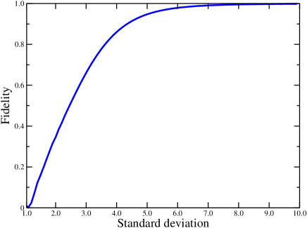
Figure 5: (color online). The data above were obtained using the same setting of Fig. 2 of the main text (single shot herding). The only difference is that we now fix our attention on one initial internal state, $(|\uparrow\rangle-i|\downarrow\rangle)/\sqrt{2}$, and change the standard deviation $s$ of the wave package from $s=10$, the value used in Fig. 2, down to $s=1.0$. For every value of $s$, we evolve the system according to the single shot herding protocol and we measure the system at the optimal time given in Fig. 2. This is the state used to compute the fidelity with the initial state for a given value of $s$.

Appendix C More on disorder

Our goal here is to investigate the response of the multiple station protocol to the following two scenarios of disorder. First, we want to know the efficiency of the protocol when the bias $q(j,t)$ of the coins are subjected to disorder while the phases are not. Second, what happens if now the phases are affected by disorder and the bias of the coins is unaffected.

Looking at Fig. 6 we realize that the system is barely affected when disorder is present only in the phases. The relevant parameter which determines the whole fate of the protocol in the presence of disorder is the bias $q(j,t)$. Comparing the upper panel with the middle one, we see that they lead to almost the same fidelities. The lower panel shows that when only the phases are subjected to disorder, we can have a much greater value of error $p$ without appreciably affecting the efficiency of the protocol.

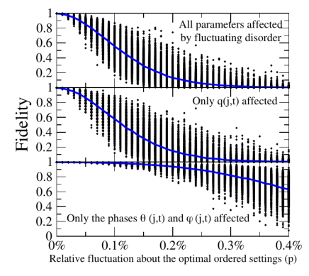
Figure 6: (color online). The upper panel is exactly the lower panel of Fig. 4 of the main text, where fluctuating disorder is introduced in the multiple station corralling protocol, affecting all parameters of the coins, namely, $q(j,t)$, $\theta(j,t)$, and $\phi(j,t)$. We also employ the same notation in the middle and lower panels. The data of the other panels were computed using the same settings and number of disorder realizations for each $p$ as given in Fig. 4 of the main text, with the following modifications. Middle panel: Fluctuating disorder acting only on the parameters $q(j,t)$ defining the Hadamard and $\sigma_{x}$ coins. The phases are not affected by disorder. Lower panel: Fluctuating disorder acting only on the phases, the bias $q(j,t)$ of the coins are not affected.

We also checked a possible decrease in the efficiency of the protocol when we measure the transmitted quantum state at a different time than the optimal one predicted by the clean model. The first thing worth noticing is the fact that if we measure the state one time step before or after the right time $t_{M}$ we get zero fidelity. This is related to the $(-1)^{t}$ relative phase between the two split wave packages, as depicted in Eq. (7) of the main text [Eq. (42) here]. Actually, if we measure the wave package at odd times we will always get a relative $\pi$ phase, i.e., $(-1)^{t_{odd}}=-1$. In this case we have to apply an appropriate phase flip gate to compensate for this phase. For even times, but not too distant from the correct measuring time, we get very high fidelities, almost as high as if we had measured at the right time. With that in mind, we tested what would happen if we deviate about $t_{M}$, detecting the state before or after the right time. We observed that for deviations of the order $\pm 10\%$ about $t_{M}$, no appreciable reduction in the fidelity occurred. We still get in this scenario an average fidelity greater than $0.9$.

Finally, we also investigated how fluctuations about the right time to change the Hadamard coin to a $\sigma_{x}$ coin (closing the gate) or vice-versa affected the protocol. The decrease in the efficiency of the protocol was negligible to deviations of the order $\pm 10\%$ about the correct time to switch one coin to the other. This comes about because the switching of the coins occurs several standard deviations away from the center of the wave package.

Appendix D Description of the accompanying videos

The file “single_shot_corralling.mp4” is the animation of the single shot protocol as given in Fig. 2 of the main text using the state $(|\uparrow\rangle+i|\downarrow\rangle)/\sqrt{2}$ as the initial spin state. For every integer $t$, from $t=0$ to $t=995$ steps, we have computed the probability distribution and then animated those $996$ frames. The green vertical bars mark the lattice sites where a Hadamard coin was changed to a $\sigma_{x}$ coin (closing the gate).

The file “multiple_station_corralling.mp4” is the animation of the multiple station protocol as given in Fig. 3 of the main text using the state $(|\uparrow\rangle+i|\downarrow\rangle)/\sqrt{2}$ as the initial qubit state. For every integer $t$, from $t=0$ to $t=1566$, we have computed the probability distribution and then animated those $1567$ frames. The green vertical bars mark where a Hadamard coin was changed to a $\sigma_{x}$ coin (closing the gate).

References

- (1) L. E. Ballentine, Quantum Mechanics: A Modern Development (World Scientific, Singapore, 1998).
- (2) W. Greiner, Relativistic Quantum Mechanics: Wave Equations (Springer-Verlag, Berlin, 2000).
- (3) C. E. Shannon, Bell System Technical Journal 27, 379 (1948).
- (4) Z. Huang, A. Clerk, and I. Martin, Phys. Rev. Lett. 126, 100601 (2021).
- (5) Y. Aharonov, L. Davidovich, and N. Zagury, Phys. Rev. A 48, 1687 (1993).
- (6) J. Kempe, Contemp. Phys. 44, 307 (2003).
- (7) N. Shenvi, J. Kempe, and K. B. Whaley, Phys. Rev. A 67, 052307 (2003).
- (8) A. Tulsi, Phys. Rev. A 78, 012310 (2008).
- (9) A. M. Childs, Phys. Rev. Lett. 102, 180501 (2009).
- (10) N. B. Lovett, S. Cooper, M. Everitt, M. Trevers, and V. Kendon, Phys. Rev. A 81, 042330 (2010).
- (11) R. Vieira, E. P. M. Amorim, and G. Rigolin, Phys. Rev. Lett. 111, 180503 (2013).
- (12) R. Vieira, E. P. M. Amorim, and G. Rigolin, Phys. Rev. A 89, 042307 (2014).
- (13) Z. J. Li, J. A. Izaac, and J. B. Wang, Phys. Rev. A 87, 012314 (2013).
- (14) A. C. Orthey and E. P. M. Amorim, Phys. Rev. A 99, 032320 (2019).
- (15) A. C. Orthey and E. P. M. Amorim, Quantum Inf. Process. 16, 224 (2017).
- (16) H. S. Ghizoni and E. P. M. Amorim, Braz. J. Phys. 49, 168 (2019).
- (17) F. Cardano, F. Massa, H. Qassim, E. Karimi, S. Slussarenko, D. Paparo, C. de Lisio, F. Sciarrino, E. Santamato, R. W. Boyd, and L. Marrucci, Sci. Adv. 1, e1500087 (2015).
- (18) Q.-P. Su, Y. Zhang, L. Yu, J.-Q. Zhou, J.-S. Jin, X.-Q. Xu, S.-J. Xiong, Q. Xu, Z. Sun, K. Chen, F. Nori, and C.-P. Yang, npj Quantum Inf. 5, 40 (2019).
- (19) K. Manouchehri and J. Wang, Physical Implementation of Quantum Walks (Springer-Verlag, Berlin, 2014).
- (20) S. E. Venegas-Andraca, Quantum Inf. Process. 11, 1015 (2012).
- (21) S. Bose, Phys. Rev. Lett. 91, 207901 (2003).
- (22) M. Christandl, N. Datta, A. Ekert, and A. J. Landahl, Phys. Rev. Lett. 92, 187902 (2004).
- (23) C. Albanese, M. Christandl, N. Datta, and A. Ekert, Phys. Rev. Lett. 93, 230502 (2004).
- (24) G. M. Nikolopoulos, D. Petrosyan, and P. L. Lambropoulos, J. Phys.: Condens. Matter 16, 4991 (2004).
- (25) V. Subrahmanyam, Phys. Rev. A 69, 034304 (2004).
- (26) T. J. Osborne and N. Linden, Phys. Rev. A 69, 052315 (2004).
- (27) M. B. Plenio, J. Hartley, and J. Eisert, New J. Phys. 6, 36 (2004).
- (28) M. B. Plenio and F. L. Semião, New J. Phys. 7, 73 (2005).
- (29) M. Christandl, N. Datta, T. C. Dorlas, A. Ekert, A. Kay, and A. J. Landahl, Phys. Rev. A 71, 032312 (2005).
- (30) T. Shi, Y. Li, Z. Song, and Ch.-P. Sun, Phys. Rev. A 71, 032309 (2005).
- (31) A. Wójcik, T. Łuczak, P. Kurzyński, A. Grudka, T. Gdala, and M. Bednarska, Phys. Rev. A 72, 034303 (2005).
- (32) Y. Li, T. Shi, B. Chen, Z. Song, and C.-P. Sun, Phys. Rev. A 71, 022301 (2005).
- (33) G. De Chiara, D. Rossini, S. Montangero, and R. Fazio, Phys. Rev. A 72, 012323 (2005).
- (34) P. Karbach and J. Stolze, Phys. Rev. A 72, 030301 (2005).
- (35) M. J. Hartmann, M. E. Reuter, and M. B. Plenio, New J. Phys. 8, 94 (2006).
- (36) M. X. Huo, Y. Li, Z. Song, and C. P. Sun, Europhys. Lett. 84, 30004 (2008).
- (37) G. Gualdi, V. Kostak, I. Marzoli, and P. Tombesi, Phys. Rev. A 78, 022325 (2008).
- (38) L. Banchi, T. J. G. Apollaro, A. Cuccoli, R. Vaia, and P. Verrucchi, Phys. Rev. A 82, 052321 (2010).
- (39) P. Kurzyński and A. Wójcik, Phys. Rev. A 83, 062315 (2011).
- (40) C. Godsil, S. Kirkland, S. Severini, and J. Smith, Phys. Rev. Lett. 109, 050502 (2012).
- (41) T. J. G. Apollaro, L. Banchi, A. Cuccoli, R. Vaia, and P. Verrucchi, Phys. Rev. A 85, 052319 (2012).
- (42) S. Lorenzo, T. J. G. Apollaro, A. Sindona, and F. Plastina, Phys. Rev. A 87, 042313 (2013).
- (43) R. Sousa and Y. Omar, New J. Phys. 16, 123003 (2014).
- (44) K. Korzekwa, P. Machnikowski, and P. Horodecki, Phys. Rev. A 89, 062301 (2014).
- (45) Z. C. Shi, X. L. Zhao, and X. X. Yi, Phys. Rev. A 91, 032301 (2015).
- (46) S. Lorenzo, T. J. G. Apollaro, S. Paganelli, G. M. Palma, and F. Plastina, Phys. Rev. A 91, 042321 (2015).
- (47) X.-P. Zhang, B. Shao, S. Hu, J. Zou, and L.-A. Wu, Ann. Phys. (NY) 375, 435 (2016).
- (48) X. Chen, R. Mereau, and D. L. Feder, Phys. Rev. A 93, 012343 (2016).
- (49) F. Nicacio and F. L. Semião, Phys. Rev. A 94, 012327 (2016).
- (50) M. P. Estarellas, I. D’Amico, and T. P. Spiller, Sci. Rep. 7, 42904 (2017).
- (51) M. P. Estarellas, I. D’Amico, and T.P. Spiller, Phys. Rev. A 95, 042335 (2017).
- (52) G. M. A. Almeida, F. A. B. F. de Moura, T. J. G. Apollaro, and M. L. Lyra, Phys. Rev. A 96, 032315 (2017).
- (53) G. M. A. Almeida, F. A. B. F. de Moura, and M. L. Lyra, Phys. Lett. A 382, 1335 (2018).
- (54) G. M. A. Almeida, F. A. B. F. de Moura, and M. L. Lyra, Quantum Inf. Process. 18, 41 (2019).
- (55) A. Crespi, R. Osellame, R. Ramponi, V. Giovannetti, R. Fazio, L. Sansoni, F. De Nicola, F. Sciarrino, and P. Mataloni, Nature Photonics 7, 322 (2013).
- (56) A. Gueddana, P. Gholami, and V. Lakshminarayanan, Quantum Inf. Process. 18, 221 (2019).
- (57) D. Aharonov and M. Ben-Or, Fault Tolerant Quantum Computation with Constant Error, in Proceedings of the twenty-ninth annual ACM symposium on Theory of computing, El Paso, Texas, USA, p. 176. See also arXiv:quant-ph/9611025.
- (58) D. Aharonov and M. Ben-Or, SIAM J. Comput. 38, 1207 (2008).
- (59) R. Vieira and G. Rigolin, Phys. Lett. A 382, 2586 (2018).
- (60) R. Vieira and G. Rigolin, Quantum Inf. Process. 18, 135 (2019).
- (61) R. Vieira and G. Rigolin, Phys. Lett. A 384, 126536 (2020).
- (62) S. Roy, T. Das, D. Das, A. Sen(De), U. Sen, Ann. Phys. (N.Y.) 422, 168281 (2020).
- (63) A. Nayak and A. Vishwanath, arXiv:quant-ph/0010117.