Enabling Novel Interconnection Agreements
with Path-Aware Networking Architectures

Abstract

Path-aware networks (PANs) are emerging as an intriguing new paradigm with the potential to significantly improve the dependability and efficiency of networks. However, the benefits of PANs can only be realized if the adoption of such architectures is economically viable. This paper shows that PANs enable novel interconnection agreements among autonomous systems, which allow to considerably improve both economic profits and path diversity compared to today’s Internet. Specifically, by supporting packet forwarding along a path selected by the packet source, PANs do not require the Gao–Rexford conditions to ensure stability. Hence, autonomous systems can establish novel agreements, creating new paths which demonstrably improve latency and bandwidth metrics in many cases. This paper also expounds two methods to set up agreements which are Pareto-optimal, fair, and thus attractive to both parties. We further present a bargaining mechanism that allows two parties to efficiently automate agreement negotiations.

I Introduction

Path-aware networks (PANs) are an innovative networking paradigm which has the potential to improve the dependability and efficiency of networks by increasing the flexibility in packet forwarding. In contrast to today’s Internet, PANs enable end-hosts to choose the path at the level of autonomous systems (ASes), which is then embedded in the header of data packets. As such, they are not limited to using a single path between a pair of ASes, but can use all available paths simultaneously. This multi-path approach has two important consequences. First, the availability of multiple paths increases the network’s resilience to link failures and its overall capacity through the possibility to avoid congested links. Second, the possibility of path selection enables end-hosts to choose paths based on their applications’ requirements—e.g., low latency for voice-over-IP calls and high bandwidth for file transfers.

Over the past two decades, significant progress has been made regarding the technical prerequisites for realizing these PAN benefits. Numerous PAN architectures have been proposed—including Platypus [44, 45], PoMo [4], NIRA [54], Pathlets [20], NEBULA [2], and SCION [57, 42]—all of which enable end-host path selection between provider-acknowledged paths (in contrast to source routing, where end-hosts are trusted to construct paths themselves). In particular, SCION is already in production use since 2017, when a large Swiss bank switched a branch to only rely on SCION for communication with their data center. Since then, 7 ISPs are now commercially offering SCION connections [50, 1]. An important aspect of today’s SCION production deployment is that it is operating independently of BGP, so it not an overlay network over BGP.

While PAN architectures have thus experienced partial deployment, surprisingly little is known today about the interconnection agreements between ASes possible in such architectures. These interconnection agreements, however, are highly relevant for both ASes and end-hosts. From the perspective of ASes, interconnection agreements determine the economic opportunities offered by PANs, which are critical to PAN adoption. From the perspective of end-hosts, interconnection agreements play an essential role for path diversity; the extent of path diversity, in turn, influences the magnitude of above mentioned resilience and efficiency improvements of PANs.

In this context, we observe that PAN architectures enable new types of interconnection agreements that are not possible in today’s Internet. Nowadays, interconnection agreements are heavily influenced by the Gao–Rexford conditions (henceforth: GRC) [16, 10], which prescribe that traffic from peers and providers must not be forwarded to other peers or providers. It is important to distinguish between two aspects of the GRC which refer to independent concerns: a stability aspect and an economic aspect. Regarding stability, the GRC provably imply route convergence of the Border Gateway Protocol (BGP) [16], and from an economic perspective, the GRC signify that an AS only forwards traffic if the cost of forwarding can be directly recuperated from customer ASes or end hosts.

Figure 1: AS topology with interconnection agreements $a$ and $a^{\prime}$ (discussed in § III-B). Peering links are shown as dashed lines, provider–customer links as “provider $\rightarrow$ customer”.

However, PAN architectures no longer require the GRC for providing stability. While paths in PAN architectures are discovered similarly as in BGP, namely by communicating path information to neighboring ASes, data packets are forwarded along a path selected by the packet source, which is embedded in the packet headers. Thus, PAN architectures trivially solve convergence issues in the sense of achieving a consistent view of the used forwarding paths, as we will explain in § II.

PAN architectures therefore present the exciting opportunity to create and use GRC-violating paths—if such paths can be made economically viable. In particular, we observe that PAN architectures may no longer require the GRC for reasons of stability, but must still respect the economic logic that makes the GRC a rational forwarding policy. For example, while the creation of GRC-violating path $ADE$ by $D$ in Fig. 1 may not lead to convergence problems, the path still is economically undesirable for $D$, because $D$ would incur a charge from its provider $A$ for forwarding traffic of $E$, which it cannot recuperate due to $E$’s status as a peer.

In this paper, we tackle this challenge by proposing new interconnection agreements based on mutuality, a concept that is already present in peering agreements today, but can be leveraged to set up more complex and flexible agreements. Concretely, mutuality means that the mentioned example path $ADE$ could be rendered economically viable for $D$ by requiring a quid pro quo from $E$, the main beneficiary of the path. For example, $E$ could offer path $DEB$ to $D$ such that both $D$ and $E$ could save transit cost for accessing ASes $B$ and $A$, respectively, but incur additional transit cost for forwarding their peer’s traffic to their respective provider. Moreover, ASes $D$ and $E$ might as well provide each other with access to their peers $C$ and $F$, thereby saving transit cost while experiencing additional load on their network. If the flows over the new path segments are properly balanced and especially if the new path segments allow ASes $D$ and $E$ to attract additional revenue-generating traffic from their customers, such unconventional agreements can be mutually beneficial. Hence, PANs offer opportunities for profit maximization which are not present in today’s Internet.

Concluding mutuality-based agreements affects revenue and cost of the AS parties in many ways, which requires a careful structuring of such agreements. We envisage that such agreements contain conditions that must be respected in order to preserve the positive value of the agreement for both parties. To this end, we further present a formal model of AS business calculations and AS interconnections that allows to derive two different types of agreement conditions, namely conditions based on flow volumes and conditions based on cash compensation. Moreover, we show how to shape mutuality-based agreements to maximize the utility (i.e., the profit) obtained by both parties, and how to negotiate them efficiently.

Finally, we investigate the effect of mutuality-based agreements on path diversity, building on a combination of several publicly available datasets [8, 9, 7, 32]. Our results underpin the benefits of mutuality-based agreements, which provide ASes access to thousands of additional paths, many of which are considerably more attractive regarding latency and bandwidth than the previously available paths. We believe that the the highly beneficial agreements investigated in this paper could represent a catalyst to overcome the still limited deployment of PAN architectures.

II The Relevance of GRC for BGP and PANs

To clarify why the GRC are needed in a BGP/IP-based Internet but not in PAN architectures, we compare their convergence requirements using the example topology of Fig. 1.

The fundamental issue with convergence in BGP is the next-hop principle: ASes can only select a next-hop AS for their traffic and thus rely on that AS to forward the traffic along the route that was originally communicated via BGP. If this assumption is violated—even temporarily—routing loops can arise. Put differently, in a BGP/IP-based Internet, all ASes need to share a common view of the used forwarding paths.

Now suppose that ASes $D$ and $E$ forwarded routes from their respective providers $A$ and $B$ to each other, which violates the GRC. Assuming both $D$ and $E$ prefer routes learned from peers, this results in a (slightly extended) instance of the classical DISAGREE example [24], which does converge with BGP but non-deterministically. The non-determinism of such topologies, which are also known as “BGP wedgies” [22], is undesirable, but it does not constitute a fundamental problem for convergence in BGP. However, adding a single additional AS $C$, which concludes similar agreements with both $D$ and $E$, this topology leads to the famous BAD GADGET, which has been shown to cause persistent route oscillations [24].

This susceptibility to oscillations is also worrisome because seemingly benign topologies and policies may easily reduce to the BAD GADGET in case one network link fails [24]. This shows that GRC-violating policies need to be implemented very carefully and with coordination among all involved parties to ensure routing stability (e.g., using BGP communities). As a consequence, “sibling” agreements in which two ASes provide each other access to their respective providers (as presented above) generally only exist between ASes controlled by a single organization.

Unlike IP, PANs forward a packet along the path encoded in its header. Thus, there is no uncertainty about the traversed forwarding path after the next-hop AS and routing loops can be prevented. For example, if a source in $D$ would encode path $DEBA$ in packets sent to a receiver in $A$, $E$ would not send these packets back to $D$. Precautions like the GRC are therefore not required for stability in a PAN and ASes have substantially more freedom in deciding which interconnection agreements to conclude and which paths to authorize.

III Modelling Interconnection Economics

In this section, we describe our model of the economic interactions between ASes in the Internet, which allows to derive quantitative conditions that must be fulfilled by interconnection agreements.

III-A AS Business Calculation

We model the Internet as a mixed graph $\mathcal{G}=(\mathcal{A},\mathcal{L}_{\leftrightarrow},\mathcal{L}_{\uparrow})$, where the nodes $\mathcal{A}$ correspond to ASes, the undirected edges $\mathcal{L}_{\leftrightarrow}$ correspond to peering links, and the directed edges $\mathcal{L}_{\uparrow}$ correspond to provider–customer links. An edge $(X,Y)\in\mathcal{L}_{\uparrow}$ corresponds to a link from provider $X$ to customer $Y$. An AS node $X\in\mathcal{A}$ is connected to a set of neighbor ASes that can be decomposed into a provider set $\pi(X)$, a peer set $\varepsilon(X)$, and a customer set $\gamma(X)$. For simplicity of notation, we denote the customer end-hosts of $X$ as a virtual stub $\Gamma_{X}\in\gamma(X)$, connected over a virtual provider–customer link $\ell^{\prime}$.

Each provider–customer link $\ell=(X,Y)\in\mathcal{L}_{\uparrow}$ has a corresponding pricing function $p_{\ell}(f_{\ell})$, yielding the amount of money $X$ receives from $Y$ given flow volume $f_{\ell}$ on link $\ell$. This flow volume $f_{\ell}$ can be interpreted as is appropriate for the pricing function, e.g., as the median, average, or 95th percentile of traffic volume over a given time period. Each pricing function $p_{\ell}(f_{\ell})$ is of the form $\alpha_{\ell}f_{\ell}^{\beta_{\ell}}$, where $\alpha_{\ell}\geq 0$ and $\beta_{\ell}\geq 0$ are pricing-policy parameters. For example, $\beta_{\ell}=0$ corresponds to flat-rate pricing with flow-independent fee $\alpha_{\ell}$, $\beta_{\ell}=1$ corresponds to to pay-per-usage pricing with traffic-unit cost $\alpha_{\ell}$, and $\beta_{\ell}>1$ results in a superlinear pricing function, e.g., as given in congestion pricing. For simplicity, we assume that all peering links $\ell^{\prime}\in\mathcal{L}_{\leftrightarrow}$ are settlement-free, as usual in the literature [28]. Paid-peering links can be represented in the model as provider–customer links. We write $p_{XY}=p_{(X,Y)}$ for brevity.

In addition to charges defined by pricing functions, an AS $X$ incurs an internal cost according to an internal-cost function $i_{X}(f_{X})$, which is non-negative and monotonously increasing in the flow $f_{X}$ through $X$. Furthermore, let the flow $f_{XY}$ be the share of $f_{X}$ that also flows directly to or from its neighbor $Y$. These sub-flows are represented in vector $\mathbf{f}_{X}$, i.e., $(\mathbf{f}_{X})_{Y}=f_{XY}$. Analogously, $f_{XYZ}$ is the flow volume on the path segment consisting of ASes $X$, $Y$, and $Z$ in that order, independent of direction.

The utility (or profit) $\mathcal{U}_{X}(\mathbf{f}_{X})=r_{X}(\mathbf{f}_{X})-c_{X}(\mathbf{f}_{X})$ of an AS $X$ is the difference between the revenue $r_{X}(\mathbf{f}_{X})$ obtained and the costs $c_{X}(\mathbf{f}_{X})$ incurred by traffic distribution $\mathbf{f}_{X}$:

$$r_{X}(\mathbf{f}_{X}) =\sum_{Y\in\gamma(X)}p_{XY}(f_{XY}),$$ (1a)

$$c_{X}(\mathbf{f}_{X}) =i_{X}(f_{X})+\sum_{Y\in\pi(X)}p_{YX}(f_{XY}).$$ (1b)

This simple model can already formalize some important insights. For example, consider ASes $A$, $D$, and $H$ in Fig. 1, connected by provider–customer links $(A,D)$ and $(D,H)$. For $D$ to make a profit, i.e., $\mathcal{U}_{X}(\mathbf{f}_{X})>0$, it must hold that $r_{D}(\mathbf{f}_{D})>c_{D}(\mathbf{f}_{D})$. This in turn implies $p_{DH}(f_{DH})+p_{D\Gamma_{D}}(f_{D\Gamma_{D}})>p_{AD}(f_{AD})+i_{D}(f_{D})$, i.e., the revenue from $H$ and $D$’s customer end-hosts must cover the cost induced by charges from $A$ as well as internal cost.

III-B Interconnection Agreements

We denote an interconnection agreement $a$ between two ASes $X$ and $Y$ in terms of the respective neighbor ASes to which $X$ and $Y$ gain new paths thanks to the agreement:

$$a=\big{[}X(\uparrow\pi^{\prime}_{X},\rightarrow\varepsilon^{\prime}_{X},\downarrow\gamma^{\prime}_{X});Y(\uparrow\pi^{\prime}_{Y},\rightarrow\varepsilon^{\prime}_{Y},\downarrow\gamma^{\prime}_{Y})\big{]}$$ (2)

Here $\pi^{\prime}_{X}\subseteq\pi(X)$, $\varepsilon^{\prime}_{X}\subseteq\varepsilon(X)$ and $\gamma^{\prime}_{X}\subseteq\gamma(X)$ are the providers, peers, and customers of AS $X$, respectively, to which $Y$ obtains access through the agreements (analogous for $\pi^{\prime}_{Y}$, $\varepsilon^{\prime}_{Y}$, $\gamma^{\prime}_{Y}$). Furthermore, we introduce the notation $a_{X}=\pi^{\prime}_{X}\cup\varepsilon^{\prime}_{X}\cup\gamma^{\prime}_{X}$, and an analogous notation for $Y$.

Next, we formalize the utility of interconnection agreements. Let the utility $u_{X}(a)$ of agreement $a$ to $X$ be the difference in $\mathcal{U}_{X}$ produced by changes in flow composition due to agreement $a$, i.e.,

$$u_{X}(a)=\mathcal{U}_{X}(\mathbf{f}_{X}^{(a)})-\mathcal{U}_{X}(\mathbf{f}_{X})=\Delta r_{X}-\Delta c_{X},$$ (3)

where $\mathbf{f}_{X}^{(a)}$ is the distribution of traffic passing through $X$ if agreement $a$ is in force, and $\Delta r_{X}$ and $\Delta c_{X}$ are agreement-induced changes in revenue and cost of $X$, respectively.

III-B1 Example of Peering Agreement

Consider the negotiation of a classic peering agreement between ASes $D$ and $E$ in Fig. 1, which so far have been connected by providers $A$ and $B$. We assume that ASes $D$ and $E$ are pure transit ASes, i.e., there are no customer end-hosts within these ASes. In a classic peering agreement, both ASes provide each other access to all of their respective customers. Using the notation introduced above, this agreement is formalized as $a_{p}=[D(\downarrow\{H\});E(\downarrow\{I\})]$. The change in revenue for $D$,

$$\Delta r_{D}=p_{DH}(f_{DH}^{(a_{p})})-p_{DH}(f_{DH}),$$ (4)

results from changes in flows to $D$’s customer $H$, driven by the new peering link $\ell^{\prime}(D,E)$. The changes in cost to $D$,

$$\begin{split}\Delta c_{D}&=i_{D}(f_{D}^{(a_{p})})-i_{D}(f_{D})\\ &\hphantom{{}={}}+p_{AD}(f_{AD}-f_{DABE})-p_{AD}(f_{AD}),\end{split}$$ (5)

result from changes in internal and provider cost. The utility of a peering agreement to $D$ is then $u_{D}(a_{p})=\Delta r_{D}-\Delta c_{D}$. The strongest rationale for peering agreements is that the agreement leads to considerable cost decrease, i.e., a strongly negative $\Delta c_{D}$, as provider $A$ can be avoided for any traffic $f_{DE}$. The new peering link may also attract additional traffic from customer $H$ (e.g., due to the lower latency of the new connection), thus increasing $D$’s revenue. If $\Delta r_{D}>\Delta c_{D}$, agreement $a_{p}$ has positive utility $u_{D}(a_{p})>0$ and is worth concluding from $D$’s perspective. However, $D$ may also experience a substantial increase in internal cost ($\Delta i_{D}$) due to peering, with little savings in provider cost and no extra income from the additionally attracted traffic (e.g., due to flat-rate fees). In such a case, $u_{D}(a_{p})$ is negative, and the agreement is not attractive to $D$. For agreement $a_{p}$ to be concluded, both $u_{D}(a_{p})$ and $u_{E}(a_{p})$ need to be non-negative (or, if cash transfers as in paid peering [55] are used, $u_{D}(a_{p})+u_{E}(a_{E})$ would need to be non-negative such that one party could compensate the other party and still benefit from the agreement).

III-B2 Example of Novel Mutuality-Based Agreement

As discussed in § II, the GRC are not necessary for stability in a PAN, which allows for new types of interconnection agreements. In the example topology of Fig. 1, the following agreement $a$ could not be concluded in today’s BGP-based Internet, but could be concluded in a path-aware inter-domain network:

$$a=[D(\uparrow\{A\});E(\uparrow\{B\},\rightarrow\{F\})]$$ (6)

In this agreement $a$, $D$ offers $E$ access to its provider $A$, whereas $E$ in return provides $D$ with access to its provider $B$ and its peer $F$.

The agreement utility $u_{D}(a)$ of agreement $a$ to $D$ can be derived similar to the peering-agreement example in § III-B1. Namely, the changes in revenue and cost of $D$ are

$$\Delta r_{D} =\sum_{X\in\gamma(D)}p_{DX}(f_{DX}^{(a)})-p_{DX}(f_{DX}),$$ (7a)

$$\begin{split}\Delta c_{D}&=i_{D}(f_{D}^{(a)})-i_{D}(f_{D})+\smash{\smashoperator[]{\sum_{{Y\in\pi(D)}}^{}}}p_{YD}(f_{DY}^{(a)})-p_{YD}(f_{DY}),\end{split}$$ (7b)

where

$$f_{DY}^{(a)}=f_{DY}+f_{EDY}^{(a)}-\sum_{Z\in a_{E}}f_{DY}^{\updownarrow}(Z,E)$$ (7c)

is the flow from $D$ to one of its providers, $Y$, after conclusion of the agreement. This flow towards the provider is increased by the traffic $f_{EDY}$ that $D$ transfers to $Y$ for $E$ in accord with the agreement. Simultaneously, flow $f_{DY}$ is decreased by the flow  $f_{DY}^{\updownarrow}(Z,E)$ to the destinations $Z\in a_{E}$ that was previously forwarded via provider $Y$, but is newly forwarded over $E$ thanks to agreement $a$. As the new paths over agreement partner $E$ are the reason for newly attracted traffic from $D$’s customers, all such newly attracted traffic is forwarded over the agreement partner, not over $D$’s providers.

Clearly, agreement $a$ is not per se attractive to ASes $D$ and $E$. For $D$, the higher the amount of flow from $E$ that newly must be forwarded to a provider AS, the less attractive the agreement to $D$, i.e., the higher $\Delta c$. In contrast, the higher the amount of flow offloaded to $E$, the higher the utility that $D$ can derive from agreement $a$. Vice versa, the agreement utility for $E$ is conversely affected by the size of these new flows. Thus, the agreement $a$ must be qualified. Necessarily, these qualifications must guarantee positive agreement utility to both parties. Furthermore, it is desirable that the qualifications achieve Pareto-optimal [12] and fair agreement utility, i.e., no party’s utility could be increased without decreasing the other party’s utility, and the utility obtained by both parties is as similar as possible. In § IV, we propose two different types of agreement qualifications to achieve these goals.

III-B3 Extension of Agreement Paths

Thanks to agreement $a$, ASes $D$ and $E$ obtain access to the new path segments $DEB$ and $DEF$ ($D$) and $EDA$ ($E$). As the motivation behind the agreement is the attraction of additional customer traffic, the agreement parties would provide access to the new path segments only to their respective customers. For example, $D$ would extend the new path segment $DEB$ to $HDEB$, but not to $ADEB$ or $CDEB$.

However, the new path segments can themselves become the matter of other agreements. For example, in an agreement $a^{\prime}$ between $E$ and $F$, $E$ could provide $F$ with access to path segment $EDA$ if $F$ in return provides access to its peer $F$. Note that agreement $a^{\prime}$ must be negotiated such that the conditions defined in agreement $a$ can still be respected, as these agreements are interdependent.

IV Optimization of Mutuality-Based Agreements

The novel mutuality-based agreements should achieve Pareto-optimal and fair utility in order to be attractive to both agreement parties. Moreover, a necessary economic condition for conclusion of the agreement is the guarantee of non-negative agreement utility for both parties. Hence, defining an optimal interconnection agreement between two ASes $D$ and $E$ corresponds to solving the nonlinear program

$$\begin{array}[]{ll@{}ll}\text{maximize}&\displaystyle u_{D}(a)\cdot u_{E}(a)&\\ \text{subject to}&\displaystyle u_{D}(a)\geq 0,&u_{E}(a)\geq 0,\end{array}$$ (8)

where the objective is given by the Nash product [39, 5], which is only optimized for Pareto-optimal and fair values of $u_{D}(a)$ and $u_{E}(a)$. Hence, if the Nash bargaining product is optimized, no party can increase its utility without decreasing the other party’s utility, and the utility of both parties is as similar as possible.

In the following, we present two methods to solve the nonlinear program in Eq. 8, i.e., two ways to qualify agreement $a$ such that the constrained optimization problem is solved: The optimization method in § IV-A is based on defining flow-volume targets, which offers better predictability, whereas the method in § IV-B is based on cash transfers between the agreement parties, which offers more flexibility.

IV-A Optimization via Flow-Volume Targets

The constrained optimization problem in Eq. 8 can be solved by determining volume limits for the flows that traverse the new path segment created by agreement $a$. Concretely, the general optimization problem can be instantiated by the nonlinear program

$$\text{max}\quad\displaystyle u_{D}(\mathbf{f}^{(a)},\Delta\mathbf{f}^{(a)})\cdot u_{E}(\mathbf{f}^{(a)},\Delta\mathbf{f}^{(a)})$$

$$\text{s.t.}\quad\displaystyle\Delta r_{D}(\mathbf{f}^{(a)},\Delta\mathbf{f}^{(a)})\geq\Delta c_{D}(\mathbf{f}^{(a)},\Delta\mathbf{f}^{(a)})$$ (I-D)

$$\quad\forall X\in a_{E}.\ f_{DEX}^{(a)}\geq\textstyle\sum_{Z\in\gamma(D)}\Delta f_{ZDEX}^{(a)}$$ (II-D)

$$\quad\forall X\in a_{E}.\ \forall Z\in\gamma(D).\ \Delta f_{ZDEX}^{(a)}\leq\Delta f_{ZDEX}^{\max}$$ (III-D)

$$\quad+\text{ constraints (I-E), (II-E), (III-E) where \hbox to0.0pt{$D\leftrightarrow E$.\hss}}$$ (9)

Here, $f^{(a)}_{P}$ refers to the total flow volume on a new path segment $P$ allowed by the agreement, and $\Delta f_{P}^{(a)}$ is the volume of newly attracted customer traffic on path segment $P$ after agreement conclusion. Hence, the flow volume on new path segment $P$ that consists of rerouted existing traffic is at most $f^{(a)\updownarrow}_{P}=f^{(a)}_{P}-\Delta f^{(a)}_{P}$.

The constraints (I-D) and (I-E) capture the fact that the agreement must be economically viable for both parties. The constraints (II-D) and (II-E) capture the requirement that all the agreement-induced additional traffic from customers has to be accommodated within the flow allowances defined in the agreement. Finally, as any agreement could be made viable by attracting enough additional customer traffic, the constraints (III-D) and (III-E) express that there is a limit $\Delta f_{P}^{\max}$ to customer demand for new path segment $P$. The optimization problem can be solved by appropriately adjusting $f^{(a)}$, i.e., the total allowance for flows on the new path segments, and $\Delta f^{(a)}$, i.e., the amount of additionally attracted customer traffic on the new path segments. The resulting $f^{(a)}$ can then be included into the agreement as flow-volume targets, whereas the resulting $\Delta f^{(a)}$ can be used by each AS to optimally allocate the flow-volume allowance among its customers. If agreement paths are extended as discussed in § III-B3, additional constraints may hold; in this paper, we do not investigate these constraints.

IV-B Optimization via Cash Compensation

An alternative optimization method to fixing flow-volume targets is given by a non-technical approach that is based on cash transfers between the agreement parties. The idea of such an agreement structure is to abstain from limiting flow volumes, but to agree upon a cash payment $\pi$ for compensating the party that benefits less or even stands to lose from the agreement. Formally, negotiating an agreement between ASes $D$ and $E$ is equivalent to defining a cash sum $\Pi_{D\rightarrow E}$ from $D$ to $E$ (for negative $\Pi_{D\rightarrow E}$, $E$ pays $D$) that solves the optimization problem

$$\begin{array}[]{@{}ll@{}ll}\text{max}&\displaystyle\big{(}u_{D}(a)-\Pi_{D\rightarrow E}\big{)}\big{(}u_{E}(a)+\Pi_{D\rightarrow E}\big{)}&\\ \text{s.t.}&\displaystyle u_{D}(a)-\Pi_{D\rightarrow E}\geq 0,\quad u_{E}(a)+\Pi_{D\rightarrow E}\geq 0.\end{array}$$ (10)

In negotiation, the utilities $u_{D}(a)$ and $u_{E}(a)$ are estimated based on the expected volume of the newly enabled flows.

The optimization problem in Eq. 10 has a solution if and only if $u_{D}(a)+u_{E}(a)\geq 0$, i.e., one party gains at least as much as the other party loses and can thus compensate the losing party while still benefiting from the agreement. If $u_{D}(a)+u_{E}(a)\geq 0$, Eq. 10 is always solved based on the Nash Bargaining Solution [39]:

$$\Pi_{D\rightarrow E}=u_{D}(a)-\frac{u_{D}(a)+u_{E}(a)}{2}.$$ (11)

IV-C Comparison of Optimization Methods

The main advantage of flow-volume targets over cash transfers is their higher predictability: As flow-volume agreements allow the agreement parties to enforce volume limits, they are more likely to guarantee positive agreement utility than cash-compensation agreements. The latter depend on ex-ante estimates of newly attracted customer traffic that might be incorrect, in which case the stipulated cash sum might not respect the constraints in Eq. 10.

Besides being easier to compute, an important advantage of cash compensation over volume targets is its larger flexibility, which translates into higher probability of the agreement being concluded as well as higher achievable joint utility. In certain settings where the revenues and costs of two ASes are very dissimilar, the flow-volume optimization problem in Eq. 9 has a solution where all flow-volume targets are zero, i.e., the agreement cannot be concluded. In contrast, a cash-compensation agreement can always be concluded as long as the joint utility is positive.

A common difficulty of both agreement structures is that they depend on private information of the negotiating parties, namely the charges from their respective providers, their internal forwarding cost, and the pricing for their customers, which determine the utility each party derives from the agreement. It cannot be assumed that the parties are willing to truthfully reveal this private information, as false claims about the cost structure strengthen a party’s bargaining position. In § V, we show how the inefficiency arising from such private information can be limited by means of a bargaining mechanism.

V Mechanism-Assisted Negotiation

In this section, we present a bargaining mechanism that we have designed to allow two interested parties to negotiate a mutuality-based interconnection agreement in an automated fashion, while reducing the negotiation inefficiency arising from bargaining under private information. However, while there are considerable advantages to using such a bargaining mechanism, there is no inherent necessity to use it; mutuality-based agreements might as well be negotiated by classic offline negotiations similar to classic peering agreements.

V-A Problem Statement

When negotiating a mutuality-based interconnection agreement $a$, the agreement parties $X$ and $Y$ must agree on flow-volume targets or a cash sum transferred between the parties. The core difficulty of such negotiations is that the determination of the agreement conditions relies on $u_{X}(a)$ and $u_{Y}(a)$, i.e., the amount of utility that either party derives from the agreement, which is unknown to the respective other party. The presence of such private information allows each party to falsely report a lower agreement utility than it really obtains, which leads to more favorable terms of the agreement for the dishonest party. For example, when negotiating a cash-compensation agreement, the after-negotiation utility $\overline{u}_{X}$ of party $X$ is determined by

$$\overline{u}_{X}=u_{X}-\Pi_{X\rightarrow Y}=u_{X}-\frac{v_{X}-v_{Y}}{2},$$ (12)

where $v_{X}$ and $v_{Y}$ are the values of the utility which $X$ and $Y$ claim to obtain from the agreement and which are used for determining the cash-compensation sum $\Pi_{X\rightarrow Y}$. To simplify our notation, we drop the reference to $a$ here and in the remainder of the section, as we always consider a single agreement. Clearly, party $X$ can increase $\overline{u}_{X}$ by decreasing $v_{X}$, i.e., its utility claim. However, if both parties follow such a dishonest strategy, the apparent utility surplus $v_{X}+v_{Y}$ of the agreement tends to become negative, in which case the agreement seems to be not worth concluding, the negotiation breaks down and both parties derive zero utility. Hence, the challenge in negotiating mutuality-based agreements (as for paid-peering agreements in today’s Internet [55]) is the classic problem of non-cooperative bilateral bargaining [37].

In the game-theoretic literature, this problem is tackled by mechanism design, i.e., by structuring the negotiation in a way that minimizes the inefficiency of the result. Especially for inter-AS negotiation, such mechanisms have the additional advantage that they enable the automation and mathematical characterization of negotiations which nowadays are often informal and risky [6]. In this section, we present a bargaining mechanism with multiple desirable properties. We focus on negotiating cash-compensation agreements (cf. § IV-B); adapting the mechanism for flow-volume agreements (cf. § IV-A) is an interesting challenge for future work.

V-B Desirable Mechanism Properties

Typically, desirable properties of bilateral-bargaining mechanisms include the following [37]:

1. Individual rationality: Participation in the mechanism should be associated with non-negative utility in expectation (weak individual rationality) or in any outcome (strong individual rationality) for any party such that no party must be forced to take part in the mechanism.

2. Ex-post efficiency: The mechanism should lead to conclusion of the agreement if and only if the utility surplus is non-negative.

3. Incentive compatibility: The mechanism should structure the negotiation such that it is in a party’s self-interest to be honest about its valuation of the agreement.

4. Budget balance: The mechanism should neither require external subsidies nor end up with left-over resources (e.g., money) that are not ultimately assigned to the negotiating parties [40].

According to the famous Myerson–Satterthwaite theorem, no mechanism can satisfy the requirements 4, 1, and 2 simultaneously [38, 37]. The prominent Vickrey–Clarkes–Grove (VCG) mechanism, for example, guarantees individual rationality (1) and ex-post efficiency (2), but violates budget balance (4) [52, 11, 25]. Absent government intervention, individual rationality and budget balance are necessary conditions for an inter-AS negotiation mechanism; we therefore sacrifice perfect ex-post efficiency and instead aim at maximizing the Nash bargaining product:

$$\mathcal{N}(u_{X},u_{Y},v_{X},v_{Y})=\big{(}u_{X}-\Pi_{X\rightarrow Y}\big{)}\big{(}u_{Y}+\Pi_{X\rightarrow Y}\big{)}$$ (13)

if $v_{X}+v_{Y}\geq 0$, and 0 otherwise, where the cash transfer is $\Pi_{X\rightarrow Y}=(v_{X}-v_{Y})/2$.

While there are bargaining mechanisms that offer individual rationality, budget balance and incentive compatibility (according to the notion of Bayes–Nash incentive compatibility (BNIC) [35]), there are three arguments for relaxing the incentive-compatibility requirement as well. First, incentive compatibility might not be desired, because an AS might not want to disclose its true utility from an agreement for privacy reasons (e.g., not to hamper its prospects in future negotiations) and an incentive-compatible mechanism would allow the other party to learn the utility of a party $X$ from the mechanism-induced truthful claim $v_{X}=u_{X}$. Second, incentive compatibility is in general unnecessary to achieve an optimal Nash bargaining product: For a viable agreement (i.e., $u_{X}+u_{Y}\geq 0$), the Nash bargaining product is optimized for all $v_{X}$, $v_{Y}$ with $v_{X}-u_{X}=v_{Y}-u_{Y}$ (i.e., equal dishonesty) and $v_{X}+v_{Y}\geq 0$. Hence, while truthfulness, i.e., $v_{X}-u_{X}=0=v_{Y}-u_{Y}$, is a sufficient condition for an optimal Nash bargaining product, it is not a necessary condition. Third, while incentive compatibility can be guaranteed with mechanisms, this guarantee often comes at the cost of introducing inefficiency: For example, the randomized-arbitration mechanism by Myerson [36] introduces a relatively high probability of negotiation cancellation such that even agreements with large surplus often cannot be concluded. Counter-intuitively, mechanisms which allow small deviations from truthfulness might thus be more efficient than perfectly incentive-compatible mechanisms. In the following subsection, we present such a mechanism.

V-C Bargaining in One Shot with Choice Optimization (BOSCO)

In this subsection, we present the BOSCO mechanism, which we have designed to enable automated negotiation of inter-AS agreements with high bargaining efficiency. The core idea of the BOSCO mechanism is as follows: The negotiating parties play a simple bargaining game supervised by an BOSCO service, in which each of them has a set of choices defined by the mechanism. Each combination of such choice sets is associated with at least one Nash equilibrium, i.e., a combination of strategies in which no party can profitably deviate from the strategy assigned to it. In turn, each such Nash equilibrium can be rated with respect to a bargaining-efficiency metric. The benefit of the mechanism is thus realized by the BOSCO service, which appropriately constructs the choice sets and picks an associated Nash equilibrium such that a high bargaining-efficiency results. In the following, we will present and formalize the components of the mechanism.

V-C1 Utility Distributions

For executing the BOSCO mechanism, the two agreement parties $X$ and $Y$ communicate the content of a mutuality-based agreement to an BOSCO service. While the BOSCO service does not know the true utility $u_{X}$ and $u_{Y}$ that either party derives from the agreement, we assume (as usual in bargaining-mechanism design) that the BOSCO service can estimate a utility distribution $\mathbb{U}_{Z}(u)$, which yields the probability that party $Z\in\{X,Y\}$ derives utility $u$ from the agreement. We envision that such an estimation can be performed on the basis of heuristics, taking standard transit and network-equipment prices into account.

V-C2 Choice Sets

After deriving $\mathbb{U}_{Z}(u)$ for each agreement party $Z$, the BOSCO mechanism constructs a choice set $V_{Z}$ of possible claims for each agreement party $Z$. For BOSCO, these choice sets correspond to finite discrete sets with cardinality $W_{Z}=|V_{Z}|$. To guarantee strong rationality, each choice set always contains the option $-\infty$, with which any party can cancel the negotiation. Moreover, let there be an ordering $v_{Z,1},\dots,v_{Z,W_{Z}}$ on the choices such that $v_{Z,i}<v_{Z,j}$ for all $1\leq i<j\leq W_{Z}$.

V-C3 Bargaining Game

The utility distributions and the choice sets represent the basis of a bargaining game. In this bargaining game, each party $Z$ picks a suitable choice $v_{Z}\in V_{Z}$ and commits it to the BOSCO service. The BOSCO service then checks whether the apparent utility surplus is non-negative, i.e., $v_{X}+v_{Y}\geq 0$. If yes, the mechanism prescribes conclusion of the agreement with cash compensation $\Pi_{X\rightarrow Y}=(v_{X}-v_{Y})/2$, resulting in after-negotiation utility $\overline{u}_{X}=u_{X}-\Pi_{X\rightarrow Y}$ and $\overline{u}_{Y}=u_{Y}+\Pi_{X\rightarrow Y}$. If not, the mechanism cancels the negotiation, resulting in after-negotiation utility $\overline{u}_{X}=\overline{u}_{Y}=0$.

V-C4 Bargaining Strategies

In this bargaining game, the bargaining strategy $\sigma_{Z}(u_{Z})$ of party $Z$ is a function which yields a choice $v_{Z}\in V_{Z}$ given the true utility $u_{Z}$ of party $Z$. Party $X$’s best-response strategy $\sigma_{X}^{+}$ to party $Y$’s strategy $\sigma_{Y}(u_{Y})$ consists of picking the choice $v_{X}\in V_{X}$ with the highest expected after-negotiation utility given its true utility $u_{X}$, i.e., the choice $v_{X}\in V_{X}$ that maximizes

$$\mathbb{E}[\overline{u}_{X}](u_{X},v_{X})=\smash{\smashoperator[l]{\sum_{\begin{subarray}{c}v_{Y}\in V_{Y}.\\ v_{Y}\geq-v_{X}\end{subarray}}^{}}}\mathbb{P}\big{[}v_{Y}\big{]}\cdot\Big{(}u_{X}-\frac{v_{X}-v_{Y}}{2}\Big{)},$$ (14)

where

$$\mathbb{P}\big{[}v_{Y}\big{]}=\int_{-\infty}^{\infty}\mathbb{U}_{Y}(u)\cdot[\![\sigma_{Y}(u)=v_{Y}]\!]\,\mathrm{d}u$$ (15)

and $[\![P]\!]$ is 1 if statement $P$ is true and 0 otherwise. Interestingly, the expected after-negotiation utility given a choice $v_{X}\in V_{X}$ is a linear function $m_{X}(v_{X})u_{X}+q_{X}(v_{X})$ of the true utility $u_{X}$, with

$$m_{X}(v_{X}) =\mathbb{P}[\sigma_{Y}(u_{Y})\geq-v_{X}],$$ (16)

$$q_{X}(v_{X}) =\smashoperator[l]{\sum_{v_{Y}\geq-v_{X}}^{}}\mathbb{P}[\sigma_{Y}(u_{Y})=v_{Y}](v_{Y}-v_{X})/2,$$ (17)

where it holds that $m_{X}(v_{X})\geq m_{X}(v_{X}^{\prime})$ for all $v_{X}^{\prime}<v_{X}$ by nature of the CCDF in Eq. 16. For brevity, we write $m_{X,i}=m_{X}(v_{X,i})$ (analogous for $q_{X}$). This linear formulation allows an easy computation of the best-response strategy: A choice $v_{X,i}$ is the best choice given true utility $u_{X}$ if it holds that $m_{X,i}u_{X}+q_{X,i}\geq m_{X,j}u_{X}+q_{X,j}$ for all $j\neq i$. If there exists $j$ with $m_{X,j}=m_{X,i}$ and $q_{X,j}>q_{X,i}$, the choice $v_{X,i}$ is not optimal for any $u_{X}$. Otherwise, $v_{X,i}$ is the best choice for $u_{X}$ only if

$$u_{X}\geq\smash{\frac{q_{X,j^{-}}-q_{X,i}}{m_{X,i}-m_{X,j^{-}}}}=:I(i,j^{-})$$ (18)

for all $j^{-}\in J^{-}(i)=\{j\ |\ j<i\land m_{X,j}\neq m_{X,i}\}$. Let $u_{X}^{-}(i)=\max_{j^{-}\in J^{-}(i)}I(i,j^{-})$ if $|J^{-}(i)|>0$, and $-\infty$ otherwise. Symmetrically, $v_{X,i}$ is the best choice for $u_{X}$ only if $u_{X}\leq I(i,j^{+})$ for all $j^{+}\in J^{+}(i)$, which is a set defined analogously to $J^{-}(i)$. Also analogously, let $u_{X}^{+}(i)=\min_{j^{+}\in J^{+}(i)}I(i,j^{+})$ if $J^{+}(i)$ is non-empty, and $\infty$ otherwise. Then, all $u_{X}$ for which $v_{X,i}$ is the best choice lie in the range $[u_{X}^{-}(i),u_{X}^{+}(i)]$. Hence, the best-response strategy $\sigma_{X}^{+}$ is defined by a series of thresholds $\{t_{X,i}\}_{i\in\{1,...,W_{X}+1\}}$, where $\sigma_{X}^{+}(u_{X})=v_{X,i}$ if $u_{X}\in[t_{X,i},t_{X,i+1})$. Algorithm 1 shows how to compute this threshold series. The loop at 9 is needed to generate intervals which are disjoint, but cover all possible values.

Algorithm 1 Best-response computation for party $X$.

1:procedure ComputeBestResponse($\{(m_{X,i},q_{X,i})\}_{i}$)

2:    $t_{X,1}\leftarrow-\infty$

3:    $t_{X,i}\leftarrow\infty\ \forall i\in\{2,...,W_{X}+1\}$

4:    $i\leftarrow 1$

5:    while $|J^{+}(i)|>0$ do

6:         $i^{+}\leftarrow\arg\min_{j^{+}\in J^{+}(i)}I(i,j^{+})$

7:         $t_{X,i^{+}}\leftarrow I(i,i^{+})$

8:         $i\leftarrow i^{+}$     

9:    for $i=1$ to $W_{X}$ do

10:         if $t_{X,i}=\infty$ then

11:             $t_{X,i}\leftarrow\min_{j>i}t_{X,j}$              return $t_{X}$

V-C5 Nash Equilibria

A Nash equilibrium $\sigma^{\ast}=(\sigma^{\ast}_{X},\sigma^{\ast}_{Y})$ in the bargaining game is a set of two bargaining strategies, each of which is the best-response strategy to the other strategy. An equilibrium can be computed by assuming arbitrary $\sigma_{X}$ and $\sigma_{Y}$ (defined by arbitrary threshold series $t_{X}$ and $t_{Y}$) and then compute the best-response strategies in an alternating fashion until the best-response strategy of any party is their existing strategy. While it can be shown that the considered bargaining game is not a potential game [34] (which would guarantee convergence to an equilibrium by alternating unilateral optimization), the best-response dynamics always converged to an equilibrium in our diverse simulations.

V-C6 Bargaining Efficiency

Given a Nash equilibrium, a natural question arises concerning the efficiency of such an equilibrium $\sigma^{\ast}$. Clearly, if the BOSCO service knew $u_{X}$ and $u_{Y}$, it could simply compute the associated Nash bargaining product $\mathcal{N}(u_{X},u_{Y},\sigma^{\ast}_{X}(u_{X}),\sigma^{\ast}_{Y}(u_{Y}))$ and compare it to the optimal Nash bargaining product $\mathcal{N}(u_{X},u_{Y},u_{X},u_{Y})$ that arises under universal truthfulness. However, as the BOSCO service has only probabilistic knowledge about the true utility of the agreement, it must evaluate the efficiency of an equilibrium $\sigma^{\ast}$ by computing the the expected Nash bargaining product $\mathbb{E}\left[\mathcal{N}\middle|\sigma^{\ast}\right]$ for this strategy, which is

$$\smash{\iint_{-\infty}^{\infty}}\mathbb{U}(u_{X},u_{Y})\mathcal{N}\big{(}u_{X},u_{Y},\sigma^{\ast}_{X}(u_{X}),\sigma^{\ast}_{Y}(u_{Y})\big{)}\,\mathrm{d}u_{Y}\,\mathrm{d}u_{X}$$ (19)

where $\mathbb{U}$ is the joint utility distribution for parties $X$ and $Y$. The optimal expected Nash bargaining product is given by $\mathbb{E}\left[\mathcal{N}\middle|\sigma^{\top}\right]$ where $\sigma_{Z}^{\top}(u_{Z})=u_{Z}$ is the truthful strategy for party $Z$. Similar to a Price of Anarchy formulation [46], we thus formalize the efficiency of an equilibrium with the following metric of Price of Dishonesty ($\mathit{PoD}$):

$$\mathit{PoD}(\sigma^{\ast})=1-\frac{\mathbb{E}\left[\mathcal{N}\middle|\sigma^{\ast}\right]}{\mathbb{E}\left[\mathcal{N}\middle|\sigma^{\top}\right]}$$ (20)

which is always in $[0,1]$ for reasons laid out in § V-D. Note that $\mathit{PoD}$ is undefined if $\mathbb{E}[\mathcal{N}(\sigma^{\top})]=0$, i.e., if the agreement would be consistently unviable even under honesty, which is an uninteresting case that we henceforth disregard.

In summary, the BOSCO service is thus tasked with estimating $\mathbb{U}_{X}$ and $\mathbb{U}_{Y}$ and constructing choice sets $V_{X}$ and $V_{Y}$ such that the thereby defined bargaining game has an equilibrium $\sigma^{\ast}$ with a low PoD. After the BOSCO service found such a configuration, it communicates the mechanism-information set $(\mathbb{U}_{X},\mathbb{U}_{Y},V_{X},V_{Y},\sigma^{\ast})$, to the communicating parties, which can verify that $\sigma^{\ast}$ is indeed a Nash equilibrium and thus indeed follow the strategy that is assigned to them in the equilibrium. Hence, each party $Z$ plays the bargaining game by applying the equilibrium strategy $\sigma^{\ast}_{Z}$ to its true utility value $u_{Z}$ and commits the resulting claim to the BOSCO service, which then decides on agreement conclusion and, in case of negotiation success, on the exchanged cash compensation $\Pi_{X\rightarrow Y}$.

V-D BOSCO Properties

After describing the BOSCO mechanism in the previous section, we now analyze the mechanism with respect to the properties listed in § V-B. First of all, it is clear that the BOSCO mechanism is budget-balanced, as the cash transfer paid by one party is exactly the cash transfer received by the other party. We prove other mechanism properties below.

Theorem 1.

The BOSCO mechanism offers strong individual rationality, i.e.,

$$\forall u_{X},u_{Y}.\ \overline{u}_{X}\geq 0\text{ and }\overline{u}_{Y}\geq 0.$$ (21)

Proof.

Given utility $u_{X}$ of party $X$, $\sigma^{*}_{X}(u_{X})$ is the best choice for party $X$. If $u_{Y}$ is such that $\sigma^{\ast}_{Y}(u_{Y})<-\sigma^{*}_{X}(u_{X})$, then the agreement is not concluded and $\overline{u}_{X}=\overline{u}_{Y}=0$. Conversely, if $\sigma^{\ast}_{Y}(u_{Y})\geq-\sigma^{\ast}_{X}(u_{X})$, the agreement is concluded and $\sigma^{\ast}_{Y}(u_{Y})$ appears in $\mathbb{E}[\overline{u}_{X}](u_{X},\sigma^{\ast}_{X}(u_{X}))$ from Eq. 14. Now assume that $\overline{u}_{X}=u_{X}-(v_{X}-\sigma^{\ast}_{Y}(u_{Y}))/2<0$. In that case, $u_{X}-(v_{X}-v_{Y})/2$ is negative for any $v_{Y}\in V_{Y}$ with $-v_{X}\leq v_{Y}\leq\sigma^{\ast}_{Y}(u_{Y})$. Hence, $\mathbb{E}[\overline{u}_{X}]$ could be increased by choosing $v_{X}^{\prime}<v_{X}\in V_{X}$ with $-v_{X}^{\prime}>\sigma^{\ast}_{Y}(u_{Y})\geq-v_{X}$ such that all the mentioned $v_{Y}$ drop from the objective, as the summands associated with these $v_{Y}$ only contribute negative values and the summands associated with the remaining choices of party $Y$ increase. Thanks to $-\infty\in V_{X}$, such a choice is always possible. However, this non-optimality of $\sigma^{\ast}_{X}(u_{X})$ contradicts the best-response character of $\sigma^{\ast}_{X}$, which invalidates the assumption of a negative $\overline{u}_{X}$. Hence, if an agreement is concluded, $\overline{u}_{X}\geq 0$ for any $u_{X}$ and $u_{Y}$ (The case for $\overline{u}_{Y}$ is analogous). In summary, such non-negativity of after-negotiation utility exists in any case (non-conclusion and conclusion), establishing strong individual rationality. ∎

Theorem 2.

The BOSCO mechanism is sound, i.e., it never leads to conclusion of a non-viable agreement:

$$\forall u_{X},u_{Y}.\ \sigma^{\ast}_{X}(u_{X})+\sigma^{\ast}_{Y}(u_{Y})\geq 0\implies u_{X}+u_{Y}\geq 0$$ (22)

Proof.

If $\sigma^{\ast}_{X}(u_{X})+\sigma^{\ast}_{Y}(u_{Y})\geq 0$, the agreement is concluded and $\overline{u}_{X}=u_{X}-\Pi_{X\rightarrow Y}$ and $\overline{u}_{Y}=u_{Y}+\Pi_{X\rightarrow Y}$. By strong rationality (Eq. 21), it holds that $\overline{u}_{X}\geq 0$ and $\overline{u}_{Y}\geq 0$, which implies $u_{X}\geq\Pi_{X\rightarrow Y}$ and $u_{Y}\geq-\Pi_{X\rightarrow Y}$. By addition of the inequalities, $u_{X}+u_{Y}\geq\Pi_{X\rightarrow Y}-\Pi_{X\rightarrow Y}=0$. Hence, $\sigma^{\ast}_{X}(u_{X})+\sigma^{\ast}_{Y}(u_{Y})\geq 0\implies u_{X}+u_{Y}\geq 0$. ∎

Theorem 3.

The BOSCO mechanism always leads to an equilibrium $\sigma^{\ast}$ with $\mathit{PoD}(\sigma^{\ast})\in[0,1]$.

Proof.

We show that $\mathcal{N}^{\ast}:=\mathcal{N}(u_{X},u_{Y},\sigma^{\ast}_{X}(u_{X}),\sigma^{\ast}_{Y}(u_{Y}))\leq\mathcal{N}(u_{X},u_{Y},u_{X},u_{Y})=:\mathcal{N}^{\top}$ for all $u_{X}$, $u_{Y}$, which implies the theorem. If $u_{X}+u_{Y}<0$, the agreement is neither concluded under truthfulness nor, by soundness (Eq. 22), given the equilibrium strategy, resulting in $\mathcal{N}^{\ast}=\mathcal{N}^{\top}=0$. Conversely, if $u_{X}+u_{Y}\geq 0$, $\mathcal{N}^{\ast}=0\leq\mathcal{N}^{\top}$ if $\sigma^{\ast}_{X}(u_{X})+\sigma^{\ast}_{Y}(u_{Y})<0$ and $\mathcal{N}^{\ast}\leq\mathcal{N}^{\top}$ if $\sigma^{\ast}_{X}(u_{X})+\sigma^{\ast}_{Y}(u_{Y})\geq 0$ by optimality of $\mathcal{N}^{\top}$. Note that by strong rationality (Eq. 21), the case where $\sigma^{\ast}_{X}(u_{X})+\sigma^{\ast}_{Y}(u_{Y})\geq 0$, $\overline{u}_{X},\overline{u}_{Y}<0$ and $\overline{u}_{X}\overline{u}_{Y}>\mathcal{N}^{\top}$ is not possible. ∎

Theorem 4.

The BOSCO mechanism is privacy-preserving, i.e., an exact reconstruction of the true utility of a party from its choice is impossible:

$$\forall v_{X}\in V_{X}.\ |\{u_{X}|\sigma^{\ast}_{X}(u_{X})=v_{X}\}|\neq 1$$ (23)

Proof.

In terms of privacy, the only problematic case would arise if the range $[t_{X,i},t_{X,i+1})$ contained only one value, which would allow the derivation of that value $u_{X}$ from the associated choice $v_{X,i}$. However, since half-open intervals on the real numbers cannot contain a single value, this problematic case cannot arise. ∎

While exact reconstruction of the true utility is thus impossible, it might still be possible to predict the true utility with high precision if the interval associated with a choice is very small. Hence, the degree to which an equilibrium preserves privacy could be quantified (e.g., by the length of the shortest non-empty interval) and then taken into account by the BOSCO service when picking an equilibrium.

V-E Choice-Set Construction

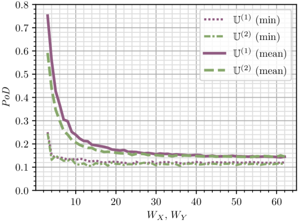
Figure 2: Price of Dishonesty (minimum and mean) guaranteed by BOSCO depending on the number of choices $W_{X}=W_{Y}$ for two different utility distributions $\mathbb{U}^{(1)}$ and $\mathbb{U}^{(2)}$.

It remains to analyze how the choice sets should be constructed such that equilibria with a low Price of Dishonesty result. Surprisingly, we have found that random generation of such choice sets works reasonably well in practice. In particular, the choice set $V_{X}$ for any party $X$ can be constructed by sampling a high enough number of choices $v_{X}$ from the utility distribution $\mathbb{U}_{X}$. With multiple trials of such random choice-set generation, choice sets with a relatively low Price of Dishonesty can be found.

In Fig. 2, for example, we analyze the resulting $\mathit{PoD}$ from random choice-set generation for two uniform utility distributions, namely $\mathbb{U}^{(1)}$, which is a uniform distribution of $(u_{X},u_{Y})$ on $[-1,1]\times[-1,1]$, and $\mathbb{U}^{(2)}$, which is a uniform distribution on $[-\frac{1}{2},1]\times[-\frac{1}{2},1]$. For each choice-set cardinality $W_{X}=W_{Y}$, we generate 200 random choice-set combinations and find the mean and the minimum of the associated $\mathit{PoD}$ values. Clearly, a higher number of choices generally helps to reduce the Price of Dishonesty, but given around 50 choices, adding more choices does not improve the mechanism efficiency. Interestingly, we also observe that the number of equilibrium choices (i.e., choices which have a non-empty associated interval in the equilibrium strategy) for each party reaches 4 at that point and is not further increased for more possible choices. Hence, the BOSCO service can increase the number of possible choices until the resulting $\mathit{PoD}$ values do not substantially decrease anymore. With this procedure, the BOSCO mechanism could guarantee a Price of Dishonesty of around 10% for both $\mathbb{U}^{(1)}$ and $\mathbb{U}^{(2)}$ in the example at hand, meaning that the negotiation can be expected to be 10% less efficient than under the unrealistic assumption of perfect honesty.

VI Effect on Path Diversity

In this section, we attempt to quantify the effect of mutuality-based agreements on path diversity in the Internet. Starting from the CAIDA AS-relationship dataset [8], we construct a network of ASes where a provider–customer or peering relationship results in a single provider–customer or peering link, respectively. In this graph, we generate all possible mutuality-based agreements (MAs) for the whole topology: For every pair $(A,B)$ of peers, we generate an MA in which $A$ gives $B$ access to all its providers and peers which are not customers of $B$, and vice versa. As MAs consist of an AS $A$ giving its peer $B$ access to a provider or another peer, these agreements enlarge the set of paths with 3 AS hops and 2 inter-AS links (henceforth: length-3 paths) for $B$, as well as the set of ASes that $B$ can reach with such length-3 paths (henceforth: nearby destinations).

Given this graph and these MAs, we perform the following analysis for 500 randomly chosen ASes. First, we find the GRC-conforming length-3 paths starting at the given AS. Then, we find the MA-created length-3 paths for which the given AS is an end-point. The number of these additional paths and the number of additional nearby destinations are thus metrics for the increased path diversity that the given AS enjoys thanks to MAs.

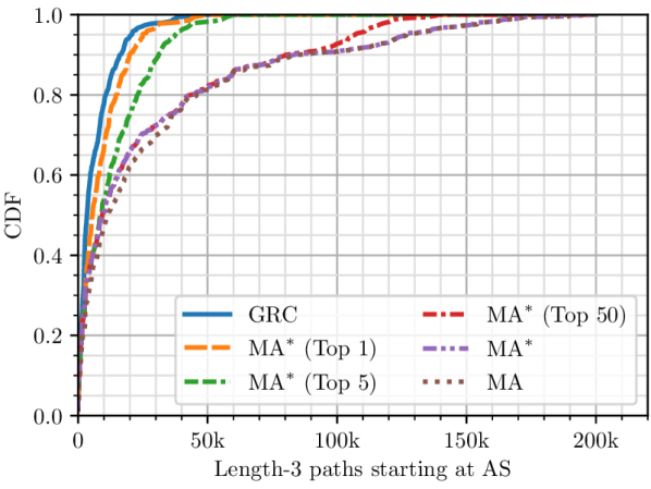
Figure 3: Distribution of ASes with respect to the number of length-3 paths starting at the AS, given different degrees of MA conclusion.

VI-A Number of Paths and Nearby Destinations

Figure 3 shows the substantial increase in the number of length-3 paths with that are potentially available to these ASes thanks to mutuality-based agreements: For example, whereas none of the analyzed ASes have more than 45,000 GRC-conforming paths with length 3, 20% of the analyzed ASes have more than 45,000 length-3 paths if all MAs are concluded (CDF for ’MA’). Note that for a fixed source and a fixed destination, all length-3 paths are disjoint by definition.

Since the conclusion of all possible MAs is an extreme case (although MAs could be negotiated in an automated fashion with the mechanism presented in § V), we further analyze the effects of non-comprehensive agreement conclusion. Initially, we note that an MA can provide an AS with new paths in two manners. First, an AS can directly gain an MA path by concluding an MA that includes the path (e.g., as AS $D$ gains the path $DEB$ in Fig. 1 from the MA with AS $E$). Second, an AS can indirectly gain an MA path by being the subject of an MA that includes the path (e.g., as AS $B$ or AS $F$ gain paths to AS $D$ from the MA between AS $D$ and AS $E$ in Fig. 1). Interestingly, most additional MA paths are directly gained paths, as the similarity of the CDFs for all MA paths (MA) and directly gained MA paths ($\mathrm{MA}^{\ast}$) in Fig. 3 suggests. Hence, the ASes bearing the negotiation effort of an MA have a strong incentive to negotiate that MA despite the effort, because they typically are its biggest beneficiaries. Moreover, we find that an AS already tends to obtain substantial gains in path diversity with only a handful of MAs. This point is demonstrated by the results for the scenarios where an AS only concludes the $n$ MAs which provide it with the most new paths (annotated with ‘$\mathrm{MA}^{\ast}$ (Top $n$)’ in Fig. 3): Even if an AS only concludes the single most attractive agreement from its perspective, it stands to gain several thousands of new paths.

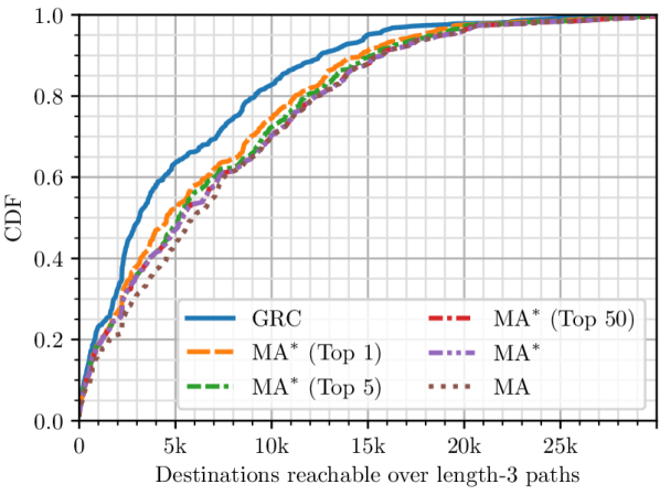
Figure 4: Distribution of ASes with respect to the number of destination reachable over length-3 paths, given different degrees of MA conclusion.

Figure 4 also illustrates that mutuality-based agreements enlarge the set of destinations reachable with paths of length 3: For example, whereas 40% of the analyzed ASes can reach more than 5,000 destinations over length-3 paths, 57% of ASes can reach more than 5,000 destinations over such paths if all MAs are concluded. Interestingly, very few MAs per AS already suffice to reap most of these benefits, as the results for non-comprehensive agreement conclusion demonstrate.

For the set of analyzed ASes, the average number of additional length-3 paths thanks to mutuality-based agreements is 22,891 paths (maximum: 196,796 paths), and the average number of additionally reachable destinations over length-3 paths is 2,181 ASes (maximum: 7,144 ASes). Interestingly, the gains in terms of additionally reachable destinations are more broadly distributed than the gains regarding paths. The explanation for this phenomenon is that mutuality-based agreements in very densely connected regions of the Internet lead to a high number of additional length-3 paths, but have little impact on the number of ASes reachable over such paths.

VI-B Geodistance

In order to gain a more qualitative perspective on the additional paths enabled by MAs, we also investigate the geographical length (henceforth: geodistance) of these new paths. Such geodistance is an important determinant of path latency [49], which is typically considered a core aspect of path diversity. As the CAIDA AS-relationship dataset [8] does not directly contain the necessary information, we additionally build on the CAIDA prefix-to-AS dataset [9], the GeoLite2 database [32], and the CAIDA geographic AS-relationship dataset [7]. In particular, we determine the geolocation of any AS by finding the IP prefixes associated with the AS number in the prefix-to-AS dataset, determining the geolocation of the IP prefixes via the GeoLite2 database, and averaging the resulting coordinates to obtain the center of gravity of the AS. With such averaging, the potentially considerable intra-AS latency of geographically distributed top-tier ASes is automatically taken into account. Moreover, we obtain the geolocation of an AS interconnection from the CAIDA geographic AS-relationship dataset. The geodistance of a length-3 path $\pi=(A_{1},\ell_{12},A_{2},\ell_{23},A_{3})$, where $A_{i}$ are ASes and $\ell_{j}$ are inter-AS links, is then computed as $d(\pi)=d(A_{1},\ell_{12})+d(\ell_{12},\ell_{23})+d(\ell_{23},A_{3})$, where $d(X,Y)$ is the geodistance between two points. If there are multiple known AS interconnections, the geodistance of the AS-level path $(A_{1},A_{2},A_{3})$ is computed for $\ell_{12}$ and $\ell_{23}$ that minimize $d(\pi)$.

Using this measure of path geodistance, we again compare the set of paths that conform to the GRC and the set of paths enabled by novel MAs. For every analyzed AS pair connected by at least one length-3 GRC path, we determine the maximum, median, and minimum geodistance given the length-3 GRC paths connecting the AS pair. In a next step, we determine the geodistance of the additional MA paths and check for each MA path whether it is lower than the maximum, median, or minimum GRC geodistance, respectively. Each AS pair is then characterized by the number of MA paths below these comparison thresholds. The aggregate results of this comparison method are presented in Fig. 5(a).

Figure 5(a) shows that through MAs, around 50% of AS pairs gain at least 1 path with a lower geodistance than the minimum-geodistance GRC path, suggesting that inter-AS latency can be decreased by MAs in these cases. Around 25% of AS pairs even gain at least 5 paths that improve upon the minimum GRC geodistance, and at least 7 and 8 paths that improve upon the median and maximum GRC geodistance, respectively. Another 20% of AS pairs only gain MA paths with a higher geodistance than the maximum GRC geodistance (or no new paths at all); however, also these additional paths have value in terms of reliability. Regarding the AS pairs experiencing a reduction in minimum geodistance, Fig. 5(b) illustrates the considerable extent of the geodistance reduction for these AS pairs: For example, 50% of AS pairs that experience a geodistance reduction obtain a reduction of more than 24%.

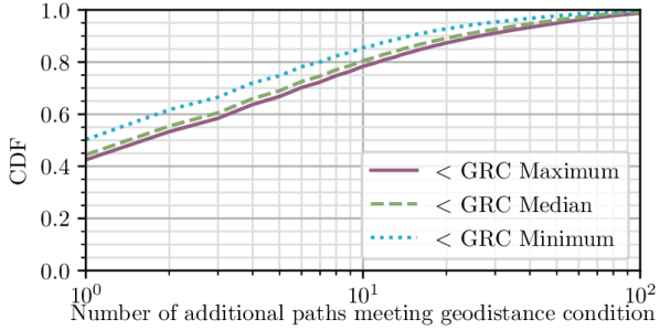
(a) Distribution of AS pairs with respect to geographical length of additional paths from mutuality-based agreements, distinguished by satisfied geodistance-comparison condition.

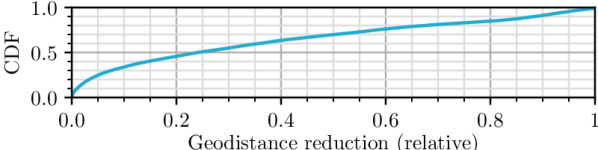
(b) Distribution of relevant AS pairs (i.e., AS pairs which experience a geodistance reduction thanks to MAs) with respect to the relative geodistance reduction from mutuality-based agreements.

Figure 5: Results of geodistance analysis.

VI-C Bandwidth

We perform an analogous analysis as in the preceding section with respect to the bandwidth of additional paths. To infer the bandwidth of inter-AS links, we employ a degree-gravity model [47] which endows each link with a capacity value proportional to the product of the node degrees of the link end-points. The path bandwidth is then the minimum such computed link bandwidth of all links in the path.

With such an analysis, we find that 35% of all investigated AS pairs obtain a new MA path that has more bandwidth than the corresponding maximum-bandwidth GRC path (cf. Fig. 6(a)). Of these benefiting AS pairs, 50% gain an MA path with at least 150% more bandwidth than the respective maximum-bandwidth GRC path (cf. Fig. 6(b)).

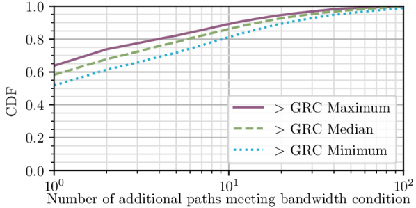
(a) Distribution of AS pairs with respect to bandwidth of additional paths from mutuality-based agreements, distinguished by satisfied bandwidth-comparison condition.

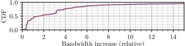
(b) Distribution of relevant AS pairs (i.e., AS pairs which experience a bandwidth increase thanks to MAs) with respect to the relative bandwidth increase from mutuality-based agreements.

Figure 6: Results of bandwidth analysis.

VII Related Work

After the growth of the Internet had led to considerable BGP stability problems in the late 1990s [21, 30], the research of AS interconnection agreements, their stability properties, and their optimal structures received significant interest. The commercial reality of the Internet has been shown to mainly contain two basic types of agreements that determine route-forwarding policies, namely provider–customer agreements and peering agreements [28, 41]. The relative exclusiveness of these two agreement types was reinforced by the important result of Gao and Rexford, showing that BGP route convergence is guaranteed if ASes stick to these two forms of route-forwarding policies [16].

However, it is well-known that such strict BGP policies reduce path quality: For a majority of routes selected in BGP, there exists a route that is more attractive with respect to metrics such as bandwidth, latency, or loss rate [48, 29, 26, 19, 17, 43]. In fact, motivated by such improvements, already today, many ASes do not always follow the Gao–Rexford conditions [17]. For example, some ISPs use alternative paths to reach content distribution networks such as Akamai [3, 33, 18], other ISPs prefer the peer route through their Tier-1 neighbor over a longer customer route [3], and so on. Still, these deviations are narrow in scope, with most non-GRC policies being explainable by “sibling” ASes, which belong to the same organization and provide mutual transit services [15, 3], and partial/hybrid provider relationships [18]. This is due to the fact that more complex policies would threaten the convergence of the routing process unless they are supported through multi-AS coordination efforts. These restrictions have also been acknowledged by previous efforts to provide multipath routing based on BGP such as MIRO [53].

While interconnection agreements in PAN architectures [44, 45, 4, 54, 20, 2, 56, 42, 51] do not need to follow the guidelines devised to achieve BGP stability, these agreements should definitely also respect the economic self-interest of ASes. The Gao–Rexford guidelines for BGP policies have been proven to be rational in that sense [14]. Notable proposals for agreement structures that attempt to satisfy both AS self-interest and global efficiency include Nash peering [13, 55], where the cooperative surplus of the agreement is shared among the parties according to the Nash bargaining solution [39], and ISP-settlement mechanisms based on the Shapley value [31]. It is important to note that unlike traditional source routing and similar to MIRO [53], PANs still offer transit ASes control over the traffic traversing their network, and hence to maximize their revenue. In contrast to MIRO, however, PANs guarantee path stability.

Finally, our paper has parallels to the work by Haxell and Wilfong [27], who showed that a fractional relaxation of the stable-paths problem of BGP [23] guarantees a solution and that a more flexible routing paradigm can thus defuse BGP stability issues. In contrast to this work, however, our focus lies on the interconnection agreements under this new paradigm, the extent to which these agreements increase path diversity, and their economic rationality and bargaining aspects.

VIII Conclusion

This work shows that PAN architectures enable novel types of interconnection agreements, thereby substantially improving path diversity in the Internet and creating new business opportunities. Such new possibilities exist in PAN architectures as they do not rely on the nowadays essential route-forwarding policy guidelines formulated by Gao and Rexford [16] for route convergence.

Our results show that path diversity in the Internet benefits enormously by enabling paths beyond the Gao–Rexford constraints: By using previously impossible path types, an AS can reach thousands of new destinations with 3-hop paths and benefit from hundreds of thousands of additional paths, some of which have more desirable characteristics than the previously available paths. There is thus a largely unknown advantage to PAN architectures: Not only do these architectures enable end-hosts to select a forwarding path, they also allow network operators to offer new (and often shorter) forwarding paths. As PANs are not limited to using a single path between a pair of ASes, all these paths can be used simultaneously according to the requirements of end-hosts and their applications (e.g., low latency for voice over IP and high bandwidth for file transfers). These direct benefits to end-hosts in turn incentivize providers to explore new interconnection agreements and offer diverse paths to attract new customers.

We present two methods for designing agreements that are Pareto-optimal, fair, and thus attractive to both parties. We also show that, assisted by an appropriate bargaining mechanism, the negotiation of such agreements can lead to efficient agreements although necessary information is private.

We see this work merely as a first step in exploring the new possibilities for interconnection agreements in PAN architectures. There are many exciting opportunities for future research in designing and evaluating interconnection agreements that can achieve desirable goals of network operators, such as network utilization, predictability, and security.

IX Acknowledgments

We gratefully acknowledge support from ETH Zurich, from the Zurich Information Security and Privacy Center (ZISC), from SNSF for project ESCALATE (200021L_182005) and from WWTF for project WHATIF (ICT19-045, 2020-2024). Moreover, we thank Giacomo Giuliari and Joel Wanner for helpful discussions that improved this research.

References

- [1] Anapaya Systems. SCION-Internet: The new way to connect. https://www.anapaya.net/scion-the-new-way-to-connect.
- [2] T. Anderson, K. Birman, R. Broberg, M. Caesar, D. Comer, C. Cotton, M. J. Freedman, A. Haeberlen, Z. G. Ives, A. Krishnamurthy, W. Lehr, B. T. Loo, D. Mazières, A. Nicolosi, J. M. Smith, I. Stoica, R. van Renesse, M. Walfish, H. Weatherspoon, and C. S. Yoo. The NEBULA future Internet architecture. In The Future Internet. Springer, 2013.
- [3] R. Anwar, H. Niaz, D. Choffnes, Í. Cunha, P. Gill, and E. Katz-Bassett. Investigating interdomain routing policies in the wild. In Internet Measurement Conference (IMC), 2015.
- [4] B. Bhattacharjee, K. Calvert, J. Griffioen, N. Spring, and J. P. G. Sterbenz. Postmodern internetwork architecture. NSF Nets FIND Initiative, 2006.
- [5] K. Binmore, A. Rubinstein, and A. Wolinsky. The Nash bargaining solution in economic modelling. The RAND Journal of Economics, 1986.
- [6] K. L. Calvert, J. Griffioen, A. Nagurney, and T. Wolf. A vision for a spot market for interdomain connectivity. In 2019 IEEE 39th International Conference on Distributed Computing Systems (ICDCS), pages 1860–1867. IEEE, 2019.
- [7] Center for Applied Internet Data Analysis. The CAIDA AS relationships dataset with Geographic Annotations. https://data.caida.org/datasets/as-relationships-geo/, 2016.
- [8] Center for Applied Internet Data Analysis. The CAIDA AS relationships dataset. http://data.caida.org/datasets/as-relationships/serial-2/20200401.as-rel2.txt.bz2, 2020.
- [9] Center for Applied Internet Data Analysis. The CAIDA Routeviews Prefix-to-AS dataset. http://data.caida.org/datasets/routing/routeviews-prefix2as/, 2020.
- [10] L. Cittadini, G. Di Battista, T. Erlebach, M. Patrignani, and M. Rimondini. Assigning AS relationships to satisfy the Gao-Rexford conditions. In IEEE International Conference on Network Protocols, 2010.
- [11] E. H. Clarke. Multipart pricing of public goods. Public Choice, 11(1), 1971.
- [12] G. Debreu. Valuation equilibrium and Pareto optimum. US National Academy of Sciences, 1954.
- [13] A. Dhamdhere, C. Dovrolis, and P. Francois. A value-based framework for Internet peering agreements. In International Teletraffic Congress (ITC), 2010.
- [14] J. Feigenbaum, V. Ramachandran, and M. Schapira. Incentive-compatible interdomain routing. In ACM Conference on Electronic Commerce, 2006.
- [15] L. Gao. On inferring autonomous system relationships in the Internet. IEEE/ACM Transactions on Networking, 9(6), 2001.
- [16] L. Gao and J. Rexford. Stable Internet routing without global coordination. IEEE/ACM Transactions on Networking, 2001.
- [17] P. Gill, M. Schapira, and S. Goldberg. A survey of interdomain routing policies. ACM SIGCOMM Computer Communication Review (CCR), 44(1), 2013.
- [18] V. Giotsas, M. Luckie, B. Huffaker, and K. Claffy. Inferring complex AS relationships. In Internet Measurement Conference (IMC), 2014.
- [19] V. Giotsas, S. Zhou, M. Luckie, and K. Claffy. Inferring multilateral peering. In ACM Conference on Emerging Networking Experiments and Technologies (CoNEXT), 2013.
- [20] P. B. Godfrey, I. Ganichev, S. Shenker, and I. Stoica. Pathlet routing. ACM SIGCOMM Computer Communication Review (CCR), 2009.
- [21] R. Govindan and A. Reddy. An analysis of Internet inter-domain topology and route stability. In IEEE Conference on Computer Communications (INFOCOM), volume 2. IEEE, 1997.
- [22] T. Griffin and G. Huston. BGP wedgies. RFC 4264, IETF, 2005.
- [23] T. G. Griffin, F. B. Shepherd, and G. Wilfong. The stable paths problem and interdomain routing. IEEE/ACM Transactions on Networking, 10(2), 2002.
- [24] T. G. Griffin and G. Wilfong. An analysis of BGP convergence properties. ACM SIGCOMM Computer Communication Review (CCR), 29(4), 1999.
- [25] T. Groves. Incentives in teams. Econometrica: Journal of the Econometric Society, 1973.
- [26] A. Gupta, L. Vanbever, M. Shahbaz, S. P. Donovan, B. Schlinker, N. Feamster, J. Rexford, S. Shenker, R. Clark, and E. Katz-Bassett. SDX: A software defined Internet exchange. ACM SIGCOMM Computer Communication Review (CCR), 2015.
- [27] P. E. Haxell and G. T. Wilfong. A fractional model of the Border Gateway Protocol (BGP). In ACM-SIAM Symposium on Discrete Algorithms, USA, 2008. Society for Industrial and Applied Mathematics.
- [28] G. Huston. Interconnection, peering and settlements. The Internet Protocol Journal, 2(1), 1999.
- [29] V. Kotronis, R. Kloti, M. Rost, P. Georgopoulos, B. Ager, S. Schmid, and X. Dimitropoulos. Stitching inter-domain paths over IXPs. In Symposium on SDN Research (SOSR), 2016.
- [30] C. Labovitz, A. Ahuja, and F. Jahanian. Experimental study of Internet stability and backbone failures. In International Symposium on Fault-Tolerant Computing. IEEE, 1999.
- [31] R. T. Ma, D. M. Chiu, J. C. Lui, V. Misra, and D. Rubenstein. Internet economics: The use of Shapley value for ISP settlement. IEEE/ACM Transactions on Networking, 2010.
- [32] MaxMind. GeoLite2 Free Downloadable Databases. https://dev.maxmind.com/geoip/geoip2/geolite2/, 2020.
- [33] R. Mazloum, M.-O. Buob, J. Auge, B. Baynat, D. Rossi, and T. Friedman. Violation of interdomain routing assumptions. In International Conference on Passive and Active Network Measurement, 2014.
- [34] D. Monderer and L. S. Shapley. Potential games. Games and economic behavior, 14(1):124–143, 1996.
- [35] R. Müller, A. Perea, and S. Wolf. Weak monotonicity and Bayes–Nash incentive compatibility. Games and Economic Behavior, 61(2), 2007.
- [36] R. B. Myerson. Incentive compatibility and the bargaining problem. Econometrica: Journal of the Econometric Society, 1979.
- [37] R. B. Myerson and M. A. Satterthwaite. Efficient mechanisms for bilateral trading. Journal of Economic Theory, 29(2), 1983.
- [38] J. Nachbar. The Myerson-Satterthwaite theorem. Washington University, 2017.
- [39] J. F. Nash Jr. The bargaining problem. Econometrica: Journal of the Econometric Society, 1950.
- [40] S. Nath and T. Sandholm. Efficiency and budget balance in general quasi-linear domains. Games and Economic Behavior, 113, 2019.
- [41] W. B. Norton. The Internet peering playbook: connecting to the core of the Internet. DrPeering Press, 2011.
- [42] A. Perrig, P. Szalachowski, R. M. Reischuk, and L. Chuat. SCION: A Secure Internet Architecture. Springer, 2017.
- [43] S. Y. Qiu, P. D. McDaniel, and F. Monrose. Toward valley-free inter-domain routing. In IEEE International Conference on Communications. IEEE, 2007.
- [44] B. Raghavan and A. C. Snoeren. A system for authenticated policy-compliant routing. ACM SIGCOMM Computer Communication Review (CCR), 34(4), 2004.
- [45] B. Raghavan, P. Verkaik, and A. C. Snoeren. Secure and policy-compliant source routing. IEEE/ACM Transactions on Networking, 17(3), 2009.
- [46] T. Roughgarden. Intrinsic robustness of the price of anarchy. Journal of the ACM (JACM), 62(5), 2015.
- [47] L. Saino, C. Cocora, and G. Pavlou. A toolchain for simplifying network simulation setup. SimuTools, 13, 2013.
- [48] S. Savage, A. Collins, E. Hoffman, J. Snell, and T. Anderson. The end-to-end effects of Internet path selection. In ACM SIGCOMM Computer Communication Review (CCR), 1999.
- [49] A. Singla, B. Chandrasekaran, P. B. Godfrey, and B. Maggs. The Internet at the speed of light. In ACM Workshop on Hot Topics in Networks (HotNets), 2014.
- [50] Swisscom AG. Enhancing WAN connectivity and services for Swiss organisations with the next-generation internet. https://www.swisscom.ch/en/business/enterprise/downloads/security/international-connectivity-business.html.
- [51] B. Trammell, J.-P. Smith, and A. Perrig. Adding path awareness to the Internet architecture. IEEE Internet Computing, 2018.
- [52] W. Vickrey. Counterspeculation, auctions, and competitive sealed tenders. The Journal of Finance, 16(1), 1961.
- [53] W. Xu and J. Rexford. MIRO: multi-path interdomain routing. In Conference on Applications, Technologies, Architectures, and Protocols for Computer Communications, 2006.
- [54] X. Yang, D. Clark, and A. W. Berger. NIRA: A new inter-domain routing architecture. IEEE/ACM Transactions on Networking, 2007.
- [55] D. Zarchy, A. Dhamdhere, C. Dovrolis, and M. Schapira. Nash-peering: A new techno-economic framework for Internet interconnections. In INFOCOM Workshop, 2018.
- [56] L. Zhang, K. Fall, and D. Meyer. Report from the IAB workshop on routing and addressing. RFC 4984, IETF, 2007.
- [57] X. Zhang, H.-C. Hsiao, G. Hasker, H. Chan, A. Perrig, and D. Andersen. SCION: Scalability, control, and isolation on next-generation networks. In Proceedings of the IEEE Symposium on Security and Privacy, 2011.