Bounded Inputs Total Energy Shaping for Mechanical Systems

Abstract

Designing control systems with bounded input is a practical consideration since realizable physical systems are limited by the saturation of actuators. The actuators’ saturation degrades the performance of the control system, and in extreme cases, the stability of the closed-loop system may be lost. However, actuator saturation is typically neglected in the design of control systems, with compensation being made in the form of over-designing the actuator or by post-analyzing the resulting system to ensure acceptable performance. The bounded input control of fully actuated systems has been investigated in multiple studies, but it is not generalized for under actuated mechanical systems. This article proposes a systematic framework for finding the upper bound of control effort in underactuated systems, based on interconnection and the damping assignment passivity based control (IDA-PBC) approach. The proposed method also offers design variables for the control law to be tuned, considering the actuator’s limit. The major difficulty in finding the control input upper bounds is the velocity dependent kinetic energy related terms. Thus, the upper bound of velocity is computed using a suitable Lyapunov candidate as a function of closed-loop system parameters. The validity and application of the proposed method are investigated in detail through two benchmark systems.

I Introduction

Underactuated mechanical systems (UMS) are characterized by the fact that they have fewer actuators than their degrees of freedom (DOF). In other words, the size of the configuration space exceeds the size of the control input space [1]. Examples of such systems include, but not limited to, legged robots, swimming robots, flying robots, continuum robots, and gantry cranes as well as manipulator with structural flexiblity. Underactuated robots (URs) are expected to be more energy-efficient and lightweight than fully actuated counterparts while still provide the adequate dexterity without reducing the reachable configuration space [2]. While UMS have broad applications in different disciplines, due to the reduced control inputs, the traditional non-linear control methods are not directly applicable. The control of UMS has been investigated through several control methods including feedback linearization, sliding mode, backstepping, fuzzy control, and passivity-based control (PBC). Except for the PBC approach, none of the mentioned methods have succeeded to be generalized to the UMS.

The term PBC was initially introduced in [3] as a control approach to make the closed-loop system passive. The PBC of UMS was first presented in [4] as the extension of the energy-shaping plus damping injection technique of [5], which was proposed to solve state feedback set point regulation problems in fully actuated robotic systems. The essence of passivity-based control is energy shaping [6], which provides a natural procedure to shape the potential energy in the closed-loop Euler–Lagrange (EL) systems [7]. Energy shaping control treats the plant and its controller as energy-transformation devices. In the trajectory tracking of the mechanical systems, the energy shaping control based on the classical procedure of PBC does not provide an EL representation of the closed-loop system, in other words, the total energy of the closed-loop is not a physical energy equation. Additionally, it cannot be used for stabilization of UMS as it is not suitable for total energy shaping and is mostly used for potential energy shaping. Nevertheless, an extended approach introduced in [7] as Interconnection and damping assignment passivity based control (IDA-PCB) offers a physically inspired generalized method for the control of UMS, in terms of solvability of two PDEs that correspond to the potential and kinetic energy shaping. By using this method, the dynamics of a mechanical system is expressed in the form of the Port Hamiltonian (PH) model with desired interconnection and damping matrices and a Hamiltonian function, which is the summation of desired potential and kinetic energy.

One of the most challenging aspects of the IDA-PBC is the analytical solution of the PDEs, which have been studied in various studies [8, 9, 10]. Moreover, the bounded input stabilization of UMS in the presence of input saturation is another challenging but importany issue that is rarely addressed. The concept of bounded input control applies to a wide variety of control applications. It is due to the fact that control inputs of realizable systems are constrained by the saturation of the actuator. Saturation of the actuator degrades the performance of the control systems and can lead to instability in the closed loop [11]. A common drawback seen in many of the control methods is the large magnitudes for the input torque, which, in fact, is not taken into account in the design procedure of the controller [12]. Actuator saturation is typically neglected in the design of control systems, with compensation being made in the form of over-designing of the actuator or by post-analyzing the resulting system to ensure acceptable performance.

In contrast to fully actuated robots, the bounded input stabilization of URs is less attended by the researchers. To the best of the authors’ knowledge, [13] is the only reported paper in the field of IDA-PBC approach, which is used for an inertia wheel pendulum that has bounded inputs. In this article, the system has a constant mass matrix, leading to the total energy being manipulated by a constant inertia matrix. By this means all terms related to kinetic energy shaping are cancelled. However, generally the mass matrix is configuration dependant and the kinetic energy terms appears in the energy shaping formulation. As the kinetic energy is quadratic with respect to velocity, the upper bound of energy cannot be simply calculated if the upper bound of the velocity is not known. In this article we present a generalized methodology to calculate the upper bound of the control input in UMS based on IDA-PBC. The proposed framework also provides design parameters to be tuned to restrict the control effort within the actuator saturation. To this aim, the upper bounds of the velocity terms in the control law are derived to find the maximum kinetic energy of the closed-loop system.

The IDA-PCB control law requires solving two PDEs, which in general have numerous solutions. In some conditions, the solution of PDEs which appears in the control law is non-smooth. Considering this, finding the upper bound of the IDA-PBC control law with the proposed framework allows using a suitable solution of the PDEs for the formulation of the control law, in order to keep the control effort within an expected limit. This application of the proposed method is further investigated through an example for which two solutions for the corresponding PDEs are found. Additionally we propose a two-phase control methodology for non-smooth control laws, in which a primary controller brings the state of the system into a region far from the singular points, and then the secondary controller is designed and implemented based on IDA-PBC.

The remaining structure of this paper is as follows; in Section II, we present an overview of the IDA-PBC for the ease of reference. Next, in Section III, we discuss a methodology to find the upper bound of the control input based on IDA-PBC approach. This is done by the analysis of every single terms of the control law, the potential energy related terms and kinetic energy related terms. Finally, in Section IV the applicability of the method is investigated in two separate case studies.

Notation. Unless determined, the vectors in this paper are column vector including the gradient of functions. For an arbitrary matrix $\xi\in\mathbb{R}^{n\times m}$ and vector $a\in\mathbb{R}^{n}$, $\xi_{i}$ and $a_{i}$ denotes the $i$th row and $i$th element of $\xi$ and $a$, respectively, $\xi_{(i,j)}$ is the $(i,j)$th element of that matrix, $I_{n}$ denotes an $n\times n$ identity matrix and $0_{m\times n}$ is an $m\times n$ matrix of zeros. Furthermore, $\mathbb{R}^{+}$ and $\mathbb{R}^{-}$ denote the set of positive and negative real numbers, and $\lambda_{m}\{\xi\}$ and $\lambda_{M}\{\xi\}$ denote the maximum and minimum eigenvalues of the square matrix $\xi$, respectively.

II IDA-PBC for Mechanical Systems with Physical Damping

For the ease of reference, a brief review of IDA-PBC for mechanical systems in the presence of natural damping (frictional forces) based on [14] is given here. The dynamic equations of a mechanical system with physical damping in the port Hamiltonian representation is as follow:

$$\begin{bmatrix}\dot{q}\\ \dot{p}\end{bmatrix}=\begin{bmatrix}0_{n\times n}&I_{n}\\ -I_{n}&-R(q)\end{bmatrix}\begin{bmatrix}\nabla_{q}H\\ \nabla_{p}H\end{bmatrix}+\begin{bmatrix}0_{n\times m}\\ G(q)\end{bmatrix}\tau$$ (1)

in which $n$ is the DOF and $m$ is the number of control inputs, $q,p\in\mathbb{R}^{n}$ are generalized position and momentum, respectively, and $M\dot{q}=p$, in which $M^{T}(q)=M(q)>0$ is the inertia matrix. Moreover, $H(q,p)=\frac{1}{2}p^{T}M^{-1}(q)p+V(q)$ is the total energy of the mechanical system which is the summation of the kinetic and potential energy, $G(q)\in\mathbb{R}^{n\times m}$ is the input coupling matrix and $R(q)\in\mathbb{R}^{n\times n}$ is the smooth positive semi-definite damping matrix. In IDA-PBC it is assumed that the desired structure of the closed-loop system is as follows:

$$\begin{bmatrix}\dot{q}\\ \dot{p}\end{bmatrix}=\begin{bmatrix}0_{n\times n}&M^{-1}M_{d}\\ -M_{d}M^{-1}&J_{2}-R_{2}\end{bmatrix}\begin{bmatrix}\nabla_{q}H_{d}\\ \nabla_{p}H_{d}\end{bmatrix}$$ (2)

where $M_{d}$ and $H_{d}$ are the desired mass matrix and the desired total energy of the closed loop system, respectively. Additionally $J_{2}(q,p)$ is a skew-symmetric matrix and $R_{2}$ is a positive semi-difinite matrix in the following form:

$$R_{2}=\frac{1}{2}(RM^{-1}M_{d}+M_{d}M^{-1}R)+GK_{v}G^{T}.$$ (3)

the desired equilibrium point $q^{*}$ should also satisfy:

$$q^{*}=\text{arg min}V_{d}(q).$$ (4)

Notice that in the rest of the paper, we assume that $V_{d}$ is designed such that at the desired equilibrium point $(q^{*})$, $H_{d}=0$. The control law proposed in the IDA-PBC method is defined as (II) which is obtained by setting (1) and (2) equal.

$$\tau=(G^{T}G)^{-1}G^{T}\bigg{(}\nabla_{q}V-M_{d}M^{-1}\nabla_{q}V_{d}+\nabla_{q}K$$

$$-M_{d}M^{-1}\nabla_{q}K_{d}+(J_{2}-GK_{v}G^{T})\nabla_{p}H_{d}\bigg{)}$$ (5)

The above mentioned control law requires $M_{d}$ and $V_{d}$ which are to be obtained through analytical solution of (6a) and (6b), respectively, given as below:

$$G^{\bot}(q)\{\nabla_{q}\big{(}p^{T}M^{-1}(q)p\big{)}-M_{d}M^{-1}(q)\nabla_{q}\big{(}p^{T}M_{d}^{-1}(q)p\big{)}+2J_{2}M_{d}^{-1}p\}=0_{s\times 1},$$ (6a)

$$G^{\bot}(q)\{\nabla_{q}V(q)-M_{d}M^{-1}\nabla_{q}V_{d}(q)\}=0_{s\times 1},$$ (6b)

in which $s=n-m$ and $G^{\bot}$ is the left annihilator of $G$. Note that, in the presence of physical damping in the model, there would be one extra PDE, however, it will be removed with damping injection [14], by suitably selecting $K_{v}$. It is to be noted that the analytical solution of the PDEs in (6) requires extensive calculation, for which the detailed description can be found in [15, 16]. Considering $H_{d}$ as the desired Lyapunov function of the closed loop system, its derivative will be:

$$\dot{H}_{d}=-p^{T}M_{d}^{-1}R_{2}M_{d}^{-1}p,$$

which is generally negative semi-definite. Thus the desired equilibrium point is stable. Equilibrium point is asymptotically stable if it is locally detectable from $G^{T}M_{d}^{-1}p$, in other words if $G^{T}M_{d}^{-1}p=0$. Note that if the following condition holds

$$G^{\bot}(RM^{-1}M_{d}+M_{d}M^{-1}R)(G^{\bot})^{T}>0,$$ (7)

then $R_{2}$ is positive definite.

III Bounded Input IDA-PBC for Mechanical Systems

In this section, having the parameters of the control law (II), we propose a methodology to find the upper bound of the control law. First the upper bound of the potential energy terms is obtained by suitably choosing the homogeneous solution of $V_{d}$. Next, to find the upper bound of the kinetic energy, the upper bounds of the velocity is found in Theorem 1. Finally the upper bound of the control law is obtained by adding up the upper bound of the kinetic and potential energy related terms.

With a minor loss of generality, first assume that the elements of the matrix $G$ are merely 0 or 1. The solution of the potential energy PDE (6b) may be separated by two terms as the following:

$$V_{d}=V_{dn}+V_{dh},$$

in which, $V_{dn}$ and $V_{dh}$ denote the non-homogeneous and homogeneous solution of the potential energy PDE, respectively. The homogeneous solution is given by:

$$G^{\bot}M_{d}M^{-1}\nabla_{q}V_{dh}(q)=0,$$

which may be represented as follows [17, ch. 2]

$$V_{dh}=\Phi\big{(}V_{dh_{1}},V_{dh_{2}},\dots\big{)}$$

where $\Phi$ is an arbitrary function and $V_{dh_{i}}$’s are the solutions of the homogeneous equation. The function $\Phi$ usually is chosen in quadratic form to satisfy (4). However, this may lead to unbounded control law. Thus, we propose an alternative function for $\Phi$ in order to make the bounded control law. Invoking [18], this issue maybe is rectified by defining $V_{dh}$ as follows

$$V_{dh}=\displaystyle\sum k_{i}\int\mathcal{S}(V_{dh_{i}}-V_{dh_{i}}^{*})dV_{dh_{i}}$$ (8)

in which, $V_{dh_{i}}^{*}=\left.V_{dh_{i}}\right|_{q=q^{*}}$ and the function $\mathcal{S}(x)$ should satisfy the following properties

• $\mathcal{S}(0)=0$,

• $\mathcal{S}$ is an increasing function such that $|\mathcal{S}|\leq 1$,

• $\frac{d^{2}\mathcal{S}(x)}{dx^{2}}\neq 0,\qquad\forall x\neq 0$.

As an example, $S(x)=\tanh(x)$ satisfies these three conditions. Generally, the control law of UMS might be unbounded, based on the physics of the problem, as explained in Brockett’s theorem (e.g. when in cart-pole system the position of the swinging arm is horizontal). In this situation regardless of the selection of $S(x)$ the functions $V_{dh}$ and $V_{dn}$ could be non-smooth. Being such, the following assumption is essential for development of the rest of the paper (see Remark 3 to see how this assumption is relaxed).

Assumption 1

Consider the dynamic model of a mechanical system in the form (1). Assume that the input coupling matrix is in the form $G=P[I_{m},0_{s\times m}]^{T}$ with $P$ being a permutation matrix. The coefficients $k_{i}$s in (8) shall be sufficiently small. Considering the potential energy terms of the control law ($(\nabla_{q}V-M_{d}M^{-1}\nabla_{q}V_{d})_{i}$), the upper bounds of the actuators should satisfy the following inequality:

$$|(\nabla_{q}V-M_{d}M^{-1}\nabla_{q}V_{d})_{i}|<\tau_{i_{max}}$$ (9)

meaning that the control law should be able to compensate the effects of gravitational force in the entire workspace. In the above equation $(\cdot)_{i}$ denotes the $i$th element of $(\cdot)$ while $i$ counts merely for the actuated joints. In other words, $\nabla_{q}V$ and $\nabla_{q}V_{d}$ are bounded as follow:

$$\|(\nabla_{q}V)_{i}\|\leq c_{V_{i}},\qquad\|\nabla_{q}V_{d}\|\leq c_{V_{d}}.$$ (10)

$\Box$

Additionally for the kinetic energy terms of the control law ($\nabla_{q}K-M_{d}M^{-1}\nabla_{q}K_{d}$), as $K=1/2p^{T}M^{-1}p$ and $K_{d}=1/2p^{T}M_{d}^{-1}p$, it is clear that the kinetic energy terms are quadratic functions of $p$. Hence, restricting the velocity may result in the restriction of kinetic energy shaping terms in the control law. Before presenting the main results, we also need the following assumption.

Assumption 2

It is assumed that there are constants $c_{M}$, $c_{M_{d}},c_{J}$ and $c_{\Lambda_{i}}$ satisfying:

$$(\nabla_{q}K)_{i}\leq c_{M_{i}}\|p\|^{2},\hskip 5.69054pt\nabla_{q}K_{d}\leq c_{M_{d}}\|p\|^{2},\hskip 5.69054pt\|J_{2}(q,p)\|\leq c_{J}\|\tilde{p}\|,\hskip 5.69054pt\|\Lambda_{i}\|\leq c_{\Lambda_{i}}$$ (11)

with $\Lambda:=M_{d}M^{-1}$. $\Box$

In the following theorem, the upper bounds of both $\|p\|$ and control law are found. Note that the previously mentioned assumption $G=P[I_{m},0_{s\times m}]^{T}$ is relaxed in Remark 2.

Theorem 1

Consider a mechanical system with the dynamic model (1) and control law (II). Presume that conditions (7), Assumption 1 and Assumption 2 are satisfied, thus:

• The upper bound of $\|p\|$ and $\|\tilde{p}\|$ are as follows:

  $$\|p\|\leq\sqrt{\frac{H_{d}(t_{0})}{\lambda_{m}\{M_{d}^{-1}\}}}=c_{p1},\quad\|\tilde{p}\|\leq\sqrt{\frac{H_{d}(t_{0})}{\lambda_{m}\{M_{d}\}}}=c_{\tilde{p}1},$$ (12)

  where $\tilde{p}=M_{d}^{-1}p$.

• The ultimate bound of $\|p\|$ and $\|\tilde{p}\|$ are given by:

  $$\|p\|\leq\Big{(}\dfrac{\lambda_{M}\{M_{d}^{-1}\}}{\lambda_{m}\{M_{d}^{-1}\}}\Big{)}^{1/2}\frac{c_{V_{d}}\lambda_{M}\{M_{d}^{-1}\}}{\lambda_{m}^{2}\{M_{d}^{-1}\}\lambda_{m}\{R_{2}\}+\mu}=c_{p2}.$$ (13a)

  $$\|\tilde{p}\|\leq\Big{(}\dfrac{\lambda_{M}\{M_{d}\}}{\lambda_{m}\{M_{d}\}}\Big{)}^{1/2}\frac{c_{V_{d}}}{\lambda_{m}\{R_{2}\}+\mu}=c_{\tilde{p}2},$$ (13b)

  in which $$\lambda_{m}\{\cdot\} \lambda_{M}\{\cdot\} \{\cdot\}$$ and denote the maximum and the minimum eigenvalue of , respectively.

• The upper bound of $|\tau_{i}|$ is:

  $$c_{V_{i}}+c_{\Lambda_{i}}c_{V_{d}}+\big{(}c_{M_{i}}+c_{\Lambda_{i}}c_{M_{d}}\big{)}c_{p}^{2}+c_{J}c_{\tilde{p}}^{2}+\lambda_{M}\{K_{v}\}c_{\tilde{p}},$$ (14)

  where $c_{p}$ and $c_{\tilde{p}}$ denote the upper bound of $\|p\|$ and $\|\tilde{p}\|$ respectively. Generally, $c_{p}=c_{p1}$ and $c_{\tilde{p}}=c_{\tilde{p}1}$, but if $\|p(t_{0})\|\leq c_{p2}$ and $\|\tilde{p}(t_{0})\|\leq c_{\tilde{p}2}$, then

  $$c_{p}=\min\{c_{p1},c_{p2}\},\qquad c_{\tilde{p}}=\min\{c_{\tilde{p}1},c_{\tilde{p}2}\}.$$

  $\Box$

Proof. a) Consider $H_{d}$ as a Lyapunov candidate. Since the time derivative of $H_{d}$ is negative semi-definite, the system’s trajectory that starts from $H_{d}(t_{0})$ descends to lower level sets. In other words, we have the following inequality.

$$\frac{1}{2}\lambda_{m}\{M_{d}\}\|\tilde{p}\|^{2}\hskip 5.69054pt\&\hskip 5.69054pt\frac{1}{2}\lambda_{m}\{M_{d}^{-1}\}\|p\|^{2}\leq K_{d}\leq H_{d}\leq H_{d}(t_{0}).$$

Hence, the upper bounds of $|\tilde{p}\|$ and $\|p\|$ are derived easily.

b) Consider the desired kinetic energy as a Lyapunov candidate:

$$K_{d}=H_{d}-V_{d},$$ (15)

and its time derivative as:

$$\dot{K}_{d} =-p^{T}M_{d}^{-1}R_{2}M_{d}^{-1}p-(\nabla_{q}V_{d})^{T}M_{d}^{-1}p$$

$$\leq-\|p\|^{2}\lambda_{m}^{2}\{M_{d}^{-1}\}\lambda_{m}\{R_{2}\}+\|\nabla_{q}V_{d}\|\lambda_{M}\{M_{d}^{-1}\}\|p\|.$$ (16)

This inequality assures that $\|p\|$ is bounded since the negative part is proportional to $\|p\|^{2}$ while the other term is proportional to $\|p\|$. In order to derive the upper bound of $\|p\|$, Theorem 4.18 of [19] is utilized. It is clear that Lyapunov candidate (15) is within the following bounds

$$\frac{1}{2}\lambda_{m}\{M_{d}^{-1}\}\|p\|^{2}\leq K_{d}\leq\frac{1}{2}\lambda_{M}\{M_{d}^{-1}\}\|p\|^{2}.$$

On the other hands, the right hand side of (III) is less than $-\mu\|p\|^{2}$ if:

$$\|p\|\geq\frac{c_{V_{d}}\lambda_{M}\{M_{d}^{-1}\}}{\lambda_{m}^{2}\{M_{d}^{-1}\}\lambda_{m}\{R_{2}\}+\mu},$$

where $\mu\in\mathbb{R}^{+}$ is an arbitrary value, while Assumption 1 is used for the upper bound of $\nabla_{q}V_{d}$. The final ultimate bound for $\|p\|$ is derived as (13a). With a similar approach, the ultimate bound of $\tilde{p}$ can be found . Note that it is possible to compute upper bound of $\tilde{p}$ based on (13a), however it is a more conservative choice than (13b). From (13a) and (13b), it is clear that the ultimate bound of velocity can be reduced by increasing $\lambda_{m}\{R_{2}\}$. Notice that these ultimate bounds are also the upper bounds if the initial condition of $p$ and $\tilde{p}$ are less than $c_{p2}$ and $c_{\tilde{p}2}$, respectively.

c) Based on Assumption 2, the upper bound for $i$th element of the kinetic energy shaping terms is:

$$\big{(}c_{M_{i}}+c_{\Lambda_{i}}c_{M_{d}}\big{)}c_{p}^{2}$$ (17)

in which the parameters was defined in the Assumption 2. Note that as explained in [16], $J_{2}$ should be linear with respect to velocity. Hence, it can be represented as

$$J_{2}(q,p)=\displaystyle\sum_{i=1}^{n_{0}}\tilde{p}^{T}\alpha_{i}(q)W_{i}$$

where $n_{0}=\frac{n(n-1)}{2}$, and $W_{i}$s are skew-symmetric constant matrices. Since $\alpha_{i}$s are determined based on PDE (6a), we infer that:

$$\|J_{2}(q,p)\|\leq c_{J}\|\tilde{p}\|$$ (18)

Thus, $J_{2}\tilde{p}$ has also an upper bound proportional to $\|\tilde{p}\|^{2}$. Now the damping term in (II) is analyzed for which the upper bound is given by:

$$\|K_{v}G^{T}\tilde{p}\|\leq\lambda_{M}\{K_{v}\}c_{\tilde{p}}.$$ (19)

Finally, the upper bound of $i$th element of control law (II) is derived simply by adding the above terms obtained in (19),(17),(18),(11) and (10) as (14).

 

Remark 1

The natural damping of the system represented by $R$ is configuration independent, whether it is actuated or not, thus $R$ may be considered positive definite. If the natural damping is considered in the modeling, condition (7) is certainly satisfied. On the other hand, if it is not modeled such, or if (7) is not satisfied, part $b$ of the Theorem 1 is not applicable. As explained earlier, the proposed method finds two upper bounds for the velocity. For the model with no natural damping term, the upper bound of the velocity is obtained from part $a$ of the Theorem 1. On the other hand, if the natural damping is included in the model and $R_{2}$ is positive definite, the bound of the velocity will be the minimum of the two upper bounds obtained in parts $a$ and $b$ of the Theorem 1. $\Box$

In some UMS like the parallel robot in [20] and VTOL aircraft [16], the input coupling matrix $G(q)$ is configuration-dependent. Furthermore, the bound of the control input is not necessarily symmetric ($\tau_{min}\neq-\tau_{max}$), e.g., in cable-driven robots, the control input $\tau$ should be positive as the cables merely apply tensile forces [21]. In the following remark, these issues are addressed.

Remark 2

Let $G(q)$ be a full rank matrix that maps the actuator forces/torques to configuration space force/torque of the robot. Hence, without loss of generality, as it is configuration dependant, it is bounded in the entire workspace of the robot. Assume that,

$$\|(G^{T}G)^{-1}G^{T}\|\leq G_{M},\qquad\|G\|\leq G_{m}.$$

In this case, the upper bound for the control law will be given by

$$G_{M}\big{(}c_{V_{i}}+c_{\Lambda_{i}}c_{V_{d}}+\big{(}c_{M}+c_{\Lambda_{i}}c_{M_{d}}\big{)}c_{p}^{2}+c_{J}c_{\tilde{p}}^{2}\big{)}$$

$$+G_{m}\lambda_{M}\{K_{v}\}c_{\tilde{p}},$$ (20)

which is more conservative than (14). For the case of non-symmetric bounds on the control input, the lower bound of the actuators should be calculated separately. In this case, assume that $\sigma$ is the minimum of the following expression, in the workspace of the robot,

$${\sigma}\leq(G^{T}G)^{-1}G^{T}\bigg{(}\nabla_{q}V-M_{d}M^{-1}\nabla_{q}V_{d}\bigg{)}.$$

Hence, using (20) the lower bound of the control law (II) is,

$${\sigma}-G_{M}\big{(}(c_{M_{i}}+c_{\Lambda_{i}}c_{M_{d}})c_{p}^{2}+c_{J}c_{\tilde{p}}^{2}\big{)}-G_{m}\lambda_{M}\{K_{v}\}c_{\tilde{p}}.$$

Thus, it is proved that, for the cable robot, if the above-mentioned lower bound is positive, it is sufficient to ensure the boundedness of the lower bound. It should also be noted that for some UMS, one may derive an upper bound which is less conservative than what is given in (20) (see the example in section IV-B). $\Box$

One of the main features of the IDA-PBC is that if the output is detectable, asymptotic stability is guaranteed [15]. However, the asymptotic stability may require high control effort in some conditions. This fact is in confirmation of the Brockett’s theorem [22] which expresses that for the UMS, the control law could be non-smooth, such as the sace of cart-pole represented in [23]. It is due to the fact that when the states of the system are close to a singular region, the control effort will get large values. As an example, for the cart-pole system [16], when the pendulum is close to the horizontal configuration, the control effort should get very large values to prevent the pendulum from falling. The following remarks are given on this issue.

Remark 3

In the Assumption 1, $\nabla_{q}V_{d}$ is presumed to be bounded. However, in some UMS, $\nabla_{q}V_{d}$ is non-smooth. Letting $H_{d}$ to be the Lyapunov function, the system trajectory starts on the level set $H_{d}(t_{0})$ and goes to lower level sets until reaching zero. The maximum value of $q_{i}-q_{i}^{*}$, may be found by setting $p=0$ and $q_{j}=q_{j}^{*}$ for $j=1,...,i-1,i+1,...,n$ in $H_{d}$ and set it equal to $H_{d}(t_{0})$. By this means, the upper bound for each elements of $\nabla_{q}V_{d}$ is derived. Hence, Assumption 1 is always satisfied. This has been used in the VTOL example explained in IV-B

Remark 4

The maximum torque/force of actuators is practically limited, and it might be lower than the required upper bound proposed in (14), causing actuator saturation. This limitation on the control input adversely affects the performance and the stability of the closed-loop system. In other words, this may lead to a divergence of the configuration variables from the region of attraction. Based on Remark 3 large control efforts might be due to an initial configuration of the system in the vicinity of the singular regions. To remedy this problem, we propose to design a two-phase controller, such that the first phase aims to bring the system into a configuration away from the singular point (14) and then IDA-PBC will be taking over the control. The design of the first controller is case-dependent and might be done by prior knowledge of the system, but usually not a prohibitive task.

III-A Discussion

In this section, we discuss how the obtained bounds of the control input can be used to design a suitable controller in order to keep the control effort within the actuator limit. Additionally, to validate the proposed method, a comparison is made to similar studies in the literature, in which the upper bounds of the control input are found for specific case studies. Furthermore, we explain the applicability of the proposed method for fully actuated systems.

In (14), except the upper bound of the gravity ($c_{V}$), all the other parameters in (14) are based on the solution of the PDEs in (6) and the free design gains of the controller, $K_{v}$ and $k_{i}$s defined in (8). Hence, the selection of the suitable solution of the PDEs and gains of the controller gives the possibility to design the controller considering the limitation of the control input. The smaller values for $k_{i}$s result to lower control input and its bound, with the expense of increasing the convergence time. On the other hand, the effects of $K_{v}$ can be considered two folds, by increasing $K_{v}$ it is expected that the control law will also increase. However, it may reduces the upper bound of the velocity; thus increasing $K_{v}$ can also decrease the upper bound of the control input. To better investigate the effect of $K_{v}$, we first discuss its effect in the fully actuated systems, then we classify UMS into two categories and discuss each case in detail. Our proposed methodology may also be extended for the fully actuated systems without having to solve the PDEs and having the condition (7). Note that in most cases $c_{p1}<c_{p2}$ and it may be inferred that $c_{p2}$ is not required, but in total energy shaping of fully actuated robots, we can have a smaller value for $c_{p2}$ by assigning larger values for $K_{v}$. It is due to the fact that in a fully actuated system, by increasing $K_{v}$, the $\lambda_{m}\{R_{2}\}$ can be increased, while in the UMS, this is not necessarily valid. Thus, with $K_{v}=\kappa I_{n}$ and considering a large value for $\kappa$, the upper bound of the fully actuated systems is approximated by the following expression:

$$c_{V_{i}}+c_{\Lambda_{i}}c_{V_{d}}+c_{V_{d}}\Big{(}\dfrac{\lambda_{M}\{M_{d}\}}{\lambda_{m}\{M_{d}\}}\Big{)}^{1/2}.$$

for the case UMS, $K_{v}$ may be chosen based on the following discussion. If $c_{\tilde{p}}=c_{\tilde{p}2}$, the right hand side of (19) is equal to,

$$\lambda_{M}\{K_{v}\}c_{\tilde{p}}=\Big{(}\dfrac{\lambda_{M}\{M_{d}\}}{\lambda_{m}\{M_{d}\}}\Big{)}^{1/2}\frac{c_{V_{d}}\lambda_{M}\{K_{v}\}}{\lambda_{m}\{R_{2}\}+\mu}$$ (21)

By considering $\mu$ to be infinitesimal ($\mu\approx 0$), and replacing $R_{2}$ using (3) we have the following expression:

$$\frac{\lambda_{M}\{K_{v}\}}{\lambda_{m}\{R_{2}\}}=\frac{\lambda_{M}\{K_{v}\}}{\lambda_{m}\{\frac{1}{2}(RM^{-1}M_{d}+M_{d}M^{-1}R)+GK_{v}G^{T}\}}$$

Thus, to have a smaller upper bound for the damping injection term of the control law, if ($RM^{-1}M_{d}+M_{d}M^{-1}R$) is positive definite, $K_{v}$ shall be as small as possible. On the other hand, if ($RM^{-1}M_{d}+M_{d}M^{-1}R$) is not positive definite, then $K_{v}$ shall be sufficiently large to results in $R_{2}>0$. From (13a), it is also inferred that the upper bound of the velocity is reduced by having a larger value for $\lambda_{m}\{R_{2}\}$. In this situation if ($RM^{-1}M_{d}+M_{d}M^{-1}R\geq 0$) and ${\lambda_{m}\{R_{2}\}}$ is a function of $K_{v}$ analytically finding a suitable $K_{v}$ is not straight forward, and it shall be found case by case. However, with $GK_{v}G^{T}$ being positive semi-definite if $(RM^{-1}M_{d}+M_{d}M^{-1}R)>0,$ and $\lambda_{m}\{R_{2}\}$ is not affected by $K_{v}G^{T}\tilde{p}$, then $K_{v}=0$ is the best choice for minimizing the upper bound (14). Generally, we can argue that by calculating the limit of (21) for $K_{v}\to 0$ and $K_{v}\to\infty$, then it is possible to assign a value for $K_{v}$ such that, (21) will be smaller than 1.

For the comparison of the obtained method to the results reported in the literature, it is to be noted that the upper bound obtained by (14) is the generalization of the methods for the upper bound of fully actuated serial robots [18, 24] and the class of underactuated robots considered in [25]. By merely considering the potential energy shaping and having a sufficiently small value for $K_{v}$ using (14) gives the same results as in [18, 24, 25]. Additionally, in the total energy shaping for a special case of underactuated robots with constant $M$ and $M_{d}$, the upper bound (14) of our proposed method is simplified as,

$$c_{V_{i}}+c_{\Lambda_{i}}c_{V_{d}}+\lambda_{M}\{K_{v}\}c_{\tilde{p}},$$

which is the same results as obtained in [13].

IV Simulation Results

In this section, application of the proposed method is evaluated by applying it to two UMS. The first case study is the well-known ball and beam benchmark system, in which the position of the ball on the beam and the angle of the beam are controlled with a given input to the beam angle. The second case study is VTOL which has three DOF with two control inputs. In this case study, we consider two solutions of the PDEs and compare the upper bound obtained via each of the solutions. Additionally, we propose a two-phase controller to deal with non-smooth control law.

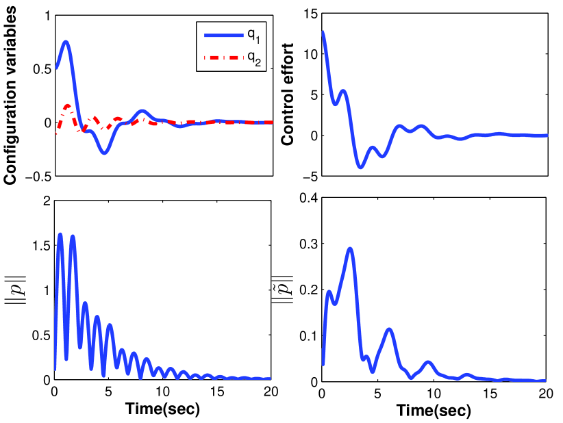
IV-A Ball and Beam System

The system consists of a ball moving along a beam whose angle is controlled. The position of the ball with respect to the pivot point of the beam is denoted by $q_{1}$, and the angle of the beam with respect to the vertical line is given by $q_{2}$. The dynamic parameters of the system are chosen based on the model given in [7],

$$M=\begin{bmatrix}1&0\\ 0&L^{2}+q_{1}^{2}\end{bmatrix},\qquad\quad V=gq_{1}\sin(\theta),$$

where $L$ is the half length of the beam, $\theta$ is the beam angle, and $g$ is the gravity constant. For the control law we utilize the proposed controller in [7] with the desired parameters of the closed-loop system, given by:

$$M_{d} =\begin{bmatrix}\sqrt{2}(L^{2}+q_{1}^{2})^{1/2}&L^{2}+q_{1}^{2}\\ L^{2}+q_{1}^{2}&\sqrt{2}(L^{2}+q_{1}^{2})^{3/2}\end{bmatrix}$$

$$V_{d} =g[1-\cos(q_{2})]+\frac{k_{p}}{2}\big{[}q_{2}-\frac{1}{\sqrt{2}}\mbox{arcsinh}(\frac{q_{1}}{L})\big{]}^{2}$$

$$J_{2} =\begin{bmatrix}0&j\\ -j&0\end{bmatrix},\quad j=q_{1}[p_{1}-\sqrt{2}(L^{2}+q_{1}^{2})^{-1/2}p_{2}],$$

in which $L=2m$, $R=\mbox{diag}\{0.2,0.1\}$, and the gains of the controller are $k_{p}=5$ and $k_{v}=5$ based on [14]. The initial condition of the robot is considered to be $[q^{T}(0),p^{T}(0)]=$ $[0.5,-0.1,0.1,0]$ based on Proposition 5 of [7] and the controller is supposed to position the ball at the equilibrium point $[q^{T}(0),p^{T}(0)]=$ $[0,0,0,0]$. With the given parameters, $H_{d}(0)=0.24$ is less than $0.31$ derived from Proposition 5 of [7], which ensures that the ball is always on the beam. Note that we do not modify the homogeneous solution of $V_{d}$ to utilize the analysis proposed in [7]. The parameters in Theorem 1 are derived after some cumbersome calculation as follows:

$$c_{V_{2}}=10.4,\qquad\quad c_{V_{d}}=2.4,\qquad\quad c_{\gamma_{2}}=6,$$

$$c_{M_{2}}=0,\hskip 5.69054pt\quad\qquad c_{M_{d}}=0.9,\qquad\quad c_{J}=10.4,$$

$$\lambda_{M}\{M_{d}^{-1}\}=0.82,\qquad\quad\hskip 2.84526pt\lambda_{m}\{M_{d}^{-1}\}=0.06$$

Using (12) one can simply compute $c_{p}=2$ and $c_{\tilde{p}}=0.44$, thus the upper bound of the control input will be $20$. The simulation results are depicted in Fig. 1. The control effort is less than 15 which is clearly less that than the upper bound obtained from (14). The upper bound of $\|p\|$ and $\|\tilde{p}\|$ are about 1.6 and 0.3 which are less than $c_{P}$ and $c_{\tilde{p}}$, respectively. Notice that the reason of difference between the actual and the computed upper bound is that in (14) we consider the worst-case scenario in obtaining the upper bounds.

Figure 1: Simulation results of the ball and beam system.

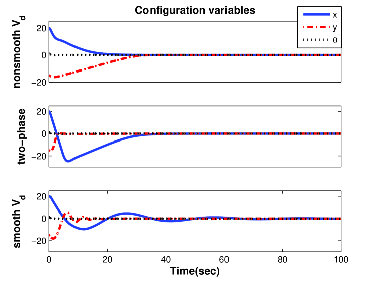
IV-B VTOL Aircraft

In the previous example, the effects of velocity-dependent terms was investigated. Through this example we aim to analyze the Remarks 2, 3 and 4. Hence, we consider an UMS with strongly coupled dynamics, referred to as VTOL. First a non-smooth control law is derived and the tracking performance of the system and the magnitude of the control effort is analysed. Secondly we propose a two-phase controller to compensate for the effects of non-smooth control law. Finally for the comparison purpose the performance of a smooth control law is also investigated. The dynamic model of the VTOL is given in [16] as follow:

$$M=I,\quad V=gy,\quad q=\begin{bmatrix}x\\ y\\ \theta\end{bmatrix},\quad G(q)=\begin{bmatrix}-\sin(\theta)&\epsilon\cos(\theta)\\ \cos(\theta)&\epsilon\sin(\theta)\\ 0&1\end{bmatrix}$$

where $x,y$ is the position of the center of gravity, $\theta$ is the roll angle and $\epsilon$ denotes the effect of the slopped wings. The purpose is to stabilize the unstable equilibrium point $[x^{*},y^{*},0]$ with bounded input IDA-PBC controller. In [16] an IDA-PBC controller with state-dependent $M_{d}$ and smooth $V_{d}$ is designed. Here, in order to analyze the effects of non-smooth terms, intentionally a locally stabilizing controller with constant $M_{d}$ and non-smooth $\nabla_{q}V_{d}$ is applied. The parameters of the controller are chosen as:

$$M_{d} =\begin{bmatrix}20\epsilon^{2}&0&\epsilon\\ 0&1&0\\ \epsilon&0&0.1\end{bmatrix},\qquad J_{2}=0_{3\times 3},$$

$$V_{d} =k_{1}\ln\cosh\Big{(}\epsilon(y-y^{*})+\ln\big{(}\epsilon\cos(\theta)-0.1\epsilon\big{)}\Big{)}$$

$$+k_{2}\ln\cosh\Big{(}\frac{1}{20\epsilon}(x-x^{*})-\theta-0.1\text{arctanh}\big{(}1.1055\tan(\frac{\theta}{2})\big{)}\Big{)}$$

$$-k_{1}\epsilon\tanh\ln(0.9\epsilon)(y-y^{*})$$

$$-\frac{g+k_{1}\epsilon\tanh\ln(0.9\epsilon)}{\epsilon}\ln\big{(}\epsilon\cos(\theta)-0.1\epsilon\big{)}-\rho,$$

with $k_{1},k_{2}\in\mathbb{R}^{+}$ being the free parameters and the constant $\rho$ is determined such that $V_{d}(t_{0})=0$. It is clear that the terms $\text{arctanh}\big{(}1.1055\tan(\frac{\theta}{2})\big{)}$ and $\ln\big{(}\epsilon\cos(\theta)-0.1\epsilon\big{)}$ confine $\theta$ in a region inside the workspace and lead to non-smooth terms in $\nabla_{q}V_{d}$. Hence, we invoke the results of Remark 3 and 4. Note that due to simple structure of $G$, it is possible to derive better upper bounds with respect to the conservative upper bound proposed in (20) by the following matrices,

$$(G^{T}G)^{-1}G^{T} =\begin{bmatrix}-\sin(\theta)&\cos(\theta)&0\\ \frac{\epsilon\cos(\theta)}{1+\epsilon}&\frac{\epsilon\sin(\theta)}{1+\epsilon}&\frac{1}{1+\epsilon}\end{bmatrix}$$

$$(G^{T}G)^{-1}G^{T}M_{d}M^{-1} =\begin{bmatrix}-20\epsilon^{2}\sin(\theta)&\cos(\theta)&-\epsilon\sin(\theta)\\ \frac{20\epsilon^{3}\cos(\theta)+\epsilon}{1+\epsilon}&\frac{\epsilon\sin(\theta)}{1+\epsilon}&\frac{\epsilon^{2}\cos(\theta)+0.1}{1+\epsilon}\end{bmatrix}$$

Figure 2: Configuration variables of the VTOL aircraft.

Figure 3: Control efforts of the VTOL aircraft.

In other words, a constant gravity is applied to the $y$ direction of the system. Thus, the bounds of controller are in the following form:

$$|\tau_{1}-g| \leq\max_{q}\{|g-\big{(}(G^{T}G)^{-1}G^{T}\nabla V\big{)}_{1}|\}$$

$$+\max_{q}\{\|(G^{T}G)^{-1}G^{T}M_{d}M^{-1}\|\}c_{V_{d}}+\lambda_{M}\{K_{v}\},$$

$$|\tau_{2}| \leq\max_{q}\{|\big{(}(G^{T}G)^{-1}G^{T}\nabla V\big{)}_{2}|\}$$

$$+\max_{q}\{\|(G^{T}G)^{-1}G^{T}M_{d}M^{-1}\|\}c_{V_{d}}+\lambda_{M}\{K_{v}\},$$ (22)

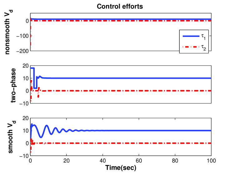
where the damping term is modified to be $K_{v}\mathcal{S}(G^{T}\tilde{p})$ with $\mathcal{S}$ defined in (8). The initial condition of the system is $[20,-15,1.3]^{T}$ and the desired position is the equilibrium point of the system at $[0,0,0]^{T}$. Since the initial value of $\theta$ is close to singularity, it results into high values for the control effort. Invoking Remark 3 one can compute the upper bound of $\theta=1.33$ by considering $k_{1}=4$ and $k_{2}=5$. By this means, the following upper bounds are derived after some calculations,

$$|\big{(}(G^{T}G)^{-1}G^{T}\nabla V\big{)}_{1}|\leq 10,\quad|\big{(}(G^{T}G)^{-1}G^{T}\nabla V\big{)}_{2}|\leq 2.25,$$

$$\|(G^{T}G)^{-1}G^{T}M_{d}M^{-1}\|\leq 1.75,\quad c_{V_{d}}=170$$

Simulation results with $K_{v}=I_{2}$ and $\mathcal{S}=\tanh$ is depicted in Fig. 2 and Fig. 3, denoted by ‘nonsmooth $V_{d}$’ in both figures. The simulation results of the two-phase controller and the smooth control law are also demonstrated in figures identified with the label ‘two-phase’ and ‘smooth $V_{d}$’, respectively. In Fig. 2 the tracking performance of the controller is shown, and Fig. 3 shows the control effort. As it is clear from the figures, for the non-smooth control law, the configuration variables converge to zero but the upper bound of the control effort is about 200 which is not even close to being applicable. To rectify this problem, a two-phase controller based on Remark 4 is designed. Additionally, the controller proposed in [16] is simulated. In the two-phase controller, the primary controller is used in the first phase to converge $\theta$ to zero. Hence, for a small value of the $\theta$, the dynamic of the system can be represented in the following form:

$$\ddot{x}\approx 0,\qquad\qquad\ddot{y}\approx\tau_{1}-g,$$

which is obtained by replacing $\theta\approx 0,\tau_{2}\approx 0$ in the dynamic of the system. Considering the simplified dynamic, then a secondary controller is designed using IDA-PBC approach such that $y-y^{*}$ converges to zero. Although with this controller $|x|$ will increase with a constant speed, it is possible to reduce $H_{d}(t_{0})$ arbitrary by increasing $M_{d_{(1,1)}}$ or decreasing $k_{2}$ in which $t_{0}$ denotes the initial time of applying the secondary controller. In the two-phase controller the primary controller is given by:

$$\tau_{1} =g-\varkappa_{1}\mathcal{S}(\kappa_{1}y+\kappa_{2}\dot{y})$$

$$\tau_{2} =-\varkappa_{2}\mathcal{S}(\kappa_{3}\theta+\kappa_{4}\dot{\theta})$$

with the following parameters:

$$\varkappa_{1}=\varkappa_{2}=8,\hskip 5.69054pt\kappa_{1}=30,\hskip 5.69054pt\kappa_{2}=20,\hskip 5.69054pt\kappa_{3}=80,\hskip 5.69054pt\kappa_{4}=30,$$

with this aim that $|\tau_{1}-g|\leq 10$ and $|\tau_{2}|<10$. Referring to the simulation results in Fig. 2 and Fig. 3, it is clear that after applying the IDA-PBC, the control efforts are in a the bounds, and configuration variables converge to their desired values. This shows the superiority of this method. Note that one may design a better controller for the first phase to prevent the increase of $|x|$, but this is out of the scope of this paper. We have also investigated the controller proposed in [16] which is based on a smooth $V_{d}$. The parameters of the controller are $P=\mbox{diag}\{0.003,0.005\}$ and $K_{v}=0.2I_{2}$ . The simulation results shows that $|\tau_{1}-g|$ and $|\tau_{2}|$ lies in the predefined range. It should be noted that, in this case we have considered smaller gains for the controller to have smaller control effort, in the expense of slow convergence rate. This study confirms that the suitable solution for the PDEs is an essential part of the controller design while considering bounded input control problems.

V Conclusion

In this paper we addressed the bounded input control of mechanical systems based on IDA-PBC approach. In IDA-PBC, the control law is formulated in terms of the the desired potential and kinetic energy for the closed-loop system, and we found the upper bound of each component. The desired potential and kinetic energy of the IDA-PBC are the solution of PDE and the upper bound of the potential energy are found by suitably defining the homogeneous solution of desired potential energy. For the upper bounds of the kinetic energy related term, the velocity related terms are complex to deal with and we proposed a method to find the upper bounds of the velocity. It is also discussed that how the gains of the controller and the solution of the PDEs are to be chosen and how the selection of the design parameters affects the performance of the closed-loop system. The bounded input control of IDA-PBC control is investigated for potential energy shaping as well as constant mass matrix systems in literature, and the proposed method includes kinetic energy shaping for configuration dependant mass matrix. The proposed method is also extended for systems with non-symmetric control bounds as well as for the systems with state-dependent input coupling matrix. Moreover, we proposed a methodology to deal with non-smooth control inputs with a two-phase control scheme. The validity and the application of the proposed method is further investigated through simulation studies for two benchmark underactuated mechanical systems.

References

- [1] B. He, S. Wang, and Y. Liu, “Underactuated robotics: a review,” International Journal of Advanced Robotic Systems, vol. 16, no. 4, p. 1729881419862164, 2019.
- [2] R. Xu and Ü. Özgüner, “Sliding mode control of a class of underactuated systems,” Automatica, vol. 44, no. 1, pp. 233–241, 2008.
- [3] R. Ortega and M. W. Spong, “Adaptive motion control of rigid robots: A tutorial,” Automatica, vol. 25, no. 6, pp. 877–888, 1989.
- [4] R. Ortega, A. Van Der Schaft, B. Maschke, and G. Escobar, “Interconnection and damping assignment passivity-based control of port-controlled hamiltonian systems,” Automatica, vol. 38, no. 4, pp. 585–596, 2002.
- [5] M. Takegaki and S. Arimoto, “A new feedback method for dynamic control of manipulators,” Journal of Dynamic Systems, Measurement, and Control, vol. 103, no. 2, pp. 119–125, 1981.
- [6] R. Ortega, I. Mareels, A. van der Schaft, and B. Maschke, “Energy shaping revisited,” in Proceedings of the 2000. IEEE International Conference on Control Applications. Conference Proceedings (Cat. No. 00CH37162). IEEE, 2000, pp. 121–126.
- [7] R. Ortega, M. W. Spong, F. Gómez-Estern, and G. Blankenstein, “Stabilization of a class of underactuated mechanical systems via interconnection and damping assignment,” IEEE transactions on automatic control, vol. 47, no. 8, pp. 1218–1233, 2002.
- [8] P. Borja, R. Cisneros, and R. Ortega, “Shaping the energy of port-hamiltonian systems without solving pde’s,” in 2015 54th IEEE Conference on Decision and Control (CDC). IEEE, 2015, pp. 5713–5718.
- [9] M. R. J. Harandi and H. D. Taghirad, “On the matching equations of kinetic energy shaping in ida-pbc,” arXiv preprint arXiv:2011.14958, 2020.
- [10] J. G. Romero, R. Ortega, and A. Donaire, “Energy shaping of mechanical systems via pid control and extension to constant speed tracking,” IEEE Transactions on Automatic Control, vol. 61, no. 11, pp. 3551–3556, 2016.
- [11] E. Zergeroglu, W. Dixon, A. Behal, and D. Dawson, “Adaptive set–point control of robotic manipulators with amplitude–limited control inputs,” Robotica, vol. 18, no. 2, pp. 171–181, 2000.
- [12] M. Spong, J. Thorp, and J. Kleinwaks, “The control of robot manipulators with bounded input,” IEEE Transactions on Automatic Control, vol. 31, no. 6, pp. 483–490, 1986.
- [13] V. Santibanez, R. Kelly, and J. Sandoval, “Control of the inertia wheel pendulum by bounded torques,” in Proceedings of the 44th IEEE Conference on Decision and Control. IEEE, 2005, pp. 8266–8270.
- [14] F. Gómez-Estern and A. J. Van der Schaft, “Physical damping in ida-pbc controlled underactuated mechanical systems,” European Journal of Control, vol. 10, no. 5, pp. 451–468, 2004.
- [15] A. Donaire, R. Ortega, and J. G. Romero, “Simultaneous interconnection and damping assignment passivity-based control of mechanical systems using dissipative forces,” Systems & Control Letters, vol. 94, pp. 118–126, 2016.
- [16] J. A. Acosta, R. Ortega, A. Astolfi, and A. D. Mahindrakar, “Interconnection and damping assignment passivity-based control of mechanical systems with underactuation degree one,” IEEE Transactions on Automatic Control, vol. 50, no. 12, pp. 1936–1955, 2005.
- [17] I. N. Sneddon, Elements of partial differential equations. Courier Corporation, 2006.
- [18] A. Loria, R. Kelly, R. Ortega, and V. Santibanez, “On global output feedback regulation of euler-lagrange systems with bounded inputs,” IEEE Transactions on Automatic Control, vol. 42, no. 8, pp. 1138–1143, 1997.
- [19] H. K. Khalil and J. Grizzle, Nonlinear systems. Prentice hall Upper Saddle River, NJ, 2002, vol. 3.
- [20] M. R. J. Harandi and H. D. Taghirad, “Motion control of an underactuated parallel robot with first order nonholonomic constraint,” in 2017 5th RSI International Conference on Robotics and Mechatronics (ICRoM). IEEE, 2017, pp. 582–587.
- [21] M. Harandi, S. Khalilpour, H. Damirchi, and H. D. Taghirad, “Stabilization of cable driven robots using interconnection matrix: Ensuring positive tension,” in 2019 7th International Conference on Robotics and Mechatronics (ICRoM). IEEE, 2019, pp. 235–240.
- [22] R. W. Brockett et al., “Asymptotic stability and feedback stabilization,” Differential geometric control theory, vol. 27, no. 1, pp. 181–191, 1983.
- [23] M. W. Spong, “Energy based control of a class of underactuated mechanical systems,” IFAC Proceedings Volumes, vol. 29, no. 1, pp. 2828–2832, 1996.
- [24] A. Zavala-Rio and V. Santibanez, “A natural saturating extension of the pd-with-desired-gravity-compensation control law for robot manipulators with bounded inputs,” IEEE Transactions on Robotics, vol. 23, no. 2, pp. 386–391, 2007.
- [25] R. Ortega, J. A. L. Perez, P. J. Nicklasson, and H. J. Sira-Ramirez, Passivity-based control of Euler-Lagrange systems: mechanical, electrical and electromechanical applications. Springer Science & Business Media, 2013.