The Golden Ratio and Hydrodynamics

Abstract

There are useful and useless golden ratios. The useful one helps in traffic. The useless and rather mysterious one arises in hydrodynamics of point vortices, which we discuss in detail.

He [Radishchev] wanted simultaneously to write a subtle, graceful, and witty prose, but also to serve his fatherland… For mixing the genres Radishchev got jailed for ten years.

Pyotr Vail and Alexander Genis, Native Speech

Mysterious Golden Ratios

There are useful and useless golden ratios. We start with the former.

The best way to convert miles to kilometers is to take the next Fibonacci number. Indeed, 5 mi is 8 km, or 55 mi/h (the most important speed limit in the USA until 1995) is 89 km/h. Conversely, take the previous Fibonacci number: 34 km is 21 mi, or 130 km/h (the speed limit in France) corresponds to 80 mi/h (one can always squeeze in extra zeros to the Fibonacci pair 13 and 8); see Figure 2.

A justification for this simple rule is that in the Fibonacci sequence

$$1,1,2,3,5,8,13,21,34,55,89,144,\dots$$

the ratio of two consecutive terms tends to the golden ratio (or golden section)

$$\phi=\frac{\sqrt{5}+1}{2}=1.618034...$$

as we go along the sequence. The latter differs from the mile/kilometer factor $mi/km=1.6093$ by about $0.5\%$ (which is better than the precision of the police radar detector), hence the above mnemonic rule.

There are many equivalent definitions of the golden ratio. The basic one is that this is the ratio of length to width for a rectangle, which preserves this ratio after cutting out the square; see Figure 2. Symbolically, $\phi:=a/b=b/(a-b)$, which implies that $\phi$ is the positive root of the quadratic equation $\phi^{2}-\phi-1=0$.

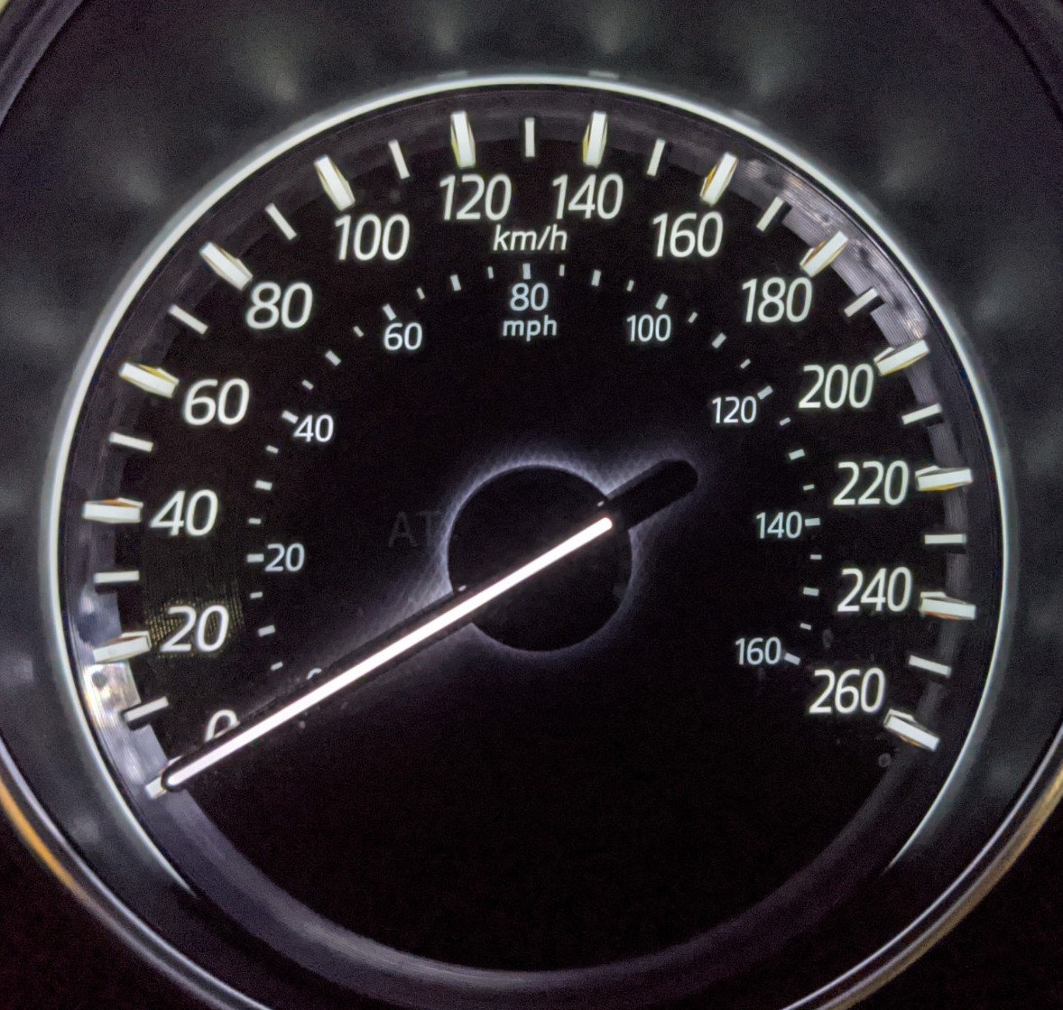
Figure 1: The Mazda CX-5 speedometer with both $km/h$ and $mph$ scales.

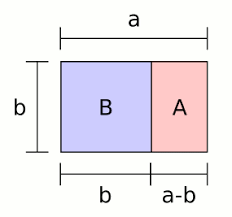
Figure 2: The golden ratio $\phi=a/b$ is the ratio of length to width for such a special rectangle.

There are plenty of appearances and applications of the golden ratio in the medieval architecture, phyllotaxis, mollusk shells, one-dimensional dynamics, etc. Here we describe the recently discovered, rather mysterious, and, likely, most useless appearance of the golden ratio in 2D hydrodynamics.

Dynamics of point vortices

The evolution of the earth atmosphere or oceans is often thought of as a motion of an inviscid incompressible two-dimensional fluid. The classical Euler equation for such a motion can be written in the vorticity form $\partial_{t}\omega+L_{v}\omega=0$, describing that the fluid’s vorticity $\omega:={\rm curl}\,v$ is transported by the fluid flow with velocity $v$. In two dimensions the vorticity $\omega$ is a function, and the Euler equation assumes the form

$$\partial_{t}\omega=\frac{\partial\psi}{\partial x}\frac{\partial\omega}{\partial y}-\frac{\partial\psi}{\partial y}\frac{\partial\omega}{\partial x}\,,$$

where the stream function $\psi$ of the flow satisfies $\Delta\psi=\omega$.

This infinite-dimensional system in turn can be viewed as a limit of dynamics of so-called point (or singular) vortices. A description of the corresponding finite-dimensional dynamical system of vortices in the plane goes back to Helmholtz and Kirchhoff; see e.g. [6, 7, 3]. Namely, let the vorticity $\omega$ be supported on $N$ point vortices $\omega=\sum^{N}_{j=1}\Gamma_{j}\,\delta(z-z_{j})$, where $z_{j}=(x_{j},y_{j})$ are coordinates and $\Gamma_{j}$ is the strength of the $j$th point vortex in the plane $\mathbb{R}^{2}=\mathbb{C}$. Then the evolution of $N$ vortices according to the Euler equation is described by the system

$$\Gamma_{j}\dot{x}_{j}=\frac{\partial\mathcal{H}}{\partial y_{j}},\qquad\Gamma_{j}\dot{y}_{j}=-\frac{\partial\mathcal{H}}{\partial x_{j}},\qquad 1\leq j\leq N\,,$$

for the function

$$\mathcal{H}(z_{1},...,z_{N})=-\frac{1}{4\pi}\sum^{N}_{j<k}\Gamma_{j}\Gamma_{k}\,\ln|z_{j}-z_{k}|$$

on $(\mathbb{R}^{2})^{N}$. This system first appeared in this modern form in the 1876 Berlin lectures [7] by Gustav Kirchhoff (1824-1887), who also found the system’s three first integrals, related to its invariance with respect to the three-dimensional group $E(2)$ of motions of the plane.

Remark 1.

The function $\mathcal{H}$ is the system’s Hamiltonian for the standard Poisson bracket on $\mathbb{R}^{2N}$ weighted by the strengths $\Gamma_{j}$. In addition to the Hamiltonian function, there are two first integrals in involution that are coming from Noether’s symmetries. This implies the integrability for small number of vortices: it turns out that the systems of $N=1,2$ and 3 point vortices in the plane $\mathbb{R}^{2}$ are completely integrable, while the systems of $N\geq 4$ point vortices for generic strengths are not; see e.g. [3].

The cases of one and two point vortices were already studied in detail by Hermann von Helmholtz (1821-1894) some twenty years earlier, in his 1858 paper [6]. He discovered that a single point vortex ($N=1$) in the plane stays at rest, while a pair of point vortices ($N=2$) rotates about their common center of vorticity $z_{c}:=(\Gamma_{1}z_{1}+\Gamma_{2}z_{2})/(\Gamma_{1}+\Gamma_{2})$. For instance, the vortex pair with $\Gamma_{1}=\Gamma_{2}$ rotates about its midpoint, Figure 3a. For generic $\Gamma_{1},\Gamma_{2}$ the rotation center is located on the line joining the vortices, and it is between the vortices provided that their strengths are of the same sign, and outside the segment joining them if they are of different signs. In the case where the vortices form a dipole, i.e., a pair with $\Gamma_{1}=-\Gamma_{2}$, they move uniformly along its perpendicular bisector, Figure 3b, and this can be regarded as a rotation about a center at infinity. (The case of two point vortices is of particular interest in meteorology; see [4]. For instance, the dipole setting corresponds to the cyclone–anticyclone pair moving in the zonal direction; see Figure 4.)

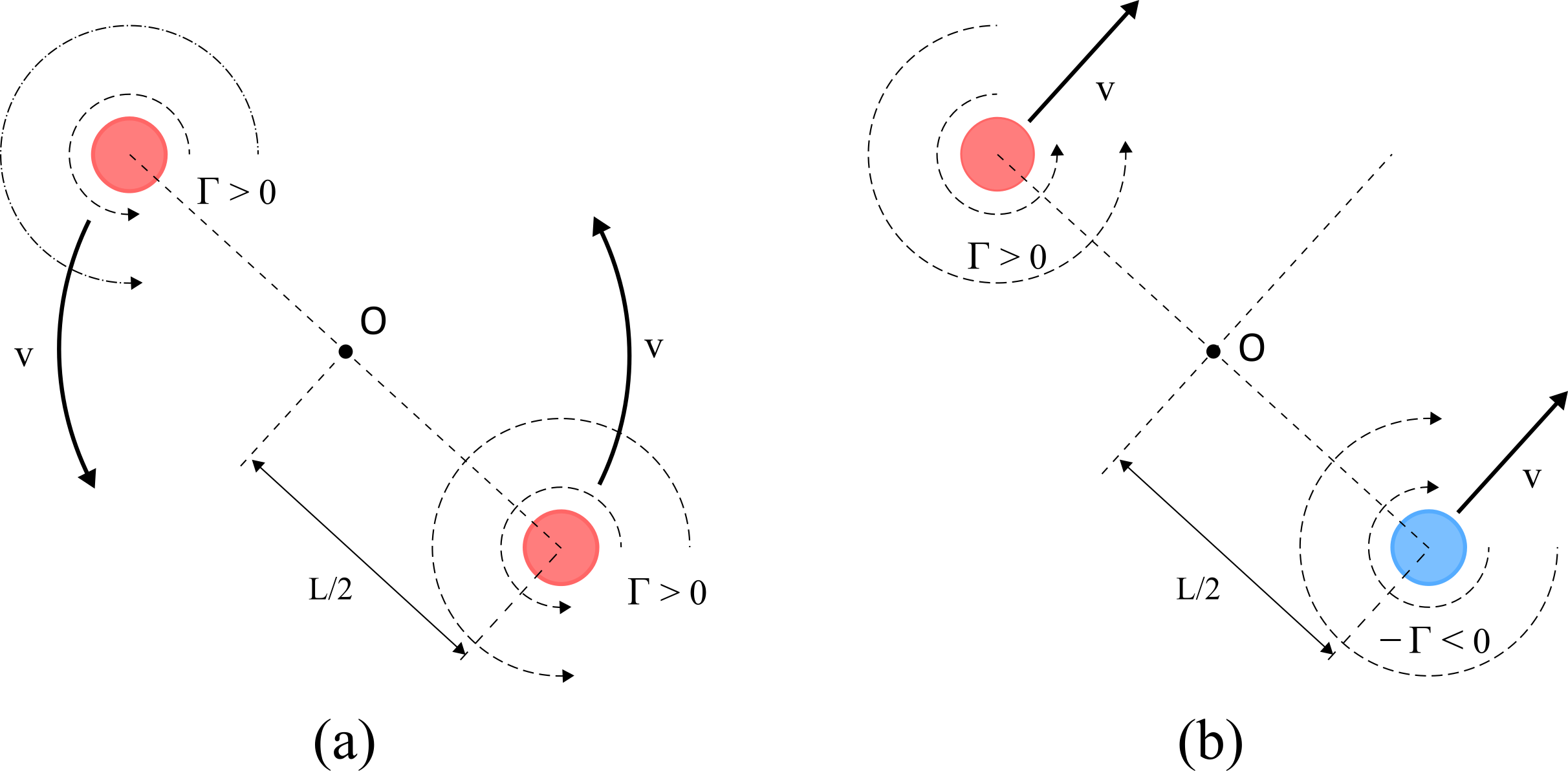
Figure 3: Systems of two vortices: a) a pair of point vortices of equal strengths rotates about their center, b) a dipole moves with constant velocity along its perpendicular bisector.

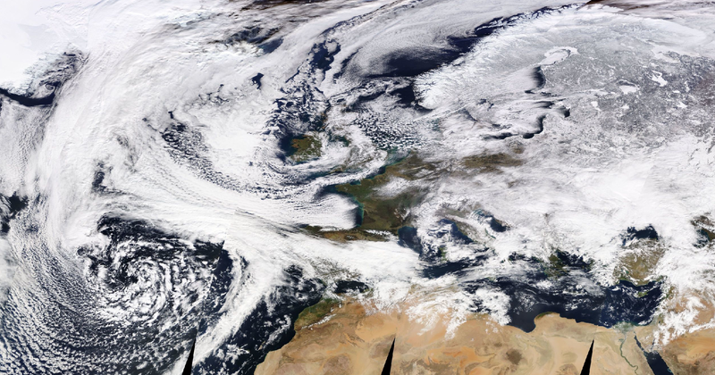
Figure 4: The interaction of Cyclone Emma (nearing from the SW) and Anticyclone Hartmut (covering Europe from the NE) on February 27, 2018 (NASA, Wiki-Commons).

The motion of three point vortices ($N=3$) is still integrable but can be much more elaborate, and it was described in detail by Walter Gröbli in his dissertation in 1877 [5]. Gröbli was a student of Heinrich Weber and took courses of Kirchhoff, Helmholtz, Kummer, and Weierstrass in Berlin; see more details to this story in [2]. In particular, he discovered that unlike the two-vortex case, three vortices allow self-similar collapsing solutions; see Figure 5. (Note that point vortices can never have pairwise collisions, even in many-vortex motions, since when only two point vortices approach each other, their interaction with other vortices is weakening, and they start behaving like a two-vortex system, therefore approximately rotating around their common vorticity center.)

It is worth mentioning that unlike the famous three-body problem, which requires specifying both positions and velocities as its initial conditions, the three-vortex problem requires only vortex positions to determine the resulting trajectory.

Figure 5: Self-similar motion in which the vortex triangle changes its size but not its shape (a drawing from W. Gröbli’s 1877 dissertation). This self-similar expansion corresponds to vortices of strengths $\Gamma_{1}=3,\Gamma_{2}=-2$ and $\Gamma_{3}=6$; see [2].

Remark 2.

It is interesting to trace how the motion of vortices changes on domains with boundary. Already the half-plane brings a wider variety to this classical problem. Indeed, the motion of point vortices in a half-plane can be obtained by considering the auxiliary reflected point vortices, so that the Green function for the Laplacian $\Delta\psi=\omega$ on the half-plane satisfies the zero boundary condition. An interesting feature of this motion is that, while a single vortex in the whole plane does not move, a single vortex is the half-plane moves parallel to the boundary with constant speed, in a sense “interacting with the boundary”. Indeed, its motion is equivalent to the motion of a dipole in $\mathbb{R}^{2}$ with auxiliary point vortex of opposite strength reflected in the boundary, while the boundary becomes the perpendicular bisector for such a pair.

For two point vortices in the half-plane one observes many types of motions, some of which are of particular interest. For instance, it allows a leapfroging motion along the border, which is also related to the famous leapfrogging motion of axisymmetric vortex rings in 3D. We detail the motion of two point vortices in a half-plane in the next section.

It is worth pointing out that the system in the half-plane is invariant only under translations parallel to the boundary, and hence has only one Noether invariant. Thus this Hamiltonian system of point vortices in the half-plane is integrable for $N=1$ and 2, while for $N=3$ it was recently proven to be non-integrable [8].

A pair of point vortices in the half-plane

Here we will study the motion of two point vortices in the half-plane for two special but representative cases: a vortex pair or a dipole, which are two point vortices of the same absolute strengths and having, respectively, either the same or the opposite signs.

For two point vortices of any strengths $\Gamma_{1}$ and $\Gamma_{2}$ located at $z_{1}=(x_{1},y_{1})$ and $z_{2}=(x_{2},y_{2})$ in the half-plane the corresponding Hamiltonian takes into account their interaction between themselves and with their mirror images $\bar{z}_{1}=(x_{1},-y_{1})$ and $\bar{z}_{2}=(x_{2},-y_{2})$ of strengths $-\Gamma_{1}$ and $-\Gamma_{2}$:

$$\mathcal{H}(z_{1},z_{2})=\frac{1}{4\pi}\left(\Gamma_{1}^{2}\log|z_{1}-\bar{z}_{1}|+\Gamma_{2}^{2}\log|z_{2}-\bar{z}_{2}|-2\Gamma_{1}\Gamma_{2}\log|z_{1}-z_{2}|+2\Gamma_{1}\Gamma_{2}\log|z_{1}-\bar{z}_{2}|\right)\,.$$

The Noether first integral is $P:=\Gamma_{1}y_{1}+\Gamma_{2}y_{2}$, which corresponds to the system symmetry with respect to the $x$-translations.

To study vortex bifurcations we normalize their strengths by setting $\Gamma_{1}=\Gamma_{2}=1$ for a vortex pair and $\Gamma_{1}=-\Gamma_{2}=1$ for a dipole. Furthermore, introduce the following dimensionless parameter $W:=P^{2}\exp(-4\pi\mathcal{H})$ measuring the vortex interaction. As we will see below, the increase of $W$ corresponds to the weakening of the interaction between the point vortices.

Remark 3.

To see that this is indeed a dimensionless parameter, one observes that whatever units of length are used for $x$ and $y$, the value of $P^{2}$ is measured in $units^{2}$, while $\exp(-\mathcal{H})$ is measured in $units^{-2}$, so that $W$ is dimensionless. More generally, before normalizations, one can define dimensionless $W:=(P/\Gamma)^{2}\exp(-4\pi\mathcal{H}/\Gamma^{2})$, where $\Gamma:=\Gamma_{1}=\pm\Gamma_{2}$.

By changing this parameter one observes different types of behaviour for the corresponding vortex systems. As $W$ increases, the interaction of vortices weakens: in a dipole, upon approaching one another the vortices either go to infinity at a slanted asymptote, or one of them makes a kink with the other before parting, or they pass each other at a social distance; see Figure 6.

Figure 6: As the interaction weakens, the vortices in the dipole either go to infinity, or one of them makes a kink, or they pass around each other. (The orange and aquamarine colors correspond to two vortices 1 and 2).

For a vortex pair, a strong interaction is related to a leap-frogging motion of the vortices, while a weak one produces just two intertwining sinusoidal-like trajectories; see Figure 7. In both cases the change from a kink/leap-frogging motion to a regular one happens through the cusp-type bifurcation for the vortex motion:

Figure 7: For a vortex pair, as the interaction weakens, a leap-frogging motion of the vortices changes to intertwining sinusoidal-like trajectories via a cusp-type motion.

Theorem 4.

(i) For a vortex pair the leap-frogging vortex motion changes to the smooth intertwining one through the cusp bifurcation, which occurs at the reciprocal golden ratio value of its interaction parameter: $W=1/\phi$.

(ii) For a dipole the bifurcation from the kink motion to the laminar one occurs through the cusp bifurcation, corresponding to the golden ratio value of its interaction parameter: $W=\phi$.

(iii) At the moment of cusp bifurcation the two vortices lie on the same vertical. The cross-ratio of the four points $(z_{1},z_{2},\bar{z}_{2},\bar{z}_{1})$, that are these two vortices together with their mirror images, is equal to the golden ratio $\phi$ (in both cases, for a vortex pair and a dipole).

Before we prove this theorem we make several observations for general strengths $\Gamma_{1}$ and $\Gamma_{2}$ of two vortices in the half-plane. First of all, note that the cusp in a generic parametrized curve $t\mapsto(x(t),y(t))$ in the plane corresponds to the vanishing derivative, $(\dot{x}(t),\dot{y}(t))=(0,0)$, an instantaneous stop. (Indeed, a generic curve $(x(t),y(t))=(a_{0}+a_{2}t^{2}+a_{3}t^{3}+...,b_{0}+b_{2}t^{2}+b_{3}t^{3}+...)$ with vanishing derivative at $t=0$ can be transformed by local coordinate changes to $(x(t),y(t))=(t^{3},t^{2})$, a normal form of a cusp.)

Let us rewrite the general two-vortex Hamiltonian in a more explicit coordinate form:

$$\mathcal{H}(z_{1},z_{2})=\frac{1}{4\pi}\log\left((2y_{1})^{\Gamma_{1}^{2}}(2y_{2})^{\Gamma_{2}^{2}}\left(\frac{(x_{1}-x_{2})^{2}+(y_{1}+y_{2})^{2}}{(x_{1}-x_{2})^{2}+(y_{1}-y_{2})^{2}}\right)^{\Gamma_{1}\Gamma_{2}}\right)\,.$$

Recall one useful property of such a system: it does not allow collisions of vortices between themselves and with the boundary [8]. We start with the following auxiliary statement.

Lemma 5.

For a pair of vortices in the half plane, the velocity of either of the vortices is horizontal whenever the two vortices turn out to be on the same vertical, $x_{1}=x_{2}$.

Proof.

For instance for vortex $z_{1}$ we obtain:

$$\dot{y}_{1}=-\frac{1}{\Gamma_{1}}\frac{\partial\mathcal{H}}{\partial x_{1}}=-\frac{\Gamma_{2}}{4\pi}\left(\frac{2(x_{1}-x_{2})}{(x_{1}-x_{2})^{2}+(y_{1}+y_{2})^{2}}-\frac{2(x_{1}-x_{2})}{(x_{1}-x_{2})^{2}+(y_{1}-y_{2})^{2}}\right)$$

$$=\frac{2\Gamma_{2}}{\pi}\frac{(x_{1}-x_{2})y_{1}y_{2}}{\left((x_{1}-x_{2})^{2}+(y_{1}+y_{2})^{2}\right)\left((x_{1}-x_{2})^{2}+(y_{1}-y_{2})^{2}\right)}\,.$$

Since the vortices in the half-plane never hit the boundary, one has $y_{1}y_{2}\not=0$, which implies that the velocity of $z_{1}=(x_{1},y_{1})$ is horizontal, i.e., $\dot{y}_{1}=0$ iff $x_{1}-x_{2}=0$. ∎

Note at the moment when the line connecting the two vortices becomes vertical it passes through their mirror images as well.

Lemma 6.

At the moment of instantaneous stop, the heights of the vortices are related by a factor of $2\lambda+\sqrt{4\lambda^{2}+1}$, i.e., $y_{1}=(2\lambda+\sqrt{4\lambda^{2}+1})y_{2}$, where $\lambda:=\Gamma_{2}/\Gamma_{1}$.

Proof.

Indeed, for the vortex $z_{1}$ we have:

$$\dot{x}_{1}=\frac{1}{\Gamma_{1}}\frac{\partial\mathcal{H}}{\partial y_{1}}=\frac{\Gamma_{1}}{4\pi y_{1}}+\frac{\Gamma_{2}}{4\pi}\left(\frac{2(y_{1}+y_{2})}{(x_{1}-x_{2})^{2}+(y_{1}+y_{2})^{2}}-\frac{2(y_{1}-y_{2})}{(x_{1}-x_{2})^{2}+(y_{1}-y_{2})^{2}}\right)\,.$$

Upon plugging in the condition $x_{1}-x_{2}=0$, which ensures $\dot{y}_{1}=0$, we obtain

$$\dot{x}_{1}=\frac{\Gamma_{1}}{4\pi y_{1}}-\frac{\Gamma_{2}y_{2}}{\pi(y_{1}^{2}-y_{2}^{2})}=\frac{1}{4\pi}\frac{\Gamma_{1}y_{1}^{2}-\Gamma_{1}y_{2}^{2}-4\Gamma_{2}y_{1}y_{2}}{y_{1}(y_{1}^{2}-y_{2}^{2})}\,.$$

The denominator can never be zero, due to the absence of collisions between vortices and with the boundary. Equating the numerator to zero and solving the corresponding equation $\Gamma_{1}y_{1}^{2}-\Gamma_{1}y_{2}^{2}-4\Gamma_{2}y_{1}y_{2}=0$ for a positive root, since both $y_{1}$ and $y_{2}$ are positive, we come to $y_{1}/y_{2}=2\lambda+\sqrt{4\lambda^{2}+1}$ with $\lambda:=\Gamma_{2}/\Gamma_{1}$. ∎

Now we will set $\Gamma_{1}=\pm\Gamma_{2}$ and prove the theorem for a dipole and a vortex pair.

Proof.

For a dipole $\lambda=-1$, and hence $y_{1}=(-2+\sqrt{5})y_{2}$ and $y_{1}^{2}-y_{2}^{2}+4y_{1}y_{2}=0$. Then

$$W=P^{2}\exp(-4\pi\mathcal{H})=\frac{(y_{1}-y_{2})^{2}(y_{1}+y_{2})^{2}}{4y_{1}y_{2}(y_{1}-y_{2})^{2}}=\frac{y_{1}+y_{2}}{y_{2}-y_{1}}=\frac{-1+\sqrt{5}}{3-\sqrt{5}}=\frac{1+\sqrt{5}}{2}=\phi\,.$$

The computation with $\lambda=1$ for a vortex pair is similar.

The cross-ratio of four points $(y_{1},y_{2},y_{3},y_{4})$ on a line is defined as

$${\rm CR}(y_{1},y_{2},y_{3},y_{4})=\frac{(y_{1}-y_{4})(y_{2}-y_{3})}{(y_{1}-y_{2})(y_{3}-y_{4})}\,.$$

One immediately obtains that, e.g., ${\rm CR}(2+\sqrt{5},\,1,-1,-2-\sqrt{5})=(1+\sqrt{5})/2=\phi$. ∎

Remark 7.

For a general strength ratio $\lambda:=\Gamma_{2}/\Gamma_{1}$ the dimensionless interaction parameter is $W(\lambda):=|P/\Gamma|^{1+\lambda^{2}}\exp(-4\pi\mathcal{H}/\Gamma^{2})$. By plugging in it the relation of instantaneous stop from the two lemmas above, one can obtain the whole bifurcation diagram of this system.

Returning to the case of $\lambda=\pm 1$ we recall that at the moment of instantaneous stop both point vortices, and hence their mirror images, lie on the same vertical. The cusp itself is related to the fact that at a specific value of $W$, controlling the interconnection, a dominant interaction between the vortices gets overridden by the interaction with their mirrors. This balanced proportion of distances between the vortices on the vertical line leads to the golden ratio due to the following more general observation.

Consider a point $E=1$ on the real axis and an action of three other points on it. We will be looking for a point $A>1$ satisfying the following condition: its “action” on the point $E$ combined with the action of its mirror point $-A$ on $E$ is balanced by the action of the mirror image $-E$ on $E$ itself.

Lemma 8.

Assume that the action is inverse proportional to the distance between the points. Then the cross-ratio of points $(A,E,-E,-A)$ satisfying the balance of actions is equal to the golden ratio:

$${\rm CR}(A,E,-E,-A)=\phi\,.$$

Proof.

The balance of actions reduces to the equation

$$\frac{1}{A-1}+\frac{1}{A+1}=\frac{1}{2}\,,$$

where $1/2$ arises as the reciprocal of the distance between $E=1$ and $-E=-1$. Then $A$ satisfies the quadratic equation $A^{2}-4A-1=0$, and therefore $A=2\pm\sqrt{5}$. By choosing the positive root we come to the same cross-ratio as in Theorem 4$(iii)$. ∎

For the system of point vortices this “action” is the speed that the vortices induce on one another, while their balance means the instantaneous stop. The induced speed is indeed inverse proportional to the distance: if the vorticity is $\omega=\delta(z)$ on ${\mathbb{C}}={\mathbb{R}}^{2}$, then the stream function is $\psi=\Delta^{-1}\omega=C\ln|z|$, and hence the fluid velocity $v$ has the property $|v|=|{\rm sgrad}\,\psi|\sim 1/|z|$ at the distance $|z|$ from the origin.

While this explains the cross-ratio part of the theorem, the appearance of the golden ratio in the interaction parameter in this hydrodynamical context of Helmholtz singular vortices remains elusive.

Acknowledgments. We are indebted to Klas Modin and Cheng Yang for helpful discussions. This work was partially supported by an NSERC research grant.

References

- [1]
- [2] H. Aref, N. Rott, and H. Thomann, Gröbli’s solution of the three-vortex problem. Annual Review of Fluid Mechanics, vol. 24 (1992), 1-21.
- [3] V. I. Arnold and B. A. Khesin, Topological methods in hydrodynamics. Springer, 1998, 374pp.
- [4] F.V. Dolzhansky, Fundamentals of geophysical hydrodynamics. Encyclopaedia of Math. Sci.: Mathematical Physics, vol.103, Springer-Verlag, 2013, 272pp.
- [5] W. Gröbli, Specielle Probleme über die Bewegung geradliniger paralleler Wirbelfäden. (1877), Zürich: Zürcher und Furrer. 86 pp., Also published in Vierteljahrsschrift der Naturforschenden Gesellschaft in Zürich 22: 37-81; 129-65.
- [6] H. Helmholtz, On integrals of the hydrodynamical equations which express vortex-motion. (1858), Transl. P.G. Tait, 1867, in Phil. Mag. (4) 33: 485-512;
- [7] G.R. Kirchhoff, Vorlesungen über Mathematische Physik, Mechanik. (1877), Lecture 20. Leipzig: Teubner.
- [8] C. Yang, Vortex motion of the Euler and Lake equations, preprint arXiv:2009.12004, (2020), to appear on J. of Nonlinear Sci., 19pp.