On the Benefits of Traffic “Reprofiling”
The Single Hop Case

Jiayi Song,  Jiaming Qiu,  Roch Guérin,  and Henry Sariowan J. Qiu and R. Guérin are with the Computer Science and Engineering department at Washington University in St. Louis, Saint Louis, MO 63130, USA, e-mail: {qiujiaming,guerin}@wustl.edu.J. Song was with the Computer Science and Engineering department at Washington University in St. Louis and is now with ByteDance, Mountain View, CA 94041, USA, e-mail: jiayisong@wustl.edu.H. Sariowan is with Google, Mountain View, CA 94043, USA, e-mail hsariowan@google.com.An early version of the paper was presented at the 33rd International Teletraffic Congress (ITC’33) in September 2021.The work was supported by NSF grant CNS 2006530 and a gift from Google.
Abstract

The need to guarantee hard delay bounds to traffic flows with deterministic traffic profiles, e.g., token buckets, arises in a number of network settings. Of interest are solutions that offer such guarantees while minimizing network bandwidth. The paper explores a basic building block towards realizing such solutions, namely, a single hop configuration. The main results are in the form of optimal solutions for meeting local deadlines under schedulers of varying complexity and therefore cost. The results demonstrate how judiciously modifying flows’ traffic profiles, i.e., reprofiling them, can help simple schedulers reduce the bandwidth they require, often performing nearly as well as more complex ones.


©2024 IEEE. Personal use of this material is permitted. Permission from IEEE must be obtained for all other uses, in any current or future media, including reprinting/republishing this material for advertising or promotional purposes, creating new collective works, for resale or redistribution to servers or lists, or reuse of any copyrighted component of this work in other works.

Index Terms:
Latency, bandwidth, optimization, token bucket, scheduling.

I Introduction

The provision of deterministic delay guarantees to traffic flows is emerging as an important requirement in increasingly diverse settings. They include automotive, avionics, and manufacturing applications, smart grids, and datacenters [1, 2, 3, 4, 5, 6, 7]. This is reflected in standards such as Time Sensitive Networking (TSN) and Deterministic Networking (DetNet) [8, 9, 10, 11] and in the Service Level Objectives/Agreements (SLOs/SLAs)[12] of many service provider networks that are increasingly including latency targets, motivated in part by the rapid growth of edge computing offerings [13].

In such settings, the traffic eligible for latency guarantees is commonly controlled using a traffic regulator [14] in the form of a token bucket $(r,b)$ that limits both the flow’s long-term rate, $r$, and burstiness, $b$. A flow’s token bucket parameters are typically determined using traces, and selected to ensure zero access delay [15]. The network’s goal is then to ensure that the latency guarantees of all such rate-controlled flows are met, preferably with as little bandwidth as possible.

This is the environment this paper assumes, with a focus on a basic building block, namely, delivering latency guarantees on a single link (hop) with the least amount of bandwidth. The answer obviously depends on the type of scheduler controlling access to the link, and the paper considers schedulers of different levels of complexity. Of greater interest is whether, what the paper terms reprofiling, can be beneficial. Reprofiling amounts to modifying a flow’s original \IfEqCasecleancolor(chosen by the user)clean(chosen by the user)[] token bucket parameters \IfEqCasecleancolorto make the flow “easier” to accommodate. This concept was explored in WorkloadCompactor [15] with one important difference, namely, the constraint that reprofiling should not introduce any delay. In contrast, our reprofiling solutions impose an added delay in exchange for smoother flows. This in turn calls for tighter network latency bounds to ensure that the original delay targets are still met. The outcome of this trade-off depends on the level of reprofiling applied as well as the type of scheduler in use. Investigating when and how it is positive in a single hop setting is the focus of this paper. cleanto make the flow “easier” to accommodate. This concept was explored in WorkloadCompactor [15] with one important difference, namely, the constraint that reprofiling should not introduce any delay. In contrast, our reprofiling solutions impose an added delay in exchange for smoother flows. This in turn calls for tighter network latency bounds to ensure that the original delay targets are still met. The outcome of this trade-off depends on the level of reprofiling applied as well as the type of scheduler in use. Investigating when and how it is positive in a single hop setting is the focus of this paper. []

Specifically, the paper considers reprofiling of the form $(r,b)\xrightarrow{\text{reprofiling}}(r,b^{\prime})$, where $b^{\prime}\leq b$. In other words, we reduce the flow’s burstiness to make it easier to handle. We note that more complex reprofiling solutions are possible. Our motivations for focusing on burst reduction are two-fold. First, we want to minimize any added complexity, and this reprofiling can be realized simply by modifying the burst parameter of the existing token bucket. Second, As shown in Appendix F, in simple configurations involving only two flows and a static priority scheduler, adjusting the burst size is sufficient to minimize the required bandwidth. These motivations notwithstanding, more complex reprofilers, e.g., adding a second token bucket that controls the peak rate, can be of benefit in more general settings. We explore this extension in [16] in the multiple hops setting.

We note that the notion of reprofiling is closely tied to the definition of greedy shapers of [17, Section 1.5], with one important difference. Specifically, depending on the scheduler, a reprofiler can be either non-work-conserving, i.e., as a (greedy) shaper, or work-conserving. The latter is only applicable when relying on dynamic priority schedulers such as earliest deadline first (edf) that can combine the local link deadline and the reprofiling delay when determining the order in which to send packets.

The paper makes the following contributions when it comes to meeting latency targets in the single-hop case with traffic profiles in the form of token buckets:

  • Characterize the optimal (minimum bandwidth) solution, and show that a dynamic priority (edf) scheduler can realize it. The solution readily establishes that reprofiling yields no benefit with such a scheduler.

  • Identify optimal reprofiling solutions for static priority and fifo schedulers, and demonstrate how they allow those schedulers to closely approximate the performance of the more complex edf scheduler across a range of scenarios.

For ease of exposition, the results are derived and presented assuming a fluid model, which, therefore, implies a preemptive behavior. As the discussion of [17, Section 1.1.1] highlights, extending the results to a packet setting is readily achievable from standard network calculus results. For illustration purposes, Appendix F derives a solution for a static priority scheduler under a packet-based model, but the results do not contribute further insight.

The paper is structured as follows. Section II introduces our traffic model and optimization framework. The next three sections present optimal solutions for schedulers of different complexity. Section III considers a general, dynamic priority scheduler, while Sections IV and V assume simpler static priority and fifo schedulers. For the latter two, the benefits of reprofiling flows are also explored. Section VI quantifies performance for each scheduler, starting with two-flow configurations that help build intuition for the results, before considering more general multi-flow scenarios. Section VII reviews related works, while Section VIII summarizes the paper’s findings and their relevance to the multi-hop extension of [16]. Proofs and ancillary results are relegated to appendices.

II Model Formulation

Consider the configuration of Fig. 1 with $n$ flows sharing a common link111For simplicity, we assume that enough buffering is available and that the link capacity is such that the system is stable and lossless. of rate $R$. The traffic generated by flow $i$ is rate-controlled using a two-parameter token bucket $(r_{i},b_{i})$ [14], its traffic profile, where $r_{i}$ is the token rate and $b_{i}$ the bucket size. Flow $i$ also has a local packet-level deadline $d_{i}$, where w.l.o.g. we assume $d_{1}>d_{2}>\ldots>d_{n}$ with $d_{1}<\infty$. Our goal is to meet the deadlines of all $n$ flows with the lowest possible link bandwidth $R$. In doing so, we further assume greedy sources [17, Proposition 1.2.5] that fully realize the arrival curve associated with their token bucket.
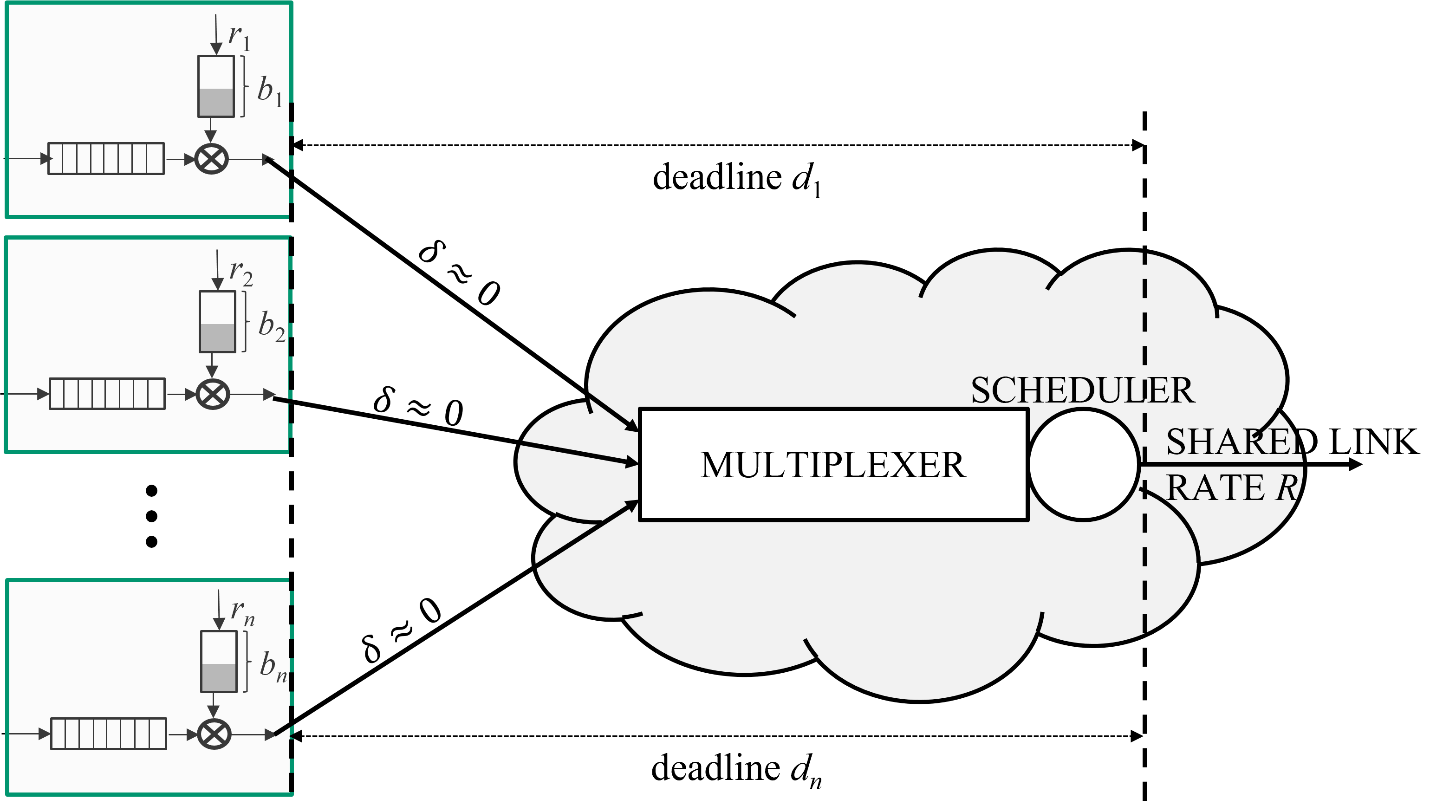
Refer to caption
Figure 1: A typical one-hop configuration with $n$ flows.

In this setting, let $\bm{r}=\left(r_{1},r_{2},\ldots,r_{n}\right)$, $\bm{b}=\left(b_{1},b_{2},\ldots,b_{n}\right)$, and $\bm{d}=\left(d_{1},d_{2},\ldots,d_{n}\right)$ be the vectors of rates, burst sizes, and deadlines of the flows sharing the link, respectively, and let $D^{*}_{i}(\bm{r},\bm{b},R)$ denote flow $i$’s worst-case delay (queueing+transmission). Our bandwidth minimization problem can then be formulated as an optimization of the form:

OPT_❏ $\displaystyle\min R$
s.t $\displaystyle D^{*}_{i}(\bm{r},\bm{b},R)\leq d_{i},$ $\displaystyle\forall i,1\leq i\leq n$

where $R$ is the optimization variable and ❏ denotes the scheduler type, which for notational simplicity has been omitted in the expression of $D^{*}_{i}(\bm{r},\bm{b},R)$. As mentioned in Section I, one of our goals is to evaluate the trade-off between (bandwidth) efficiency and complexity across different schedulers.

Another goal is to investigate the potential benefits of reprofiling flows prior to forwarding their traffic to the scheduler. Reprofiling amounts to applying a different, typically “smaller”, traffic profile to each flow before forwarding them to the scheduler. This can222When the reprofiler operates in a non-work-conserving manner. introduce an up-front reprofiling delay, but may lower the bandwidth required to meet overall latency goals if it makes flows “easier” to handle.

More formally, given a scheduler “” and $n$ flows sharing a link, where flow $i,1\leq i\leq n,$ has traffic profile $(r_{i},b_{i})$ and deadline $d_{i}$, the goal of reprofiling is to identify smaller burst sizes $b^{\prime}_{i}\leq b_{i},1\leq i\leq n,$ that minimize the link bandwidth $R$ needed to meet the flows’ deadlines, inclusive of any resulting reprofiling delay (the smaller burst $b^{\prime}_{i}$ introduces a reprofiling delay of $\frac{b_{i}-b^{\prime}_{i}}{r_{i}}$). We note that we restrict reprofiling options to only reducing the burst size, rather than also considering adding a “peak rate” shaper. This is in part to simplify the resulting optimization OPT_R❏, and also because, as shown in Appendix F, this is sufficient in simple configurations with only two flows. This translates into a modified optimization problem OPT_R❏ of the form

OPT_R❏ $\displaystyle\min_{\bm{b^{\prime}}}R$
s.t $\displaystyle D^{*}_{i}(\bm{r},\bm{b},\bm{b^{\prime}},R)\leq d_{i},$ $\displaystyle\forall i,1\leq i\leq n$

where $R$ and $\bm{b^{\prime}}$ are the optimization variables. The latter denotes the vectors of updated (reprofiled) burst sizes of the $n$ flows, and $D^{*}_{i}(\bm{r},\bm{b},\bm{b^{\prime}},R),1\leq i\leq n,$ are the worst case delays, accounting for reprofiling delays, of the $n$ flows under scheduler and a link bandwidth of $R$. The optimization explores the extent to which making flows smoother (smaller bursts) can facilitate meeting their delay targets with less bandwidth in spite of the access delay that reprofiling adds.

The next three sections explore solutions to OPT_❏ (and OPT_R❏) for different schedulers, namely, dynamic priority, static priority, and fifo (OPT_DP, OPT_SP, and OPT_F).

III Dynamic Priorities

We start with the most powerful but most complex scheduler, dynamic priorities, with priorities derived from service curves assigned to flows as a function of their profile (deadline and traffic envelope). We first solve OPT_DP by characterizing the service curves that achieve the lowest bandwidth while meeting all deadlines in the absence of any reprofiling.

To derive the result, we first specify a service-curve assignment $\Gamma_{sc}$ that satisfies all deadlines, identify the minimum link bandwidth $R^{*}$ required to realize $\Gamma_{sc}$, and show that any scheduler requires at least $R^{*}$. We then show that an earliest deadline first scheduler realizes $\Gamma_{sc}$ and, therefore, meets all the flow deadlines under $R^{*}$. e note that this then implies that reprofiling is of no benefit when an edf scheduler is available.

Proposition 1.

Consider a link shared by $n$ token bucket controlled flows, where flow $i,1\leq i\leq n$, has a traffic profile $(r_{i},b_{i})$ and a deadline $d_{i}$, with $d_{1}>d_{2}>...>d_{n}$ and $d_{1}<\infty$. Consider a service-curve assignment $\Gamma_{sc}$ that allocates flow $i$ a service curve of

SCi(t)={0 when t<di,bi+ri(tdi)otherwise.SC_{i}(t)=\left\{\begin{aligned} &0&\text{ when }t<d_{i},\\ &b_{i}+r_{i}(t-d_{i})&\text{otherwise}.\end{aligned}\right. (1)

Then

  1. 1.

    For any flow $i,1\leq i\leq n$, $SC_{i}(t)$ ensures a worst-case end-to-end delay no larger than $d_{i}$.

  2. 2.

    Realizing $\Gamma_{sc}$ requires a link bandwidth of at least

    $$R^{*}=\max_{1\leq h\leq n}\left\{\sum_{i=1}^{n}r_{i},\frac{\sum_{i=h}^{n}b_{i}+r_{i}(d_{h}-d_{i})}{d_{h}}\right\}.$$ (2)
  3. 3.

    Any scheduling mechanism capable of meeting all the flows’ deadlines requires a bandwidth of at least $R^{*}$.

The proof of Proposition 1 is in Appendix B-A. The optimality of $\Gamma_{sc}$ is intuitive. Recall that a service curve is a lower bound on the service received by a flow. Eq. (1) assigns service to a flow at a rate exactly equal to its input rate, but delayed by its deadline, i.e., provided at the latest possible time. Conversely, any mechanism $\widehat{\Gamma}$ that meets all flows’ deadlines must by time $t$ have provided flow $i$ a cumulative service at least equal to the amount of data that flow $i$ may have generated by time $t-d_{i}$, which is exactly $SC_{i}(t)$. Hence the mechanism must offer flow $i$ a service curve $\widehat{SC}_{i}(t)\geq SC_{i}(t),\forall t$.

Next, we identify at least one mechanism capable of realizing the services curves of Eq. (1) under $R^{*}$, and consequently providing a solution to OPT_DP for schedulers that support dynamic priorities.

Proposition 2.

Consider a link shared by $n$ token bucket controlled flows, where flow $i,1\leq i\leq n$, has traffic profile $(r_{i},b_{i})$ and deadline $d_{i}$, with $d_{1}>d_{2}>...>d_{n}$ and $d_{1}<\infty$. The earliest deadline first (edf) scheduler realizes $\Gamma_{sc}$ under a link bandwidth of $R^{*}$.

The proof of Proposition 2 is in Appendix B-B. We note that the optimality of edf is intuitive, as minimizing the required bandwidth is the dual problem to maximizing the schedulable region for which edf’s optimality is known [18].

As previously mentioned and as the next proposition formally states, reprofiling does not reduce the minimum required bandwidth $R^{*}$ of Eq. (2). Consequently, it affords no benefits with edf schedulers capable of meeting the deadlines under $R^{*}$. This is expected given the optimality of edf schedulers.

Proposition 3.

Consider a link shared by $n$ token bucket controlled flows, where flow $i,1\leq i\leq n$, has traffic profile $(r_{i},b_{i})$ and deadline $d_{i}$, with $d_{1}>d_{2}>...>d_{n}$ and $d_{1}<\infty$. Reprofiling flows will not decrease the minimum bandwidth required to meet the flows’ deadlines.

The proof is in Appendix B-C.

Note that $\Gamma_{sc}$ specifies a non-linear (piece-wise-linear) service curve for each flow. Given the popularity and simplicity of linear service curves, i.e., rate-based schedulers, it is tempting to investigate whether such schedulers, e.g., GPS [19], could be used instead. Unfortunately, it is easy to find scenarios where linear service curves perform worse.

Consider a link shared by two flows with traffic profiles $(r_{1},b_{1})=(1,45)$ and $(r_{2},b_{2})=(1,5)$, and deadlines $d_{1}=10$ and $d_{2}=1$. A rate-based scheduler must allocate a bandwidth of $\max\left\{\frac{b}{d},r\right\}$ to a flow with traffic profile $(r,b)$ to meet its deadline $d$ of. Applying this to flow $2$ that has the tighter deadline calls for a bandwidth of $5$ to meet its deadline. After $1.25$ units of time (the time to clear the initial burst of $5$ and the additional data that accumulated during its transmission), flow $2$’s bandwidth usage drops down to $r_{2}=1$. The remaining $4$ units then become available to flow $1$. This means that the initial dedicated bandwidth needed by flow $1$ to meet its deadline of $10$ given its burst size of $b_{1}=45$ is simply its token rate $r_{1}=1$333Clearing the burst of flow $1$ by its deadline $d_{1}=10$ calls for a bandwidth $x$ such that $45-\frac{5}{4}x-(x+4)\left(10-\frac{5}{4}\right)\leq 0$, which yields $x\geq 1$., for a total network bandwidth of $6$ units. In contrast, Eq. (2) tells us that $\Gamma_{sc}$, only requires a bandwidth of $R^{*}=5.9$.

The next two sections consider simpler static priority and fifo schedulers, and quantify the bandwidth they require to meet flows’ deadlines. Both schedulers are considered either alone or with “reprofilers” that first modify the flows’ traffic profiles before they are allowed to access the scheduler.

IV Static Priorities

Though edf schedulers are efficient and increasingly realizable [20, 21, 22], they are expensive and may not be practical in all environments. It is, therefore, of interest to explore simpler alternatives while quantifying the trade-off they entail between efficacy and complexity. For that purpose, we consider next a static priority scheduler where each flow is assigned a fixed priority as a function of its deadline.

As before, we consider $n$ flows with traffic profiles $(r_{i},b_{i})$ and deadlines $d_{i},1\leq i\leq n$, sharing a common link. The question we first address is how to assign (static) priorities to each flow given their deadlines and OPT_SP’s goal of minimizing link bandwidth? The next proposition offers a partial and somewhat intuitive answer to this question by establishing that the minimum link bandwidth can be achieved by giving flows with shorter deadlines a higher priority. Formally,

Proposition 4.

Consider a link shared by $n$ token bucket controlled flows, where flow $i,1\leq i\leq n$, has traffic profile $(r_{i},b_{i})$ and deadline $d_{i}$, with $d_{1}>d_{2}>...>d_{n}$ and $d_{1}<\infty$. Under a static-priority scheduler, there exists an assignment of flows to priorities that minimizes link bandwidth while meeting all flows deadlines such that flow $i$ is assigned a priority strictly greater than that of flow $j$ only if $d_{i}<d_{j}$.

The proof is in Appendix C-A. We note that while Proposition 4 states that link bandwidth can be minimized by assigning flows to priorities in the order of their deadline, it neither rules out other mappings nor does it imply that flows with different deadlines should always be mapped to distinct priorities. For example, large enough deadlines can all be met by a link bandwidth equal to the sum of the flows’ average rates, i.e., $R^{*}=\sum_{i=1}^{n}r_{i}$. In this case, priorities and their ordering are irrelevant. More generally, grouping flows with different deadlines in the same priority class can often result in a lower bandwidth than mapping them to distinct priority classes444We illustrate this in Appendix E for the case of two flows sharing a static priority scheduler.. Nevertheless, motivated by Proposition 4, we propose a simple assignment rule that strictly maps lower deadline flows to higher priorities, and evaluate its performance.

IV-A Static Priorities without Reprofiling

From [17, Proposition $1.3.4$] we know that when $n$ flows with traffic profiles $(r_{i},b_{i}),1\leq i\leq n$, share a link of bandwidth $R\geq\sum_{i=1}^{n}r_{i}$ with flow $i$ assigned to priority $i$ (priority $n$ is the highest), then, under a static-priority scheduler, the worst case delay of flow $h$ is upper-bounded by $\frac{\sum_{i=h}^{n}b_{i}}{R-\sum_{i=h+1}^{n}r_{i}}$ (recall that under our notation, priority $n$ is the highest). As a result, the minimum link bandwidth $\widetilde{R}^{*}$ to ensure that flow $h$’s deadline $d_{h}$ is met for all $h$, i.e., solving OPT_SP, is given by:

$$\widetilde{R}^{*}=\max_{1\leq h\leq n}\left\{\sum_{i=1}^{n}r_{i},\frac{\sum_{i=h}^{n}b_{i}}{d_{h}}+\sum_{i=h+1}^{n}r_{i}\right\}$$ (3)

Towards evaluating the performance of a static priority scheduler versus that of an edf scheduler, we compare $\widetilde{R}^{*}$ with $R^{*}$ through their relative difference, i.e., $\frac{\widetilde{R}^{*}-R^{*}}{R^{*}}$. For ease of comparison, we rewrite $R^{*}$ as

$$R^{*}=\max_{1\leq h\leq n}\left\{\sum_{i=1}^{n}r_{i},\frac{\sum_{i=h}^{n}b_{i}}{d_{h}}+\sum_{i=h+1}^{n}r_{i}\left(1-\frac{d_{i}}{d_{h}}\right)\right\}$$ (4)

Comparing Eqs. (3) and (4) shows that $R^{*}=\widetilde{R}^{*}$ iff $\widetilde{R}^{*}=\sum_{i=1}^{n}r_{i}$, i.e., $\frac{\sum_{i=h}^{n}b_{i}}{d_{h}}\leq\sum_{i=1}^{h}r_{i},\forall\ 1\leq h\leq n$. In other words, static priority and edf schedulers perform equally well (yield the same minimum bandwidth), when flow bursts are small and deadlines relatively large so that they can be met with a link bandwidth equal to the sum of the token rates. However, when $\widetilde{R}^{*}\neq\sum_{i=1}^{n}r_{i}$, a static priority scheduler can require a much larger bandwidth.

Consider a scenario where $R^{*}$ is achieved at $h^{*}$, i.e., $R^{*}=\frac{\sum_{i=h^{*}}^{n}b_{i}}{d_{h^{*}}}+\sum_{i=h^{*}+1}^{n}r_{i}\left(1-\frac{d_{i}}{d_{h^{*}}}\right)$. Though $\widetilde{R}^{*}$ may not be realized at the same $h^{*}$ value, this still provides a lower bound for $\widetilde{R}^{*}$, namely, $\widetilde{R}^{*}\geq\frac{\sum_{i=h^{*}}^{n}b_{i}}{d_{h^{*}}}+\sum_{i=h^{*}+1}^{n}r_{i}$. Thus, the relative difference between $\widetilde{R}^{*}$ and $R^{*}$ is no less than

$\displaystyle\frac{\frac{\sum_{i=h^{*}}^{n}b_{i}}{d_{h^{*}}}+\sum_{i=h^{*}+1}^{n}r_{i}}{\frac{\sum_{i=h^{*}}^{n}b_{i}}{d_{h^{*}}}+\sum_{i=h^{*}+1}^{n}r_{i}\left(1-\frac{d_{i}}{d_{h^{*}}}\right)}-1$
$\displaystyle=\frac{\sum_{i=h^{*}+1}^{n}d_{i}r_{i}}{\sum_{i=h^{*}}^{n}b_{i}\ +\sum_{i=h^{*}+1}^{n}r_{i}\left(d_{h^{*}}-d_{i}\right)}$ (5)

As the right-hand-side of Eq. (5) increases with $d_{i}$ for all $i\geq h^{*}$, it is maximized for $d_{i}=d_{h^{*}}-\epsilon_{i},\forall i>h^{*}$, for arbitrarily small $\epsilon_{h^{*}+1}<\ldots<\epsilon_{n}$, so that its supremum is equal to $\frac{\sum_{i=h^{*}+1}^{n}r_{i}d_{h^{*}}}{\sum_{i=h^{*}}^{n}b_{i}}$. Note that this is intuitive, as when flows have arbitrarily close deadlines, they should receive equal service shares, which is in direct conflict with a strict priority ordering.

Under certain flow profiles, the above supremum can be large. In a two-flow scenario, basic algebraic manipulations give a supremum of $\frac{r_{2}}{r_{1}+r_{2}}$, which is achieved at $d_{2}=d_{1}=\frac{b_{2}+b_{1}}{r_{1}+r_{2}}$. Since $\frac{r_{2}}{r_{1}+r_{2}}\to 1$ as $\frac{r_{1}}{r_{2}}\to 0$, the optimal static priority scheduler in the two-flow case could require twice as much bandwidth as the optimal edf scheduler.

IV-B Static Priorities with Reprofiling

Static priorities can require significantly more bandwidth than $R^{*}$ mostly because they are a rather blunt instrument when it comes to fine-tuning the allocation of transmission opportunities as a function of packet deadlines. In particular, they often result in some flows experiencing a delay much lower than their target deadline.

This is intrinsic to the static structure of the scheduler and to our choice of an assignment that maps distinct deadlines to different priorities, but can be mitigated by anticipating and leveraging the “slack” in the delay of some flows. One such option is to use this slack towards reprofiling those flows, i.e., make them “smoother”. Of interest then, is how to reprofile flows to maximize any resulting link bandwidth reduction?

Consider the trivial example of a single link shared by two flows with traffic profiles $(r_{1},b_{1})=(1,5)$ and $(r_{2},b_{2})=(4,5)$ and deadlines $d_{1}=1.4,d_{2}=1.25$. A strict static-priority scheduler requires a bandwidth $\widetilde{R}^{*}=11.14$. Assume next that we reprofile flow $2$ to $(r_{2},b^{\prime}_{2})=(4,0)$ before it enters the scheduler. The added reprofiling delay of $(b_{2}-b^{\prime}_{2})/r_{2}=1.25$ reduces the scheduling delay budget down to 00, but eliminates all burstiness. As a result, we only need a bandwidth of $7.57$ (under a fluid model) to meet both flows’ deadlines (a bandwidth of $4=r_{2}$ is still consumed by flow $2$, but the remaining $3.57$ is sufficient to allow flow $1$ to meet its deadline). In other words, reprofiling flow $2$ yields a bandwidth decrease of more than $30\%$. This simple example illustrates the benefits that judicious reprofiling can afford.

The next few propositions characterize the optimal reprofiling solution and the resulting bandwidth gains for a static priority scheduler and a set of flows and deadlines. We first derive expressions for flows’ reprofiling and scheduling delays under static priorities, before obtaining the optimal reprofiling solution and the resulting minimum link bandwidth $\widetilde{R}^{*}_{R}$.

Specifically, given $n$ flows with initial traffic profiles $(r_{i},b_{i}),1\leq i\leq n,$ deadlines $d_{1}>d_{2}>\ldots>d_{n},$ a reprofiling solution $(r_{i},b^{\prime}_{i}),1\leq i\leq n,$ and a link of bandwidth $R$, Proposition 5 characterizes the worst case delay (reprofiling plus scheduling) of each flow, when a static priority scheduler assigns flow $i$ priority $i$ (shorter deadlines have higher priority). The result is used to formulate an optimization problem, OPT_RSP, that seeks to minimize the link bandwidth required to meet individual flows’ deadlines. The variables of the optimization are the reprofiling solution and the link bandwidth. Proposition 7 characterizes the minimum bandwidth $\widetilde{R}^{*}_{R}$ that OPT_RSP can achieve, while Proposition 8 provides the optimal reprofiling solution.

Let $\bm{b}^{\prime}=(b^{\prime}_{1},b^{\prime}_{2},b^{\prime}_{3},...,b^{\prime}_{n})$ be the vector of reprofiled flow bursts, with $B^{\prime}_{i}=\sum_{j=i}^{n}b^{\prime}_{j}$ and $R_{i}=\sum_{j=i}^{n}r_{j}$, the sum of the reprofiled bursts and rates of flows with priority greater than or equal to $i,1\leq i\leq n$, where $B^{\prime}_{i}=0$ and $R_{i}=0$ for $i>n$. Flow $i$’s worst-case end-to-end delay is characterized next.

Proposition 5.

Consider a link shared by $n$ token bucket controlled flows, where flow $i,1\leq i\leq n$, has traffic profile $(r_{i},b_{i})$. Assume a static priority scheduler that assigns flow $i$ a priority of $i$, where priority $n$ is the highest priority, and reprofiles flow $i$ to $(r_{i},b^{\prime}_{i})$, where $0\leq b^{\prime}_{i}\leq b_{i}$. Given a link bandwidth of $R\geq\sum_{j=1}^{n}r_{j}$, the worst-case delay for flow $i$ is

$$D^{*}_{i}=\max\left\{\frac{b_{i}+B^{\prime}_{i+1}}{R-R_{i+1}},\ \frac{b_{i}-b^{\prime}_{i}}{r_{i}}+\frac{B^{\prime}_{i+1}}{R-R_{i+1}}\right\}.$$ (6)

The proof is in Appendix C-B. Note that Eq. (6) states that flow $i$’s worst-case delay is realized by the last bit of its burst. The two terms of Eq. (6) capture the cases when this bit arrives before or after the end of flow $i$’s last busy period at the link, respectively, as this determines the extent to which it is affected by the reprofiling delay.

Observe also that $D^{*}_{i}$ is independent of $b^{\prime}_{1}$ for $2\leq i\leq n$, and decreases with $b^{\prime}_{1}$ when $i=1$. This is intuitive as flow $1$ has the lowest priority so that reprofiling it can neither decrease the worst-case end-to-end delay of other flows, nor consequently reduce the minimum link bandwidth required to meet specific deadlines for each flow. Formally,

Corollary 6.

Consider a link shared by $n$ token bucket controlled flows, where flow $i,1\leq i\leq n$, has traffic profile $(r_{i},b_{i})$ and deadline $d_{i}$, with $d_{1}>d_{2}>...>d_{n}$ and $d_{1}<\infty$. Assume a static priority scheduler that assigns flow $i$ a priority of $i$, where priority $n$ is the highest priority, and reprofiles flow $i$ to $(r_{i},b^{\prime}_{i})$, where $0\leq b^{\prime}_{i}\leq b_{i}$. Given a link bandwidth of $R\geq\sum_{j=1}^{n}r_{j}$, reprofiling flow $1$ cannot reduce the minimum required bandwidth.

Combining Proposition 5 and Corollary 6 with OPT_SP gives the following optimization OPT_RSP for a link shared by $n$ flows and relying on a static priority scheduler preceded by reprofiling. Note that since the minimum link bandwidth needs to satisfy $R\geq\sum_{i=1}^{n}r_{i}$, combining this condition with $R_{i}$’s definition gives $\sum_{i=1}^{n}r_{i}=R_{1}\leq R$.

$\displaystyle\text{{OPT\_RSP}}\quad\min_{\bm{b}^{\prime}}R\quad\text{s.t}$
$\displaystyle\!\max\left\{\frac{b_{i}+B^{\prime}_{i+1}}{R-R_{i+1}},\frac{b_{i}-b^{\prime}_{i}}{r_{i}}+\frac{B^{\prime}_{i+1}}{R-R_{i+1}}\right\}\leq d_{i},\ \forall\ 1\leq i\leq n,$
$\displaystyle R_{1}\leq R,\quad b^{\prime}_{1}=b_{1},\quad 0\leq b^{\prime}_{i}\leq b_{i},\ \forall\ 2\leq i\leq n.$

The solution of OPT_RSP is characterized in Propositions 7 and 8 whose proofs are in Appendix C-C. Proposition 7 gives the optimal bandwidth $\widetilde{R}^{*}_{R}$ based only on flow profiles, and while it is too complex to yield a closed-form expression, it offers a feasible numerical procedure to compute $\widetilde{R}^{*}_{R}$.

Proposition 7.

For $1\leq i\leq n$, denote $H_{i}=b_{i}-d_{i}r_{i}$, $\Pi_{i}(R)=\frac{r_{i}+R-R_{i+1}}{R-R_{i+1}}$ and $V_{i}(R)=d_{i}(R-R_{i+1})-b_{i}$. Define $\mathbb{S}_{1}(R)=\left\{V_{1}(R)\right\}$, and $\mathbb{S}_{i}(R)=\mathbb{S}_{i-1}(R)\bigcup\left\{V_{i}(R)\right\}\bigcup\left\{\frac{s-H_{i}}{\Pi_{i}(R)}\ |\ s\in\mathbb{S}_{i-1}(R)\right\}$ for $2\leq i\leq n$. Then we have $\widetilde{R}^{*}_{R}=\max\left\{R_{1},\inf\{R\ |\ \forall s\in\mathbb{S}_{n}(R),s\geq 0\}\right\}$.

Computing $\widetilde{R}^{*}_{R}$ requires solving polynomial inequalities of degree $(n-1)$, so that a closed-form expression is not feasible except for small $n$. However, as $\mathbb{S}_{i}(R)$ relies only on flow profiles and $\mathbb{S}_{j}(R)$, $\forall j<i$, we can recursively construct $\mathbb{S}_{n}(R)$ from $\mathbb{S}_{1}(R)$. Hence, since $R_{1}\leq\widetilde{R}^{*}_{R}\leq\widetilde{R}^{*}$, we can use a binary search to compute $\widetilde{R}^{*}_{R}$ from the relation $\widetilde{R}^{*}_{R}=\max\left\{R_{1},\inf\{R\ |\ \forall s\in\mathbb{S}_{n}(R),s\geq 0\}\right\}$ in Proposition 7.

Next, Proposition 8 gives a constructive procedure to obtain the optimal reprofiling burst sizes $\bm{b}^{\prime*}$ given $\widetilde{R}^{*}_{R}$ and the original flow profiles.

Proposition 8.

The optimal reprofiling solution $\bm{b}^{\prime*}$ satisfies

$$b^{\prime*}_{i}=\left\{\begin{aligned} &\max\{0,b_{n}-r_{n}d_{n}\},&i=n;\qquad\quad\,\,\,\\ &\max\left\{0,b_{i}-r_{i}d_{i}+\frac{r_{i}B^{\prime*}_{i+1}}{\widetilde{R}^{*}_{R}-R_{i+1}}\right\},&2\leq i\leq n-1.\end{aligned}\right.$$ (7)

where we recall that $b^{\prime*}_{1}=b_{1}$ and $B^{\prime*}_{i}=\sum_{j=i}^{n}b^{\prime*}_{j}$.

Note that the optimal reprofiling burst size $b^{\prime*}_{i}$ of flow $i,1<i<n$ relies only on the optimal link bandwidth $\widetilde{R}^{*}_{R}$ and the reprofiling burst sizes of higher priority flows. Hence, we can recursively characterize $b^{\prime*}_{i}$ from $b^{\prime*}_{n}$ given $\widetilde{R}^{*}_{R}$.

V Basic FIFO with Reprofiling

In this section, we consider a simple first-in-first-out (fifo) scheduler that serves data in the order in which it arrives. For conciseness and given the benefits of reprofiling demonstrated in Section IV-B, we directly assume that flows are reprofiled prior to being scheduled. Considering again a link shared by $n$ flows with traffic profiles $(r_{i},b_{i}),1\leq i\leq n,$ and deadlines $d_{1}>d_{2}>\ldots>d_{n},$ our goal is to find a reprofiling solution $(r_{i},b^{\prime}_{i}),$ $1\leq i\leq n,$ to minimize the link bandwidth required to meet the flows’ deadlines.

Towards answering this question, we first proceed to characterize the worst case delay across $n$ flows sharing a link of bandwidth $R$ equipped with a fifo scheduler when the flows have initial traffic profiles $(r_{i},b_{i}),1\leq i\leq n,$ and are reprofiled to $(r_{i},b^{\prime}_{i}),1\leq i\leq n,$ prior to being scheduled. Using this result, we then identify the reprofiled burst sizes $b^{\prime}_{i},1\leq i\leq n,$ that minimize the link bandwidth required to ensure that all deadlines $d_{1}>d_{2}>\ldots>d_{n},$ and $d_{1}<\infty$ are met. As with other configurations, we only state the results with proofs relegated to Appendix D.

Proposition 9.

Consider a system with $n$ token bucket controlled flows with traffic profiles $(r_{i},b_{i}),1\leq i\leq n$, sharing a fifo link with bandwidth $R\geq R_{1}=\sum_{j=1}^{n}r_{j}$. Assume that the system reprofiles flow $i$ to $(r_{i},b^{\prime}_{i})$. The worst-case delay for flow $i$ is then

$$\widehat{D}^{*}_{i}=\max\left\{\frac{b_{i}-b^{\prime}_{i}}{r_{i}}+\frac{\sum_{j\neq i}b^{\prime}_{j}}{R},\frac{\sum_{j=1}^{n}b^{\prime}_{j}}{R}+\frac{(b_{i}-b^{\prime}_{i})R_{1}}{r_{i}R}\right\}.$$ (8)

The proof of Proposition 9 is in Appendix D-A.

With the result of Proposition 9 in hand, we can formulate a corresponding optimization problem, OPT_RF, for computing the optimal reprofiling solution that minimizes the link bandwidth required to meet the deadlines $d_{1}>d_{2}>\ldots>d_{n},$ and $d_{1}<\infty$ of the $n$ flows. Specifically, combining Proposition 9 with OPT_F gives the following optimization OPT_RF for a link shared by $n$ flows when relying on a fifo scheduler preceded by reprofiling. As before, $\sum_{i=1}^{n}r_{i}=R_{1}\leq R$.

$\displaystyle\text{{OPT\_RF}}\quad\min_{\bm{b}^{\prime}}R\quad\text{s.t}\quad\forall\ 1\leq i\leq n$ (9)
$\displaystyle\max\left\{\frac{b_{i}-b^{\prime}_{i}}{r_{i}}+\frac{\sum_{j\neq i}b^{\prime}_{j}}{R},\frac{\sum_{j=1}^{n}b^{\prime}_{j}}{R}+\frac{(b_{i}-b^{\prime}_{i})R_{1}}{r_{i}R}\right\}\leq d_{i},$
$\displaystyle R_{1}\leq R,\quad 0\leq b^{\prime}_{i}\leq b_{i},\forall\ 1\leq i\leq n.$

The solution of OPT_RF is characterized in Propositions 10 and 11 with proofs in Appendix D-B. As with a static priority scheduler, Proposition 10 gives a numerical procedure to compute the optimal bandwidth $\widehat{R}^{*}_{R}$ given the flows’ profiles, while Proposition 11 gives the optimal reprofiling solution $\bm{\widehat{b}}^{\prime*}$ given $\widehat{R}^{*}_{R}$ and the original flows’ profiles.

Proposition 10.

For $1\leq i\leq n$, define $H_{i}=b_{i}-d_{i}r_{i}$, $\widehat{B}_{i}=\sum_{j=1}^{i}b_{j}$, and $\mathbb{Z}_{i}=\{1\leq j\leq i\mid j\in\mathbb{Z}\}$. Denote

$$X_{F}(R)=\!\!\!\max_{\begin{subarray}{c}P_{1},P_{2}\subseteq\mathbb{Z}_{n},\\ P_{2}\neq\mathbb{Z}_{n},P_{1}\bigcap P_{2}=\emptyset\end{subarray}}\!\!\!\frac{\sum_{i\in P_{1}}\frac{RH_{i}}{R+r_{i}}+\sum_{i\in P_{2}}\left(b_{i}-\frac{r_{i}d_{i}R}{R_{1}}\right)}{1-\sum_{i\in P_{1}}\frac{r_{i}}{R+r_{i}}-\sum_{i\in P_{2}}\frac{r_{i}}{R_{1}}}$$

and

$\displaystyle Y_{F}(R)$ =min1in1\bBigg@3{B^n,Rdn,\displaystyle=\min_{1\leq i\leq n-1}\bBigg@{3}\{\widehat{B}_{n},Rd_{n},
$\displaystyle\min_{\begin{subarray}{c}P_{1},P_{2}\subseteq\mathbb{Z}_{i},\\ P_{1}\bigcap P_{2}=\emptyset,\\ P_{1}\bigcup P_{2}\neq\emptyset\end{subarray}}$ $\displaystyle\left.\left\{\frac{\widehat{B}_{i}-\sum_{j\in P_{1}}\frac{RH_{j}}{R+r_{j}}-\sum_{j\in P_{2}}\left(b_{j}-\frac{r_{j}d_{j}R}{R_{1}}\right)}{\sum_{j\in P_{1}}\frac{r_{j}}{R+r_{j}}+\sum_{j\in P_{2}}\frac{r_{j}}{R_{1}}}\right\}\right\}.$

Then the optimal solution for OPT_RF is

$$\widehat{R}^{*}_{R}=\max\left\{R_{1},\frac{\widehat{B}_{n}R_{1}}{\sum_{i=1}^{n}r_{i}d_{i}},\min\{R\mid X_{F}(R)\leq Y_{F}(R)\}\right\}.$$

As $\max\left\{R_{1},\frac{\widehat{B}_{n}R_{1}}{\sum_{i=1}^{n}r_{i}d_{i}}\right\}\leq\widehat{R}^{*}_{R}\leq\widehat{R}^{*}=\max\left\{R_{1},\frac{\widehat{B}_{n}}{d_{n}}\right\}$, where $\widehat{R}^{*}$ is the minimum required bandwidth achieved by a base (no reprofiling) fifo system, we can use Proposition 10 and a binary search to compute $\widehat{R}^{*}_{R}$. Once $\widehat{R}^{*}_{R}$ is known, Proposition 11 gives the optimal reprofiling solution.

Proposition 11.

For $1\leq i\leq n$, define $T_{i}(\widehat{B}^{\prime}_{n},R)=\max\left\{0,\frac{R}{R+r_{i}}\left(H_{i}+\frac{r_{i}}{R}\widehat{B}^{\prime}_{n}\right),b_{i}+\frac{r_{i}(\widehat{B}^{\prime}_{n}-Rd_{i})}{R_{1}}\right\}$. The optimal reprofiling solution $\bm{\widehat{b}}^{\prime*}$ of OPT_RF’s is given by $\widehat{b}^{\prime*}_{1}=\widehat{B}^{\prime*}_{1}$, and $\widehat{b}^{\prime*}_{i}=\widehat{B}^{\prime*}_{i}-\widehat{B}^{\prime*}_{i-1}$, $2\leq i\leq n$, where $\bm{\widehat{B}}_{i}^{\prime*}$ satisfy

$$\left\{\begin{aligned} &\widehat{B}^{\prime*}_{n}=X_{F}(\widehat{R}^{*}_{R}),\\ &\widehat{B}^{\prime*}_{i}=\max\left\{\sum_{j=1}^{i}T_{j}(\widehat{B}^{\prime*}_{n},\widehat{R}^{*}_{R}),\widehat{B}^{\prime*}_{i+1}-b_{i+1}\right\},\\ &\text{ when }1\leq i\leq n-1.\end{aligned}\right.$$ (10)

Note that $\widehat{B}^{\prime*}_{n}$ relies only on $\widehat{R}^{*}_{R}$ and flows’ profiles. Whereas when $1\leq i\leq n-1$, $\widehat{B}^{\prime*}_{i}$ relies only on $\widehat{R}^{*}_{R}$, $\widehat{B}^{\prime*}_{n}$, $\widehat{B}^{\prime*}_{i+1}$ and flows’ profiles. Hence, we can recursively characterize $\widehat{B}^{\prime*}_{i}$ from $\widehat{B}^{\prime*}_{n}$ given $\widehat{R}^{*}_{R}$.

VI Evaluation

In this section, we explore the relative benefits of the solutions developed in the previous three sections. Of interest is assessing the “cost of simplicity,” namely, the amount of additional bandwidth required by simpler schedulers such as static priority or fifo compared to an edf scheduler. Also of interest is the magnitude of the improvements that reprofiling affords with static priority and fifo schedulers. To that end, the evaluation proceeds with a number of pairwise comparisons to quantify the relative (bandwidth) cost of each alternative.

The evaluation first focuses (Section VI-A) on scenarios with just two flows. Closed-form expressions are then available for the minimum bandwidth of each configuration, which make formal comparisons possible. Section VI-B extends this to more “general” scenarios involving multiple flows with different combinations of deadlines and traffic profiles.

In the initial two-flow comparisons of Section VI-A, we first select a pair of representative traffic profiles (token buckets), and then vary the flows’ respective deadlines over a wide range of values. For each such combination, we explicitly compute the relative differences in bandwidth required by the different schedulers (with and without reprofiling, as applicable) using expressions derived from the propositions obtained in the previous sections. The results are presented in the form of “heat-maps” across the range of deadline combinations.

For the more general scenarios involving multiple flows (Section VI-B), we first generate a set of flow profiles, i.e., token buckets and deadlines, by randomly selecting them from within specified ranges. For each such combination, the amount of bandwidth required to meet the flows’ deadlines are then computed using again results from the propositions derived in the previous sections. Finally, for each pair of schedulers, we report statistics (means, standard deviations and the $95\%$ confidence intervals of the means) of the relative bandwidth differences across those random selections.

VI-A Basic Two-Flow Configurations

Recalling our earlier notation for the minimum bandwidth in each configuration, i.e., $R^{*}$ (edf); $\widetilde{R}^{*}$ (static priority); $\widetilde{R}^{*}_{R}$ (static priority w/ reprofiling); $\widehat{R}^{*}$ (fifo); and $\widehat{R}^{*}_{R}$ (fifo w/ reprofiling), and specializing Eq. (2) to a configuration with two flows, $(r_{1},b_{1})$ and $(r_{2},b_{2})$, the absolute minimum bandwidth to meet the flows’ deadlines $d_{1}$ and $d_{2}$ is given by

$$R^{*}=\max\left\{r_{1}+r_{2},\ \frac{b_{2}}{d_{2}},\ \frac{b_{1}+b_{2}-r_{2}d_{2}}{d_{1}}+r_{2}\right\},$$ (11)

which is then also the bandwidth required by the edf scheduler.

Similarly, if we consider a static priority scheduler, from Eq. (3), its bandwidth requirement $\widetilde{R}^{*}$ (in the absence of any reprofiling) for the same two-flow configuration is of the form

$$\widetilde{R}^{*}=\max\left\{r_{1}+r_{2},\ \frac{b_{2}}{d_{2}},\ \frac{b_{1}+b_{2}}{d_{1}}+r_{2}\right\};$$ (12)

If (optimal) reprofiling is introduced, specializing Proposition 7 to two flows, the minimum bandwidth $\widetilde{R}^{*}_{R}$ reduces to

$\displaystyle\max\left\{r_{1}+r_{2},\frac{b_{2}}{d_{2}},\frac{b_{1}+b_{2}-r_{2}d_{2}}{d_{1}}+r_{2}\right\},\text{ when }\frac{b_{2}}{r_{2}}\geq\frac{b_{1}}{r_{1}}$ (13)
$\displaystyle\max\left\{r_{1}+r_{2},\frac{b_{2}}{d_{2}},\frac{b_{1}+\max\left\{b_{2}-r_{2}d_{2},0\right\}}{d_{1}}+r_{2}\right\},$
$\displaystyle\text{ otherwise};$

Finally, specializing the results of Propositions 10 and 11 to two flows, we find that the minimum required bandwidth $\widehat{R}^{*}$ under fifo without reprofiling is

$$\widehat{R}^{*}=\max\left\{r_{1}+r_{2},\ \frac{b_{1}+b_{2}}{d_{2}}\right\};$$ (14)

and that when (optimal) reprofiling is used, $\widehat{R}^{*}_{R}$ is given by Eq. (15).

$$\widehat{R}^{*}_{R}=\max\left\{r_{1}+r_{2},\frac{b_{2}}{d_{2}},\frac{(b_{1}+b_{2})(r_{1}+r_{2})}{d_{1}r_{1}+d_{2}r_{2}},\frac{b_{1}+b_{2}-d_{1}r_{1}+\sqrt{(b_{1}+b_{2}-d_{1}r_{1})^{2}+4r_{1}d_{2}b_{2}}}{2d_{2}}\right\}.$$ (15)

With these expressions in hand, we can now assess the relative benefits of each option in this two-flow scenario.

Specifically, we consider next combinations consisting of two flows with representative token bucket parameters $(r_{1},b_{1})=(4,10)$ and $(r_{2},b_{2})=(10,18)$, and systematically vary their respective deadlines $d_{1}\geq d_{2}$ over a range of values. The bandwidth required to meet the deadlines is then compared for different pairs of schedulers using the expressions reported in Eq. (11), Eq. (13), and Eq. (15).

VI-A1 The Impact of Scheduler Complexity

We first evaluate the impact of relying on schedulers of decreasing complexity, when those schedulers are coupled with an optimal reprofiling solution. In other words, we compare the bandwidth requirements of an edf scheduler to those of static priority and fifo schedulers combined with an optimal reprofiler. The comparison is in the form of relative differences (improvements realizable from more complex schedulers), i.e., $\frac{\widetilde{R}^{*}_{R}-R^{*}}{\widetilde{R}^{*}_{R}}$, $\frac{\widehat{R}^{*}_{R}-R^{*}}{\widehat{R}^{*}_{R}}$, and $\frac{\widehat{R}^{*}_{R}-\widetilde{R}^{*}_{R}}{\widehat{R}^{*}}$.

edf vs. static priority w/ optimal reprofiling.

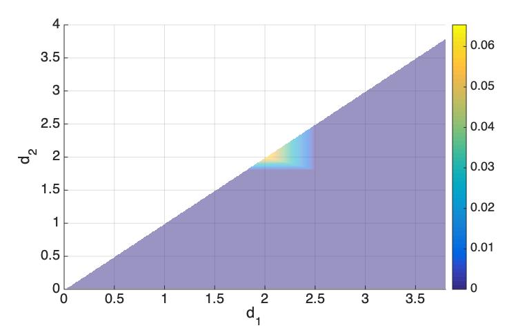
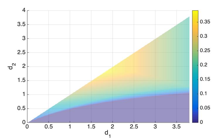
We start with comparing an edf scheduler with a static priority scheduler plus optimal reprofiling. Eqs. (11) and (13) then state that $R^{*}<\widetilde{R}^{*}_{R}$ iff $\frac{b_{2}}{r_{2}}<d_{2}\leq d_{1}<\frac{b_{1}}{r_{1}}$.

The results are reported in Fig. 2(a), and, as mentioned, are in the form of a heat-map of the relative bandwidth differences as the flows’ respective deadlines vary. As shown in the figure, a static priority scheduler, when combined with reprofiling, performs as well as an edf scheduler, except for a relatively small (triangular) region where $d_{1}$ and $d_{2}$ are close to each other and both of intermediate values555(i) When $d_{2}$ and $d_{1}$ are close and small, the bandwidth required to meet the deadlines is very large under either edf or static priority schedulers. This ensures that both produce similar transmissions’ orders. Consider, for example, a low-priority (larger deadline) burst that arrives $(d_{1}-d_{2})$ before a high-priority (smaller deadline) one. It has higher priority under edf, and the speed of the link ensures it is transmitted before the arrival of the high-priority burst, which ensures no difference between edf and a static priority scheduler.
(ii) When d2subscript𝑑2d_{2} and d1subscript𝑑1d_{1} are close but large, both schedulers meet their deadlines with the same bandwidth, i.e., the sum of the flows’ average rates.
. Towards better characterizing this range, i.e., d2>b2r2subscript𝑑2subscript𝑏2subscript𝑟2d_{2}>\frac{b_{2}}{r_{2}} and d1<b1r1subscript𝑑1subscript𝑏1subscript𝑟1d_{1}<\frac{b_{1}}{r_{1}}, we see that the supremum of R~RRR~Rsubscriptsuperscript~𝑅𝑅superscript𝑅subscriptsuperscript~𝑅𝑅\frac{\widetilde{R}^{*}_{R}-R^{*}}{\widetilde{R}^{*}_{R}} is achieved at d1=d2=b1+b2r1+r2subscript𝑑1subscript𝑑2subscript𝑏1subscript𝑏2subscript𝑟1subscript𝑟2d_{1}=d_{2}=\frac{b_{1}+b_{2}}{r_{1}+r_{2}}, with R~R=b1d1+r2subscriptsuperscript~𝑅𝑅subscript𝑏1subscript𝑑1subscript𝑟2\widetilde{R}^{*}_{R}=\frac{b_{1}}{d_{1}}+r_{2}, and R=r1+r2superscript𝑅subscript𝑟1subscript𝑟2R^{*}=r_{1}+r_{2}. The relative difference in bandwidth between the two schemes is then of the form

$$\frac{\widetilde{R}^{*}_{R}-R^{*}}{\widetilde{R}^{*}_{R}}=1-\frac{1}{\frac{b_{1}}{b_{1}+b_{2}}+\frac{r_{2}}{r_{1}+r_{2}}},$$

which can be shown to be upper-bounded by $0.5$. In other words, in the two-flow case, the (optimal) edf scheduler can result in a bandwidth saving of at most $50\%$ when compared to a static priority scheduler with (optimal) reprofiling. This happens when the deadlines of the two flows are very close to each other, a scenario unlikely in practice.

Refer to caption
(a) Dyn. prio. vs. stat. prio. + reprofiling
Refer to caption
(b) Dyn. prio. vs. fifo + reprofiling
Refer to caption
(c) fifo + reprofiling vs. stat. prio. + reprofiling
Figure 2: Relative bandwidth increases for $(r_{1},b_{1})=(4,10)$ and $(r_{2},b_{2})=(10,18)$, as a function of $d_{1}$ and $d_{2}<d_{1}$. The figure is in the form of a heat-map. Darker colors (purple) correspond to smaller increases than lighter ones (yellow).

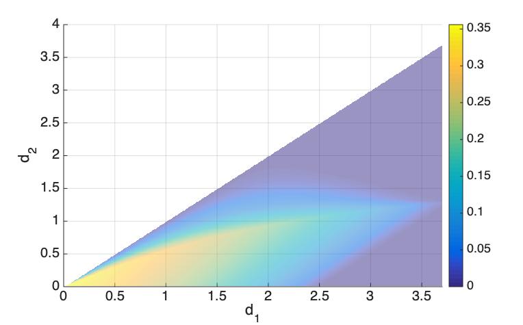
edf vs. fifo w/ optimal reprofiling

Next, we compare an edf scheduler and a fifo scheduler plus optimal reprofiling. Eqs. (11) and (15) state that $\widehat{R}^{*}_{R}>R^{*}$ iff $d_{1}-\frac{b_{1}}{r_{1}}<d_{2}<\frac{b_{1}+b_{2}-d_{1}r_{1}}{r_{2}}$. We illustrate the corresponding relative differences in Fig. 2(b) using the same two-flow combination as before. From the figure, we see that fifo + reprofiling performs poorly relative to an edf scheduler when neither $d_{1}$ nor $d_{2}$ are large. As with static priorities, such configurations may not be common in practice.

We note that the supremum of $\frac{\widehat{R}^{*}_{R}-R^{*}}{\widehat{R}^{*}_{R}}$ is achieved when $0<d_{2}<\frac{b_{1}+b_{2}+r_{2}d_{1}-\sqrt{(b_{1}+b_{2}+r_{2}d_{1})^{2}-4r_{2}b_{2}d_{1}}}{2r_{2}}$, with Eq. (11) defaulting to $R^{*}=\frac{b_{2}}{d_{2}}$ and Eq. (15) to $\widehat{R}^{*}_{R}=\frac{b_{1}+b_{2}-d_{1}r_{1}+\sqrt{(b_{1}+b_{2}-d_{1}r_{1})^{2}+4r_{1}d_{2}b_{2}}}{2d_{2}}$. Hence, the relative difference becomes

$\displaystyle\frac{\widehat{R}^{*}_{R}-R^{*}}{\widehat{R}^{*}_{R}}$ $\displaystyle=1$
$\displaystyle-$ $\displaystyle\frac{2b_{2}}{b_{1}+b_{2}-d_{1}r_{1}+\sqrt{(b_{1}+b_{2}-d_{1}r_{1})^{2}+4r_{1}d_{2}b_{2}}},$

which increases with $d_{2}$. Thus, its supremum is achieved as $d_{2}\to d_{1}$. Similarly, one easily shows that $1-\frac{2b_{2}}{b_{1}+b_{2}-d_{1}r_{1}+\sqrt{(b_{1}+b_{2}-d_{1}r_{1})^{2}+4r_{1}d_{2}b_{2}}}$ decreases with $d_{1}$. Hence, the supremum of the relative difference is achieved as $d_{1}\to 0$, and is of the form $\frac{b_{1}}{b_{1}+b_{2}}$, which goes to $1$ as $\frac{b_{1}}{b_{2}}\to\infty$. In other words, an edf scheduler can yield a $100\%$ improvement over a fifo scheduler with optimal reprofiling.

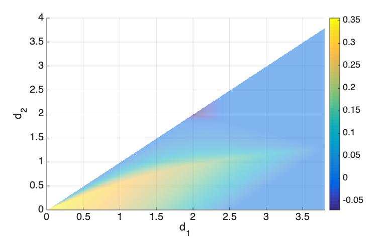
Fifo vs. static priority both w/ optimal reprofiling

Finally, we compare fifo and static priority schedulers when both rely on optimal reprofiling. Eqs. (13) and (15) give that $\widehat{R}^{*}_{R}>\widetilde{R}^{*}_{R}$ iff $\max\left\{\frac{b_{2}}{r_{2}},\frac{(b_{1}+b_{2})(r_{1}+r_{2})}{r_{2}(b_{1}/d_{1}+r_{2})}\right\}<d_{1}<\frac{b_{1}}{r_{1}}$. Fig. 2(c) illustrates the difference, again relying on a heat-map for the same two-flow combination as the two previous scenarios.

The figure shows that the benefits of priority are maximum when $d_{2}$ is small and $d_{1}$ is not too large. This is intuitive in that a small $d_{2}$ calls for affording maximum protection to flow $2$, which a priority structure offers more readily than a fifo. Conversely, when $d_{1}$ is large, flow $1$ can be reprofiled to eliminate all burstiness, which limits its impact on flow $2$ even when both flows compete in a fifo scheduler.

The figure also reveals that a small region exists (when $d_{1}$ and $d_{2}$ are close to each other and both are of intermediate value) where fifo outperforms static priority. As alluded to in the discussion following Proposition 4 and as expanded in Appendix E, this is because a strict priority ordering of flows as a function of their deadlines needs not always be optimal. For instance, it is easy to see that two otherwise identical flows that only differ infinitesimally in their deadlines should be treated “identically.” This is more readily accomplished by having them share a common fifo queue than assigned to two distinct priorities.

To better understand differences in performance between the two schemes, we characterize the supremum and the infimum of $\frac{\widehat{R}^{*}_{R}-\widetilde{R}^{*}_{R}}{\widehat{R}^{*}_{R}}$. Basic algebraic manipulations show that the supremum is achieved as $d_{1}=d_{2}\to 0$, where Eq. (15) defaults to $\widehat{R}^{*}_{R}=\frac{b_{1}+b_{2}-d_{1}r_{1}+\sqrt{(b_{1}+b_{2}-d_{1}r_{1})^{2}+4r_{1}d_{2}b_{2}}}{2d_{2}}$ and Eq. (13) to $\widetilde{R}^{*}_{R}=\frac{b_{2}}{d_{2}}$, so that their relative difference is ultimately of the form

$$\frac{\widehat{R}^{*}_{R}-\widetilde{R}^{*}_{R}}{\widehat{R}^{*}_{R}}=\frac{b_{1}}{b_{1}+b_{2}},$$

which goes to $1$ as $\frac{b_{1}}{b_{2}}\to\infty$, i.e., a maximum penalty of $100\%$ for fifo with reprofiling over static priorities with reprofiling.

Conversely, the infimum is achieved at $d_{1}=d_{2}=\frac{b_{1}+b_{2}}{r_{1}+r_{2}}$, with Eqs. (13) and (15) defaulting to $\widetilde{R}^{*}_{R}=\frac{b_{1}}{d_{1}}+r_{2}$ and $\widehat{R}^{*}_{R}=r_{1}+r_{2}$, and a relative difference of the form

$$\frac{\widehat{R}^{*}_{R}-\widetilde{R}^{*}_{R}}{\widehat{R}^{*}_{R}}=\frac{r_{1}}{r_{1}+r_{2}}-\frac{b_{1}}{b_{1}+b_{2}},$$

which increases with $\frac{r_{1}}{r_{2}}$ and decreases with $\frac{b_{1}}{b_{2}}$. When $\frac{r_{1}}{r_{2}}\to 0$ and $\frac{b_{1}}{b_{2}}\to\infty$, it achieves an infimum of $-1$, i.e., a maximum penalty of $100\%$ but now for static priorities with reprofiling over fifo with reprofiling. In other words, when used with reprofiling, both fifo and static priority can require twice as much bandwidth as the other.

Ensuring that static priority always outperforms fifo calls for determining when flows should be grouped in the same priority class rather than assigned to separate classes. Such grouping can be identified in simple scenarios with two or three flows, e.g., see Appendix E, but a general solution appears challenging. However, as we shall see in Section VI-B, the simple strict priority assignment on which we rely performs well in practice across a broad range of flow configurations.

VI-A2 The Benefits of Reprofiling

In this section, we evaluate the benefits afforded by (optimally) reprofiling flows with static priority and fifo schedulers. This is done by computing for both schedulers the minimum bandwidth required to meet flows’ deadlines without and with reprofiling, and evaluating the resulting relative differences, i.e., $\frac{\widetilde{R}^{*}-\widetilde{R}^{*}_{R}}{\widetilde{R}^{*}}$ and $\frac{\widehat{R}^{*}-\widehat{R}^{*}_{R}}{\widehat{R}^{*}}$.

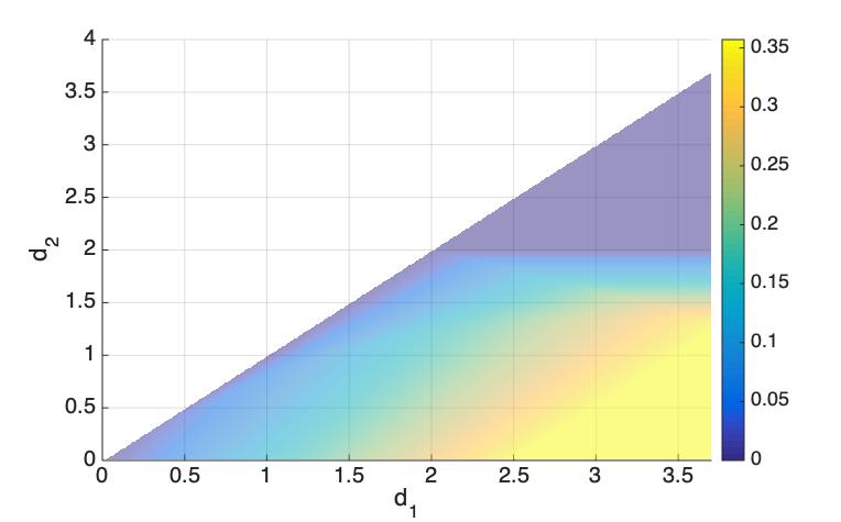
For a static priority scheduler, Eqs. (12) and (13) indicate that $\widetilde{R}^{*}_{R}<\widetilde{R}^{*}$ iff $\widetilde{R}^{*}=\frac{b_{1}+b_{2}}{d_{1}}+r_{2}>\max\left\{r_{1}+r_{2},\frac{b_{2}}{d_{2}}\right\}$, i.e., for a static priority scheduler, reprofiling666Recall from Corollary 6 that the flow with the largest deadline, flow $1$ in the two-flow case, is never reprofiled. decreases the required bandwidth only when $d_{1}$, the larger deadline, is not too large and $d_{2}$, the smaller deadline, is not too small. This is intuitive. When $d_{1}$ is large, the low-priority flow $1$ can meet its deadline even without any mitigation of the impact of flow $2$. Conversely, a small $d_{2}$ offers little to no opportunity for reprofiling flow $2$ as the added delay it introduces would need to be compensated by an even higher link bandwidth. This is illustrated in Fig. 3(a) for the same two-flow combination as in Fig. 2, i.e., $(r_{1},b_{1})=(4,10)$ and $(r_{2},b_{2})=(10,18)$. The intermediate region where “$d_{1}$ is not too large and $d_{2}$ is not too small” corresponds to the yellow triangular region where the benefits of reprofiling can reach $40\%$.

Refer to caption
(a) Stat. prio. without vs. with reprofiling
Refer to caption
(b) fifo without vs. with reprofiling
Figure 3: Relative bandwidth increases for $(r_{1},b_{1})=(4,10)$ and $(r_{2},b_{2})=(10,18)$ as a function of $d_{1}$ and $d_{2}<d_{1}$. The figure is in the form of a heat-map. Darker colors (purple) correspond to smaller increases than lighter ones (yellow).

Similarly, Eqs. (14) and (15) indicate that $\widehat{R}^{*}_{R}<\widehat{R}^{*}$ iff $d_{2}<\frac{b_{1}+b_{2}}{r_{1}+r_{2}}$, i.e., for a fifo scheduler, reprofiling decreases the required bandwidth only when $d_{2}$, the smaller deadline, is small. This is again intuitive as a large $d_{2}$ means that the deadline can be met even without reprofiling flow $1$777Note that under static priority the smaller deadline flow is reprofiled, while in the fifo case it is the larger deadline flow that is reprofiled to minimize its impact on the one with the tighter deadline.. Fig. 3(b) presents the relative gain in bandwidth for again the same 2-flow combination. As in the static priority case, the figure shows that for a fifo scheduler the benefits of reprofiling can reach about $40\%$ in the example under consideration.

The next section explores scenarios involving combinations of multiple flow profiles. Based on those results it appears that, unsurprisingly, a fifo scheduler stands to generally benefit more from reprofiling than a static priority one.

VI-B Relative Performance – Multiple Flows

In this section, we extend the investigation to configurations with more than two flows, using both synthetic flow profiles and profiles derived from datacenter traffic traces. The evaluation relies on generating a set of flow profiles, i.e., token buckets plus deadlines, and for each combination compute the bandwidth required to meet the deadlines using the results derived in the paper. The main difference with the 2-flow configurations of Section VI-A is that, as described next, we now consider a wider range of token bucket parameters with different possible combinations of deadlines. Additionally, unlike the 2-flow configurations for which the amount of bandwidth required could be obtained from explicit expressions, i.e., Eq. (11), Eq. (13), and Eq. (15), computing the required bandwidth now typically involves numerical procedures, as documented in the propositions derived in the paper.

VI-B1 Synthetic Flow Profiles

We assign flows to ten different deadline classes with a dynamic range of $10$, i.e., with minimum and maximum deadlines of $0.1$ and $1$, respectively, and consider different spreads in that range for the $10$ deadlines classes. Specifically, we select three different possible types of spreads for deadline classes, namely,
Even deadline spread:

  1. 1.

    $\bm{d}_{11}=(1,0.9,0.8,0.7,0.6,0.5,0.4,0.3,0.2,0.1)$;

Bi-modal deadline spread:

  1. 2.

    $\bm{d}_{21}=(1,0.95,0.9,0.85,0.8\|0.3,0.25,0.2,0.15,0.1)$,

  2. 3.

    $\bm{d}_{22}=(1,0.96,0.93,0.9,0.86,0.83,0.8\|0.2,0.15,0.1)$,

  3. 4.

    $\bm{d}_{23}=(1,0.95,0.9\|0.3,0.26,0.23,0.2,0.16,0.13,0.1)$;

Tri-modal deadline spread:

  1. 5.

    $\bm{d}_{31}=(1,0.95,0.9\|0.6,0.55,0.5,0.45\|0.2,0.15,0.1)$,

  2. 6.

    $\bm{d}_{32}=(1\|0.68,0.65,0.62,0.6,0.57,0.55,0.53,0.5\|0.1)$,

  3. 7.

    $\bm{d}_{33}=(1\|0.6\|0.28,0.25,0.23,0.2,0.17,0.15,0.12,0.1)$,

  4. 8.

    $\bm{d}_{34}=(1,0.97,0.95,0.93,0.9,0.88,0.85,0.82\|0.6\|0.1)$.

Those three types of spreads translate into different groupings of deadlines, which affect the relative numbers of deadlines in close proximity to each others.

Each of the above eight groupings is used across $1,000$ experiments, where an experiment consists of randomly selecting a “flow’s” traffic profile for each of the ten deadline classes. Note that what we denote by a flow, in practice maps to the aggregate of all individual flows assigned to the corresponding deadline class (individual flow profiles add up). Flow profiles are generated by independently drawing ten (aggregate) flow burst sizes $b_{1}$ to $b_{10}$ from $U(1,10)$, and ten (aggregate) rates $r_{1}$ to $r_{10}$ from $U(0,r_{\max})$. The upper bound $r_{\max}$ corresponds to a rate value beyond which a fifo scheduler always performs as well as the optimal solution even without reprofiling888This happens when the sum of the rates is large enough to alone clear the aggregate burst before the smallest deadline, i.e., $10r_{\max}=\frac{\sum_{i=1}^{10}b_{i}}{0.1}$..

The primary purpose of those synthetic experiments is to allow a systematic exploration of the performance of the different schemes across a broad range of configurations. The results can then be used to assess the expected performance of each scheme for individual configurations of practical interest.

The results of the experiments are summarized in Table I, which gives the mean, standard deviation, and the mean’s $95\%$ confidence interval for the relative savings in link bandwidth, first for edf over static priority with reprofiling, followed by edf over fifo with reprofiling, and then static priority over fifo both with reprofiling. As mentioned, bandwidth values are computed numerically for each configuration using results from the previously derived propositions.

TABLE I: Bandwidth savings from scheduler choice.
Synthetic flow profiles.
Comparisons Scenario Mean Std. Dev. $95\%$ Conf.
$\stackrel{{\scriptstyle\begin{subarray}{c}\mbox{edf vs.}\\ \mbox{static+reprofiling}\\ \\ R^{*}\mbox{ vs. }\widetilde{R}^{*}_{R}\end{subarray}}}{{\left(\frac{\widetilde{R}^{*}_{R}-R^{*}}{\widetilde{R}^{*}_{R}}\right)}}$ $\bm{d}_{11}$ $1.2\%$ $2.3\%$ $[1.02\%,1.31\%]$
$\bm{d}_{21}$ $1.5\%$ $2.7\%$ $[1.35\%,1.69\%]$
$\bm{d}_{22}$ $1.1\%$ $2.7\%$ $[1.01\%,1.28\%]$
$\bm{d}_{23}$ $2.9\%$ $4.2\%$ $[2.59\%,3.12\%]$
$\bm{d}_{31}$ $1.4\%$ $2.5\%$ $[1.2\%,1.51\%]$
$\bm{d}_{32}$ $1.0\%$ $2.1\%$ $[0.84\%,1.1\%]$
$\bm{d}_{33}$ $6.2\%$ $6.5\%$ $[5.76\%,6.58\%]$
$\bm{d}_{34}$ $0.7\%$ $1.7\%$ $[0.6\%,0.81\%]$
$\stackrel{{\scriptstyle\begin{subarray}{c}\mbox{edf vs.}\\ \mbox{fifo+reprofiling}\\ \\ R^{*}\mbox{ vs. }\widehat{R}^{*}_{R}\end{subarray}}}{{\left(\frac{\widehat{R}^{*}_{R}-R^{*}}{\widehat{R}^{*}_{R}}\right)}}$ $\bm{d}_{11}$ $1.7\%$ $6.5\%$ $[1.13\%,2.11\%]$
$\bm{d}_{21}$ $3.2\%$ $8.7\%$ $[2.68\%,3.76\%]$
$\bm{d}_{22}$ $1.7\%$ $6.2\%$ $[1.26\%,2.03\%]$
$\bm{d}_{23}$ $8.0\%$ $12.8\%$ $[7.24\%,8.82\%]$
$\bm{d}_{31}$ $2.5\%$ $7.8\%$ $[2.06\%,3.03\%]$
$\bm{d}_{32}$ $0.8\%$ $4.6\%$ $[0.54\%,1.11\%]$]
$\bm{d}_{33}$ $12.0\%$ $14.1\%$ $[11.15\%,12.9\%]$
$\bm{d}_{34}$ $0.4\%$ $3.2\%$ $[0.2\%,0.6\%]$
$\stackrel{{\scriptstyle\begin{subarray}{c}\mbox{static vs. fifo}\\ \mbox{both}\\ \mbox{w/ reprofiling}\\ \\ \widetilde{R}^{*}_{R}\mbox{ vs. }\widehat{R}^{*}_{R}\end{subarray}}}{{\left(\frac{\widehat{R}^{*}_{R}-\widetilde{R}^{*}_{R}}{\widehat{R}^{*}_{R}}\right)}}$ $\bm{d}_{11}$ $0.6\%$ $6.5\%$ $[0.16\%,0.95\%]$
$\bm{d}_{21}$ $1.8\%$ $8.3\%$ $[1.26\%,2.28\%]$
$\bm{d}_{22}$ $0.5\%$ $6.1\%$ $[0.12\%,0.88\%]$
$\bm{d}_{23}$ $5.5\%$ $11.3\%$ $[4.84\%,6.24\%]$
$\bm{d}_{31}$ $1.2\%$ $7.5\%$ $[0.76\%,1.69\%]$
$\bm{d}_{32}$ -0.2% $4.5\%$ [-0.43%, 0.13%]
$\bm{d}_{33}$ $6.6\%$ $11.2\%$ $[5.92\%,7.3\%]$
$\bm{d}_{34}$ -0.3% $3.3\%$ [-0.53%, -0.12%]

The first conclusion one can draw from Table I is that while an edf scheduler affords some benefits, they are on average smaller than the maximum values of Section VI-A. Average improvements over static priority with reprofiling hover around $1\%$ and did not exceed about $6\%$. Improvements are a little higher when considering fifo with reprofiling, where they reach $12\%$, but those values are still significantly less than the worst case scenarios of Section VI-A.

Table I also reveals that, somewhat surprisingly, static priority and fifo perform similarly when both are afforded the benefit of reprofiling (the largest difference observed in the experiments is $5.5\%$). Static priority has an edge on average even if, as discussed in Section VI-A, a few scenarios exist where a fifo scheduler outperforms static priority when both are combined with reprofiling, e.g., $d_{32}$ and $d_{34}$. Recall that this is because we strictly map smaller deadlines to higher priority. The differences are, however, small, i.e., $0.2\%$ and $0.3\%$, respectively, for the two scenarios where fifo outperforms static priority on average.

TABLE II: Benefits of reprofiling for static priority & fifo.
Synthetic flow profiles.
Comparisons Scenario Mean Std. Dev. $95\%$ Conf.
$\stackrel{{\scriptstyle\begin{subarray}{c}\mbox{static}\\ \mbox{w/ \& w/o}\\ \mbox{reprofiling}\\ \\ \widetilde{R}^{*}_{R}\mbox{ vs. }\widetilde{R}^{*}\end{subarray}}}{{\left(\frac{\widetilde{R}^{*}-\widetilde{R}^{*}_{R}}{\widetilde{R}^{*}}\right)}}$ $\bm{d}_{1}$ $8.43\%$ $4.50\%$ $[8.15\%,8.71\%$]
$\bm{d}_{21}$ $8.11\%$ $4.19\%$ $[7.85\%,8.37\%]$
$\bm{d}_{22}$ $8.42\%$ $4.52\%$ $[8.14\%,8.71\%]$
$\bm{d}_{23}$ $9.38\%$ $4.80\%$ $[9.08\%,9.67\%]$
$\bm{d}_{31}$ $8.24\%$ $4.33\%$ $[7.97\%,8.51\%]$
$\bm{d}_{32}$ $9.49\%$ $5.07\%$ $[9.18\%,9.81\%]$
$\bm{d}_{33}$ $15.97\%$ $4.78\%$ $[15.67\%,16.27\%]$
$\bm{d}_{34}$ $8.83\%$ $4.94\%$ $[8.53\%,9.14\%]$
$\stackrel{{\scriptstyle\begin{subarray}{c}\mbox{fifo}\\ \mbox{w/ \& w/o}\\ \mbox{reprofiling}\\ \\ \widehat{R}^{*}_{R}\mbox{ vs. }\widehat{R}^{*}\end{subarray}}}{{\left(\frac{\widehat{R}^{*}-\widehat{R}^{*}_{R}}{\widehat{R}^{*}}\right)}}$ $\bm{d}_{1}$ $49.52\%$ $8.17\%$ $[49.01\%,50.03\%]$
$\bm{d}_{21}$ $48.71\%$ $7.62\%$ $[48.24\%,49.18\%]$
$\bm{d}_{22}$ $49.53\%$ $8.27\%$ $[49.02\%,50.05\%]$
$\bm{d}_{23}$ $45.78\%$ $6.52\%$ $[45.37\%,46.18\%]$
$\bm{d}_{31}$ $49.08\%$ $7.88\%$ $[48.59\%,49.57\%]$
$\bm{d}_{32}$ $49.95\%$ $8.59\%$ $[49.42\%,50.49\%]$
$\bm{d}_{33}$ $42.47\%$ $6.19\%$ $[42.08\%,42.85\%]$
$\bm{d}_{34}$ $50.13\%$ $8.84\%$ $[49.59\%,50.68\%]$

Towards gaining a better understanding of reprofiling and the extent to which it is behind the somewhat unexpected good performance of fifo, Table II reports its impact for both static priority and fifo. As Table I, it gives the mean, standard deviation, and the mean’s $95\%$ confidence interval, but now of the relative gains in bandwidth that reprofiling affords over no reprofiling for both fifo and static priority schedulers.

The data from Table II highlights that while both static priority and fifo benefit from reprofiling, the magnitude of the improvements is significantly higher for fifo. Specifically, improvements from reprofiling are systematically above $40\%$ and often close to $50\%$ for fifo, while they exceed $10\%$ only once for static priority (at $15\%$ for scenario $d_{33}$) and are typically around $8\%$. As alluded to earlier, this is not surprising given that static priority offers some ability to discriminate flows based on their deadlines, while fifo does not.

VI-B2 Application Derived Flow Profiles

The benefits of synthetic flow profiles in allowing a systematic investigation notwithstanding, it is also of interest to target configurations more directly representative of traffic mixes as they arise in practice. To that end, we rely on a methodology similar to that used in [16, Section VIII-B2], and construct a set of flow profiles derived from traffic data reported in [23].

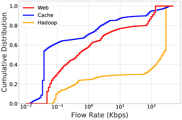
Specifically, [23] investigates the traffic flowing through the network of one of Facebook’s large datacenter, and reports, among other things, the distribution of flow sizes and durations (Figs. 6 & 7 of [23]) for three representative applications: Web (W), Cache read and replacement (C), and Hadoop (H). We rely on these data to generate sample traffic profiles $(r,b)$ for flows from those three applications as follows:

  1. 1.

    For a given application, we generate flow size+duration tuples by sampling the corresponding distributions assuming they are perfectly positively correlated. In other words, we assume that larger flows last longer.

  2. 2.

    A flow’s token rate $r$ is then obtained by dividing the flow size by its duration. Fig. 4 shows the resulting cumulative distributions of flow rates for all three applications.

  3. 3.

    Generating token bucket sizes $b$ involves an additional step and associated assumption:

    1. (a)

      The smallest flow sizes from Fig. 6 of [23] are assumed representative of a single transmission burst. This yields burst sizes $S_{W}=0.15$Kbytes, $S_{C}=0.4$Kbytes, and $S_{H}=0.3$Kbytes for our three sample applications.

    2. (b)

      As bucket sizes are typically chosen to accommodate consecutive bursts, we leverage the claim in [23] that all three applications are “internally bursty” with Cache significantly burstier than Hadoop, and Web in between, to randomly select bucket sizes in $[0,20S_{C}],[0,10S_{W}]$ and $[0,2S_{H}]$, respectively. We note that these values yield relatively small buckets, and, therefore, maximum burst sizes.

Refer to caption
Figure 4: CDF of flow rates for Web, Cache, & Hadoop applications from [23] assuming correlated flow durations and sizes.

The resulting profiles have relatively low rates and burstiness, at least when it comes to individual flows, with Hadoop’s profile typical of bandwidth hungry applications, and Web and Cache representative of more interactive applications. This maps to the types of services that [23] mentions as relying on those three applications, i.e., Web search, user data query, and offline analysis (e.g., data mining). As a result, we assign deadlines to each application that broadly reflect those services, with three deadline classes set to $10$ms, $50$ms, and $200$ms for Web, Cache, and Hadoop respectively.

In evaluating performance, we consider four “traffic mixes” that differ in their relative proportion of flows from each application. Specifically, the corresponding four scenarios sample our W, C, H applications in the proportions: 1:1:1, 3:9:1, 9:3:1, and 9:9:1, respectively. For each scenario, we randomly sample $100$ flow profiles in those proportions. The $100$ flows are then grouped according to their deadline class, which yields a set of three aggregates to schedule on the shared link according to their deadlines. This procedure is repeated $1000$ times, and the relative link bandwidth requirements across schedulers and reprofiling options are given in Table III.

TABLE III: Bandwidth savings & benefits of reprofiling.
Application-derived flow profiles.
Comparisons Scenario Mean Std. Dev. $95\%$ Conf.
$\stackrel{{\scriptstyle R^{*}\mbox{ vs. }\widetilde{R}^{*}_{R}}}{{\left(\frac{\widetilde{R}^{*}_{R}-R^{*}}{\widetilde{R}^{*}_{R}}\right)}}$ 1:1:1 $0.0\%$ $0.0\%$ $[0\%,0\%]$
3:9:1 $0.0\%$ $0.0\%$ $[0\%,0\%]$
9:3:1 $0.0\%$ $0.0\%$ $[0\%,0\%]$
9:9:1 $0.0\%$ $0.0\%$ $[0\%,0\%]$
$\stackrel{{\scriptstyle R^{*}\mbox{ vs. }\widehat{R}^{*}_{R}}}{{\left(\frac{\widehat{R}^{*}_{R}-R^{*}}{\widehat{R}^{*}_{R}}\right)}}$ 1:1:1 $41.82\%$ $17.04\%$ $[40.76\%,42.88\%]$
3:9:1 $72.36\%$ $3.43\%$ $[72.15\%,72.58\%]$
9:3:1 $56.84\%$ $8.43\%$ $[56.32\%,57.37\%]$
9:9:1 $69.70\%$ $4.10\%$ $[69.45\%,69.96\%]$
$\stackrel{{\scriptstyle\,}}{{\widetilde{R}^{*}_{R}\mbox{ vs. }\widehat{R}^{*}_{R}}}$ See above
$\stackrel{{\scriptstyle\widetilde{R}^{*}_{R}\mbox{ vs. }\widetilde{R}^{*}}}{{\left(\frac{\widetilde{R}^{*}-\widetilde{R}^{*}_{R}}{\widetilde{R}^{*}}\right)}}$ 1:1:1 $0.01\%$ $0.22\%$ $[0.00\%,0.03\%]$
3:9:1 $1.74\%$ $0.73\%$ $[1.70\%,1.79\%]$
9:3:1 $1.02\%$ $2.34\%$ $[0.87\%,1.16\%]$
9:9:1 $4.06\%$ $1.19\%$ $[3.98\%,4.13\%]$
$\stackrel{{\scriptstyle\widehat{R}^{*}_{R}\mbox{ vs. }\widehat{R}^{*}}}{{\left(\frac{\widehat{R}^{*}-\widehat{R}^{*}_{R}}{\widehat{R}^{*}}\right)}}$ 1:1:1 $22.74\%$ $9.17\%$ $[22.17\%,23.31\%]$
3:9:1 $21.61\%$ $8.48\%$ $[21.09\%,22.14\%]$
9:3:1 $14.93\%$ $8.93\%$ $[14.37\%,15.48\%]$
9:9:1 $19.55\%$ $8.62\%$ $[19.02\%,20.08\%]$

The first conclusion from Table III is that static priority with reprofiling performs just as well as edf for all four scenarios (top four rows). This is not surprising. The large gaps between the deadlines of the three classes of applications ensure that once high-priority bursts are cleared, the residual bandwidth is sufficient to transmit lower priority bursts before their deadline. As with synthetic profiles, reprofiling is instrumental in realizing this outcome, even if the wide gaps between deadlines together with the limited burstiness of the applications produce a smaller gain ($\widetilde{R}^{*}_{R}$ vs. $\widetilde{R}^{*}$).

The benefits of reprofiling are again more apparent with fifo, even if it significantly under-performs both edf and static priority. The lack of discrimination across flows that fifo suffers from is exacerbated by the large gaps between deadlines, and compensating for it calls for an average of about $50\%$ more bandwidth across all four scenarios. However, without reprofiling this bandwidth increase ($\widehat{R}^{*}_{R}$ vs. $\widehat{R}^{*}$) is around $20\%$ larger. This again demonstrates the extent to which reprofiling can help simpler schedulers.

VI-C Summary Discussion

Several common themes emerge between the evaluations of Sections VI-B1 and VI-B2. The first is that reprofiling can help a static priority scheduler perform nearly as well as an edf scheduler. Second, while its inability to discriminate between flows puts fifo at a clear disadvantage, reprofiling is again capable of partially mitigating its handicap. Finally, while with static priority the benefits of reprofiling are realized by reprofiling high-priority flows to limit their impact on low-priority ones, the opposite holds for fifo.

The differences between the results of Sections VI-B1 and VI-B2 also revealed a number of intuitive findings brought about by the differences in deadline spreads in the two scenarios. In particular, the large gaps between deadlines present in Section VI-B2 make it easier for a static priority scheduler to perform nearly as well as an edf scheduler. This holds with and without reprofiling, even if reprofiling remains useful. Conversely, more closely packed deadlines offer additional opportunities for reprofiling to be useful, as closer deadlines amplify the need for fine tuning of a flow’s profile relative to its deadline and impact on other flows.

VII Related Works

The question of meeting deadlines for a set of rate-limited flows is one that has received much attention in the scheduling literature. It is not our intent to provide an exhaustive review of those works. Instead, we limit ourselves to highlighting works whose results are closest to ours or that offered early insight into the problem, including the benefits of adjusting flows’ profiles (reprofiling) that is one of the foci of this paper.

Packet-level shaping and scheduling

Scheduling flows with deterministic traffic profiles was investigated in [18] that considered both buffer and delay requirements. In particular, the paper established999A similar result was reported in [24]. the optimality of the edf policy in terms of maximizing the schedulable region. This is the “dual” of the bandwidth minimization problem investigated in this paper, and the result parallels that of Proposition 2. Static priority and fifo schedulers were, however, not investigated, and neither was the impact of reprofiling flows.

The aspect of minimizing the resources required to meet the latency targets of token bucket-controlled flows was explored in [25]. The paper relied on service curves with high and low rates and sought to identify the earliest possible time for switching to the lower rate. The focus was, however, on minimizing resources required by each flow individually rather than in aggregate, as in this paper. In addition, the potential impact of reprofiling flows was not addressed.

Shaping bulk data transfers

Minimizing bandwidth (cost) through reprofiling (reshaping) flows has been investigated for bulk data transfers where transfer completion times rather than packet-level deadlines are the targets[26, 27, 28, 29, 30, 31]. The problem stems from non-linear bandwidth costs, e.g., based on the $95^{th}$ percentile, so that judiciously adjusting (shaping) the transmission rates of bulk transfers can yield significant savings. Rate shaping is, however, at a time-granularity of minutes rather than at the packet-level. The optimization frameworks of those papers are, therefore, not applicable to our problem. Their solutions, can, however, complement ours by leveraging the fluctuations in link utilization inherent in delivering hard, packet-level delay bounds, as we do.

Deterministic networking

The deterministic traffic profiles and delay bounds of the TSN and DetNet standards have also given rise to related investigations as documented in recent surveys [32, 33]. In particular, the optimization framework that underlies many of those studies have connections to the problem we address. However, like most prior similar works, traffic profiles are assumed fixed and the impact of reprofiling is not considered.

Datacenter solutions

The emergence of traffic profiles and latency targets in datacenter networks motivated [34]. It targets a multi-hop network, but calls on topological properties of typical datacenter networks to collapse its model to a single hop, thereby aligning with the scope of this paper. Similarities extend to considering a static priority scheduler, but traffic profiles differ. Rather than a token bucket, [34] relies on the notion of network “epochs” to bound packet bursts. Delay bounds are then expressed as a function of the network fan-in and a “throughput factor” that reflects the number of transmission opportunities sources can have per network epoch. Also absent from the paper are exploring bandwidth minimization and the potential benefits of reprofiling flows.

Reprofiling investigations

Meeting packet-level latency constraints with a static priority scheduler while minimizing costs through reprofiling of flows is the focus of WorkloadCompactor [15]. The reprofiling decisions of [15] are, however, focused on selecting token bucket parameters from among a family of feasible regulators101010Regulators above the r-b curve using the terminology of [15]. that do not introduce additional delay. In contrast, our reprofiling allows for an added delay that the scheduler must then compensate for. Exploring when and how this trade-off is of benefit is our main contribution and what makes this work complementary to the approach from WorkloadCompactor.

Specifically, WorkloadCompactor considers traffic/workload traces for which it seeks to first identify feasible token bucket parameter pairs $\langle r,b\rangle$ that result in zero access delay for those traces. WorkloadCompactor’s main contribution is in realizing that multiple such $\langle r,b\rangle$ pairs are possible (the $r$-$b$ curve of [15]), and that “jointly optimizing the choice of $\langle r,b\rangle$ rate limit parameters for each workload to better compact workloads onto servers” can reduce the required server capacity. This is where the contribution of WorkloadCompactor ends, and where that of this paper actually starts.

More precisely, once the optimization of WorkloadCompactor completes, the set of $\langle r,b\rangle$ pairs it produces can be used, together with the associated target latency bounds, as inputs to Proposition 8. Proposition 8 explores, for a static priority scheduler, how to best reprofile token bucket-controlled flows to meet their deadlines with the least bandwidth. This reprofiling is beyond that suggested by WorkloadCompactor111111Again [15] focuses on regulators that ensure zero access delay for a given trace, while we investigate how a non-zero access delay can be of benefit., and explores how trading-off access delay to further smooth flows can yield additional benefits. In other words, the approach proposed in the paper complements that of WorkloadCompactor, in that it can be applied to any set of token bucket profiles produced by WorkloadCompactor, and modify them to yield further reductions in system resources (bandwidth or server capacity) while still meeting latency targets.

We also note that, because WorkloadCompactor considers the problem of selecting token bucket parameters for traffic traces (to ensure zero access delay), it addresses an aspect that this paper does not consider since we assume that token bucket profiles are given. This is yet another aspect in which the two papers are complementary.

Early works

Finally, we note that exploring the trade-off between making traffic smoother and end-to-end performance is not unique to packet networks. It is present in the early “fluctuation smoothing” scheduling policies of [35] that sought to reduce processing time in manufacturing plants, and more recently in the reshaping of parallel I/O requests to improve the scalability of database systems [36].

VIII Conclusion and Future Work

The paper investigated the question of minimizing the bandwidth needed to guarantee worst case latencies to a set of token bucket-controlled flows sharing a single link. The investigation was carried for schedulers of different complexity.

The paper first characterized the minimum required bandwidth independent of schedulers, and showed that an edf scheduler could realize all flows’ deadlines under such bandwidth. Motivated by the need for lower complexity solutions, the paper then explored simpler static priority and fifo schedulers. It derived the minimum required bandwidth for both, but more interestingly established how to optimally reprofile flows to reduce the bandwidth needed while still meeting all deadlines. The relative benefits of such an approach were illustrated numerically for a number of different flow combinations, which showed how reprofiling can enable simpler schedulers to perform nearly as well a more complex ones across a range of configurations.

The obvious direction in which to extend the paper is to a multi-hop setting. In [16], we build on the results of Proposition 1 and provide initial results for the multi-hop case under the assumption that (service curve) edf schedulers are available at each hop. Extending the investigation to static priority and fifo schedulers is under way.

Another aspect of interest with static priority schedulers is relaxing the assumption that flows with different deadlines map to distinct priority classes, and allow multiple deadlines to be assigned to the same class. Not only does it enhance scalability, but it can also improve performance121212See Appendix E for the simple case of a two-flow configuration.. Last but not least, extensions to statistical rather than deterministic delay guarantees are also of practical relevance.

References

  • [1] M. Ashjaei, L. L. Bello, M. Daneshtalab, G. Patti, S. Saponara, and S. Mubeen, “Time-sensitive networking in automotive embedded systems: State of the art and research opportunities,” Journal of Systems Architecture, vol. 117, p. 102137, 2021. [Online]. Available: https://www.sciencedirect.com/science/article/pii/S1383762121001028
  • [2] Avionics Full Duplex Switched Ethernet (AFDX) Network, Airlines Electronic Engineering Committee, Aircraft Data Network Part 7, ARINC Specification 664, Aeronautical Radio, Annapolis, MD, USA, 2002.
  • [3] C. Zunino, A. Valenzano, R. Obermaisser, and S. Petersen, “Factory communications at the dawn of the fourth industrial revolution,” Computer Standards & Interfaces, vol. 71, p. 103433, 2020. [Online]. Available: https://www.sciencedirect.com/science/article/pii/S0920548919300868
  • [4] T. Docquier, Y.-Q. Song, V. Chevrier, L. Pontnau, and A. Ahmed-Nacer, “Performance evaluation methodologies for smart grid substation communication networks: A survey,” Computer Communications, vol. 198, pp. 228–246, 2023. [Online]. Available: https://www.sciencedirect.com/science/article/pii/S0140366422004285
  • [5] (2022) AWS global network. [Online]. Available: https://aws.amazon.com/about-aws/global-infrastructure/global_network/
  • [6] (2022) Google cloud networking overview. [Online]. Available: https://cloud.google.com/blog/topics/developers-practitioners/google-cloud-networking-overview
  • [7] (2021, January) Microsoft global network. [Online]. Available: https://docs.microsoft.com/en-us/azure/networking/microsoft-global-network
  • [8] J. Farkas, L. L. Bello, and C. Gunther, “Time-sensitive networking standards,” IEEE Communications Standards Magazine, vol. 2, no. 2, pp. 20–21, June 2018.
  • [9] G. Parsons, “The rise of time-sensitive networking (TSN) in automobiles, industrial automation, and aviation,” In Compliance - Electronic Design, Testing & Standards, January 2022, https://incompliancemag.com/article/the-rise-of-time-sensitive-networking-tsn-in-automobiles-industrial-automation-and-aviation/.
  • [10] Y. Seol, D. Hyeon, J. Min, M. Kim, and J. Paek, “Timely survey of time-sensitive networking: Past and future directions,” IEEE Access, vol. 9, pp. 142 506–142 527, 2021.
  • [11] N. Finn, P. Thubert, B. Varga, and J. Farkas, “Deterministic Networking Architecture,” RFC 8655, October 2019. [Online]. Available: https://www.rfc-editor.org/info/rfc8655
  • [12] C. Jones, J. Wilkes, N. Murphy, and C. Smith, Site Reliability Engineering: How Google Runs Production Systems, B. Beyer, C. Jones, J. Petoff, and N. Murphy, Eds.   O’Reilly Media, 2016, accessible at https://sre.google/sre-book/service-level-objectives/.
  • [13] (2022) Enterprises are willing to pay for an SLA with guaranteed latency, says new 5G MEC report. [Online]. Available: https://www.vanillaplus.com/2022/06/08/70101-enterprises-are-willing-to-pay-for-an-sla-with-guaranteed-latency-says-new-5g-mec-report/
  • [14] J.-Y. Le Boudec, “A theory of traffic regulators for deterministic networks with application to interleaved regulators,” IEEE/ACM Transactions on Networking, vol. 26, no. 6, p. 2721–2733, December 2018. [Online]. Available: https://doi.org/10.1109/TNET.2018.2875191
  • [15] T. Zhu, M. A. Kozuch, and M. Harchol-Balter, WorkloadCompactor: Reducing Datacenter Cost While Providing Tail Latency SLO Guarantees.   Santa Clara, CA: Association for Computing Machinery, September 2017, p. 598–610. [Online]. Available: https://doi.org/10.1145/3127479.3132245
  • [16] J. Qiu, J. Song, R. Guérin, and H. Sariowan, “On the benefits of traffic “reprofiling.” the multiple hops case – Part I,” 2023, under submission.
  • [17] J.-Y. Le Boudec and P. Thiran, Network Calculus: A Theory of Deterministic Queuing Systems for the Internet.   Springer, 2001.
  • [18] L. Georgiadis, R. Guerin, and A. Parekh, “Optimal multiplexing on a single link: delay and buffer requirements,” IEEE Transactions on Information Theory, vol. 43, no. 5, pp. 1518–1535, September 1997.
  • [19] A. K. Parekh and R. G. Gallager, “A generalized processor sharing approach to flow control in integrated services networks: the single-node case,” IEEE/ACM Transactions on Networking, vol. 1, no. 3, pp. 344–357, June 1993.
  • [20] A. Sivaraman, S. Subramanian, M. Alizadeh, S. Chole, S.-T. Chuang, A. Agrawal, H. Balakrishnan, T. Edsall, S. Katti, and N. McKeown, “Programmable packet scheduling at line rate,” in Proc. ACM SIGCOMM, Florianopolis, Brazil, August 2016.
  • [21] A. Saeed, Y. Zhao, N. Dukkipati, M. Ammar, E. Zegura, K. Harras, and A. Vahdat, “Eiffel: Efficient and flexible software packet scheduling,” in Proc. USENIX NSDI, Boston, MA, 2019.
  • [22] N. K. Sharma, C. Zhao, M. Liu, P. G. Kannan, C. Kim, A. Krishnamurthy, and A. Sivaraman, “Programmable calendar queues for high-speed packet scheduling,” in Proc. USENIX NSDI, Santa Clara, CA, February 2020.
  • [23] A. Roy, H. Zeng, J. Bagga, G. Porter, and A. C. Snoeren, “Inside the social network’s (datacenter) network,” in Proc. ACM SIGCOMM, London, United Kingdom, August 2015. [Online]. Available: https://doi.org/10.1145/2785956.2787472
  • [24] J. Liebeherr, D. E. Wrege, and D. Ferrari, “Exact admission control for networks with a bounded delay service,” IEEE/ACM Transactions on Networking, vol. 4, no. 6, pp. 885–901, 1996.
  • [25] J. B. Schmitt, “On the allocation of network service curves for bandwidth/delay-decoupled scheduling disciplines,” in Proc. IEEE GLOBECOM, vol. 2, Taipei, Taiwan, November 2002.
  • [26] T. Nandagopal and K. P. Puttaswamy, “Lowering inter-datacenter bandwidth costs via bulk data scheduling,” in Proc. IEEE/ACM International Symposium on Cluster, Cloud and Grid Computing, Ottawa, ON, Canada, May 2012.
  • [27] H. Zhang, K. Chen, W. Bai, D. Han, C. Tian, H. Wang, H. Guan, and M. Zhang, “Guaranteeing deadlines for inter-datacenter transfers,” in Proc. European Conference on Computer Systems (EuroSys), Bordeaux, France, 2015. [Online]. Available: https://doi.org/10.1145/2741948.2741957
  • [28] V. Jalaparti, I. Bliznets, S. Kandula, B. Lucier, and I. Menache, “Dynamic pricing and traffic engineering for timely inter-datacenter transfers,” in Proc. ACM SIGCOMM, Florianopolis, Brazil, August 2016. [Online]. Available: https://doi.org/10.1145/2934872.2934893
  • [29] W. Li, X. Zhou, K. Li, H. Qi, and D. Guo, “TrafficShaper: Shaping inter-datacenter traffic to reduce the transmission cost,” IEEE/ACM Transactions on Networking, vol. 26, no. 3, pp. 1193–1206, June 2018.
  • [30] Z. Yang, Y. Cui, X. Wang, Y. Liu, M. Li, S. Xiao, and C. Li, “Cost-efficient scheduling of bulk transfers in inter-datacenter WANs,” IEEE/ACM Transactions on Networking, vol. 27, no. 5, pp. 1973–1986, 2019.
  • [31] R. Singh, S. Agarwal, M. Calder, and P. Bahl, “Cost-effective cloud edge traffic engineering with cascara,” in Proc. USENIX NSDI, virtual, 2021. [Online]. Available: https://www.usenix.org/conference/nsdi21/presentation/singh
  • [32] T. Stüber, L. Osswald, S. Lindner, and M. Menth, “A survey of scheduling in time-sensitive networking (TSN),” 2022. [Online]. Available: https://arxiv.org/abs/2211.10954
  • [33] J. Walrand, “A concise tutorial on traffic shaping and scheduling in time-sensitive networks,” IEEE Communications Surveys & Tutorials, pp. 1–1, May 2023.
  • [34] M. P. Grosvenor, M. Schwarzkopf, I. Gog, R. N. M. Watson, A. W. Moore, S. Hand, and J. Crowcroft, “Queues Don’t matter when you can JUMP them!” in Proc. USENIX NSDI, Oakland, CA, May 2015. [Online]. Available: https://www.usenix.org/conference/nsdi15/technical-sessions/presentation/grosvenor
  • [35] S. Lu, D. Ramaswamy, and P. Kumar, “Efficient scheduling policies to reduce mean and variance of cycle-time in semiconductor manufacturing plants,” IEEE Transactions on Semiconductor Manufacturing, vol. 7, no. 3, pp. 374–388, 1994.
  • [36] N. Li, H. Jiang, H. Che, Z. Wang, and M. Q. Nguyen, “Improving scalability of database systems by reshaping user parallel I/O,” in Proc. EuroSys, Rennes, France, April 2022. [Online]. Available: https://doi.org/10.1145/3492321.3519570

Appendix A Summary of Notation Used in the Paper

Notation Definition
$n$ number of flows inside the network
$b_{i}$ token bucket size of flow $i$
$\bm{b}$ vector of token bucket sizes across $n$ flows: $(b_{1},b_{2},\ldots,b_{n})$
$b^{\prime}_{i}$ reprofiled token bucket size of flow $i$
$\bm{b}^{\prime}$ vector for all reprofiled token bucket sizes across $n$ flows: $(b^{\prime}_{1},b^{\prime}_{2},\ldots,b^{\prime}_{n})$
$b^{\prime*}_{i}$ optimal bucket size of flow $i$’s reprofiler under static priority
$\bm{b}^{\prime*}$ vector for all optimal reprofiled token bucket sizes across $n$ flows: $(b^{\prime*}_{1},b^{\prime*}_{2},\ldots,b^{\prime*}_{n})$ under static priority
$\widehat{b}^{\prime*}_{i}$ optimal bucket size of flow $i$’s reprofiler under fifo
$\widehat{\bm{b}}^{\prime*}$ vector for all optimal reprofiled token bucket sizes across $n$ flows: $(\hat{b}^{\prime*}_{1},\hat{b}^{\prime*}_{2},\ldots,\hat{b}^{\prime*}_{n})$ under fifo
$B^{\prime}_{i}$ cumulative reprofiled token bucket size for flows with a priority no smaller than $i$, i.e., $\sum_{j=i}^{n}b^{\prime}_{j}$
$\widehat{B}_{i}$ cumulative token bucket burst size for flows $1$ to $i$, i.e., $\sum_{j=1}^{i}b_{j}$
$\widehat{B}^{\prime}_{i}$ cumulative reprofiled token bucket size for flows from $1$ to $i$, i.e., $\sum_{j=1}^{i}b^{\prime}_{j}$
$d_{i}$ end-to-end deadline for flow $i$
$\bm{d}$ vector of end-to-end deadlines for $n$ flows: $(d_{1},d_{2},\ldots,d_{n})$
$D^{*}_{i}$ worst-case end-to-end delay for flow $i$ under priority+reprofiling
$\widehat{D}^{*}_{i}$ worst-case end-to-end delay for flow $i$ under fifo+reprofiling
$r_{i}$ token bucket rate of flow $i$
$\bm{r}$ vector for all token bucket rates across $n$ flows: $(r_{1},r_{2},\ldots,r_{n})$
$(r_{i},b_{i})$ traffic profile of flow $i$
$R_{i}$ cumulative token bucket rates for flows with a priority no smaller than $i$, i.e., $\sum_{j=i}^{n}r_{j}$
$R$ shared link bandwidth
$R^{*}$ optimal minimum required bandwidth
$\widetilde{R}^{*}$ minimum required link bandwidth in the absence of reprofiling under static priority
$\widetilde{R}^{*}_{R}$ minimum required link bandwidth with reprofiling under static priority
$\widehat{R}^{*}$ minimum required link bandwidth in the absence of reprofiling under fifo
$\widehat{R}^{*}_{R}$ minimum required link bandwidth with reprofiling under fifo
$t$ time
$H_{i}$ $b_{i}-d_{i}r_{i}$
$\Pi_{i}(R)$ $\frac{r_{i}+R-R_{i+1}}{R-R_{i+1}}$
$V_{i}(R)$ $d_{i}(R-R_{i+1}-b_{i})$
$\mathbb{S}_{1}(R)$ ${V_{1}(R)}$
$\mathbb{S}_{i}(r)$ $\mathbb{S}_{i-1}(R)\bigcup{V_{i}(R)}\bigcup\left\{\frac{s-H_{i}}{\Pi_{i}(R)}|s\in\mathbb{S}_{i-1}(R)\right\}$
$\mathbb{Z}_{i}$ the set of integers from $1$ to $i$, i.e., $\left\{1\leq i\leq j|j\in\mathbb{Z}\right\}$
$X_{F}(R)$ $\max_{P_{1},P_{2}\subseteq\mathbb{Z}_{n},P_{2}\neq\mathbb{Z}_{n},P_{1}\bigcap P_{2}=\emptyset}\frac{\sum_{i\in P_{1}}\frac{RH_{i}}{R+r_{i}}+\sum_{i\in P_{2}}\left(b_{i}-\frac{r_{i}d_{i}R}{R_{1}}\right)}{1-\sum_{i\in P_{1}}\frac{r_{i}}{R+r_{i}}-\sum_{i\in P_{2}}\frac{r_{i}}{R_{1}}}$
$Y_{F}(R)$ $\min_{1\leq i\leq n-1}\left\{\widehat{B}_{n},Rd_{n},\min_{P_{1},P_{2}\subseteq\mathbb{Z}_{i},P_{1}\bigcap P_{2}=\emptyset,P_{1}\bigcup P_{2}\neq\emptyset}\left\{\frac{\widehat{B}_{i}-\sum_{j\in P_{1}}\frac{RH_{j}}{R+r_{j}}-\sum_{j\in P_{2}}\left(b_{j}-\frac{r_{j}d_{j}R}{R_{1}}\right)}{\sum_{j\in P_{1}}\frac{r_{j}}{R+r_{j}}+\sum_{j\in P_{2}}\frac{r_{j}}{R_{1}}}\right\}\right\}$
$T_{i}(\widehat{B}^{\prime}_{n},R)$ $\max\left\{0,\frac{R}{R+r_{i}}\left(H_{i}+\frac{r_{i}}{R}\widehat{B}^{\prime}_{n}\right),b_{i}+\frac{r_{i}(\widehat{B}^{\prime}_{n}-Rd_{i})}{R_{1}}\right\}$
$\Gamma_{sc}$ a service curve assignment that gives each flow $i$ a service curve of $SC_{i}(t)$
OPT_❏ general optimization where ❏=S,F for static priority and fifo
OPT_R❏ optimization with reprofiling where ❏=S,F for static priority and fifo

Appendix B Proofs for Dynamic Priority Scheduler

B-A Proof for Proposition 1

For the reader’s convenience, we restate Proposition 1.

PROPOSITION 1. Consider a link shared by $n$ token bucket controlled flows, where flow $i,1\leq i\leq n$, has a traffic profile $(r_{i},b_{i})$ and a deadline $d_{i}$, with $d_{1}>d_{2}>...>d_{n}$ and $d_{1}<\infty$. Consider a service-curve assignment $\Gamma_{sc}$ that allocates flow $i$ a service curve of

SCi(t)={0 when t<di,bi+ri(tdi)otherwise.SC_{i}(t)=\left\{\begin{aligned} &0&\text{ when }t<d_{i},\\ &b_{i}+r_{i}(t-d_{i})&\text{otherwise}.\end{aligned}\right. (1)

Then

  1. 1.

    For any flow $i,1\leq i\leq n$, $SC_{i}(t)$ ensures a worst-case end-to-end delay no larger than $d_{i}$.

  2. 2.

    Realizing $\Gamma_{sc}$ requires a link bandwidth of at least

    $$R^{*}=\max_{1\leq h\leq n}\left\{\sum_{i=1}^{n}r_{i},\frac{\sum_{i=h}^{n}b_{i}+r_{i}(d_{h}-d_{i})}{d_{h}}\right\}.$$ (2)
  3. 3.

    Any scheduling mechanism capable of meeting all the flows’ deadlines requires a bandwidth of at least $R^{*}$.

Proof.

We first show that under $\Gamma_{sc}$ each flow meets its deadline, and then show that a bandwidth of $R^{*}$ is enough to accommodate all the service curves defined in $\Gamma_{sc}$. Next, we show that no mechanism exists than can meet the deadlines with a bandwidth strictly smaller than $R^{*}$.

  • For any flow $1\leq i\leq n$, its token bucket constrained arrival curve is of the form

    $$AC_{i}(t)=\left\{\begin{aligned} &0&\text{ when }t=0\\ &b_{i}+r_{i}t&\text{ otherwise}.\end{aligned}\right.$$

    Combining it with flow $i$’s service curve $SC_{i}(t)$, the worst-case end-to-end delay for flow $i$ is of the form131313See THEOREM 1.4.2 in [17], page 23.,

    $$D^{*}_{i}=\sup_{t\geq 0}\inf_{\tau\geq 0}\left\{AC_{i}(t)\leq SC_{i}(t+\tau)\right\}=d_{i}.$$
  • To accommodate all the service curves in $\Gamma_{sc}$, the system needs a bandwidth $R$ such that $Rt\geq\sum_{i=1}^{n}SC_{i}(t)$ for all $t>0$, i.e.,

    $$R\geq\sup_{t>0}\frac{\sum_{i=1}^{n}SC_{i}(t)}{t}.$$ (16)

    Towards establishing that the minimum link bandwidth $R^{*}=\sup_{t>0}\frac{\sum_{i=1}^{n}SC_{i}(t)}{t}$ is captured by Eq. (2), we first introduce another proposition:

    Proposition 12.

    Assume that $PL(t)$ is a wide-sense increasing, piecewise linear, and right continuous function defined by a finite set of $k$ linear segments:

    $$pl_{i}(t)=c_{i}+s_{i}t,\ t\in[t_{i},t_{i+1}),\ 1\leq i\leq k$$

    where $s_{i}\geq 0$ and $c_{i}$ are the slopes and intercepts of segment $pl_{i}(t)$ respectively, and $t_{i}<t_{i+1},\,\forall i,1\leq i\leq k,$ with $t_{1}=0$ and $t_{k+1}=\infty$. Furthermore, $PL(0)=0$ so that $c_{1}=0$.

    Then, to compute $\sup_{t>0}\frac{PL(t)}{t}$, it is sufficient to consider values of $\frac{PL(t)}{t}$ at the following times $t$:

    1. 1.

      $t\rightarrow t_{k+1}=\infty$

    2. 2.

      interval boundaries $t_{i},\ 2\leq i\leq k,$ when one of the following conditions is met:

      1. (a)

        $PL(t)$ is continuous and the slope of $PL(t)$ decreases, i.e., $s_{i-1}>s_{i}$.

      2. (b)

        $PL(t)$ is discontinuous.

    Proof.

    We readily know that to find $\sup_{t>0}\frac{PL(t)}{t}$, it is sufficient to consider interval boundaries $t_{i}$s, since $\frac{pl_{i}(t)}{t}=\frac{c_{i}}{t}+s_{i}$, $\frac{PL(t)}{t}$ is a decreasing (increasing) function of $t$ within any interval $[t_{i},t_{i+1})$ when $c_{i}\geq 0$ $(c_{i}<0)$.

    Consider first an intermediate boundary $t_{i},2\leq i\leq k$, we first argue that if $PL(t)$ is continuous, then $\sup_{t>0}\frac{PL(t)}{t}$ cannot be achieved at any boundary $t_{i}$ for which $s_{i-1}<s_{i}$, i.e., a boundary where the slope of $PL(t)$ increases. Towards establishing the result, consider the following two cases:

    1. 1.

      $c_{i}<0$. In this case, irrespective of $s_{i}$, $\frac{PL(t)}{t}$ is increasing in $[t_{i},t_{i+1})$ and $\sup_{t\in[t_{i},t_{i+1})}\frac{PL(t)}{t}=\frac{PL(t_{i+1}^{-})}{t_{i+1}^{-}}$, so that $\sup_{t>0}\frac{PL(t)}{t}$ cannot be achieved at $t_{i}$.

    2. 2.

      $c_{i}\geq 0$. Since we have assumed that $PL(t)$ is continuous, we have that $pl_{i-1}(t_{i})=c_{i-1}+s_{i-1}t_{i}=pl_{i}(t_{i})=c_{i}+s_{i}t_{i}$. This implies $c_{i-1}=c_{i}+(s_{i}-s_{i-1})t_{i}>c_{i}\geq 0$ since $s_{i}>s_{i-1}$. Since both $c_{i}$ and $c_{i-1}$ are non-negative, $\frac{PL(t)}{t}$ is a decreasing function throughout $[t_{i-1},t_{i+1})$. Hence, $\sup_{t>0}\frac{PL(t)}{t}$ cannot be realized at $t_{i}$.

    Turning next to the case where $PL(t)$ is discontinuous at some $t_{i}$, then $\lim_{t\rightarrow t_{i}^{-}}\frac{PL(t)}{t}<\lim_{t\rightarrow t_{i}^{+}}\frac{PL(t)}{t}$ since $PL(t)$ is wide-sense increasing. Since $PL(t)$ is right continuous, $\frac{PL(t_{i})}{t_{i}}=\lim_{t\rightarrow t_{i}^{+}}\frac{PL(t)}{t}$, which implies it is sufficient to consider $t_{i}$ for computing the supremum.

    Finally, we consider the two extreme boundaries $t_{1}=0$ and $t_{k+1}=\infty$. For $t_{1}=0$, since $c_{1}=0$, we have $\frac{PL(t)}{t}=s_{1},\forall\,t\in[t_{1}=0,t_{2}).$ Since $t_{2}$ is one of the intermediate boundaries covered by the first part of our proof, we do not need to consider $t_{1}$ when computing the supremum of $\frac{PL(t)}{t}$ For $t_{k+1}=\infty$, $\lim_{t\rightarrow\infty}\frac{PL(t)}{t}=s_{k}$.

    Combining the fact that $\sup_{t>0}\frac{PL(t)}{t}$ can only be realized at an interval boundary with the above establishes that it is realized at either an interval boundary $t_{i}$ where $PL(t)$ is continuous and experiencing a slope decrease, i.e., $s_{i-1}>s_{i}$, or at an interval boundary where $PL(t)$ is discontinuous, or at $t_{k+1}$, i.e., $t\rightarrow\infty$. ∎

    Returning to the proof of Proposition 1, the aggregate service curve $\sum_{i=1}^{n}SC_{i}(t)$ is a wide-sense increasing, piecewise linear function since each $SC_{i}(t)$ is, by definition, wide-sense increasing and piecewise linear. From Proposition 12 we know that the supremum of $\frac{\sum_{i=1}^{n}SC_{i}(t)}{t}$ is either $\lim_{t\rightarrow\infty}\frac{\sum_{i=1}^{n}SC_{i}(t)}{t}=\sum_{i=1}^{n}r_{i}$ or is achieved at a boundary value $d_{k}\in\left\{d_{1},d_{2},\ldots,d_{n}\right\}$. Combining this with the expressions for the individual service curves $SC_{i}(t),i=1,\ldots,n,$ gives

    $$R\geq\max_{1\leq h\leq n}\left\{\sum_{i=1}^{n}r_{i},\ \frac{\sum_{i=h}^{n}b_{i}+r_{i}(d_{h}-d_{i})}{d_{h}}\right\}=R^{*}.$$

    Thus, $R^{*}$ is sufficient to accommodates all service curves in the service curves assignment $\Gamma_{sc}$.

  • Next, we show that $R^{*}$ is a lower bound for the minimum required bandwidth. Note that $R^{*}\geq\sum_{i=1}^{n}r_{i}$, so that if the deadlines can be met with $R^{*}=\sum_{i=1}^{n}r_{i}$ no improvement is feasible. Below we consider the case when $R^{*}>\sum_{i=1}^{n}r_{i}$, i.e., there exists $1\leq\hat{h}\leq n$, such that $R^{*}=\frac{\sum_{i=\hat{h}}^{n}b_{i}+r_{i}(d_{\hat{h}}-d_{i})}{d_{\hat{h}}}>\sum_{i=1}^{n}r_{i}$

    Suppose there exists a mechanism achieving a minimum required bandwidth $R^{\prime}<R^{*}$. Next we construct an arrival pattern consistent with each flow’s token bucket arrival constraints, such that $R^{\prime}$ cannot satisfy all flows’ deadlines.

    Consider the arrival pattern such that for all $1\leq i\leq n$, flow $i$ sends $b_{i}$ at $t=0$ (where the system restarts the clock), and then constantly sends at a rate of $r_{i}$. By time $d_{\hat{h}}$, to satisfy the deadlines of all flows $i$ with $d_{i}\leq d_{\hat{h}}$, i.e., $i\geq\hat{h}$, the link must have transmitted at least $b_{i}+r_{i}(d_{\hat{h}}-d_{i})$ amount of data for each such flow. Consequently, by $d_{\hat{h}}$ the link should have cumulatively transmitted at least $\sum_{i=\hat{h}}^{n}b_{i}+r_{i}(d_{\hat{h}}-d_{i})$. As $\sum_{i=\hat{h}}^{n}b_{i}+r_{i}(d_{\hat{h}}-d_{i})=d_{\hat{h}}R^{*}>d_{\hat{h}}R^{\prime}$, a bandwidth of $R^{\prime}$ must violate some flows’ deadlines.

B-B Proof for Proposition 2

PROPOSITION 2. Consider a link shared by $n$ token bucket controlled flows, where flow $i,1\leq i\leq n$, has traffic profile $(r_{i},b_{i})$ and deadline $d_{i}$, with $d_{1}>d_{2}>...>d_{n}$ and $d_{1}<\infty$. The earliest deadline first (EDF) scheduler realizes $\Gamma_{sc}$ under a link bandwidth of $R^{*}$.

Proof.

We first show that EDF satisfies $\Gamma_{sc}$, and then shows that EDF requires a minimum required bandwidth of $R^{*}$.

We show that EDF satisfies $\Gamma_{sc}$ by contradiction. Suppose EDF cannot achieve $\Gamma_{sc}$. Then there exists $\hat{t}\geq d_{i}$ and $1\leq i\leq n$, such that $\widehat{SC}_{i}(\hat{t})<SC_{i}(\hat{t})$, where $\widehat{SC}_{i}$ is the service curve that EDF assigns to flow $i$. To satisfy flow $i$’s deadline, at $\hat{t}-d_{i}$ EDF should yield a virtual delay no large than $d_{i}$, i.e.,

$$\inf_{\tau\geq 0}\left\{b_{i}+r_{i}(\hat{t}-d_{i})\leq\widehat{SC}_{i}(\hat{t}-d_{i}+\tau)\right\}\leq d_{i},$$

which then gives $\widehat{SC}_{i}(\hat{t}-d_{i}+d_{i})\geq b_{i}+r_{i}(\hat{t}-d_{i})$. As $b_{i}+r_{i}(\hat{t}-d_{i})=SC_{i}(\hat{t})$, this contradicts the assumption that $\widehat{SC}_{i}(\hat{t})<SC_{i}(\hat{t})$.

Next, we show that EDF requires a minimum bandwidth of $R^{*}$. Suppose flow $i$’s data sent at $t$ has a deadline of $(t+d_{i})$. We show that EDF satisfies all flows’ deadlines with a bandwidth of $R^{*}=\max_{1\leq h\leq n}\left\{\sum_{i=1}^{n}r_{i},\frac{\sum_{i=h}^{n}b_{i}+r_{i}(d_{h}-d_{i})}{d_{h}}\right\}$. Based on the utilization of the shared link, we consider two cases separately, where in both cases we prove the result by contradiction. Specifically, suppose that under EDF, $R^{*}$ cannot satisfy all flows’ latency requirements. Then there exists $1\leq\hat{h}\leq n$ and $\hat{t}\geq 0$, such that EDF processes at least one bit sent by flow $\hat{h}$ at time $\hat{t}$ after time $(\hat{t}+d_{\hat{h}})$. We consider first the case where the shared link uses up all its bandwidth during the period $[0,\hat{t}+d_{\hat{h}}]$ to transmit data with absolute deadlines no larger than $(\hat{t}+d_{\hat{h}})$, and then consider the case where there exists $t_{0}\in[0,\hat{t}+d_{\hat{h}}]$, such that at $t_{0}$ the shared link is not busy with data whose absolute deadline is no larger than $(\hat{t}+d_{\hat{h}})$. Showing that $R^{*}$ is enough for EDF to meet all flows’ deadlines, establishes the result.

  1. 1.

    Consider the case where for all $t\in[0,\hat{t}+d_{\hat{h}}]$ the shared link uses up all its bandwidth to send bits with an absolute deadline no larger than $(\hat{t}+d_{\hat{t}})$. Then by $(\hat{t}+d_{\hat{h}})$ the shared link cumulatively has processed $R^{*}(\hat{t}+d_{\hat{h}})$ amount of data that all have deadlines no larger than $(\hat{t}+d_{\hat{t}})$. From the fact that EDF violates an absolute deadline of $(\hat{t}+d_{\hat{h}})$, we know that there exists an arrival pattern consistent with the token bucket constraints, such that cumulatively flows send more than $R^{*}(\hat{t}+d_{\hat{h}})$ amount of data with absolute deadlines no larger than $(\hat{t}+d_{\hat{h}})$. From the token bucket constraints, we know that by $(\hat{t}+d_{\hat{h}})$, flows can send at most $\sum_{i=1}^{n}\left[b_{i}+r_{i}(\hat{t}+d_{\hat{h}}-d_{i})\right]\bf{I}_{\hat{t}+d_{\hat{h}}-d_{i}\geq 0}$ amount of data whose absolute deadline is at most $(\hat{t}+d_{\hat{h}})$. Therefore, we have $R^{*}(\hat{t}+d_{\hat{h}})<\sum_{i=1}^{n}\left[b_{i}+r_{i}(\hat{t}+d_{\hat{h}}-d_{i})\right]\bf{I}_{\hat{t}+d_{\hat{h}}-d_{i}\geq 0}$. Define $d_{0}=\infty$. There exists $1\leq\hat{n}\leq n$ such that $\hat{t}+d_{\hat{h}}\in[d_{\hat{n}},d_{\hat{n}-1})$ so that

    $$R^{*}<\frac{\sum_{i=1}^{n}\left[b_{i}+r_{i}(\hat{t}+d_{\hat{h}}-d_{i})\right]\bf{I}_{\hat{t}+d_{\hat{h}}-d_{i}\geq 0}}{\hat{t}+d_{\hat{h}}}=\sum_{i=\hat{n}}^{n}\left(r_{i}+\frac{b_{i}-r_{i}d_{i}}{\hat{t}+d_{\hat{h}}}\right):=R^{\prime}.$$

    If $\sum_{i=\hat{n}}^{n}b_{i}-r_{i}d_{i}\leq$ 00, we have $R^{*}<R^{\prime}\leq\sum_{i=1}^{n}r_{i}$, which contradicts to $R^{*}>\sum_{i=1}^{n}r_{i}$. Hence we consider only $\sum_{i=\hat{n}}^{n}b_{i}-r_{i}d_{i}>0$, where $R^{\prime}$ decreases with $(\hat{t}+d_{\hat{h}})$. Define $\hat{R}(u)=\sum_{i=\hat{n}}^{n}\left(r_{i}+\frac{b_{i}-r_{i}d_{i}}{u}\right)$. We then have

    $$R^{*}<R^{\prime}\leq\hat{R}(d_{\hat{n}})=\frac{\sum_{i=\hat{n}}^{n}\left[b_{i}+r_{i}(d_{\hat{n}}-d_{i})\right]}{d_{\hat{n}}},$$

    which contradicts to the definition of $R^{*}$.

  2. 2.

    Otherwise, the shared link uses less than all its bandwidth at $t_{0}\in[0,\hat{t}+d_{\hat{h}}]$, and uses up all its bandwidth for all $t\in(t_{0},\hat{t}+d_{\hat{h}}]$ to send bits with an absolute deadline no larger than $(\hat{t}+d_{\hat{t}})$. Then during $(t_{0},\hat{t}+d_{\hat{h}}]$ the shared link processes $R^{*}(\hat{t}+d_{\hat{h}}-t_{0})$ amount of data with absolute deadlines no larger than $(\hat{t}+d_{\hat{h}})$, and flows send strictly more than $R^{*}(\hat{t}+d_{\hat{h}}-t_{0})$ amount of data with absolute deadlines no larger than $(\hat{t}+d_{\hat{h}})$. From the token bucket constraints, we know that during $(t_{0},\hat{t}+d_{\hat{h}}]$ flows can send at most $\sum_{i=1}^{n}\left[b_{i}+r_{i}(\hat{t}+d_{\hat{h}}-t_{0}-d_{i})\right]\bf{I}_{\hat{t}+d_{\hat{h}}-t_{0}-d_{i}\geq 0}$ amount of data whose absolute deadlines are no larger than $(\hat{t}+d_{\hat{h}})$. Thus we have $R^{*}<\frac{\sum_{i=1}^{n}\left[b_{i}+r_{i}(\hat{t}+d_{\hat{h}}-t_{0}-d_{i})\right]\bf{I}_{\hat{t}+d_{\hat{h}}-t_{0}-d_{i}\geq 0}}{d_{\hat{h}}+\hat{t}-t_{0}}$, which, as before, contradicts the definition of $R^{*}$.

B-C Proof for Proposition 3

PROPOSITION 3. Consider a link shared by $n$ token bucket controlled flows, where flow $i,1\leq i\leq n$, has traffic profile $(r_{i},b_{i})$ and deadline $d_{i}$, with $d_{1}>d_{2}>...>d_{n}$ and $d_{1}<\infty$. Reprofiling flows will not decrease the minimum bandwidth required to meet the flows’ deadlines.

Proof.

We show that adding a reprofiler to any of the flow does not decrease the optimal minimum required bandwidth.

Suppose we apply a reprofiler $b^{\prime}_{i}$ to flow $i$, where $1\leq i\leq n$ and $b^{\prime}_{i}\geq b_{i}-d_{i}r_{i}$. Then flow $i$ incurs a reshaping delay of $\frac{b_{i}-b^{\prime}_{i}}{r_{i}}$. This then leaves a maximum in-network delay of $d_{i}-\frac{b_{i}-b^{\prime}_{i}}{r_{i}}$, which is greater than 00 since $b^{\prime}_{i}\geq b_{i}-d_{i}r_{i}$. Hence, to meet its deadline flow $i$ requires a service curve of at least

$$SC^{\prime}_{i}(t)=\left\{\begin{aligned} &0,&\text{when }t<d_{i}-\frac{b_{i}-b^{\prime}_{i}}{r_{i}}\\ &b^{\prime}_{i}+r_{i}\left(t-d_{i}+\frac{b_{i}-b^{\prime}_{i}}{r_{i}}\right)=b_{i}+r_{i}(t-d_{i}),&\text{otherwise}\end{aligned}\right.$$

which is greater than $SC_{i}(t)=\left\{\begin{aligned} &0,&\text{when }t<d_{i}\\ &b_{i}+r_{i}(t-d_{i}),&\text{otherwise}\end{aligned}\right.$. Consequently, according to Proposition 1 the system needs a bandwidth of at least

$$R=\max\left\{\sum_{i=1}^{n}r_{i},\sup_{t\geq 0}\frac{\sum_{j\neq i}SC_{j}(t)+SC^{\prime}_{i}(t)}{t}\right\}\geq\max\left\{\sum_{i=1}^{n}r_{i},\sup_{t\geq 0}\frac{\sum_{1\leq j\leq n}SC_{j}(t)}{t}\right\}=R^{*}_{sc},$$ (17)

to meet each flow’s deadline. ∎

Appendix C Proofs for Static Priority Scheduler

C-A Proof for Proposition 4

We actually prove Proposition 4 under the more general packet-based model. By assuming that all packets have a length of 00, the packet-based model defaults to the fluid model.

PROPOSITION 4. Consider a link shared by $n$ token bucket controlled flows, where flow $i,1\leq i\leq n$, has traffic profile $(r_{i},b_{i})$ and deadline $d_{i}$, with $d_{1}>d_{2}>...>d_{n}$ and $d_{1}<\infty$. Under a static-priority scheduler, there exists an assignment of flows to priorities that minimizes link bandwidth while meeting all flows deadlines such that flow $i$ is assigned a priority strictly greater than that of flow $j$ only if $d_{i}<d_{j}$.

Proof.

For a mechanism $\Gamma$, denote flows with priority $h$ under $\Gamma$ as $G_{h}(\Gamma)$. Define $d^{(max)}_{h}(\Gamma)=\max_{i\in G_{h}(\Gamma)}d_{i}$ and $d^{(min)}_{h}(\Gamma)=\min_{i\in G_{h}(\Gamma)}d_{i}$. Assume priority class $h+1$ has a higher priority than priority class $h$. Then we will prove the proposition by induction on the number $k$ of priority classes. Our induction hypothesis $S(k)$ is expressed in the following statement:

$S(k)$: For link shared by any number of flows, there exists an optimal $k$-priority mechanism $\Gamma_{k}$ such that $\forall s<l\leq k$, $d^{(max)}_{l}(\Gamma_{k})<d^{(min)}_{s}(\Gamma_{k})$.

  • Base case: consider the case when $k=2$. We show that for any mechanism $\Gamma_{2}$, if $d^{(min)}_{1}(\Gamma_{2})<d^{(max)}_{2}(\Gamma_{2})$, then there exists a 2-priority mechanism $\Gamma^{\prime}_{2}$ such that $d^{(min)}_{1}(\Gamma^{\prime}_{2})>d^{(max)}_{2}(\Gamma^{\prime}_{2})$ and $R^{*}(\Gamma^{\prime}_{2})\leq R^{*}(\Gamma_{2})$.

    For mechanism $\Gamma_{2}$, denote $l_{1}^{(max)}(\Gamma_{2})$ to be the maximum packet size for flows in $G_{1}(\Gamma_{2})$. To satisfy each flow’s deadline, it requires a bandwidth $R$ such that

    $$\left\{\quad\begin{aligned} &\frac{\sum_{i\in G_{2}(\Gamma_{2})}b_{i}+l_{1}^{(max)}(\Gamma_{2})}{R}\leq d^{(min)}_{2}(\Gamma_{2}),\\ &\frac{\sum_{i}b_{i}}{R-\sum_{i\in G_{2}(\Gamma_{2})}r_{i}}\leq d^{(min)}_{1}(\Gamma_{2}),\\ &\sum_{i=1}^{n}r_{i}\leq R,\end{aligned}\right.$$ (18)

    which gives

    $$R^{*}(\Gamma_{2})=\max\left\{\ \sum_{i=1}^{n}r_{i},\frac{\sum_{i\in G_{2}(\Gamma_{2})}b_{i}+l_{1}^{(max)}(\Gamma_{2})}{d^{(min)}_{2}(\Gamma_{2})},\frac{\sum_{i}b_{i}}{d^{(min)}_{1}(\Gamma_{2})}+\sum_{i\in G_{2}(\Gamma_{2})}r_{i}\ \right\}.$$

    Define $G^{\prime}_{1}(\Gamma_{2})=\{i\in G_{2}(\Gamma_{2})\ |\ d_{i}>d^{(max)}_{1}(\Gamma_{2})\}$ and $G^{\prime}_{2}(\Gamma_{2})=G_{2}(\Gamma_{2})-G^{\prime}_{1}(\Gamma_{2})$. Consider the mechanism $\Gamma^{\prime}_{2}$ such that $G_{2}(\Gamma^{\prime}_{2})=G^{\prime}_{2}(\Gamma_{2})$, and $G_{1}(\Gamma^{\prime}_{2})=G^{\prime}_{1}(\Gamma_{2})\cup G_{1}(\Gamma_{2})$. Note that $d^{(min)}_{1}(\Gamma^{\prime}_{2})>d^{(max)}_{2}(\Gamma^{\prime}_{2})$, and note also that $d^{(min)}_{i}(\Gamma^{\prime}_{2})=d^{(min)}_{i}(\Gamma_{2}),i=1,2$. Similar as Eq. (18), we have

    $R^{*}(\Gamma^{\prime}_{2})=\max\left\{\ \sum_{i=1}^{n}r_{i},\frac{\sum_{i\in G_{2}(\Gamma^{\prime}_{2})}b_{i}+l_{1}^{(max)}(\Gamma^{\prime}_{2})}{d^{(min)}_{2}(\Gamma_{2})},\frac{\sum_{i}b_{i}}{d^{(min)}_{1}(\Gamma_{2})}+\sum_{i\in G_{2}(\Gamma_{2})-G^{\prime}_{1}(\Gamma_{2})}r_{i}\ \right\}$

    Note that $\frac{\sum_{i}b_{i}}{d^{(min)}_{1}(\Gamma_{2})}+\sum_{i\in G_{2}(\Gamma_{2})}r_{i}\geq\frac{\sum_{i}b_{i}}{d^{(min)}_{1}(\Gamma_{2})}+\sum_{i\in G_{2}(\Gamma_{2})-G^{\prime}_{1}(\Gamma_{2})}r_{i}$. Next we show $\sum_{i\in G_{2}(\Gamma_{2})}b_{i}+l_{1}^{(max)}(\Gamma_{2})\geq\sum_{i\in G_{2}(\Gamma^{\prime}_{2})}b_{i}+l_{1}^{(max)}(\Gamma^{\prime}_{2})$, from which we then have $R^{*}(\Gamma_{2})\geq R^{*}(\Gamma^{\prime}_{2})$, and therefore $S(2)$. Since $G_{1}(\Gamma_{2})\varsubsetneqq G_{1}(\Gamma^{\prime}_{2})$, it has $l_{1}^{(max)}(\Gamma^{\prime}_{2})\geq l_{1}^{(max)}(\Gamma_{2})$.

    • When $l_{1}^{(max)}(\Gamma^{\prime}_{2})=l_{1}^{(max)}(\Gamma_{2})$, from $G_{2}(\Gamma^{\prime}_{2})\varsubsetneqq G_{2}(\Gamma_{2})$ we have $\sum_{i\in G_{2}(\Gamma_{2})}b_{i}\geq\sum_{i\in G_{2}(\Gamma^{\prime}_{2})}b_{i}$, and therefore have $\sum_{i\in G_{2}(\Gamma_{2})}b_{i}+l_{1}^{(max)}(\Gamma_{2})\geq\sum_{i\in G_{2}(\Gamma^{\prime}_{2})}b_{i}+l_{1}^{(max)}(\Gamma^{\prime}_{2})$.

    • When $l_{1}^{(max)}(\Gamma^{\prime}_{2})>l_{1}^{(max)}(\Gamma_{2})$, i.e., there exists a flow $\hat{i}\in G^{\prime}_{1}(\Gamma_{2})$ such that $l_{\hat{i}}>l_{1}^{(max)}(\Gamma_{2})$. From $b_{\hat{i}}\geq l_{\hat{i}}$ and $G_{2}(\Gamma^{\prime}_{2})\subseteq G_{2}(\Gamma_{2})-\hat{i}$, we have

      $\displaystyle\sum_{i\in G_{2}(\Gamma_{2})}b_{i}+l_{1}^{(max)}(\Gamma_{2})=$ $\displaystyle\sum_{i\in G_{2}(\Gamma_{2})-\hat{i}}b_{i}+b_{\hat{i}}+l_{1}^{(max)}(\Gamma_{2})\geq\sum_{i\in G_{2}(\Gamma^{\prime}_{2})}b_{i}+l_{\hat{i}}+l_{1}^{(max)}(\Gamma_{2})$
      $\displaystyle>$ $\displaystyle\sum_{i\in G_{2}(\Gamma^{\prime}_{2})}b_{i}+l_{1}^{(max)}(\Gamma^{\prime}_{2})$
  • Induction Step: Let $k\geq 2$ and suppose $S(k)$ holds. Next, we show that $S(k+1)$ holds.

    Consider any (k+1)-priority mechanism $\Gamma_{k+1}$. For $1\leq h\leq(1+k)$, denote $l_{h}^{(max)}(\Gamma_{k+1})$ to be the maximum packet size for all flows with priority strictly smaller than $h$, and define $l_{h}^{(max)}(\Gamma_{k+1})$ to be 00 if no flow has a priority strictly smaller than $h$. Define $B_{h}^{(k)}(\Gamma_{k+1})=\sum_{j=h}^{k}\sum_{i\in G_{j}(\Gamma_{k+1})}b_{i}$, i.e., the sum of bucket sizes for flows with priority $h\leq j\leq k$, and $R_{h}^{(k)}(\Gamma_{k+1})=\sum_{j=h}^{k}\sum_{i\in G_{j}(\Gamma_{k+1})}r_{i}$, i.e., the sum of rates for flows with priority in $h\leq j\leq k$. Then to satisfy each flow’s deadline $\Gamma_{k+1}$ requires a bandwidth $R$ satisfying

    $\displaystyle\left\{\begin{array}[]{ll}&\frac{B_{h}^{(k+1)}(\Gamma_{k+1})+l_{h}^{(max)}(\Gamma_{k+1})}{R-R_{h+1}^{(k+1)}(\Gamma_{k+1})}\leq d^{(min)}_{h}(\Gamma_{k+1}),\quad\forall h\in[1,k+1];\\ \\ &\sum_{i=1}^{n}r_{i}\leq R;\end{array}\right.$ (19)

    which gives a minimum required bandwidth of

    $$R^{*}(\Gamma_{k+1})=\max_{1\leq h\leq k+1}\left\{\sum_{i=1}^{n}r_{i},\ \frac{B_{h}^{(k+1)}(\Gamma_{k+1})+l_{h}^{(max)}(\Gamma_{k+1})}{d^{(min)}_{h}(\Gamma_{k+1})}+R_{h+1}^{(k+1)}(\Gamma_{k+1})\right\}.$$ (20)

    Afterwards, we first show that there exists a $(k+1)$-priority mechanism $\Gamma^{\prime}_{k+1}$ satisfying


    • Condition 1: $G_{k+1}(\Gamma^{\prime}_{k+1})=\{i\ |\ d_{n}\leq d_{i}<d_{\hat{n}}\}\text{ where }1\leq\hat{n}\leq n$, and $R^{*}(\Gamma^{\prime}_{k+1})\leq R^{*}(\Gamma_{k+1})$, where $G_{k+1}(\Gamma^{\prime}_{k+1})=\emptyset$ if $\hat{n}=n$.

    After that, under a slight abuse of notation, we show that for any $\Gamma_{k+1}$ satisfying Condition 1, there exists a $(k+1)$-priority mechanism $\Gamma^{\prime}_{k+1}$ satisfying


    • Condition 2: $R^{*}(\Gamma^{\prime}_{k+1})\leq R^{*}(\Gamma_{k+1})$, and $d^{(max)}_{i}(\Gamma^{\prime}_{k+1})<d^{(min)}_{j}(\Gamma^{\prime}_{k+1})$ for all $j<i\leq k+1$.

    Combining them gives $S(k+1)$.

    1. 1.

      We first show the existence of a mechanism $\Gamma^{\prime}_{k+1}$ satisfying condition 1. If $\Gamma_{k+1}$ satisfies Condition 1, then $\Gamma_{k+1}=\Gamma^{\prime}_{k+1}$. Otherwise, for all $1\leq\hat{n}<n$, $G_{k+1}(\Gamma_{k+1})\neq\{i\ |\ d_{n}\leq d_{i}<d_{\hat{n}}\}$. Define $\hat{i}=\max\{1\leq i\leq n\ |\ i\notin G_{k+1}(\Gamma_{k+1})\}$ and suppose $\hat{i}\in G_{\hat{h}}(\Gamma_{k+1})$. Further define $G^{\prime}_{k+1}=\{i\in G_{k+1}(\Gamma_{k+1})\ |\ d_{i}<d^{(min)}_{\hat{h}}(\Gamma_{k+1})\}$ and $G^{\prime}_{\hat{h}}=G_{k+1}(\Gamma_{k+1})-G^{\prime}_{k+1}$.

      Consider the mechanism $\Gamma^{\prime}_{k+1}$ such that 1) $G_{k+1}(\Gamma^{\prime}_{k+1})=G^{\prime}_{k+1}$, 2) $G_{\hat{h}}(\Gamma^{\prime}_{k+1})=G^{\prime}_{\hat{h}}+G_{\hat{h}}(\Gamma_{k+1})$, and 3) $G_{i}(\Gamma^{\prime}_{k+1})=G_{i}(\Gamma_{k+1})$, when $1\leq i\leq k$ and $i\neq\hat{h}$. Note that

      • when $h\leq\hat{h}$, $B_{h}^{(k+1)}(\Gamma^{\prime}_{k+1})=B_{h}^{(k+1)}(\Gamma_{k+1})$, $R_{h}^{(k+1)}(\Gamma^{\prime}_{k+1})=R_{h}^{(k+1)}(\Gamma_{k+1})$, and $l_{h}^{(max)}(\Gamma^{\prime}_{k+1})=l_{h}^{(max)}(\Gamma_{k+1})$;

      • when $h>\hat{h}$, $B_{h}^{(k+1)}(\Gamma^{\prime}_{k+1})=B_{h}^{(k+1)}(\Gamma_{k+1})-\sum_{i\in G^{\prime}_{\hat{h}}}b_{i}$, $R_{h}^{(k+1)}(\Gamma^{\prime}_{k+1})=R_{h}^{(k+1)}(\Gamma^{\prime}_{k+1})-\sum_{i\in G^{\prime}_{\hat{h}}}r_{i}$, and $l_{h}^{(max)}(\Gamma^{\prime}_{k+1})=\max\left\{l_{h}^{(max)}(\Gamma_{k+1}),\ \max_{i\in G^{\prime}_{\hat{h}}}l_{i}\right\}$.

      Next we show that $R^{*}(\Gamma^{\prime}_{k+1})\leq R^{*}(\Gamma_{k+1})$. To satisfy each flow’s deadline, $\Gamma^{\prime}_{k+1}$ requires a bandwidth $R$ such that141414When $G_{k+1}(\Gamma^{\prime}_{k+1})=\emptyset$, $\frac{B_{k+1}^{(k+1)}(\Gamma_{k+1})-\sum_{i\in G^{\prime}_{\hat{h}}}b_{i}+l^{(max)}_{k+1}(\Gamma^{\prime}_{k+1})}{R}=\frac{\max_{i}l_{i}}{R}$, which is also no greater than $d_{n}$.

      $$\left\{\quad\begin{aligned} &\sum_{i=1}^{n}r_{i}\leq R,\\ &\frac{B_{k+1}^{(k+1)}(\Gamma_{k+1})-\sum_{i\in G^{\prime}_{\hat{h}}}b_{i}+l^{(max)}_{k+1}(\Gamma^{\prime}_{k+1})}{R}\leq d_{n},\\ &\frac{B_{\hat{h}}^{(k+1)}(\Gamma_{k+1})+l_{\hat{h}}^{(max)}(\Gamma_{k+1})}{R-R_{\hat{h}+1}^{(k+1)}(\Gamma_{k+1})+\sum_{i\in G^{\prime}_{\hat{h}}}r_{i}}\leq d^{(min)}_{\hat{h}}(\Gamma_{k+1})\\ &\frac{B_{h}^{(k+1)}(\Gamma_{k+1})-\sum_{i\in G^{\prime}_{\hat{h}}}b_{i}+l_{h}^{(max)}(\Gamma^{\prime}_{k+1})}{R-R_{h+1}^{(k+1)}(\Gamma_{k+1})+\sum_{i\in G^{\prime}_{\hat{h}}}r_{i}}\leq d^{(min)}_{h}(\Gamma_{k+1}),\text{ when }\hat{h}<h\leq k\\ &\frac{B_{h}^{(k+1)}(\Gamma_{k+1})+l_{h}^{(max)}(\Gamma_{k+1})}{R-R_{h+1}^{(k+1)}(\Gamma_{k+1})}\leq d^{(min)}_{h}(\Gamma_{k+1}),\text{ when }h<\hat{h}\\ \end{aligned}\right.$$

      which gives a minimum required bandwidth $R^{*}(\Gamma^{\prime})$ of

      $$\max\left\{\quad\begin{aligned} &\sum_{i=1}^{n}r_{i},\\ &\frac{B_{k+1}^{(k+1)}(\Gamma_{k+1})-\sum_{i\in G^{\prime}_{\hat{h}}}b_{i}+l^{(max)}_{k+1}(\Gamma^{\prime}_{k+1})}{d_{n}},\\ &\frac{B_{\hat{h}}^{(k+1)}(\Gamma_{k+1})+l_{\hat{h}}^{(max)}(\Gamma_{k+1})}{d^{(min)}_{\hat{h}}(\Gamma_{k+1})}+R_{\hat{h}+1}^{(k+1)}(\Gamma_{k+1})-\sum_{i\in G^{\prime}_{\hat{h}}}r_{i}\\ &\frac{B_{h}^{(k+1)}(\Gamma_{k+1})-\sum_{i\in G^{\prime}_{\hat{h}}}b_{i}+l_{h}^{(max)}(\Gamma^{\prime}_{k+1})}{d^{(min)}_{h}(\Gamma_{k+1})}+R_{h+1}^{(k+1)}(\Gamma_{k+1})-\sum_{i\in G^{\prime}_{\hat{h}}}r_{i},\text{ when }\hat{h}<h\leq k\\ &\frac{B_{h}^{(k+1)}(\Gamma_{k+1})+l_{h}^{(max)}(\Gamma_{k+1})}{d^{(min)}_{h}(\Gamma_{k+1})}+R_{h+1}^{(k+1)}(\Gamma_{k+1}),\text{ when }h<\hat{h}\end{aligned}\right.$$

      Note that if for all $\hat{h}<h\leq k+1$, $l_{h}^{(max)}(\Gamma^{\prime}_{k+1})-\sum_{i\in G^{\prime}_{\hat{h}}}b_{i}\leq l_{h}^{(max)}(\Gamma_{k+1})$, we will then have $R^{*}(\Gamma^{\prime}_{k+1})\leq R^{*}(\Gamma_{k+1})$. In fact, as $\max_{i\in G^{\prime}_{\hat{h}}}l_{i}-\sum_{i\in G^{\prime}_{\hat{h}}}b_{i}\leq 0$ we have

      $\displaystyle l_{h}^{(max)}(\Gamma^{\prime}_{k+1})-\sum_{i\in G^{\prime}_{\hat{h}}}b_{i}$ $\displaystyle=\max\left\{l_{h}^{(max)}(\Gamma_{k+1}),\ \max_{i\in G^{\prime}_{\hat{h}}}l_{i}\right\}-\sum_{i\in G^{\prime}_{\hat{h}}}b_{i}$
      $\displaystyle\leq\max\left\{l_{h}^{(max)}(\Gamma_{k+1})-\sum_{i\in G^{\prime}_{\hat{h}}}b_{i},0\right\}<l_{h}^{(max)}(\Gamma_{k+1}).$

      Thus, we show the existence of a mechanism $\Gamma^{\prime}_{k+1}$ satisfying Condition 1.

    2. 2.

      Next we show that for any $(k+1)$-priority mechanism $\Gamma_{k+1}$ satisfying Condition 1, there exists a $(k+1)$-priority mechanism $\Gamma^{\prime}_{k+1}$ satisfying Condition 2.

      For $\Gamma_{k+1}$, there to exist $1\leq\hat{n}\leq n$ such that $G_{k+1}(\Gamma_{k+1})=\{i\ |\ d_{n}\leq d_{i}<d_{\hat{n}}\ \}$. If $G_{k+1}(\Gamma_{k+1})=\emptyset$, by induction of hypothesis $S(k)$ we have $S(k+1)$. Afterwards we consider the case where $G_{k+1}(\Gamma_{k+1})\neq\emptyset$.

      Consider flows $\tilde{F}=\{(r_{1},b_{1},l_{1},d_{1}),...,(r_{\hat{n}-1},b_{\hat{n}-1},l_{\hat{n}-1},d_{\hat{n}-1}),(r_{\hat{n}},\sum_{i\geq\hat{n}}b_{i},l_{\hat{n}},d_{\hat{n}})\}$. According to $S(k)$, there exists a $k$-priority mechanism $\Gamma^{\prime}_{k}$ for $\tilde{F}$ such that $\forall j<i\leq k$, $\tilde{d}^{(max)}_{i}(\Gamma^{\prime}_{k})<\tilde{d}^{(min)}_{j}(\Gamma^{\prime}_{k})$. $\Gamma_{k}$ gives a minimum required bandwidth of

      $$R^{*}(\Gamma^{\prime}_{k})=\max_{1\leq h\leq k}\left\{\sum_{i=1}^{\hat{n}}r_{i},\ \frac{\tilde{B}_{h}^{(k)}(\Gamma^{\prime}_{k})+l_{h}^{(max)}(\Gamma^{\prime}_{k})}{d^{(min)}_{h}(\Gamma^{\prime}_{k})}+\tilde{R}_{h+1}^{(k)}(\Gamma^{\prime}_{k})\right\}$$

      Consider the $k$-priority mechanism $\Gamma_{k}$, where $G_{h}(\Gamma_{k})=G_{h}(\Gamma_{k+1})$ for all $1\leq h\leq k$. Applying $\Gamma_{k}$ to $\tilde{F}$, we have

      $\displaystyle R^{*}(\Gamma_{k})$ $\displaystyle=\max_{1\leq h\leq k}\left\{\sum_{i=1}^{\hat{n}}r_{i},\frac{\tilde{B}_{h}^{(k)}(\Gamma_{k})+l_{h}^{(max)}(\Gamma_{k})}{d^{(min)}_{h}(\Gamma_{k})}+\tilde{R}_{h+1}^{(k)}(\Gamma_{k})\right\}$
      $\displaystyle=\max_{1\leq h\leq k}\left\{\sum_{i=1}^{\hat{n}}r_{i},\frac{B_{h}^{(k+1)}(\Gamma_{k+1})+l_{h}^{(max)}(\Gamma_{k+1})}{d^{(min)}_{h}(\Gamma_{k+1})}+R_{h+1}^{(k+1)}(\Gamma_{k+1})-\sum_{i=\hat{n}+1}^{n}r_{i}\right\}.$

      From $R^{*}(\Gamma_{k})\geq R^{*}(\Gamma^{\prime}_{k})$, we know that

      $\displaystyle\max_{1\leq h\leq k}\left\{\frac{\tilde{B}_{h}^{(k)}(\Gamma^{\prime}_{k})+l_{h}^{(max)}(\Gamma^{\prime}_{k})}{d^{(min)}_{h}(\Gamma^{\prime}_{k})}+\tilde{R}_{h+1}^{(k)}(\Gamma^{\prime}_{k})\right\}$
      $\displaystyle\qquad\leq\max\left\{\ \sum_{i=1}^{\hat{n}}r_{i},\ \max_{1\leq h\leq k}\left\{\frac{B_{h}^{(k+1)}(\Gamma_{k+1})+l_{h}^{(max)}(\Gamma)}{d^{(min)}_{h}(\Gamma_{k+1})}+R_{h+1}^{(k+1)}(\Gamma_{k+1})-\sum_{i=\hat{n}+1}^{n}r_{i}\right\}\ \right\}$

      which further gives

      $\displaystyle\max_{1\leq h\leq k}\left\{\frac{\tilde{B}_{h}^{(k)}(\Gamma^{\prime}_{k})+l_{h}^{(max)}(\Gamma^{\prime}_{k})}{d^{(min)}_{h}(\Gamma^{\prime}_{k})}+\tilde{R}_{h+1}^{(k)}(\Gamma^{\prime}_{k})+\sum_{i=\hat{n}+1}^{n}r_{i}\right\}$ (21)
      $\displaystyle\qquad\leq\max\left\{\ \sum_{i=1}^{n}r_{i},\max_{1\leq h\leq k}\left\{\frac{B_{h}^{(k+1)}(\Gamma_{k+1})+l_{h}^{(max)}(\Gamma_{k+1})}{d^{(min)}_{h}(\Gamma_{k+1})}+R_{h+1}^{(k+1)}(\Gamma_{k+1})\right\}\ \right\}$

      Now consider the $(k+1)$-priority mechanism $\Gamma^{\prime}_{k+1}$, where $G_{h}(\Gamma^{\prime}_{k+1})=G_{h}(\Gamma^{\prime}_{k})$ for all $1\leq h\leq k$, and $G_{k+1}(\Gamma^{\prime}_{k+1})=G_{k+1}(\Gamma_{k+1})$. By the definition of $G_{k+1}(\Gamma_{k+1})$ and $\Gamma^{\prime}_{k}$, we know that $d^{(max)}_{i}(\Gamma^{\prime}_{k+1})<d^{(min)}_{j}(\Gamma^{\prime}_{k+1}),\forall j<i\leq k+1$. Next we show that $R^{*}(\Gamma^{\prime}_{k+1})\leq R^{*}(\Gamma_{k+1})$.

      Applying $\Gamma^{\prime}_{k+1}$ to flow $F=\{(r_{i},b_{i},l_{i},d_{i})\ |\ 1\leq i\leq n\}$, we have

      $\displaystyle R^{*}(\Gamma^{\prime}_{k+1})=\max_{1\leq h\leq k+1}\left\{\sum_{i=1}^{n}r_{i},\ \frac{B_{h}^{(k+1)}(\Gamma^{\prime}_{k+1})+l_{h}^{(max)}(\Gamma^{\prime}_{k+1})}{d^{(min)}_{h}(\Gamma^{\prime}_{k+1})}+R_{h+1}^{(k+1)}(\Gamma^{\prime}_{k+1})\right\}$
      $\displaystyle\quad=\max_{1\leq h\leq k}\left\{\sum_{i=1}^{n}r_{i},\frac{B_{k+1}^{(k+1)}(\Gamma_{k+1})+l_{k+1}^{(max)}(\Gamma_{k+1})}{d^{(min)}_{k+1}(\Gamma_{k+1})},\frac{B_{h}^{(k+1)}(\Gamma^{\prime}_{k+1})+l_{h}^{(max)}(\Gamma^{\prime}_{k+1})}{d^{(min)}_{h}(\Gamma^{\prime}_{k+1})}+R_{h+1}^{(k+1)}(\Gamma^{\prime}_{k+1})\right\}$
      $\displaystyle\quad=\max_{1\leq h\leq k}\left\{\sum_{i=1}^{n}r_{i},\frac{B_{k+1}^{(k+1)}(\Gamma_{k+1})+l_{k+1}^{(max)}(\Gamma_{k+1})}{d^{(min)}_{k+1}(\Gamma_{k+1})},\frac{\tilde{B}_{h}^{(k)}(\Gamma^{\prime}_{k})+l_{h}^{(max)}(\Gamma^{\prime}_{k})}{d^{(min)}_{h}(\Gamma^{\prime}_{k})}+\tilde{R}_{h+1}^{(k)}(\Gamma^{\prime}_{k})+\sum_{i=\hat{n}+1}^{n}r_{i}\right\}$

      Combining it with Eq. (21), we have

      $\displaystyle R^{*}(\Gamma^{\prime}_{k+1})$ $\displaystyle\leq\max\left\{\begin{array}[]{ll}\sum_{i=1}^{n}r_{i},\\ \\ \frac{B_{k+1}^{(k+1)}(\Gamma_{k+1})+l_{k+1}^{(max)}(\Gamma_{k+1})}{d^{(min)}_{k+1}(\Gamma_{k+1})},\\ \\ \max_{1\leq h\leq k}\left\{\frac{B_{h}^{(k+1)}(\Gamma_{k+1})+l_{h}^{(max)}(\Gamma_{k+1})}{d^{(min)}_{h}(\Gamma_{k+1})}+R_{h+1}^{(k+1)}(\Gamma_{k+1})\right\}\end{array}\right.$
      $\displaystyle=\max\left\{\sum_{i=1}^{n}r_{i},\max_{1\leq h\leq k+1}\left\{\frac{B_{h}^{(k+1)}(\Gamma_{k+1})+l_{h}^{(max)}(\Gamma_{k+1})}{d^{(min)}_{h}(\Gamma_{k+1})}+R_{h+1}^{(k+1)}(\Gamma_{k+1})\right\}\right\}$
      $\displaystyle=R^{*}(\Gamma_{k+1})$

      Hence we show the existence of a mechanism $\Gamma^{\prime}_{k+1}$ satisfying Condition 2.

C-B Proof for Proposition 5

PROPOSITION 5. Consider a link shared by $n$ token bucket controlled flows, where flow $i,1\leq i\leq n$, has traffic profile $(r_{i},b_{i})$. Assume a static priority scheduler that assigns flow $i$ a priority of $i$, where priority $n$ is the highest priority, and reprofiles flow $i$ to $(r_{i},b^{\prime}_{i})$, where $0\leq b^{\prime}_{i}\leq b_{i}$. Given a link bandwidth of $R\geq\sum_{j=1}^{n}r_{j}$, the worst-case delay for flow $i$ is

$$D^{*}_{i}=\max\left\{\frac{b_{i}+B^{\prime}_{i+1}}{R-R_{i+1}},\ \frac{b_{i}-b^{\prime}_{i}}{r_{i}}+\frac{B^{\prime}_{i+1}}{R-R_{i+1}}\right\}.$$ (6)
Proof.

Flow $1\leq i\leq n$ receives a service curve of $SC^{(i)}_{1}=\left\{\begin{aligned} &b^{\prime}_{i}+r_{i}t,\text{ when }t>0\\ &0\qquad\text{otherwise}\end{aligned}\right.$ inside the reprofiler, and a service curve of $SC^{(i)}_{2}(t)=\left[(R-R_{i+1})t-B^{\prime}_{i+1}\right]^{+}$ at the shared link. Overall it receives a service curve of151515See THEOREM 1.4.6 in [17], page 28

$$SC^{(i)}(t)=SC^{(i)}_{1}\otimes SC^{(i)}_{2}=\min\left\{\left[b^{\prime}_{i}+r_{i}\left(t-\frac{B^{\prime}_{i+1}}{R-R_{i+1}}\right)\right]^{+},[(R-R_{i+1})t-B^{\prime}_{i+1}]^{+}\right\}.$$

Hence, we have

$$D^{*}_{i}=\sup_{t\geq 0}\inf_{\tau\geq 0}\left\{b_{i}+r_{i}t\leq SC^{(i)}(t+\tau)\right\}=\max\left\{\frac{b_{i}+B^{\prime}_{i+1}}{R-R_{i+1}},\ \frac{b_{i}-b^{\prime}_{i}}{r_{i}}+\frac{B^{\prime}_{i+1}}{R-R_{i+1}}\right\}.$$

C-C Proofs for Proposition 7 and 8

This section provides the solution for OPT_RSP, from which Propositions 7 and 8 derive. For the reader’s convenience, we restate OPT_RSP. Remember that we define $B^{\prime}_{i}=\sum_{j=i}^{n}b^{\prime}_{j}$ and $R_{i}=\sum_{j=i}^{n}r_{j}$, where $B^{\prime}_{i},R_{i}=0$ when $i>n$.

OPT_RSP $\displaystyle\min_{\bm{b}^{\prime}}R$
s.t $\displaystyle\max\left\{\frac{b_{i}+B^{\prime}_{i+1}}{R-R_{i+1}},\ \frac{b_{i}-b^{\prime}_{i}}{r_{i}}+\frac{B^{\prime}_{i+1}}{R-R_{i+1}}\right\}\leq d_{i},$ $\displaystyle\forall\ 1\leq i\leq n,$
$\displaystyle R_{1}\leq R,\qquad b^{\prime}_{1}\leq b_{1},\qquad 0\leq b^{\prime}_{i}\leq b_{i},$ $\displaystyle\forall\ 2\leq i\leq n.$

Instead of solving OPT_RSP, for technical simplicity we consider OPT_RSP’, whose solution directly gives that for OPT_RSP. Next we first demonstrate the relationship between OPT_RSP and OPT_RSP’ (Lemma 13), and then proceed to solve OPT_RSP’ (Lemma 14). Combining Lemma 13 and 14, we then have Proposition 7 and 8.

Lemma 13.

For $1\leq i\leq n$, define $H_{i}=b_{i}-r_{i}d_{i}$, and $\bm{B^{\prime}}=(B^{\prime}_{1},...,B^{\prime}_{n})$. Consider the following optimization:

OPT_RSP’ $\displaystyle\min_{\bm{B}^{\prime}}R$ (22)
s.t $\displaystyle R_{1}\leq R.$
$\displaystyle B^{\prime}_{2}\leq d_{1}(R-R_{2})-b_{1},$
$\displaystyle B^{\prime}_{i}\in\left[\max\left\{\frac{R-R_{i+1}+r_{i}}{R-R_{i+1}}B^{\prime}_{i+1}+H_{i},\ B^{\prime}_{i+1}\right\},\ B^{\prime}_{i+1}+\frac{b_{i}(R-R_{i})}{R-R_{i+1}}\right],$ $\displaystyle\forall\ 2\leq i\leq n.$

Suppose the optimal solution for OPT_RSP’ is $(R^{*},\bm{B}^{\prime*})$. Then $(R^{*},\bm{b}^{\prime*})$, where

$$\bm{b}^{\prime*}=(b_{1},B^{\prime*}_{2}-B^{\prime*}_{3},....,B^{\prime*}_{n-1}-B^{\prime*}_{n},B^{\prime*}_{n}),$$

is an optimal solution for OPT_RSP.

Proof.

We first show that $\bm{b^{\prime}}^{*}=(b_{1},B^{\prime*}_{2}-B^{\prime*}_{3},....,B^{\prime*}_{n-1}-B^{\prime*}_{n},B^{\prime*}_{n})$ and $R^{*}$ satisfy all the constraints for OPT_RSP, and then show that $(R^{*},\bm{b^{\prime}}^{*})$ is an optimal solution for OPT_RSP.

Substituting $b^{\prime}_{1}=b_{1}$ into $\max\left\{\frac{b_{1}+B^{\prime}_{2}}{R-R_{2}},\ \frac{b_{1}-b^{\prime}_{1}}{r_{1}}+\frac{B^{\prime}_{2}}{R-R_{2}}\right\}\leq d_{1}$ gives $\frac{b_{1}+B^{\prime}_{2}}{R-R_{2}}\leq d_{1}$, which is equivalent to $B^{\prime}_{2}\leq d_{1}(R-R_{2})-b_{1}$. Thus, to show the feasibility of $(R^{*},\bm{b^{\prime}}^{*})$, we only need to show that $(R^{*},\bm{b^{\prime}}^{*})$ satisfies $\max\left\{\frac{b_{i}+B^{\prime*}_{i+1}}{R^{*}-R_{i+1}},\ \frac{b_{i}-b^{\prime*}_{i}}{r_{i}}+\frac{B^{\prime*}_{i+1}}{R^{*}-R_{i+1}}\right\}\leq d_{i}$ and $b^{\prime*}_{i}\in[0,b_{i}]$ for all $2\leq i\leq n$. Below we consider each constraint separately.

  • Basic algebraic manipulation gives that

    $$\max\left\{\frac{b_{i}+B^{\prime*}_{i+1}}{R^{*}-R_{i+1}},\ \frac{b_{i}-b^{\prime*}_{i}}{r_{i}}+\frac{B^{\prime*}_{i+1}}{R^{*}-R_{i+1}}\right\}=\left\{\begin{aligned} &\frac{b_{i}+B^{\prime*}_{i+1}}{R^{*}-R_{i+1}},&\text{ when }b^{\prime*}_{i}\geq\frac{b_{i}(R^{*}-R_{i})}{R^{*}-R_{i+1}},\\ &\frac{b_{i}-b^{\prime*}_{i}}{r_{i}}+\frac{B^{\prime*}_{i+1}}{R^{*}-R_{i+1}},&\text{ otherwise}.\end{aligned}\right.$$ (23)

    From OPT_RSP’ we have $B^{\prime*}_{i}\leq B^{\prime*}_{i+1}+\frac{b_{i}(R^{*}-R_{i})}{R^{*}-R_{i+1}}$, i.e., $b^{\prime*}_{i}=B^{\prime*}_{i}-B^{\prime*}_{i+1}\leq\frac{b_{i}(R^{*}-R_{i})}{R^{*}-R_{i+1}}$, and therefore $\max\left\{\frac{b_{i}+B^{\prime*}_{i+1}}{R^{*}-R_{i+1}},\ \frac{b_{i}-b^{\prime*}_{i}}{r_{i}}+\frac{B^{\prime*}_{i+1}}{R^{*}-R_{i+1}}\right\}=\frac{b_{i}-b^{\prime*}_{i}}{r_{i}}+\frac{B^{\prime*}_{i+1}}{R^{*}-R_{i+1}}$. From OPT_RSP’ we also have $B^{\prime*}_{i}\geq\frac{R^{*}-R_{i+1}+r_{i}}{R^{*}-R_{i+1}}B^{\prime*}_{i+1}+H_{i}$, i.e., $B^{\prime*}_{i}-B^{\prime*}_{i+1}-H_{i}=b^{\prime*}_{i}-b_{i}+r_{i}d_{i}\geq\frac{r_{i}B^{\prime*}_{i+1}}{R-R_{i+1}}$, which is equivalent to $\frac{b_{i}-b^{\prime*}_{i}}{r_{i}}+\frac{B^{\prime*}_{i+1}}{R-R_{i+1}}\leq d_{i}$. Combining them gives $\max\left\{\frac{b_{i}+B^{\prime*}_{i+1}}{R^{*}-R_{i+1}},\ \frac{b_{i}-b^{\prime*}_{i}}{r_{i}}+\frac{B^{\prime*}_{i+1}}{R^{*}-R_{i+1}}\right\}\leq d_{i}$.

  • From OPT_RSP’ we have $B^{\prime*}_{i}\geq B^{\prime*}_{i+1}$, and therefore $b^{\prime*}_{i}=B^{\prime*}_{i}-B^{\prime*}_{i+1}\geq 0$. From OPT_RSP’ we also have $B^{\prime*}_{i}\leq B^{\prime*}_{i+1}+\frac{b_{i}(R^{*}-R_{i})}{R^{*}-R_{i+1}}$, and therefore $b^{\prime*}_{i}\leq\frac{b_{i}(R^{*}-R_{i})}{R^{*}-R_{i+1}}<b_{i}$. Thus, we have $b^{\prime*}_{i}\in[0,b_{i}]$.

Next we show by contradiction that $(R^{*},\bm{b^{\prime}}^{*})$ is optimal for OPT_RSP. Suppose $(\tilde{R},\bm{\tilde{b}^{\prime}})$, where $\tilde{R}<R^{*}$ is an optimal solution for OPT_RSP. Denote $\tilde{B}^{\prime}_{i}=\sum_{j=i}^{n}\tilde{b}^{\prime}_{j}$, and $\bm{\tilde{B}^{\prime}}=(\tilde{B}^{\prime}_{1},...,\tilde{B}^{\prime}_{n})$.

  • If $(\tilde{R},\bm{\tilde{B}^{\prime}})$ satisfies all constraints for OPT_RSP’, then by $(R^{*},\bm{b^{\prime}}^{*})$’s optimality we know that $\tilde{R}\geq R^{*}$, which contradicts to the assumption that $\tilde{R}<R^{*}$.

  • Otherwise, there exists $2\leq i\leq n$ such that $\max\left\{\frac{b_{i}+\tilde{B}^{\prime}_{i+1}}{\tilde{R}-R_{i+1}},\ \frac{b_{i}-\tilde{b}^{\prime}_{i}}{r_{i}}+\frac{\tilde{B}^{\prime}_{i+1}}{\tilde{R}-R_{i+1}}\right\}\leq d_{i}$ and $\tilde{b}^{\prime}_{i}\in[0,b_{i}]$, whereas $\tilde{B}^{\prime}_{i}\notin\left[\max\left\{\frac{\tilde{R}-R_{i+1}+r_{i}}{\tilde{R}-R_{i+1}}\tilde{B}^{\prime}_{i+1}+H_{i},\ \tilde{B}^{\prime}_{i+1}\right\},\ \tilde{B}^{\prime}_{i+1}+\frac{b_{i}(\tilde{R}-R_{i})}{\tilde{R}-R_{i+1}}\right]$.

    • When $\tilde{b}^{\prime}_{i}\leq\frac{b_{i}(\tilde{R}-R_{i})}{\tilde{R}-R_{i+1}}$, from Eq. (23) we have that $\max\left\{\frac{b_{i}+\tilde{B}^{\prime}_{i+1}}{\tilde{R}-R_{i+1}},\ \frac{b_{i}-\tilde{b}^{\prime}_{i}}{r_{i}}+\frac{\tilde{B}^{\prime}_{i+1}}{\tilde{R}-R_{i+1}}\right\}=\frac{b_{i}-\tilde{b}^{\prime}_{i}}{r_{i}}+\frac{\tilde{B}^{\prime}_{i+1}}{\tilde{R}-R_{i+1}}$. Combining $\frac{b_{i}-\tilde{b}^{\prime}_{i}}{r_{i}}+\frac{\tilde{B}^{\prime}_{i+1}}{\tilde{R}-R_{i+1}}\leq d_{i}$ and $\tilde{b}^{\prime}_{i}\in[0,\frac{b_{i}(\tilde{R}-R_{i})}{\tilde{R}-R_{i+1}}]$ with $\tilde{b}^{\prime}_{i}=\tilde{B}^{\prime}_{i}-\tilde{B}^{\prime}_{i-1}$, we have

      $$\tilde{B}^{\prime}_{i}\in\left[\max\left\{\frac{\tilde{R}-R_{i+1}+r_{i}}{\tilde{R}-R_{i+1}}\tilde{B}^{\prime}_{i+1}+H_{i},\ \tilde{B}^{\prime}_{i+1}\right\},\ \tilde{B}^{\prime}_{i+1}+\frac{b_{i}(\tilde{R}-R_{i})}{\tilde{R}-R_{i+1}}\right],$$

      and therefore a contradiction.

    • When $\tilde{b}^{\prime}_{i}>\frac{b_{i}(\tilde{R}-R_{i})}{\tilde{R}-R_{i+1}}$, we show that there exists an optimal solution $(\tilde{R},\bm{\hat{b}^{\prime}})$ for OPT_RSP such that $\hat{b}^{\prime}_{i}\leq\frac{b_{i}(\tilde{R}-R_{i})}{\tilde{R}-R_{i+1}}$. Define $\bm{\hat{b}^{\prime}}$ as 1) $\hat{b}^{\prime}_{i}=\frac{b_{i}(\tilde{R}-R_{i})}{\tilde{R}-R_{i+1}}$, and 2) $\hat{b}^{\prime}_{h}=\tilde{b}^{\prime}_{h}$ when $h\neq i$. Denote $\hat{B}^{\prime}_{h}=\sum_{j=h}^{n}\hat{b}^{\prime}_{j}\leq\tilde{B}^{\prime}_{h}$, and $\bm{\hat{B}^{\prime}}=(\hat{B}^{\prime}_{1},...,\hat{B}^{\prime}_{n})$. Next we show that $(\tilde{R},\bm{\hat{b}^{\prime}})$ satisfies all the constraints in OPT_RSP, and therefore is optimal. Observe first that from $\hat{B}^{\prime}_{2}<\tilde{B}^{\prime}_{2}$, we have $\frac{b_{1}+\hat{B}^{\prime}_{2}}{\tilde{R}-R_{2}}<\frac{b_{1}+\tilde{B}^{\prime}_{2}}{\tilde{R}-R_{2}}\leq d_{1}$. Below we show that for all $2\leq h\leq n$, $\max\left\{\frac{b_{h}+\hat{B}^{\prime}_{h+1}}{\tilde{R}-R_{h+1}},\ \frac{b_{h}-\hat{b}^{\prime}_{h}}{r_{h}}+\frac{\hat{B}^{\prime}_{h+1}}{\tilde{R}-R_{h+1}}\right\}\leq d_{h}$.

      • *

        When $h>i$, by definition $\hat{B}^{\prime}_{h+1}=\tilde{B}^{\prime}_{h+1}$. Thus we have

        $$\max\left\{\frac{b_{h}+\hat{B}^{\prime}_{h+1}}{\tilde{R}-R_{h+1}},\ \frac{b_{h}-\hat{b}^{\prime}_{h}}{r_{h}}+\frac{\hat{B}^{\prime}_{h+1}}{\tilde{R}-R_{h+1}}\right\}=\max\left\{\frac{b_{h}+\tilde{B}^{\prime}_{h+1}}{\tilde{R}-R_{h+1}},\ \frac{b_{h}-\tilde{b}^{\prime}_{h}}{r_{h}}+\frac{\tilde{B}^{\prime}_{h+1}}{\tilde{R}-R_{h+1}}\right\}\leq d_{h}.$$
      • *

        When $h=i$, $\max\left\{\frac{b_{h}+\hat{B}^{\prime}_{h+1}}{\tilde{R}-R_{h+1}},\ \frac{b_{h}-\hat{b}^{\prime}_{h}}{r_{h}}+\frac{\hat{B}^{\prime}_{h+1}}{\tilde{R}-R_{h+1}}\right\}=\frac{b_{h}+\hat{B}^{\prime}_{h+1}}{\tilde{R}-R_{h+1}}$. Combining it with $\hat{B}^{\prime}_{h+1}<\tilde{B}^{\prime}_{h+1}$ and $\max\left\{\frac{b_{h}+\tilde{B}^{\prime}_{h+1}}{\tilde{R}-R_{h+1}},\ \frac{b_{h}-\tilde{b}^{\prime}_{h}}{r_{h}}+\frac{\tilde{B}^{\prime}_{h+1}}{\tilde{R}-R_{h+1}}\right\}=\frac{b_{h}+\tilde{B}^{\prime}_{h+1}}{\tilde{R}-R_{h+1}}\leq d_{h}$ gives the result.

      • *

        When $h<i$, from $\hat{B}^{\prime}_{h+1}<\tilde{B}^{\prime}_{h+1}$ we have $\frac{b_{h}+\hat{B}^{\prime}_{h+1}}{\tilde{R}-R_{h+1}}<\frac{b_{h}+\tilde{B}^{\prime}_{h+1}}{\tilde{R}-R_{h+1}}$ and $\frac{b_{h}-\hat{b}^{\prime}_{h}}{r_{h}}+\frac{\hat{B}^{\prime}_{h+1}}{\tilde{R}-R_{h+1}}<\frac{b_{h}-\tilde{b}^{\prime}_{h}}{r_{h}}+\frac{\tilde{B}^{\prime}_{h+1}}{\tilde{R}-R_{h+1}}$, i.e., $\max\left\{\frac{b_{h}+\hat{B}^{\prime}_{h+1}}{\tilde{R}-R_{h+1}},\ \frac{b_{h}-\hat{b}^{\prime}_{h}}{r_{h}}+\frac{\hat{B}^{\prime}_{h+1}}{\tilde{R}-R_{h+1}}\right\}<\max\left\{\frac{b_{h}+\tilde{B}^{\prime}_{h+1}}{\tilde{R}-R_{h+1}},\ \frac{b_{h}-\tilde{b}^{\prime}_{h}}{r_{h}}+\frac{\tilde{B}^{\prime}_{h+1}}{\tilde{R}-R_{h+1}}\right\}\leq d_{h}.$

      If $(\tilde{R},\bm{\hat{b}^{\prime}})$ satisfies all the constraints for OPT_RSP, it contradicts to the assumption that $\tilde{R}<R^{*}$. Otherwise, from the case for $\tilde{b}^{\prime}_{i}\leq\frac{b_{i}(\tilde{R}-R_{i})}{\tilde{R}-R_{i+1}}$, we know it again to produce a contradiction.

Next, we proceed to solve OPT_RSP’, which when combine with Lemma 13 then gives Propositions 7 and 8. For the reader’s convenience, we restate the Propositions.

PROPOSITION 7. For $1\leq i\leq n$, denote $H_{i}=b_{i}-d_{i}r_{i}$, $\Pi_{i}(R)=\frac{r_{i}+R-R_{i+1}}{R-R_{i+1}}$ and $V_{i}(R)=d_{i}(R-R_{i+1})-b_{i}$. Define $S_{1}(R)=\left\{V_{1}(R)\right\}$, and $S_{i}(R)=S_{i-1}(R)\bigcup\left\{V_{i}(R)\right\}\bigcup\left\{\frac{s-H_{i}}{\Pi_{i}(R)}\ |\ s\in S_{i-1}(R)\right\}$ for $2\leq i\leq n$. Then we have $\tilde{R}^{*}_{R}=\max\left\{R_{1},\inf\{R\ |\ \forall s\in S_{n}(R),s\geq 0\}\right\}$.

PROPOSITION 8. The optimal reprofiling solution $\bm{b}^{\prime*}$ satisfies

$$b^{\prime*}_{i}=\left\{\begin{aligned} &\max\{0,b_{n}-r_{n}d_{n}\},&i=n;\\ &\max\left\{0,\ b_{i}-r_{i}d_{i}+\frac{r_{i}B^{\prime*}_{i+1}}{\tilde{R}^{*}_{R}-R_{i+1}}\right\},&2\leq i\leq n-1.\end{aligned}\right.$$ (7)

Denote $\mathbb{B}_{i}:=\left[\max\left\{\frac{R-R_{i+1}+r_{i}}{R-R_{i+1}}B^{\prime}_{i+1}+H_{i},\ B^{\prime}_{i+1}\right\},\ B^{\prime}_{i+1}+\frac{b_{i}(R-R_{i})}{R-R_{i+1}}\right]$, where the interval overlaps with that in the third constraint of OPT_RSP’. We then show that the system meets each flow’s deadline only if the shared link has a bandwidth no less than $\max\left\{R_{1},\inf\{R\ |\ \forall s\in S_{n}(R),s\geq 0\right\}$, which in turn gives the minimum required bandwidth $R^{*}$. As mentioned before, we achieve this by first solving OPT_RSP’, from which we then get the solution for OPT_RSP based on Lemma 13.

Lemma 14.

Define $s^{(i)}_{1}=\max\left\{\Pi_{i}(R)B^{\prime}_{i+1}+H_{i},\ B^{\prime}_{i+1}\right\}$, $s^{(i)}_{2}=\min\left\{S_{i-1}(R),B^{\prime}_{i+1}+\frac{b_{i}(R-R_{i})}{R-R_{i+1}}\right\}$, and $\mathbb{S}_{i}=\left[s^{(i)}_{1},s^{(i)}_{2}\right]$ for $2\leq i\leq n$, where $\Pi_{i}(R)=\frac{r_{i}+R-R_{i+1}}{R-R_{i+1}}$, $H_{i}=b_{i}-d_{i}r_{i}$, $S_{1}(R)=\left\{V_{1}(R)\right\}$, $V_{i}(R)=d_{i}(R-R_{i+1})-b_{i}$, and $S_{i}(R)=S_{i-1}(R)\bigcup\left\{V_{i}(R)\right\}\bigcup\left\{\frac{s-H_{i}}{\Pi_{i}(R)}\ |\ s\in S_{i-1}(R)\right\}$. Then $R$ and $\bm{b}^{\prime}$ satisfies all the constraints in OPT_RSP’ iff $\mathbb{S}_{n}\neq\emptyset$ and $R\geq R_{1}$, i.e., $R\geq\max\left\{R_{1},\inf\{R\ |\ \forall s\in S_{n}(R),s\geq 0\}\right\}$.

Proof.

We rely on the following statements to show the Lemma:


Statement 1. $\left\{(R,\bm{b}^{\prime})\ |\ B^{\prime}_{i-1}\in\mathbb{S}_{i-1}\right\}\bigcap\left\{(R,\bm{b}^{\prime})\ |\ B^{\prime}_{i}\in\mathbb{B}_{i}\right\}=\left\{(R,\bm{b}^{\prime})\ |\ B^{\prime}_{i}\in\mathbb{S}_{i}\right\}$.

Given Statement 1, we then show that


Statement 2. $\left\{(R,\bm{b}^{\prime})\ |\ B^{\prime}_{2}\leq V_{1}(R),B^{\prime}_{i}\in\mathbb{B}_{i},\forall\ 2\leq i\leq n\right\}=\left\{(R,\bm{b}^{\prime})\ |\ B^{\prime}_{n}\in\mathbb{S}_{n}\right\}.$

Note that $B^{\prime}_{2}\leq V_{1}(R)$ corresponds to the second constraint in OPT_RSP’, while $B^{\prime}_{i}\in\mathbb{B}_{i},\forall\ 2\leq i\leq n$ corresponds to its third constraint. Therefore, from Statement 2 we have that $R$ and $\bm{b}^{\prime}$ satisfies all the constraints in OPT_RSP’ iff $\mathbb{S}_{n}\neq\emptyset$ and $R\geq R_{1}$. Note that $\mathbb{S}_{n}\neq\emptyset$ iff $s^{(n)}_{1}\leq s^{(n)}_{2}$, i.e., $\max\{H_{n},0\}\leq\min\left\{S_{n-1}(R),\frac{b_{n}(R-R_{n})}{R}\right\}$. As $(R-R_{n})\geq 0$, $\max\{H_{n},0\}\leq\frac{b_{n}(R-R_{n})}{R}$ iff $V_{n}(R)\geq 0$, whereas $\max\{H_{n},0\}\leq\min\left\{S_{n-1}(R)\right\}$ iff $s\geq\max\{0,H_{n}\},\forall s\in S_{n-1}(R)$. Since $\Pi_{n}(R)>0$, by the definition of $S_{n}$ we have $\mathbb{S}_{n}\neq\emptyset$ and $R\geq R_{1}$ iff $R\geq\max\left\{R_{1},\inf\{R\ |\ \forall s\in S_{n}(R),s\geq 0\}\right\}$.

Proof for Statement 1.

Note that $\left\{(R,\bm{b}^{\prime})\ |\ B^{\prime}_{i-1}\in\mathbb{S}_{i-1}\right\}=\left\{(R,\bm{b}^{\prime})\ |\ \mathbb{S}_{i-1}\neq\emptyset\right\}$. Below we prove that $\mathbb{S}_{i-1}\neq\emptyset$ iff $B^{\prime}_{i}\leq\min\{S_{i-1}(R)\}$. As $s^{(i)}_{2}=\min\left\{S_{i-1}(R),B^{\prime}_{i+1}+\frac{b_{i}(R-R_{i})}{R-R_{i+1}}\right\}$, combining $B^{\prime}_{i}\leq\min\{S_{i-1}(R)\}$ with $B^{\prime}_{i}\in\mathbb{B}_{i}=\left[s^{(1)}_{i},\ B^{\prime}_{i+1}+\frac{b_{i}(R-R_{i})}{R-R_{i+1}}\right]$ directly gives $B^{\prime}_{i}\in\mathbb{S}_{i}=\left[s^{(i)}_{1},s^{(i)}_{2}\right]$.

From $\mathbb{S}_{i-1}\neq\emptyset\Leftrightarrow s^{(i-1)}_{2}\geq s^{(i-1)}_{1}$, we have

$$\left\{\begin{aligned} &B^{\prime}_{i}\leq s^{(i-1)}_{2}=\min\left\{S_{i-2}(R),B^{\prime}_{i}+\frac{b_{i-1}(R-R_{i-1})}{R-R_{i}}\right\}\Leftrightarrow B^{\prime}_{i}\leq\min\left\{S_{i-2}(R)\right\}\\ &\Pi_{i-1}(R)B^{\prime}_{i}+H_{i-1}\leq s^{(i-1)}_{2}\Leftrightarrow B^{\prime}_{i}\leq\min\{V_{i-1}(R)\}\bigcup\left\{\frac{s-H_{i-1}}{\Pi_{i-1}(R)}\ |\ s\in S_{i-2}(R)\right\}\end{aligned}\right.$$

As $S_{i-1}(R)=S_{i-2}(R)\bigcup\{V_{i-1}(R)\}\bigcup\left\{\frac{s-H_{i-1}}{\Pi_{i-1}(R)}\ |\ s\in S_{i-2}(R)\right\}$, we have $\mathbb{S}_{i-1}\neq\emptyset$ iff $B^{\prime}_{i}\leq\min\{S_{i-1}(R)\}$.

Proof for Statement 2.

We show by induction on the value of $n$.

  • Base case: when $n=2$, basic algebraic manipulation gives that

    $\displaystyle\left\{(R,\bm{b}^{\prime})\ |\ B^{\prime}_{2}\leq V_{1}(R),B^{\prime}_{2}\in\mathbb{B}_{i}\right\}$ $\displaystyle=\left\{(R,\bm{b}^{\prime})\ |\ B^{\prime}_{2}\in\left[s^{(2)}_{1},\min\left\{V_{1}(R),B^{\prime}_{3}+\frac{b_{2}(R-R_{2})}{R-R_{3}}\right\}\right]\right\}$
    $\displaystyle=\left\{(R,\bm{b}^{\prime})\ |\ B^{\prime}_{2}\in\mathbb{S}_{2}\right\}$
  • Induction step: suppose $\left\{(R,\bm{b}^{\prime})\ |\ B^{\prime}_{2}\leq V_{1}(R),B^{\prime}_{i}\in\mathbb{B}_{i},\forall\ 2\leq i\leq k\right\}=\left\{(R,\bm{b}^{\prime})\ |\ B^{\prime}_{k}\in\mathbb{S}_{k}\right\}$. Then we have

    $\displaystyle\left\{(R,\bm{b}^{\prime})\ |\ B^{\prime}_{2}\leq V_{1}(R),B^{\prime}_{i}\in\mathbb{B}_{i},\forall\ 2\leq i\leq k+1\right\}$
    $\displaystyle=$ $\displaystyle\left\{(R,\bm{b}^{\prime})\ |\ B^{\prime}_{2}\leq V_{1}(R),B^{\prime}_{i}\in\mathbb{B}_{i},\forall\ 2\leq i\leq k\right\}\bigcap\left\{(R,\bm{b}^{\prime})\ |\ B^{\prime}_{k+1}\in\mathbb{B}_{k+1}\right\}$
    $\displaystyle=$ $\displaystyle\left\{(R,\bm{b}^{\prime})\ |\ B^{\prime}_{k}\in\mathbb{S}_{k}\right\}\bigcap\left\{(R,\bm{b}^{\prime})\ |\ B^{\prime}_{k+1}\in\mathbb{B}_{k+1}\right\}$
    $\displaystyle=$ $\displaystyle\left\{(R,\bm{b}^{\prime})\ |\ B^{\prime}_{k+1}\in\mathbb{S}_{k+1}\right\}$

    where the last equation comes from Statement $1$.

  • Conclusion: by the principle of induction, we have

    $$\left\{(R,\bm{b}^{\prime})\ |\ B^{\prime}_{2}\leq V_{1}(R),B^{\prime}_{i}\in\mathbb{B}_{i},\forall\ 2\leq i\leq n\right\}=\left\{(R,\bm{b}^{\prime})\ |\ B^{\prime}_{n}\in\mathbb{S}_{n}\right\}.$$

Observe from the proof of Lemma 14 that for all $2\leq i\leq n$, setting $B^{\prime}_{i}=\max\left\{\Pi_{i}(R)B^{\prime}_{i+1}+H_{i},\ B^{\prime}_{i+1}\right\}$ gives $\tilde{R}^{*}_{R}$. Combining it with Lemma 13, we know that $R^{*}$ is the optimal solution for OPT_RSP, and therefore we have Proposition 7. Besides, since $\tilde{R}^{*}_{R}$ can be achieved by setting $b^{\prime}_{i}=\max\left\{\frac{r_{i}B^{\prime}_{i+1}}{R-R_{i+1}}+H_{i},\ 0\right\}$, we then have Proposition 8.

Appendix D Proofs for FIFO Scheduler

D-A Proof for Proposition 9

PROPOSITION 9. Consider a system with $n$ token bucket controlled flows with traffic profiles $(r_{i},b_{i}),1\leq i\leq n$, sharing a fifo link with bandwidth $R\geq R_{1}=\sum_{j=1}^{n}r_{j}$. Assume that the system reprofiles flow $i$ to $(r_{i},b^{\prime}_{i})$. The worst-case delay for flow $i$ is then

$$\widehat{D}^{*}_{i}=\max\left\{\frac{b_{i}-b^{\prime}_{i}}{r_{i}}+\frac{\sum_{j\neq i}b^{\prime}_{j}}{R},\frac{\sum_{j=1}^{n}b^{\prime}_{j}}{R}+\frac{(b_{i}-b^{\prime}_{i})R_{1}}{r_{i}R}\right\}.$$ (8)
Proof.

W.l.o.g we consider the worst-case delay for flow $1$. First we show that there always exists a traffic pattern such that flow $1$’s worst-case delay can be achieved by the last bit inside a burst of size $b_{1}$, and then we characterize the worst-case delay for that $b_{1}^{th}$ bit.

  • Consider the traffic pattern $\bm{T}(t)=\left\{T_{1}(t),...,T_{n}(t)\right\}$ that realizes flow $1$’s worst-case delay, where $T_{i}(t)$ is right continuous and specifies the cumulative amount of data sent by flow $i$ during time $[0,t]$. Suppose the worst-case delay is achieved at $t_{0}$, and at $t_{0}$ flow $1$ sends a burst of $b\leq b_{1}$. As under FIFO the last bit gets a strictly larger delay compared with all the other bits inside the burst, the $b^{th}$ bit sent at $t_{0}$ achieves the worst-case delay.

    If $b=b_{1}$, flow $1$’s worst-case delay is achieved by the $b_{1}^{th}$ bit inside a burst, i.e., $\bm{T}(t)$ is the traffic pattern we want. Afterwards we consider the case $b<b_{1}$.

    First note that $b$ is the maximum amount of data flow $1$ can send at $t_{0}$ without violating its arrival-curve constraint, i.e., there exists $t_{s}\in[0,t_{0})$ such that $T(t_{0})-T(t_{s})=b_{1}+r_{1}(t_{0}-t_{s})$. Otherwise, we can produce a worse delay by increasing $b$ to the maximum value that remains conformant with the arrival-curve constraint. Next we show that if $b<b_{1}$, there exists $T^{\prime}_{1}(t)$ sending a burst of $b_{1}$ at $t_{0}$, such that under $\bm{T}^{\prime}(t)=\left\{T^{\prime}_{1}(t),...,T_{n}(t)\right\}$ the last bit flow $1$ sends at $t_{0}$ also achieves flow $1$’s worst-case delay.

    Define $\hat{t}=\sup\{t\ |\ T_{1}(t_{0})-T(t)\geq b_{1}\}$. As $b<b_{1}$, $\hat{t}\in(t_{s},t_{0})$. Note that $T_{1}(t_{0})-T_{1}(\hat{t})\leq b_{1}$ as $T_{1}(t)$ is right continuous. Define

    $$T^{\prime}_{1}(t)=\left\{\begin{aligned} &T_{1}(t),&\text{ when }t<\hat{t}\\ &T_{1}(t_{0})-b_{1},&\text{ when }\hat{t}\leq t<t_{0}\\ &T_{1}(t_{0}),&\text{ otherwise }\end{aligned}\right.$$

    which sends a burst of $b_{1}$ at $t_{0}$. Note that $T^{\prime}_{1}(t)$ satisfies flow $1$’s arrival curve. Specifically, consider any $0\leq t^{(1)}<t^{(2)}$.

    • When $t^{(2)}<\hat{t}$, it has $T^{\prime}_{1}\left(t^{(2)}\right)-T^{\prime}_{1}\left(t^{(1)}\right)=T_{1}\left(t^{(2)}\right)-T_{1}\left(t^{(1)}\right)$.

    • When $\hat{t}\leq t^{(2)}<t_{0}$,

      • *

        If $t^{(1)}<\hat{t}$, $T^{\prime}_{1}\left(t^{(2)}\right)-T^{\prime}_{1}\left(t^{(1)}\right)=T_{1}(t_{0})-b_{1}-T_{1}\left(t^{(1)}\right)\leq T_{1}(\hat{t})-T_{1}\left(t^{(1)}\right)\leq T_{1}\left(t^{(2)}\right)-T_{1}\left(t^{(1)}\right)$

      • *

        If $\hat{t}\leq t^{(1)}<t_{0}$, $T^{\prime}_{1}\left(t^{(2)}\right)-T^{\prime}_{1}\left(t^{(1)}\right)=T_{1}(t_{0})-b_{1}-[T_{1}(t_{0})-b_{1}]=0$

    • When $t^{(2)}\geq t_{0}$,

      • *

        If $t^{(1)}\leq\hat{t}$, $T^{\prime}_{1}\left(t^{(2)}\right)-T^{\prime}_{1}\left(t^{(1)}\right)=T_{1}(t_{0})-T_{1}\left(t^{(1)}\right)\leq T_{1}\left(t^{(2)}\right)-T_{1}\left(t^{(1)}\right)$

      • *

        If $\hat{t}<t^{(1)}<t_{0}$, $T^{\prime}_{1}\left(t^{(2)}\right)-T^{\prime}_{1}\left(t^{(1)}\right)=T_{1}(t_{0})-[T_{1}(t_{0})-b_{1}]=b_{1}\leq b_{1}+r_{1}\left(t^{(2)}-t^{(1)}\right)$

      • *

        If $t^{(1)}\geq t_{0}$, $T^{\prime}_{1}\left(t^{(2)}\right)-T^{\prime}_{1}\left(t^{(1)}\right)=T_{1}(t_{0})-T_{1}(t_{0})=0$

    We then show that under $\bm{T}^{\prime}(t)$ the last bit sent at $t_{0}$ also achieves flow $1$’s worst-case delay. First observe that under $\bm{T}^{\prime}(t)$ the last bit sent at $t_{0}$ arrives at the shared link no earlier than that under $\bm{T}(t)$. This is because it arrives at the reprofiler later than under $T(t)$ and experiences a no smaller reshaping delay upon its arrival. Particularly, given the reprofiler’s service curve of $\left\{\begin{aligned} &b^{\prime}_{1}+r_{1}t,&\text{ when }t>0\\ &0&\text{otherwise}\end{aligned}\right.$, the $b_{1}^{th}$ bit of a burst gets a delay of $\frac{b_{1}-b^{\prime}_{1}}{r_{1}}$, which equals the worst-case delay for flow $1$ inside the reprofiler. Next we show that under $\bm{T}^{\prime}(t)$ the last bit leaves the shared link no earlier than that under $\bm{T}(t)$, i.e., overall it gets a no smaller delay under $\bm{T}^{\prime}(t)$. Since under $\bm{T}(t)$ the last bit achieves the worst-case delay, so does under $\bm{T}(t)$.

    Suppose the last bit arrives at the shared link at $\hat{t}_{0}$ under $\bm{T}(t)$, and at $\hat{t}^{\prime}_{0}\geq\hat{t}_{0}$ under $\bm{T}^{\prime}(t)$. If under $\bm{T}(t)$ the last bit arrives to find the shared link with an empty queue, i.e., it has no delay at the shared link, then combining it with $\hat{t}^{\prime}_{0}\geq\hat{t}_{0}$ gives what we want. Afterwards, we consider the case where under $\bm{T}(t)$ the last bit arrives at the shared link with a non-empty queue, i.e., there exists $\hat{t}_{s}<\hat{t}_{0}$ and $\delta>0$ such that the shared link processes data at full speed $R$ during $[\hat{t}_{s},\hat{t}_{0}]$, and at a speed strictly less than $R$ during $[\hat{t}_{s}-\delta,\hat{t}_{s})$.

    Under $\bm{T}(t)$, $T_{1}(\hat{t}_{s},\hat{t}_{0})$ data from flow $1$ arrives at the shared link during $[\hat{t}_{s},\hat{t}_{0}]$. Then the last bit leaves the shared link at time $\hat{t}_{e}=\hat{t}_{s}+\frac{\sum_{j\geq 2}[T_{j}(\hat{t}_{0})-T_{j}(\hat{t}_{s})]+T_{1}(\hat{t}_{s},\hat{t}_{0})}{R}$. Whereas under $\bm{T}^{\prime}(t)$, suppose there is $M\geq 0$ amount of data in the buffer at $\hat{t}_{s}$, and $T^{\prime}_{1}(\hat{t}_{s},\hat{t}^{\prime}_{0})$ amount of data from flow $1$ arrives at the shared link during $[\hat{t}_{s},\hat{t}^{\prime}_{0}]$. As $T^{\prime}_{1}(t)$ delays some data to $t_{0}$, and by $\hat{t}^{\prime}_{0}$ all of the delayed data arrives at the shared link, it has $T^{\prime}_{1}(\hat{t}_{s},\hat{t}^{\prime}_{0})\geq T_{1}(\hat{t}_{s},\hat{t}_{0})$. Then the $b_{1}^{th}$ bit leaves the shared link at a time no less than $\hat{t}_{s}+\frac{M+\sum_{j\geq 2}[T_{j}(\hat{t}^{\prime}_{0})-T_{j}(\hat{t}_{s})]+T^{\prime}_{1}(\hat{t}_{s},\hat{t}^{\prime}_{0})}{R}$, which is no less than $\hat{t}_{e}$.

  • Next we characterize the worst-case delay. Given that there always exists a traffic pattern that the $b_{1}^{th}$ bit of a burst gives flow $1$’s worst-case delay, w.l.o.g we assume the worst-case delay to be achieved by the $b_{1}^{th}$ bit sent at $t_{0}$.

    Remember that the $b_{1}^{th}$ bit of a burst gets a delay of $\frac{b_{1}-b^{\prime}_{1}}{r_{1}}$ inside the reprofiler. Next we consider the delay at the shared link. Suppose the $b_{1}^{th}$ bit arrives at the shared link at $\hat{t}_{0}$. If at $\hat{t}_{0}$ the shared link processes at a speed strictly less than $R$, then the $b_{1}^{th}$ bit gets no delay at the shared link, and therefore gets a overall worst-case delay of $\frac{b_{1}-b^{\prime}_{1}}{r_{1}}$. Otherwise, suppose the last busy period at the shared link starts at $0\leq\hat{t}_{s}\leq\hat{t}_{0}$.

    1. 1.

      When $\hat{t}_{0}-\hat{t}_{s}\geq\frac{b_{1}-b^{\prime}_{1}}{r_{1}}$, during $[\hat{t}_{s},\hat{t}_{0}]$ at most $\sum_{j=1}^{n}b^{\prime}_{j}+\sum_{j=1}^{n}r_{j}\left(\hat{t}_{0}-\hat{t}_{s}\right)$ amount of data arrives at the shared link. Thus, the delay for the $b_{1}^{th}$ bit at the shared link is $\frac{\sum_{j=1}^{n}b^{\prime}_{j}+\sum_{j=1}^{n}r_{j}\left(\hat{t}_{0}-\hat{t}_{s}\right)}{R}-\hat{t}_{0}$, which decreases with $\hat{t}_{0}$ since $R\geq\sum_{j=1}^{n}r_{j}$. Given $\hat{t}_{0}\geq\frac{b_{1}-b^{\prime}_{1}}{r_{1}}+\hat{t}_{s}$, the worst-case delay at the shared link is achieved at $\hat{t}_{0}=\frac{b_{1}-b^{\prime}_{1}}{r_{1}}+\hat{t}_{s}$, and has a value of $\frac{\sum_{j=1}^{n}b^{\prime}_{j}+\frac{b_{1}-b^{\prime}_{1}}{r_{1}}\sum_{j=1}^{n}r_{j}}{R}-\frac{b_{1}-b^{\prime}_{1}}{r_{1}}-\hat{t}_{s}.$ Thus the overall worst-case delay is achieved at $\hat{t}_{s}=0$, with a value of

      $$\frac{\sum_{j=1}^{n}b^{\prime}_{j}+\frac{b_{1}-b^{\prime}_{1}}{r_{1}}\sum_{j=1}^{n}r_{j}}{R}-\frac{b_{1}-b^{\prime}_{1}}{r_{1}}+\frac{b_{1}-b^{\prime}_{1}}{r_{1}}=\frac{\sum_{j=1}^{n}b^{\prime}_{j}}{R}+\frac{(b_{1}-b^{\prime}_{1})R_{1}}{r_{1}R}.$$
    2. 2.

      When $\hat{t}_{0}-\hat{t}_{s}<\frac{b_{1}-b^{\prime}_{1}}{r_{1}}$, as flow $1$’s burst of $b^{\prime}_{1}$ arrived at the shared link before $\hat{t}_{0}-\frac{b_{1}-b^{\prime}_{1}}{r_{1}}$, it should has been cleared before $\hat{t}_{s}$. Hence, during $[\hat{t}_{s},\hat{t}_{0}]$ at most $\sum_{j\neq 1}^{n}b^{\prime}_{j}+\sum_{j=1}^{n}r_{j}\left(\hat{t}_{0}-\hat{t}_{s}\right)$ data arrive at the shared link. Therefore, the $b_{1}^{th}$ bit gets a delay of $\frac{\sum_{j\neq 1}^{n}b^{\prime}_{j}+\sum_{j=1}^{n}r_{j}\left(\hat{t}_{0}-\hat{t}_{s}\right)}{R}-\hat{t}_{0}$ at the shared link, which decreases with $\hat{t}_{0}$ under $R\geq\sum_{j=1}^{n}r_{j}$. Consequently, its worst-case delay is achieved at $\hat{t}_{0}=\hat{t}_{s}$, with a value of $\frac{\sum_{j\neq 1}^{n}b^{\prime}_{j}}{R}-\hat{t}_{s}$, which is maximized at $\hat{t}_{s}=0$. Thus the overall worst-case delay is $\frac{b_{1}-b^{\prime}_{1}}{r_{1}}+\frac{\sum_{j\neq 1}^{n}b^{\prime}_{j}}{R}.$

    Combining case 1 and 2 gives flow $1$’s worst-case delay, i.e.,

    $$\widehat{D}^{*}_{1}=\max\left\{\frac{b_{1}-b^{\prime}_{1}}{r_{1}}+\frac{\sum_{j\neq 1}b^{\prime}_{j}}{R},\frac{\sum_{j=1}^{n}b^{\prime}_{j}}{R}+\frac{(b_{1}-b^{\prime}_{1})R_{1}}{r_{1}R}\right\}.$$

D-B Proofs for Proposition 10 and 11

This section provides the solution for OPT_RF, from which we then have Propositions 10 and 11. For the reader’s convenience, we restate OPT_RF, where $R_{1}=\sum_{i=1}^{n}r_{i}$.

OPT_RF $\displaystyle\min_{\bm{b}^{\prime}}R$
s.t $\displaystyle\max\left\{\frac{b_{i}-b^{\prime}_{i}}{r_{i}}+\frac{\sum_{j\neq i}b^{\prime}_{j}}{R},\frac{\sum_{j=1}^{n}b^{\prime}_{j}}{R}+\frac{(b_{i}-b^{\prime}_{i})R_{1}}{r_{i}R}\right\}\leq d_{i},$ $\displaystyle\forall\ 1\leq i\leq n,$
$\displaystyle R_{1}\leq R,\quad 0\leq b^{\prime}_{i}\leq b_{i},$ $\displaystyle\forall\ 1\leq i\leq n.$
Lemma 15.

For $1\leq i\leq n$ define $T_{i}^{(1)}=\frac{R}{R+r_{i}}\left(H_{i}+\frac{r_{i}}{R}\widehat{B}^{\prime}_{n}\right)$ and $T_{i}^{(2)}=b_{i}+\frac{r_{i}(\widehat{B}^{\prime}_{n}-Rd_{i})}{R_{1}}$. Denote $\widehat{B}^{\prime}_{0}=0$ and $\bm{\widehat{B}^{\prime}}=(\widehat{B}^{\prime}_{1},...\widehat{B}^{\prime}_{n})$. Consider the following optimization:

OPT_RF’ $\displaystyle\min_{\bm{\widehat{B}}^{\prime}}R$
s.t $\displaystyle\max\left\{0,T_{i}^{(1)},T_{i}^{(2)}\right\}\leq\widehat{B}^{\prime}_{i}-\widehat{B}^{\prime}_{i-1}\leq b_{i},$ $\displaystyle\forall\ 1\leq i\leq n,$
$\displaystyle R_{1}\leq R.$

Suppose the optimal solution for OPT_RF’ is $(R^{*},\bm{\widehat{B}}^{\prime*})$. Then $(R^{*},\bm{b}^{\prime*})$, where

$$\bm{b}^{\prime*}=(\widehat{B}^{\prime*}_{1},\widehat{B}^{\prime*}_{2}-\widehat{B}^{\prime*}_{1},...,\widehat{B}^{\prime*}_{n}-\widehat{B}^{\prime*}_{n-1})$$

is an optimal solution for OPT_RF.

Proof.

Define $\widehat{B}_{i}=\sum_{j=1}^{i}b_{j}$. From basic algebraic manipulation OPT_RF is equivalent to OPT_RF”:

OPT_RF” $\displaystyle\min_{\bm{b^{\prime}}}R$
s.t $\displaystyle\max\left\{0,T_{i}^{(1)},T_{i}^{(2)}\right\}\leq\widehat{B}^{\prime}_{i}-\widehat{B}^{\prime}_{i-1}\leq b_{i}$ $\displaystyle\forall\ 1\leq i\leq n,$
$\displaystyle R_{1}\leq R.$

As the constraints of OPT_RF’ and OPT_RF” are the same, the two optimizations share the same optimal value $R^{*}$. From $\widehat{B}_{i}=\sum_{j=1}^{i}b_{j}$, $\bm{b}^{\prime*}=(\widehat{B}^{\prime*}_{1},\widehat{B}^{\prime*}_{2}-\widehat{B}^{\prime*}_{1},...,\widehat{B}^{\prime*}_{n}-\widehat{B}^{\prime*}_{n-1})$ is then the optimal variable for OPT_RF”. Hence, $(R^{*},\bm{b}^{\prime*})$ is an optimal solution for OPT_RF”, and therefore an optimal solution for OPT_RF. ∎

Next we proceed to solve OPT_RF’, which when combined with Lemma 15 then gives Propositions 10 and 11. Define $\mathbb{Z}_{i}=\{1\leq j\leq i\mid j\in\mathbb{Z}\}$ for $1\leq i\leq n$,

$$X_{F}(R)=\max_{P_{1},P_{2}\subseteq\mathbb{Z}_{n},P_{2}\neq\mathbb{Z}_{n},P_{1}\bigcap P_{2}=\emptyset}\frac{\sum_{i\in P_{1}}\frac{RH_{i}}{R+r_{i}}+\sum_{i\in P_{2}}\left(b_{i}-\frac{r_{i}d_{i}R}{R_{1}}\right)}{1-\sum_{i\in P_{1}}\frac{r_{i}}{R+r_{i}}-\sum_{i\in P_{2}}\frac{r_{i}}{R_{1}}},$$

and

$$Y_{F}(R)=\min_{1\leq i\leq n-1}\left\{\widehat{B}_{n},Rd_{n},\min_{P_{1},P_{2}\subseteq\mathbb{Z}_{i},P_{1}\bigcap P_{2}=\emptyset,P_{1}\bigcup P_{2}\neq\emptyset}\left\{\frac{\widehat{B}_{i}-\sum_{j\in P_{1}}\frac{RH_{j}}{R+r_{j}}-\sum_{j\in P_{2}}\left(b_{j}-\frac{r_{j}d_{j}R}{R_{1}}\right)}{\sum_{j\in P_{1}}\frac{r_{j}}{R+r_{j}}+\sum_{j\in P_{2}}\frac{r_{j}}{R_{1}}}\right\}\right\},$$

where $\widehat{B}_{i}=\sum_{j=1}^{i}b_{j}$ for $1\leq i\leq n$. Then from Lemma 16 we know that $R$ forms a feasible solution for OPT_RF’ iff $R\geq\max\left\{R_{1},\frac{\widehat{B}_{n}R_{1}}{\sum_{i=1}^{n}r_{i}d_{i}}\right\}$ and $X_{F}(R)\leq Y_{F}(R)$. Therefore, $R^{*}$ is the minimum value satisfying these conditions.

Given $R^{*}$, from Lemma 16 we know that there exists an optimal solution with $\widehat{B}^{\prime*}_{n}=X_{F}(R^{*})$. From Statement 2 in Lemma 17, we know that suppose there exists an optimal solution with $\widehat{B}^{\prime}_{n}=\widehat{B}^{\prime*}_{n}$ and $\widehat{B}^{\prime}_{i}=\widehat{B}^{\prime*}_{i}$ where $2\leq i\leq n$, then there exists an optimal solution with $\widehat{B}^{\prime}_{n}=\widehat{B}^{\prime*}_{n}$, $\widehat{B}^{\prime}_{i}=\widehat{B}^{\prime*}_{i}$, and $\widehat{B}^{\prime}_{i-1}=\max\left\{\sum_{j=1}^{i-1}T_{j},\widehat{B}^{\prime*}_{i}-b_{i}\right\}$. Thus, based on $\widehat{B}^{\prime*}_{n}$ we can sequentially compute $\widehat{B}^{\prime*}_{i}$ from $i=n-1$ to $i=1$.

Lemma 16.

Define $T_{i}=\max\left\{0,T_{i}^{(1)},T_{i}^{(2)}\right\}$. Then $\left\{\bm{\widehat{B}}^{\prime}\ |\ T_{h}\leq\widehat{B}^{\prime}_{h}-\widehat{B}^{\prime}_{h-1}\leq b_{h},\ \forall 1\leq h\leq n\right\}\neq\emptyset$ iff all of the following conditions hold:

  • $R\geq\frac{\sum_{i=1}^{n}b_{i}R_{1}}{\sum_{i=1}^{n}r_{i}d_{i}}=\frac{\widehat{B}_{n}R_{1}}{\sum_{i=1}^{n}r_{i}d_{i}}$

  • $\widehat{B}^{\prime}_{n}\geq\max_{P_{1},P_{2}\subseteq\mathbb{Z}_{n},P_{2}\neq\mathbb{Z}_{n},P_{1}\bigcap P_{2}=\emptyset}\frac{\sum_{i\in P_{1}}\frac{RH_{i}}{R+r_{i}}+\sum_{p\in P_{2}}\left(b_{i}-\frac{r_{i}d_{i}R}{R_{1}}\right)}{1-\sum_{i\in P_{1}}\frac{r_{i}}{R+r_{i}}-\sum_{i\in P_{2}}\frac{r_{i}}{R_{1}}}$,

  • $\widehat{B}^{\prime}_{n}\leq\min_{1\leq i\leq n-1}\left\{\widehat{B}_{n},Rd_{n},\min_{P_{1},P_{2}\subseteq\mathbb{Z}_{i},P_{1}\bigcap P_{2}=\emptyset,P_{1}\bigcup P_{2}\neq\emptyset}\left\{\frac{\widehat{B}_{i}-\sum_{j\in P_{1}}\frac{RH_{j}}{R+r_{j}}-\sum_{j\in P_{2}}\left(b_{j}-\frac{r_{j}d_{j}R}{R_{1}}\right)}{\sum_{j\in P_{1}}\frac{r_{j}}{R+r_{j}}+\sum_{j\in P_{2}}\frac{r_{j}}{R_{1}}}\right\}\right\}$

Proof.

Define $\widehat{B}_{i}=\sum_{j=1}^{i}b_{j}$ for $1\leq i\leq n$, and define
$\widehat{\mathbb{B}}_{i}=\left[\max\left\{T_{i},\widehat{B}^{\prime}_{i+1}-b_{i+1}\right\},\ \min\left\{\widehat{B}_{i},\widehat{B}^{\prime}_{i+1}-T_{i+1}\right\}\right]$ for $1\leq i\leq n-1$. As $\widehat{B}^{\prime}_{0}=0$, from basic algebraic manipulation $T_{i}=\max\left\{0,T_{i}^{(1)},T_{i}^{(2)}\right\}\leq\widehat{B}^{\prime}_{i}-\widehat{B}^{\prime}_{i-1}\leq b_{i},\ \forall 1\leq i\leq n$ is equivalent to

$$\left\{\begin{aligned} &\widehat{B}^{\prime}_{1}\in\left[\max\left\{T_{1},\widehat{B}^{\prime}_{2}-b_{2}\right\},\ \min\left\{b_{1},\widehat{B}^{\prime}_{2}-T_{2}\right\}\right]=\widehat{\mathbb{B}}_{1},\\ &T_{i}\leq\widehat{B}^{\prime}_{i}-\widehat{B}^{\prime}_{i-1}\leq b_{i},\ \forall\ 2<i\leq n\end{aligned}\right.$$

Define $\bm{\widehat{B}}^{\prime}_{i}=\left\{\widehat{B}_{i},...,\widehat{B}_{n}\right\}$, and $\widehat{\mathbb{B}}^{(i)}=\left\{\bm{\widehat{B}}^{\prime}_{i}\ |\ T_{h}\leq\widehat{B}^{\prime}_{h}-\widehat{B}^{\prime}_{h-1}\leq b_{h},\ \forall i<h\leq n\right\}$. Then we have

$$\left\{\bm{B}^{\prime}\ |\ T_{i}\leq\widehat{B}^{\prime}_{i}-\widehat{B}^{\prime}_{i-1}\leq b_{i},\ \forall 1\leq i\leq n\right\}\neq\emptyset\iff\widehat{\mathbb{B}}_{1}\neq\emptyset\text{ and }\widehat{\mathbb{B}}^{(2)}\neq\emptyset,$$

which from Lemma 17 is equivalent to

$$\left\{\sum_{j=1}^{n}T_{j}\leq\widehat{B}^{\prime}_{n}\leq\min\left\{\widehat{B}_{n},Rd_{n}\right\}\mid\sum_{j=1}^{i}T_{j}\leq\widehat{B}_{i},\ \forall 1\leq i\leq n-1\right\}\neq\emptyset.$$ (24)

Denote $\mathbb{Z}_{i}=\{1\leq j\leq i\mid j\in\mathbb{Z}\}$ for $1\leq i\leq n$, then

  • $\sum_{j=1}^{n}T_{j}\leq\widehat{B}^{\prime}_{n}$ implies that for all $P_{1},P_{2}\subseteq\mathbb{Z}_{n}$ and $P_{1}\bigcap P_{2}=\emptyset$, $\sum_{i\in P_{1}}T_{i}^{(1)}+\sum_{i\in P_{2}}T_{i}^{(2)}\leq B^{\prime}_{n}$, i.e., $\sum_{i\in P_{1}}\frac{RH_{i}}{R+r_{i}}+\sum_{p\in P_{2}}\left(b_{i}-\frac{r_{i}d_{i}R}{R_{1}}\right)\leq\left(1-\sum_{i\in P_{1}}\frac{r_{i}}{R+r_{i}}-\sum_{i\in P_{2}}\frac{r_{i}}{R_{1}}\right)B^{\prime}_{n}$, which is equivalent to $R\geq\frac{\sum_{i=1}^{n}b_{i}R_{1}}{\sum_{i=1}r_{i}d_{i}}$ when $P_{2}=\mathbb{Z}_{n}$, and $\widehat{B}^{\prime}_{n}\geq\frac{\sum_{i\in P_{1}}\frac{RH_{i}}{R+r_{i}}+\sum_{p\in P_{2}}\left(b_{i}-\frac{r_{i}d_{i}R}{R_{1}}\right)}{1-\sum_{i\in P_{1}}\frac{r_{i}}{R+r_{i}}-\sum_{i\in P_{2}}\frac{r_{i}}{R_{1}}}$ otherwise.

  • For $1\leq i\leq n-1$, $\sum_{j=1}^{i}T_{j}\leq\widehat{B}_{i}$ implies that for all $P_{1},P_{2}\subseteq\mathbb{Z}_{i}$ and $P_{1}\bigcap P_{2}=\emptyset$, $\sum_{i\in P_{1}}T_{i}^{(1)}+\sum_{i\in P_{2}}T_{i}^{(2)}\leq\widehat{B}_{i}$, i.e., $\sum_{i\in P_{1}}\frac{RH_{i}}{R+r_{i}}+\sum_{p\in P_{2}}\left(b_{i}-\frac{r_{i}d_{i}R}{R_{1}}\right)+\left(\sum_{i\in P_{1}}\frac{r_{i}}{R+r_{i}}+\sum_{i\in P_{2}}\frac{r_{i}}{R_{1}}\right)B^{\prime}_{n}\leq\widehat{B}_{i}$, which is equivalent to $\widehat{B}^{\prime}_{n}\leq\frac{\widehat{B}_{i}-\sum_{j\in P_{1}}\frac{RH_{j}}{R+r_{j}}-\sum_{j\in P_{2}}\left(b_{j}-\frac{r_{j}d_{j}R}{R_{1}}\right)}{\sum_{j\in P_{1}}\frac{r_{j}}{R+r_{j}}+\sum_{j\in P_{2}}\frac{r_{j}}{R_{1}}}$.

Therefore, Eq. (24) holds iff

$$\left\{\begin{aligned} &R\geq\frac{\sum_{i=1}^{n}b_{i}R_{1}}{\sum_{i=1}r_{i}d_{i}}\\ &\widehat{B}^{\prime}_{n}\geq\max_{P_{1},P_{2}\subseteq\mathbb{Z}_{n},P_{2}\neq\mathbb{Z}_{n},P_{1}\bigcap P_{2}=\emptyset}\frac{\sum_{i\in P_{1}}\frac{RH_{i}}{R+r_{i}}+\sum_{i\in P_{2}}\left(b_{i}-\frac{r_{i}d_{i}R}{R_{1}}\right)}{1-\sum_{i\in P_{1}}\frac{r_{i}}{R+r_{i}}-\sum_{i\in P_{2}}\frac{r_{i}}{R_{1}}}\\ &\widehat{B}^{\prime}_{n}\leq\min_{1\leq i\leq n-1}\left\{\widehat{B}_{n},Rd_{n},\min_{P_{1},P_{2}\subseteq\mathbb{Z}_{i},P_{1}\bigcap P_{2}=\emptyset,P_{1}\bigcup P_{2}\neq\emptyset}\left\{\frac{\widehat{B}_{i}-\sum_{j\in P_{1}}\frac{RH_{j}}{R+r_{j}}-\sum_{j\in P_{2}}\left(b_{j}-\frac{r_{j}d_{j}R}{R_{1}}\right)}{\sum_{j\in P_{1}}\frac{r_{j}}{R+r_{j}}+\sum_{j\in P_{2}}\frac{r_{j}}{R_{1}}}\right\}\right\}\end{aligned}\right.$$

Next we establish Lemma 17. For $\widehat{\mathbb{B}}_{1}=\left[\max\left\{T_{1},\widehat{B}^{\prime}_{2}-b_{2}\right\},\ \min\left\{b_{1},\widehat{B}^{\prime}_{2}-T_{2}\right\}\right]$, $\bm{\widehat{B}}^{\prime}_{2}=\left\{\widehat{B}^{\prime}_{2},...,\widehat{B}^{\prime}_{n}\right\}$, and $\widehat{\mathbb{B}}^{(2)}=\left\{\bm{\widehat{B}}^{\prime}_{2}\ |\ T_{h}\leq\widehat{B}^{\prime}_{h}-\widehat{B}^{\prime}_{h-1}\leq b_{h},\ \forall 2<h\leq n\right\}$, we have

Lemma 17.

$\widehat{\mathbb{B}}_{1}\neq\emptyset$ and $\widehat{\mathbb{B}}^{(2)}\neq\emptyset$ iff

$$\left\{\sum_{j=1}^{n}T_{j}\leq\widehat{B}^{\prime}_{n}\leq\min\left\{\widehat{B}_{n},Rd_{n}\right\}\mid\sum_{j=1}^{i}T_{j}\leq\widehat{B}_{i},\ \forall 1\leq i\leq n-1\right\}\neq\emptyset.$$
Proof.

For $1\leq i\leq n$ define $\widehat{B}_{i}=\sum_{j=1}^{i}b_{j}$ and $\bm{\widehat{B}}^{\prime}_{i}=\left\{\widehat{B}_{i},...,\widehat{B}_{n}\right\}$. For $1\leq i\leq n-1$ further define $\widehat{\mathbb{B}}_{i}=\left[\max\left\{\sum_{j=1}^{i}T_{j},\widehat{B}^{\prime}_{i+1}-b_{i+1}\right\},\ \min\left\{\widehat{B}_{i},\widehat{B}^{\prime}_{i+1}-T_{i+1}\right\}\right]$ and
$\widehat{\mathbb{B}}^{(i)}=\left\{\bm{\widehat{B}}^{\prime}_{i}\ |\ T_{h}\leq\widehat{B}^{\prime}_{h}-\widehat{B}^{\prime}_{h-1}\leq b_{h},\ \forall i<h\leq n\right\}$. Suppose we have

Statement 1. $\widehat{\mathbb{B}}_{1}\neq\emptyset$ and $\widehat{\mathbb{B}}^{(2)}\neq\emptyset$ iff 1) $\widehat{\mathbb{B}}_{n-1}\neq\emptyset$, 2) $\sum_{j=1}^{h}T_{h}\leq\widehat{B}_{h}$, for $1\leq h\leq n-2$, and 3) $\widehat{B}^{\prime}_{n}\leq Rd_{n-1}$.

Basic algebraic manipulations give that $\widehat{\mathbb{B}}_{n-1}\neq\emptyset$, i.e., $\max\left\{\sum_{j=1}^{n-1}T_{j},\widehat{B}^{\prime}_{n}-b_{n}\right\}\leq\min\left\{\widehat{B}_{n-1},\widehat{B}^{\prime}_{n}-T_{n}\right\}$, iff 1) $\sum_{j=1}^{n}T_{j}\leq\widehat{B}^{\prime}_{n}\leq\widehat{B}_{n}$, 2) $\sum_{j=1}^{n-1}T_{j}\leq\widehat{B}_{n-1}$, and 3) $\widehat{B}^{\prime}_{n}\leq Rd_{n}$. Combining them with $\sum_{j=1}^{h}T_{h}\leq\widehat{B}_{h}$, for $1\leq h\leq n-2$ and $\widehat{B}^{\prime}_{n}\leq Rd_{n-1}$ gives $\sum_{j=1}^{n}T_{j}\leq\widehat{B}^{\prime}_{n}\leq\min\left\{\widehat{B}_{n},Rd_{n}\right\}$ and $\sum_{j=1}^{h}T_{h}\leq\widehat{B}_{h}$, for $1\leq h\leq n-1$. Therefore, we have Lemma 17.

Next, we show Statement 1 based on Statement 2. For convenience, define $\widehat{\mathbb{B}}^{(n)}=\{1\}$. Then we have

Statement 2. For $1\leq i\leq n-2$, $\widehat{\mathbb{B}}_{i}\neq\emptyset$ and $\widehat{\mathbb{B}}^{(i+1)}\neq\emptyset$ iff 1) $\widehat{\mathbb{B}}_{i+1}\neq\emptyset$ and $\widehat{\mathbb{B}}^{(i+2)}\neq\emptyset$, 2) $\sum_{j=1}^{i}T_{j}\leq\widehat{B}_{i}$, and 3) $\widehat{B}^{\prime}_{n}\leq Rd_{i+1}$.

Proof for Statement 1

we show Statement 1 by induction. For $1\leq i\leq n-1$, define

$$S_{i}:\widehat{\mathbb{B}}_{i}\neq\emptyset,\ \widehat{\mathbb{B}}^{(i+1)}\neq\emptyset,\ \widehat{B}^{\prime}_{n}\leq Rd_{i},\text{ and }\sum_{j=1}^{h}T_{h}\leq\widehat{B}_{h},\forall 1\leq h\leq i-1.$$
  • When $i=1$, Statement 2 directly gives that $\widehat{\mathbb{B}}_{1}\neq\emptyset$ and $\widehat{\mathbb{B}}^{(2)}\neq\emptyset$ iff $S_{2}$ holds.

  • When $i\geq 1$, suppose $\widehat{\mathbb{B}}_{1}\neq\emptyset$ and $\widehat{\mathbb{B}}^{(2)}\neq\emptyset$ iff $S_{i}$ holds, i.e., 1) $\widehat{\mathbb{B}}_{i}\neq\emptyset$ and $\widehat{\mathbb{B}}^{(i+1)}\neq\emptyset$, 2) $\widehat{B}^{\prime}_{n}\leq Rd_{i}$, and 3)$\sum_{j=1}^{h}T_{h}\leq\widehat{B}_{h},\forall 1\leq h\leq i-1$. Note that by Statement 2 we have $\widehat{\mathbb{B}}_{i}\neq\emptyset$ and $\widehat{\mathbb{B}}^{(i+1)}\neq\emptyset$ iff i) $\widehat{\mathbb{B}}_{i+1}\neq\emptyset$ and $\widehat{\mathbb{B}}^{(i+2)}\neq\emptyset$, ii) $\sum_{j=1}^{i}T_{i}\leq\widehat{B}_{i}$, and iii) $\widehat{B}^{\prime}_{n}\leq Rd_{i+1}$. Thus, $\widehat{\mathbb{B}}_{1}\neq\emptyset$ and $\widehat{\mathbb{B}}^{(2)}\neq\emptyset$ iff 1) $\widehat{\mathbb{B}}_{i+1}\neq\emptyset$ and $\widehat{\mathbb{B}}^{(i+2)}\neq\emptyset$, 2) $\widehat{B}^{\prime}_{n}\leq\min\left\{Rd_{i},Rd_{i+1}\right\}=Rd_{i+1}$, and 3) $\sum_{j=1}^{h}T_{h}\leq\widehat{B}_{h},\forall 1\leq h\leq i$, i.e., $S_{i+1}$ holds.

Thus, we have $\widehat{\mathbb{B}}_{1}\neq\emptyset$ and $\widehat{\mathbb{B}}^{(2)}\neq\emptyset$ iff $S_{n-1}$ holds: $\widehat{\mathbb{B}}_{n-1}\neq\emptyset,\ \widehat{\mathbb{B}}^{(n)}=\{1\}\neq\emptyset,\ \widehat{B}^{\prime}_{n}\leq Rd_{n-1}$, and $\sum_{j=1}^{h}T_{h}\leq\widehat{B}_{h},\forall 1\leq h\leq n-2$, which then gives Statement 1.

Proof for Statement 2

Consider $\widehat{\mathbb{B}}_{i}\neq\emptyset$ and $\widehat{\mathbb{B}}^{(i+1)}\neq\emptyset$.

  • $\widehat{\mathbb{B}}_{i}\neq\emptyset$ iff $\max\left\{\sum_{j=1}^{i}T_{j},\widehat{B}^{\prime}_{i+1}-b_{i+1}\right\}\leq\min\left\{\widehat{B}_{i},\widehat{B}^{\prime}_{i+1}-T_{i+1}\right\}$, which from basic algebraic manipulation is equivalent to 1) $\sum_{j=1}^{i+1}T_{j}\leq\widehat{B}^{\prime}_{i+1}\leq\widehat{B}_{i+1}$, 2) $\sum_{j=1}^{i}T_{j}\leq\widehat{B}_{i}$, and 3) $b_{i+1}\geq T_{i+1}\iff\widehat{B}^{\prime}_{n}\leq Rd_{i+1}$.

  • Consider $\widehat{\mathbb{B}}^{(i+1)}\neq\emptyset$. When $i<n-2$, from basic algebraic manipulation it is equivalent to 1) $T_{n+2}\leq\widehat{B}^{\prime}_{i+2}-\widehat{B}^{\prime}_{i+1}\leq b_{i+2}$ and 2) $\widehat{\mathbb{B}}^{(i+2)}\neq\emptyset$. When $i=n-2$, $\widehat{\mathbb{B}}^{(i+1)}=\left\{\bm{\widehat{B}}^{\prime}_{n-1}\mid T_{n}\leq\widehat{B}^{\prime}_{n}-\widehat{B}^{\prime}_{n-1}\leq b_{n}\right\}$, which is non-empty iff $T_{n}\leq\widehat{B}^{\prime}_{n}-\widehat{B}^{\prime}_{n-1}\leq b_{n}$. Since $\widehat{\mathbb{B}}^{n}=\{1\}$, it also has $\widehat{\mathbb{B}}^{(i+2)}\neq\emptyset$.

Note that $\sum_{j=1}^{i+1}T_{j}\leq\widehat{B}^{\prime}_{i+1}\leq\widehat{B}_{i+1}$ and $T_{n+2}\leq\widehat{B}^{\prime}_{i+2}-\widehat{B}^{\prime}_{i+1}\leq b_{i+2}$ iff $\widehat{\mathbb{B}}_{i+1}\neq\emptyset$. Thus we have Statement 2. ∎

Appendix E On the Benefit of Grouping Flows With Different Deadlines

In this section, we explore scenarios that consist of two flows sharing a common link whose access is arbitrated by a static priority scheduler. The goal is to identify configurations that minimize the link bandwidth required to meet the flows’ deadlines. Of particular interest is assessing when the two flows should be assigned different priorities or instead merged into the same priority class.

Recalling the discussion of Section VI-A, specializing Propositions 7 and 10 to two flows, we find that the minimum required bandwidth for the two-flow scenario under static priority+shaping is

$$\widetilde{R}^{*}_{R}=\left\{\begin{aligned} &max\left\{r_{1}+r_{2},\frac{b_{2}}{d_{2}},\frac{b_{1}+b_{2}-r_{2}d_{2}}{d_{1}}+r_{2}\right\},&\text{ when }\frac{b_{2}}{r_{2}}\geq\frac{b_{1}}{r_{1}}\\ &max\left\{r_{1}+r_{2},\frac{b_{2}}{d_{2}},\frac{b_{1}+\max\{b_{2}-r_{2}d_{2},0\}}{d_{1}}+r_{2}\right\},&\text{ otherwise}\end{aligned}\right.$$ (13)

and that under fifo+shaping it is

$$\widehat{R}^{*}_{R}=\max\left\{r_{1}+r_{2},\frac{b_{2}}{d_{2}},\frac{(b_{1}+b_{2})(r_{2}+r_{2})}{d_{1}r_{1}+d_{2}r_{2}},\frac{b_{1}+b_{2}-d_{1}r_{1}+\sqrt{(b_{1}+b_{2}-d_{1}r_{1})^{2}+4r_{1}d_{2}b_{2}}}{2d_{2}}\right\}.$$ (15)

Comparing them gives

Proposition 18.

For the two-flow scenario, $\widetilde{R}^{*}_{R}>\widehat{R}^{*}_{R}$ iff

$$d_{1}\in\left(\frac{b_{2}}{r_{2}},\frac{b_{1}}{r_{1}}\right)\text{ and }d_{2}\in\left(\frac{(b_{1}+b_{2})(r_{1}+r_{2})}{r_{2}(b_{1}/d_{1}+r_{2})}-\frac{d_{1}r_{1}}{r_{2}},d_{1}\right).$$
Proof.

When $\widetilde{R}^{*}_{R}=max\left\{r_{1}+r_{2},\frac{b_{2}}{d_{2}}\right\}$, from Eq. (14) $\widetilde{R}^{*}_{R}\leq\widehat{R}^{*}_{R}$. Below we consider 1) $\frac{b_{2}}{d_{2}}\geq\frac{b_{1}}{d_{1}}$ and 2) $\frac{b_{2}}{d_{2}}<\frac{b_{1}}{d_{1}}$ separately under $\widetilde{R}^{*}_{R}>max\left\{r_{1}+r_{2},\frac{b_{2}}{d_{2}}\right\}$.

  1. 1.

    When $\frac{b_{2}}{d_{2}}\geq\frac{b_{1}}{d_{1}}$, we show that $\widetilde{R}^{*}_{R}\leq\widehat{R}^{*}_{R}$. Specifically, $\widetilde{R}^{*}_{R}>max\left\{r_{1}+r_{2},\frac{b_{2}}{d_{2}}\right\}$ iff $\frac{b_{1}+b_{2}-r_{2}d_{2}}{d_{1}}+r_{2}>\max\left\{r_{1}+r_{2},\frac{b_{2}}{d_{2}}\right\}$, which from basic algebraic manipulation equivalents to $b_{1}+b_{2}>r_{1}d_{1}+r_{2}d_{2}$ and $d_{2}<\frac{b_{1}+b_{2}-\sqrt{(b_{1}+b_{2})^{2}-4r_{2}b_{2}d_{1}}}{2r_{2}}$. Next we show that under $b_{1}+b_{2}>r_{1}d_{1}+r_{2}d_{2}$, it has $\frac{(b_{1}+b_{2})(r_{2}+r_{2})}{d_{1}r_{1}+d_{2}r_{2}}\geq\frac{b_{1}+b_{2}-r_{2}d_{2}}{d_{1}}+r_{2}$, and therefore $\widetilde{R}^{*}_{R}\leq\widehat{R}^{*}_{R}$.

    Consider $f(d_{2})=\frac{(b_{1}+b_{2})(r_{2}+r_{2})}{d_{1}r_{1}+d_{2}r_{2}}-\frac{b_{1}+b_{2}-r_{2}d_{2}}{d_{1}}-r_{2}$, which equals 00 when $d_{2}=d_{1}$. Basic algebraic gives that

    $\displaystyle\frac{df(d_{2})}{dd_{2}}$ $\displaystyle=\frac{r_{2}}{d_{1}}-\frac{(b_{1}+b_{2})(r_{2}+r_{2})r_{2}}{(d_{1}r_{1}+d_{2}r_{2})^{2}}$
    $\displaystyle=\frac{r_{2}}{(d_{1}r_{1}+d_{2}r_{2})^{2}}\left(\frac{(d_{1}r_{1}+d_{2}r_{2})^{2}}{d_{1}}-(b_{1}+b_{2})(r_{2}+r_{2})\right)$
    $\displaystyle\leq\frac{r_{2}}{(d_{1}r_{1}+d_{2}r_{2})^{2}}\left(\frac{(d_{1}r_{1}+d_{2}r_{2})^{2}}{d_{1}}-(d_{1}r_{1}+d_{2}r_{2})(r_{2}+r_{2})\right)$
    $\displaystyle=\frac{r_{2}^{2}(d_{2}-d_{1})}{d_{1}(d_{1}r_{1}+d_{2}r_{2})}\leq 0$

    Thus, for all $d_{2}\leq d_{1}$, it has $f(d_{2})\geq f(d_{1})=0$, i.e., $\frac{(b_{1}+b_{2})(r_{2}+r_{2})}{d_{1}r_{1}+d_{2}r_{2}}\geq\frac{b_{1}+b_{2}-r_{2}d_{2}}{d_{1}}+r_{2}$.

  2. 2.

    When $\frac{b_{2}}{d_{2}}<\frac{b_{1}}{d_{1}}$, we show that $\widetilde{R}^{*}_{R}>\widehat{R}^{*}_{R}$ iff $d_{1}\in\left(\frac{b_{2}}{r_{2}},\frac{b_{1}}{r_{1}}\right)$ and $d_{2}\in\left(\frac{(b_{1}+b_{2})(r_{1}+r_{2})}{r_{2}(b_{1}/d_{1}+r_{2})}-\frac{d_{1}r_{1}}{r_{2}},d_{1}\right).$ Specifically, $\widetilde{R}^{*}_{R}>max\left\{r_{1}+r_{2},\frac{b_{2}}{d_{2}}\right\}$ iff $\frac{b_{1}+\max\{b_{2}-r_{2}d_{2},0\}}{d_{1}}+r_{2}>\max\left\{r_{1}+r_{2},\frac{b_{2}}{d_{2}}\right\}$, which from basic algebraic manipulation equivalents to

    $$\left\{\begin{aligned} &\frac{b_{1}+b_{2}-r_{2}d_{2}}{d_{1}}+r_{2}>\max\left\{r_{1}+r_{2},\frac{b_{2}}{d_{2}}\right\},&\text{ when }d_{2}\leq\frac{b_{2}}{r_{2}}\\ &\frac{b_{1}}{d_{1}}+r_{2},&\text{ otherwise }.\end{aligned}\right.$$

    When $d_{2}\leq\frac{b_{2}}{r_{2}}$, similar as before we have $\widetilde{R}^{*}_{R}\leq\widehat{R}^{*}_{R}$. When $d_{2}>\frac{b_{2}}{r_{2}}$, basic algebraic manipulation gives that $\frac{b_{1}}{d_{1}}+r_{2}>max\left\{r_{1}+r_{2},\frac{b_{2}}{d_{2}}\right\}$ iff $d_{1}<\frac{b_{1}}{r_{1}}$. Combining them gives that $\widetilde{R}^{*}_{R}\leq\widehat{R}^{*}_{R}$ when $(d_{1},d_{2})\notin\left\{(d_{1},d_{2})\ |\ \frac{b_{2}}{r_{2}}<d_{2}<d_{1}<\frac{b_{1}}{r_{1}}\right\}$. When $(d_{1},d_{2})\in\left\{(d_{1},d_{2})\ |\ \frac{b_{2}}{r_{2}}<d_{2}<d_{1}<\frac{b_{1}}{r_{1}}\right\}$, basic algebraic manipulation gives that $\frac{(b_{1}+b_{2})(r_{2}+r_{2})}{d_{1}r_{1}+d_{2}r_{2}}>\frac{b_{1}+b_{2}-d_{1}r_{1}+\sqrt{(b_{1}+b_{2}-d_{1}r_{1})^{2}+4r_{1}d_{2}b_{2}}}{2d_{2}}$ and $r_{1}+r_{2}>\frac{b_{2}}{d_{2}}$, i.e.,

    $$\widehat{R}^{*}_{R}=\max\left\{r_{1}+r_{2},\frac{(b_{1}+b_{2})(r_{2}+r_{2})}{d_{1}r_{1}+d_{2}r_{2}}\right\}=\left\{\begin{aligned} &r_{1}+r_{2},&\text{ if }b_{1}+b_{2}\leq r_{1}d_{1}+r_{2}d_{2}\\ &\frac{(b_{1}+b_{2})(r_{2}+r_{2})}{d_{1}r_{1}+d_{2}r_{2}},&\text{otherwise}\end{aligned}\right.$$

    When $b_{1}+b_{2}\leq r_{1}d_{1}+r_{2}d_{2}$, it has $\widetilde{R}^{*}_{R}>\widehat{R}^{*}_{R}$. Otherwise, basic algebraic manipulation gives that $\widetilde{R}^{*}_{R}>\widehat{R}^{*}_{R}$ iff $d_{2}>\frac{(b_{1}+b_{2})(r_{1}+r_{2})}{r_{2}(b_{1}/d_{1}+r_{2})}-\frac{d_{1}r_{1}}{r_{2}}:=g(d_{1})$. Note that when $\frac{b_{2}}{r_{2}}<d_{1}<\frac{b_{1}}{r_{1}}$, $g(d_{1})>\frac{b_{2}}{r_{2}}$; and when $d_{1}=\frac{b_{2}}{r_{2}}$ or $d_{1}=\frac{b_{1}}{r_{1}}$, $g(d_{1})=d_{1}$. Therefore, $\widetilde{R}^{*}_{R}>\widehat{R}^{*}_{R}$ iff $d_{2}\in\left(\frac{(b_{1}+b_{2})(r_{1}+r_{2})}{r_{2}(b_{1}/d_{1}+r_{2})}-\frac{d_{1}r_{1}}{r_{2}},d_{1}\right).$

Appendix F Extensions to Packet-Based Models in the Two-Flow Static Priority Case

In this section, we consider a more general packet-based model, where flow $i$ has maximum packet size of $l_{i}$ and the scheduler relies on static priorities. For ease of exposition, we only consider scenarios that consist of $n=2$ flows, and consequently two priority classes (low and high).

We first characterize in Proposition 19 the worst-case delay of high-priority packets, and use the result to identify a condition for when adding a reprofiler can help lower the required bandwidth (Corollary 20). We also confirm (Proposition 21) the intuitive property that reshaping the low-priority flow does not contribute to lowering the required bandwidth. We then proceed to characterize in Proposition 22 the worst-case delay of low-priority packets. The results of Propositions 19 and 22 are used to formulate an optimization, OPT_2, that seeks to identify the optimum reshaping parameters for the high-priority flow that minimizes the link bandwidth required to meet the flows’ deadlines. The bulk the section is devoted to solving this optimization, while also establishing the intermediate result that the optimal reshaping can be realized simply by reducing the flow’s burst size, i.e., keeping its rate constant.

Returning to our two-flow, packet-based scenario, consider two token-bucket controlled flows $(r_{1},b_{1})$ and $(r_{2},b_{2})$ sharing a link with a bandwidth of $R$ whose access is controlled by a static priority scheduler. Assume that flow $(r_{i},b_{i})$ has a deadline of $d_{i}$ ($d_{1}>d_{2}>0$), and $(r_{2},b_{2})$ has non-preemptive priority over $(r_{1},b_{1})$ at the shared link. Denote the maximum packet length of $(r_{i},b_{i})$ as $l_{i}<b_{i}$. Note that by setting $l_{i}=0$, the packet-based model defaults to the fluid model. To guarantee that none of the packets in $(r_{1},b_{1})$ or $(r_{2},b_{2})$ misses the deadline, $R$ needs to satisfy [17]:

$$r_{1}+r_{2}\leq R,$$ (25a)
$$\frac{b_{2}+l_{1}}{R}\leq d_{2},$$ (25b)
$$\frac{b_{2}+b_{1}}{R-r_{2}}\leq d_{1}.$$ (25c)

Therefore, the minimum bandwidth for the link satisfies:

$$\tilde{R}^{(2)*}=\max\left\{r_{1}+r_{2},\frac{l_{1}+b_{2}}{d_{2}},\frac{b_{1}+b_{2}}{d_{1}}+r_{2}\right\}.$$ (26)

Now consider adding a lossless packet-based greedy leaky-bucket (re)profiler for each flow before the shared link, as shown in the above figure. Denote $(r_{i},b_{i})$’s reprofiler as $(r^{\prime}_{i},b^{\prime}_{i})$, where $b^{\prime}_{i}\geq l_{i}$. To guarantee a finite delay inside the reprofiler, we also need $r^{\prime}_{i}\geq r_{i}$. Under this assumption, if $b^{\prime}_{i}\geq b_{i}$, the reprofiler has no effect. Hence, we further require that $b^{\prime}_{i}<b_{i}$.

Next, we proceed to characterize the optimal minimum required bandwidth under static priority and (re)shaping. Denote it as $\tilde{R}^{(2)*}_{R}$.

Under a non-preemptive static priority discipline, the worst-case delay of the high-priority flow is unaffected by the low-priority flow’s arrival curve $(r_{1},b_{1})$, and only depends on its maximum packet size $l_{1}$. This is because high-priority packets arriving to an empty high-priority queue wait for at most the transmission time of one low-priority packet. This property holds whether reprofilers are present or not. Specifically,

Proposition 19.

For a high priority token bucket-controlled flow $(r_{2},b_{2})$ traversing a lossless packet-based greedy token bucket reprofiler $(r^{\prime}_{2},b^{\prime}_{2})$, where $r_{2}\leq r^{\prime}_{2}$ and $b_{2}>b^{\prime}_{2}$, before going through a shared link with bandwidth $R>r_{2}$, the worst-case delay is

$$D^{*}_{2}=\max\left\{\frac{b_{2}+l_{1}}{R},\frac{b_{2}-b^{\prime}_{2}}{r^{\prime}_{2}}+\frac{l_{1}+l_{2}}{R}\right\},$$

where $l_{1}$ is the maximum packet length of the low-priority flow with which it shares the link, and $l_{2}$ is its own maximum packet length.

Proof.

Denote the virtual delay at $t$ inside the reprofiler as $D_{1}(t)$, and that at the shared link as $D_{2}(t)$. Then for a packet arriving the system at $t$, its virtual delay inside the system is $D_{1}(t)+D_{2}(t+D_{1}(t))$. For $D_{1}(t)$, we have

$$D_{1}(t)=\inf_{0\leq\tau}\left\{b_{2}+r_{2}t\leq b^{\prime}_{2}+t^{\prime}_{2}(t+\tau)\right\}=\left[\frac{b_{2}-b^{\prime}_{2}+r_{2}t}{r^{\prime}_{2}}-t\right]^{+}.$$

For $D_{2}(t+D_{1}(t))$, we have

$$D_{2}(t+D_{1}(t))=\frac{l_{1}+l_{2}}{R}+\inf_{0\leq\tau}\left\{b_{2}+r_{2}t-l_{2}\leq R(t+\tau+D_{1}(t))\right\}=\frac{l_{1}+l_{2}}{R}+\left[\frac{b_{2}+r_{2}t-l_{2}}{R}-t-D_{1}(t)\right]^{+}.$$

Then we have

$\displaystyle D^{*}_{2}$ $\displaystyle=\sup_{0\leq t}\left\{D_{1}(t)+D_{2}(t+D_{1}(t))\right\}$ (27)
$\displaystyle\leq\sup_{0\leq t}\left\{\max\left\{\frac{l_{1}+l_{2}}{R}+\frac{b_{2}-b^{\prime}_{2}+r_{2}t}{r^{\prime}_{2}}-t,\frac{l_{1}+l_{2}}{R}+\frac{b_{2}+r_{2}t-l_{2}}{R}-t\right\}\right\}$
$\displaystyle\leq\max\left\{\frac{l_{1}+l_{2}}{R}+\frac{b_{2}-b^{\prime}_{2}}{r^{\prime}_{2}},\frac{l_{1}+b_{2}}{R}\right\}$

Note that after adding the reprofiler, we have $D^{*}_{2}\geq\frac{b_{2}+l_{1}}{R}$. Comparing this expression to Eq. (25b), we know that adding reprofilers will never decrease the high-priority flow’s worst-case delay. Furthermore, since ensuring stability of the shared queue mandates $R\geq r_{1}+r_{2}$ irrespective of whether reprofilers are used, Eq. (26) then gives

Corollary 20.

Adding reprofilers decreases the minimum required bandwidth only when

$$\tilde{R}^{(2)*}=\frac{b_{1}+b_{2}}{d_{1}}+r_{2}>\max\left\{r_{1}+r_{2},\frac{b_{2}+l_{1}}{d_{2}}\right\}.$$ (28)

Conversely, we note that for the low-priority flow $(r_{1},b_{1})$, its service curve is determined by both the high-priority flow’s arrival curve at the shared link and the shared link’s bandwidth, and does not depend on the presence or absence of its own reprofiler. As a result, adding a reprofiler to the low-priority flow cannot decrease its worst-case delay (though it can increase it). Consequently, reprofiling the low-priority flow cannot contribute to reducing the bandwidth of the shared link while meeting the delay bounds of both the high and low-priority flows. This is formally stated in the next proposition that simplifies the investigation of the worst-case delay experienced by the low-priority flow by allowing us to omit the use of a reprofiler for it.

Proposition 21.

Given the service curve assigned to a low-priority flow, adding a packet-based greedy reprofiler cannot decrease its worst-case delay, and consequently cannot reduce the minimum link bandwidth required to meet the worst-case delay guarantees of both the high and low-priority flows.

Proof.

Denote the service curve of the low-priority flow as $\beta(t)$ and its arrival curve as $\alpha(t)$. Without reprofiler, the system’s virtual delay at $t$ is

$$D^{\prime}(t)=\inf_{\tau\geq 0}\{\tau:\alpha(t)\leq\beta(t+\tau)\}.$$

Denote the reprofiler’s maximum service curve as $\sigma(t)$, which is also the arrival curve for the shared link. Due to packetization, the system provides the flow a service curve no greater than

$$\sigma\otimes\beta(t)=\inf_{0\leq s\leq t}\left\{\sigma(s)+\beta(t-s)\right\}\leq\sigma(0)+\beta(t)=\beta(t),$$

Hence, the virtual delay is

$$D(t)\geq\inf_{\tau\geq 0}\left\{\tau:\alpha(t)\leq\inf_{0\leq s\leq t}\left\{\sigma(s)+\beta(t+\tau-s)\right\}\right\}\geq\inf_{\tau\geq 0}\{\tau:\alpha(t)\leq\beta(t+\tau)\}=D^{\prime}(t).$$

As $D(t)\geq D^{\prime}(t)$, $\forall t\geq 0$, we have $\sup_{t\geq 0}\{D(t)\}\geq\sup_{t\geq 0}\{D^{\prime}(t)\}$, i.e., adding a reprofiler cannot decrease the system’s worst-case delay.

Next, we characterize the worst-case delay $D_{1}^{*}$ of the low-priority flow.

Proposition 22.

Given a token bucket-controlled high priority flow $(r_{2},b_{2})$ with a packet-based greedy token bucket reprofiler $(r^{\prime}_{2},b^{\prime}_{2})$ going through a shared link with bandwidth $R$, the low-priority flow $(r_{1},b_{1})$’s worst-case delay $d^{*}_{1}$ is

  1. 1.

    when $r_{2}=r^{\prime}_{2}$, $D^{*}_{1}=\frac{b_{1}+b^{\prime}_{2}}{R-r_{2}}$;

  2. 2.

    when $r_{2}<r^{\prime}_{2}$ and $\frac{(R-r^{\prime}_{2})(b_{2}-b^{\prime}_{2})}{r^{\prime}_{2}-r_{2}}-(b_{1}+b^{\prime}_{2})<0$, $D^{*}_{1}=\frac{b_{1}+b_{2}}{R-r_{2}}$;

  3. 3.

    otherwise, i.e., $r_{2}<r^{\prime}_{2}$ and $\frac{(R-r^{\prime}_{2})(b_{2}-b^{\prime}_{2})}{r^{\prime}_{2}-r_{2}}-(b_{1}+b^{\prime}_{2})\geq 0$ (recall that $r_{2}\leq r_{2}^{\prime}$)
    $D^{*}_{1}=\max\left\{\frac{b_{1}+b^{\prime}_{2}}{R-r^{\prime}_{2}},\frac{b_{1}+b_{2}}{r_{1}}-\frac{(R-r_{1}-r_{2})(b_{2}-b^{\prime}_{2})}{r_{1}(r^{\prime}_{2}-r_{2})}\right\}$.

Proof.

The high-priority flow’s arrival curve at the shared link is

$$\alpha_{2}(t)=\min\left\{\gamma_{r,b}(t),\gamma_{r^{\prime},b^{\prime}}(t)\right\},$$ (29)

and the low-priority flow’s service curve at the shared link is

$$\beta_{1}(t)=\left[Rt-\alpha_{2}(t)\right]^{+}=\left[Rt-\min\left\{\gamma_{r_{2},b_{2}}(t),\gamma_{r^{\prime}_{2},b^{\prime}_{2}}(t)\right\}\right]^{+}.$$ (30)

Hence, the virtual delay at $t>0$ is

$$D(t)=\inf_{\tau\geq 0}\left\{\tau:r_{1}t+b_{1}\leq\left[R(t+\tau)-\min\{r_{2}(t+\tau)+b_{2},r^{\prime}_{2}(t+\tau)+b^{\prime}_{2}\}\right]^{+}\right\}$$ (31)

When $r_{2}=r^{\prime}_{2}$, we have

$\displaystyle D(t)$ $\displaystyle=\inf_{\tau\geq 0}\left\{\tau:r_{1}t+b_{1}\leq\left[R(t+\tau)-r_{2}(t+\tau)-b^{\prime}_{2}\right]^{+}\right\}$ (32)
$\displaystyle=\left[\frac{r_{1}t+b_{1}+b^{\prime}_{2}}{R-r_{2}}-t\right]^{+}\leq\frac{b_{1}+b^{\prime}_{2}}{R-r_{2}}.$

When $r_{2}<r^{\prime}_{2}$, we can rewrite Eq. (30) as

$$\beta_{1}(t)=\left[Rt-\min\left\{\gamma_{r,b}(t),\gamma_{r^{\prime},b^{\prime}}(t)\right\}\right]^{+}=\left\{\begin{array}[]{ll}0&\text{when }t=0\\ \left[(R-r^{\prime}_{2})t-b^{\prime}_{2}\right]^{+}&\text{when }t<\frac{b_{2}-b^{\prime}_{2}}{r^{\prime}_{2}-r_{2}}\\ \left[(R-r_{2})t-b_{2}\right]^{+}&\text{otherwise. }\end{array}\right.$$ (33)
  • When $\beta_{1}(\frac{b_{2}-b^{\prime}_{2}}{r^{\prime}_{2}-r_{2}})\leq b_{1}+r_{1}t$, i.e., $t\geq\frac{(R-r^{\prime}_{2})(b_{2}-b^{\prime}_{2})}{r_{1}(r^{\prime}_{2}-r_{2})}-\frac{b_{1}+b^{\prime}_{2}}{r_{1}}$ we have

    $\displaystyle D(t)$ $\displaystyle=\inf_{\tau\geq 0}\left\{\tau:r_{1}t+b_{1}\leq\left[(R-r_{2})(t+\tau)-b_{2}\right]^{+}\right\}$ (34)
    $\displaystyle=\left[\frac{b_{1}+b_{2}}{R-r_{2}}-\frac{t(R-r_{1}-r_{2})}{R-r_{2}}\right]^{+}$
    $\displaystyle\leq\left[\frac{b_{1}+b_{2}}{R-r_{2}}-\frac{R-r_{1}-r_{2}}{R-r_{2}}\left[\frac{(R-r^{\prime}_{2})(b_{2}-b^{\prime}_{2})}{r_{1}(r^{\prime}_{2}-r_{2})}-\frac{b_{1}+b^{\prime}_{2}}{r_{1}}\right]^{+}\right]^{+}$
    $\displaystyle=\left\{\begin{array}[]{ll}\frac{b_{1}+b_{2}}{R-r_{2}}&\text{when }\frac{(R-r^{\prime}_{2})(b_{2}-b^{\prime}_{2})}{r_{1}(r^{\prime}_{2}-r_{2})}-\frac{b_{1}+b^{\prime}_{2}}{r_{1}}<0\\ \left[\frac{b_{1}+b_{2}}{r_{1}}-\frac{(b_{2}-b^{\prime}_{2})(R-r_{1}-r_{2})}{r_{1}(r^{\prime}_{2}-r_{2})}\right]^{+}&\text{otherwise.}\end{array}\right.$

    Note that when $\frac{(R-r^{\prime}_{2})(b_{2}-b^{\prime}_{2})}{r_{1}(r^{\prime}_{2}-r_{2})}-\frac{b_{1}+b^{\prime}_{2}}{r_{1}}<0$, we have $t\geq\frac{(R-r^{\prime}_{2})(b_{2}-b^{\prime}_{2})}{r_{1}(r^{\prime}_{2}-r_{2})}-\frac{b_{1}+b^{\prime}_{2}}{r_{1}},\forall t$. Therefore, $d^{*}_{1}=\frac{b_{1}+b_{2}}{R-r_{2}}$. Next we consider the case when $\frac{(R-r^{\prime}_{2})(b_{2}-b^{\prime}_{2})}{r_{1}(r^{\prime}_{2}-r_{2})}-\frac{b_{1}+b^{\prime}_{2}}{r_{1}}\geq 0$.

  • When $\beta_{1}(\frac{b_{2}-b^{\prime}_{2}}{r^{\prime}_{2}-r_{2}})>b_{1}+r_{1}t$, i.e., $t<\frac{(R-r^{\prime}_{2})(b_{2}-b^{\prime}_{2})}{r_{1}(r^{\prime}_{2}-r_{2})}-\frac{b_{1}+b^{\prime}_{2}}{r_{1}}$. As when $\frac{(R-r^{\prime}_{2})(b_{2}-b^{\prime}_{2})}{r_{1}(r^{\prime}_{2}-r_{2})}-\frac{b_{1}+b^{\prime}_{2}}{r_{1}}>0$ implies $R-r^{\prime}_{2}>0$, we have

    $\displaystyle D(t)$ $\displaystyle=\inf_{\tau\geq 0}\left\{\tau:r_{1}t+b_{1}\leq\left[(R-r^{\prime}_{2})(t+\tau)-b^{\prime}_{2}\right]^{+}\right\}$ (35)
    $\displaystyle=\left[\frac{b_{1}+b^{\prime}_{2}}{R-r^{\prime}_{2}}+\frac{t(r_{1}+r^{\prime}_{2}-R)}{R-r^{\prime}_{2}}\right]^{+},$

    As $\left[\frac{b_{1}+b^{\prime}_{2}}{R-r^{\prime}_{2}}+\frac{t(r_{1}+r^{\prime}_{2}-R)}{R-r^{\prime}_{2}}\right]^{+}$ is a linear function with $t$, we know $D(t)$ achieves its maximum at either $t=0$ or $t=\frac{(R-r^{\prime}_{2})(b_{2}-b^{\prime}_{2})}{r_{1}(r^{\prime}_{2}-r_{2})}-\frac{b_{1}+b^{\prime}_{2}}{r_{1}}$, which gives $d^{*}_{1}=\max\left\{\frac{b_{1}+b^{\prime}_{2}}{R-r^{\prime}_{2}},\frac{b_{1}+b_{2}}{r_{1}}-\frac{(R-r_{1}-r_{2})(b_{2}-b^{\prime}_{2})}{r_{1}(r^{\prime}_{2}-r_{2})}\right\}$. Combine it with Eq. (34), when $r^{\prime}_{2}>r_{2}$ we have:

    $$D^{*}_{1}=\left\{\begin{array}[]{ll}\frac{b_{1}+b_{2}}{R-r_{2}},&\text{when }\frac{(R-r^{\prime}_{2})(b_{2}-b^{\prime}_{2})}{r_{1}(r^{\prime}_{2}-r_{2})}-\frac{b_{1}+b^{\prime}_{2}}{r_{1}}<0\\ \\ \max\left\{\frac{b_{1}+b^{\prime}_{2}}{R-r^{\prime}_{2}},\frac{b_{1}+b_{2}}{r_{1}}-\frac{(R-r_{1}-r_{2})(b_{2}-b^{\prime}_{2})}{r_{1}(r^{\prime}_{2}-r_{2})}\right\},&\text{otherwise}\end{array}\right.$$ (36)

Note that when $r_{2}<r^{\prime}_{2}$ and $\frac{(R-r^{\prime}_{2})(b_{2}-b^{\prime}_{2})}{r_{1}(r^{\prime}_{2}-r_{2})}-\frac{b_{1}+b^{\prime}_{2}}{r_{1}}<0$ (case $2$ of Proposition 22), $\tilde{R}^{(2)*}_{R}$ ensures $d_{1}\geq d_{1}^{*}=\frac{b_{1}+b_{2}}{R^{*}-r_{2}}$, i.e., $R^{*}\geq\frac{b_{1}+b_{2}}{d_{1}}+r_{2}$. Combined with Corollary 20, we then know that in this case $\tilde{R}^{(2)*}_{R}$ is no smaller than $\tilde{R}^{(2)*}$, i.e., the optimal system needs no reprofiling. Therefore, we only need to focus on cases $1$ and $3$ when seeking to characterize $\tilde{R}^{(2)*}_{R}$ in the presence of reprofilers.

Next, we establish that these two cases can be combined. Specifically, note that $\frac{(R-r^{\prime}_{2})(b_{2}-b^{\prime}_{2})}{r_{1}(r^{\prime}_{2}-r_{2})}-\frac{b_{1}+b^{\prime}_{2}}{r_{1}}\geq 0$ implies $R-r^{\prime}_{2}>0$. This means that as $r^{\prime}_{2}\to r_{2}^{+}$, $\frac{(R-r^{\prime}_{2})(b_{2}-b^{\prime}_{2})}{r_{1}(r^{\prime}_{2}-r_{2})}-\frac{b_{1}+b^{\prime}_{2}}{r_{1}}\to+\infty>0$, so that we are always in case $3$ as $r^{\prime}_{2}\to r_{2}^{+}$. Furthermore, $\lim_{r^{\prime}_{2}\to r_{2}^{+}}\max\left\{\frac{b_{1}+b^{\prime}_{2}}{R-r^{\prime}_{2}},\frac{b_{1}+b_{2}}{r_{1}}-\frac{(R-r_{1}-r_{2})(b_{2}-b^{\prime}_{2})}{r_{1}(r^{\prime}_{2}-r_{2})}\right\}=\max\left\{\frac{b_{1}+b^{\prime}_{2}}{R-r^{\prime}_{2}},-\infty\right\}=\frac{b_{1}+b^{\prime}_{2}}{R-r_{2}}$, or in other words the value of $d_{1}^{*}$ of case $3$ is the same as that of case $1$ as $r^{\prime}_{2}\to r_{2}^{+}$. This therefore allows us to write that when $\frac{(R-r^{\prime}_{2})(b_{2}-b^{\prime}_{2})}{r^{\prime}_{2}-r_{2}}-(b_{1}+b^{\prime}_{2})\geq 0$, $d^{*}_{1}=\max\left\{\frac{b_{1}+b^{\prime}_{2}}{R-r^{\prime}_{2}},\frac{b_{1}+b_{2}}{r_{1}}-\frac{(R-r_{1}-r_{2})(b_{2}-b^{\prime}_{2})}{r_{1}(r^{\prime}_{2}-r_{2})}\right\}$.

Together with Proposition 19, this yields the following optimization for $\tilde{R}^{(2)*}_{R}$:

OPT_2 $\displaystyle\min_{r^{\prime}_{2},b^{\prime}_{2}}R$ (37)
subject to $\displaystyle\max\left\{\frac{b_{1}+b^{\prime}_{2}}{R-r^{\prime}_{2}},\frac{b_{1}+b_{2}}{r_{1}}-\frac{(R-r_{1}-r_{2})(b_{2}-b^{\prime}_{2})}{r_{1}(r^{\prime}_{2}-r_{2})}\right\}\leq d_{1},$
$\displaystyle\max\left\{\frac{b_{2}+l_{1}}{R},\frac{b_{2}-b^{\prime}_{2}}{r^{\prime}_{2}}+\frac{l_{1}+l_{2}}{R}\right\}\leq d_{2},$
$\displaystyle\frac{(R-r^{\prime}_{2})(b_{2}-b^{\prime}_{2})}{r_{1}(r^{\prime}_{2}-r_{2})}-\frac{b_{1}+b^{\prime}_{2}}{r_{1}}\geq 0,$
$\displaystyle r_{1}+r_{2}\leq R,\qquad r_{2}\leq r^{\prime}_{2},\qquad l_{2}\leq b^{\prime}_{2}\leq b_{2}$

Solving OPT_2 gives the following combination of five cases, four of which yield values $\tilde{R}^{(2)*}_{R}<\tilde{R}^{(2)*}$, i.e., the introduction of reprofilers helps reduce the link bandwidth required to meet the flows delay targets, where $r^{\prime*}_{2}$ and $b^{\prime*}_{2}$ defines the optimal reprofiler:

  1. (i)

    $\tilde{R}^{(2)*}_{R}=r_{1}+r_{2}<\tilde{R}^{(2)*}$, $r^{\prime*}_{2}=r_{2}$, and $b^{\prime*}_{2}$ can be any values inside $[b_{2}+r_{2}\left(\frac{l_{1}+l_{2}}{r_{1}+r_{2}}-d_{2}\right),d_{1}r_{1}-b_{1}]\cap[l_{2},b_{2})$, when $d_{1}\in[\frac{l_{2}+b_{1}}{r_{1}},\frac{b_{1}+b_{2}}{r_{1}})\text{ and }d_{2}\geq\max\left\{\frac{b_{2}+l_{1}}{r_{1}+r_{2}},\frac{b_{1}+b_{2}-d_{1}r_{1}}{r_{2}}+\frac{l_{1}+l_{2}}{r_{1}+r_{2}}\right\};$

  2. (ii)

    $\tilde{R}^{(2)*}_{R}=\frac{b_{2}+l_{1}}{d_{2}}<\tilde{R}^{(2)*}$, $r^{\prime*}_{2}$ can be any values inside $[r_{2},\min\left\{\tilde{R}^{(2)*}_{R}-r_{1},\tilde{R}^{(2)*}_{R}-\frac{b_{1}+l_{2}}{d_{1}-(b_{2}-l_{2})/\tilde{R}^{(2)*}_{R}}\right\}],$ and $b^{\prime*}_{2}$ can be any values inside $[b_{2}-\frac{r^{\prime*}_{2}(b_{2}-l_{2})}{\tilde{R}^{(2)*}_{R}},d_{1}(\tilde{R}^{(2)*}_{R}-r^{\prime*}_{2})-b_{1}]\cap[l_{2},b_{2})$, when $d_{2}<\frac{b_{2}+l_{1}}{r_{1}+r_{2}}\text{ and }d_{1}\in[\frac{d_{2}(b_{1}+l_{2})}{b_{2}+l_{1}-d_{2}r_{2}}+\frac{d_{2}(b_{2}-l_{2})}{b_{2}+l_{1}},\frac{d_{2}(b_{1}+b_{2})}{b_{2}+l_{1}-d_{2}r_{2}}).$

  3. (iii)

    $\tilde{R}^{(2)*}_{R}=\frac{l_{2}+b_{1}}{d_{1}}+r_{2}<\tilde{R}^{(2)*}$, $r^{\prime*}_{2}=r_{2}$, and $b^{\prime}_{2}=l_{2}$, when $d_{1}<\min\left\{\frac{b_{1}+l_{2}}{r_{1}},\frac{(b_{1}+l_{2})\left(d_{2}-\frac{b_{2}-l_{2}}{r_{2}}\right)}{l_{1}+b_{2}-r_{2}d_{2}}\right\}$ and $d_{2}<\frac{l_{1}+b_{2}}{r_{2}}$; and when $d_{2}\geq\frac{l_{1}+b_{2}}{r_{2}}$ and $d_{1}<\frac{b_{1}+l_{2}}{r_{1}}$.

  4. (iv)

    $\tilde{R}^{(2)*}_{R}=\frac{(d_{1}-d_{2})r_{2}+(b_{1}+b_{2})+\sqrt{((d_{1}-d_{2})r_{2}+b_{1}+b_{2})^{2}+4d_{1}r_{2}(l_{1}+l_{2})}}{2d_{1}}<R^{*}_{0}$, $r^{\prime*}_{2}=r_{2}$, and
    $b^{\prime}_{2}=\frac{b_{2}-b_{1}-(d_{1}+d_{2})r_{2}+\sqrt{((d_{1}-d_{2})r_{2}+b_{1}+b_{2})^{2}+4d_{1}r_{2}(l_{1}+l_{2})}}{2}$

    $\circ$ when $d_{2}<\frac{b_{2}+l_{1}}{r_{1}+r_{2}},$ and $d_{1}\in[\frac{(b_{1}+l_{2})\left(d_{2}-\frac{b_{2}-l_{2}}{r_{2}}\right)}{b_{2}+l_{1}-r_{2}d_{2}},\frac{d_{2}(b_{1}+l_{2})}{b_{2}+l_{1}-d_{2}r_{2}}+\frac{d_{2}(b_{2}-l_{2})}{b_{2}+l_{1}});$ and

    $\circ$ when $\frac{b_{2}+l_{1}}{r_{1}+r_{2}}\leq d_{2}\leq\frac{b_{2}+l_{1}}{r_{2}}$, and $d_{1}\in[\frac{(b_{1}+l_{2})\left(d_{2}-\frac{b_{2}-l_{2}}{r_{2}}\right)}{b_{2}+l_{1}-r_{2}d_{2}},\frac{r_{2}(l_{1}+l_{2})}{r_{1}(r_{1}+r_{2})}+\frac{b_{1}+b_{2}-d_{2}r_{2}}{r_{1}}).$

  5. (v)

    otherwise, $\tilde{R}^{(2)*}_{R}=\tilde{R}^{(2)*}$.

From the solution of OPT_2, we directly get

Corollary 23.

We can achieve the optimality of OPT_2 through setting $r^{\prime}_{2}=r_{2}$.

F-1 Solving OPT_2

We can divide the optimization into two sub-optimizations:

Sub-optimization $1$:

$\displaystyle{\text{minimize}}_{\begin{subarray}{c}r^{\prime}_{2},b^{\prime}_{2}\end{subarray}}$ $\displaystyle R$ (38)
subject to $\displaystyle r_{1}+r^{\prime}_{2}-R\leq 0,\qquad\frac{b_{1}+b^{\prime}_{2}}{R-r^{\prime}_{2}}-d_{1}\leq 0,$
$\displaystyle\frac{b_{2}+l_{1}}{R}-d_{2}\leq 0,\qquad\frac{b_{2}-b^{\prime}_{2}+l_{2}}{r^{\prime}_{2}}+\frac{l_{1}}{R}-d_{2}\leq 0,$
$\displaystyle\frac{b_{1}+b^{\prime}_{2}}{r_{1}}-\frac{(R-r^{\prime}_{2})(b_{2}-b^{\prime}_{2})}{r_{1}(r^{\prime}_{2}-r_{2})}\leq 0,$
$\displaystyle r_{1}+r_{2}-R\leq 0,\qquad r_{2}-r^{\prime}_{2}\leq 0,$
$\displaystyle l_{2}-b^{\prime}_{2}\leq 0,\qquad b^{\prime}_{2}-b_{2}\leq 0$

Sub-optimization $2$:

$\displaystyle{\text{minimize}}_{\begin{subarray}{c}r^{\prime}_{2},b^{\prime}_{2}\end{subarray}}$ $\displaystyle R$ (39)
subject to $\displaystyle R-r_{1}-r^{\prime}_{2}<0,\qquad\frac{b_{1}+b_{2}}{r_{1}}-\frac{(R-r_{1}-r_{2})(b_{2}-b^{\prime}_{2})}{r_{1}(r^{\prime}_{2}-r_{2})}-d_{1}\leq 0,$
$\displaystyle\frac{b_{2}+l_{1}}{R}-d_{2}\leq 0,\qquad\frac{b_{2}-b^{\prime}_{2}+l_{2}}{r^{\prime}_{2}}+\frac{l_{1}}{R}-d_{2}\leq 0,$
$\displaystyle\frac{b_{1}+b^{\prime}_{2}}{r_{1}}-\frac{(R-r^{\prime}_{2})(b_{2}-b^{\prime}_{2})}{r_{1}(r^{\prime}_{2}-r_{2})}\leq 0,$
$\displaystyle r_{1}+r_{2}-R\leq 0,\qquad r_{2}-r^{\prime}_{2}\leq 0,$
$\displaystyle l_{2}-b^{\prime}_{2}\leq 0,\qquad b^{\prime}_{2}-b_{2}\leq 0$

Denote the solution of sub-optimizations $1$ and $2$ as $R^{*}_{1}$ and $R^{*}_{2}$, respectively. Then we have $R^{*}=\min\{R^{*}_{1},R^{*}_{2}\}$. Next, we solve sub-optimizations $1$ and $2$. Note than when $R=r_{1}+r^{\prime}_{2}$, the two sub-optimizations are the same. Therefore, when solving sub-optimization $2$, we only consider the case where $R-r_{1}-r^{\prime}_{2}<0$. Then we have:

Lemma 24.

The solution for Sub-optimiaztion $1$ is

  • $R^{*}_{1}=r_{1}+r_{2},\text{ when }d_{1}\in[\frac{l_{2}+b_{1}}{r_{1}},\frac{b_{1}+b_{2}}{r_{1}})\text{ and }d_{2}\geq\max\left\{\frac{b_{2}+l_{1}}{r_{1}+r_{2}},\frac{b_{1}+b_{2}-d_{1}r_{1}}{r_{2}}+\frac{l_{1}+l_{2}}{r_{1}+r_{2}}\right\};$

  • $R^{*}_{1}=\frac{b_{2}+l_{1}}{d_{2}},\text{ when }d_{2}<\frac{b_{2}+l_{1}}{r_{1}+r_{2}}\text{ and }d_{1}\in[\frac{d_{2}(b_{1}+l_{2})}{b_{2}+l_{1}-d_{2}r_{2}}+\frac{d_{2}(b_{2}-l_{2})}{b_{2}+l_{1}},\frac{d_{2}(b_{1}+b_{2})}{b_{2}+l_{1}-d_{2}r_{2}});$

  • $R^{*}_{1}=\frac{l_{2}+b_{1}}{d_{1}}+r_{2}$, when $d_{2}<\frac{l_{1}+b_{2}}{r_{2}}$ and $d_{1}<\min\left\{\frac{b_{1}+l_{2}}{r_{1}},\frac{(b_{1}+l_{2})\left(d_{2}-\frac{b_{2}-l_{2}}{r_{2}}\right)}{l_{1}+b_{2}-r_{2}d_{2}}\right\}$; and when $d_{2}\geq\frac{l_{1}+b_{2}}{r_{2}}$ and $d_{1}<\frac{b_{1}+l_{2}}{r_{1}}$;

  • $R^{*}_{1}=\frac{(d_{1}-d_{2})r_{2}+(b_{1}+b_{2})+\sqrt{((d_{1}-d_{2})r_{2}+b_{1}+b_{2})^{2}+4d_{1}r_{2}(l_{1}+l_{2})}}{2d_{1}}$,

    $\circ$ when $d_{2}<\frac{b_{2}+l_{1}}{r_{1}+r_{2}},$ and $d_{1}\in[\frac{(b_{1}+l_{2})\left(d_{2}-\frac{b_{2}-l_{2}}{r_{2}}\right)}{b_{2}+l_{1}-r_{2}d_{2}},\frac{d_{2}(b_{1}+l_{2})}{b_{2}+l_{1}-d_{2}r_{2}}+\frac{d_{2}(b_{2}-l_{2})}{b_{2}+l_{1}});$ and

    $\circ$ when $\frac{b_{2}+l_{1}}{r_{1}+r_{2}}\leq d_{2}\leq\frac{b_{2}+l_{1}}{r_{2}}$, and $d_{1}\in[\frac{(b_{1}+l_{2})\left(d_{2}-\frac{b_{2}-l_{2}}{r_{2}}\right)}{b_{2}+l_{1}-r_{2}d_{2}},\frac{r_{2}(l_{1}+l_{2})}{r_{1}(r_{1}+r_{2})}+\frac{b_{1}+b_{2}-d_{2}r_{2}}{r_{1}}).$

Lemma 25.

The solution for Sub-optimization $2$ is

  • when $d_{2}<\frac{b_{2}+l_{1}}{r_{1}+r_{2}}$, and $d_{1}\in[\frac{d_{2}(b_{2}-l_{2})}{b_{2}+l_{1}}+\frac{b_{1}+l_{2}}{r_{1}},\frac{d_{2}(b_{1}+b_{2})}{b_{2}+l_{1}-d_{2}r_{2}})$, $R^{*}_{2}=\frac{b_{2}+l_{1}}{d_{2}}<R^{*}_{0}$;

  • otherwise, $R^{*}_{2}=R^{*}_{0}$.

Basic algebraic manipulation gives that when $d_{2}<\frac{b_{2}+l_{1}}{r_{1}+r_{2}}$, $\frac{d_{2}(b_{2}-l_{2})}{b_{2}+l_{1}}+\frac{b_{1}+l_{2}}{r_{1}}\geq\frac{d_{2}(b_{1}+l_{2})}{b_{2}+l_{1}-d_{2}r_{2}}+\frac{d_{2}(b_{2}-l_{2})}{b_{2}+l_{1}}$. Therefore, we have $R^{*}_{2}\geq R^{*}_{1}$.

Solution for Sub-optimization $\boldsymbol{1}$

The Lagrangian function for sub-optimization $1$ is

$\displaystyle L_{1}(R,r^{\prime}_{2},b^{\prime}_{2},\boldsymbol{\lambda})$ $\displaystyle=R+\lambda_{1}(r_{1}+r^{\prime}_{2}-R)+\lambda_{2}\left(\frac{b_{1}+b^{\prime}_{2}}{R-r^{\prime}_{2}}-d_{1}\right)+\lambda_{3}\left(\frac{b_{2}+l_{1}}{R}-d_{2}\right)$ (40)
$\displaystyle+\lambda_{4}\left(\frac{b_{2}-b^{\prime}_{2}}{r^{\prime}_{2}}+\frac{l_{1}+l_{2}}{R}-d_{2}\right)+\lambda_{5}\left(\frac{b_{1}+b^{\prime}_{2}}{r_{1}}-\frac{(R-r^{\prime}_{2})(b_{2}-b^{\prime}_{2})}{r_{1}(r^{\prime}_{2}-r_{2})}\right)$
$\displaystyle+\lambda_{6}(r_{1}+r_{2}-R)+\lambda_{7}(r_{2}-r^{\prime}_{2})+\lambda_{8}(l_{2}-b^{\prime}_{2})+\lambda_{9}(b^{\prime}_{2}-b_{2})$
$$\nabla_{R,r^{\prime}_{2},b^{\prime}_{2}}L_{1}=\begin{bmatrix}1-\lambda_{1}-\frac{\lambda_{2}(b_{1}+b^{\prime}_{2})}{(R-r^{\prime}_{2})^{2}}-\frac{\lambda_{3}(b_{2}+l_{1})}{R^{2}}-\frac{\lambda_{4}(l_{1}+l_{2})}{R^{2}}-\frac{\lambda_{5}(b_{2}-b^{\prime}_{2})}{r_{1}(r^{\prime}_{2}-r_{2})}-\lambda_{6}\\ \\ \lambda_{1}+\frac{\lambda_{2}(b_{1}+b^{\prime}_{2})}{(R-r^{\prime}_{2})^{2}}-\frac{\lambda_{4}(b_{2}-b^{\prime}_{2})}{r^{{}^{\prime}2}_{2}}+\frac{\lambda_{5}(b_{2}-b^{\prime}_{2})(R-r_{2})}{r_{1}(r^{\prime}_{2}-r_{2})^{2}}-\lambda_{7}\\ \\ \frac{\lambda_{2}}{R-r^{\prime}_{2}}-\frac{\lambda_{4}}{r^{\prime}_{2}}+\lambda_{5}\left(\frac{1}{r_{1}}+\frac{R-r^{\prime}_{2}}{r_{1}(r^{\prime}_{2}-r_{2})}\right)-\lambda_{8}+\lambda_{9}\end{bmatrix}$$ (41)
$$\text{diag}(\triangle_{R,r^{\prime}_{2},b^{\prime}_{2}}L_{1})=\begin{bmatrix}\frac{2\lambda_{2}(b_{1}+b^{\prime}_{2})}{(R-r^{\prime}_{2})^{3}}+\frac{2\lambda_{3}(b_{2}+l_{1})}{R^{3}}+\frac{2\lambda_{4}(l_{1}+l_{2})}{R^{3}}\\ \\ \frac{2\lambda_{2}(b_{1}+b^{\prime}_{2})}{(R-r^{\prime}_{2})^{3}}+\frac{2\lambda_{4}(b_{2}-b^{\prime}_{2})}{r^{{}^{\prime}3}_{2}}-\frac{2\lambda_{5}(b_{2}-b^{\prime}_{2})(R-r_{2})}{r_{1}(r^{\prime}_{2}-r_{2})^{3}}\\ \\ 0\end{bmatrix}$$ (42)

From Eq. (34), we know that when $\frac{b_{1}+b^{\prime}_{2}}{r_{1}}-\frac{(R-r^{\prime}_{2})(b_{2}-b^{\prime}_{2})}{r_{1}(r^{\prime}_{2}-r_{2})}=0$, $d_{1}^{*}=\frac{b_{1}+b_{2}}{R-r_{2}}$. Combine it with Corollary 20, we have $R^{*}_{1}=R^{*}_{0}$.

Next we consider the case where $\frac{b_{1}+b^{\prime}_{2}}{r_{1}}-\frac{(R-r^{\prime}_{2})(b_{2}-b^{\prime}_{2})}{r_{1}(r^{\prime}_{2}-r_{2})}>0$. Then from KKT conditions’ complementary slackness requirement, we have $\lambda_{5}=0$. Substitute $\lambda_{5}=0$ into Eq. (42), we have

$$\text{diag}(\triangle_{R,r^{\prime}_{2},b^{\prime}_{2}}L_{1})=\begin{bmatrix}\frac{2\lambda_{2}(b_{1}+b^{\prime}_{2})}{(R-r^{\prime}_{2})^{3}}+\frac{2\lambda_{3}(b_{2}+l_{1})}{R^{3}}+\frac{2\lambda_{4}(l_{1}+l_{2})}{R^{3}}\\ \\ \frac{2\lambda_{2}(b_{1}+b^{\prime}_{2})}{(R-r^{\prime}_{2})^{3}}+\frac{2\lambda_{4}(b_{2}-b^{\prime}_{2})}{r^{{}^{\prime}3}_{2}}\\ \\ 0\end{bmatrix}\geq 0$$ (43)

Therefore, for any $(r^{\prime}_{2},b^{\prime}_{2},\boldsymbol{\lambda})$ satisfying KKT’s necessary conditions, it is a local optimum. The necessary conditions for the optimization under $\lambda_{5}=0$ is:

$\displaystyle 1-\lambda_{1}-\frac{\lambda_{2}(b_{1}+b^{\prime}_{2})}{(R-r^{\prime}_{2})^{2}}-\frac{\lambda_{3}(b_{2}+l_{1})}{R^{2}}-\frac{\lambda_{4}(l_{1}+l_{2})}{R^{2}}-\lambda_{6}=0,$ $\displaystyle\frac{\lambda_{2}}{R-r^{\prime}_{2}}-\frac{\lambda_{4}}{r^{\prime}_{2}}-\lambda_{8}+\lambda_{9}=0,$ (44)
$\displaystyle\lambda_{1}+\frac{\lambda_{2}(b_{1}+b^{\prime}_{2})}{(R-r^{\prime}_{2})^{2}}-\frac{\lambda_{4}(b_{2}-b^{\prime}_{2})}{r^{{}^{\prime}2}_{2}}-\lambda_{7}=0,$ $\displaystyle\lambda_{i}\geq 0,\text{ for }i=1,...9,$
$\displaystyle r_{1}+r^{\prime}_{2}-R\leq 0,$ $\displaystyle\lambda_{1}(r_{1}+r^{\prime}_{2}-R)=0,$
$\displaystyle\frac{b_{1}+b^{\prime}_{2}}{R-r^{\prime}_{2}}-d_{1}\leq 0,$ $\displaystyle\lambda_{2}\left(\frac{b_{1}+b^{\prime}_{2}}{R-r^{\prime}_{2}}-d_{1}\right)=0,$
$\displaystyle\frac{b_{2}+l_{1}}{R}-d_{2}\leq 0,$ $\displaystyle\lambda_{3}\left(\frac{b_{2}+l_{1}}{R}-d_{2}\right)=0,$
$\displaystyle\frac{b_{2}-b^{\prime}_{2}}{r^{\prime}_{2}}+\frac{l_{1}+l_{2}}{R}-d_{2}\leq 0,$ $\displaystyle\lambda_{4}\left(\frac{b_{2}-b^{\prime}_{2}}{r^{\prime}_{2}}+\frac{l_{1}+l_{2}}{R}-d_{2}\right)=0,$
$\displaystyle\frac{b_{1}+b^{\prime}_{2}}{r_{1}}-\frac{(R-r^{\prime}_{2})(b_{2}-b^{\prime}_{2})}{r_{1}(r^{\prime}_{2}-r_{2})}<0,$ $\displaystyle\lambda_{5}=0,$
$\displaystyle r_{1}+r_{2}-R\leq 0,$ $\displaystyle\lambda_{6}(r_{1}+r_{2}-R)=0,$
$\displaystyle r_{2}-r^{\prime}_{2}\leq 0,$ $\displaystyle\lambda_{7}(r_{2}-r^{\prime}_{2})=0,$
$\displaystyle l_{2}-b^{\prime}_{2}\leq 0,$ $\displaystyle\lambda_{8}(l_{2}-b^{\prime}_{2})=0,$
$\displaystyle b^{\prime}_{2}-b_{2}\leq 0$ $\displaystyle\lambda_{9}(b^{\prime}_{2}-b_{2})=0$

For the conditions in Eq. (44), we have:

  • $R^{*}_{1}=r_{1}+r_{2},\text{ when }d_{1}\in[\frac{l_{2}+b_{1}}{r_{1}},\frac{b_{1}+b_{2}}{r_{1}})\text{ and }d_{2}\geq\max\left\{\frac{b_{2}+l_{1}}{r_{1}+r_{2}},\frac{b_{1}+b_{2}-d_{1}r_{1}}{r_{2}}+\frac{l_{1}+l_{2}}{r_{1}+r_{2}}\right\};$

  • $R^{*}_{1}=\frac{b_{2}+l_{1}}{d_{2}}\geq r_{1}+r_{2},\text{ when }d_{2}<\frac{b_{2}+l_{1}}{r_{1}+r_{2}}\text{ and }d_{1}\in[\frac{d_{2}(b_{1}+l_{2})}{b_{2}+l_{1}-d_{2}r_{2}}+\frac{d_{2}(b_{2}-l_{2})}{b_{2}+l_{1}},\frac{d_{2}(b_{1}+b_{2})}{b_{2}+l_{1}-d_{2}r_{2}});$

  • $R^{*}_{1}=\frac{l_{2}+b_{1}}{d_{1}}+r_{2}$, when $d_{2}<\frac{l_{1}+b_{2}}{r_{2}}$ and $d_{1}<\min\left\{\frac{b_{1}+l_{2}}{r_{1}},\frac{(b_{1}+l_{2})\left(d_{2}-\frac{b_{2}-l_{2}}{r_{2}}\right)}{l_{1}+b_{2}-r_{2}d_{2}}\right\}$; and when $d_{2}\geq\frac{l_{1}+b_{2}}{r_{2}}$ and $d_{1}<\frac{b_{1}+l_{2}}{r_{1}}$;

  • $R^{*}_{1}=\frac{(d_{1}-d_{2})r_{2}+(b_{1}+b_{2})+\sqrt{((d_{1}-d_{2})r_{2}+b_{1}+b_{2})^{2}+4d_{1}r_{2}(l_{1}+l_{2})}}{2d_{1}}$,

    $\circ$ when $d_{2}<\frac{b_{2}+l_{1}}{r_{1}+r_{2}},$ and $d_{1}\in[\frac{(b_{1}+l_{2})\left(d_{2}-\frac{b_{2}-l_{2}}{r_{2}}\right)}{b_{2}+l_{1}-r_{2}d_{2}},\frac{d_{2}(b_{1}+l_{2})}{b_{2}+l_{1}-d_{2}r_{2}}+\frac{d_{2}(b_{2}-l_{2})}{b_{2}+l_{1}});$ and

    $\circ$ when $\frac{b_{2}+l_{1}}{r_{1}+r_{2}}\leq d_{2}\leq\frac{b_{2}+l_{1}}{r_{2}}$, and $d_{1}\in[\frac{(b_{1}+l_{2})\left(d_{2}-\frac{b_{2}-l_{2}}{r_{2}}\right)}{b_{2}+l_{1}-r_{2}d_{2}},\frac{r_{2}(l_{1}+l_{2})}{r_{1}(r_{1}+r_{2})}+\frac{b_{1}+b_{2}-d_{2}r_{2}}{r_{1}}).$

Proof.

Note that when $b^{\prime}_{2}=b_{2}$, the reprofiler has no effect, i.e., $R^{*}=R^{*}_{0}$. Therefore, we consider only $\lambda_{9}=0$ and $b^{\prime}_{2}<b_{2}$. Then from $\frac{\lambda_{2}}{R-r^{\prime}_{2}}-\frac{\lambda_{4}}{r^{\prime}_{2}}-\lambda_{8}+\lambda_{9}=0$ we have 1) if $\lambda_{2}=0$, then $\lambda_{4}=\lambda_{8}=0$; and 2) if $\lambda_{2}>0$, then $\lambda_{4}+\lambda_{8}>0$.

  • When $\lambda_{2}=0$, $\lambda_{4}=\lambda_{8}=0$, from $\lambda_{1}+\frac{\lambda_{2}(b_{1}+b^{\prime}_{2})}{(R-r^{\prime}_{2})^{2}}-\frac{\lambda_{4}(b_{2}-b^{\prime}_{2})}{r^{{}^{\prime}2}_{2}}-\lambda_{7}=0$, we have $\lambda_{1}=\lambda_{7}$.

    $\bullet$ When $\lambda_{1}=\lambda_{7}>0$, it has $R=r_{1}+r^{\prime}_{2}$ and $r_{2}=r^{\prime}_{2}$. Therefore, $R=r_{1}+r_{2}$. Then the constraints become:

    $$\left\{\begin{array}[]{ll}\frac{b_{1}+b^{\prime}_{2}}{r_{1}}-d_{1}\leq 0\implies b^{\prime}_{2}\leq d_{1}r_{1}-b_{1},\\ \\ \frac{b_{2}+l_{1}}{r_{1}+r_{2}}-d_{2}\leq 0\implies d_{2}\geq\frac{b_{2}+l_{1}}{r_{1}+r_{2}},\\ \\ \frac{b_{2}-b^{\prime}_{2}}{r^{\prime}_{2}}+\frac{l_{1}+l_{2}}{r_{1}+r_{2}}-d_{2}\leq 0,\implies b^{\prime}_{2}\geq b_{2}+r_{2}\left(\frac{l_{1}+l_{2}}{r_{1}+r_{2}}-d_{2}\right)\\ \\ l_{2}\leq b^{\prime}_{2}<b_{2}\end{array}\right.$$ (45)

    Hence we have $b^{\prime}_{2}\in[b_{2}+r_{2}\left(\frac{l_{1}+l_{2}}{r_{1}+r_{2}}-d_{2}\right),d_{1}r_{1}-b_{1}]\cap[l_{2},b_{2})$. As $d_{2}\geq\frac{b_{2}+l_{1}}{r_{1}+r_{2}}>\frac{l_{1}+l_{2}}{r_{1}+r_{2}}$, we have $b_{2}-r_{2}\left(\frac{l_{1}+l_{2}}{r_{1}+r_{2}}-d_{2}\right)<b_{2}$. Therefore, to guarantee $[b_{2}+r_{2}\left(\frac{l_{1}+l_{2}}{r_{1}+r_{2}}-d_{2}\right),d_{1}r_{1}-b_{1}]\cap[l_{2},b_{2})\neq\emptyset$:

    $$\left\{\begin{array}[]{ll}d_{1}r_{1}-b_{1}\geq l_{2}\implies d_{1}\geq\frac{l_{2}+b_{1}}{r_{1}}\\ \\ b_{2}+r_{2}\left(\frac{l_{1}+l_{2}}{r_{1}+r_{2}}-d_{2}\right)\leq d_{1}r_{1}-b_{1}\implies d_{2}\geq\frac{b_{1}+b_{2}-d_{1}r_{1}}{r_{2}}+\frac{l_{1}+l_{2}}{r_{1}+r_{2}}\end{array}\right.$$ (46)

    Remember that adding a reprofiler is beneficial only when $R^{*}_{0}=\frac{b_{1}+b_{2}}{d_{1}}+r_{2}>\max\left\{r_{1}+r_{2},\frac{b_{2}+l_{1}}{d_{2}}\right\}$, i.e., $d_{1}<\frac{b_{1}+b_{2}}{r_{1}}$ and $d_{2}>\frac{b_{2}+l_{1}}{\frac{b_{1}+b_{2}}{d_{1}}+r_{2}}$, which gives $\frac{b_{2}+l_{1}}{r_{1}+r_{2}}>\frac{b_{2}+l_{1}}{\frac{b_{1}+b_{2}}{d_{1}}}$. Therefore, we have

    $$\circ\ d_{1}\in[\frac{l_{2}+b_{1}}{r_{1}},\frac{b_{1}+b_{2}}{r_{1}})\text{ and }d_{2}\geq\max\left\{\frac{b_{2}+l_{1}}{r_{1}+r_{2}},\ \frac{b_{1}+b_{2}-d_{1}r_{1}}{r_{2}}+\frac{l_{1}+l_{2}}{r_{1}+r_{2}}\right\}.$$ (47)

    $\bullet$ When $\lambda_{1}=\lambda_{7}=0$, from $1-\lambda_{1}-\frac{\lambda_{2}(b_{1}+b^{\prime}_{2})}{(R-r^{\prime}_{2})^{2}}-\frac{\lambda_{3}(b_{2}+l_{1})}{R^{2}}-\frac{\lambda_{4}(l_{1}+l_{2})}{R^{2}}-\lambda_{6}=0$ we have $\lambda_{3}+\lambda_{6}>0$. If $\lambda_{6}>0$, it has $r_{1}+r_{2}-R=0$. As $r_{1}+r^{\prime}_{2}-R\leq 0$, it has $r^{\prime}_{2}=r_{2}$. Therefore, it produces the same optimization as Eq. (45). Therefore, we only consider $\lambda_{6}=0$ in this case. When $\lambda_{6}=0$, $\lambda_{3}>0$, then we have $R=\frac{b_{2}+l_{1}}{d_{2}}$. Note that $R=\frac{b_{2}+l_{1}}{d_{2}}$ implies $\frac{b_{2}+l_{1}}{R}\geq\frac{b_{2}-b^{\prime}_{2}}{r^{\prime}_{2}}+\frac{l_{1}+l_{2}}{R}$, i.e., $b^{\prime}_{2}\geq b_{2}-\frac{r^{\prime}_{2}(b_{2}-l_{2})}{R}$. Then the constraints become

    $$\left\{\begin{array}[]{ll}r^{\prime}_{2}\in[r_{2},R-r_{1}],\qquad b^{\prime}_{2}\in[l_{2},b_{2}),\qquad r_{1}+r_{2}\leq R,\\ \\ \frac{b_{1}+b^{\prime}_{2}}{R-r^{\prime}_{2}}\leq d_{1}\implies b^{\prime}_{2}\leq d_{1}(R-r^{\prime}_{2})-b_{1},\\ \\ b^{\prime}_{2}\geq b_{2}-\frac{r^{\prime}_{2}(b_{2}-l_{2})}{R},\\ \\ b_{1}+b^{\prime}_{2}-\frac{(R-r^{\prime}_{2})(b_{2}-b^{\prime}_{2})}{r^{\prime}_{2}-r_{2}}<0\implies b^{\prime}_{2}<b_{2}-\frac{(b_{1}+b_{2})(r^{\prime}_{2}-r_{2})}{R-r_{2}}.\\ \end{array}\right.$$ (48)

    Note that $b_{2}-\frac{(b_{1}+b_{2})(r^{\prime}_{2}-r_{2})}{R-r_{2}}-d_{1}(R-r^{\prime}_{2})+b_{1}=(R-r^{\prime}_{2})\left(\frac{b_{1}+b_{2}}{R-r_{2}}-d_{1}\right)=\frac{d_{1}(R-r^{\prime}_{2})(R^{*}_{0}-R)}{R-r_{2}}$. As $r^{\prime}_{2}<R$, under $R<R^{*}_{0}$, it has $b_{2}-\frac{(b_{1}+b_{2})(r^{\prime}_{2}-r_{2})}{R-r_{2}}>d_{1}(R-r^{\prime}_{2})-b_{1}$. Hence, we have $b^{\prime}_{2}\in[b_{2}-\frac{r^{\prime}_{2}(b_{2}-l_{2})}{R},d_{1}(R-r^{\prime}_{2})-b_{1}]$. Next we configure the conditions where $\exists r^{\prime}_{2}\in[r_{2},R-r_{1}]$, such that $[b_{2}-\frac{r^{\prime}_{2}(b_{2}-l_{2})}{R},d_{1}(R-r^{\prime}_{2})-b_{1}]\cap[l_{2},b_{2})\neq\emptyset$.

    For $[b_{2}-\frac{r^{\prime}_{2}(b_{2}-l_{2})}{R},d_{1}(R-r^{\prime}_{2})-b_{1}]\cap[l_{2},b_{2})\neq\emptyset$, it requires

    $$\left\{\begin{array}[]{ll}b_{2}-\frac{r^{\prime}_{2}(b_{2}-l_{2})}{R}<b_{2}\implies b_{2}>l_{2},\\ \\ d_{1}(R-r^{\prime}_{2})-b_{1}\geq l_{2}\implies r^{\prime}_{2}\leq R-\frac{b_{1}+l_{2}}{d_{1}},\\ \\ b_{2}-\frac{r^{\prime}_{2}(b_{2}-l_{2})}{R}-d_{1}(R-r^{\prime}_{2})+b_{1}\leq 0\implies r^{\prime}_{2}\leq R-\frac{b_{1}+l_{2}}{d_{1}-(b_{2}-l_{2})/R}\end{array}\right.$$ (49)

    Basic algebraic manipulation gives $R-\frac{b_{1}+l_{2}}{d_{1}}>R-\frac{b_{1}+l_{2}}{d_{1}-(b_{2}-l_{2})/R}$. Hence, Eq. (49) gives $r^{\prime}_{2}\leq R-\frac{b_{1}+l_{2}}{d_{1}-(b_{2}-l_{2})/R}$. Combine it with $r^{\prime}_{2}\in[r_{2},R-r_{1}]$ and $R=\frac{b_{2}+l_{1}}{d_{2}}$, we have

    $$r_{2}\leq R-\frac{b_{1}+l_{2}}{d_{1}-(b_{2}-l_{2})/R}\implies d_{1}\geq\frac{d_{2}(b_{1}+l_{2})}{b_{2}+l_{1}-d_{2}r_{2}}+\frac{(b_{2}-l_{2})d_{2}}{b_{2}+l_{1}},$$ (50)

    Also, from $r_{1}+r_{2}<R<\frac{b_{1}+b_{2}}{d_{1}}+r_{2}$, we have $d_{2}<\frac{b_{2}+l_{1}}{r_{1}+r_{2}}$ and $d_{1}<\frac{d_{2}(b_{1}+b_{2})}{b_{2}+l_{1}-d_{2}r_{2}}$. Hence, we have

    $$\circ\ d_{2}<\frac{b_{2}+l_{1}}{r_{1}+r_{2}},\text{ and }d_{1}\in[\frac{d_{2}(b_{1}+l_{2})}{b_{2}+l_{1}-d_{2}r_{2}}+\frac{(b_{2}-l_{2})d_{2}}{b_{2}+l_{1}},\frac{d_{2}(b_{1}+b_{2})}{b_{2}+l_{1}-d_{2}r_{2}}).$$ (51)

    Basic algebraic manipulation shows that the interval is always valid.

  • When $\lambda_{2}>0$, as $\lambda_{9}=0$, from $\frac{\lambda_{2}}{R-r^{\prime}_{2}}-\frac{\lambda_{4}}{r^{\prime}_{2}}-\lambda_{8}+\lambda_{9}=0$ we have $\frac{\lambda_{2}}{R-r^{\prime}_{2}}=\frac{\lambda_{4}}{r^{\prime}_{2}}+\lambda_{8}$ and $\lambda_{4}+\lambda_{8}>0$. Combining it with $\lambda_{1}+\frac{\lambda_{2}(b_{1}+b^{\prime}_{2})}{(R-r^{\prime}_{2})^{2}}-\frac{\lambda_{4}(b_{2}-b^{\prime}_{2})}{r^{{}^{\prime}2}_{2}}-\lambda_{7}$ and $\frac{b_{1}+b^{\prime}_{2}}{R-r^{\prime}_{2}}=d_{1}$. We have $\lambda_{8}d_{1}+\frac{\lambda_{4}}{r^{\prime}_{2}}\left(d_{1}-\frac{b_{2}-b^{\prime}_{2}}{r^{\prime}_{2}}\right)+\lambda_{1}-\lambda_{7}=0$. As $\frac{b_{2}-b^{\prime}_{2}}{r^{\prime}_{2}}+\frac{l_{1}+l_{2}}{R}\leq d_{2}$, $\lambda_{8}d_{1}+\frac{\lambda_{4}}{r^{\prime}_{2}}\left(d_{1}-\frac{b_{2}-b^{\prime}_{2}}{r^{\prime}_{2}}\right)+\lambda_{1}-\lambda_{7}\geq d_{1}\lambda_{8}+\lambda_{1}-\lambda_{7}+\frac{\lambda_{4}}{r^{\prime}_{2}}\left(d_{1}-d_{2}+\frac{l_{1}+l_{2}}{R}\right)=0$. Therefore, given $\lambda_{4}+\lambda_{8}>0$, we have $\lambda_{7}>0$, i.e., $r^{\prime}_{2}=r_{2}$.

    $\bullet$ When $\lambda_{8}=0$, $\lambda_{4}>0$, i.e., $\frac{b_{2}-b^{\prime}_{2}}{r_{2}}+\frac{l_{1}+l_{2}}{R}=d_{2}$. Then the constraints become

    $$\left\{\begin{array}[]{ll}r_{1}+r_{2}\leq R,\qquad b^{\prime}_{2}\in[l_{2},b_{2}),\\ \\ \frac{b_{1}+b^{\prime}_{2}}{R-r_{2}}=d_{1}\implies R=\frac{b_{1}+b^{\prime}_{2}}{d_{1}}+r_{2},\\ \\ \frac{b_{2}-b^{\prime}_{2}}{r_{2}}+\frac{l_{1}+l_{2}}{R}=d_{2},\\ \\ R\geq\frac{b_{2}+l_{1}}{d_{2}}.\end{array}\right.$$ (52)

    Substituting $R=\frac{b_{1}+b^{\prime}_{2}}{d_{1}}+r_{2}$ into $\frac{b_{2}-b^{\prime}_{2}}{r_{2}}+\frac{l_{1}+l_{2}}{R}=d_{2}$ gives

    $$\frac{d_{1}}{r_{2}}R^{2}-\left[d_{1}-d_{2}+\frac{b_{1}+b_{2}}{r_{2}}\right]R-(l_{1}+l_{2})=0,$$

    which gives

    $$R=\frac{(d_{1}-d_{2})r_{2}+(b_{1}+b_{2})+\sqrt{\left((d_{1}-d_{2})r_{2}+b_{1}+b_{2}\right)^{2}+4d_{1}r_{2}(l_{1}+l_{2})}}{2d_{1}},$$

    and

    $$b^{\prime}_{2}=\frac{(b_{2}-b_{1})-(d_{1}+d_{2})r_{2}+\sqrt{\left((d_{1}-d_{2})r_{2}+b_{1}+b_{2}\right)^{2}+4d_{1}r_{2}(l_{1}+l_{2})}}{2}.$$

    $b^{\prime}_{2}\in[l_{2},b_{2})$ gives

    $$d_{2}\in(\ \frac{d_{1}(l_{1}+l_{2})}{b_{1}+b_{2}+d_{1}r_{2}},\ \frac{d_{1}(l_{1}+l_{2})}{b_{1}+l_{2}+d_{1}r_{2}}+\frac{b_{2}-l_{2}}{r_{2}}\ ].$$

    Note that when $R^{*}_{0}=\frac{b_{1}+b_{2}}{d_{1}}+r_{2}$, we have $d_{2}>\frac{(b_{2}+l_{1})d_{1}}{b_{1}+b_{2}+r_{2}d_{1}}\in(\frac{d_{1}(l_{1}+l_{2})}{b_{1}+b_{2}+d_{1}r_{2}},\frac{d_{1}(l_{1}+l_{2})}{b_{1}+l_{2}+d_{1}r_{2}}+\frac{b_{2}-l_{2}}{r_{2}})$. Hence we have $d_{2}\in(\ \frac{(b_{2}+l_{1})d_{1}}{b_{1}+b_{2}+r_{2}d_{1}},\ \frac{d_{1}(l_{1}+l_{2})}{b_{1}+l_{2}+d_{1}r_{2}}+\frac{b_{2}-l_{2}}{r_{2}}\ ]$, i.e.,

    $$d_{2}<\frac{b_{2}+l_{1}}{r_{2}}\text{, and }d_{1}\in[\frac{(b_{1}+l_{2})\left(d_{2}-\frac{b_{2}-l_{2}}{r_{2}}\right)}{b_{2}+l_{1}-r_{2}d_{2}},\frac{d_{2}(b_{1}+b_{2})}{b_{2}+l_{1}-r_{2}d_{2}}).$$ (53)

    From $R\geq r_{1}+r_{2}$ and $R\geq\frac{b_{2}+l_{1}}{d_{2}}$, we have: when $d_{2}<\frac{b_{2}+l_{1}}{r_{1}+r_{2}}$, $d_{1}\leq\frac{r_{2}(l_{1}+l_{2})}{\frac{b_{2}+l_{1}}{d_{2}}\left(\frac{b_{2}+l_{1}}{d_{2}}-r_{2}\right)}+\frac{b_{1}+b_{2}-d_{2}r_{2}}{\frac{b_{2}+l_{1}}{d_{2}}-r_{2}}=\frac{d_{2}(b_{1}+l_{2})}{b_{2}+l_{1}-d_{2}r_{2}}+\frac{d_{2}(b_{2}-l_{2})}{b_{2}+l_{1}}$, which is greater than $\frac{d_{2}(b_{1}+b_{2})}{b_{2}+l_{1}-r_{2}d_{2}}$; and when $d_{2}\geq\frac{b_{2}+l_{1}}{r_{1}+r_{2}}$, $d_{1}\leq\frac{r_{2}(l_{1}+l_{2})}{r_{1}(r_{1}+r_{2})}+\frac{b_{1}+b_{2}-d_{2}r_{2}}{r_{1}}<\frac{d_{2}(b_{1}+b_{2})}{b_{2}+l_{1}-r_{2}d_{2}}$. Combining it with Eq. (53) gives:

    $\circ$ when $d_{2}<\frac{l_{1}+b_{2}}{r_{2}+r_{1}}$, $d_{1}\in[\frac{(b_{1}+l_{2})\left(d_{2}-\frac{b_{2}-l_{2}}{r_{2}}\right)}{b_{2}+l_{1}-r_{2}d_{2}},\frac{d_{2}(b_{1}+b_{2})}{b_{2}+l_{1}-r_{2}d_{2}})$;

    $\circ$ when $\frac{l_{1}+b_{2}}{r_{1}+r_{2}}\leq d_{2}\leq\frac{b_{2}+l_{1}}{r_{2}}$, $d_{1}\in[\frac{(b_{1}+l_{2})\left(d_{2}-\frac{b_{2}-l_{2}}{r_{2}}\right)}{b_{2}+l_{1}-r_{2}d_{2}},\frac{r_{2}(l_{1}+l_{2})}{r_{1}(r_{1}+r_{2})}+\frac{b_{1}+b_{2}-d_{2}r_{2}}{r_{1}})$.

    $\bullet$ When $\lambda_{8}>0$, i.e., $b^{\prime}_{2}=l_{2}$, we have $\frac{b_{2}-b^{\prime}_{2}}{r_{2}}+\frac{l_{1}+l_{2}}{R}=\frac{l_{1}+b_{2}}{R}+\left(\frac{1}{r_{2}}-\frac{1}{R}\right)(b_{2}-l_{2})>\frac{b_{2}+l_{1}}{R}$. Then the constraints become

    $$\left\{\begin{array}[]{ll}\frac{b_{1}+l_{2}}{R-r_{2}}=d_{1}\implies R=\frac{b_{1}+l_{2}}{d_{1}}+r_{2}<\frac{b_{2}+b_{1}}{d_{1}}+r_{2}=R^{*}_{0},\\ \\ R>r_{1}+r_{2}\implies d_{1}<\frac{b_{1}+l_{2}}{r_{1}}\\ \\ \frac{b_{2}-l_{2}}{r_{2}}+\frac{l_{1}+l_{2}}{R}\leq d_{2}\implies d_{2}\geq\frac{b_{2}-l_{2}}{r_{2}}+\frac{(l_{1}+l_{2})d_{1}}{b_{1}+l_{2}+r_{2}d_{1}}>\frac{(b_{2}+l_{1})d_{1}}{b_{1}+b_{2}+r_{2}d_{1}s}\\ \end{array}\right.$$ (54)

    Hence, we have $d_{1}<\frac{b_{1}+l_{2}}{r_{1}}$, and $d_{2}\geq\frac{b_{2}-l_{2}}{r_{2}}+\frac{(l_{1}+l_{2})d_{1}}{b_{1}+l_{2}+r_{2}d_{1}}$. Basic algebraic manipulation gives that it is equivalent to:

    $\circ$ when $d_{2}\geq\frac{l_{1}+b_{2}}{r_{2}}$, $d_{1}<\frac{b_{1}+l_{2}}{r_{1}}$;

    $\circ$ when $d_{2}<\frac{l_{1}+b_{2}}{r_{2}}$, $d_{1}\leq\min\left\{\frac{b_{1}+l_{2}}{r_{1}},\frac{(b_{1}+l_{2})\left(d_{2}-\frac{b_{2}-l_{2}}{r_{2}}\right)}{l_{1}+b_{2}-r_{2}d_{2}}\right\}$.

In summary, the local optimums are:

  • $R=r_{1}+r_{2},\text{ when }d_{1}\in[\frac{l_{2}+b_{1}}{r_{1}},\frac{b_{1}+b_{2}}{r_{1}})\text{ and }d_{2}\in[\max\left\{\frac{b_{2}+l_{1}}{r_{1}+r_{2}},\frac{b_{1}+b_{2}-d_{1}r_{1}}{r_{2}}+\frac{l_{1}+l_{2}}{r_{1}+r_{2}}\right\},d_{1});$

  • $R=\frac{b_{2}+l_{1}}{d_{2}}\geq r_{1}+r_{2},\text{ when }d_{2}<\frac{b_{2}+l_{1}}{r_{1}+r_{2}}\text{ and }d_{1}\in[\frac{d_{2}(b_{1}+l_{2})}{b_{2}+l_{1}-d_{2}r_{2}}+\frac{d_{2}(b_{2}-l_{2})}{b_{2}+l_{1}},\frac{d_{2}(b_{1}+b_{2})}{b_{2}+l_{1}-d_{2}r_{2}});$

  • $R=\frac{(d_{1}-d_{2})r_{2}+(b_{1}+b_{2})+\sqrt{((d_{1}-d_{2})r_{2}+b_{1}+b_{2})^{2}+4d_{1}r_{2}(l_{1}+l_{2})}}{2d_{1}}\geq\max\left\{r_{1}+r_{2},\frac{b_{2}+l_{1}}{d_{2}},\frac{b_{1}+l_{2}}{d_{1}}+r_{2}\right\}$,

    $\circ$ when $d_{2}<\frac{b_{2}+l_{1}}{r_{1}+r_{2}},$ and $d_{1}\in[\frac{(b_{1}+l_{2})\left(d_{2}-\frac{b_{2}-l_{2}}{r_{2}}\right)}{b_{2}+l_{1}-r_{2}d_{2}},\frac{d_{2}(b_{1}+b_{2})}{b_{2}+l_{1}-r_{2}d_{2}});$

    $\circ$ when $\frac{b_{2}+l_{1}}{r_{1}+r_{2}}\leq d_{2}\leq\frac{b_{2}+l_{1}}{r_{2}}$, and $d_{1}\in[\frac{(b_{1}+l_{2})\left(d_{2}-\frac{b_{2}-l_{2}}{r_{2}}\right)}{b_{2}+l_{1}-r_{2}d_{2}},\frac{r_{2}(l_{1}+l_{2})}{r_{1}(r_{1}+r_{2})}+\frac{b_{1}+b_{2}-d_{2}r_{2}}{r_{1}});$

  • $R=\frac{b_{1}+l_{2}}{d_{1}}+r_{2}>\max\left\{r_{1}+r_{2},\frac{b_{2}+l_{1}}{d_{2}}\right\}$,

    $\circ$ when $d_{2}<\frac{l_{1}+b_{2}}{r_{2}}$ and $d_{1}<\min\left\{\frac{b_{1}+l_{2}}{r_{1}},\frac{(b_{1}+l_{2})\left(d_{2}-\frac{b_{2}-l_{2}}{r_{2}}\right)}{l_{1}+b_{2}-r_{2}d_{2}}\right\}$;

    $\circ$ when $d_{2}\geq\frac{l_{1}+b_{2}}{r_{2}}$ and $d_{1}<\frac{b_{1}+l_{2}}{r_{1}}.$

  • $R=R^{*}_{0}$, otherwise.

Next we characterize the global optimum $R^{*}_{1}$. We considering three cases: $d_{2}\geq\frac{b_{2}+l_{1}}{r_{2}}$, $\frac{b_{2}+l_{1}}{r_{1}+r_{2}}<d_{2}<\frac{b_{2}+l_{1}}{r_{2}}$, and $d_{2}\leq\frac{b_{2}+l_{1}}{r_{1}+r_{2}}$.

  • When $d_{2}\geq\frac{b_{2}+l_{1}}{r_{2}}$, we consider whether $\frac{b_{1}+b_{2}}{r_{1}+r_{2}}+\frac{(l_{1}+l_{2})r_{2}}{(r_{1}+r_{2})^{2}}-\frac{l_{2}+b_{1}}{r_{1}}\geq 0$ or not.

    $\circ$ When $\frac{b_{1}+b_{2}}{r_{1}+r_{2}}+\frac{r_{2}(l_{1}+l_{2})}{(r_{1}+r_{2})^{2}}-\frac{l_{2}+b_{1}}{r_{1}}\geq 0$, i.e., $r_{1}r_{2}(r_{1}+r_{2})\left(\frac{b_{2}-l_{2}}{r_{2}}-\frac{b_{1}-l_{1}}{r_{1}}\right)\geq r^{2}_{2}(l_{1}+l_{2})$, basic algebraic manipulation gives that for all $d_{2}\geq\frac{b_{1}+b_{2}}{r_{1}+r_{2}}+\frac{r_{2}(l_{1}+l_{2})}{(r_{1}+r_{2})^{2}}$, $R=r_{1}+r_{2}$. As $\frac{b_{1}+b_{2}}{r_{1}+r_{2}}+\frac{r_{2}(l_{1}+l_{2})}{(r_{1}+r_{2})^{2}}-\frac{l_{1}+b_{2}}{r_{2}}=\frac{r_{1}r_{2}}{r_{2}(r_{2}+r_{2})}\left(\frac{b_{1}-l_{1}}{r_{1}}-\frac{b_{2}-l_{2}}{r_{2}}\right)+\frac{(r^{2}_{2}-r^{2}_{1}-r_{1}r_{2})(l_{1}+l_{2})}{r_{2}(r_{1}+r_{2})^{2}}\leq$ $-r_{1}(r_{1}+r_{2})(l_{1}+l_{2})<0$, we have $\frac{l_{2}+b_{1}}{r_{2}}>\frac{b_{1}+b_{2}}{r_{1}+r_{2}}+\frac{r_{2}(l_{1}+l_{2})}{(r_{1}+r_{2})^{2}}$. Therefore, we have $R^{*}_{1}=r_{1}+r_{2}$.

    $\circ$ When $\frac{b_{1}+b_{2}}{r_{1}+r_{2}}+\frac{(l_{1}+l_{2})r_{2}}{(r_{1}+r_{2})^{2}}-\frac{l_{2}+b_{1}}{r_{1}}<0$, from the local optimums we have:

    $\circ$ when $\frac{l_{2}+b_{1}}{r_{1}}\leq\frac{l_{1}+b_{2}}{r_{2}}$, $R^{*}_{1}=r_{1}+r_{2}$;

    $\circ$ when $\frac{l_{2}+b_{1}}{r_{1}}>\frac{l_{1}+b_{2}}{r_{2}}$, $R^{*}_{1}=r_{1}+r_{2}$ when $d_{1}\geq\frac{l_{2}+b_{1}}{r_{1}}$, while $R^{*}_{1}=\frac{b_{1}+l_{2}}{d_{1}}+r_{2}$ when $d_{1}<\frac{l_{2}+b_{1}}{r_{1}}$.

  • When $\frac{b_{2}+l_{1}}{r_{1}+r_{2}}<d_{2}<\frac{b_{2}+l_{1}}{r_{2}}$, we separate it into three conditions: $d_{1}\geq\frac{b_{1}+b_{2}}{r_{1}+r_{2}}+\frac{r_{2}(l_{1}+l_{2})}{(r_{1}+r_{2})^{2}}$, $d_{1}\in(\frac{b_{1}+b_{2}-d_{2}r_{2}}{r_{1}}+\frac{r_{2}(l_{1}+l_{2})}{r_{1}(r_{1}+r_{2})},\frac{b_{1}+b_{2}}{r_{1}+r_{2}}+\frac{r_{2}(l_{1}+l_{2})}{(r_{1}+r_{2})^{2}})$, and $d_{1}<\frac{b_{1}+b_{2}-d_{2}r_{2}}{r_{1}}+\frac{r_{2}(l_{1}+l_{2})}{r_{1}(r_{1}+r_{2})}$.

    $\circ$ When $d_{1}\geq\frac{b_{1}+b_{2}}{r_{1}+r_{2}}+\frac{r_{2}(l_{1}+l_{2})}{(r_{1}+r_{2})^{2}}$, we have $\frac{b_{2}+l_{1}}{r_{1}+r_{2}}>\frac{b_{1}+b_{2}-d_{1}r_{1}}{r_{2}}+\frac{l_{1}+l_{2}}{r_{1}+r_{2}}<\frac{b_{2}+l_{1}}{r_{1}+r_{2}}<d_{2}$. Therefore, we have $R^{*}_{1}=r_{1}+r_{2}$.

    $\circ$ When $d_{1}\in(\frac{b_{1}+b_{2}-d_{2}r_{2}}{r_{1}}+\frac{r_{2}(l_{1}+l_{2})}{r_{1}(r_{1}+r_{2})},\frac{b_{1}+b_{2}}{r_{1}+r_{2}}+\frac{r_{2}(l_{1}+l_{2})}{(r_{1}+r_{2})^{2}})$, basic algebraic manipulation gives $d_{1}>\frac{b_{1}+b_{2}-d_{2}r_{2}}{r_{1}}+\frac{r_{2}(l_{1}+l_{2})}{r_{1}(r_{1}+r_{2})}>\frac{b_{2}+l_{1}}{r_{1}+r_{2}}$. Therefore, we have $R^{*}_{1}=r_{1}+r_{2}$.

    $\circ$ When $d_{1}<\frac{b_{1}+b_{2}-d_{2}r_{2}}{r_{1}}+\frac{r_{2}(l_{1}+l_{2})}{r_{1}(r_{1}+r_{2})}$, from the local optimums we directly have:

    $\circ$ when $d_{2}\geq\frac{l_{1}+b_{2}}{r_{1}+r_{2}}+\frac{r_{1}(b_{2}-l_{2})}{r_{2}(r_{1}+r_{2})}$, $R^{*}_{1}=\frac{b_{1}+l_{2}}{d_{1}}+r_{2}$.

    $\circ$ when $d_{2}<\frac{l_{1}+b_{2}}{r_{1}+r_{2}}+\frac{r_{1}(b_{2}-l_{2})}{r_{2}(r_{1}+r_{2})}$, $R^{*}_{1}=\frac{(d_{1}-d_{2})r_{2}+(b_{1}+b_{2})+\sqrt{((d_{1}-d_{2})r_{2}+b_{1}+b_{2})^{2}+4d_{1}r_{2}(l_{1}+l_{2})}}{2d_{1}}$ when $\quad d_{1}\in[\frac{(b_{1}+l_{2})\left(d_{2}-\frac{b_{2}-l_{2}}{r_{2}}\right)}{b_{2}+l_{1}-r_{2}d_{2}},\frac{b_{1}+b_{2}-d_{2}r_{2}}{r_{1}}+\frac{r_{2}(l_{1}+l_{2})}{r_{1}(r_{1}+r_{2})})$, while $R^{*}_{1}=\frac{b_{1}+l_{2}}{d_{1}}+r_{2}$ when $d_{1}<\frac{(b_{1}+l_{2})\left(d_{2}-\frac{b_{2}-l_{2}}{r_{2}}\right)}{b_{2}+l_{1}-r_{2}d_{2}}$.

  • When $d_{2}\leq\frac{b_{2}+l_{1}}{r_{1}+r_{2}}$, we have $\frac{b_{1}+l_{2}}{r_{1}}>\frac{(b_{2}+l_{2})\left(d_{2}-\frac{b_{2}-l_{2}}{r_{2}}\right)}{l_{1}+b_{2}-r_{2}d_{2}}$. Therefore, from local optimums we directly have:

    $\circ$ when $d_{1}\in(d_{2},\frac{(b_{2}+l_{2})\left(d_{2}-\frac{b_{2}-l_{2}}{r_{2}}\right)}{l_{1}+b_{2}-r_{2}d_{2}}]$, $R^{*}_{1}=\frac{b_{1}+l_{2}}{d_{1}}+r_{2}$;

    $\circ$ when $d_{1}\in[\frac{(b_{2}+l_{2})\left(d_{2}-\frac{b_{2}-l_{2}}{r_{2}}\right)}{l_{1}+b_{2}-r_{2}d_{2}},\frac{d_{2}(b_{1}+l_{2})}{b_{2}+l_{1}-d_{2}r_{2}}+\frac{d_{2}(b_{2}-l_{2})}{b_{2}+l_{1}})$,

    $\quad\quad\quad R^{*}_{1}=\frac{(d_{1}-d_{2})r_{2}+(b_{1}+b_{2})+\sqrt{((d_{1}-d_{2})r_{2}+b_{1}+b_{2})^{2}+4d_{1}r_{2}(l_{1}+l_{2})}}{2d_{1}}$;

    $\circ$ when $d_{1}\in(\frac{d_{2}(b_{1}+l_{2})}{b_{2}+l_{1}-d_{2}r_{2}}+\frac{d_{2}(b_{2}-l_{2})}{b_{2}+l_{1}}),\frac{d_{2}(b_{1}+b_{2})}{b_{2}+l_{1}-d_{2}r_{2}})$, $R^{*}_{1}=\frac{b_{2}+l_{1}}{d_{2}}$.

Remark: The above analysis also shows: $R^{*}_{1}>R^{*}_{0}$ as long as $R^{*}_{0}=\frac{b_{1}+b_{2}}{d_{1}}+r_{2}>\max\left\{\frac{b_{2}+l_{1}}{d_{2}},r_{1}+r_{2}\right\}$.

In summary, the global optimum is:

  • $R^{*}_{1}=r_{1}+r_{2},\text{ when }d_{1}\in[\frac{l_{2}+b_{1}}{r_{1}},\frac{b_{1}+b_{2}}{r_{1}})\text{ and }d_{2}\geq\max\left\{\frac{b_{2}+l_{1}}{r_{1}+r_{2}},\frac{b_{1}+b_{2}-d_{1}r_{1}}{r_{2}}+\frac{l_{1}+l_{2}}{r_{1}+r_{2}}\right\};$

  • $R^{*}_{1}=\frac{b_{2}+l_{1}}{d_{2}}\geq r_{1}+r_{2},\text{ when }d_{2}<\frac{b_{2}+l_{1}}{r_{1}+r_{2}}\text{ and }d_{1}\in[\frac{d_{2}(b_{1}+l_{2})}{b_{2}+l_{1}-d_{2}r_{2}}+\frac{d_{2}(b_{2}-l_{2})}{b_{2}+l_{1}},\frac{d_{2}(b_{1}+b_{2})}{b_{2}+l_{1}-d_{2}r_{2}});$

  • $R^{*}_{1}=\frac{l_{2}+b_{1}}{d_{1}}+r_{2}$, when $d_{2}<\frac{l_{1}+b_{2}}{r_{2}}$ and $d_{1}<\min\left\{\frac{b_{1}+l_{2}}{r_{1}},\frac{(b_{1}+l_{2})\left(d_{2}-\frac{b_{2}-l_{2}}{r_{2}}\right)}{l_{1}+b_{2}-r_{2}d_{2}}\right\}$; and when $d_{2}\geq\frac{l_{1}+b_{2}}{r_{2}}$ and $d_{1}<\frac{b_{1}+l_{2}}{r_{1}}$;

  • $R^{*}_{1}=\frac{(d_{1}-d_{2})r_{2}+(b_{1}+b_{2})+\sqrt{((d_{1}-d_{2})r_{2}+b_{1}+b_{2})^{2}+4d_{1}r_{2}(l_{1}+l_{2})}}{2d_{1}}$,

    $\circ$ when $d_{2}<\frac{b_{2}+l_{1}}{r_{1}+r_{2}},$ and $d_{1}\in[\frac{(b_{1}+l_{2})\left(d_{2}-\frac{b_{2}-l_{2}}{r_{2}}\right)}{b_{2}+l_{1}-r_{2}d_{2}},\frac{d_{2}(b_{1}+l_{2})}{b_{2}+l_{1}-d_{2}r_{2}}+\frac{d_{2}(b_{2}-l_{2})}{b_{2}+l_{1}});$ and

    $\circ$ when $\frac{b_{2}+l_{1}}{r_{1}+r_{2}}\leq d_{2}\leq\frac{b_{2}+l_{1}}{r_{2}}$, and $d_{1}\in[\frac{(b_{1}+l_{2})\left(d_{2}-\frac{b_{2}-l_{2}}{r_{2}}\right)}{b_{2}+l_{1}-r_{2}d_{2}},\frac{r_{2}(l_{1}+l_{2})}{r_{1}(r_{1}+r_{2})}+\frac{b_{1}+b_{2}-d_{2}r_{2}}{r_{1}}).$

Solution for Sub-optimization $\boldsymbol{2}$

The Lagrangian function for sub-optimization $2$ is

$\displaystyle L_{2}(R,r^{\prime}_{2},b^{\prime}_{2},\boldsymbol{\lambda})$ $\displaystyle=R+\lambda_{1}(R-r_{1}-r^{\prime}_{2})+\lambda_{2}\left(\frac{b_{1}+b_{2}}{r_{1}}-\frac{(R-r_{1}-r_{2})(b_{2}-b^{\prime}_{2})}{r_{1}(r^{\prime}_{2}-r_{2})}-d_{1}\right)$ (55)
$\displaystyle+\lambda_{3}\left(\frac{b_{2}+l_{1}}{R}-d_{2}\right)+\lambda_{4}\left(\frac{b_{2}-b^{\prime}_{2}}{r^{\prime}_{2}}+\frac{l_{1}+l_{2}}{R}-d_{2}\right)$
$\displaystyle+\lambda_{5}\left(\frac{b_{1}+b^{\prime}_{2}}{r_{1}}-\frac{(R-r^{\prime}_{2})(b_{2}-b^{\prime}_{2})}{r_{1}(r^{\prime}_{2}-r_{2})}\right)+\lambda_{6}(r_{1}+r_{2}-R)$
$\displaystyle+\lambda_{7}(r_{2}-r^{\prime}_{2})+\lambda_{8}(l_{2}-b^{\prime}_{2})+\lambda_{9}(b^{\prime}_{2}-b_{2})$
$$\nabla_{R,r^{\prime}_{2},b^{\prime}_{2}}L_{2}=\begin{bmatrix}1+\lambda_{1}-\frac{\lambda_{2}(b_{2}-b^{\prime}_{2})}{r_{1}(r^{\prime}_{2}-r_{2})^{2}}-\frac{\lambda_{3}(b_{2}+l_{1})}{R^{2}}-\frac{\lambda_{4}(l_{1}+l_{2})}{R^{2}}-\frac{\lambda_{5}(b_{2}-b^{\prime}_{2})}{r_{1}(r^{\prime}_{2}-r_{2})}-\lambda_{6}\\ \\ -\lambda_{1}+\frac{\lambda_{2}(R-r_{1}-r_{2})(b_{2}-b^{\prime}_{2})}{r_{1}(r^{\prime}_{2}-r_{2})^{2}}-\frac{\lambda_{4}(b_{2}-b^{\prime}_{2})}{r^{{}^{\prime}2}_{2}}+\frac{\lambda_{5}(b_{2}-b^{\prime}_{2})(R-r_{2})}{r_{1}(r^{\prime}_{2}-r_{2})^{2}}-\lambda_{7}\\ \\ \frac{\lambda_{2}(R-r_{1}-r_{2})}{r_{1}(r^{\prime}_{2}-r_{2})}-\frac{\lambda_{4}}{r^{\prime}_{2}}+\lambda_{5}\left(\frac{1}{r_{1}}+\frac{R-r^{\prime}_{2}}{r_{1}(r^{\prime}_{2}-r_{2})}\right)-\lambda_{8}+\lambda_{9}\end{bmatrix}$$ (56)
$$\text{diag}(\triangle_{R,r^{\prime}_{2},b^{\prime}_{2}}L_{1})=\begin{bmatrix}\frac{2\lambda_{3}(b_{2}+l_{1})}{R^{3}}+\frac{2\lambda_{4}(l_{1}+l_{2})}{R^{3}}\\ \\ -\frac{2\lambda_{2}(R-r_{1}-r_{2})(b_{2}-b^{\prime}_{2})}{r_{1}(r^{\prime}_{2}-r_{2})^{3}}+\frac{2\lambda_{4}(b_{2}-b^{\prime}_{2})}{r^{{}^{\prime}3}_{2}}-\frac{2\lambda_{5}(b_{2}-b^{\prime}_{2})(R-r_{2})}{r_{1}(r^{\prime}_{2}-r_{2})^{3}}\\ \\ 0\end{bmatrix}$$ (57)

Similar as that for suboptimization $1$, we have $\lambda_{5}^{*}=0$. Substitute it into Eq. (57), we have

$$\text{diag}(\triangle_{R,r^{\prime}_{2},b^{\prime}_{2}}L_{1})=\begin{bmatrix}\frac{2\lambda_{3}(b_{2}+l_{1})}{R^{3}}+\frac{2\lambda_{4}(l_{1}+l_{2})}{R^{3}}\\ \\ -\frac{2\lambda_{2}(R-r_{1}-r_{2})(b_{2}-b^{\prime}_{2})}{r_{1}(r^{\prime}_{2}-r_{2})^{3}}+\frac{2\lambda_{4}(b_{2}-b^{\prime}_{2})}{r^{{}^{\prime}3}_{2}}\\ \\ 0\end{bmatrix}$$ (58)

Next we consider KKT’s necessary conditions for the optimization under $\lambda_{5}^{*}=0$. Remember that when solving sub-optimization $2$, we only consider $R<r_{1}+r^{\prime}_{2}$. As before, we consider only $b^{\prime}_{2}<b_{2}$. Therefore, we have:

$\begin{aligned} &1+\lambda_{1}-\frac{\lambda_{2}(b_{2}-b^{\prime}_{2})}{r_{1}(r^{\prime}_{2}-r_{2})^{2}}-\frac{\lambda_{3}(b_{2}+l_{1})}{R^{2}}-\frac{\lambda_{4}(l_{1}+l_{2})}{R^{2}}-\lambda_{6}=0,&&\frac{\lambda_{2}(R-r_{1}-r_{2})}{r_{1}(r^{\prime}_{2}-r_{2})}-\frac{\lambda_{4}}{r^{\prime}_{2}}-\lambda_{8}+\lambda_{9}=0,\\ &\frac{\lambda_{2}(R-r_{1}-r_{2})(b_{2}-b^{\prime}_{2})}{r_{1}(r^{\prime}_{2}-r_{2})^{2}}-\frac{\lambda_{4}(b_{2}-b^{\prime}_{2})}{r^{{}^{\prime}2}_{2}}=\lambda_{1}+\lambda_{7},&&\lambda_{i}\geq 0,\text{ for }i=1,...9,\\ &R-r_{1}-r^{\prime}_{2}<0,&&\lambda_{1}=0,\\ &\frac{b_{1}+b_{2}}{r_{1}}-\frac{(R-r_{1}-r_{2})(b_{2}-b^{\prime}_{2})}{r_{1}(r^{\prime}_{2}-r_{2})}-d_{1}\leq 0,&&\lambda_{2}\left(\frac{b_{1}+b_{2}}{r_{1}}-\frac{(R-r_{1}-r_{2})(b_{2}-b^{\prime}_{2})}{r_{1}(r^{\prime}_{2}-r_{2})}-d_{1}\right)=0,\\ &\frac{b_{2}+l_{1}}{R}-d_{2}\leq 0,&&\lambda_{3}\left(\frac{b_{2}+l_{1}}{R}-d_{2}\right)=0,\\ &\frac{b_{2}-b^{\prime}_{2}}{r^{\prime}_{2}}+\frac{l_{1}+l_{2}}{R}-d_{2}\leq 0,&&\lambda_{4}\left(\frac{b_{2}-b^{\prime}_{2}}{r^{\prime}_{2}}+\frac{l_{1}+l_{2}}{R}-d_{2}\right)=0,\\ &\frac{b_{1}+b^{\prime}_{2}}{r_{1}}-\frac{(R-r^{\prime}_{2})(b_{2}-b^{\prime}_{2})}{r_{1}(r^{\prime}_{2}-r_{2})}<0,&&\lambda_{5}=0,\\ &r_{1}+r_{2}-R\leq 0,&&\lambda_{6}(r_{1}+r_{2}-R)=0,\\ &r_{2}-r^{\prime}_{2}\leq 0,&&\lambda_{7}(r_{2}-r^{\prime}_{2})=0,\\ &l_{2}-b^{\prime}_{2}\leq 0,&&\lambda_{8}(l_{2}-b^{\prime}_{2})=0,\\ &b^{\prime}_{2}-b_{2}<0&&\lambda_{9}=0\end{aligned}$

(59)

From the conditions in Eq. (59), we have:

  • when $d_{2}<\frac{b_{2}+l_{1}}{r_{1}+r_{2}}$, and $d_{1}\in[\frac{d_{2}(b_{2}-l_{2})}{b_{2}+l_{1}}+\frac{b_{1}+l_{2}}{r_{1}},\frac{d_{2}(b_{1}+b_{2})}{b_{2}+l_{1}-d_{2}r_{2}})$, $R^{*}_{2}=\frac{b_{2}+l_{1}}{d_{2}}<R^{*}_{0}$;

  • otherwise, $R^{*}_{2}=R^{*}_{0}$.

Proof.

When $R=r_{1}+r_{2}$, from $\frac{b_{1}+b_{2}}{r_{1}}-\frac{(R-r_{1}-r_{2})(b_{2}-b^{\prime}_{2})}{r_{1}(r^{\prime}_{2}-r_{2})}-d_{1}\leq 0$ we have $\frac{b_{1}+b_{2}}{d_{1}}\leq r_{1}$, which gives $\frac{b_{1}+b_{2}}{d_{1}}+r_{2}\leq r_{1}+r_{2}$. From Corollary 20, we know that adding reprofilers cannot decrease the minimum required bandwidth. Therefore, we consider only $R>r_{1}+r_{2}$ afterwards. Combine $R>r_{1}+r_{2}$ with $R<r_{1}+r^{\prime}_{2}$, we have $r^{\prime}_{2}>r_{2}$. Hence, $\lambda_{6}=\lambda_{7}=0$.

As $\lambda_{1}=0$, we have $\frac{\lambda_{2}(R-r_{1}-r_{2})(b_{2}-b^{\prime}-2)}{r_{1}(r^{\prime}_{2}-r_{2})^{2}}-\frac{\lambda_{4}(b_{2}-b^{\prime}_{2})}{\lambda_{2}^{{}^{\prime}2}}=0$. Substitute it to $\frac{\lambda_{2}(R-r_{1}-r_{2})}{r_{1}(r^{\prime}_{2}-r_{2})}-\frac{\lambda_{4}}{r^{\prime}_{2}}-\lambda_{8}+\lambda_{9}=0$, we have $-\frac{\lambda_{4}r_{2}}{r^{{}^{\prime}2}_{2}}-\lambda_{8}+\lambda_{9}=0$. As $\lambda_{9}=0$, i.e., $b^{\prime}_{2}\neq b_{2}$, we have $\lambda_{2}=\lambda_{4}=\lambda_{8}=0$. As $\lambda_{1}=\lambda_{6}=0$, from $1+\lambda_{1}-\frac{\lambda_{2}(b_{2}-b^{\prime}_{2})}{r_{1}(r^{\prime}_{2}-r_{2})^{2}}-\frac{\lambda_{3}(b_{2}+l_{1})}{R^{2}}-\frac{\lambda_{4}(l_{1}+l_{2})}{R^{2}}-\lambda_{6}=0$, we have $\lambda_{3}>0$, i.e., $R=\frac{b_{2}+l_{1}}{d_{2}}$. Note that when $\lambda_{2}=\lambda_{4}=0$ and $\lambda_{3}>0$, from Eq. (57), we have $\text{diag}(\triangle_{R,r^{\prime}_{2},b^{\prime}_{2}}L_{1})\geq 0$. Hence, $R=\frac{b_{2}+l_{1}}{d_{2}}$ is a local optimum.

Hence, the constraints of the optimization reduce to

$$\left\{\begin{array}[]{ll}r^{\prime}_{2}\in(R-r_{1},R),\qquad b^{\prime}_{2}\in[l_{2},b_{2})\\ \\ \frac{b_{1}+b_{2}}{r_{1}}-\frac{(R-r_{1}-r_{2})(b_{2}-b^{\prime}_{2})}{r_{1}(r^{\prime}_{2}-r_{2})}\leq d_{1}\implies\frac{b_{2}-b^{\prime}_{2}}{r^{\prime}_{2}-r_{2}}\geq\frac{b_{1}+b_{2}-d_{1}r_{1}}{R-r_{1}-r_{2}},\\ \\ \frac{b_{2}-b^{\prime}_{2}}{r^{\prime}_{2}}+\frac{l_{1}+l_{2}}{R}\leq d_{2}=\frac{b_{2}+l_{1}}{R}\implies b_{2}-b^{\prime}_{2}\leq\frac{r^{\prime}_{2}(b_{2}-l_{2})}{R},\\ \\ \frac{b_{1}+b^{\prime}_{2}}{r_{1}}-\frac{(R-r^{\prime}_{2})(b_{2}-b^{\prime}_{2})}{r_{1}(r^{\prime}_{2}-r_{2})}<0\implies\frac{b_{2}-b^{\prime}_{2}}{r^{\prime}_{2}-r_{2}}>\frac{b_{1}+b_{2}}{R-r_{2}},\end{array}\right.$$ (60)

Basic algebraic manipulation gives $\frac{b_{1}+b_{2}}{R-r_{2}}>\frac{b_{1}+b_{2}-d_{1}r_{1}}{R-r_{1}-r_{2}}$ iff $R>\frac{b_{1}+b_{2}}{d_{1}}+r_{2}=R^{*}_{0}$. Hence, we only consider the case where $\frac{b_{1}+b_{2}}{R-r_{2}}<\frac{b_{1}+b_{2}-d_{1}r_{1}}{R-r_{1}-r_{2}}$. Under such a condition, we have $b_{2}-b^{\prime}_{2}\in[\frac{(b_{1}+b_{2}-d_{1}r_{1})(r^{\prime}_{2}-r_{2})}{R-r_{1}-r_{2}},\frac{r^{\prime}_{2}(b_{2}-l_{2})}{R}]$.

Next we configure the conditions where:

$$\exists\ r^{\prime}_{2}\in(R-r_{1},R),\text{ s.t. }{S}:=[\frac{(b_{1}+b_{2}-d_{1}r_{1})(r^{\prime}_{2}-r_{2})}{R-r_{1}-r_{2}},\frac{r^{\prime}_{2}(b_{2}-l_{2})}{R}]\cap(0,b_{2}-l_{2}]\neq\emptyset.$$

When $R^{*}<R^{*}_{0}$, it has $\frac{b_{1}+b_{2}}{d_{1}}+r_{2}>r_{1}+r_{2}$, i.e., $b_{1}+b_{2}-d_{1}r_{1}>0$. Hence we have $\frac{(b_{1}+b_{2}-d_{1}r_{1})(r^{\prime}_{2}-r_{2})}{R-r_{1}-r_{2}}>0$. From $r^{\prime}_{2}<R$, we have $\frac{r^{\prime}_{2}(b_{2}-l_{2})}{R}<b_{2}-l_{2}$. Therefore, ${S}\neq\emptyset$ is equivalent to

$$\exists\ r^{\prime}_{2}\in(R-r_{1},R)\text{ s.t. }\frac{(b_{1}+b_{2}-d_{1}r_{1})(r^{\prime}_{2}-r_{2})}{R-r_{1}-r_{2}}\leq\frac{r^{\prime}_{2}(b_{2}-l_{2})}{R}.$$

Define

$$g(x)=\frac{x(b_{2}-l_{2})}{R}-\frac{(b_{1}+b_{2}-d_{1}r_{1})(x-r_{2})}{R-r_{1}-r_{2}}.$$

As $g(x)$ is linear w.r.t $x$, ${S}\neq\emptyset$ is equivalent to at least one of $g(R)$ and $g(R-r_{1})$ is non-negative, which gives $d_{1}>\frac{b_{1}+l_{2}}{r_{1}}$ and $\frac{b_{2}+l_{1}}{d_{2}}>\frac{r_{1}(b_{2}-l_{2})}{d_{1}r_{1}-b_{1}-l_{2}}$ through basic algebraic manipulations. Combine it with $\frac{b_{1}+b_{2}}{d_{1}}+r_{2}>\frac{b_{2}+l_{1}}{d_{2}}\geq r_{1}+r_{2}$, we have:

$$\circ\ d_{2}<\frac{b_{2}+l_{1}}{r_{1}+r_{2}},\text{ and }d_{1}\in[\frac{d_{2}(b_{2}-l_{2})}{b_{2}+l_{1}}+\frac{b_{1}+l_{2}}{r_{1}},\frac{d_{2}(b_{1}+b_{2})}{b_{2}+l_{1}-d_{2}r_{2}}).$$