Effective field theory for shallow P-wave states

Abstract

We discuss the formulation of a non-relativistic effective field theory for two-body P-wave scattering in the presence of shallow states and critically address various approaches to renormalization proposed in the literature. It is demonstrated that the consistent renormalization involving only a finite number of parameters in the well-established formalism with auxiliary dimer fields corresponds to the inclusion of an infinite number of counterterms in the formulation with contact interactions only. We also discuss the implications from the Wilsonian renormalization group analysis of P-wave scattering.

I Introduction

In the early 1990s, Weinberg has argued that nuclear forces and low-energy nuclear dynamics can be systematically analyzed using an effective chiral Lagrangian Weinberg:1990rz ; Weinberg:1991um . Today, 30 years after these seminal papers, chiral effective field theory (EFT) has reached maturity to become a precision tool in the two-nucleon sector Epelbaum:2014sza ; Entem:2017gor ; Reinert:2017usi ; Hernandez:2017mof ; Filin:2019eoe ; Reinert:2020mcu , see Refs. Epelbaum:2008ga ; Machleidt:2011zz ; Epelbaum:2019kcf ; Tews:2020hgp ; Piarulli:2020mop ; Hammer:2019poc for review articles. In spite of this success, there is still no consensus on what concerns the proper renormalization and power counting for few-body systems in chiral EFT. As any realistic quantum field theory (QFT), chiral EFT requires regularization of ultraviolet (UV) divergences by means of some kind of a regulator, say a cutoff. As the effective Lagrangian contains all terms allowed by the underlying symmetries, it is, in principle, possible to completely absorb the regulator (cutoff) dependence of physical quantities in a redefinition of parameters entering the effective Lagrangian, provided the applied regularization does not violate the underlying symmetries. Since the effective Lagrangian contains an infinite number of terms, one needs a systematic power counting scheme to classify various terms in the Lagrangian according to their importance and to set up an expansion of physical quantities in terms of the corresponding small parameter(s). A word of caution is in order here. It is a common practice in QFTs to split the bare parameters and fields into renormalized ones that give rise to the renormalized part of the Lagrangian and the corresponding counterterms. While in renormalizable perturbative QFTs, all physical quantities are calculated within power-series expansions in terms of renormalized coupling constants, in chiral EFT the expansion is performed in small momenta and masses. This introduces an additional complication, since the relation between the expansion of the physical quantities in terms of small parameters and the corresponding expansion of the effective Lagrangian reflects the whole complexity of the QFT regularization and renormalization and becomes particularly nontrivial for systems, whose description requires performing certain kinds of nonperturbative resummations. First, one needs to specify whether the power counting for the effective Lagrangian is formulated in terms of bare or renormalized parameters. While this issue is irrelevant in the purely mesonic sector of chiral EFT if one uses dimensional regularization (DR), things start becoming more complicated already in the single-nucleon sector. Using the heavy baryon approach Jenkins:1990jv ; Bernard:1992qa in combination with DR allows one to deal with this issue also for this case. However, starting from the two-nucleon sector, it seems impossible to find a formulation that would allow one making no distinction between the power counting being applied to the bare or the renormalized parameters. In this context, it is important to keep in mind that the numerical values and, therefore, the relative importance of bare parameters depend on the cutoff and are controlled by the Wilsonian renormalization group (RG) equations Wilson:1974mb , while the renormalized couplings depend on the renormalization scales as dictated by the Gell-Mann and Low RG equations GellMann:1954fq ; Callan:1970yg ; Symanzik:1970rt . These two kinds of RG equations are similar in spirit but not identical.

Our understanding of the chiral EFT approach for nuclear systems proposed by Weinberg in Refs. Weinberg:1990rz ; Weinberg:1991um is that the power counting suggested in these works is supposed to be applied to the renormalized Lagrangian, i.e., to the interaction terms with renormalized parameters. In Ref. Epelbaum:2017byx , we have explicitly specified the renormalization conditions corresponding to Weinberg’s power counting with all renormalized LECs scaling according to naive dimensional analysis (NDA) for two-nucleon S-wave scattering in pionless EFT. We believe that the frequently repeated claim of the inconsistency of Weinberg’s power counting, see, e.g., the recent review article Hammer:2019poc , stems from interpreting it as the power counting for the bare Lagrangian, see Ref. Epelbaum:2017byx for a discussion. We emphasize, however, that the implementation of the scheme proposed in Ref. Epelbaum:2017byx in chiral EFT with pions treated as dynamical degrees of freedom is plagued with severe technical issues, see, however, Ref. Kaplan:2019znu for recent analytic calculations in the chiral limit. Therefore, in practice, one usually utilizes a finite-cutoff formulation of chiral EFT, where renormalization is carried out implicitly by expressing the bare parameters in terms of observable quantities, see Refs. Epelbaum:2019kcf ; Lepage:1997cs for details.

An alternative approach to formulating a systematic power counting via self-consistent renormalization conditions is provided by the Wilsonian RG method. Its application to the nucleon-nucleon (NN) scattering problem in pionless EFT was pioneered in Ref. Birse:1998dk , followed by numerous works addressing various aspects of this formalism. While the Wilsonian RG and the associated power counting for the nuclear forces have been extensively discussed in the literature, see, e.g., Refs. Birse:1998dk ; Birse:2009my ; Harada:2010ba ; Harada:2006cw , the term “RG invariance” is also being used in a different setting as discussed e.g. in Refs. Hammer:2019poc ; Valderrama:2016koj . To distinguish this approach from the standard Wilsonian RG analysis as applied in e.g. Refs. Birse:1998dk ; Harada:2010ba , we will refer to it as the large-cutoff RG-invariant (lcRG-invariant) method throughout this paper. The Wilsonian RG analysis addresses the running of the bare potential with the cutoff in the infrared region, aiming to identify a universal scaling behavior of perturbations around fixed points of the RG equation. In contrast, the lcRG-invariant method of Refs. Nogga:2005hy ; Hammer:2019poc ; Valderrama:2016koj attempts to infer the implications of the required cutoff insensitivity of the scattering amplitude in the deep UV region (i.e. for cutoff values much larger than the hard scales in the problem) for the EFT power counting.

In this paper we compare the standard approach to renormalization as it is understood in QFT (implemented by counterterms or, equivalently, by subtracting the loop integrals), the Wilsonian RG method and the lcRG-invariant approach for resonant P-wave systems in the framework of halo EFT Bertulani:2002sz . The theoretical description of such systems exhibits many of the features related to renormalization and power counting that have been under debate during the past two decades. In particular, it also suffers from the issue discovered in Ref. Beane:1997pk , where the S-wave potential with two contact interaction terms has been iterated in the Lippmann-Schwinger (LS) equation for the NN scattering amplitude. The authors of that paper came to the conclusion, that the cutoff cannot be taken beyond the hard scale of the problem unless the effective range is non-positive. The solution to this problem from the EFT point of view suggested in Ref. Gegelia:1998xr and reiterated in a new context in Ref. Epelbaum:2018zli is often dismissed as irrelevant by practitioners of the lcRG-invariant approach, since the effective range in both the ¹S₀ and ³S₁ channels may be regarded as of natural size, so that no iterations of the subleading contact interaction are necessary Hammer:2019poc , see, however, Ref. Epelbaum:2015sha . This argument does not hold for resonant P-wave systems we are interested in here.

The purpose of this paper is twofold. First, it is to be viewed as a follow-up to a series of pedagogical papers Epelbaum:2009sd ; Epelbaum:2017byx ; Epelbaum:2017tzp ; Epelbaum:2018zli ; Epelbaum:2019msl ; Epelbaum:2020maf , where various conceptual issues in connection with the non-perturbative renormalization of the LS equation in the EFT context are discussed on the example of S-waves. Secondly, we revisit the formalism and some of the conclusions of Refs. Bertulani:2002sz ; Bedaque:2003wa ; Habashi:2020qgw ; Habashi:2020ofb , where halo EFT is applied to fine-tuned S- and P-wave systems.

Our paper is organized as follows: in Section II, we briefly review the formulations of halo EFT for S- and P-wave systems proposed in the literature and summarize the findings to be critically examined in the following sections. Next, in Section III, we present the formulation of the EFT for P-wave halo systems without auxiliary dimer fields using a subtractive renormalization scheme, while Section IV addresses implications from the Wilsonian RG analysis. The results of our study are summarized in Section V.

II Halo EFT with a dimer field vs. the lcRG-invariant approach

Consider two non-relativistic particles with interactions, whose (finite) range $R$ is determined by some mass scale $M_{\rm hi}\sim 1/R$. Near threshold, the on-shell scattering amplitude in the partial wave with orbital angular momentum $l$ can be parameterized in terms of the effective range expansion (ERE) Bethe:1949yr

$$T(k)\propto\frac{1}{k\cot\delta-ik}\simeq\frac{k^{2l}}{\left(-1/a+rk^{2}/2+v_{2}k^{4}+\ldots\right)-ik^{2l+1}}\,,$$ (1)

where $k$ and $\delta$ denote the on-shell momentum and the phase shift, respectively. Throughout this paper, we adopt the same naming for the coefficients in the ERE as used for the $l=0$ case, i.e. $a$, $r$ and $v_{i}$ refer to the scattering length, effective range and the shape parameters, respectively. If the effective range function $k^{2l+1}\cot\delta$ does not feature poles in the near-threshold region, the coefficients in the ERE starting from $r$ are expected to scale with the corresponding powers of $M_{\rm hi}$, i.e. $r\sim M_{\rm hi}^{2l-1}$, $v_{2}\sim M_{\rm hi}^{2l-3}$, while the scattering length $a$ can take any value depending on the strength of the interaction. In this paper, we consider the EFT for P-wave scattering valid for momenta $k\sim M_{\rm lo}\ll M_{\rm hi}$. We are particularly interested in fine-tuned systems, for which the scattering amplitude in Eq. (1) features poles located within the validity range of the EFT. Assuming that the first two terms in the ERE are fine-tuned according to

$$1/a\sim M_{\rm lo}^{3}\,,\quad\quad r\sim M_{\rm lo}\,,\quad\quad v_{n}\sim M_{\rm hi}^{3-2n}\,,$$ (2)

it follows that the two lowest-order contact interactions in the effective two-particle potential

$$V=C_{2}\,p^{\prime}p+C_{4}\,p^{\prime}p\left(p^{\prime 2}+p^{2}\right)+\ldots\,,$$ (3)

where $p\equiv|\vec{p}\,|$ and $p^{\prime}\equiv|\vec{p}\,^{\prime}|$ refer to the initial and final momenta of the particles in the center-of-mass system, need to be iterated in the LS equation to all orders Bertulani:2002sz , see the lower line in Fig. 1.

Figure 1: The lowest-order amplitude for fine-tuned P-wave systems described in Eqs. (2), (4) in the EFT with (upper panel) and without (lower panel) a dimer field.

An alternative, less fine-tuned scenario with

$$1/a\sim M_{\rm lo}^{2}M_{\rm hi}\,,\quad\quad r\sim M_{\rm hi}\,,\quad\quad v_{n}\sim M_{\rm hi}^{3-2n}\,,$$ (4)

has been considered in Ref. Bedaque:2003wa . The authors of both references employed the formulation of the EFT with an auxiliary spin-$1$ dimer field following the approach developed originally in Ref. Kaplan:1996nv for the case of NN S-wave scattering, see the upper panel in Fig. 1. For applications of EFTs with auxiliary fields to nuclear systems see e.g. Refs. Gelman:2009be ; Alhakami:2017ntb ; Schmidt:2018vvl ; Ji:2014wta ; Ryberg:2017tpv ; Soto:2007pg . Notice that the UV divergences in the dimeron self-energy at leading order are cancelled by the counterterms generated by the bare particle-dimeron coupling constant $g_{1}$ and the residual dimeron mass $\Delta_{1}$, see Refs. Bertulani:2002sz ; Bedaque:2003wa for details.

Recently, also highly fine tuned S-wave systems with shallow resonances have been analyzed in the EFTs without Habashi:2020qgw and with Habashi:2020ofb an auxiliary dimer field assuming the scaling behavior $a\sim r\sim 1/M_{\rm lo}$, $v_{n}\sim M_{\rm hi}^{1-2n}$, so that the first two terms in the ERE are of the same order as the unitarity term $-ik$. The required deviation from NDA for the first two terms in the ERE represents a minimal condition needed to generate low-lying resonance states in S-waves. For the formulation without auxiliary fields, the authors of Ref. Habashi:2020qgw considered energy-independent contact interactions using the lcRG-invariant approach. That is, the expression for the on-shell amplitude resulting from the iteration of the potential $C_{0}+C_{2}(p^{\prime 2}+p^{2})$ in the cutoff-regularized LS equation is matched to the first two terms in the ERE for arbitrarily large values of the UV cutoff $\Lambda$. In fact, exactly the same approach was used a long time ago by Beane et al. Beane:1997pk to describe NN scattering. As already pointed out in the introduction, taking $\Lambda\gg M_{\rm hi}$ leads to complex values for the bare LECs $C_{0}(\Lambda)$, $C_{2}(\Lambda)$ unless the effective range is negative. This observation is a manifestation of the well known Wigner bound Wigner:1955zz , a constraint on the effective range placed by the range of the interaction $R$, $r\leq 2R[1+\mathcal{O}(R/a)]$, that relies on causality and unitarity. For a generalization of the Wigner bound to higher partial waves and arbitrary dimensions, see Ref. Hammer:2010fw . So, how can then the positive experimental values for the effective range in the neutron-proton ¹S₀ and ³S₁ channels, namely $r=2.75(5)$ fm and $r=1.759(5)$ fm Dumbrajs:1983jd , be reconciled with the EFT? As pointed out in Refs. Gegelia:1998xr ; Epelbaum:2018zli and will be demonstrated in the next section for the case of P-wave scattering, the constraint on the value of $r$ in the lcRG-invariant formulation of the EFT is an artifact of the amplitude being only partially renormalized prior to taking the $\Lambda\to\infty$ limit. The issue with the Wigner bound becomes irrelevant once the amplitude is properly renormalized using e.g. a subtractive scheme regardless of whether the $C_{2}$-term is treated in perturbation theory or non-perturbatively. It also does not pose a problem in both pionless and chiral EFTs for NN scattering if the UV cutoff is kept of the order of the corresponding hard scale as done e.g. in Refs. Epelbaum:2014sza ; Entem:2017gor ; Reinert:2017usi . Furthermore, if one assumes $r\sim 1/M_{\pi}$ for both S-wave NN channels, the range corrections can be taken into account perturbatively in pionless EFT with no restrictions on the value of $r$, regardless of the employed cutoff value.

On the other hand, the issue with the Wigner bound cannot be avoided in the lcRG-invariant EFT for shallow S-wave resonances. The authors of Ref. Habashi:2020qgw therefore conclude that “renormalization at leading order forces the effective range to be negative”. Since a negative effective range admits only at most one solution of the equation $-1/a+rk^{2}/2+ik=0$ in the upper half of the complex momentum plane, no unphysical poles in the amplitude corresponding to ${\rm Re}\,k\neq 0$, ${\rm Im}\,k>0$ can appear. The authors thus come to the conclusion that “renormalization automatically incorporates the causality constraint that a resonance represents decaying, not growing, states” Habashi:2020qgw .

Following the approach of Ref. Habashi:2020qgw , we now apply the lcRG-invariant EFT formulation without dimer fields to the case of resonant P-wave scattering. To this aim, we solve the LS equation for the off-shell P-wave amplitude

$$T(p^{\prime},p,k)=V(p^{\prime},p)+m\int_{0}^{\Lambda}\frac{l^{2}dl}{2\pi^{2}}\,\frac{V(p,l)\;T(l,p^{\prime},k)}{k^{2}-l^{2}+i\,\epsilon}\,,$$ (5)

where the bare potential is given in Eq. (3), and we have introduced a sharp cutoff to render the appearing integrals UV-convergent,

$$J_{n}(k)=\int_{0}^{\Lambda}\frac{l^{2}dl}{2\pi^{2}}\,\frac{m\,l^{n-1}}{k^{2}-l^{2}+i\epsilon}=I_{n}+k^{2}I_{n-2}+\ldots+k^{n-3}I_{3}+k^{n-1}I(k),\quad\quad n=3,5,\ldots\,,$$ (6)

where the superscript $n$ denotes the degree of divergence and the integrals $I_{n}$ and $I(k)$ are defined via

$$I_{n} = -m\int_{0}^{\Lambda}\frac{l^{2}dl}{2\pi^{2}}\,l^{n-3}=-\frac{m\Lambda^{n}}{2n\pi^{2}},\quad\quad n=1,3,5,\ldots\,,$$

$$I(k) = \int_{0}^{\Lambda}\frac{l^{2}dl}{2\pi^{2}}\,\frac{m}{k^{2}-l^{2}+i\epsilon}=I_{1}-i\frac{mk}{4\pi}-\frac{mk}{4\pi^{2}}\ln\frac{\Lambda-k}{\Lambda+k}\,.$$ (7)

We then obtain for the on-shell amplitude $T(k)\equiv T(k,k,k)$:

$$\frac{k^{2}}{T(k)}=-I(k)\,k^{2}-I_{3}+\frac{\left(C_{4}I_{5}-1\right){}^{2}}{C_{4}\left(k^{2}\left(2-C_{4}I_{5}\right)+C_{4}I_{7}\right)+C_{2}}\,.$$ (8)

Notice that for the sake of compactness, we have suppressed the dependence of the integrals $I(k)$, $I_{n}$ and the bare LECs $C_{2}$, $C_{4}$ on the cutoff $\Lambda$. To perform (implicit) renormalization, we express the bare LECs $C_{2}(\Lambda)$, $C_{4}(\Lambda)$ in terms of the scattering length and effective range by expanding Eq. (8) in powers of $k^{2}$ and matching the first two coefficients to the inverse of Eq. (1). Following the lcRG-invariant scheme, we take the $\Lambda\to\infty$ limit to arrive at the cutoff-independent expression for the scattering amplitude

$$T(k)=-\frac{4\pi}{m}\frac{k^{2}}{-\frac{1}{a}+\frac{r}{2}k^{2}-ik^{3}}\,.$$ (9)

While this result looks satisfactory, the expressions for the bare LECs $C_{2}$, $C_{4}$ in terms of the scattering length and effective range have the form

$$\frac{m}{10\pi^{2}}C_{2}(\Lambda) = \frac{64a^{2}\Lambda^{6}+10\sqrt{5\alpha}\left(3\pi-2a\Lambda^{3}\right)+3\pi a\Lambda^{3}\left(15a\Lambda^{2}r+158\right)-450\pi^{2}}{7\Lambda^{3}\left(16a^{2}\Lambda^{6}+3\pi a\Lambda^{3}\left(3a\Lambda^{2}r+20\right)-45\pi^{2}\right)}\,,$$

$$\frac{m}{10\pi^{2}}C_{4}(\Lambda) = \sqrt{\frac{5}{\alpha}}\frac{\left(3\pi-2a\Lambda^{3}\right)}{\Lambda^{5}}-\frac{1}{\Lambda^{5}}\,,$$ (10)

where we have introduced $\alpha=-16a^{2}\Lambda^{6}-3\pi a\Lambda^{3}\left(3a\Lambda^{2}r+20\right)+45\pi^{2}$. Thus, both bare coupling constants become complex for sufficiently large values of the cutoff $\Lambda$. This observation is in line with the causality bound $r\leq-2/R\,(1+\mathcal{O}(R^{3}/a))$ obtained in Ref. Hammer:2010fw if the range of the interaction $R$ is identified with $1/\Lambda$. Taking the renormalizability requirement of the lcRG-invariant approach seriously as done, e.g., in Refs. Hammer:2019poc ; Habashi:2020qgw , one is forced to conclude that resonant P-wave systems specified by Eqs. (2), (4) cannot be described in an EFT without an auxiliary dimer field. As we will show in the next section, the problem actually lies in the procedure of the lcRG-invariant approach rather than in the EFT itself.

As already mentioned in the introduction, resonant P-wave systems have also been examined in the EFT with auxiliary dimer fields Bertulani:2002sz ; Bedaque:2003wa ; Gelman:2009be ; Alhakami:2017ntb , see Ref. Hammer:2017tjm for a review article. The EFT formulation employed in these studies may, however, admit unphysical solutions. For example, one may encounter shallow poles in the upper half plane Habashi:2020qgw . The possible appearance of unphysical solutions makes the mismatch between the lcRG-invariant and the dimer-field EFT formulations less evident. It is, however, easy to construct a simple example that leads to shallow P-wave states in agreement with the assignment of Eq. (4) and is compatible with causality and unitarity. For this, we simply take the solution for the amplitude obtained in the lcRG-invariant approach but keep the cutoff $\Lambda$ finite of the order of $\Lambda\sim M_{\rm hi}$, as advocated in Refs. Epelbaum:2009sd ; Epelbaum:2017byx ; Epelbaum:2018zli ; Epelbaum:2019kcf ; Lepage:1997cs . Substituting the values of $C_{2}(\Lambda)$ and $C_{4}(\Lambda)$ from Eq. (II) into Eq. (8), the effective range function is found to be

$$k^{3}\cot\delta=-\frac{1}{a}+\frac{1}{2}rk^{2}-\frac{k^{4}}{2\pi}\left(\frac{3(4\Lambda+\pi r)^{2}}{6\pi a^{-1}-4\Lambda^{3}+3k^{2}(4\Lambda+\pi r)}+\frac{2}{k}\ln\frac{\Lambda-k}{\Lambda+k}\right)\,.$$ (11)

For $\Lambda\sim M_{\rm hi}$, the cutoff dependent coefficients in the ERE terms $\sim k^{2n}$, $n=2,3,\ldots$, are beyond the accuracy of the LO approximation for the assumed power counting scenario. The condition $C_{2,4}(\Lambda)\in\mathbb{R}$ translates into the following restriction on the effective range

$$r\leq\frac{5\pi}{a^{2}\Lambda^{5}}-\frac{20}{3a\Lambda^{2}}-\frac{16\Lambda}{9\pi}\lesssim-\frac{16\Lambda}{9\pi}\,,$$ (12)

where the second inequality is valid for the assumed enhanced values of the scattering length. Thus, the considered example is compatible with the scenario suggested in Eq. (4) and describes a P-wave system that exhibits a deeply bound state outside of the EFT validity range and either a shallow narrow resonance for $a<0$ or a combination of shallow bound and virtual states for $a>0$, see Refs. Bertulani:2002sz ; Ji:2014wta ; Hammer:2017tjm for a related discussion. This situation cannot be accommodated by the lcRG-invariant approach.

III Subtractively renormalized halo EFT for P-wave scattering

We now renormalize the amplitude in Eq. (8) following the standard procedure in QFT (and EFT) by subtracting all UV divergences prior to removing the regulator by taking the limit $\Lambda\to\infty$. For the case at hand, this corresponds to taking into account contributions of an infinite number of counterterms, see Refs. Gegelia:1998xr ; Gegelia:1998gn ; Epelbaum:2017byx ; Epelbaum:2020maf ; Ren:2020wid ; Ren:2021yxc for a related discussion. Specifically, we first separate out power-like UV divergences in the appearing integrals in the most general way via

$$I_{n} = -m\int_{0}^{\mu_{n}}\frac{l^{2}dl}{2\pi^{2}}l^{n-3}-m\int_{\mu_{n}}^{\Lambda}\frac{l^{2}dl}{2\pi^{2}}l^{n-3}\equiv I_{n}^{R}(\mu_{n})+\Delta_{n}(\mu_{n})\,,\quad\quad\mbox{with}\quad n=1,3,5,\ldots\,,$$

$$I(k) \equiv I^{R}(k,\mu_{1})-\Delta_{1}(\mu_{1})\,,$$ (13)

where $\mu_{n}$ denotes the corresponding subtraction scales. We then renormalize the scattering amplitude in Eq. (8) by simultaneously replacing the integrals $I_{n}$ and $I(k)$ with $I_{n}^{R}(\mu_{n})$ and $I^{R}(k,\mu_{1})$ and the bare coupling constants $C_{2}$ and $C_{4}$ with the corresponding $\mu_{n}$-dependent renormalized couplings $C_{2}^{R}$ and $C_{4}^{R}$, respectively. As will be shown below, by doing so we implicitly take into account the contributions of an infinite number of counterterms. Since the renormalized amplitude depends only on UV-convergent integrals, we can now safely take the limit $\Lambda\to\infty$. Fixing the renormalized LECs by the requirement to reproduce the scattering length and effective range leads to our final result for the subtractively renormalized effective range function expressed in terms of physical parameters:

$$k^{3}\cot\delta=-\frac{1}{a}+\frac{1}{2}rk^{2}-\frac{k^{4}}{2\pi}\frac{3\left(4\mu_{1}+\pi r\right){}^{2}}{6\pi a^{-1}-4\mu_{3}^{3}+3k^{2}(4\mu_{1}+\pi r)}\,.$$ (14)

It is instructive to discuss some of the qualitative features of the obtained result. We first observe that the renormalized scattering amplitude depends on the subtraction scales $\mu_{1}$ and $\mu_{3}$. This can be traced back to non-renormalizability of the potential in Eq. (3), which reflects the fact that not all UV divergences generated by the loop expansion of the amplitude are cancelled by counterterms stemming from $C_{2}$ and $C_{4}$. As already mentioned above, our renormalization procedure is, in fact, equivalent to taking into account an infinite number of scale-dependent counterterms, while utilizing a specific (fixed) choice for the corresponding scale-dependent renormalized LECs. To elaborate on this point, consider an EFT formulation that allows for energy-dependent contact interactions. In such a case, one can easily obtain the expression for the bare potential corresponding to the renormalized one $C_{2}^{R}p^{\prime}p+C_{4}^{R}p^{\prime}p(p^{\prime 2}+p^{2})$, which incorporates all counterterms, in a closed form:

$$V = C_{2}^{R}pp^{\prime}+C_{4}^{R}pp^{\prime}\left(p^{2}+p^{\prime 2}\right)+\text{counterterms}$$ (15)

$$= pp^{\prime}\frac{C_{2}^{R}+C_{4}^{R}\left(p^{2}+p^{\prime 2}\right)-\hbar(C_{4}^{R})^{2}\,p^{2}p^{\prime 2}\left(J_{3}-J_{3}^{R}\right)-\hbar(C_{4}^{R})^{2}\left[J_{7}-J_{7}^{R}-\left(J_{5}-J_{5}^{R}\right)\left(p^{2}+p^{\prime 2}\right)\right]}{1+\hbar C_{2}^{R}\left(J_{3}-J_{3}^{R}\right)+2\hbar C_{4}^{R}\left(J_{5}-J_{5}^{R}\right)+\hbar^{2}(C_{4}^{R})^{2}\big{[}\left(J_{5}-J_{5}^{R}\right)^{2}-\left(J_{3}-J_{3}^{R}\right)\left(J_{7}-J_{7}^{R}\right)\big{]}}$$

$$= pp^{\prime}\frac{N}{D}\,,$$

where

$$N = 42C_{2}^{R}+C_{4}^{R}\bigg{(}42\left(p^{2}+p^{\prime 2}\right)+\hbar\tilde{C}_{4}^{R}\bigg{\{}70\left(k^{2}-p^{2}\right)\left(k^{2}-p^{\prime 2}\right)\left[3k^{2}(\Lambda-\mu_{1})+\Lambda^{3}-2\mu_{3}^{3}\right]+30\left(\Lambda^{7}-\mu_{7}^{7}\right)$$

$$+ 42\left(\Lambda^{5}-\mu_{5}^{5}\right)\left(k^{2}-p^{2}-p^{\prime 2}\right)\bigg{\}}\bigg{)}\,,$$

$$D = 42-14\hbar\tilde{C}_{4}^{R}\left[5k^{2}\left(\Lambda^{3}-\mu_{3}^{3}\right)+15k^{4}\left(\Lambda-\mu_{1}\right)+3\left(\Lambda^{5}-\mu_{5}^{5}\right)\right]\left[2-\hbar\tilde{C}_{4}^{R}\left(\Lambda^{5}-\mu_{5}^{5}\right)\right]$$ (16)

$$- 10\left[3k^{2}\left(\Lambda-\mu_{1}\right)+\Lambda^{3}-\mu_{3}^{3}\right]\left[7\hbar\tilde{C}_{2}^{R}+5(\hbar\tilde{C}_{4}^{R})^{2}\left(\Lambda^{7}-\mu_{7}^{7}\right)\right]\,.$$

In the above expressions, $J_{n}\equiv J_{n}(k)$ are the cutoff-regularized integrals defined in Eqs. (6), (II), while $J_{n}^{R}\equiv J_{n}^{R}(k,\mu_{i})$ refer to the corresponding cutoff-dependent but UV-convergent renormalized integrals, obtained by replacing $I_{n}$ in Eq. (6) with $I_{n}^{R}(\mu_{n})$ defined in Eq. (III). Furthermore, we have introduced $\tilde{C}_{n}^{R}\equiv mC_{n}^{R}/(10\pi^{2})$ to simplify the notation and retained the factors of $\hbar$ to facilitate the interpretation of our results in terms of the loop expansion. The dependence of the bare potential in Eq. (15) on the combinations of the integrals $J_{n}-J_{n}^{R}$ only is consistent with the employed renormalization procedure. Solving the cutoff-regularized LS equation with the potential in Eq. (15), one can verify that the resulting scattering amplitude $T(p^{\prime},p,k)$ matches exactly the subtractively renormalized one, with $\lim_{\Lambda\to\infty}{\rm Re}\{-4\pi k^{2}/[mT(k)]\}$ coinciding with Eq. (14).

After these preparations, it is easy to explicitly verify the equivalence of the employed renormalization procedure and the standard QFT/EFT renormalization technique based on splitting the bare coupling constants into the renormalized ones and counterterms. That is, we start with the potential written in terms of bare LECs, which involves an infinite number of contact interactions (some of which are redundant)

$$V=p^{\prime}p\left(C_{2}+C_{2}^{2}k^{2}+C_{2}^{4}k^{4}+\ldots\right)+p^{\prime}p(p^{\prime 2}+p^{2})\left(C_{4}+C_{4}^{2}k^{2}+C_{4}^{4}k^{4}+\ldots\right)+p^{\prime 3}p^{3}\left(C_{6}+C_{6}^{2}k^{2}+C_{6}^{4}k^{4}+\ldots\right)+\ldots\,,$$ (17)

where the ellipses refer to terms with higher powers of $p$, $p^{\prime}$ and $k$. The subscripts (superscripts) of the LECs accompanying various terms denote the powers of the off-shell momenta $p^{\prime}$, $p$ (on-shell momentum $k$). For resonant P-wave systems described by Eqs. (2), (4), the LO scattering amplitude is obtained by resumming the $C_{2}^{R}$- and the $C_{4}^{R}$-contributions as explained below, while insertions of the interactions with higher powers of momenta or energy are suppressed by powers of $M_{\rm lo}/M_{\rm hi}$ for an appropriate choice of renormalization conditions to be specified below. Therefore, we set the renormalized LECs accompanying higher-order terms in the potential to zero as appropriate at LO:

$$C_{l}^{R}(\mu_{i})=C_{n}^{m,R}(\mu_{i})=0\quad\text{for}\;\;\forall n,m\;\;\text{and}\;\;l\geq 6\,.$$ (18)

The scattering amplitude can be calculated from iterations of the cutoff-regularized LS equation with the potential in Eq. (17) at any loop order. Renormalization is accomplished in the usual way by splitting the unobservable bare LECs into the renormalized ones and (scheme-dependent) counterterms, which depend on the renormalized LECs. For all renormalized LECs being set to zero except for $C_{2}^{R}$ and $C_{4}^{R}$, this splitting has the form

$$C_{2}(\Lambda) = C_{2}^{R}(\mu_{i})+\sum_{L=1}^{\infty}\hbar^{L}\Delta_{C_{2}}^{(L)}(\Lambda,\mu_{i})\,,$$

$$C_{4}(\Lambda) = C_{4}^{R}(\mu_{i})+\sum_{L=1}^{\infty}\hbar^{L}\Delta_{C_{4}}^{(L)}(\Lambda,\mu_{i})\,,$$

$$C_{6}(\Lambda) = \sum_{L=1}^{\infty}\hbar^{L}\Delta_{C_{6}}^{(L)}(\Lambda,\mu_{i})\,,$$

$$C_{n}^{m}(\Lambda) = \sum_{L=1}^{\infty}\hbar^{L}\Delta_{C_{n}^{m}}^{(L)}(\Lambda,\mu_{i})\,,$$ (19)

while $C_{\geq 8}(\Lambda)=C_{\geq 8}^{m}(\Lambda)=0$. The explicit expressions for the counterterms on the right-hand sides of the above equations can be read off from Eqs. (15), (III). For example, for the counterterms in the first line of Eq. (III), one has

$$\sum_{L=1}^{\infty}\hbar^{L}\Delta_{C_{2}}^{(L)}$$ (20)

$$=\hbar\frac{21C_{2}^{R}\tilde{C}_{4}^{R}\left(\Lambda^{5}-\mu_{5}^{5}\right)\left[2-\hbar\tilde{C}_{4}^{R}\left(\Lambda^{5}-\mu_{5}^{5}\right)\right]+15C_{4}^{R}\tilde{C}_{4}^{R}\left(\Lambda^{7}-\mu_{7}^{7}\right)+5C_{2}^{R}\left(\Lambda^{3}-\mu_{3}^{3}\right)\left[5\hbar(\tilde{C}_{4}^{R})^{2}\left(\Lambda^{7}-\mu_{7}^{7}\right)+7\tilde{C}_{2}^{R}\right]}{21-21\hbar\tilde{C}_{4}^{R}\left(\Lambda^{5}-\mu_{5}^{5}\right)\left[2-\hbar\tilde{C}_{4}^{R}\left(\Lambda^{5}-\mu_{5}^{5}\right)\right]-5\hbar\left(\Lambda^{3}-\mu_{3}^{3}\right)\left[5\hbar(\tilde{C}_{4}^{R})^{2}\left(\Lambda^{7}-\mu_{7}^{7}\right)+7\tilde{C}_{2}^{R}\right]}\,,$$

where we have suppressed the subtraction-scale dependence of the renormalized LECs $C_{2}^{R}$ and $C_{4}^{R}$. Being expressed in terms of the renormalized LECs as described above, the scattering amplitude at any loop order $\hbar^{L}$ involves only UV-convergent integrals, so that one can safely take the limit $\Lambda\to\infty$. The LO amplitude is obtained by resumming the finite contributions to all loop orders. Setting $p^{\prime}=p=k$ and fixing $C_{2}^{R}$ and $C_{4}^{R}$ from matching the first two terms in the ERE leads to the expression given in Eq. (14). The above considerations make it clear that the residual dependence of the amplitude on the scales $\mu_{1}$, $\mu_{3}$ is induced by our choice for the renormalized coupling constants of higher-order contact interactions in Eq. (18). Notice further that contrary to what is claimed in Refs. Bertulani:2002sz ; Habashi:2020qgw ; Habashi:2020ofb , renormalization by itself imposes no constraints on the values of the coefficients in the ERE.

So far, we have left open the question of the choice of the subtraction scales $\mu_{i}$, which plays a key role in setting up a self-consistent power counting. For fine-tuned S-wave systems near the unitary limit with $a\sim 1/M_{\rm lo}$, it is possible to choose all subtraction scales of the order of the soft scale, i.e. $\mu_{i}\sim M_{\rm lo}$. This leads to manifest power counting for loop diagrams, commonly referred to as the KSW scheme Kaplan:1998tg . For this choice of the renormalization conditions, the LEC accompanying the LO (i.e., derivative-less) contact interaction is enhanced compared to NDA, $C_{0}^{R}\sim M_{\rm lo}^{-1}$, and the LO amplitude $\sim M_{\rm lo}^{-1}$ is generated by resumming all possible bubble diagrams constructed from the $C_{0}^{R}$-vertices, which all scale as $\sim M_{\rm lo}^{-1}$. Higher-order corrections to the amplitude are enhanced by $\sim M_{\rm lo}^{-2}$ relative to NDA and can be taken into account perturbatively. They stem from dressed higher-order contact interactions accompanied with enhanced LECs. Notice that while the renormalization conditions $\mu_{i}\sim M_{\rm lo}$ seem to permit choosing $\mu_{i}=0$, which would be the case if one would use dimensional regularization (DR) in combination with the minimal subtraction (MS) or modified minimal subtraction scheme ($\overline{\mbox{MS}}$), setting $\mu_{1}=0$ results in the EFT expansion that has zero radius of convergence for $a\to\infty$ Kaplan:1996xu ; Beane:1997pk . The issue can be avoided using a subtractive renormalization scheme Gegelia:1998xr or DR in combination with the power divergence subtraction (PDS) scheme to explicitly account for linear divergences by subtracting poles in $d=3$ space-time dimensions Kaplan:1998tg . Alternatively to the KSW approach, a self-consistent power counting scheme for S-wave systems with a large scattering length is obtained by setting $\mu_{1}\sim M_{\rm hi}$ while keeping $\mu_{3}\sim\mu_{5}\sim\ldots\sim M_{\rm lo}$ Epelbaum:2017byx . This choice of the renormalization conditions leads to Weinberg’s power counting with all LECs scaling according to NDA. All bubble diagrams constructed from the LO contact interactions scale individually as $\mathcal{O}(1)$, but their resummed contribution is enhanced by $M_{\rm lo}^{-1}$ as a result of fine-tuning the LEC $C_{0}^{R}$. Higher-order corrections are again generated perturbatively from dressed contact interactions with increasing number of derivatives.

For the case of resonant P-wave scattering we are interested in here, one may expect the choice of renormalization conditions to be even more delicate due to the even stronger amount of fine tuning. Indeed, a closer look at Eq. (14) reveals that one must choose $\mu_{3}\sim M_{\rm hi}$ since setting $\mu_{3}\sim M_{\rm lo}$ would lead to poles in the effective range function located at $k\sim M_{\rm lo}$, thereby resulting in enhanced values of the coefficients in the ERE in contradiction with the assumed scenarios in Eqs. (2), (4). Consequently, no KSW-like scheme is possible for resonant P-wave systems under consideration. A self-consistent Weinberg-like scheme with manifest power counting for renormalized loop diagrams and all LECs $C_{n}^{R}$, $C_{n}^{m,R}$ scaling according to NDA emerges if we set $\mu_{5}\sim\mu_{7}\sim\mu_{9}\sim\ldots\sim M_{\rm lo}$. The remaining scale $\mu_{1}$ can be chosen either as $\mu_{1}\sim M_{\rm hi}$ or $\mu_{1}\sim M_{\rm lo}$ as will be discussed below.

It is instructive to see how the P-wave scattering amplitude is obtained in terms of diagrams for both scenarios specified in Eqs. (2) and (4). Here and in what follows, we set the renormalization conditions as

$$\mu_{1}\sim\mu_{3}\sim M_{\rm hi},\quad\quad\mu_{5}=\mu_{7}=\ldots=0\,.$$ (21)

Notice that setting the scales $\mu_{\geq 5}=0$ is not necessary and done solely to keep the resulting expressions simple. The low-energy expansion for the scattering amplitude for the doubly fine-tuned scenario of Eq. (2) is visualized in Fig. 2. For the employed renormalization conditions, a two-particle scattering diagram made out of $V_{i}$ vertices of type $i$ with all LECs scaling according to NDA starts contributing to the amplitude at order $\sim M_{\rm lo}^{n}$ with

$$n=2+\sum_{i}V_{i}(d_{i}-2)\,,$$ (22)

where $d_{i}$ is the power of momenta for a vertex of type $i$. Consequently, all diagrams constructed solely from the lowest-order vertices $\propto C_{2}$ and shown in the second line of Fig. 2 contribute at the same order $n=2$ and, therefore, must be resummed. Their resummed off-shell contribution $T_{C_{2}}(p^{\prime},p,k)$ has the form

$$T_{C_{2}}(p^{\prime},p,k)=\frac{12\pi^{2}C_{2}^{R}p^{\prime}p}{12\pi^{2}+mC_{2}^{R}(3i\pi k^{3}+6\mu_{1}k^{2}+2\mu_{3}^{3})}\,.$$ (23)

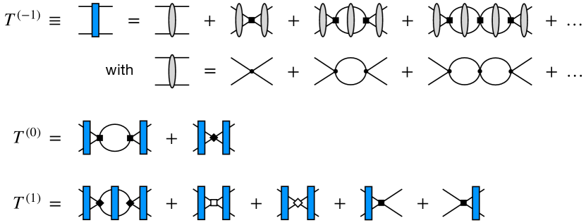
Figure 2: The leading, subleading and sub-subleading contributions to the P-wave scattering amplitude for the scenario of Eq. (2). Solid dots, rectangles and diamonds refer to the $C_{2}$-, $C_{4}$- and $C_{6}$-vertices, respectively. Open rectangles and open diamonds denote corrections to the $C_{4}$- and $C_{6}$-vertices proportional to $\delta C_{4}^{(3)}$ and $\delta C_{6}^{(1)}$ as explained in the text. For all diagrams, the two-particle Green’s functions refer to the usual nonrelativistic free resolvent operator as appears in Eq. (5).

Since no other diagram can contribute to the scattering length (for the employed renormalization conditions), the exact value of the LEC $C_{2}^{R}$ can be determined from matching $T_{C_{2}}(k,k,k)$ to $\big{[}T(k)/k^{2}\big{]}_{k=0}=4\pi a/m$, yielding

$$C_{2}^{R}(\mu_{3})=\frac{12\pi^{2}}{m(3\pi a^{-1}-2\mu_{3}^{3})}\,.$$ (24)

While $C_{2}^{R}$ is of natural size, its value had to be fine-tuned to reproduce $a^{-1}\sim M_{\rm lo}^{3}$, leading to the amplitude

$$T_{C_{2}}(p^{\prime},p,k)=-\frac{4\pi}{m}\frac{p^{\prime}p}{-\frac{1}{a}-\frac{2\mu_{1}}{\pi}k^{2}-ik^{3}}\;\sim\;\mathcal{O}(1)\,,$$ (25)

which is enhanced by two inverse powers of the soft scale relative to the expectation based on NDA. As a consequence, all diagrams made out of $m$ subleading vertices $\propto C_{4}$ and $m+1$ insertions of $T_{C_{2}}$, see the first line of Fig. 2, are enhanced and appear at the same order $\sim\mathcal{O}(1)$. Their resummed contribution defines the LO amplitude $T^{(-1)}(p^{\prime},p,k)\sim\mathcal{O}(M_{\rm lo}^{-1})$, which is additionally enhanced by one inverse power of $M_{\rm lo}$ as a result of the fine tuning of the value of $C_{4}^{R}$,

$$C_{4}^{R}(\mu_{1},\mu_{3})=\frac{9\pi^{2}(\pi r+4\mu_{1})}{4m\mu_{3}^{6}}\,,$$ (26)

needed to reproduce the effective range $r\sim M_{\rm lo}$. Notice that similarly to $C_{2}^{R}(\mu_{3})$, $C_{4}^{R}(\mu_{1},\mu_{3})\sim\mathcal{O}(1)$ is also consistent with NDA. The resulting LO amplitude reads

$$T^{(-1)}(p^{\prime},p,k) = -\frac{4\pi}{m}\,\frac{p^{\prime}p}{-\frac{1}{a}+\frac{1}{2}rk^{2}-ik^{3}+\frac{3\mu_{1}(\pi r+4\mu_{1})}{\pi\mu_{3}^{3}}k^{4}+i\frac{3(\pi r+4\mu_{1})}{2\mu_{3}^{3}}k^{5}+\mathcal{O}(k^{6})}$$ (27)

$$= -\frac{4\pi}{m}\,\frac{p^{\prime}p}{-\frac{1}{a}+\frac{1}{2}rk^{2}-ik^{3}}+\mathcal{O}(1)\,.$$

We emphasize that the obtained LO amplitude is, by construction, RG invariant at the considered level of accuracy since scale-dependent terms appear at order $\mathcal{O}(1)$.

Corrections to the LO amplitude emerge from diagrams involving insertions of vertices with a larger number of derivatives. As already pointed out above, the choice of higher-order operators is not unique. In particular, one can use any of the order-$M_{\rm lo}^{6}$ operators $p^{\prime 3}p^{3}$, $p^{\prime}p(p^{\prime 4}+p^{4})$, $p^{\prime}pk^{4}$ or $p^{\prime}p(p^{\prime 2}+p^{2})k^{2}$ as they are all equivalent on-shell. In addition to vertices involving higher powers of momenta, one has to take into account interactions emerging from higher-order corrections to the renormalized LECs. For example, the expression for $C_{4}^{R}$ in Eq. (26) is only correct up to terms of order $\sim M_{\rm lo}^{2}$, and one still needs to include the contributions from order-$M_{\rm lo}^{m}$ corrections $\delta C_{4}^{(m)}$ with $m=3,4,5,\ldots$. Alternatively and equivalently (up to higher-order terms), one can account for such corrections without introducing new vertices by re-adjusting the LECs $C_{n}^{R}$ at orders beyond the one they start contributing to the amplitude.

For the employed renormalization conditions, a diagram made out of $V_{i}$ vertices of type $i$ and order $d_{i}\geq 4$ with $N$ insertions of the LO amplitude in Eq. (27) contributes at order $M_{\rm lo}^{n}$ with

$$n=2-3N+\sum_{i}V_{i}(d_{i}-2)\geq\left\{\begin{array}[]{l}-1+\sum_{i}V_{i}(d_{i}-5)\\[4.0pt] 0\end{array}\right.\,,$$ (28)

where the upper inequality results from the condition $N\leq\sum_{i}V_{i}+1$. As for the lower inequality, we made use of the fact that diagrams made out of $m$ $C_{4}$-vertices and $m+1$ insertions of $T^{(-1)}$ are already included at LO. Thus, higher-order corrections $\propto C_{4}$ emerge from diagrams with at least two $C_{4}$-vertices separated by the free Green’s function, which start contributing at order $\sim M_{\rm lo}^{0}$. This shows that all contributions to the amplitude beyond LO are perturbative.

In Fig. 2, we show the contributions to the amplitude at next-to-leading order (NLO) and next-to-next-to-leading order (NNLO). Evaluating the two order-$M_{\rm lo}^{0}$ diagrams, where we have chosen to work with the operator $C_{6}p^{\prime 3}p^{3}$, we obtain the following contribution to the inverse $T$-matrix:

$$\frac{4\pi k^{2}}{m}\,\frac{T^{(0)}(k)}{\big{[}T^{(-1)}(k)\big{]}^{2}}=\left[-\frac{3(\pi r+4\mu_{1})^{2}}{8\pi\mu_{3}^{3}}+\frac{mC_{6}^{R}\mu_{3}^{6}}{9\pi^{3}}\right]k^{4}+\mathcal{O}(k^{6})\,.$$ (29)

Matching this expression to the first shape term in the ERE leads to

$$C_{6}^{R}(\mu_{1},\mu_{3})=\frac{9\pi^{2}[-48\mu_{1}^{2}+\pi(3\pi r^{2}+8v_{2}\mu_{3}^{3})]}{8m\mu_{3}^{9}}\;\sim\;\mathcal{O}(1)\,.$$ (30)

Similarly, for the NNLO contribution, we find

$$-\frac{4\pi k^{2}}{m}\left\{-\frac{T^{(1)}(k)}{\big{[}T^{(-1)}(k)\big{]}^{2}}+\frac{\big{[}T^{(0)}(k)\big{]}^{2}}{\big{[}T^{(-1)}(k)\big{]}^{3}}\right\} = \left[\frac{2\delta C_{4}^{(3)}\mu_{3}^{6}m}{9\pi^{3}}-\frac{3\left(4\mu_{1}+\pi r\right)}{2a\mu_{3}^{3}}\right]k^{2}\$$

$$+ \left[-\frac{9\mu_{1}\left(4\mu_{1}+\pi r\right)}{2a\mu_{3}^{6}}+\frac{\delta C_{6}^{(1)}\mu_{3}^{6}m}{9\pi^{3}}+\frac{4\delta C_{4}^{(3)}\mu_{1}\mu_{3}^{3}m}{3\pi^{3}}+\frac{3r\left(4\mu_{1}+\pi r\right)}{4\mu_{3}^{3}}\right]k^{4}$$

$$- \frac{i}{12\mu_{3}^{6}}\left[\frac{27\pi\left(4\mu_{1}+\pi r\right)}{a}-\frac{8\delta C_{4}^{(3)}\mu_{3}^{9}m}{\pi^{2}}+18\mu_{3}^{3}\left(4\mu_{1}+\pi r\right)\right]k^{5}+\mathcal{O}(k^{6})\,.$$

Matching this expression to the ERE leads to

$$\delta C_{4}^{(3)}(\mu_{1},\mu_{3}) = \frac{27\pi^{3}(\pi r+4\mu_{1})}{4am\mu_{3}^{9}}\,,$$

$$\delta C_{6}^{(1)}(\mu_{1},\mu_{3}) = -\frac{27\pi^{3}(\pi r+4\mu_{1})(6\mu_{1}+ar\mu_{3}^{3})}{4am\mu_{3}^{12}}\,.$$ (32)

Substituting these values back into the expression for the amplitude, the NNLO result finally takes the form

$$-\frac{4\pi k^{2}}{m}\left\{\frac{1}{T^{(-1)}(k)}-\frac{T^{(0)}(k)}{\big{[}T^{(-1)}(k)\big{]}^{2}}-\frac{T^{(1)}(k)}{\big{[}T^{(-1)}(k)\big{]}^{2}}+\frac{\big{[}T^{(0)}(k)\big{]}^{2}}{\big{[}T^{(-1)}(k)\big{]}^{3}}\right\} = -\frac{1}{a}+\frac{1}{2}rk^{2}-ik^{3}+v_{2}k^{4}+i\frac{9\pi(\pi r+4\mu_{1})}{4a\mu_{3}^{6}}k^{5}$$ (33)

$$+ \mathcal{O}(k^{6})\,.$$

Notice that the last term in the first line of this equation violates unitarity but is of order $\sim M_{\rm lo}^{8}$, which is beyond the accuracy of the NNLO approximation. Higher-order corrections to the amplitude can be calculated straightforwardly along the same lines and, for the case at hand, just restore the ERE.

As already pointed out above, we could have chosen the renormalization conditions by setting $\mu_{1}\sim M_{\rm lo}$, $\mu_{3}\sim M_{\rm hi}$ as an alternative to Eq. (21). Eq. (25) shows that in such an approach, the amplitude $T_{C_{2}}$ is even stronger enhanced relative to NDA, namely $T_{C_{2}}\sim M_{\rm lo}^{-1}$. On the other hand, the subleading interaction with $C_{4}^{R}\sim M_{\rm lo}$ is suppressed compared to NDA, reflecting directly the fine tuned value of the effective range $r\sim M_{\rm lo}$. Regardless of these changes, all diagrams in the first line of Fig. 2 contribute at the same order ($\sim M_{\rm lo}^{-1}$) and must be resummed to generate the LO amplitude $T^{(-1)}$. The perturbative expansion of the amplitude has the same form as before, but the corrections $\delta C_{4}$ and $\delta C_{6}$ are pushed to higher orders and need not be taken into account at NNLO.

The less fine-tuned scenario corresponding to Eq. (4) can be treated analogously. The LO contribution to the amplitude appears at order $\sim\mathcal{O}(1)$ from the same set of diagrams as visualized in Fig. 3. Notice that while the amplitude $T_{C_{2}}$ is enhanced by $\sim M_{\rm lo}^{-2}$ relative to NDA as a result of the fine-tuned value of $C_{2}^{R}$ in Eq. (24), the resummed contribution of diagrams shown in the first line of Fig. 3 is not enhanced any further since the value of $C_{4}^{R}$ is not fine-tuned. We further emphasize that differently to the EFT formulation with a dimer field Bedaque:2003wa , the LO amplitude is valid up-to-and-including order $M_{\rm lo}$ and already incorporates the term $-ik^{3}$ in the denominator stemming from the unitarity cut.

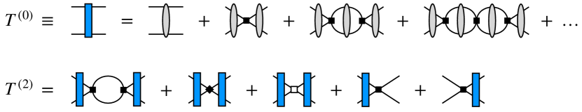
Figure 3: Diagrams contributing to the P-wave scattering amplitude up to order $M_{\rm lo}^{2}$ for the scenario of Eq. (4). Open rectangle denotes a correction to the $C_{4}$-vertex proportional to $\delta C_{4}^{(2)}$ as explained in the text. For further notation, see Fig. 2.

For the renormalization conditions specified in Eq. (21), corrections to the LO amplitude emerge from diagrams involving higher-order vertices and insertions of $T^{(0)}$, where the power counting expression (28) now takes the form

$$n=2-2N+\sum_{i}V_{i}(d_{i}-2)\geq\left\{\begin{array}[]{l}\sum_{i}V_{i}(d_{i}-4)\\[4.0pt] 2\end{array}\right.\,.$$ (34)

Evaluating the diagrams shown in the second line of Fig. 3 with $C_{2}^{R}$ and $C_{4}^{R}$ given in Eqs. (24), (26) and performing matching at the level of the ERE, the LEC $C_{6}^{R}$ is found to be

$$C_{6}^{R}(\mu_{1},\mu_{3})=\frac{9\pi^{2}\big{[}-36\pi\mu_{1}(\pi r+4\mu_{1})-3a(\pi r+4\mu_{1})^{2}\mu_{3}^{3}+8\pi av_{2}\mu_{3}^{6}\big{]}}{8am\mu_{3}^{12}}\;\sim\;\mathcal{O}(1)\,,$$ (35)

while the expression for $\delta C_{4}^{(2)}$ coincides with that of $\delta C_{4}^{(3)}$ in Eq. (III). The resulting expression for the inverse of the amplitude $T^{(0)}(k)+T^{(2)}(k)$ is then identical to the one given in Eq. (33).

While the doubly fine-tuned scenario of Eq. (2) only supports wide shallow resonances with ${\rm Re}\,k_{\rm res}\sim{\rm Im}\,k_{\rm res}\sim M_{\rm lo}$, where $k_{\rm res}$ denotes the location of the resonance pole, less fine-tuned systems described by Eq. (4) may feature narrow resonances with ${\rm Re}\,k_{\rm res}\sim M_{\rm lo}$, ${\rm Im}\,k_{\rm res}\sim M_{\rm lo}^{2}/M_{\rm hi}$. For the near-resonance kinematics with $k\sim{\rm Re}\,k_{\rm res}$, the LO amplitude $T^{(0)}(k)$ is enhanced and scales as $\sim M_{\rm lo}^{-1}$ rather than $\sim M_{\rm lo}^{0}$. In such a narrow kinematical region, the expansion of the amplitude actually coincides with that shown in Fig. 2 apart from the contribution of the $\delta C_{4}$-term, which appears already at NLO (i.e., in $T^{(0)}(k)$).

It should be understood that a perturbative calculation of the amplitude as demonstrated above is, strictly speaking, not necessary for the case of separable interactions considered here, since the LS equation can be solved exactly for the potential truncated at any order. In this way, one can obtain exact expressions for the renormalized LECs that incorporate all perturbative corrections $\delta C_{n}^{(s)}$ discussed above. For example, solving the LS equation for the potential given by the first two terms in Eq. (3), performing subtractive renormalization of the amplitude with $\mu_{5}=\mu_{7}=0$ and matching the LECs to reproduce the scattering length and effective range leads to

$$C_{2}^{R}(\mu_{3})=\frac{12\pi^{2}}{m(3\pi a^{-1}-2\mu_{3}^{3})}\,,\quad\quad C_{4}^{R}(\mu_{1},\mu_{3})=\frac{9\pi^{2}(\pi r+4\mu_{1})}{m(3\pi a^{-1}-2\mu_{3}^{3})^{2}}\,,$$ (36)

in agreement with Eqs. (24), (26) and (III). We further emphasize that choosing different renormalization conditions with $\mu_{\geq 5}\sim M_{\rm hi}$ would still result in the same (perturbative) expansion of the scattering amplitude after expressing the LECs in terms of physical parameters (i.e., coefficients in the ERE). One would, however, lose the manifest power counting for renormalized loop diagrams written in terms of the LECs $C_{n}^{R}$ $C_{n}^{m,R}$, as they would all appear to contribute at the same order.

The proposed EFT formulation can be straightforwardly generalized to resonant systems in partial waves with $l\geq 2$. Focussing again on the cases in which the effective range function has no poles for $k\sim M_{\rm lo}$, the strongest possible fine-tuning corresponds to the first $l+1$ terms in the ERE being suppressed compared to NDA and contributing at the same order as the unitary term, i.e. $a_{l}^{-1}\sim M_{\rm lo}^{2l+1}$, $r_{l}\sim M_{\rm lo}^{2l-1}$, $v_{2,\,l}\sim M_{\rm lo}^{2l-3}$, $\ldots$. A self-consistent Weinberg-like power counting scheme emerges by choosing the subtraction scales according to $\mu_{2l+1}\sim M_{\rm hi}$, $\mu_{2l+3}\sim\mu_{2l+5}\sim\ldots\sim M_{\rm lo}$. Choosing the remaining $\mu_{i}$’s of the order of the hard scale, i.e. $\mu_{1}\sim\mu_{3}\sim\ldots\sim\mu_{2l-1}\sim M_{\rm hi}$, will result in the renormalized LECs that all scale according to NDA. On the other hand, choosing some of these scales of the order $\sim M_{\rm lo}$ would lead to some of the LECs accompanying the interactions with $2l+2$ and more derivatives being suppressed. For $\mu_{1}\sim\mu_{3}\sim\ldots\sim\mu_{2l-1}\sim M_{\rm lo}$, the resulting scaling of the LECs $C_{2l+2}^{R}\sim M_{\rm lo}^{2l-1}$, $C_{2l+4}^{R}\sim M_{\rm lo}^{2l-3}$, $\ldots$ $C_{4l}^{R}\sim M_{\rm lo}$ is in a one-to-one correspondence with the scaling of the fine-tuned coefficients in the ERE.

Last but not least, we emphasize that the proposed EFT formulation is by no means restricted to the use of subtractive renormalization. Any regularization scheme that provides sufficient flexibility to incorporate the proper renormalization conditions is equally well suited for our purpose, and the results of the calculations are, of course, independent on the choice of regulator. For example, one can apply dimensional regularization in the partial wave basis (i.e., with the angular integrations being performed in $d=4$ space-time dimensions) as discussed in Ref. Phillips:1998uy . The regularized integrals $J_{2s+1}(k)$ with $s\geq l$ are then given by

$$J_{2s+1}(k)=\int\frac{l^{2}dl}{2\pi^{2}}\frac{ml^{2s}}{k^{2}-l^{2}+i\epsilon} \to \left(\frac{\mu}{2}\right)^{4-d}\int\frac{l^{2}d^{d-3}l}{2\pi^{2}}\frac{ml^{2s}}{k^{2}-l^{2}+i\epsilon}$$ (37)

$$= -\frac{m}{\pi}\left(\frac{\mu}{2}\right)^{4-d}k^{2s}(-k^{2}-i\epsilon)^{(d-3)/2}\;\Gamma\left(\frac{d-1}{2}\right)\Gamma\left(\frac{3-d}{2}\right)\,.$$

While both the standard MS/$\overline{\text{MS}}$ scheme and the PDS scheme of Ref. Kaplan:1998tg are too restrictive for the considered fine-tuned systems, one can introduce a generalized PDS approach, where poles in $d=3-2l$ dimensions,

$$J_{2s+1}(k)\Big{|}_{\rm pole}=\frac{mk^{2(s-l)}\mu^{2l+1}}{2^{2l}\pi\left[d-(3-2l)\right]}\,,$$ (38)

are subtracted from the analytically continued expressions for the loop integrals in $d$ dimensions by taking into account the corresponding counterterms (which are finite in $d=4$ dimensions). For the considered systems, the resulting scheme represents a particular case of the more general subtractive renormalization approach with all $\mu_{i}$ being set to zero except for $\mu_{2l+1}$, whose value is related to the DR scale $\mu$ via

$$\mu_{2l+1}=\left(2^{1-2l}\pi\right)^{1/(2l+1)}\mu\,.$$ (39)

Alternatively, one can also choose to additionally subtract poles in $3,\,1,\,\ldots,\,5-2l$ dimensions. In all cases, setting $\mu\sim M_{\rm hi}$ is necessary for the resulting EFT to feature a consistent power counting scheme as described above.

IV Wilsonian RG analysis

In the previous section, we have discussed in detail the formulation of halo EFT for resonant P-wave systems in terms of the renormalized potential. Below, we analyze the corresponding bare potentials by means of the Wilsonian RG flow equation following the philosophy of Refs. Birse:1998dk ; Birse:2009my ; Harada:2006cw and discuss the implications for the EFT.

IV.1 Wilsonian RG equation and fixed-point solutions for P-wave scattering

In Section III, we have presented a self-consistent formulation of the nonrelativistic EFT for resonant two-body P-wave scattering by short-range forces. The key element of our consideration was the knowledge of the general analytic structure of the on-shell scattering amplitude $T(k)$ parametrized in terms of the ERE, which allowed us to identify its expansion patterns for various scenarios and specify the appropriate renormalization conditions. The Wilsonian RG approach we discuss below aims to achieve similar goals, but from a different perspective and with no reliance upon the ERE. Instead, various expansion regimes corresponding to different physical situations are identified by studying the RG flow in the parameter space describing generic (bare) short-range potentials and analyzing perturbations around fixed-point solutions of the RG equation.

Following the philosophy of the Wilsonian RG analysis of Refs. Birse:1998dk ; Birse:2009my , we study the evolution of a theory, specified by an energy-dependent potential, upon continuously integrating out momentum modes above some cutoff scale $\Lambda$ while keeping the off-shell scattering amplitude unchanged. The running of the potential with the cutoff can be inferred from the LS equation for the off-shell $K$-matrix in the partial-wave basis

$$K(p^{\prime},p,k)=V(p^{\prime},p,k,\Lambda)+m\mathchoice{{\vbox{\hbox{$\textstyle-$}}\kern-4.86108pt}}{{\vbox{\hbox{$\scriptstyle-$}}\kern-3.25pt}}{{\vbox{\hbox{$\scriptscriptstyle-$}}\kern-2.29166pt}}{{\vbox{\hbox{$\scriptscriptstyle-$}}\kern-1.875pt}}\!\int_{0}^{\Lambda}\frac{l^{2}dl}{2\pi^{2}}\,\frac{V(p,l,k,\Lambda)\;K(l,p^{\prime},k)}{k^{2}-l^{2}}\,,$$ (40)

where the symbol $\mathchoice{{\vbox{\hbox{$\textstyle-$}}\kern-4.86108pt}}{{\vbox{\hbox{$\scriptstyle-$}}\kern-3.25pt}}{{\vbox{\hbox{$\scriptscriptstyle-$}}\kern-2.29166pt}}{{\vbox{\hbox{$\scriptscriptstyle-$}}\kern-1.875pt}}\!\int$ denotes the Cauchy principal value integral. The real $K$-matrix is related to the $T$-matrix considered in the previous sections via $1/K(p^{\prime},p,k)={\rm Re}[1/T(p^{\prime},p,k)]$. Taking the derivative with respect to $\Lambda$ and using the LS equation (40), we arrive at the differential equation

$$\frac{\partial V}{\partial\Lambda}=\frac{m}{2\pi^{2}}V(p^{\prime},\Lambda,k,\Lambda)\frac{\Lambda^{2}}{\Lambda^{2}-k^{2}}V(\Lambda,p,k,\Lambda)\,.$$ (41)

The RG equation emerges by expressing all dimensionful quantities in units of $\Lambda$ via $k=\hat{k}\Lambda$, $p=\hat{p}\Lambda$ and $p^{\prime}=\hat{p}^{\prime}\Lambda$ and introducing the rescaled dimensionless potential

$$\hat{V}(\hat{p}^{\prime},\hat{p},\hat{k},\Lambda)=\frac{m\Lambda}{2\pi^{2}}V(p^{\prime},p,k,\Lambda)\,,$$ (42)

defined in such a way that the factor of $m/(2\pi^{2})$ disappears from the LS equation. Expressing Eq. (41) in terms of the rescaled quantities then yields the RG equation Birse:1998dk ; Birse:2009my

$$\Lambda\frac{\partial\hat{V}}{\partial\Lambda}=\hat{p}^{\prime}\frac{\partial\hat{V}}{\partial\hat{p}^{\prime}}+\hat{p}\frac{\partial\hat{V}}{\partial\hat{p}}+\hat{k}\frac{\partial\hat{V}}{\partial\hat{k}}+\hat{V}+\hat{V}(\hat{p}^{\prime},1,\hat{k},\Lambda)\frac{1}{1-\hat{k}^{2}}\hat{V}(1,\hat{p},\hat{k},\Lambda)\,.$$ (43)

When lowering the cutoff towards $\Lambda\to 0$, the rescaled potential $\hat{V}$ becomes cutoff independent once $\Lambda$ is pushed well below all low-energy scales of the theory, i.e. the potential flows towards a fixed point solution $\hat{V}(\hat{p}^{\prime},\hat{p},\hat{k})$ that describes a scale-invariant system. Notice that the RG equation always possesses a trivial fixed point solution with $\hat{V}(\hat{p}^{\prime},\hat{p},\hat{k})=0$ corresponding to the vanishing $K$-matrix.

Since we are interested here in halo EFT with short-range interactions only, we can, without loss of generality, restrict ourselves to potentials of separable type. Nontrivial fixed points can then be constructed straightforwardly following the approach of Ref. Birse:2015iea . Specifically, consider rank-one separable potentials of the form $\hat{V}(\hat{p}^{\prime},\hat{p},\hat{k},\Lambda)=\hat{p}^{\prime}\hat{p}\,\hat{\omega}(\hat{k},\Lambda)$ as relevant for the case of P-wave scattering. A more general case of rank-two separable potentials is discussed in Appendix A. The RG equation (43) then turns into an ordinary differential equation for $\hat{\omega}(\hat{k},\Lambda)$, which becomes linear when expressed in terms of $[\hat{\omega}(\hat{k},\Lambda)]^{-1}$:

$$\Lambda\frac{\partial\hat{\omega}^{-1}}{\partial\Lambda}=\hat{k}\frac{\partial\hat{\omega}^{-1}}{\partial\hat{k}}-3\hat{\omega}^{-1}-\frac{1}{1-\hat{k}^{2}}\,.$$ (44)

Integrating this equation for the fixed-point solution with $\partial\hat{\omega}^{-1}/\partial\Lambda=0$, subject to the boundary condition that $\hat{\omega}(\hat{k})$ is an analytic function of $\hat{k}^{2}$ for $\hat{k}\ll 1$, leads to

$$\hat{\omega}_{\rm U}(\hat{k})=\frac{-6}{2+6\hat{k}^{2}-3\hat{k}^{3}\ln\frac{1+\hat{k}}{1-\hat{k}}}\,.$$ (45)

This fixed point is relevant for our considerations as it describes P-wave systems in the unitary limit with $1/K(p^{\prime},p,k)=0$.

The trivial and the unitary fixed points $\hat{V}_{\rm T}=0$ and $\hat{V}_{\rm U}$, in order, describe idealized situations we are not really interested in. Rather, we want to describe realistic systems that can be approximated by perturbations about these idealized cases. For such systems, the expansion patterns of the scattering amplitude in powers of the ratio of the soft and hard scales can be determined by analyzing perturbations about the fixed point solutions that scale with definite powers of $\Lambda$ Birse:1998dk . It is sufficient for our purposes to study purely energy-dependent perturbations of the form

$$\hat{\omega}(\hat{k},\Lambda)=\hat{\omega}(\hat{k})+\sum_{\nu}C_{\nu}\,\Lambda^{\nu}\phi_{\nu}(\hat{k})\,,$$ (46)

where the $C_{\nu}$ are dimensionful coefficients while the functions $\phi_{\nu}(\hat{k})$ and the powers $\nu$ are to be determined. A more general case of momentum-dependent perturbations can be studied along the lines of Ref. Birse:1998dk , but they generally appear to contribute at higher orders. Solving the linearized RG equation

$$\nu\phi_{\nu}=3\phi_{\nu}+\hat{k}\frac{\partial\phi_{\nu}}{\hat{k}}+2\frac{\hat{\omega}(\hat{k})}{1-\hat{k}^{2}}\phi_{\nu}\,,$$ (47)

subject to the constraint that the perturbations are analytic functions of $\hat{k}^{2}$ for $\hat{k}\ll 1$, one obtains

$$\phi_{\nu}(\hat{k}) = \hat{k}^{2n}\quad\text{with}\quad 2n=\nu-3=0,\,2,\,4,\,\ldots\,,\quad\text{for}\quad\hat{\omega}(\hat{k})=\hat{\omega}_{\rm T}(\hat{k})\,,$$

$$\phi_{\nu}(\hat{k}) = \hat{k}^{2n}[\hat{\omega}_{\rm U}(\hat{k})]^{2}\quad\text{with}\quad 2n=\nu+3=0,\,2,\,4,\,\ldots\,,\quad\text{for}\quad\hat{\omega}(\hat{k})=\hat{\omega}_{\rm U}(\hat{k})\,.$$ (48)

Notice that for perturbations around nontrivial fixed points such as $\hat{\omega}_{\rm U}(\hat{k})$, one can, alternatively to the linearized equation (47) for $\hat{\omega}(\hat{k},\Lambda)$, use the linear RG equation (44) for $[\hat{\omega}(\hat{k},\Lambda)]^{-1}$ Birse:2010fj to obtain

$$\frac{1}{\hat{\omega}(\hat{k},\Lambda)}=\frac{1}{\hat{\omega}_{\rm U}(\hat{k})}-\sum_{n=0}^{\infty}C_{2n-3}^{\prime}\Lambda^{2n-3}\hat{k}^{2n}\,,$$ (49)

where $C_{i}^{\prime}=C_{i}+\mathcal{O}(C^{2})$. From the point of view of the RG flow, the appearance of negative values of $\nu$ signals that the corresponding fixed point is unstable. For the unitary fixed point $\hat{\omega}_{\rm U}$, one has two relevant directions corresponding to $\nu=-3,\,-1$, see also Ref. Harada:2007ua , which bring the system away from $\hat{\omega}_{\rm U}$ when lowering the cutoff $\Lambda$. Potentials that do not reside on the critical surfaces of nontrivial fixed points flow in the $\Lambda\to 0$ limit towards the stable trivial fixed point, which possesses only irrelevant perturbations with $\nu>0$. In this deep infrared (IR) regime, the running of the potential is, therefore, controlled by the expansion around the trivial fixed point. If all dimensionless parameters $\hat{C}_{\nu}\equiv C_{\nu}/M_{\rm hi}^{\nu}$ that characterize the system are of order $\sim 1$ (as one would naturally expect since $M_{\rm hi}$ is the breakdown scale of the derivative expansion), the perturbative expansion of the potential around $V_{\rm T}=0$ as defined in Eqs. (46), (IV.1) also holds for $\Lambda\sim M_{\rm lo}$ and for $M_{\rm lo}\ll\Lambda\ll M_{\rm hi}$. Such situations describe weakly interacting “natural” P-wave systems, and the scattering amplitude can be calculated perturbatively.

An alternative expansion of the potential around the unitary fixed point

$$V(p^{\prime},p,k,\Lambda)=\frac{2\pi^{2}}{m\Lambda}\,\frac{p^{\prime}p}{\Lambda^{2}}\,\left\{\hat{\omega}_{\rm U}(k/\Lambda)+\left(\frac{M_{\rm hi}}{\Lambda}\right)^{3}\sum_{n=0}^{\infty}\hat{C}_{2n-3}\left(\frac{k}{M_{\rm hi}}\right)^{2n}\big{[}\hat{\omega}_{\rm U}(k/\Lambda)\big{]}^{2}\right\}$$ (50)

can be interpreted most easily by noticing the one-to-one correspondence of the inverse potential with $[\hat{\mbox{\boldmath$\omega$}}(k/\Lambda,\Lambda)]^{-1}$ fulfilling Eq. (49) with the ERE Birse:1998dk , which follows immediately if the LS equation is written in the operator form as $T^{-1}=V^{-1}+G_{0}$:

$$\frac{k^{2}}{K(k)}=-\frac{m}{4\pi}\left(-\frac{1}{a}+\frac{1}{2}rk^{2}+v_{2}k^{4}+\ldots\right)=-\frac{mM_{\rm hi}^{3}}{2\pi^{2}}\sum_{n=0}^{\infty}\hat{C}_{2n-3}^{\prime}\left(\frac{k}{M_{\rm hi}}\right)^{2n}\,.$$ (51)

The parameters $\hat{C}_{i}^{\prime}$ can thus be expressed in terms of the coefficients in the ERE:

$$\hat{C}_{-3}^{\prime}=-\frac{\pi}{2aM_{\rm hi}^{3}},\quad\quad\hat{C}_{-1}^{\prime}=\frac{\pi r}{4M_{\rm hi}},\quad\quad\hat{C}_{1}^{\prime}=\frac{\pi v_{2}M_{\rm hi}}{2},\quad\quad\ldots\,.$$ (52)

For an expansion around the unitary fixed point to be valid, the perturbations in Eq. (50) must be suppressed compared to the LO term corresponding to the unitary fixed point. For “natural” systems with all $\hat{C}_{\nu}\sim 1$, the irrelevant perturbations $\propto\hat{C}_{\nu}$ with $\nu>0$ are indeed small, but the relevant ones $\propto\hat{C}_{-3}$ and $\propto\hat{C}_{-1}$ are much larger than the first term in the curly brackets. Indeed, as we discussed above, “natural” systems rather correspond to the expansion around the trivial fixed point. However, for systems with the strength of the relevant perturbations being fine-tuned to unnaturally small values $a^{-1}\sim M_{\rm lo}^{3}$ and $r\sim M_{\rm lo}$ as given in Eq. (2), all perturbations in Eq. (50) are indeed suppressed compared to the LO term for $M_{\rm lo}\ll\Lambda\ll M_{\rm hi}$. Such systems reside close to the critical surface of the unitary fixed point, thus being attracted to $\hat{V}_{\rm U}$ for not too small values of $\Lambda$. For $\Lambda\sim M_{\rm lo}$, the two relevant perturbations become large and must be resummed. For even smaller cutoff values, these increasing perturbations drive the system towards the trivial fixed point. Notice that for the less fine-tuned scenario in Eq. (4), the relevant perturbations are not suppressed for any $\Lambda\ll M_{\rm hi}$. One, therefore, cannot expect such systems to be described by the expansion around the unitary fixed point.

To summarize, the Wilsonian RG analysis deals with the behavior of generic bare potentials in the IR regime with $\Lambda\ll M_{\rm hi}$. It allows one to identify certain expansion patterns of the scattering amplitude in powers of $M_{\rm lo}/M_{\rm hi}$ from analyzing the running of the potentials near the fixed points of the RG equation. For two-body scattering of nonrelativistic particles interacting via short-range forces we are interested in here, the RG analysis can be carried out analytically, yielding, however, essentially an alternative derivation of the ERE for the scattering amplitude. More interesting and nontrivial examples include applications of the RG analysis to systems interacting with both long- and short-range forces as relevant for chiral EFT for nuclear systems, see Refs. Barford:2002je ; Birse:2005um ; Birse:2007sx ; Ando:2008jb ; Birse:2010jr ; Harada:2010ba ; Harada:2013hwa ; Harada:2013zya for some work along this line.

IV.2 Implications for the EFT

While our considerations in the previous section in terms of the bare potentials have been rather general, they may appear unrelated to the subtractively renormalized formulation of halo EFT considered in Section III. The purpose of this section is to unmask the relationship between the two approaches and to address implications of the RG analysis to the power counting of the halo EFT.

To establish a connection between the two approaches, we consider the bare energy-dependent potential $V(p^{\prime},p,k)$ defined in Eq. (15) and corresponding to the subtractively renormalized potential $V^{R}(p^{\prime},p)=C_{2}^{R}p^{\prime}p+C_{4}^{R}p^{\prime}p(p^{\prime 2}+p^{2})$. To verify that it indeed complies with the expansions discussed in the previous section, it is more convenient to rewrite it in terms of the physical parameters $a$ and $r$ instead of $C_{2}^{R}$ and $C_{4}^{R}$. The resulting bare potential defines a family of physical systems characterized by the parameters $a$, $r$, $\mu_{1}$ and $\mu_{3}$. From the two remaining scales, $\mu_{7}$ is, in fact, a redundant parameter since the dependence of the amplitude on $\mu_{7}$ is completely eliminated by the running of the LEC $C_{2}^{R}$. Consequently, the potential does not depend on $\mu_{7}$ after being expressed in terms of $a$ and $r$. The scale $\mu_{5}$ does not enter the expression for the on-shell amplitude, cf. Eq. (14), but affects the off-shell behavior of the potential and scattering amplitude. For the sake of definiteness, we fix the off-shell behavior of the potential by choosing $\mu_{5}=0$ to obtain

$$V = -\frac{20\pi^{2}pp^{\prime}}{m}\bigg{[}840a\left(2a\mu_{3}^{3}-3\pi\right)^{3}-3a^{2}\left(4\mu_{1}+\pi r\right)\bigg{(}210\left(3\pi-2a\mu_{3}^{3}\right)^{2}\left(p^{2}+p^{\prime 2}\right)+\frac{9}{2}a^{2}\left(4\mu_{1}+\pi r\right)\bigg{\{}-35\left(k^{2}-p^{2}\right)$$ (53)

$$\times \left(k^{2}-p^{\prime 2}\right)\bigg{[}3k^{3}\ln\frac{\Lambda+k}{\Lambda-k}-6k^{2}(\Lambda-\mu_{1})-2(\Lambda^{3}-\mu_{3}^{3})\bigg{]}+42\Lambda^{5}\left(k^{2}-p^{2}-p^{\prime 2}\right)+30\Lambda^{7}\bigg{\}}\bigg{)}\bigg{]}$$

$$\times \bigg{[}42a^{2}\left(4\mu_{1}+\pi r\right)\left[5k^{2}(\Lambda^{3}-\mu_{3}^{3})+15k^{4}(\Lambda-\mu_{1})+3\Lambda^{5}\right]\left[9\pi\left(a^{2}\Lambda^{5}r-20\pi\right)+4a\left(9a\Lambda^{5}\mu_{1}-20a\mu_{3}^{6}+60\pi\mu_{3}^{3}\right)\right]$$

$$- 50a\left[3k^{2}(\Lambda-\mu_{1})+\Lambda^{3}-\mu_{3}^{3}\right]\left\{27\pi^{2}\left(a^{3}\Lambda^{7}r^{2}+56\pi\right)+8a\left[27a^{2}\Lambda^{7}\mu_{1}\left(2\mu_{1}+\pi r\right)-56a^{2}\mu_{3}^{9}+252\pi a\mu_{3}^{6}-378\pi^{2}\mu_{3}^{3}\right]\right\}$$

$$- 15ak^{3}\ln\frac{\Lambda+k}{\Lambda-k}\Big{(}8a\left\{27\mu_{1}\left[2a^{2}\Lambda^{5}\mu_{1}\left(7k^{2}-5\Lambda^{2}\right)+\pi k^{2}\left(7a^{2}\Lambda^{5}r-70\pi\right)-5\pi a^{2}\Lambda^{7}r\right]+280a^{2}\mu_{3}^{9}\right.$$

$$- \left.210a\mu_{3}^{6}\left[4ak^{2}\mu_{1}+\pi\left(ak^{2}r+6\right)\right]+630\pi\mu_{3}^{3}\left[4ak^{2}\mu_{1}+\pi\left(ak^{2}r+3\right)\right]\right\}-27\pi^{2}\left[a^{3}\Lambda^{5}r^{2}\left(5\Lambda^{2}-7k^{2}\right)\right.$$

$$+ \left.140\pi\left(ak^{2}r+2\right)\right]\Big{)}+1400\left(3\pi-2a\mu_{3}^{3}\right)^{4}\bigg{]}^{-1}\,.$$

Notice that since we want the corresponding rescaled potential to fulfill the RG equation, we have taken the limit $\Lambda\to\infty$ for the renormalized integrals $J_{n}^{R}(k,\mu_{i})$ in Eq. (15) to obtain the above expression. When inserted into the LS equation regularized with a sharp cutoff, the above potential yields the $\Lambda$-independent off-shell amplitude that reproduces Eq. (14) in the on-shell limit. It, therefore, fulfills Eq. (41) and may serve as a specific example of generic bare potentials considered in the previous section.

It is now instructive to expand this potential in the ratio of the soft and hard scales as defined in the RG analysis of Section IV.1. Specifically, we assign $\Lambda\sim k\sim p\sim p^{\prime}\sim M_{\rm lo}$ and choose $\mu_{3}\sim M_{\rm hi}$ to comply with the considered physical scenario by ensuring the absence of low-lying poles in the inverse on-shell $K$-matrix, see the discussion in Section III. As for the remaining scale $\mu_{1}$, we consider here the case of $\mu_{1}\sim M_{\rm hi}$, which allows one to simulate the correction to the potential needed to reproduce the shape parameter $v_{2}$ by tuning $\mu_{1}$.

• Consider first the doubly fine-tuned scenario of Eq. (2) with $a^{-1}\sim M_{\rm lo}^{3}$, $r\sim M_{\rm lo}$. Expanding the bare potential in Eq. (53), rescaled according to Eq. (42), in powers of $\epsilon\equiv M_{\rm lo}/M_{\rm hi}$, one obtains

  $$\hat{V}(\hat{p}^{\prime},\hat{p},\hat{k},\Lambda)=\frac{12\,\hat{p}^{\prime}\,\hat{p}}{-4+\frac{6\pi}{a\Lambda^{3}}-3\hat{k}^{2}\big{(}4+\frac{\pi r}{\Lambda}\big{)}+6\hat{k}^{3}\ln\frac{1+\hat{k}}{1-\hat{k}}}+\frac{432\,\hat{k}^{4}\,\hat{p}^{\prime}\,\hat{p}\,\mu_{1}^{2}\,\Lambda}{\Big{[}-4+\frac{6\pi}{a\Lambda^{3}}-3\hat{k}^{2}\big{(}4+\frac{\pi r}{\Lambda}\big{)}+6\hat{k}^{3}\ln\frac{1+\hat{k}}{1-\hat{k}}\Big{]}^{2}\mu_{3}^{3}}+\mathcal{O}(\epsilon^{2})\,.$$ (54)

  In agreement with the considerations of Section IV.1, cf. the second line in Eq. (IV.1), the potential is described in terms of the expansion around the unitary fixed point with resummed corrections stemming from the relevant perturbations $\propto a^{-1},r$. The LO term $\hat{V}^{(0)}$ leads to the effective range approximation $k^{3}\cot\delta=-a^{-1}+rk^{2}/2$, while the order-$\epsilon$ correction $\hat{V}^{(1)}$ generates the first shape term in the ERE if one chooses $\mu_{1}^{2}=\pi v_{2}\mu_{3}^{3}/6$ as mentioned above. Notice that the LO term corresponds to the theory that parametrizes the renormalized trajectories connecting the unitary and trivial fixed points, see Appendix A for more details.

• For the less fine-tuned scenario of Eq. (4) with $a^{-1}\sim M_{\rm lo}^{2}M_{\rm hi}$ and $r\sim M_{\rm hi}$, the expansion of the potential takes the form

  $$\hat{V}(\hat{p}^{\prime},\hat{p},\hat{k},\Lambda)=\frac{4\hat{p}^{\prime}\hat{p}}{\pi\left(\frac{2}{a\Lambda^{3}}-\frac{r}{\Lambda}\hat{k}^{2}\right)}+\frac{8\hat{p}^{\prime}\hat{p}}{3\pi^{2}\left(\frac{2}{a\Lambda^{3}}-\frac{r}{\Lambda}\hat{k}^{2}\right)^{2}}\left(2+6\hat{k}^{2}-3\hat{k}^{3}\ln\frac{1+\hat{k}}{1-\hat{k}}\right)+\mathcal{O}(\epsilon^{3})\,,$$ (55)

  where the first and second terms contribute at orders $\epsilon$ and $\epsilon^{2}$, respectively. As expected from the general arguments of the previous section, this situation corresponds to the expansion around the trivial fixed point with resummed contributions from the scattering length and effective range. In this case, the LO potential $\hat{V}^{(1)}$ yields

  $$k^{3}\cot\delta=\left(-\frac{1}{a}-\frac{2\Lambda^{3}}{3\pi}\right)+\left(\frac{r}{2}-\frac{2\Lambda}{\pi}\right)k^{2}+\frac{2k^{4}}{\pi\Lambda}+\ldots\,,$$ (56)

  thus indeed providing the LO contribution to the ERE, accompanied with higher-order contributions.

One may now raise the question of what the expansion of the potential would correspond to if all subtraction scales, including $\mu_{3}$, would have been chosen of the order of the soft scale in the problem, such that the scattering amplitude would feature low-lying zero(s). As shown in Appendix A, the resulting resonant systems are described by expansions around different unstable fixed points.

The above examples show that for nonrelativistic systems with a clear scale separation, low-energy physics can be systematically described by expanding the bare potential around fixed point solutions of the RG equation. This method utilizes the same kind of expansion in powers of $M_{\rm lo}/M_{\rm hi}$ as the corresponding EFT, and it has proven to be particularly useful for analyzing universality aspects of strongly interacting systems, see Ref. Braaten:2004rn ; Naidon:2016dpf for review articles. In spite of the similarities, the RG approach outlined above does not directly translate into the EFT program in the way it is usually formulated, which relies on (local) effective Lagrangians and typically requires choosing $\Lambda\sim M_{\rm hi}$ to exploit the full predictive power. The scattering length and effective range entering the bare potential in Eq. (53), which obeys a well-defined expansion around the unitary fixed point as given in Eq. (54), are, in fact, complicated nonlinear functions of the parameters entering the effective Lagrangian, i.e. of the renormalized LECs $C_{2}^{R}(\mu_{i})$ and $C_{4}^{R}(\mu_{i})$, and the expansion pattern of the renormalized potential and thus also of the scattering amplitude depends crucially on the choice of the scales $\mu_{i}$ (i.e. on the renormalization conditions), see Section III for details, which play a role similar to the floating cutoff $\Lambda$ in the Wilsonian RG analysis. For S-wave systems near the unitary limit, all renormalization scale(s) can be pushed down to $\mu_{i}\sim M_{\rm lo}$ as done in the KSW approach, and the correspondence between the Wilsonian and Gell-Mann and Low RG approaches becomes evident. The scaling behavior of the perturbations in the bare potential, expanded around the unitary fixed point, then translates into the scaling of the renormalized LECs in the KSW approach. The Wilsonian RG analysis thus provides an alternative derivation of the KSW power counting. On the other hand, for resonant P-wave systems we are interested in here, with the coefficients in the ERE scaling according to Eqs. (2) and (4), choosing $\mu_{3}\sim M_{\rm lo}$ corresponds, as already mentioned above, to a different class of theories, see Appendix A for details. Thus, no KSW-like power counting scheme with the LECs $C_{6}^{R}$, $C_{8}^{R}$, $\ldots$ being enhanced compared to their NDA scaling by the factor of $M_{\rm lo}^{-6}$, as suggested by Eq. (50), can be formulated for the case at hand. The contributions of these operators to the amplitude are, of course, still enhanced for resonant systems regardless of the choice of the renormalization conditions (as follows from both the ERE and the Wilsonian RG analysis). In the Weinberg-like power counting scheme formulated in Section III, all LECs scale according to NDA and the large anomalous canonical dimensions of the corresponding operators are generated through the choice of the renormalization conditions ($\mu_{3}\sim M_{\rm hi}$), see also Ref. Harada:2006cw for a related discussion.

Last but not least, we emphasize that the essential ingredient of the Wilsonian RG method outlined above is its restriction to the IR regime with $\Lambda\ll M_{\rm hi}$, where the representation of the effective potential in terms of the expansion in powers of momenta is valid. It cannot provide a systematic power counting for the bare potential if the cutoff parameter is taken beyond the hard scale of the problem. This is further illustrated in Appendix B, where the exact RG trajectory for a toy-model S-wave potential with long-range interaction is calculated numerically. Generally, moving against the RG flow by increasing $\Lambda$ beyond the hard scales of the problem, without at the same time taking into account the corresponding new degrees of freedom, as it is done in the lcRG-invariant approach, is a dangerous endeavor. It typically leads to complex values of the potential when written in terms of the LECs or brings it to infinity for $\Lambda\to\infty$ (unless the theory lies on a critical surface of some nontrivial fixed point).

V Summary and conclusions

In this paper we have revisited the problem of renormalization in low-energy EFTs of nuclear interactions on the example of resonant P-wave scattering. Following Refs. Bertulani:2002sz ; Bedaque:2003wa , we focused here on the fine-tuned scenarios with the coefficients in the effective range expansion scaling according to Eqs. (2) or (4) and leading to the appearance of shallow bound, virtual or resonance states. While such resonant systems have already been extensively studied using EFT formulations with auxiliary dimer fields Bertulani:2002sz ; Bedaque:2003wa ; Gelman:2009be ; Alhakami:2017ntb ; Schmidt:2018vvl ; Ji:2014wta ; Ryberg:2017tpv ; Soto:2007pg , see Ref. Hammer:2017tjm for a review article, we have employed here the effective Lagrangian written solely in terms of contact interactions. Our main findings are summarized below.

• We started with applying the lcRG-invariant approach of Refs. Hammer:2019poc ; Valderrama:2016koj ; Habashi:2020qgw to resonant P-wave scattering in Section II. The presence of shallow states demands resummation of the contact interactions $C_{2}p^{\prime}p$ and $C_{4}p^{\prime}p(p^{\prime 2}+p^{2})$ when calculating the scattering amplitude. However, solving the Lippmann-Schwinger equation and expressing the bare LECs $C_{2}(\Lambda)$ and $C_{4}(\Lambda)$ in terms of the scattering length and effective range, we found no solutions in terms of real LECs compatible with either of Eqs. (2) and (4) if the cutoff is taken well beyond the hard scale in the problem, $\Lambda\gg M_{\rm hi}$. This result is in agreement with the causality bounds derived in Ref. Hammer:2010fw , but it appears to contradict the conclusions obtained using the EFT with auxiliary dimer fields Bertulani:2002sz ; Bedaque:2003wa ; Hammer:2017tjm . Indeed, keeping $\Lambda\sim M_{\rm hi}$ shows that at least the less fine-tuned scenario of Eq. (4) is easily realizable in terms of a simple quantum mechanical model, while it cannot be accommodated by the lcRG-invariant approach.

• The above issue with the lcRG-invariant approach can be traced back to the inconsistent (from the EFT point of view) renormalization of the LS equation with perturbatively non-renormalizable potentials, which requires the inclusion of an infinite number of counterterms, see e.g. Ref. Epelbaum:2018zli . As repeatedly pointed out in Refs. Lepage:1997cs ; Epelbaum:2009sd ; Epelbaum:2017byx ; Epelbaum:2018zli ; Epelbaum:2020maf , arbitrarily large cutoff values can be employed in a way compatible with the principles of EFT only after all UV divergences, generated by iterations of the LS equation, are removed. In Section III, we have shown how to consistently renormalize the scattering amplitude for resonant P-wave scattering in halo EFT with no auxiliary fields using a subtractive scheme and utilizing the usual QFT renormalization technique to all orders in the loop expansion. A separable form of the underlying effective potential admits a closed-form expression for the (infinite set of) counterterms needed to absorb all divergences in the LS equation as given in Eq. (15). The resulting scattering amplitude is finite in the limit $\Lambda\to\infty$, both perturbatively (i.e., at any order in the loop expansion) and non-perturbatively. A self-consistent power counting scheme is obtained by choosing the subtraction scales according to $\mu_{3}\sim M_{\rm hi}$, $\mu_{5}\sim\mu_{7}\sim M_{\rm lo}$. These renormalization conditions ensure that (i) all renormalized LECs scale according to NDA, (ii) the renormalized contributions of diagrams obey manifest power counting, and their EFT order can be determined a priori using the power counting formulas (28) and (34) for the doubly and singly fine-tuned scenarios of Eqs. (2) and (4), respectively, (iii) the renormalized LECs $C_{2}^{R}$ and $C_{4}^{R}$ can be expressed in terms of $a$ and $r$ regardless of their actual values in a close analogy with the EFT formulations of Refs. Bertulani:2002sz ; Bedaque:2003wa , (iv) the residual dependence of the amplitude on the subtraction scales $\mu_{i}$ is beyond the actual order of the calculation and (v) the EFT expansion is compatible with the required scenarios in Eqs. (2) and (4). The choice of the scale $\mu_{3}\sim M_{\rm hi}$ is dictated by the need to avoid the appearance of low-lying amplitude zeros to comply with the assumed scaling behaviors in Eqs. (2) and (4). It is, therefore, not possible to formulate a KSW-like power counting scheme for the considered systems, where all subtraction scales would be chosen of the order of $M_{\rm lo}$ and the enhancement of the resummed LO contribution to the amplitude would emerge from the enhancement of the individual diagrams through the enhanced renormalized LECs.

  The EFT we propose is not restricted to P-waves and can be straightforwardly generalized to describe resonant systems with any value of the orbital angular momentum. It also permits the use of dimensional regularization, supplied with an appropriate subtraction scheme that allows sufficient flexibility to implement the proper renormalization conditions, such as e.g. the generalized PDS scheme. This feature might be particularly beneficial for applications to halo systems in the presence of external electroweak probes.

• Next, we have performed a Wilsonian RG analysis of P-wave scattering in Section IV following the philosophy of Refs. Birse:1998dk ; Birse:2009my , see also Refs. Harada:2006cw ; Harada:2007ua for a closely related approach. Our main motivation here was to clarify the relationship between this powerful method, formulated in terms of bare potentials, and the subtractively renormalized halo EFT framework developed in Section III. The key ingredient of the Wilsonian RG analysis is the search for fixed point solutions of the RG equation (43). In addition to the trivial fixed point that describes non-interacting systems, the unitary fixed point in Eq. (45) plays an important role for doubly fine-tuned systems specified in Eq. (2). This unstable fixed point describes scale-free P-wave systems with $a^{-1}\to 0$ and $r\to 0$ and has two relevant directions Harada:2007ua . Once the floating cutoff $\Lambda$ is lowered well below the hard scale $M_{\rm hi}$, so that the expansion of the potential in terms of contact interactions is valid, all theories describing doubly fine-tuned systems in Eq. (2) get attracted by the unitary fixed point when $M_{\rm lo}\lesssim\Lambda\ll M_{\rm hi}$. This allows one to identify a systematic and universal expansion of the scattering amplitude for such fine-tuned systems by analyzing the scaling of perturbations around the fixed point for $\Lambda\sim M_{\rm lo}$. For the case at hand, the Wilsonian RG analysis merely provides an alternative derivation of the ERE, cf. Eq. (51). It also implies that the contributions of the shape-terms to the scattering amplitude for doubly fine-tuned systems are enhanced by $M_{\rm lo}^{-6}$ as compared with NDA, see Eq. (50). This is, of course, in agreement with the ERE and, therefore, also with the EFT formulated in Section III as visualized in Fig. 2. On the other hand, the behavior of singly fine-tuned systems specified in Eq. (4) is not expected to be governed by the expansion around the unitary fixed point.

  To further demonstrate the close relationship between the two approaches, we have considered the potential in Eq. (15), which includes the resummed contributions of the counterterms in the subtractively renormalized EFT framework. After taking the limit $\Lambda\to\infty$ in the renormalized UV-convergent integrals $J_{n}^{R}$, the resulting rescaled bare potential fulfills the RG equation (43). We have explicitly verified that the RG flow of this potential indeed coincides with the expansion around the unitary fixed point for $\Lambda\sim M_{\rm lo}$, provided $\mu_{3}$ is chosen of the order $\sim M_{\rm hi}$ to comply with the conditions of Eq. (2). For singly fine-tuned systems specified in Eq. (4), the expansion of the potential in powers of $M_{\rm lo}/M_{\rm hi}$ for $\Lambda\sim M_{\rm lo}$ is found to coincide with that around the trivial fixed point with resummed corrections $\propto a^{-1},\,r$. The general RG flow of rank-two separable potentials like the one in Eq. (53) is discussed in Appendix A and shown to exhibit a rather rich structure.

  Last but not least, we emphasize that taking $\Lambda\sim M_{\rm hi}$ or larger is not compatible with the systematics underlying approximate expansions of the bare potential within the Wilsonian RG analysis. To illustrate this point, we compared in Appendix B the exact RG flow for a toy-model S-wave potential, featuring a long-range interaction, to the approximate result obtained using the lcRG-invariant approach. Fixing one available parameter of the LO contact interaction as a function of $\Lambda$ from the phase shift at some fixed energy, the resulting low-energy phase shifts are found to show very mild cutoff-dependence for $\Lambda\gg M_{\rm hi}$, thus (approximately) satisfying the condition of the RG invariance of the lcRG-invariant approach. However, the obtained limit-cycle-like $\Lambda$-dependence of the LO potential disagrees with the smooth RG flow behavior of the underlying model, a result that might have been expected given that the LO approximation to the bare potential is only valid for $\Lambda$ below $M_{\rm hi}$.

Previous halo EFT studies of resonant systems in P- and higher partial waves made use of the formulations with auxiliary dimer fields Bertulani:2002sz ; Bedaque:2003wa ; Gelman:2009be ; Alhakami:2017ntb ; Hammer:2017tjm , which are usually claimed to be introduced for convenience, see e.g. Ref. Hammer:2019poc . In this paper we have explicitly shown that the EFT formulations with and without dimer fields are indeed equivalent. A remarkable aspect of this equivalence is that all diagrams contributing to the LO scattering amplitude in halo EFT with auxiliary dimer fields are renormalizable, since all divergences from dressing the dimeron propagator can be absorbed into its residual mass and the particle-dimeron coupling constant. In contrast, the effective potential involving contact interactions in the formulation without auxiliary fields is not renormalizable in the usual sense. A proper renormalization of the scattering amplitude, therefore, requires taking into account contributions of an infinite number of counterterms. This unavoidably introduces a dependence on the subtraction scales in the renormalized amplitude, which reflects the freedom in choosing the finite pieces of the corresponding coupling constants and can be kept to be of a higher order by using the appropriate renormalization conditions as discussed in Section III. The resulting subtractively renormalized EFT is indeed equivalent to halo EFT with auxiliary fields. On the other hand, we have shown that these two EFT formulations are not equivalent to the lcRG-invariant approach of Refs. Nogga:2005hy ; Hammer:2019poc ; Valderrama:2016koj ; Habashi:2020qgw if the requirement of $\Lambda\gg M_{\rm hi}$ is to be taken seriously.

Appendix A RG flow for rank-two separable P-wave potentials

The purpose of this appendix is to provide a detailed discussion of the RG invariant bare potential of Section IV.2 and its interpretation from the point of view of the RG flow. To this aim, we consider a more general class of energy-dependent potentials as compared to our considerations in Section IV.1 of a rank-two separable form:

$$V(p^{\prime},p,k,\Lambda)=\mbox{\boldmath$\chi$}^{T}(p^{\prime})\,\mbox{\boldmath$\omega$}(k,\Lambda)\,\mbox{\boldmath$\chi$}(p)\,\quad\quad\text{with}\quad\mbox{\boldmath$\chi$}(p)=(p,p^{3})^{T}\,.$$ (57)

Here and in what follows, symbols in bold refer to matrix-valued functions. In particular, $\omega$ is a real $2\times 2$ matrix that depends on the cutoff $\Lambda$ and the on-shell momentum $k$. This is the type of potential we used to compute the LO scattering amplitude for resonant P-wave systems in section III, cf. Eq. (15).

We consider a generic bare potential as defined in Eq. (57), which is required to yield a cutoff-independent off-shell scattering amplitude and thus fulfills Eq. (41). Following Ref. Birse:2015iea , we derive nontrivial fixed-point solutions of the RG equation (43) for the rescaled potential $\hat{V}(\hat{p}^{\prime},\hat{p},\hat{k})$. We start with rewriting Eq. (43) in the form of the matrix equation for $\hat{\mbox{\boldmath$\omega$}}(\hat{k},\Lambda)$ defined via $\hat{V}(\hat{p}^{\prime},\hat{p},\hat{k},\Lambda)=:\mbox{\boldmath$\chi$}^{T}(\hat{p}^{\prime})\,\hat{\mbox{\boldmath$\omega$}}(\hat{k},\Lambda)\,\mbox{\boldmath$\chi$}(\hat{p})$:

$$\Lambda\frac{\partial\hat{\mbox{\boldmath$\omega$}}}{\partial\Lambda}=\left(\begin{array}[]{cc}1&0\\ 0&3\end{array}\right)\hat{\mbox{\boldmath$\omega$}}+\hat{\mbox{\boldmath$\omega$}}\left(\begin{array}[]{cc}1&0\\ 0&3\end{array}\right)+\hat{k}\frac{\partial\hat{\mbox{\boldmath$\omega$}}}{\partial\hat{k}}+\hat{\mbox{\boldmath$\omega$}}+\hat{\mbox{\boldmath$\omega$}}\frac{{\mbox{\boldmath$\chi$}}(1)\,{\mbox{\boldmath$\chi$}}^{T}(1)}{1-\hat{k}^{2}}\hat{\mbox{\boldmath$\omega$}}\,.$$ (58)

For invertible matrices $\hat{\mbox{\boldmath$\omega$}}$, the above RG equation can be rewritten into a linear differential equation for $\hat{\mbox{\boldmath$\omega$}}^{-1}$:

$$-\Lambda\frac{\partial\hat{\mbox{\boldmath$\omega$}}^{-1}}{\partial\Lambda}=\hat{\mbox{\boldmath$\omega$}}^{-1}\left(\begin{array}[]{cc}1&0\\ 0&3\end{array}\right)+\left(\begin{array}[]{cc}1&0\\ 0&3\end{array}\right)\hat{\mbox{\boldmath$\omega$}}^{-1}-\hat{k}\frac{\partial\hat{\mbox{\boldmath$\omega$}}^{-1}}{\partial\hat{k}}+\hat{\mbox{\boldmath$\omega$}}^{-1}+\frac{{\mbox{\boldmath$\chi$}}(1)\,{\mbox{\boldmath$\chi$}}^{T}(1)}{1-\hat{k}^{2}}\,,$$ (59)

which reduces to the uncoupled first-order partial differential equations for the components of the matrix $\hat{\mbox{\boldmath$\omega$}}^{-1}$:

$$-\Lambda\frac{\partial\hat{\omega}_{11}^{-1}}{\partial\Lambda} = 3\hat{\omega}_{11}^{-1}-\hat{k}\frac{\partial\hat{\omega}_{11}^{-1}}{\partial\hat{k}}+\frac{1}{1-\hat{k}^{2}}\,,$$

$$-\Lambda\frac{\partial\hat{\omega}_{12}^{-1}}{\partial\Lambda} = 5\hat{\omega}_{12}^{-1}-\hat{k}\frac{\partial\hat{\omega}_{12}^{-1}}{\partial\hat{k}}+\frac{1}{1-\hat{k}^{2}}\,,$$

$$-\Lambda\frac{\partial\hat{\omega}_{22}^{-1}}{\partial\Lambda} = 7\hat{\omega}_{22}^{-1}-\hat{k}\frac{\partial\hat{\omega}_{22}^{-1}}{\partial\hat{k}}+\frac{1}{1-\hat{k}^{2}}\,.$$ (60)

Here, we restrict ourselves to Hermitian potentials, so that $\hat{\omega}_{12}^{-1}=\hat{\omega}_{21}^{-1}$. For $\Lambda$-independent $\hat{\mbox{\boldmath$\omega$}}$, we can easily integrate these equations, subject to the boundary condition that $\hat{\omega}^{-1}_{ij}(\hat{k})$ are analytic functions of $\hat{k}^{2}$, to obtain the potential corresponding to the rank-two fixed-point solution of the RG equation

$$\hat{V}_{\rm rank-2}(\hat{p}^{\prime},\hat{p},\hat{k}) = \left(\hat{p}^{\prime},\hat{p}^{\prime 3}\right)\left(\begin{array}[]{cc}{\rm Re}\,\hat{J}_{3}(\hat{k})&{\rm Re}\,\hat{J}_{5}(\hat{k})\\[4.0pt] {\rm Re}\,\hat{J}_{5}(\hat{k})&{\rm Re}\,\hat{J}_{7}(\hat{k})\end{array}\right)^{-1}\left(\begin{array}[]{c}\hat{p}\\[4.0pt] \hat{p}^{3}\end{array}\right)$$ (65)

$$= -\frac{5\hat{p}^{\prime}\hat{p}}{5-7\hat{k}^{2}}\left[7\left(\hat{k}^{2}-\hat{p}^{\prime 2}\right)\left(\hat{k}^{2}-\hat{p}^{2}\right)+\frac{6\left(5-7\hat{p}^{\prime 2}\right)\left(5-7\hat{p}^{2}\right)}{8+80\hat{k}^{2}-210\hat{k}^{4}-15\hat{k}^{3}\left(5-7\hat{k}^{2}\right)\ln\frac{1+\hat{k}}{1-\hat{k}}}\right]\,,$$ (66)

where the rescaled dimensionless integrals $\hat{J}_{n}(\hat{k})$ are defined in terms of the integrals $J_{n}(k)$ from Eq. (6) via

$$\hat{J}_{n}(\hat{k})=\frac{2\pi^{2}}{m}\frac{1}{\Lambda^{n}}J_{n}(\hat{k}\Lambda)\,.$$ (67)

Notice that apart from $\hat{V}_{\rm rank-2}(\hat{p}^{\prime},\hat{p},\hat{k})$ and the trivial potential $\hat{V}_{\rm T}(\hat{p}^{\prime},\hat{p},\hat{k})=0$, any potential corresponding to a non-invertible matrix $\hat{\mbox{\boldmath$\omega$}}(\hat{k})$ with $\det\hat{\mbox{\boldmath$\omega$}}(\hat{k})=0$ also represents a fixed-point solution of the RG equation (which corresponds to $K(k)=0$). Interestingly, if one drops the second term in the squared brackets of Eq. (65), the resulting scale-free potential corresponds to such a fixed-point solution of the RG equation with a non-invertible matrix $\hat{\mbox{\boldmath$\omega$}}(\hat{k})$.

The above rank-two separable fixed point has nine relevant perturbations, which can be parametrized by some (dimensionful) quantities $\alpha_{1},\,\alpha_{2},\,\ldots,\,\alpha_{9}$. The resulting RG-invariant rescaled potential with resummed relevant perturbations can be written in the form

$$\hat{V}(\hat{p}^{\prime},\hat{p},\hat{k},\Lambda)=\left(\hat{p}^{\prime},\hat{p}^{\prime 3}\right)\left(\begin{array}[]{ccc}\frac{\alpha_{1}}{\Lambda^{3}}+\frac{\alpha_{2}}{\Lambda}\hat{k}^{2}+{\rm Re}\,\hat{J}_{3}(\hat{k})&&\frac{\alpha_{3}}{\Lambda^{5}}+\frac{\alpha_{4}}{\Lambda^{3}}\hat{k}^{2}+\frac{\alpha_{5}}{\Lambda}\hat{k}^{4}+{\rm Re}\,\hat{J}_{5}(\hat{k})\\[6.0pt] \frac{\alpha_{3}}{\Lambda^{5}}+\frac{\alpha_{4}}{\Lambda^{3}}\hat{k}^{2}+\frac{\alpha_{5}}{\Lambda}\hat{k}^{4}+{\rm Re}\,\hat{J}_{5}(\hat{k})&&\frac{\alpha_{6}}{\Lambda^{7}}+\frac{\alpha_{7}}{\Lambda^{5}}\hat{k}^{2}+\frac{\alpha_{8}}{\Lambda^{3}}\hat{k}^{4}+\frac{\alpha_{9}}{\Lambda}\hat{k}^{6}+{\rm Re}\,\hat{J}_{7}(\hat{k})\end{array}\right)^{-1}\left(\begin{array}[]{c}\hat{p}\\[6.0pt] \hat{p}^{3}\end{array}\right)\,,$$ (68)

and corresponds to the on-shell $K$-matrix

$$\frac{2\pi^{2}k^{2}}{m\,K(k)}=\alpha_{1}+\alpha_{2}k^{2}-\frac{\left\{\alpha_{3}+k^{2}\left[-\alpha_{1}+\alpha_{4}+\left(\alpha_{5}-\alpha_{2}\right)k^{2}\right]\right\}{}^{2}}{\alpha_{6}+k^{2}\left\{-2\alpha_{3}+\alpha_{7}+k^{2}\left[\alpha_{1}-2\alpha_{4}+\alpha_{8}+\left(\alpha_{2}-2\alpha_{5}+\alpha_{9}\right)k^{2}\right]\right\}}\,.$$ (69)

It is not hard to see that the RG-invariant bare potential corresponding to the subtractively renormalized scattering amplitude considered in Sections III and IV.2, i.e. the potential given in Eq. (15) with $J_{n}^{R}$ being replaced by $J_{n}^{R,\;\infty}\equiv\lim_{\Lambda\to\infty}J_{n}^{R}$, represents a special case of Eq. (68) with

$$\alpha_{1}=\alpha_{4}=\alpha_{8}=\frac{\mu_{3}^{3}}{3}\,,\quad\alpha_{2}=\alpha_{5}=\alpha_{9}=\mu_{1}\,,\quad\alpha_{7}=\frac{\mu_{5}^{5}}{5}\,,\quad\alpha_{3}=\frac{1}{5\tilde{C}_{4}^{R}}+\frac{\mu_{5}^{5}}{5}\,,\quad\alpha_{6}=-\frac{\tilde{C}_{2}^{R}}{5(\tilde{C}_{4}^{R})^{2}}+\frac{\mu_{7}^{7}}{7}\,.$$ (70)

The last two equalities show that the “couplings” $\mu_{5}$ and $\mu_{7}$ are indeed redundant as already pointed out in Section IV.2. Alternatively, following the procedure of that section, one can choose to parametrize the theory directly in terms of the physical parameters $a^{-1}$, $r$ instead of the LECs $C_{2}^{R}$, $C_{4}^{R}$. For $\mu_{5}=0$, Eq. (70) then turns to

$$\alpha_{1}=\alpha_{4}=\alpha_{8}=\frac{\mu_{3}^{3}}{3}\,,\quad\alpha_{2}=\alpha_{5}=\alpha_{9}=\mu_{1}\,,\quad\alpha_{7}=0\,,\quad\alpha_{3}=\frac{2(3\pi a^{-1}-2\mu_{3}^{3})^{2}}{9(\pi r+4\mu_{1})}\,,\quad\alpha_{6}=-\frac{8(3\pi a^{-1}-2\mu_{3}^{3})^{3}}{27(\pi r+4\mu_{1})^{2}}\,,$$ (71)

and the resulting effective range function coincides with that given in Eq. (14). The scale-free limit of the potential specified through the above equation is not uniquely defined and depends on the order the limits $a^{-1}\to 0$, $r\to 0$, $\mu_{1}\to 0$ and $\mu_{3}\to 0$ are taken. It corresponds to either $\hat{V}_{\rm U}(\hat{p}^{\prime},\hat{p},\hat{k})$ in Eq. (45) if one takes the limits e.g. in the order $\mu_{3}\to 0$, $\mu_{1}\to 0$, $r\to 0$ and $a^{-1}\to 0$ or to $\hat{V}_{\rm rank-2}(\hat{p}^{\prime},\hat{p},\hat{k})$ if the limits are taken e.g. in the order $\mu_{3}\to 0$, $\mu_{1}\to 0$, $a^{-1}\to 0$ and $r\to 0$.

Interestingly, the above choice of the LECs $C_{2}^{R}$ and $C_{4}^{R}$ leading to Eq. (71) is not the only possibility compatible with the given values of the scattering length and effective range. One can see from Eq. (69) that setting $\alpha_{3}=0$ via $\tilde{C}_{4}^{R}=-1/\mu_{5}^{5}$ reproduces the first two terms in the ERE if the subtraction scales $\mu_{1}$ and $\mu_{3}$ are tuned to the values $\mu_{1}=-\pi r/4$, $\mu_{3}^{3}=3\pi a^{-1}/2$. The resulting potential is determined by the parameters $\alpha_{6}$, $\alpha_{7}$, $a^{-1}$ and $r$ via

$$\alpha_{1}=\alpha_{4}=\alpha_{8}=\frac{3\pi}{6}a^{-1}\,,\quad\alpha_{2}=\alpha_{5}=\alpha_{9}=-\frac{\pi r}{4}\,,\quad\alpha_{3}=0\,.$$ (72)

Clearly, this solution is unphysical from the EFT point of view, since the reproduction of the scattering length and effective range is achieved via fine tuning of an infinite string of higher-order interactions, realized through a particular choice of the subtraction scales $\mu_{1}$ and $\mu_{3}$.

Specifying the theory by fixing the parameters $\alpha_{i}$ at some high resolution scale $\Lambda$, one can follow the renormalized trajectories out of the fixed point by considering the RG flow down to $\Lambda\to 0$, which generally (but not necessarily, see e.g. Ref. Birse:2015iea ) ends in the trivial fixed point. Most importantly, regardless of a particular model, all potentials that describe the systems we are interested in with the coefficients in the ERE scaling according to Eqs. (2) and (4) feature a universal RG flow behavior once the cutoff is lowered below the hard scale $M_{\rm hi}$. In particular, for the doubly fine-tuned scenario in Eq. (2), they first get attracted to the unitary fixed point $\hat{V}_{\rm U}$ once $M_{\rm lo}\ll\Lambda\ll M_{\rm hi}$ before flowing towards the trivial fixed point for $\Lambda\ll M_{\rm lo}$. For other systems, the running may be more exotic. For example, choosing $\mu_{3}\sim M_{\rm lo}$ in Eq. (71) while keeping the scaling of $a^{-1}$ and $r$ as in Eq. (2), the potential gets attracted to the fixed point with a non-invertible matrix $\hat{\mbox{\boldmath$\omega$}}(\hat{k})$ corresponding to the first term in the square brackets of Eq. (65) for $\Lambda\gtrsim M_{\rm lo}$, before finally running to the trivial fixed point for $\Lambda\ll M_{\rm lo}$.

Appendix B RG trajectory of a toy model potential with a long-range interaction

As already pointed out in Section IV.2, the Wilsonian RG analysis does not provide a systematic expansion for the bare potential in the UV regime with arbitrarily large cutoffs as relevant for the lcRG-invariant approach. To illustrate this point, we consider below the exact RG trajectory of the toy model potential of Ref. Epelbaum:2018zli and compare it to the LO cutoff-dependent potential of the lcRG-invariant approach. The toy model potential is given by

$$V(r)=\frac{\alpha\left(e^{-m_{1}r}-e^{-Mr}\right)}{r^{3}}+\frac{\alpha\left(m_{1}-M\right)e^{-m_{1}r}}{r^{2}}+\frac{\alpha\left(M-m_{1}\right)^{2}e^{-m_{2}r}}{2r}-\frac{\alpha e^{-m_{1}r}}{6}\left(2m_{1}-3m_{2}+M\right)\left(M-m_{1}\right)^{2}~{},$$ (73)

where $M\sim{M_{\rm lo}}$ and $m_{1}\sim m_{2}\sim M_{\rm hi}$ refer to the masses of the exchanged “mesons”. For the demonstration purpose below, we choose the numerical values of the parameters to be $\alpha=5\times 10^{-5}\;{\rm MeV^{-2}}$, $M=138.5$ MeV, $m_{1}=750$ MeV and $m_{2}=1150$ MeV. Since the strength of the interaction $\alpha$ is equal for all terms, the potential $V(r)$ vanishes for $r\to 0$ but behaves as $-\alpha\,e^{-Mr}/r^{3}$ for large $r$. More details of the model can be found in Ref. Epelbaum:2018zli . Regarding the above potential as an ”underlying” interaction model, we construct below the LO EFT approximation using the lcRG-invariant approach and compare it to the exact Wilsonian RG trajectory of the ”underlying” potential.

Figure 4: The S-wave phase shift for the underlying toy model and the LO approximation shown by the solid red and dashed blue lines, respectively. The short- and long-dashed lines correspond to the cutoff values of $300$ and $450$ MeV, respectively, while the shaded area visualizes the corresponding cutoff dependence of the phase shift.

We consider the LS equation for the S-wave $K$-matrix in the center-of-mass frame of two particles with equal masses $m=1000$ MeV

$$K(p^{\prime},p,k)=V(p^{\prime},p)+m\mathchoice{{\vbox{\hbox{$\textstyle-$}}\kern-4.86108pt}}{{\vbox{\hbox{$\scriptstyle-$}}\kern-3.25pt}}{{\vbox{\hbox{$\scriptscriptstyle-$}}\kern-2.29166pt}}{{\vbox{\hbox{$\scriptscriptstyle-$}}\kern-1.875pt}}\!\int_{0}^{\infty}\frac{dl\,l^{2}}{2\pi^{2}}\,V(p^{\prime},l)\,\frac{1}{k^{2}-l^{2}}\,K(l,p,k)\,.$$ (74)

The resulting phase shift as a function of the momentum $k$ is shown by the red line in Fig. 4. At low energies, we can integrate out the high-energy modes and obtain the scattering amplitude by solving the regularized equation

$$K(p^{\prime},p,k)=V(p^{\prime},p,k,\Lambda)+m\mathchoice{{\vbox{\hbox{$\textstyle-$}}\kern-4.86108pt}}{{\vbox{\hbox{$\scriptstyle-$}}\kern-3.25pt}}{{\vbox{\hbox{$\scriptscriptstyle-$}}\kern-2.29166pt}}{{\vbox{\hbox{$\scriptscriptstyle-$}}\kern-1.875pt}}\!\int_{0}^{\Lambda}\frac{dl\,l^{2}}{2\pi^{2}}\,V(p^{\prime},l,k,\Lambda)\,\frac{1}{k^{2}-l^{2}}\,K(l,p,k)\,,$$ (75)

where the potential $V(p^{\prime},p,k,\Lambda)$ satisfies the equation

$$V(p^{\prime},l,k,\Lambda)=V(p^{\prime},p)+m\mathchoice{{\vbox{\hbox{$\textstyle-$}}\kern-4.86108pt}}{{\vbox{\hbox{$\scriptstyle-$}}\kern-3.25pt}}{{\vbox{\hbox{$\scriptscriptstyle-$}}\kern-2.29166pt}}{{\vbox{\hbox{$\scriptscriptstyle-$}}\kern-1.875pt}}\!\int_{\Lambda}^{\infty}\frac{dl\,l^{2}}{2\pi^{2}}\,V(p^{\prime},l)\,\frac{1}{k^{2}-l^{2}}\,V(l,p,k,\Lambda)\,.$$ (76)

Equation (76) gives the exact Wilsonian RG trajectory of the effective potential.

For low cutoffs, the potential $V(p^{\prime},l,k,\Lambda)$ can be approximated by $V_{\rm LO}$, the Fourier transform of the delta-potential plus the long-range part of the interaction $-{\alpha\,e^{-Mr}}/{r^{3}}$. Choosing some cutoff value between small and large scales of the problem ($\Lambda\sim 0.4$ GeV), we adjust the strength of the contact interaction $C(\Lambda)$ such that at very low energies, the phase shifts of the underlying model are well described by the solution to the equation:

$$K_{\rm LO}(p^{\prime},p,k)=V_{\rm LO}(p^{\prime},p)+m\mathchoice{{\vbox{\hbox{$\textstyle-$}}\kern-4.86108pt}}{{\vbox{\hbox{$\scriptstyle-$}}\kern-3.25pt}}{{\vbox{\hbox{$\scriptscriptstyle-$}}\kern-2.29166pt}}{{\vbox{\hbox{$\scriptscriptstyle-$}}\kern-1.875pt}}\!\int_{0}^{\Lambda}\frac{dl\,l^{2}}{2\pi^{2}}\,V_{\rm LO}(p^{\prime},l)\,\frac{1}{k^{2}-l^{2}}\,K_{\rm LO}(l,p,k)\,.$$ (77)

The resulting phase shifts are plotted as a function of $k$ in Fig. 4 together with the phase shifts corresponding to the underlying model.

Following the lcRG-invariant approach, we now take arbitrarily large values of the cutoff in the LO approximation and obtain, by adjusting the contact interaction as a function of $\Lambda$, (almost) cutoff-independent results for phase shifts at low energies. The corresponding cutoff-dependent on-shell potential for $k=20$ MeV is plotted in Fig. 5 together with the exact RG trajectory of the underlying toy-model potential, obtained by solving numerically Eq. (76). While the LO potential does approximate well the exact RG trajectory for $\Lambda$ around $\sim 300$ MeV, the limit-cycle behavior of the LO potential for larger values of the cutoff is just an artifact of the lcRG-invariant approach.

Figure 5: RG trajectories of the on-shell potentials ($k=20$ MeV) for the toy model. Solid (red) and the dashed (blue) lines correspond to the underlying toy model and the LO approximation, respectively, as discussed in the text. The right panel is a zoomed version of the left one showing the low-cutoff region.

References

- (1) S. Weinberg, Phys. Lett. B 251, 288 (1990).
- (2) S. Weinberg, Nucl. Phys. B 363, 3 (1991).
- (3) E. Epelbaum, H. Krebs and U.-G. Meißner, Phys. Rev. Lett. 115 (2015) no.12, 122301.
- (4) D. R. Entem, R. Machleidt and Y. Nosyk, Phys. Rev. C 96 (2017) no.2, 024004.
- (5) P. Reinert, H. Krebs and E. Epelbaum, Eur. Phys. J. A 54 (2018) no.5, 86.
- (6) O. J. Hernandez, A. Ekström, N. Nevo Dinur, C. Ji, S. Bacca and N. Barnea, Phys. Lett. B 778 (2018), 377-383.
- (7) A. A. Filin, V. Baru, E. Epelbaum, H. Krebs, D. Möller and P. Reinert, Phys. Rev. Lett. 124 (2020) no.8, 082501.
- (8) P. Reinert, H. Krebs and E. Epelbaum, Phys. Rev. Lett. 126, no.9, 092501 (2021).
- (9) E. Epelbaum, H. W. Hammer and U.-G. Meißner, Rev. Mod. Phys. 81, 1773-1825 (2009).
- (10) R. Machleidt and D. R. Entem, Phys. Rept. 503, 1 (2011).
- (11) E. Epelbaum, H. Krebs and P. Reinert, Front. in Phys. 8 (2020), 98.
- (12) I. Tews, Z. Davoudi, A. Ekström, J. D. Holt and J. E. Lynn, J. Phys. G 47 (2020) no.10, 103001.
- (13) M. Piarulli and I. Tews, Front. in Phys. 7, 245 (2020).
- (14) H. W. Hammer, S. König and U. van Kolck, Rev. Mod. Phys. 92, no.2, 025004 (2020).
- (15) E. E. Jenkins and A. V. Manohar, Phys. Lett. B 255, 558 (1991).
- (16) V. Bernard, N. Kaiser, J. Kambor and U.-G. Meißner, Nucl. Phys. B 388, 315 (1992).
- (17) K. G. Wilson, Rev. Mod. Phys. 47 (1975), 773.
- (18) M. Gell-Mann and F. E. Low, Phys. Rev. 95 (1954), 1300-1312.
- (19) C. G. Callan, Jr., Phys. Rev. D 2 (1970), 1541-1547.
- (20) K. Symanzik, Commun. Math. Phys. 18 (1970), 227-246.
- (21) E. Epelbaum, J. Gegelia and U.-G. Meißner, Nucl. Phys. B 925, 161-185 (2017).
- (22) D. B. Kaplan, Phys. Rev. C 102 (2020) no.3, 034004.
- (23) G. P. Lepage, [arXiv:nucl-th/9706029 [nucl-th]].
- (24) M. C. Birse, J. A. McGovern and K. G. Richardson, Phys. Lett. B 464, 169 (1999).
- (25) M. C. Birse, PoS CD09, 078 (2009).
- (26) K. Harada, H. Kubo and Y. Yamamoto, Phys. Rev. C 83, 034002 (2011).
- (27) K. Harada and H. Kubo, Nucl. Phys. B 758, 304-329 (2006).
- (28) M. P. Valderrama, Int. J. Mod. Phys. E 25, no.05, 1641007 (2016).
- (29) A. Nogga, R. G. E. Timmermans and U. van Kolck, Phys. Rev. C 72 (2005), 054006.
- (30) C. A. Bertulani, H. W. Hammer and U. Van Kolck, Nucl. Phys. A 712, 37-58 (2002).
- (31) S. R. Beane, T. D. Cohen and D. R. Phillips, Nucl. Phys. A 632, 445-469 (1998).
- (32) J. Gegelia, [arXiv:nucl-th/9802038 [nucl-th]].
- (33) E. Epelbaum, A. M. Gasparyan, J. Gegelia and U.-G. Meißner, Eur. Phys. J. A 54, no.11, 186 (2018).
- (34) E. Epelbaum, A. M. Gasparyan, J. Gegelia and H. Krebs, Eur. Phys. J. A 51 (2015) no.6, 71.
- (35) E. Epelbaum and J. Gegelia, Eur. Phys. J. A 41 (2009), 341-354.
- (36) E. Epelbaum, J. Gegelia and U.-G. Meißner, Commun. Theor. Phys. 69 (2018) no.3, 303.
- (37) E. Epelbaum, A. M. Gasparyan, J. Gegelia and U.-G. Meißner, Eur. Phys. J. A 55 (2019), 56.
- (38) E. Epelbaum, A. M. Gasparyan, J. Gegelia, U.-G. Meißner and X. L. Ren, Eur. Phys. J. A 56, no.5, 152 (2020).
- (39) P. F. Bedaque, H. W. Hammer and U. van Kolck, Phys. Lett. B 569, 159-167 (2003).
- (40) J. B. Habashi, S. Sen, S. Fleming and U. van Kolck, Annals Phys. 422 (2020), 168283.
- (41) J. B. Habashi, S. Fleming and U. van Kolck, [arXiv:2012.14995 [hep-ph]].
- (42) H. A. Bethe, Phys. Rev. 76, 38-50 (1949).
- (43) D. B. Kaplan, Nucl. Phys. B 494 (1997), 471-484.
- (44) B. A. Gelman, Phys. Rev. C 80 (2009), 034005.
- (45) M. H. Alhakami, Phys. Rev. D 96 (2017) no.5, 056019.
- (46) M. Schmidt, M. Jansen and H. W. Hammer, Phys. Rev. D 98 (2018) no.1, 014032.
- (47) C. Ji, C. Elster and D. R. Phillips, Phys. Rev. C 90 (2014) no.4, 044004.
- (48) E. Ryberg, C. Forssén and L. Platter, Few Body Syst. 58 (2017) no.4, 143.
- (49) J. Soto and J. Tarrus, Phys. Rev. C 78 (2008), 024003.
- (50) E. P. Wigner, Phys. Rev. 98 (1955), 145-147.
- (51) H. W. Hammer and D. Lee, Annals Phys. 325, 2212-2233 (2010).
- (52) O. Dumbrajs, R. Koch, H. Pilkuhn, G. c. Oades, H. Behrens, J. j. De Swart and P. Kroll, Nucl. Phys. B 216 (1983), 277-335.
- (53) H. W. Hammer, C. Ji and D. R. Phillips, J. Phys. G 44 (2017) no.10, 103002.
- (54) J. Gegelia, Phys. Lett. B 429, 227-231 (1998).
- (55) X. L. Ren, E. Epelbaum, J. Gegelia and U.-G. Meißner, Eur. Phys. J. C 80, no.5, 406 (2020).
- (56) X. L. Ren, E. Epelbaum, J. Gegelia and U.-G. Meißner, [arXiv:2102.00914 [hep-ph]].
- (57) D. B. Kaplan, M. J. Savage and M. B. Wise, Phys. Lett. B 424, 390-396 (1998).
- (58) D. B. Kaplan, M. J. Savage and M. B. Wise, Nucl. Phys. B 478, 629-659 (1996).
- (59) D. R. Phillips, S. R. Beane and M. C. Birse, J. Phys. A 32, 3397-3407 (1999).
- (60) M. C. Birse, E. Epelbaum and J. Gegelia, Eur. Phys. J. A 52, no.2, 26 (2016).
- (61) M. C. Birse, Phil. Trans. Roy. Soc. Lond. A 369, 2662-2678 (2011).
- (62) K. Harada, H. Kubo and A. Ninomiya, Int. J. Mod. Phys. A 24, 3191-3225 (2009).
- (63) T. Barford and M. C. Birse, Phys. Rev. C 67, 064006 (2003).
- (64) M. C. Birse, Phys. Rev. C 74, 014003 (2006).
- (65) M. C. Birse, Phys. Rev. C 76, 034002 (2007).
- (66) S. I. Ando and M. C. Birse, Phys. Rev. C 78, 024004 (2008).
- (67) M. C. Birse, Eur. Phys. J. A 46, 231-240 (2010).
- (68) K. Harada, H. Kubo, T. Sakaeda and Y. Yamamoto, Few Body Syst. 54, no.7-10, 1483-1486 (2013).
- (69) K. Harada, H. Kubo and Y. Yamamoto, Few Body Syst. 54, 239-243 (2013).
- (70) E. Braaten and H. W. Hammer, Phys. Rept. 428, 259-390 (2006).
- (71) P. Naidon and S. Endo, Rept. Prog. Phys. 80, no.5, 056001 (2017)
- (72) S. Weinberg, Physica A 96, no.1-2, 327-340 (1979).
- (73) S. Weinberg, [arXiv:hep-th/9702027 [hep-th]].
- (74) R.G. Newton, Scattering Theory in Mathematical Physics, (Dover, New York, 2002).