Tailored Bayes: a risk modelling framework under unequal misclassification costs

Abstract

Risk prediction models are a crucial tool in healthcare. Risk prediction models with a binary outcome (i.e., binary classification models) are often constructed using methodology which assumes the costs of different classification errors are equal. In many healthcare applications this assumption is not valid, and the differences between misclassification costs can be quite large. For instance, in a diagnostic setting, the cost of misdiagnosing a person with a life-threatening disease as healthy may be larger than the cost of misdiagnosing a healthy person as a patient. In this work, we present Tailored Bayes (TB), a novel Bayesian inference framework which tailors model fitting to optimise predictive performance with respect to unbalanced misclassification costs. We use simulation studies to showcase when TB is expected to outperform standard Bayesian methods in the context of logistic regression. We then apply TB to three real-world applications, a cardiac surgery, a breast cancer prognostication task and a breast cancer tumour classification task, and demonstrate the improvement in predictive performance over standard methods.

Keywords— Tailored Bayesian methods; Bayesian inference, misclassification costs, binary classification

1 Introduction

Risk prediction models are widely used in healthcare (Roques et al., 2003; Hippisley-Cox et al., 2008; Wishart et al., 2012). In both diagnostic and prognostic settings, risk prediction models are regularly developed, validated, implemented, and updated with the aim of assisting clinicians and individuals in estimating probabilities of outcomes of interest which may ultimately guide their decision making (Down et al., 2014; NICE, 2016; Baumgartner et al., 2017). The most common type of risk prediction model is based on binary outcomes, with class labels 0 (negative) and 1 (positive). Models for binary outcomes are often constructed to minimise the expected classification error; that is the proportion of incorrect classifications (Zhang, 2004; Steinwart, 2005; Bartlett et al., 2006). We refer to this paradigm as the standard classification paradigm.

The disadvantage of this paradigm is that it implicitly assumes that all classification errors have equal costs, i.e., the cost of misclassification of a positive label equals the cost of misclassification of a negative label. (Throughout the document we refer to the costs of incorrect classifications as misclassification costs). However, equal costs may not always be appropriate, and will depend on the scientific or medical context. For example, in cancer diagnosis, a false negative (that is, misdiagnosing a cancer patient as healthy) could have more severe consequences than a false positive (that is, misdiagnosing a healthy individual with cancer); the latter may lead to extra medical costs and unnecessary anxiety for the individual but not result in loss of life. For such applications, a prioritised control of asymmetric misclassification costs is needed.

To meet this need, different methods have been developed. In the machine learning literature they are studied under the term cost-sensitive learning (Elkan, 2001). Existing research on cost-sensitive learning can be grouped into two main categories: direct and indirect approaches. Direct approaches aim to make particular classification algorithms cost-sensitive by incorporating different misclassification costs into the training process. This amounts to changing the objective/likelihood function that is optimised when training the model (e.g., Kukar et al. (1998); Ling et al. (2004); Masnadi-Shirazi and Vasconcelos (2010)). A limitation is that these approaches are designed to be problem-specific, requiring considerable knowledge of the model in conjunction with its theoretical properties, and possibly new computational tools. Conversely, indirect approaches are more general because they achieve cost-sensitivity without any, or with minor modifications to existing modelling frameworks. In this work we focus on indirect approaches.

Indirect methods can be further subdivided into thresholding and sampling/weighting. Thresholding is the simplest approach of the two, as it changes the classification threshold of an existing risk prediction model. We can use the threshold to classify datapoints into positive or negative status if the model can produce probability estimates. This strategy is optimal if the true class probabilities were available. In other words, if the model is based on the logarithm of the ratio of true class probabilities, the threshold should be modified by a value equal to the logarithm of the ratio of misclassification costs (Duda et al., 2012). This is based on decision theoretic arguments as we show in Section 2 (Pauker and Kassirer, 1975; Duda et al., 2012). In practice, however, this strategy may lead to sub-optimal solutions. We demonstrate this using synthetic (Section 3) and real-life data (Section 4).

Alternatively, sampling methods modify the distribution of the training data according to misclassification costs (see Elkan (2001) for a theoretical justification). This can be achieved by generating new datapoints from the class with smaller numbers of datapoints i.e., oversampling from the minority class, or by removing datapoints from the majority class (undersampling). The simplest form is random sampling (over- or under-). However, both come with drawbacks. Duplicating samples from the minority class may cause overfitting (Zadrozny et al., 2003). Similarly, random elimination of samples from the majority class can result in loss of data which might be useful for the learning process. Weighting (e.g., Ting (1998); Margineantu and Dietterich (2003)) can also be conceptually viewed as a sampling method, where weights are assigned proportionally to misclassification costs. For example, datapoints of the minority class, which usually carries a higher misclassification cost, may be assigned higher weights. Datapoints with high weights can be viewed as sample duplication – thus oversampling. In general, random sampling/weighting determine the datapoints to be duplicated or eliminated based on outcome information (whether a datapoint belongs to the majority or the minority class). Notably, they do not take into account critical regions of the covariate space, such as regions that are closer to the target decision boundary. A decision boundary specifies distinct classification regions on the covariate space based on specified misclassification costs (see Section 3 for details). This is the goal of the framework presented here.

In this paper, we build upon the seminal work of Hand and Vinciotti (2003), and present an umbrella framework that allows us to incorporate misclassification costs into commonly used models for binary outcomes. The framework allows us to tailor model development with the aim of improving performance in the presence of unequal misclassification costs. Although the concepts we discuss are general, and allow for relatively simple tailoring of a wide range of models (essentially whenever the objective function can be expressed as a sum over samples), we focus on a Bayesian regression paradigm. Hence, we present Tailored Bayes (TB), a framework for tailored Bayesian inference when different classification errors incur different penalties. We use a decision theoretic approach to quantify the benefits and costs of correct and incorrect classifications (Section 2). The method is based on the principle that the relative harms of false positives and false negatives can be expressed in terms of a target threshold. We then build a 2-stage model (Section 2.3); first introduced by Hand and Vinciotti (2003). In the first stage, the most informative datapoints are identified. A datapoint is treated as informative if it is close to the target threshold of interest. Each datapoint is assigned a weight proportional to its distance from the target threshold. Intuitively, one would expect improvements in performance to be possible by putting decreasing weights on the class labels of the successively more distant datapoints. In the second stage, these weights are used to downweight each datapoint’s likelihood contribution during model training. A key feature is that this changes the estimation output in a way that goes beyond thresholding and we demonstrate this effect in simple examples (Section 3).

We conduct simulation studies to illustrate the improvement in predictive performance of our proposed TB modelling framework over the standard Bayesian paradigm (Section 3). We then apply the methodology to three real-data applications (Section 4). Our two main case studies are a breast cancer and a cardiac surgery prognostication task where we have information on how clinicians prioritise different classification errors. We show that incorporating this information into the model through our TB approach leads to better treatment decisions. We finish with a discussion of our approach, findings and provide some general remarks in Section 5.

2 Methods

We use a decision theoretic approach to summarise the costs of misclassifications of a binary outcome into a single number, which we refer to as the target threshold (Section 2.1). We later (Section 2.2) define the expected utility of risk prediction and use the target threshold and the never treat policy to simplify the expected utility and derive the Net Benefit of a risk prediction model. We use the Net Benefit as our model evaluation metric throughout the paper. In Section 2.3 we incorporate the target threshold in the model formulation which results in the tailored likelihood function (Section 2.4) and the tailored posterior (Section 2.5).

2.1 The target threshold

Let $Y\in\{0,1\}$ represent a binary outcome of interest. The observed $Y$ is a realisation of a binary random variable following a Bernoulli distribution with $\pi=P[Y=1]$. This is the marginal probability of the outcome being present, and consequently, the probability the outcome being absent is $(1-\pi)$.

We introduce utility functions to take into account the benefits or harms of different classifications. A utility function assigns a value to each of the four possible classification-outcome combinations stating exactly how beneficial/costly each action (treat or no treat) is. We assume that people who are classified as positive receive treatment and people who are classified as negative do not receive treatment. We use treatment in the generic sense of healthcare intervention which could be a drug, surgery or further testing. Each possible combination of classification (negative and positive) and outcome status (0, 1) is associated with an utility where a positive value indicates a benefit and a negative value indicates a cost or harm. The four utilities associated with binary classification problems are: (a) $U_{TP}$, the utility of a true positive classification, that is administering treatment to a patient who has the outcome (i.e., treat when necessary), (b) $U_{FP}$, the utility of a false positive classification, that is the utility of administering treatment to a patient who does not have the outcome (i.e., administering unnecessary treatment), (c) $U_{FN}$, the utility of a false negative classification, that is the utility of withholding treatment from a patient that has the outcome (i.e., withholding beneficial treatment), and (d) $U_{TN}$, the utility of a true negative classification, that is the utility of withholding treatment from a patient who does not have the outcome (i.e., withholding unnecessary treatment).

The expected utilities of the two fixed courses of action (or policies) of always treat and never treat are given by

$$EU_{treat}=\pi U_{TP}+(1-\pi)U_{FP},$$ (1a)

$$EU_{no\text{ }treat}=\pi U_{FN}+(1-\pi)U_{TN}$$ (1b)

where $EU_{treat}$ and $EU_{no\text{ }treat}$ are the expected utility of treating and not treating, respectively. In principle, one should choose the course of action with the highest expected utility. When the expected utilities are equal, the decision maker is indifferent on the course of action (Pauker and Kassirer, 1975). Based on classical decision theory, we employ the threshold concept and denote with $t$ the threshold at which the decision maker is indifferent on the course of action (Pauker and Kassirer, 1980). This is the principle of clinical equipoise which exists when all of the available evidence about a course of action does not show that it is more beneficial than an alternative and, equally, does not show that it is less beneficial than the alternative (Turner, 2013). Clinical equipoise is regarded as an ethically necessary condition in all cases of clinical research (Freedman, 1987). Based on the threshold concept, an individual should be treated (i.e., classified as positive) if $\pi\geq t$ and should not be treated (i.e., classified as negative) otherwise. Having defined $t$ as the value of $\pi$ of clinical equipoise where the expected benefit of treatment is equal to the expected benefit of avoiding treatment implies $EU_{treat}=EU_{no\text{ }treat}$ or equivalently, $tU_{TP}+(1-t)U_{FP}=tU_{FN}+(1-t)U_{TN}$. Solving for $t$,

$$\begin{split}t=\frac{U_{TN}-U_{FP}}{U_{TN}-U_{FP}+U_{TP}-U_{FN}}\\ =\frac{H}{H+B}=\frac{1}{1+\frac{B}{H}},\end{split}$$ (2)

where $B=U_{TP}-U_{FN}$ is the difference between the utility of administering treatment to individuals who have the outcome and the utility of withholding treatment in those who have the outcome. In other words, $B$ is the benefit for positive prediction, and consequent treatment, among those with the outcome. Similarly, $B$ can be interpreted as the consequence of failing to treat when it would have been of benefit, that is, the harm from a false negative result (compared to a true positive result). Comparably, $H$ is the difference between the utility of avoiding treatment in patients who do not have the outcome and the utility of administering treatment to those who do not have the outcome (i.e., $U_{TN}-U_{FP}$). In other words, $H$ is the consequence of being treated unnecessarily, this is the harm associated with a false positive result (compared to a true negative result).

We henceforth refer to $t$ as the target threshold. Alternative names in the literature are risk threshold (Baker et al., 2009) and threshold probability (Tsalatsanis et al., 2010). It is a scalar function of $U_{TP},U_{FN},U_{TN}$ and $U_{FP}$ that determines the cut-off point for calling a result positive that maximizes expected utility. Equation (2) therefore tells us that the target threshold at which the decision maker will opt for treatment is informative of how they weigh the relative harms of false positive and false negative results. The main advantage of this decision theoretic approach is there is no need to explicitly specify the relevant utilities, but only the desired target threshold.

Example: Assume that for every correctly treated patient (true positive) we are willing to incorrectly treat 9 healthy individuals (false positives). Then we consider the benefit of correctly treating a patient to be nine times larger than the harm of an unnecessary treatment: the harm-to-benefit ratio is 1:9. This ratio has a direct relationship to $t$: the odds of $t$ equal the harm-to-benefit ratio. That is, $H/B=t/(1-t)$ which is implied by (2). For example, $t$ of 10% implies a harm-to-benefit ratio of 1:9 (odds(10%) = 10/90).

2.2 Net Benefit for risk prediction

In practice, we do not know the probability of the outcome of any given individual. Instead, we need to estimate it, according to a set of covariates. Let $\mathbf{X}\in\mathbb{R}^{d}$ be a vector of $d$ covariates and define $\pi(\mathbf{x})$ as the conditional class 1 probability given the observed values of the covariates, $\mathbf{x}:\pi(\mathbf{x})=P[Y=1\mid\mathbf{X}=\mathbf{x}]$. We are concerned with the problem of classifying future values of $Y$ from the information that the covariates $\mathbf{X}$ contain. Assume we have a prediction model and an estimate of $\pi(\mathbf{x})$, denoted $\hat{\pi}(\mathbf{x})$. We classify an individual as positive if $\hat{\pi}(\mathbf{x})\geq t$, where $t$ is the target threshold (defined in (2)) and as negative otherwise. The expected utility of assigning treatment or not (i.e., classifying positive or negative) at $t$ based on the model’s predictions $\hat{\pi}(\mathbf{x})$ can be written as

$$\begin{split}EU_{Pred(t)}=P(\hat{\pi}(\mathbf{x})\geq t,y=1)U_{TP}+P(\hat{\pi}(\mathbf{x})<t,y=1)U_{FN}+\\ P(\hat{\pi}(\mathbf{x})<t,y=0)U_{TN}+P(\hat{\pi}(\mathbf{x})\geq t,y=0)U_{FP}\\ =\pi TPR_{t}U_{TP}+\pi(1-TPR_{t})U_{FN}+(1-\pi)FPR_{t}U_{FP}+(1-\pi)(1–FPR_{t})U_{TN}\\ =\{\pi TPR_{t}B-(1-\pi)FPR_{t}H\}+\{\pi U_{FN}+(1-\pi)U_{TN}\},\end{split}$$ (3)

where $TPR_{t}$ is the true positive rate, i.e., $P(\hat{\pi}(\mathbf{x})\geq t|y=1)$ and $FPR_{t}$ is the false positive rate, i.e., $P(\hat{\pi}(\mathbf{x})\geq t|y=0)$. The drawback of this formulation is the need to specify the four utilities. Equation (3) can be simplified by considering the expected utility of risk prediction in excess of the expected utility of no treatment. The expected utility of no treatment is given in (1b), and so, subtracting this from both sides of (3), the expected utility of risk prediction in excess of the expected utility of no treatment is

$$\begin{array}[]{l@{}l}EU_{Pred(t)}-EU_{no\text{ }treat}&{}=\pi TPR_{t}B-(1-\pi)FPR_{t}H\\ &{}=B\big{\{}\pi TPR_{t}-(1-\pi)FPR_{t}\frac{t}{1-t}\big{\}}.\end{array}$$ (4)

This is a Hippocratic utility function because it is motivated by the Hippocratic oath; do the best in one’s ability (beneficence) and do no harm (non-maleficence) (Childress and Beauchamp, 2001). To be consistent with the Hippocratic oath, the modeller chooses the model that has the greatest chance of giving an outcome no worse than the outcome of no treatment. With $B=1$, (4) is defined as the Net Benefit of risk prediction versus treat none (Vickers and Elkin, 2006; Baker et al., 2009). Setting $B=1$ as the reference level means that Net Benefit is measured in units of true positive predictions. To see this we re-write (4) as

$$NB_{Pred(t)}=\frac{TP_{t}}{n}-\frac{FP_{t}}{n}\frac{t}{1-t},$$ (5)

where $TP_{t}$ is number of patients with true positive results, $FP_{t}$ is number of patients with false positive results, and $n$ is the sample size. To simplify notation we write $NB$ instead of $NB_{Pred(t)}$. $NB$ gives the proportion of net true positives in the dataset, accounting for the different misclassification costs. In other words, the observed number of true positives is corrected for the observed proportion of false positives weighted by the odds of the target threshold, and the result is divided by the sample size. This net proportion is equivalent to the proportion of true positives in the absence of false positives. For instance, a $NB$ of 0.05 for a given target threshold, can be interpreted as meaning that use of the model, as opposed to simply assuming that all patients are negative, leads to the equivalent of an additional 5 net true positives per 100 patients.

For the remainder of the manuscript $NB$ will be our main performance measure for model evaluation. We have written $NB$ as a function of the target threshold $t$, which allows information about the relative utilities of treatments to be included in our model formulation, which we now show.

2.3 Model formulation

Denote data $D=\{(y_{i},\mathbf{x}_{i}):i=1,\dots,n\}$ where $y_{i}$ is the outcome indicating the class to which the $i^{th}$ datapoint belongs and $\mathbf{x}_{i}$ is the vector of covariates of size $d$. The objective is to estimate the posterior probability of belonging to one of the classes given a set of new datapoints. We use $D$ to fit a model $p(y_{i}\mid\mathbf{x}_{i})$ and use it to obtain $\pi(\mathbf{x}_{*})$ for a future datapoint $y_{*}$ with covariates $\mathbf{x}_{*}$. We simplify the structure using $p(y_{i}\mid f(\mathbf{x}_{i}))$, where $f:\mathcal{X}\to\mathbb{R}$ is a function that maps the vector of the covariates to the real line i.e., the linear predictor used in generalised linear models. To develop the complete model, we need to specify $p(y_{i}\mid f(\mathbf{x}_{i}))$ and $f$.

In the machine learning literature, most of the binary classification procedures use a loss-function-based approach. In the same spirit, we model $p(y_{i}\mid f(\mathbf{x}_{i}))$ according to a loss function $\ell(y_{i},f(\mathbf{x}_{i}))$ which measures the loss for reporting $f$ when the truth is $y$. Mathematically, minimizing this loss function can be equivalent to maximizing $-\ell(y,f)$, where $\exp\{-\ell(y,f)\}$ is proportional to the likelihood function. This duality between ‘likelihood’ and ‘loss’, that is viewing the loss as the negative of the log-likelihood is referred to in the Bayesian literature as a logarithmic score (or loss) function (Bernardo and Smith, 2009; Bissiri et al., 2016). A few popular choices of loss functions for binary classification are the exponential loss used in boosting classifiers (Friedman et al., 2000), the hinge loss of support vector machines (Zhang, 2004), or logistic loss of logistic regression (Friedman et al., 2000; Zhang, 2004). In this work, we focus on the following loss,

$$\ell_{w_{i}}(y_{i},f(\mathbf{x}_{i}))=-\pi(f(\mathbf{x}_{i}))^{w_{i}y_{i}}(1-\pi(f(\mathbf{x}_{i})))^{w_{i}(1-y_{i})},\text{ for }i=1,\ldots,n$$ (6)

where we define $\pi_{w_{i}}(f(\mathbf{x}_{i})):=\pi(f(\mathbf{x}_{i}))^{w_{i}}=(\exp\{{\mathbf{x}^{T}_{i}\bm{\beta}}\}/1+\exp\{{\mathbf{x}^{T}_{i}\bm{\beta}}\})^{w_{i}}$ and $w_{i}\in[0,1]$ are datapoint-specific weights. This is a generalised version of the logistic loss, first introduced by Hand and Vinciotti (2003). We recover the standard logistic loss by setting $w_{i}=1$ for all $i=1,\dots,n$. Note that we specify $f$ as a linear function, i.e., $f(\mathbf{x}_{i})=\mathbf{x}^{T}_{i}\bm{\beta}$, where $\bm{\beta}$ is a $d+1$ dimensional vector of regression coefficients. Hence, our objective is to learn $\bm{\beta}$. We make this explicit by replacing $\pi_{w_{i}}(f(\mathbf{x}_{i}))$ with $\pi_{w_{i}}(\mathbf{x}_{i};\bm{\beta})$ for the rest of this work.

The datapoint-specific weights, $w_{i}$, allow us to tailor the standard logistic model. We wish to weigh observations based on their vicinity to the target threshold, $t$, upweighting observations close to $t$ (the most informative) and downweighting those that are further away. To accomplish this we set the weights as

$$w_{i}=\exp\big{\{}-\lambda h(\pi_{u}(\mathbf{x}_{i}),t)\big{\}}=\exp\big{\{}-\lambda(\pi_{u}(\mathbf{x}_{i})-t)^{2}\big{\}},$$ (7)

where $h$ is the squared distance (see supplementary material for other options) and $\pi_{u}(\mathbf{x}_{i})$ is the unweighted version of $\pi_{w_{i}}(\mathbf{x}_{i};\bm{\beta})$. Of course, in practice we do not know $\pi_{u}(\mathbf{x}_{i})$ so we cannot measure the distance between $t$ and each datapoint’s predicted probability, $\pi_{u}(\mathbf{x}_{i})$, in order to derive these weights. To overcome this, we propose a two-stage procedure. First, the distance is measured according to an estimate of $\pi_{u}(\mathbf{x}_{i})$, $\hat{\pi}_{u}(\mathbf{x}_{i})$, which can be compared with $t$ to yield the weights. This estimate could be based on any classification method: we use standard unweighted Bayesian logistic regression in the analysis below. If a well-established model of $\pi_{u}(\mathbf{x}_{i})$ already exists in the literature that could be used (as in our cardiac surgery case study, see Section 4.2) this task would not be necessary. After deriving the weights, they are then used to estimate $\pi_{w_{i}}(\mathbf{x}_{i};\bm{\beta})$. Finally, under the formulation in (7) the weights decrease with increasing distance from the target threshold $t$. The tuning parameter $\lambda\geq 0$ controls the rate of that decrease. For $\lambda=0$ we recover the standard logistic regression model. We use cross-validation to choose $\lambda$, see later for details.

2.4 Tailored likelihood function

To gain a better insight into the model we define the tailored likelihood function as

$$L(D\mid\bm{\beta})=-\prod_{i=1}^{n}\ell_{w_{i}}(y_{i},\mathbf{x}^{T}_{i}\bm{\beta})=\prod_{i=1}^{n}\Bigg{(}\frac{\exp\{{\mathbf{x}^{T}_{i}\bm{\beta}}\}}{1+\exp\{{\mathbf{x}^{T}_{i}\bm{\beta}\}}}\Bigg{)}^{y_{i}w_{i}}\Bigg{(}1-\frac{\exp\{{\mathbf{x}^{T}_{i}\bm{\beta}}\}}{1+\exp\{{\mathbf{x}^{T}_{i}\bm{\beta}}\}}\Bigg{)}^{w_{i}(1-y_{i})}$$ (8)

Strictly speaking, this quantity is not the standard logistic likelihood function. Nevertheless, it is instinctive to see its correspondence with the standard likelihood function. Thus, we rewrite (8) (after taking the log in both sides) as

$$\begin{array}[]{l@{}l}\log(L(D\mid\bm{\beta}))&{}=-\sum_{i=1}^{n}\log(\ell_{w_{i}}(y_{i},\mathbf{x}^{T}_{i}\bm{\beta}))\\ &{}=\sum_{i=1}^{n}{y_{i}w_{i}}\log\Bigg{(}\frac{\exp\{{\mathbf{x}^{T}_{i}\bm{\beta}}\}}{1+\exp\{{\mathbf{x}^{T}_{i}\bm{\beta}\}}}\Bigg{)}+{w_{i}(1-y_{i})\log\Bigg{(}1-\frac{\exp\{{\mathbf{x}^{T}_{i}\bm{\beta}}\}}{1+\exp\{{\mathbf{x}^{T}_{i}\bm{\beta}}\}}\Bigg{)}}\\ &{}=\sum_{i=1}^{n}w_{i}\Bigg{[}y_{i}\log\Bigg{(}\frac{\exp\{{\mathbf{x}^{T}_{i}\bm{\beta}}\}}{1+\exp\{{\mathbf{x}^{T}_{i}\bm{\beta}\}}}\Bigg{)}+{(1-y_{i})\log\Bigg{(}1-\frac{\exp\{{\mathbf{x}^{T}_{i}\bm{\beta}}\}}{1+\exp\{{\mathbf{x}^{T}_{i}\bm{\beta}}\}}\Bigg{)}}\Bigg{]}\\ &{}=\sum_{i=1}^{n}w_{i}l_{i}(D\mid\bm{\beta})\end{array}$$ (9)

where $l_{i}(D\mid\bm{\beta})$ is the standard logistic log-likelihood function. We can further replace (7) into (9)

$$\log(L(D\mid\bm{\beta}))=\sum_{i=1}^{n}\exp\big{\{}-\lambda(\pi_{u}(\mathbf{x}_{i})-t)^{2}\big{\}}l_{i}(D\mid\bm{\beta})$$

to see that each datapoint contributes exponentially proportional to its distance from the target threshold $t$, which summarises the four utilities associated with binary classification problems (see 2). One option to proceed is by optimising the tailored likelihood function with respect to the coefficients in an empirical risk minimisation approach (Vapnik, 1998). An attractive feature of (9) is that this optimisation is computationally efficient since we can rely on existing algorithmic tools, e.g., (stochastic) gradient optimisation. However, here we learn the coefficients in a Bayesian formalism.

2.5 Bayesian tailoring

Following Bayes Theorem, the TB posterior is

$$p(\bm{\beta}\mid D)=\frac{L(D\mid\bm{\beta})p(\bm{\beta})}{p(D)},$$ (10)

where $L(D\mid\bm{\beta})$ is the tailored likelihood function given in (8), $p(\bm{\beta})$ is the prior on the coefficients, and $p(D)=\int L(D|\tilde{\bm{\beta}})p(\tilde{\bm{\beta}})d\tilde{\bm{\beta}}$, is the normalising constant. In this work we assume a normal prior distribution for each element of $\bm{\beta}$, i.e., $p(\beta_{j})=\mathcal{N}(\mu_{j},\sigma_{j}^{2}),$ where $\mu_{j}$ and $\sigma_{j}$ are the mean and standard deviation respectively for the $j^{th}$ element of $\bm{\beta}$ ($j=1,\dots,d+1$). For all analysis below we use vague priors with $\mu_{j}=0$ and $\sigma_{j}=100$, for all $j$.

Conveniently, we can interpret the choice of prior as a regularizer on a per-datapoint influence/importance (see supplementary material Section S1). Crucially, this allows us to view the TB posterior as combining a standard likelihood function with a data-dependent prior (supplementary material Section S1). Hence, even though the tailored likelihood function does not have a probabilistic interpretation the TB posterior is a proper posterior.

In the supplementary material we provide details on the model inference and predictions steps (Section S2), the cross-validation scheme for choosing $\lambda$ (Section S3), the data-spitting strategy (Section S4), and the Markov chain Monte Carlo (MCMC) algorithm we are implementing (Section S5).

3 Simulations

The simulations are designed to provide insight into when TB can be advantageous compared to the standard Bayesian paradigm. Two scenarios where TB is expected to outperform standard Bayes (SB) are the absence of parallelism of the optimal decision boundaries and data contamination. A decision boundary determines distinct classification regions in the covariate space. It provides a rule to classify datapoints based on whether the datapoint’s covariate vector falls inside or outside the classification region. If a datapoint falls inside the classification region it will be labelled as belonging to class 1 (e.g., positive), if it falls outside it will be labelled as belonging to class 0 (e.g., negative). According to Bayesian decision theory the optimal decision boundaries determine the classification regions where the expected reward is maximised given pre-specified misclassification costs (Duda et al., 2012). More specifically, we classify as positive if $\frac{\pi(\mathbf{x})}{1-\pi(\mathbf{x})}>\frac{t}{1-t}$, where $\pi(\mathbf{x})$ denotes the true class 1 probability, as in Section 2.1. Simulations 1 and 2 present two settings where the optimal decision boundaries are not parallel with their orientation changing as a function of the target threshold. Simulation 3 is an example of data contamination.

3.1 Simulation 1: Linear Decision Boundaries

We first evaluate the performance of tailoring by extending a simulation from Hand and Vinciotti (2003). We simulate $n$ data points according to two covariates, $x_{1}$ and $x_{2}$, and assign label 1 with probability: $\theta:=p(y=1|x_{1},x_{2})=\frac{qx_{2}}{x_{1}+qx_{2}}$ with $y\sim Bernoulli(\theta)$, $x_{1},x_{2}\sim\mathcal{U}(0,1)$ and where $q$ is a scalar. The parameter $q$ determines the relative prevalence of the two classes, when $q>1$ there are more class 1 than class 0, otherwise there are more class 0 than class 1. Figure 1 shows the optimal decision boundaries in the covariate space for a range of target thresholds using $n=5000$ and $q=1$ (which leads to a prevalence of 0.5). A key feature is that these boundaries are linear, but not parallel. The absence of parallelism renders any linear model unsuitable as a global fit, but the linearity of the decision boundaries allows linear models to describe these boundaries sufficiently.

We use the decision boundaries corresponding to 0.3 and 0.5 target thresholds as exemplars. SB results in a sub-optimally estimated decision boundary for $t=0.3$ (Figure 1a). The estimated 0.3 boundary from SB is parallel to the 0.5-optimal boundary. This is expected because under this simulation setting logistic regression is bound to find a compromise model which should be linear with level lines roughly parallel to the true 0.5 boundary (where misclassification costs are equal). On the other hand, TB allows derivation of a decision boundary which is far closer to the optimum. Note the wider predictive regions of tailoring. This is an expected consequence of our framework which we comment on in the supplementary material Section S9. When deriving decision boundaries under the equal costs implied by a 0.5 target threshold (Figure 1b), the two models are almost indistinguishable.

(a) a

(b) b

Figure 1: Optimal decision boundaries (black lines) for target thresholds 0.1, 0.3, 0.5, 0.7, 0.9. Posterior mean boundaries for SB (grey) and TB (yellow) when targeting the (a) 0.3, and (b) 0.5 boundary. Shaded regions represent 90% highest predictive density (HPD) regions.

To systematically investigate the performance of tailoring across a wide range of settings, we set-up different scenarios by varying: (1) the sample size, (2) the prevalence of the outcome, (3) and the target threshold. Model performance is evaluated in an independently sampled dataset of size 2000. Under most scenarios tailoring outperforms standard Bayesian regression (Figure 2). The performance gains are evident even for small sample sizes. With a few exceptions (most notably $t=0.7$ and 0.9) the advantage of tailoring is relatively stable across sample sizes. The advantage of tailoring persists even when varying the prevalence of the outcome. In fact, we see that under certain scenarios TB is superior to SB even for the 0.5 boundary. Figure S2 (see supplementary material) illustrates such a scenario for $q=0.1$, which corresponds to prevalence of 0.15. Under such class imbalance, which is common in medical applications, even when targeting the 0.5 boundary, one might want to use tailoring over standard modelling approaches.

Figure 2: Difference in Net Benefit for samples sizes of 500, 1000, 5000, 10000 averaged over 20 repetitions. A positive difference means TB outperforms SB. The values of 0.1, 0.5, 1, for the $q$ parameter correspond to prevalence of around 0.15, 0.36, 0.50, respectively.

3.2 Simulation 2: Quadratic Decision Boundaries

Our second simulation is a more pragmatic scenario where the optimal decision boundaries are a quadratic rather than a linear function of the covariates. The model is of the form

$$\mathbf{x}|y=1 \sim \mathcal{N}\left(\left[\begin{array}[]{c}1\\ 0\\ \end{array}\right],\left[\begin{array}[]{cc}1,0\\ 0,2\end{array}\right]\right)$$

$$\mathbf{x}|y=0 \sim \mathcal{N}\left(\left[\begin{array}[]{c}0\\ 1\\ \end{array}\right],\left[\begin{array}[]{cc}2,0\\ 0,1\end{array}\right]\right)$$

where $\mathbf{x}=(x_{1},x_{2})^{T}$ contains the two continuous-valued predictors. The marginal probabilities of the outcome are equal, i.e., $p(y=0)=p(y=1)=0.5$. In this case of unequal covariance matrices, the optimal decision boundaries are a quadratic function of $\mathbf{x}$ (Figure 3a) (Duda et al. (2012), Chapter 2). A linear model, like the one we implement is sub-optimal. Nevertheless, this example allows us to demonstrate in an analytically tractable way the advantage of tailoring and it allows us to explore a broader array of generic simulation examples, since arbitrary Gaussian distributions lead to decision boundaries that are general hyperquadrics.

Figure 3b and 3c shows the posterior median decision boundaries for SB and TB using $n=5000$ under the data generating model described above, and for a range of target thresholds. It is clear that the direction of the optimal decision boundary is a function of the costs. The parallel decision boundaries obtained by applying different thresholds to the standard logistic predictions are clearly not an optimal solution when comparing against the optimal boundaries depicted in Figure 3a. Although limited to estimation of linear boundaries, tailoring is able to adapt the angle of the boundary to better approximate the optimal curves. One exception in comparative performance is the 0.5 threshold which is estimated perfectly for both models. This is expected, since the standard logistic model targets the 0.5 boundary.

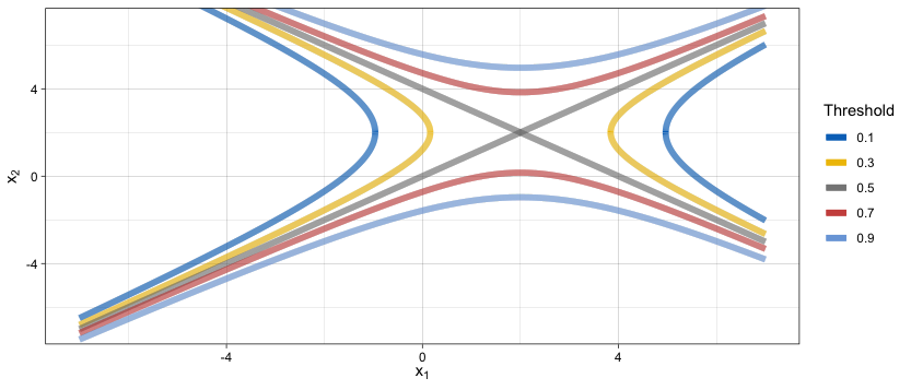
(a) a

(b) b

(c) c

Figure 3: (a) Optimal decision boundaries for target thresholds 0.1, 0.3, 0.5, 0.7, 0.9. Posterior median boundaries for (b) SB, and (c) TB.

As before, we investigate the performance of tailoring across a wide range of settings, by varying: (1) the sample size, (2) the prevalence of the outcome, (3) and the target threshold. Performance is evaluated in an independently sampled test set of size 2000. Figure 4 shows the difference in $NB$ between TB and SB. Tailoring performs similarly or better than standard regression across all target thresholds for prevalence scenarios 0.3 and 0.5. For 0.1 the two models are closely matched. A further comparison with a non-linear model, namely Bayesian Additive Regression Trees (BART) (Sparapani et al., 2021) is detailed in the supplementary material (Section S7). Briefly, TB demonstrated equivalent or better performance than BART at the clinically relevant lower disease prevalences of 0.1 and 0.3, indicating that the benefits offered by TB cannot be matched simply by switching to a non-linear modelling framework.

Figure 4: Difference in Net Benefit for samples sizes of 500, 1000, 5000, 10000 averaged over 20 repetitions. A positive difference means TB outperforms SB. Each grid corresponds to a different prevalence setting.

3.3 Simulation 3: Data contamination

Our third simulation scenario demonstrates the robustness of tailoring to data contamination i.e., the situation in which a fraction of the data have been mislabelled. The data generating model is a logistic regression with a large fraction of mislabelled datapoints. We simulate $d=2$ covariates and $n=1000$ datapoints. Figure 5 depicts a scenario with $10\%$ of datapoints mislabelled among those with high values of both covariates, i.e., among the upper right hand side of the data cloud. For each covariate, $1000$ values are independently drawn from a standard Gaussian distribution. Denoting the coefficient vector by $\bm{\beta}\in\mathbb{R}^{3}$ with values $\bm{\beta}=(0,2,3)$ (the first value corresponds to the intercept term) we simulate the outcome vector as $y\sim Bernoulli\Big{(}\frac{\exp\{{\mathbf{x}^{T}\bm{\beta}}\}}{1+\exp\{{\mathbf{x}^{T}\bm{\beta}}\}}\Big{)}$, where $\mathbf{x}=(1,x_{1},x_{2})^{T}$. We then corrupt the data with class 0 datapoints, i.e., we set $y:=0$ for $\psi n$ datapoints where $\psi$ is the fraction of contamination taking values $5\%,10\%,15\%,20\%$ and $30\%$. The covariates are generated from equivalent and independent normal distributions, specifically $x_{1},x_{2}\sim\mathcal{N}(1.5,0.5)$. This type of contamination framework has been popularised by Huber (1964, 1965) and used extensively to study the robustness of learning algorithms to adversarial attacks in general (Balakrishnan et al., 2017; Diakonikolas et al., 2018; Prasad et al., 2018; Osama et al., 2019) and medical applications (Paschali et al., 2018).

Figure 5: Single realisation from contaminated distribution with $10\%$ corrupted datapoints. Data ($n=1000$) with labels 0 and 1 are shown in blue and red, respectively. The corrupted data points are depicted with triangles on the upper right-hand corner of the data cloud. The lines corresponds to target thresholds 0.1, 0.5, and 0.9.

We derive the optimal $NB$ based on the true probability score in an independent non-contaminated test dataset of size $n=2000$. Figure 6 shows the results for various contamination fractions. For most fractions TB outperforms SB. As the contamination fraction gets larger the performance of both models degrades, but standard regression degrades at a faster rate. Tailoring can accommodate various degrees of contamination better than standard regression, while generally never resulting in poorer performance.

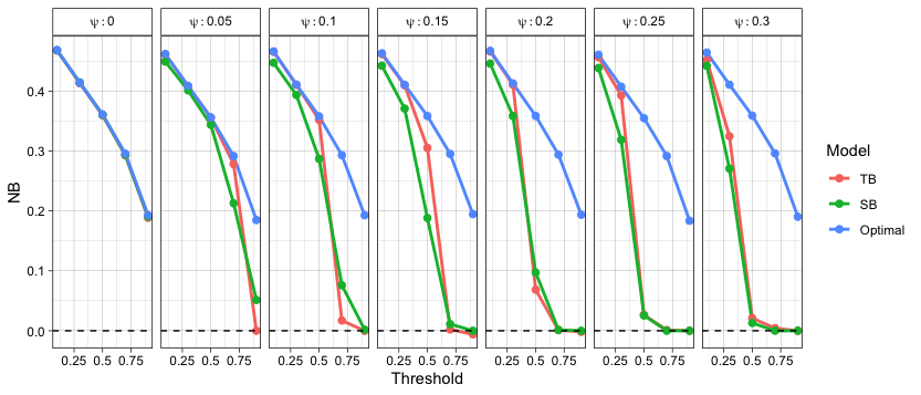
Figure 6: Net Benefit of tailoring (red) and standard regression (green) compared to optimal classification (blue) averaged over 20 repetitions. Each grid corresponds to different contamination fraction.

Note that under no contamination (i.e., $\psi=0$, first panel Figure 6) SB is an optimal classifier, since the optimal decision boundaries are parallel straight lines (Figure 5). However, for all other scenarios even a data corruption as small as 5% results in poor performance under SB for target thresholds $>0.5$. On the contrary, tailoring maintains stable performance and close to the optimal for $t<0.5$, for up to 15% of mislabelled datapoints.

4 Real data applications

We evaluate the performance of TB on three real-data applications involving a breast cancer prognostication task (Section 4.1), a cardiac surgery prognostication task (Section 4.2) and a breast cancer tumour classification task (supplementary material Section S8). Overall, our empirical results demonstrate the improvement in predictive performance when taking into consideration misclassification costs during model training.

4.1 Real data application 1: Breast cancer prognostication

Here, we apply the TB methodology to predict mortality after diagnosis with invasive breast cancer. The training data is based on 4718 oestrogen receptor positive subjects diagnosed in East Anglia, UK between 1999 and 2003. The outcome modelled is 10-year mortality. The covariates are age at diagnosis, tumor grade, tumor size, number of positive lymph nodes, presentation (screening vs. clinical), and type of adjuvant therapy (chemotherapy, endocrine therapy, or both). We use 20% of the data as design and the rest as development set (see Figure S1, supplementary material), repeating the design/development set split $m=5$ times. The entire train data is used to fit SB. Both models are evaluated in an independent test set consisting of 3810 subjects. Detailed information on the datasets can be found in Karapanagiotis et al. (2018).

An important part of the TB methodology is the choice of $t$. In breast cancer, accurate predictions are decisive because they guide treatment. In clinical practice, treatment is given if it is expected to reduce the predicted risk by at least some pre-specified magnitude. For instance, clinicians in the Cambridge Breast Unit (Addenbrooke’s Hospital, Cambridge, UK) currently use the absolute 10-year survival benefit from chemotherapy to guide decision making for adjuvant chemotherapy as follows: $<3\%$ no chemotherapy; $3\%-5\%$ chemotherapy discussed as a possible option; $>5\%$ chemotherapy recommended (Down et al., 2014). Following previous work (Karapanagiotis et al., 2018), we assume that chemotherapy reduces the 10-year risk of death by 22% (Peto et al., 2012). Then, a risk reduction between 3% and 5%, corresponds to target thresholds between 14% and 23%. Hence, we explore misclassification cost ratios corresponding to $t$ in the range between 0.1 and 0.5.

Figure 7 shows the difference in $NB$ between the two models averaged over the 5 splits. We see TB outperforms SB for most target thresholds, especially where decisions about adjuvant chemotherapy are made. Compared to SB, tailoring achieves up to 3.6 more true positives per 1000 patients (when $t=0.15$), which is equivalent to having 3.6 more true positives per 1000 patients for the same number of unnecessary treatments.

Figure 7: Difference in Net Benefit for various $t$ values evaluated on the test set. Error bars correspond to one standard error of the difference. That is, denoting the difference in Net Benefit $D^{i}=NB^{i}_{TB}-NB^{i}_{SB}$ with $i=1,\dots,m=5$ for each $t$ then the standard error of the difference is $SE_{D}=\sqrt{\frac{\sum(D^{i}-\bar{D})^{2}}{m(m-1)}}$, where $\bar{D}=\sum_{i}D^{i}/m$. This accounts for the fact that both models have been evaluated on the same data. The units on the y axis may be interpreted as the difference in benefit associated with one patient who would die without treatment and who receives therapy. The 0.14 to 0.23 shaded area on the x axis corresponds to 3%–5% absolute risk of death reduction with and without chemotherapy. These are the risk ranges where chemotherapy is discussed as a treatment option.

Next, we examine the effect of tailoring on the posterior distributions of the coefficients. As an exemplar, we use the posterior samples for the model corresponding to $t=0.15$ (Figure 8). We see that tailoring affects both the location and spread of the estimates compared to standard modelling. First, note the wider spread of tailoring compared to the standard models. Second, the tailored posteriors are centred on different values. The most extreme example is the coefficient for the number of nodes. Under tailoring it has a stronger positive association with the risk of death. To quantify the discrepancy between the posteriors of the two models table 1 shows estimates of the overlapping area between the posteriors for each covariate. These range from 3% to 70%. The relative shifts in magnitude of the effect sizes indicates different relative importance of the covariates in terms of their contribution to the predictions from the two models.

Figure 8: Marginal density plots of posterior parameters for $t=0.15$ for SB (blue) and TB (red).

Covariate	Posterior Overlap (%)
nodes	3.05
size	23.46
chemo	41.92
age	48.78
hormone	57.76
grade	62.66
screen	69.94

Table 1: Overlapping area of posterior distributions for each coefficient based Gaussian kernel density estimations (Pastore and Calcagnì, 2019).

4.2 Real data application 2: Cardiac surgery prognostication

For our second case study we investigate whether TB allows for better predictions, and consequently improved clinical decisions for patients undergoing aortic valve replacement (AVR). Cardiac patients with severe symptomatic aortic stenosis are considered for surgical AVR (SAVR). Given that SAVR is typically a high-risk procedure, transcatheter aortic valve implantation (TAVI) is recommended as a lower risk alternative but it is associated with higher rates of complications (Baumgartner et al., 2017). The European System for Cardiac Operative Risk Evaluation (EuroSCORE) is routinely used as a criterion to choose between SAVR and TAVI (Roques et al., 2003). EuroSCORE is an operative mortality risk prediction model which takes into account 17 covariates encompassing patient-related, cardiac and operation-related characteristics. It was first introduced by Nashef et al. (1999) and it has been updated in 2003 (Roques et al., 2003) and 2012 (Nashef et al., 2012). Published guidelines recommend TAVI over SAVR if a patient’s predicted mortality risk is above 10% (Baumgartner et al., 2017) or 20% (Vahanian et al., 2008). Here, we compare the performance of TB with EuroSCORE and SB given these target thresholds.

We use data ($n$ = 9031) from the National Adult Cardiac Surgery Audit (UK) collected between 2011 and 2018. We use 80% of the data for training and the rest for testing, repeating the train/test set split $m=5$ times. For this data a design set to estimate $\pi_{u}(\mathbf{x}_{i})$ is not necessary (see supplementary material Figure S1) but instead we use the predictions from EuroSCORE (Roques et al., 2003). We add an extra step of re-calibration to account for the population/time drift (Cox, 1958; Miller et al., 1993). Figure 9 presents the results. We see TB outperforms both EuroSCORE and SB when targeting the 0.1 threshold, and only EuroSCORE at $t=0.2$.

Figure 9: Difference in Net Benefit ($\Delta$NB) between TB and EuroSCORE (ES) (red), and between TB and SB (green) for various target thresholds evaluated on the test set. Error bars correspond to one standard error of the difference (see caption of Figure 7 for details).

We further investigate the effect of tailoring to individual parameters. Figure 10 shows the highest posterior density (HPD) regions for a subset of the covariates under SB and TB for $t=0.1$ and $0.2$. As in the previous case study, under tailoring the regions are generally wider and are centred on different values. For instance, compared to SB under both $t=0.1$ and 0.2 the posteriors of critical operative state and unstable angina are shifted towards the same direction (positive for critical operative state and negative for unstable angina). Contrast these with the posterior of emergency that compared to SB it is centred on more positive values under $t=0.1$ and more negative under $t=0.2$. On the contrary, extracardiac arteriopathy, recent myocardial infarct, and sex are centred on similar values across the three models. This once more exemplifies the change in the contribution of some covariates towards the predicted risks when taking into account misclassification costs.

Figure 10: Highest posterior density (HPD) regions for the parameters. Dots represent medians, and thick and thin lines represent 90 and the 95% of the HPD regions, respectively. The dashed vertical lines pass through the posterior median values of the SB parameters.

5 Discussion

In this work, we present Tailored Bayes, a framework to incorporate misclassification costs into Bayesian modelling. We demonstrate that our framework improves predictive performance compared to standard Bayesian modelling over a wide range of scenarios in which the costs of different classification errors are unbalanced.

The methodology relies solely on the construction of the datapoint-specific weights (see (7)). In particular, we need to specify $t$, the grid of $\lambda$ values for the CV, a model to estimate $\pi_{u}(\mathbf{x}_{i})$ and the weighting function, $h$. For some applications there may be a recommended target threshold, $t$. For instance, UK national guidelines recommend that clinicians use a risk prediction model (QRISK2; (Hippisley-Cox et al., 2008)) to determine whether to prescribe statins for primary prevention of cardiovascular disease (CVD) if a person’s CVD risk is 10% or more (NICE, 2016). When guidelines are not available, the specification of $t$ is inevitably subjective, since it reflects the decision maker’s preferences regarding the relative costs of different classification errors. In practice, eliciting these preferences may be challenging, despite the numerous techniques that have been proposed in the literature to help with this (e.g., Tsalatsanis et al. (2010); Hunink et al. (2014)). In such situations, we advocate fitting the model for a range of plausible $t$ values that reflect general decision preferences. For example, research in both mammographic (Schwartz et al., 2000) and colorectal cancer screening (Boone et al., 2013) has shown that healthcare professionals and patients alike greatly value gains in sensitivity over loss of specificity. For additional examples on setting $t$ see Vickers et al. (2016) and Wynants et al. (2019). Further examples in which benefits and costs associated with an intervention (as well as with patients’ preferences) are taken into account, are provided by Manchanda et al. (2016); Le et al. (2017); Watson et al. (2020).

We discuss the remaining elements for the construction of the weights in the supplementary material (Section S9). There we define the effective sample size for tailoring, $ESS_{t}$, and showcase how to use it to set the upper limit for the grid of $\lambda$ values. In addition, we show our framework is robust to miscalibration of $\pi_{u}(\mathbf{x}_{i})$ and the choice of $h$. The framework is therefore flexible, allowing many ways for the user to specify the weights.

In contrast to the work of Hand and Vinciotti (2003) our approach is framed within the Bayesian formalism. Consequently, the tailored posterior integrates the attractive features of Bayesian inference - such as flexible hierarchical modelling, the use of prior information and quantification of uncertainty - while also allowing for tailored inference. Quantification of uncertainty is critically important, especially in healthcare applications (Begoli et al., 2019; Kompa et al., 2021). Whilst two (or more) models can perform similarly in terms of aggregate metrics (e.g., area under ROC curve) they can provide very different individual (risk) predictions for the same patient (Pate et al., 2019; Li et al., 2020). This can ultimately lead to different decisions for the individual, with potential detrimental effects. Uncertainty quantification can mitigate this issue since it allows the clinician to abstain from utilising the model’s predictions. If there is high predictive uncertainty for an individual, the clinician can discount or even disregard the prediction.

To illustrate this point, we use the SB posterior from the breast cancer prognostication case study. The posterior predictive distributions for two patients are displayed in Figure 11. The average posterior risk for each patient is indicated by the vertical line at 34 and 35%, respectively. Based solely on these average estimates chemotherapy should be recommended as a treatment option to both patients (see Section 4.1). It is clear, however, that the predictive uncertainty for these two patients is quite different, as the distribution of risk for patient 1 is much more dispersed than the distribution for patient 2. One way to quantify the predictive uncertainty would be to calculate the standard deviation of these distributions, which are 6.9% and 2.8% for patient 1 and patient 2, respectively. Even though both estimates are centred at similar values the predictive uncertainty for patient 1 is more than two times higher than patient 2. Using this information, we could flag patient 1 as needing more information before making a clinical decision.

Figure 11: Predictive uncertainty for the risk of death in two patients. These posterior predictive distributions reflect the range of risks assigned to these patients, and the mean risk is shown as vertical lines. Despite the fact that both patients have similar mean risks, we may be more inclined to trust the predictions for patient 2 given the lower amount of uncertainty associated with that prediction.

A few related comments are in order. In this work we use vague Gaussian priors, but they could be replaced with other application-specific distribution choices. For instance, in the case of high-dimensional data another option could be the sparsity-inducing prior used by Bayesian lasso regression (Park and Casella, 2008). Furthermore, we can easily incorporate external information in a flexible manner, through $\pi_{u}(\mathbf{x})$, in addition to the prior on the coefficients. If a well-established model exists then it is natural to consider using it to improve the performance of an expanded model. We have implemented such an approach in Section 4.2. Cheng et al. (2019) propose several approaches for incorporating published summary associations as prior information when building risk models. A limitation of their approaches is the requirement for a parametric model, i.e., information on regression coefficients. Our method does not have any restriction on the form of $\pi_{u}(\mathbf{x})$, it can arise from a parametric or non-parametric model.

We note that we opted to use the same set of covariates, $\mathbf{x}$, to estimate both $\pi_{w_{i}}(\mathbf{x};\bm{\beta})$ and $\pi_{u}(\mathbf{x})$. This does not need to be the case. If available, we could instead use another set of covariates, say $\mathbf{Z}$ to estimate $\pi_{u}(\mathbf{z})$. The set $\mathbf{Z}$ could be a superset or a subset of $\mathbf{X}$ or the two sets could be completely disjoint. We also note that in this work we focus on linear logistic regression to showcase the methodology (linear refers to linear combinations of the covariates). This is because it is widely utilised and allows analytical and computational tractability. Nevertheless, we would stress that our framework is generic, and not restricted to linear logistic regression. It can accommodate a wide range of modelling frameworks, from linear to non-linear and from classical statistical approaches to state-of-the-art machine learning algorithms. As a result, future work could consider such extensions to non-linear models. Also, future work could consider the advantages of a joint estimation, i.e., both steps, stage 1 (estimation of weights) and stage 2 (estimation of weighted prediction probabilities) jointly. A further direction is the extension of the framework to high-dimensional settings.

To conclude, in response to recent calls for building clinically useful models (Chatterjee et al., 2016; Shah et al., 2019) we present an overarching Bayesian learning framework for binary classification where we take into account the different benefits/costs associated with correct and incorrect classifications. The framework requires the modellers to first think of how the model will be used and the consequences of decisions arising from its use - which we would argue should be a prerequisite for any modelling task. Instead of fitting a global, agnostic model and then deploying the result in a clinical setting we propose a Bayesian framework to build towards models tailored to the clinical application under consideration.

6 Software

The R code used for the experiments in this paper has been made available as an R package, TailoredBayes, on Github: https://github.com/solonkarapa/TailoredBayes

Supplementary Materials for Tailored Bayes: a risk modelling framework under unequal misclassification costs

Solon Karapanagiotis, Umberto Benedetto, Sach Mukherjee, Paul D. W. Kirk, Paul J. Newcombe

S1 Interpretation of the TB prior (and posterior)

Here we show the prior in TB can be interpreted as a regularizer on a per-datapoint influence/importance. First, we slightly modify notation and consider data $D_{i}=(X_{i},Y_{i})$ as a copy of a random variable $D=(X,Y)\in\mathbb{R}^{d}\times\{0,1\}$. Then, let $\mathcal{L}(D_{i}|\bm{\beta})$ be the standard likelihood contribution of datapoint $i$ ($i=1,\ldots,n)$. The TB posterior, up to a normalising constant, is

$$p(\bm{\beta}|D)\propto\prod_{i=1}^{n}\mathcal{L}(D_{i}|\bm{\beta})^{w_{i}}p(\bm{\beta}).$$ (S1)

Following Walker and Hjort (2001) we can view (S1) as combining the original likelihood function with a data-dependent prior that is divided by a portion of the likelihood. To see this, we first define the data-dependent prior as

$$\frac{p(\bm{\beta})}{\prod_{i=1}^{n}\mathcal{L}(D_{i}|\bm{\beta})^{1-w_{i}}}$$

which corresponds to

$$p(\bm{\beta}|D)\propto\prod_{i=1}^{n}\mathcal{L}(D_{i}|\bm{\beta})\frac{p(\bm{\beta})}{\prod_{i=1}^{n}\mathcal{L}(D_{i}|\bm{\beta})^{1-w_{i}}}=\prod_{i=1}^{n}\mathcal{L}(D_{i}|\bm{\beta})^{w_{i}}p(\bm{\beta}),$$

which is seen to coincide with (S1). This data-dependent downweighting of the prior reduces the weights of those parameter values that “track the data too closely” (Linero and Yang, 2018).

S2 Model inference and prediction

To sample from the TB posterior we use Markov Chain Monte Carlo (MCMC) (see Section S5 for details on the computational scheme). We obtain $S$ posterior samples $\{\bm{\beta}^{s}\}^{S}_{s=1}$, where $\bm{\beta}^{s}=(\beta^{s}_{1},\dots,\beta^{s}_{d+1})$. We use the posterior samples to approximate the predictive density for test data $\mathbf{x}_{*}$

$$\begin{split}p(\pi(\mathbf{x}_{*})\mid\mathbf{x}_{*},D)=\int p(\pi(\mathbf{x}_{*})\mid\mathbf{x}_{*},\bm{\beta})p(\bm{\beta}\mid D)d\bm{\beta}\\ \approx\frac{1}{S}\sum_{s=1}^{S}p(\pi(\mathbf{x}_{*})\mid\mathbf{x}_{*},\bm{\beta}^{s}).\end{split}$$ (S2)

To calculate point predictions we summarise (S2) by using the posterior predictive mean,

$$\begin{split}\hat{\pi}(\mathbf{x}_{*})=\int\pi(\mathbf{x}_{*})p(\pi(\mathbf{x}_{*})\mid\mathbf{x}_{*},D)d\pi(\mathbf{x}_{*}),\end{split}$$ (S3)

which is used as a plug-in into (5) in the main manuscript. We also use Bayesian inference for the estimation of $\pi_{u}(\mathbf{x})$ so $\pi(\mathbf{x}_{*})$ can be conceptually replaced by $\pi_{u}(\mathbf{x})$ in eq (S2) and (S3) with the caveat that they are estimated in different subsets of the data (see Section S4 for the data splitting stategy we are implementing).

S3 Cross-validation to choose $\lambda$

We use stratified $K$-fold cross-validation (CV) to choose $\lambda$ in (7) in the main manuscript. The stratification ensures the prevalence of the outcome is the same in each fold. In $K$-fold CV, the data is partitioned into $K$ subsets $D_{(k)}$, for $k=1,\dots,K$ and then the model is fit separately to each training set $D_{(-k)}$ thus yielding a posterior distribution $p(\bm{\beta}\mid D_{(-k)})$. When calculating the predictive performance of the model the data of the $k^{th}$ fold is used as test data. The predictive density for $\mathbf{x}_{*}$, if it is in subset $k$, is

$$\begin{split}p(\pi(\mathbf{x}_{*})\mid\mathbf{x}_{*},D_{(-k)})=\int p(\pi(\mathbf{x}_{*})\mid\mathbf{x}_{*},\bm{\beta})p(\bm{\beta}\mid D_{(-k)})d\bm{\beta}\\ \approx\frac{1}{S}\sum_{s=1}^{S}p(\pi(\mathbf{x}_{*})\mid\mathbf{x}_{*},\bm{\beta}^{s}).\end{split}$$ (S4)

and the posterior predictive expectation is $\hat{\pi}(\mathbf{x}_{*})=\int\pi(\mathbf{x}_{*})p(\pi(\mathbf{x}_{*})\mid\mathbf{x}_{*},D_{(-k)})d\pi(\mathbf{x}_{*})$ which is used as a plug-in into (5) in the main manuscript to calculate the $K$-fold CV estimate of NB in the $k^{th}$ fold, $\text{NB}_{(k)}$. We choose $\lambda$ as

$$\lambda^{*}=\operatorname*{arg\,max}_{\lambda}\frac{1}{K}\sum_{k=1}^{K}\text{NB}_{(k)}.$$

We use $K=5$ for the all analysis. In practice, we have seen the results are insensitive to the choice of $K$.

S4 Data splitting strategy

To avoid overfitting due to the estimation of both $\pi_{u}(\mathbf{x}_{i})$ and $\pi_{w_{i}}(\mathbf{x}_{i};\bm{\beta})$ from the same dataset we use the following data splitting process (Figure S1 and Pseudo-Code 1). First, the data is split into training and testing sets. This step is avoided if we already have an independent test set (Section 4.1 main manuscript) or if data is simulated (Section 3 main manuscript). The train set is subsequently split again into design (20%) and development (80%). The design part is used to estimate $\pi_{u}(\mathbf{x}_{i})$. The development part is used to choose $\lambda$ (with 5-fold stratified CV, see Section S3 for details). After choosing a $\lambda$ value the model is fit to the entire development part, and it is with respect to the posterior from this final fit credible intervals are generated in the analyses. Finally, the test set is used to validate the performance of the model. We opted for this three-way splitting strategy, design-development-test set, because we have large datasets available but any other method such as leave-one-out, (nested) cross-validation, or bootstrap methods could be used.

Figure S1: The data splitting strategy. The dataset, $D$, is split into train ($D_{train})$ and test ($D_{test}$) sets. The train set is subsequently split again into design ($D_{design}$) (20%) and development ($D_{develop}$) (80%). The design part is used to estimate $\hat{\pi}_{u}(\mathbf{x}_{i})$. The development part is used to choose $\lambda^{*}$ (5-fold CV, see Section S3 for details). After choosing a $\lambda^{*}$ value the model is fit to the entire development part, obtaining the posterior, $p(\bm{\beta}|D_{develop})$. Finally, the test set is used to create predictions, $\hat{\pi}(\mathbf{x}_{*})$ (this is the posterior predictive mean defined in Section S2.)

input: $D$: dataset, $K$: number of folds for the cross-validation, $\lambda$: tuning parameter, Model_u: model to estimate $\pi_{u}(\mathbf{x}_{i})$, Model_w: model to estimate $\pi_{w_{i}}(\mathbf{x}_{i};\bm{\beta})$

procedure TB($D,K,\lambda,\text{Model}_{u},\text{Model}_{w}$)

1. $D_{design}$, $D_{develop}$, $D_{test}$ $\leftarrow$ $D$ $\triangleright$ randomly split $D$ into design, development and test sets

2. $f_{u}$ $\leftarrow$ Model${}_{u}(D_{design})$ $\triangleright$ train a model on $D_{design}$ to estimate a function $f_{u}$

3. $\hat{\pi}_{u}(\mathbf{x}_{i})\leftarrow f_{u}(\mathbf{x}_{i})$ $\triangleright$ apply the function $f_{u}$ to $\mathbf{x}_{i}$ where $i\in D_{develop}$ to obtain $\hat{\pi}_{u}(\mathbf{x}_{i})$

4. $\lambda^{*}\leftarrow\text{CV}(D_{develop},K,\lambda$) $\triangleright$ use cross-validation to obtain $\lambda^{*}$

5. $f\leftarrow\text{Model}_{w}(D_{develop},\lambda^{*})$ $\triangleright$ train a model on $D_{develop}$ to estimate a function $f$

6. $\hat{\pi}(\mathbf{x}_{*})\leftarrow f(\mathbf{x}_{*})$ $\triangleright$ apply the function $f$ to $\mathbf{x}_{*}\in D_{test}$ to obtain $\hat{\pi}(\mathbf{x}_{*})$

7. end procedure

output: $\hat{\pi}(\mathbf{x}_{*})$                 $\triangleright$ the posterior predictive mean. Additionally, the posterior distribution of $f$ can be returned

Pseudo-code 1 The TB algorithm.

S5 Computational scheme

For all analysis in this report we use MCMC which has become a very important computational tool in Bayesian statistics since it allows for Monte Carlo approximation of complex posterior distributions where analytical or numerical integration techniques are not applicable. The Markov chain is constructed using random walk Metropolis-Hastings updates (Brooks et al., 2011). We give a brief overview of the algorithm.

The target distribution is $p(\bm{\beta}|D)$ (see (10) main manuscript). The sampling scheme starts at an initial set of parameter values, denote these $\bm{\beta}^{0}$. To sample the next set of parameters, which we denote $\bm{\beta}^{1}$, we propose moving from the current state to another set of parameter values, $\bm{\beta}^{new}$, by using a proposal function $q(\bm{\beta}^{new}|\bm{\beta})$. We then accept these proposed values as the next sample with probability equal to the Metropolis-Hastings ratio:

$$\text{MHR}(\bm{\beta},\bm{\beta}^{new})=\frac{L(D|\bm{\beta}^{new})p(\bm{\beta}^{new})}{L(D|\bm{\beta})p(\bm{\beta})}\times\frac{q(\bm{\beta}|\bm{\beta}^{new})}{q(\bm{\beta}^{new}|\bm{\beta})},$$ (S5)

where $L(D|\bm{\beta})$ is the tailored likelihood and $p(\bm{\beta})$ the prior, given in Sections 2.4 and 2.5 of the main manuscript. The proposed move is accepted with probability

$$\alpha(\bm{\beta},\bm{\beta}^{new})=min(1,\text{MHR}(\bm{\beta},\bm{\beta}^{new})).$$

If this new set of values is accepted, the proposed set is accepted as $\bm{\beta}^{1}$; otherwise, the sample value remains equal to the current sample value, i.e., $\bm{\beta}^{1}=\bm{\beta}^{0}$. The proposal function is Gaussian, i.e., $q\sim\mathcal{N}(\bm{\beta},\bm{I}sd)$ where $sd$ is chosen to yield an acceptance rate $\approx 0.24$ (Brooks et al., 2011). In the current version of the algorithm all parameters are updated jointly.

S6 Supplementary Figures

Figure S2: Single realisation from model in Section 3.1 with $q=0.1$ corresponding to prevalence of around 0.15. Optimal decision boundaries (black lines) for target thresholds 0.1, 0.3, 0.5, 0.7, 0.9. Posterior mean boundaries for SB (grey) and TB (yellow) when targeting the 0.5 boundary. Shaded regions represent 90% highest predictive density (HPD) regions.

S7 Comparison with BART

Given the non-linear decision boundaries of the simulation scenario in Section 3.2, we further compare TB with a standard non-linear Bayesian model. We use logistic Bayesian Additive Regression Trees (BART) as implemented in the BART package version 2.9 (lbart() function) (Sparapani et al., 2021).

Figure S3 shows the difference in NB between TB and BART. Under the 0.5 prevalence scenario BART performs better than TB except at $t=0.9$. On the other hand, TB performs better or no worse than BART under prevalence scenarios 0.1 and 0.3. This is noteworthy as these prevalence scenarios are common in medical applications. Together with the results from Figure 4 (main manuscript), we conclude that for this simulation scenario, TB, albeit implemented as a linear model, mitigates some of the advantages of a non-linear one, such as BART. Note that an additional comparison of interest would be BART with a tailored BART implementation. We leave this for future work.

Figure S3: Difference in Net Benefit for samples sizes of 500, 1000, 5000, 10000 averaged over 20 repetitions. A positive difference means TB outperforms BART. Each grid corresponds to a different prevalence setting.

S8 Real data application 3: Breast cancer tumour classification

For our third case study we use the Wisconsin breast cancer tumour dataset from the UCI repository (Dua and Graff, 2017). The dataset consists of $n=699$ points, with covariates $\mathbf{x}\in\mathbb{R}^{9}$, which describe characteristics of the cell nuclei present in digitized images of a breast mass, and labels $y\in\{0,1\}$. The class labels 0 and 1 correspond to ‘benign’ and ‘malignant’ cancers, respectively. To validate the results of the simulation in Section 3.3 in the main manuscript we artificially contaminate the dataset. More precisely, we use $70\%$ of the data for training, which is corrupted by flipping the labels of 49 class 1 datapoints to 0 ($10\%$ contamination). In clinical practice, such data contamination may arise due to the manual nature of breast cancer detection and classification. Breast cancer detection is commonly performed through medical imaging modalities by one or more experts (usually pathologists) (Murtaza et al., 2019). The procedure is time-consuming and dependent on the professional experience and domain knowledge of the pathologists, thus making it prone to errors. This is highlighted by the significant inter- and intra-variability between pathologists (Warfield et al., 2008; Li et al., 2009; Hong et al., 2012). We use 20% of the training data as design and the rest as development set. We assume that missing a malignant cancer is more severe than misdiagnosing a benign as malignant, and so we focus on target thresholds $t<0.5$, which correspond to a larger weight placed on false negatives vs false positives. Figure S4 presents the difference in NB for various $t$ values over 5 splits of the training data into design and development. We see tailoring outperforms standard regression for most target thresholds.

Figure S4: Difference in Net Benefit for various $t$ values evaluated on the test set. Error bars correspond to one standard error of the difference (see caption of Figure 7 main manuscript for details).

We further investigate the effect of tailoring on individual parameter values. Figure S5 shows the highest posterior density (HPD) regions under SB and TB for $t=0.3$ and $0.5$. As in the other case studies, under tailoring the regions are generally wider and are centred on different values. For instance, under $t=0.3$ all posteriors are shifted towards more positives values. The only two exceptions are the coefficients of clump thickness, cell shape and mitosis which are pulled towards zero. Similar conclusions, but less pronounced are seen under $t=0.5$. This again indicates that the relative importance of different features changes when using our tailored modelling approach.

Figure S5: Highest posterior density (HPD) regions for the parameters. Dots represent medians, and thick and thin lines represent 90 and the 95% of the HPD regions, respectively. The dashed vertical lines pass through the posterior median values of the SB parameters.

S9 Discussion Topics and Implementation Considerations

The method presented in this paper relies on the construction of the datapoint-specific weights (see (7) in the main manuscript). Here we discuss each element in turn.

S9.1 On choosing $\lambda$

We have opted to use cross-validation to choose $\lambda$. An open question is how to choose the range of $\lambda$ values to consider. Our proposal is to consider values of the form $\lambda\in\{0,\dots,m\}$. When $\lambda=0$, the model reduces to standard logistic regression, a sensible choice for the lower limit. To choose the upper limit, $m$, note that as $\lambda$ increases the rate with which the datapoints are downweighted increases exponentially (Figure S6). This in turn decreases the effective number of datapoints that are used when training the model. We call this the effective sample size for tailoring, $ESS_{T}$. Formally, we define $ESS_{T}$ as

$$ESS_{T}=\sum_{i=1}^{n}w_{i}.$$

Under standard modelling, $ESS_{T}=n$, since $w_{i}=1$, $\forall i$. Under tailoring $ESS_{T}\leq n$, which is why tailoring results in wider posteriors. This is demonstrated in Figure 1 of the main manuscript. In addition, Figure S7 shows the precision (as measured by the width) of the HPD credible intervals produced by each model under the simulation setting in Section 3.2 of the main manuscript. The figure suggests that the width of the credible intervals increases under tailoring compared to standard modelling. This is expected due to the downweighting of the likelihood contributions.

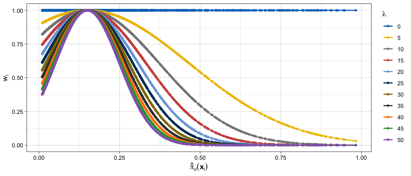
Figure S6: Distribution of weights, $w_{i}$, against $\hat{\pi}_{u}(\mathbf{x}_{i})$ for breast cancer prognostication case study (Section 4.1 main manuscript) for $t=0.15$

As a result, we can use the $ESS_{T}$ as a guide to choose $m$. Figure S8 shows $\frac{ESS_{T}}{n}$ for various $\lambda$ values and target thresholds for the breast cancer prognostication case study (Section 4.1 main manuscript). Based on a target threshold we can choose $m$ so the $ESS_{T}$ does not drop below a pre-specified threshold. Importantly, this plot can be produced before fitting the model since we only need estimates of $\pi_{u}(\mathbf{x}_{i})$.

Figure S7: 90% HPD Interval width for each parameter as a function of the model.

Figure S8: $\frac{ESS_{T}}{n}$ for various $\lambda$ values per target threshold.

In a similar fashion, we can have an indication whether TB will outperform SB before fitting the model. This can be achieved by plotting NB as $\lambda$ increases (Figure S9). If NB remains stable or decreases as $\lambda$ increases (Figure S9, $t=0.5$ orange points) then TB will probably not offer any performance improvement compared to SB (see Figure 7 main text, $t=0.5$). This is because, as discussed above, when $\lambda=0$ TB reduces to SB (i.e., all weights are equal to one).

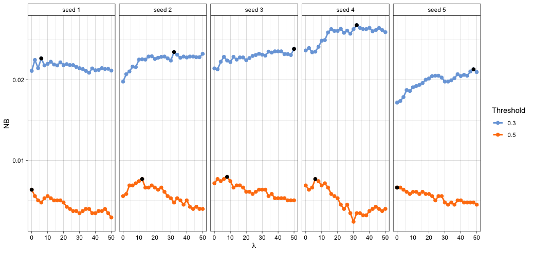
Figure S9: Average 5-fold CV estimate of Net Benefit (NB) for the breast cancer prognostication dataset. Black points correspond to the chosen lambda values, $\lambda^{*}$ (defined in Section S3).

S9.2 On calibration

Accurate estimation of $\pi_{u}(\mathbf{x}_{i})$ at the first step of our framework is important for the construction of the weights. Ideally, we would like the estimated probabilities, $\hat{\pi}_{u}(\mathbf{x}_{i})$ to be well calibrated. Calibration refers to the degree of agreement between observed and estimated probabilities. Probabilities are well calibrated if, for every 100 patients given a risk of x%, close to x have the event.

We use the breast cancer prognostication case study (Section 4.1 main manuscript) to investigate the effect of miscalibration on the model performance. First, we assess the calibration of $\hat{\pi}_{u}(\mathbf{x}_{i})$. Figure S10a presents a graphical evaluation of calibration. It is based on loess-based smoothing method (Austin and Steyerberg, 2014) where the estimated (i.e., $\hat{\pi}_{u}(\mathbf{x}_{i})$) and observed probabilities (from the development data) are plotted against each other; good models are close to the 45-degree line. We see the probabilities are well calibrated for the lower risks, and tend to be underestimated for the higher risks. To explore sensitivity of the tailored model to the accuracy of the step 1 probabilities, we deliberately perturbed $\hat{\pi}_{u}(\mathbf{x}_{i})$ generating four miscalibration types: (1) overestimation; (2) underestimation, when probabilities are systematically overestimated or underestimated, respectively; (3) overfitting, when small probabilities are underestimated whereas large ones are overestimated; (4) underfitting, when small probabilities are overestimated whereas large ones are underestimated. We further allowed for two degrees of miscalibration (mild and severe) for each type giving us a total of eight scenarios (Figure S10b).

(a) a

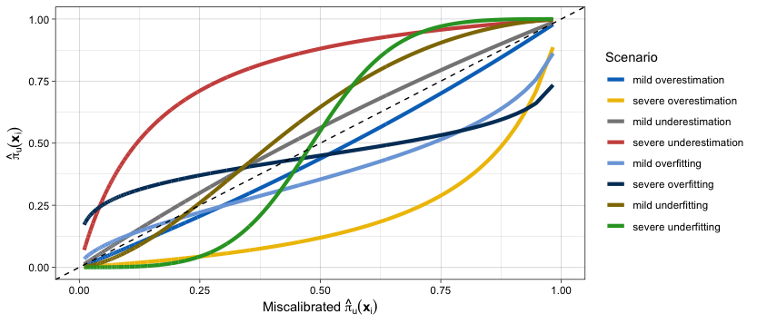
(b) b

Figure S10: (a) Calibration plot of $\hat{\pi}_{u}(\mathbf{x}_{i})$ on the train data using loess smoother. The 45-degree line represents the perfect calibration. (b) Illustrations of different miscalibration scenarios. The y axis shows $\hat{\pi}_{u}(\mathbf{x}_{i})$ and the x axis the miscalibrated $\hat{\pi}(\mathbf{x}_{i})$ used in model fitting.

Figure S11 shows the difference in NB between the original tailored (calibrated) model and the tailored miscalibrated ones for the different scenarios. Comparing across miscalibration types we see that the decline in performance depends on the type of miscalibration, with overfitting and underfittng more robust than over- and underestimation. Comparing within each type we note a drop in performance from mild to severe degrees, especially for over- and underestimation.

These results show that the model performance (in terms of NB) depends on the type of miscalibration and is robust to mild miscalibration. In practice, the calibration of the estimated probabilities can be readily evaluated graphically as done here or using statistical tests (Austin and Steyerberg, 2014). If the results show poor calibration we recommend re-calibrating $\hat{\pi}_{u}(\mathbf{x}_{i})$ before calculating the datapoint-specific weights (Steyerberg et al., 2004; Janssen et al., 2008).

Figure S11: Difference in NB, $\Delta$NB (on the test set) between original, calibrated TB and miscalibrated TB under different scenarios. A positive difference means the calibrated TB outperforms the miscalibrated one.

S9.3 On the weighting function

In Section 2.3 of the main manuscript we defined the weights using the squared distance function, $h$. Here we investigate the sensitivity of the framework to the choice of the distance function. We choose the family of $\epsilon$-insensitive functions (Vapnik, 1998), which is defined as

$$h(\pi_{u}(\mathbf{x}),t)=|\pi_{u}(\mathbf{x})-t|_{\epsilon}$$

where we denote

$$|\pi_{u}(\mathbf{x})-t|_{\epsilon}=\begin{cases}0&\text{if }|\pi_{u}(\mathbf{x})-t|\leq\epsilon\\ |\pi_{u}(\mathbf{x})-t|-\epsilon&\text{otherwise }\end{cases}$$ (S6)

The $\epsilon$-insensitivity arises from the fact that the function value is equal to 0 if the discrepancy between the predicted probability $\pi_{u}(\mathbf{x})$ and the target threshold $t$ is less than $\epsilon$. In other words, we do not care about the distance as long as it is less than $\epsilon$, but will not accept any deviation larger than this. As a result, observations with predicted probability within $\epsilon$ of the target threshold will not be downweighted. For $\epsilon=0$ we recover the absolute distance, which is the objective function in median regression (Bassett Jr and Koenker, 1978). Both the squared distance and the family of $\epsilon$-insensitive functions are symmetric, i.e., they downweight equally observations based only on their distance from the target threshold, not taking into account the direction. This is a reasonable requirement for our weighting function. Figure S12 presents the results for various $\epsilon$ values for the breast cancer case study (Section 4.1 main manuscript). The conclusions are qualitatively unchanged when compared within different $\epsilon$ values and between $\epsilon$-insensitive functions and the squared distance (first panel in Figure S12). Hence, we conclude that for this dataset the results are also robust to the choice of the weighting function.

Figure S12: Difference in NB (breast cancer prognostication case study) between TB and SB under the squared distance and $\epsilon$-insensitive functions for various $\epsilon$ values. Note the first panel corresponds to Figure 7 in the main manuscript.

References

- Austin and Steyerberg (2014) P. C. Austin and E. W. Steyerberg. Graphical assessment of internal and external calibration of logistic regression models by using loess smoothers. Statistics in Medicine, 33(3):517–535, 2014.
- Baker et al. (2009) S. G. Baker, N. R. Cook, A. Vickers, and B. S. Kramer. Using relative utility curves to evaluate risk prediction. Journal of the Royal Statistical Society: Series A, 172(4):729–748, 2009.
- Balakrishnan et al. (2017) S. Balakrishnan, S. S. Du, J. Li, and A. Singh. Computationally efficient robust sparse estimation in high dimensions. In Conference on Learning Theory, pages 169–212, 2017.
- Bartlett et al. (2006) P. L. Bartlett, M. I. Jordan, and J. D. McAuliffe. Convexity, classification, and risk bounds. Journal of the American Statistical Association, 101(473):138–156, 2006.
- Bassett Jr and Koenker (1978) G. Bassett Jr and R. Koenker. Asymptotic theory of least absolute error regression. Journal of the American Statistical Association, 73(363):618–622, 1978.
- Baumgartner et al. (2017) H. Baumgartner, V. Falk, J. J. Bax, M. De Bonis, C. Hamm, P. J. Holm, B. Iung, P. Lancellotti, E. Lansac, D. Rodriguez Munoz, et al. 2017 esc/eacts guidelines for the management of valvular heart disease. European Heart Journal, 38(36):2739–2791, 2017.
- Begoli et al. (2019) E. Begoli, T. Bhattacharya, and D. Kusnezov. The need for uncertainty quantification in machine-assisted medical decision making. Nature Machine Intelligence, 1(1):20–23, 2019.
- Bernardo and Smith (2009) J. M. Bernardo and A. F. Smith. Bayesian theory, volume 405. John Wiley & Sons, 2009.
- Bissiri et al. (2016) P. G. Bissiri, C. Holmes, and S. G. Walker. A general framework for updating belief distributions. Journal of the Royal Statistical Society: Series B, 78(5):1103–1130, 2016.
- Boone et al. (2013) D. Boone, S. Mallett, S. Zhu, G. L. Yao, N. Bell, A. Ghanouni, C. von Wagner, S. A. Taylor, D. G. Altman, R. Lilford, et al. Patients’ healthcare professionals’ values regarding true-& false-positive diagnosis when colorectal cancer screening by CT colonography: discrete choice experiment. PLOS ONE, 8(12), 2013.
- Brooks et al. (2011) S. Brooks, A. Gelman, G. Jones, and X.-L. Meng. Handbook of Markov Chain Monte Carlo. CRC press, 2011.
- Chatterjee et al. (2016) N. Chatterjee, J. Shi, and M. García-Closas. Developing and evaluating polygenic risk prediction models for stratified disease prevention. Nature Reviews Genetics, 17(7):392, 2016.
- Cheng et al. (2019) W. Cheng, J. M. Taylor, T. Gu, S. A. Tomlins, and B. Mukherjee. Informing a risk prediction model for binary outcomes with external coefficient information. Journal of the Royal Statistical Society: Series C, 68(1):121–139, 2019.
- Childress and Beauchamp (2001) J. F. Childress and T. L. Beauchamp. Principles of biomedical ethics. Oxford University Press New York, 2001.
- Cox (1958) D. R. Cox. Two further applications of a model for binary regression. Biometrika, 45(3/4):562–565, 1958.
- Diakonikolas et al. (2018) I. Diakonikolas, G. Kamath, D. M. Kane, J. Li, J. Steinhardt, and A. Stewart. Sever: A robust meta-algorithm for stochastic optimization. arXiv preprint arXiv:1803.02815, 2018.
- Down et al. (2014) S. K. Down, O. Lucas, J. R. Benson, and G. C. Wishart. Effect of predict on chemotherapy/trastuzumab recommendations in her2-positive patients with early-stage breast cancer. Oncology letters, 8(6):2757–2761, 2014.
- Dua and Graff (2017) D. Dua and C. Graff. UCI machine learning repository, 2017. URL http://archive.ics.uci.edu/ml.
- Duda et al. (2012) R. O. Duda, P. E. Hart, and D. G. Stork. Pattern classification. John Wiley & Sons, 2012.
- Elkan (2001) C. Elkan. The foundations of cost-sensitive learning. In Proceedings of the 17th International Joint Conference on Artificial Intelligence - Volume 2, IJCAI’01, page 973–978, San Francisco, CA, USA, 2001. Morgan Kaufmann Publishers Inc. ISBN 1558608125.
- Freedman (1987) B. Freedman. Equipoise and the ethics of clinical research. New England Journal of Medicine, 317(3):141–145, 1987.
- Friedman et al. (2000) J. Friedman, T. Hastie, R. Tibshirani, et al. Additive logistic regression: a statistical view of boosting (with discussion and a rejoinder by the authors). The Annals of Statistics, 28(2):337–407, 2000.
- Hand and Vinciotti (2003) D. J. Hand and V. Vinciotti. Local versus global models for classification problems: Fitting models where it matters. The American Statistician, 57(2):124–131, 2003.
- Hippisley-Cox et al. (2008) J. Hippisley-Cox, C. Coupland, Y. Vinogradova, J. Robson, R. Minhas, A. Sheikh, and P. Brindle. Predicting cardiovascular risk in england and wales: prospective derivation and validation of qrisk2. Bmj, 336(7659):1475–1482, 2008.
- Hong et al. (2012) T. S. Hong, W. A. Tomé, and P. M. Harari. Heterogeneity in head and neck IMRT target design and clinical practice. Radiotherapy and Oncology, 103(1):92–98, 2012.
- Huber (1964) P. J. Huber. Robust estimation of a location parameter. Ann. Math. Statist., 35(1):73–101, 1964. doi: 10.1214/aoms/1177703732. URL https://doi.org/10.1214/aoms/1177703732.
- Huber (1965) P. J. Huber. A robust version of the probability ratio test. Ann. Math. Statist., 36(6):1753–1758, 1965. doi: 10.1214/aoms/1177699803. URL https://doi.org/10.1214/aoms/1177699803.
- Hunink et al. (2014) M. M. Hunink, M. C. Weinstein, E. Wittenberg, M. F. Drummond, J. S. Pliskin, J. B. Wong, and P. P. Glasziou. Decision making in health and medicine: integrating evidence and values. Cambridge University Press, 2014.
- Janssen et al. (2008) K. Janssen, K. Moons, C. Kalkman, D. Grobbee, and Y. Vergouwe. Updating methods improved the performance of a clinical prediction model in new patients. Journal of Clinical Epidemiology, 61(1):76–86, 2008.
- Karapanagiotis et al. (2018) S. Karapanagiotis, P. D. Pharoah, C. H. Jackson, and P. J. Newcombe. Development and external validation of prediction models for 10-year survival of invasive breast cancer. comparison with predict and cancermath. Clinical Cancer Research, 24(9):2110–2115, 2018.
- Kompa et al. (2021) B. Kompa, J. Snoek, and A. L. Beam. Second opinion needed: communicating uncertainty in medical machine learning. NPJ Digital Medicine, 4(1):1–6, 2021.
- Kukar et al. (1998) M. Kukar, I. Kononenko, et al. Cost-sensitive learning with neural networks. In ECAI, volume 98, pages 445–449, 1998.
- Le et al. (2017) P. Le, K. Martinez, M. Pappas, and M. Rothberg. A decision model to estimate a risk threshold for venous thromboembolism prophylaxis in hospitalized medical patients. Journal of Thrombosis and Haemostasis, 15(6):1132–1141, 2017.
- Li et al. (2009) X. A. Li, A. Tai, D. W. Arthur, T. A. Buchholz, S. Macdonald, L. B. Marks, J. M. Moran, L. J. Pierce, R. Rabinovitch, A. Taghian, et al. Variability of target and normal structure delineation for breast cancer radiotherapy: an RTOG multi-institutional and multiobserver study. International Journal of Radiation Oncology* Biology* Physics, 73(3):944–951, 2009.
- Li et al. (2020) Y. Li, M. Sperrin, D. M. Ashcroft, and T. P. van Staa. Consistency of variety of machine learning and statistical models in predicting clinical risks of individual patients: longitudinal cohort study using cardiovascular disease as exemplar. BMJ, 371, 2020.
- Linero and Yang (2018) A. R. Linero and Y. Yang. Bayesian regression tree ensembles that adapt to smoothness and sparsity. Journal of the Royal Statistical Society: Series B, 80(5):1087–1110, 2018.
- Ling et al. (2004) C. X. Ling, Q. Yang, J. Wang, and S. Zhang. Decision trees with minimal costs. In Proceedings of the twenty-first international conference on Machine learning, page 69, 2004.
- Manchanda et al. (2016) R. Manchanda, R. Legood, A. C. Antoniou, V. S. Gordeev, and U. Menon. Specifying the ovarian cancer risk threshold of ‘premenopausal risk-reducing salpingo-oophorectomy’for ovarian cancer prevention: a cost-effectiveness analysis. Journal of Medical Genetics, 53(9):591–599, 2016.
- Margineantu and Dietterich (2003) D. Margineantu and T. Dietterich. A wrapper method for cost-sensitive learning via stratification, 2003. [Online; cited Decemeber 2019] Available at: :http://citeseerx.ist.psu.edu/viewdoc/summary?doi=10.1.1.27.1102.
- Masnadi-Shirazi and Vasconcelos (2010) H. Masnadi-Shirazi and N. Vasconcelos. Risk minimization, probability elicitation, and cost-sensitive svms. In ICML, pages 759–766, 2010.
- Miller et al. (1993) M. E. Miller, C. D. Langefeld, W. M. Tierney, S. L. Hui, and C. J. McDonald. Validation of probabilistic predictions. Medical Decision Making, 13(1):49–57, 1993.
- Murtaza et al. (2019) G. Murtaza, L. Shuib, A. W. A. Wahab, G. Mujtaba, H. F. Nweke, M. A. Al-garadi, F. Zulfiqar, G. Raza, and N. A. Azmi. Deep learning-based breast cancer classification through medical imaging modalities: state of the art and research challenges. Artificial Intelligence Review, pages 1–66, 2019.
- Nashef et al. (1999) S. A. Nashef, F. Roques, P. Michel, E. Gauducheau, S. Lemeshow, R. Salamon, and E. S. Group. European system for cardiac operative risk evaluation (Euro SCORE). European Journal of Cardio-Thoracic Surgery, 16(1):9–13, 1999.
- Nashef et al. (2012) S. A. Nashef, F. Roques, L. D. Sharples, J. Nilsson, C. Smith, A. R. Goldstone, and U. Lockowandt. Euroscore II. European journal of cardio-thoracic surgery, 41(4):734–745, 2012.
- NICE (2016) NICE. Cardiovascular disease: risk assessment and reduction, including lipid modification. 2016. [Online; cited Decemeber 2019] Available at: https://www.nice.org.uk/guidance/cg181/chapter/1-recommendations.
- Osama et al. (2019) M. Osama, D. Zachariah, and P. Stoica. Robust risk minimization for statistical learning. arXiv preprint arXiv:1910.01544, 2019.
- Park and Casella (2008) T. Park and G. Casella. The Bayesian Lasso. Journal of the American Statistical Association, 103(482):681–686, 2008.
- Paschali et al. (2018) M. Paschali, S. Conjeti, F. Navarro, and N. Navab. Generalizability vs. robustness: adversarial examples for medical imaging. arXiv preprint arXiv:1804.00504, 2018.
- Pastore and Calcagnì (2019) M. Pastore and A. Calcagnì. Measuring distribution similarities between samples: A distribution-free overlapping index. Frontiers in Psychology, 10:1089, 2019.
- Pate et al. (2019) A. Pate, R. Emsley, D. M. Ashcroft, B. Brown, and T. van Staa. The uncertainty with using risk prediction models for individual decision making: an exemplar cohort study examining the prediction of cardiovascular disease in english primary care. BMC medicine, 17(1):1–16, 2019.
- Pauker and Kassirer (1975) S. G. Pauker and J. P. Kassirer. Therapeutic decision making: a cost-benefit analysis. New England Journal of Medicine, 293(5):229–234, 1975.
- Pauker and Kassirer (1980) S. G. Pauker and J. P. Kassirer. The threshold approach to clinical decision making. New England Journal of Medicine, 302(20):1109–1117, 1980.
- Peto et al. (2012) R. Peto, C. Davies, J. Godwin, R. Gray, H. Pan, M. Clarke, D. Cutter, S. Darby, P. McGale, C. Taylor, et al. Comparisons between different polychemotherapy regimens for early breast cancer: meta-analyses of long-term outcome among 100,000 women in 123 randomised trials. Lancet, 379(9814):432–444, 2012.
- Prasad et al. (2018) A. Prasad, A. S. Suggala, S. Balakrishnan, and P. Ravikumar. Robust estimation via robust gradient estimation. arXiv preprint arXiv:1802.06485, 2018.
- Roques et al. (2003) F. Roques, P. Michel, A. Goldstone, and S. Nashef. The logistic EuroSCORE. European Heart Journal, 24(9):882–883, 2003.
- Schwartz et al. (2000) L. M. Schwartz, S. Woloshin, H. C. Sox, B. Fischhoff, and H. G. Welch. US women’s attitudes to false positive mammography results and detection of ductal carcinoma in situ: cross sectional survey. BMJ, 320(7250):1635–1640, 2000.
- Shah et al. (2019) N. H. Shah, A. Milstein, and S. C. Bagley. Making machine learning models clinically useful. JAMA, 322(14):1351–1352, 2019.
- Sparapani et al. (2021) R. Sparapani, C. Spanbauer, and R. McCulloch. Nonparametric machine learning and efficient computation with Bayesian additive regression trees: The BART R package. Journal of Statistical Software, 97(1):1–66, 2021. doi: 10.18637/jss.v097.i01.
- Steinwart (2005) I. Steinwart. Consistency of support vector machines and other regularized kernel classifiers. IEEE Transactions on Information Theory, 51(1):128–142, 2005.
- Steyerberg et al. (2004) E. W. Steyerberg, G. J. Borsboom, H. C. van Houwelingen, M. J. Eijkemans, and J. D. F. Habbema. Validation and updating of predictive logistic regression models: a study on sample size and shrinkage. Statistics in Medicine, 23(16):2567–2586, 2004.
- Ting (1998) K. M. Ting. Inducing cost-sensitive trees via instance weighting. In Principles of Data Mining and Knowledge Discovery, pages 139–147. Springer Berlin Heidelberg, 1998.
- Tsalatsanis et al. (2010) A. Tsalatsanis, I. Hozo, A. Vickers, and B. Djulbegovic. A regret theory approach to decision curve analysis: a novel method for eliciting decision makers’ preferences and decision-making. BMC Medical Informatics and Decision Making, 10(1):51, 2010.
- Turner (2013) J. R. Turner. Encyclopedia of Behavioral Medicine, chapter Principle of Equipoise, pages 1537–1538. Springer New York, 2013.
- Vahanian et al. (2008) A. Vahanian, O. R. Alfieri, N. Al-Attar, M. J. Antunes, J. Bax, B. Cormier, A. Cribier, P. De Jaegere, G. Fournial, A. P. Kappetein, et al. Transcatheter valve implantation for patients with aortic stenosis: a position statement from the european association of cardio-thoracic surgery (EACTS) and the european society of cardiology (ESC), in collaboration with the european association of percutaneous cardiovascular interventions ( EAPCI). European Journal of Cardio-Thoracic Surgery, 34(1):1–8, 2008.
- Vapnik (1998) V. Vapnik. Statistical Learning Theory. Wiley, 1998.
- Vickers and Elkin (2006) A. J. Vickers and E. B. Elkin. Decision curve analysis: a novel method for evaluating prediction models. Medical Decision Making, 26(6):565–574, 2006.
- Vickers et al. (2016) A. J. Vickers, B. Van Calster, and E. W. Steyerberg. Net benefit approaches to the evaluation of prediction models, molecular markers, and diagnostic tests. bmj, 352:i6, 2016.
- Walker and Hjort (2001) S. Walker and N. L. Hjort. On Bayesian Consistency. Journal of the Royal Statistical Society: Series B, 63(4):811–821, 2001.
- Warfield et al. (2008) S. K. Warfield, K. H. Zou, and W. M. Wells. Validation of image segmentation by estimating rater bias and variance. Philosophical Transactions of the Royal Society A: Mathematical, Physical and Engineering Sciences, 366(1874):2361–2375, 2008.
- Watson et al. (2020) V. Watson, N. McCartan, N. Krucien, V. Abu, D. Ikenwilo, M. Emberton, and H. U. Ahmed. Evaluating the trade-offs men with localised prostate cancer make between the risks and benefits of treatments: The compare study. The Journal of Urology, pages 10–1097, 2020.
- Wishart et al. (2012) G. Wishart, C. Bajdik, E. Dicks, E. Provenzano, M. Schmidt, M. Sherman, D. Greenberg, A. Green, K. Gelmon, V.-M. Kosma, et al. Predict plus: development and validation of a prognostic model for early breast cancer that includes HER2. British Journal of Cancer, 107(5):800–807, 2012.
- Wynants et al. (2019) L. Wynants, M. van Smeden, D. J. McLernon, D. Timmerman, E. W. Steyerberg, B. Van Calster, et al. Three myths about risk thresholds for prediction models. BMC medicine, 17(1):192, 2019.
- Zadrozny et al. (2003) B. Zadrozny, J. Langford, and N. Abe. Cost-sensitive learning by cost-proportionate example weighting. In Third IEEE international conference on data mining, pages 435–442. IEEE, 2003.
- Zhang (2004) T. Zhang. Statistical behavior and consistency of classification methods based on convex risk minimization. Annals of Statistics, 32:56–85, 2004.