Geometric Brownian Motion under Stochastic Resetting: A Stationary yet Non-ergodic Process

Abstract

We study the effects of stochastic resetting on geometric Brownian motion with drift (GBM), a canonical stochastic multiplicative process for non-stationary and non-ergodic dynamics. Resetting is a sudden interruption of a process, which consecutively renews its dynamics. We show that, although resetting renders GBM stationary, the resulting process remains non-ergodic. Quite surprisingly, the effect of resetting is pivotal in manifesting the non-ergodic behavior. In particular, we observe three different long-time regimes: a quenched state, an unstable and a stable annealed state depending on the resetting strength. Notably, in the last regime, the system is self-averaging and thus the sample average will always mimic ergodic behavior establishing a stand alone feature for GBM under resetting. Crucially, the above-mentioned regimes are well separated by a self-averaging time period which can be minimized by an optimal resetting rate. Our results can be useful to interpret data emanating from stock market collapse or reconstitution of investment portfolios.

I Introduction

Geometric Brownian motion (GBM) is a universal model for self-reproducing phenomena, such as population and wealth [1]. Perhaps the best-known application of GBM is in mathematical finance (the Black-Scholes model) for asset pricing [2, 3]. GBM has also been used to model a myriad of other natural phenomena such as bacterial cell division, inheritance of fruit and flower size, body-mass distribution, rainfall, fragment sizes in rock crushing processes, etc. (see [4, 5] for a review).

Stochastic processes governed by GBM show unconstrained growth phenomena, thus they are non-ergodic and non-stationary [6, 7]. Nonetheless, a prevalent real world observation conforms that self-reproduction is characterized by a stationary distribution that has power law tails, which hinders the practical implementation of the model [8]. A natural way to invoke stationarity is to adapt GBM with a stochastic resetting mechanism which intermittently stops the current dynamics only to restart again and has spurred extensive research interests recently in statistical physics [9, 10, 11, 12, 13, 14, 15, 16, 17, 18, 19, 20, 21, 22, 23, 24, 25, 26], stochastic processes [27, 28, 29, 30, 31, 32, 33, 34, 35, 36, 37, 38, 39, 40, 41, 42] and in single particle experiments [43, 44]. Furthermore, many natural phenomena described by GBM, often undergo catastrophes (reminiscent of resetting [45, 46, 47, 48, 49]) thus describing situations such as pandemics or sudden stock market crashes. Although these observations are intriguing, there is no detailed statistical analysis of GBM subject to stochastic resetting (srGBM) with a focus on long time statistics of self-reproducing resources or their ergodic properties where the latter is quite fundamental to various disciplines, ranging from economics to evolutionary biology [50, 51]. Only ensemble average properties of models somewhat similar to srGBM have been investigated in a handful of economics literature [52, 53, 54, 55, 56], but nothing is known on the time-averaging. This letter exactly delves deeper into these central aspects.

For brevity, the results are briefly summarized in the following. We show that srGBM reaches a stationary state in the long time limit yet the process remains non-ergodic. Non-ergodicity in srGBM is realized in the long-time behavior of an average over a finite sample of trajectories with three emerging regimes: i) a frozen state regime, ii) an unstable annealed regime, and iii) a stable annealed regime. The long time and short time behavior of the system in these regimes are separated by a critical time scale which depends strongly on the resetting rate. In the first regime, named after an analogy to the celebrated “Random Energy Model” by Derrida [57], the long time behavior of the system is the same as in the standard GBM. This implies that resetting does not affect the non-ergodicity of the process. However, in the other two regimes, resetting non-trivially ramifies the self-averaging behavior leading to either an unstable or a stable long-time sample average. Importantly, in the last regime, for a large enough sample size, the system may always be self-averaging and thus the sample average will forever mimic ergodic behavior. Besides the emphasized effect on the ergodicity of the process, we also show that when resetting is Poissonian, there exists an optimal resetting rate that minimizes the critical self-averaging time thus displaying another intriguing feature of this study.

The paper is structured as follows. In Sec. II, we introduce the model, provide preliminary results and discuss the simulation procedure. We present exact results for the moments and the probability density function for the GBM with stochastic resetting in Sec. III. Sec. IV and Sec. V respectively are dedicated to discuss ergodic and self-averaging properties of GBM with stochastic resetting. We conclude in Sec. VI with a summary of our work and future directions.

II Model

II.1 Preliminaries

Motion of a particle governed by srGBM is described by the following Langevin equation

$$dx(t) =(1-Z_{t})x(t)\left[\mu dt+\sigma dW\right]+Z_{t}\left(x_{0}-x(t)\right),$$ (1)

where $x(t)$ is the position of the particle (but could be self-reproducing resources such as biomass or capital) at time $t$, $dt$ denotes the infinitesimal time increment and $dW$ is an infinitesimal Wiener increment, which is a normal variate with $\langle dW_{t}\rangle=0$ and $\langle dW_{t}dW_{s}\rangle=\delta(t-s)dt$. Here, $\mu$ and $\sigma$ are called the drift and noise amplitude. Resetting is introduced with a random variable $Z_{t}$ which takes the value $1$ when there is a resetting event in the time interval between $t$ and $t+dt$; otherwise, it is zero. Without any loss of generality, we also assume that resetting brings the particle back to its initial condition $x(0)=x_{0}$.

The solution to Eq. (1) can be found by interpreting srGBM as a renewal process: each resetting event renews the process at $x_{0}$ and between two such consecutive renewal events, the particle undergoes the simple GBM. Thus, between time points $0$ and $t$, only the last resetting event, occurring at the point

$$t_{l}(t)=\max_{k\in\left[0,t\right]}k:\{Z_{k}=1\},$$ (2)

is relevant and the solution to Eq. (1) reads (following Itô interpretation)

$$x(t) =x_{0}~{}e^{(\mu-\frac{\sigma^{2}}{2})\left[t-t_{l}(t)\right]+\sigma\left[W(t)-W(t_{l}(t)\right]}.$$ (3)

In what follows we will assume stochastic resetting so that the probability for a reset event is given by $P(Z_{t}=1)=rdt$. In the limit when $dt\to 0$, this corresponds to an exponential resetting time density $f_{r}(t)=re^{-rt}$, and $t_{l}$ is distributed according to

$$f(t_{l}|t)=\delta(t_{l})e^{-rt}+re^{-r(t-t_{l})},$$ (4)

such that $\int_{0}^{t}~{}dt_{l}f(t_{l}|t)=1$. Intuitively, the first term on the RHS corresponds to the scenario when there is no resetting event up to time $t$ while the second one accounts for multiple resetting events. Notably, writing stochastic solutions (such as Eq. (3)) on a single trajectory level in the presence of resetting is quite useful, as will be seen below. We further stress that Eq. (3) also holds for complex restart time distributions with a straightforward generalization of Eq. (4) that can be obtained from Refs. [14, 35].

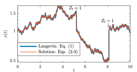
Figure 1: srGBM dynamics. Position of the particle evolves multiplicatively via Eq. (1) until a random event characterized by $Z_{t}=1$ occurs. At this moment, position is reset to $x_{0}=1$ and the dynamics is renewed. The blue line describes a numerical simulation of the Langevin equation (1), whereas the orange line is the solution (2) and (3). In this example, we set $\mu=0.05$, $\sigma^{2}=0.02$ and $r=0.16$.

II.2 Method of simulation

The basic ingredient used to numerically simulate srGBM is to generate a trajectory using Eq. (1). This is done à la Langevin. Concretely, to obtain the distribution of the position of the particle at time $t$, we discretize the time $t=n\Delta t$, where $n$ is an integer. We initialize the position of the particle at $x(0)=1$, and then, at each step ($\tau=1,\dots,n$), the particle can either reset or it can evolve according to the laws of GBM. Thus,

1. with probability $1-r\Delta t$ ($r$ is the rate of resetting), the particle undergoes GBM so that

   $$x(\tau\Delta t)=x((\tau-1)\Delta t)+x((\tau-1)\Delta t)\left[\mu+\sigma\sqrt{\Delta t}\eta(\tau\Delta t)\right],$$ (5)

   where $\eta(\Delta t)$ is a Gaussian random variable with mean $0$ and variance $1$, and $\Delta t$ is the microscopic time step;

2. with complementary probability $r\Delta t$, resetting occurs such that

   $$x(\tau\Delta t) =x(0)=1.$$ (6)

In Fig. 1 we have compared Eq. (3) with the Langevin simulation to find an excellent match.

III Non-equilibrium properties of GBM under stochastic resetting

In this section, we discuss non-equilibrium properties of GBM subjected to stochastic resetting. We first present exact results for the moments at all times. Next, we discuss the non-equilibrium steady state of GBM under stochastic resetting.

III.1 Moments

Moments of srGBM can be computed easily by applying the law of total expectation. In practice, the $m$-th moment is obtained by raising Eq. (3) to the $m$-th power and then averaging with respect to the noise and $f(t_{l}|t)$ respectively

$$\left\langle x^{m}(t)\right\rangle=x_{0}^{m}e^{\left(m\mu+m(m-1)\frac{\sigma^{2}}{2}\right)t}\left\langle e^{-\left(m\mu+m(m-1)\frac{\sigma^{2}}{2}\right)t_{l}(t)}\right\rangle_{t_{l}}$$

$$=\frac{x_{0}^{m}}{m\mu+m(m-1)\frac{\sigma^{2}}{2}-r}\left[\mu\,e^{\left(m\mu+m(m-1)\frac{\sigma^{2}}{2}-r\right)t}-r\right].$$ (7)

In general, three regimes for the evolution of the $m$-th moment can be identified based on the relation between the drift, noise amplitude and the resetting rate. First, when $r>r_{m}\equiv m\mu+m(m-1)\frac{\sigma^{2}}{2}$, the $m$-th moment converges to a limiting value $r/\left(r-r_{m}\right)$. At $r=r_{m}$, a sharp transition occurs, and the moment diverges linearly in time, i.e., $\langle x^{m}(t)\rangle\sim 1+rt$. For $r<r_{m}$, this divergence becomes exponential. Table 1 summarizes the relationship between the parameters and the resulting behavior for the first two moments, i.e., the ensemble average and the second moment. The different limiting points of divergence for the moments can be seen as a hallmark multiplicative property of srGBM. For completeness we present a complementary renewal based derivation for the moments in Appendix A.

Table 1: Moments behavior in srGBM.

Moment	Limiting behavior
	Exponential	Linear	Convergence
	divergence	divergence
$\langle x(t)\rangle$	$r<\mu$	$r=\mu$	$r>\mu$
Eq. (44)	($\sim e^{(\mu-r)t}$)	($\sim rt$)	($\sim r/(r-\mu)$)
$\langle x^{2}(t)\rangle$	$r<2\mu+\sigma^{2}$	$r=2\mu+\sigma^{2}$	$r>2\mu+\sigma^{2}$
Eq. (47)	($\sim e^{(2\mu+\sigma^{2}-r)t}$)	($\sim rt$)	($\sim r/(r-2\mu-\sigma^{2})$)

III.2 Probability Density Function

The probability density function (PDF) of a reset-process satisfies the following renewal equation [11]

$$P_{r}(x,t|x_{0}) =e^{-rt}P_{0}(x,t|x_{0})+r\int_{0}^{t}e^{-ru}P_{0}(x,u|x_{0})\,du,$$ (8)

where $P_{0}(x,t|x_{0})$ is the PDF of the reset-free ($r=0$) process and in case of GBM reads [5, 58]

$$P_{0}(x,t|x_{0}) =\frac{1}{x\sqrt{2\pi\sigma^{2}t}}\exp\left(\frac{-\left[\log(\frac{x}{x_{0}})-(\mu-\frac{\sigma^{2}}{2})t\right]^{2}}{2\sigma^{2}t}\right).$$ (9)

The steady state is then found by taking Laplace transform of Eq. (8), i.e., $P_{r}^{ss}(x|x_{0})=\lim_{t\to\infty}P_{r}(x,t|x_{0})=r\hat{P}_{0}(x,r|x_{0})$, where $\hat{P}_{0}(x,s|x_{0})\equiv\int_{0}^{\infty}e^{-st}P_{0}(x,t|x_{0})\,dt$. Following this (see Appendix B), we find that the stationary distribution has a power law whose right tail is given by

$$P_{r}^{ss}(x|x_{0})\sim C(x_{0})x^{-\alpha-1}\quad\textrm{if}\quad x>x_{0},$$ (10)

for some normalizing constant $C(x_{0})$ that is dependent on the initial condition and a shape parameter

$$\alpha =\frac{-(\mu-\sigma^{2}/2)+\sqrt{(\mu-\sigma^{2}/2)^{2}+2r\sigma^{2}}}{\sigma^{2}}.$$ (11)

The attained stationarity is not enough to render the model ergodic. In standard GBM, non-ergodicity arises due to the noise induced fluctuations which exhibit a net-negative effect on the time-averaged particle position, but do not affect the ensemble average. Therefore, in order to observe stationary-like behavior on the long run one must track the evolution of an infinite number of trajectories [59]. Introducing stochastic resetting does not alter this phenomenon. This is because the long time average of a finite sample of trajectories (defined below) will be dominated by extremely rare non-reset trajectories. However, as will be shown below, resetting represents an additional source of randomness that not only increases the net-negative effect on the time-averaged position but also under certain circumstances may induce a similar effect on the ensemble average. As a result, we observe a variety of long-time regimes for the sample average due to resetting. We discuss these issues next.

IV Ergodic properties

In srGBM, the non-ergodicity of the sample average is manifested in the same way as in GBM, that is, by the difference between the time-average and ensemble growth rate [6]. This is captured by the following estimator of the growth rate of a sample of GBM trajectories

$$g_{est}(t,N) \equiv\frac{1}{t}\log\left(\langle x(t)\rangle_{N}\right),$$ (12)

where

$$\langle x(t)\rangle_{N}=\frac{1}{N}\sum_{i=1}^{N}x_{i}(t)$$ (13)

is known as the finite sample average with the property $\lim_{N\to\infty}\langle x(t)\rangle_{N}=\langle x(t)\rangle$. Similar estimator was used to study ergodic properties in continuous time random walk [59] and anomalous diffusion in disordered materials [60].

The ensemble growth rate $\langle g\rangle$ is found by fixing the period $t$ and taking the limit as the sample grows infinitely, i.e.,

$$\langle g\rangle =\lim_{N\to\infty}g_{est}(t,N).$$ (14)

On the other hand, the time-average growth rate $\bar{g}$ is found by fixing the sample size $N$ and letting time remove the stochasticity,

$$\bar{g} =\lim_{t\to\infty}g_{est}(t,N).$$ (15)

The non-ergodicity of the process is manifested in the non-commutativity of the two limits. Concretely, it can be shown that the ensemble average growth rate is $\langle g\rangle=g(t)$, which can be obtained by substituting Eq. (7) with $m=1$ in Eq. (12). On the other hand, we find that the time average growth rate is $\bar{g}=0$. Let us first present a proof for the simplest case $N=1$, and afterwards generalize the results for arbitrary sample sizes. We start by substituting the solution $x(t)$ from Eq. (3) into Eq. (12) to obtain (setting $x_{0}=1$)

$$g_{est}(t,N=1) =\left(\mu-\frac{\sigma^{2}}{2}\right)\left(1-\frac{t_{l}}{t}\right)+\frac{\sigma}{t}\left(W(t)-W(t_{l})\right),$$ (16)

from where it follows that (Appendix C)

$$\left\langle g_{est}(t,N=1)\right\rangle =\left(\mu-\frac{\sigma^{2}}{2}\right)\left(1-\frac{\langle t_{l}\rangle}{t}\right),$$ (17)

and

$$\text{Var}\left[g_{est}(t,N=1)\right] =\left(\mu-\frac{\sigma^{2}}{2}\right)^{2}\frac{\text{Var}\left[t_{l}\right]}{t^{2}}+\frac{\sigma^{2}}{t}\left(1-\frac{\langle t_{l}\rangle}{t}\right),$$ (18)

where ‘Var’ stands for variance. These results hold for any resetting time density. In particular, for Poissonian resetting, $\left\langle g_{est}(t,N=1)\right\rangle=\text{Var}\left[g_{est}(t,N=1)\right]=0$ in the limit $t\to\infty$. This essentially implies that the distribution of $g_{est}(t,N=1)$ must converge to a Dirac delta function asymptotically. In other words, as $t\to\infty$, the observed growth rate $\bar{g}$ will differ from $0$ with probability zero.

The proof for arbitrary $N$ is based on extreme value theory [6, 61]. In particular, we will show that $\bar{g}$ is bounded from above and below, and that these bounds coincide. The upper bound can be shown by observing that for a fixed $t$ and sample size $N$

$$g_{est}(t,N)\leq\max_{i}\frac{1}{t}\log x_{i}(t)=\max_{i}g_{est}^{\left[i\right]}(t,N=1),$$ (19)

since the system size is finite. Taking the limit with respect to time, it follows that

$$\bar{g}\leq\max_{i}\lim_{t\to\infty}g_{est}^{\left[i\right]}(t,N=1)=0.$$ (20)

In a similar manner, for the lower bound we have

$$\bar{g}\geq\min_{i}\lim_{t\to\infty}g_{est}^{\left[i\right]}(t,N=1)=0.$$ (21)

Hence, the bounds for $\bar{g}$ saturate to a threshold which is zero implying $\bar{g}=0$ for any fixed sample size.

To numerically illustrate this non-ergodicity, we plot the long run sample average $\langle x(t)\rangle_{N}$ as a function of resetting rate $r$ for various sample sizes in Fig. 2. We simulate the sample average by generating $N$ independent and identical copies of the Langevin simulation, i.e.,

$$\langle x(\tau\Delta t)\rangle_{N} =\frac{\sum_{i}^{N}x_{i}(\tau\Delta t)}{N}.$$ (22)

As described in the main text, $\langle x(\tau\Delta t)\rangle_{N}$ will resemble the ensemble average as long as $\tau\Delta t<t_{c}$, and afterwards it will collapse to its time-average behavior.

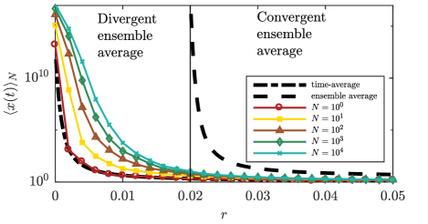
Figure 2: Ergodicity breaking in srGBM. Long time sample average ($t=10^{5}$) as a function of $r$ for various sample sizes. For each sample size, $10^{4}$ random realizations were generated and the median results are shown. We set $\mu=0.02$, $\sigma^{2}=0.01$. The black vertical line indicates the threshold $r=\mu$ where the ensemble average becomes convergent.

For $r\leq\mu$, the ensemble average diverges (dashed black line). However, the time-average is convergent resulting in the sample average to converge. Even in the regime when $r>\mu$ the sample average is closer to the time-average and there are apparent differences with the ensemble average. This is best seen in the single system (marked with a circle), which is dominated by the time-average behavior (dash-dotted black line). As the sample size increases, the sample average draws closer to the magnitude of the ensemble average but it always remains convergent.

To explain the differences in observations belonging to different sample sizes one can use an analogy with Random Energy Model (REM) studied by Derrida [57, 62]. In REM, there exists a critical inverse temperature $t_{c}$ below which the quenched and annealed averages are identical whereas above $t_{c}$, only the quenched average is observed and the system is frozen in a small number of configurations of energy [63]. In srGBM, $t_{c}$ corresponds to a critical self-averaging time until which the sample average resembles the corresponding ensemble value, i.e., the time until Eq. (14) is valid. However, note that in the absence of resetting, the critical self-averaging time is strictly determined by and is proportional with the sample size. Hence, as the sample size increases the sample average will spend longer time resembling the ensemble average. These dynamics are accumulated and effectively reflected in the observed time-average at the end. In stark contrast, we show that in srGBM, $t_{c}$ depends on both the sample size and the resetting strength and thus resulting in different long-time regimes. This is discussed next.

V Self-averaging properties

In srGBM, the critical self-averaging time can be estimated by the relative variance of the sample average, namely,

$$\mathrm{R}_{N}(t) \equiv\frac{\text{Var}(\langle x(t)\rangle_{N})}{\langle\langle x(t)\rangle_{N}\rangle^{2}},$$ (23)

where $\langle\cdot\rangle$ and $\text{Var}(\cdot)$ notations, without $N$ as a subscript, refer to the averages over all possible sample average realizations. Using Eq. (13) and the property for variance of sums of IID random variables, Eq. (23) can be rewritten as

$$\mathrm{R}_{N}(t) =\frac{1}{N}\frac{\langle x^{2}(t)\rangle-\langle x(t)\rangle^{2}}{\langle x(t)\rangle^{2}}.$$ (24)

If $\mathrm{R}_{N}(t)\ll 1$, the system is self-averaging, i.e., the sample average will be close to the ensemble average. Thus, the system will be self-averaging until the critical point $t_{c}$ which occurs at $\mathrm{R}_{N}(t_{c})=1$. We can use this information and rephrase Eq. (24) as

$$N+1 =\frac{\langle x^{2}(t_{c})\rangle}{\langle x(t_{c})\rangle^{2}},$$ (25)

which is the governing relation to determine $t_{c}$. This is done by plotting Eq. (25) as a function of $r$ in Fig. 3(a). Starting at $r=0$, the self-averaging time $t_{c}$ first decreases and then increases as a a function of resetting rate $r$. Depending on the trade-off between resetting rate ($r$), drift ($\mu$) and noise strength ($\sigma$), the system exhibits three different regimes which we explore in the following.

V.1 Frozen state

In the regime $r<\mu$, if we were to start with $N$-microstates with equally distributed energies, during the self-averaging period, inequality will increase and the system will eventually end up in a frozen configuration, as in REM. This is because both the ensemble average, given by Eq. (44) [putting $m=1$ in Eq. (7)], and the second moment, given by Eq. (47) [putting $m=2$ in Eq. (7)], are divergent. Thus, we can respectively approximate them as

$$\langle x(t)\rangle \approx\frac{\mu}{\mu-r}\exp\left[\left(\mu-r\right)t\right]x_{0},$$ (26)

and

$$\langle x^{2}(t)\rangle\approx\frac{2\mu+\sigma^{2}}{2\mu+\sigma^{2}-r}\exp\left[(2\mu+\sigma^{2}-r)t\right]x_{0}^{2}.$$ (27)

Putting these two equations in Eq. (25) we can get an approximate equation for the critical self-averaging time in this regime as

$$t_{c}\approx\frac{1}{r+\sigma^{2}}\log\left[(N+1)\frac{\mu^{2}(2\mu+\sigma^{2}-r)}{(\mu-r)^{2}(2\mu+\sigma^{2})}\right].$$ (28)

For a large enough sample this reduces to

$$t_{c}\approx\frac{1}{r+\sigma^{2}}\log\left[(N+1)\right],$$ (29)

which is precisely the behavior observed in Fig. 3(a).

We quantify the degree of freezing with the probability $P_{1\%}(t)$ that the system occupies a microstate that is among the largest 1% of the sampled particle energies in time $t$ (Fig. 3(b)). Numerically, this is easily done by relabeling the $N$ trajectories i.e., without loss of generality we assume that $x_{1}(\tau\Delta t)\geq x_{2}(\tau\Delta t)\geq\dots\geq x_{N}(\tau\Delta t)$. Then, $P_{1\%}(\tau\Delta t)$ in the period $\tau\Delta t$ is estimated as

$$P_{1\%}(\tau\Delta t) =\frac{\sum_{j}^{N/100}x_{j}(\tau\Delta t)}{\sum_{i}^{N}x_{i}(\tau\Delta t)}.$$ (30)

In the economics literature, $P_{1\%}$ is interpreted as a measure of income inequality and its observed dynamics are expressed through changes in the model parameters, reflecting shocks (changes in model parameters due to external forces) in the system conditions [64, 55]. Thus, a value of $P_{1\%}$ closer to unity indicates a frozen configuration. An example for how $P_{1\%}$ behaves as a function of time is given in Fig. 3(c) with a dashed line.

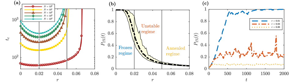
Figure 3: Self-averaging in srGBM. (a) Critical self-averaging time $t_{c}$ as a function of $r$ for various sample sizes $N$. $t_{c}$ is seen to be minimized at $r^{*}=\mu$ for large sample size. The vertical lines indicate the thresholds $r=\mu$ and $r=2\mu+\sigma^{2}$ at which the ensemble average and second moment respectively become convergent. (b) Long time ($t=10^{5}$) probability of observing a microstate that is among the largest 1% averaged across $10^{4}$ simulations. The median results are shown, and the filled region is the 5th and 95th percentile. Three regimes correspond to (i) $r<\mu$ (frozen), (ii) $2\mu+\sigma^{2}>r>\mu$ (unstable annealed) and (iii) $r>2\mu+\sigma^{2}$ (stable annealed). (c) Statistics of example simulations for the probability of observing a a microstate that is among the largest 1%. Different colors indicate the regimes mentioned in (b). Parameters: $\mu=0.02$, $\sigma^{2}=0.01$ and $N=10^{4}$.

V.2 Unstable state

In the regime when $\mu<r<2\mu+\sigma^{2}$ the ensemble average, given by Eq. (44), is converges to a stationary value, whereas the second moment, given by Eq. (47), remains divergent. Specifically, then the ensemble average is approximated as

$$\langle x(t)\rangle \approx\frac{r}{r-\mu}x_{0},$$ (31)

while the evolution of the second moment remains the same as in Eq. (27). Putting these two equations in Eq. (25), we find the critical self-averaging time to be

$$t_{c}\approx\frac{1}{2\mu+\sigma^{2}-r}\log\left[(N+1)\frac{r^{2}(2\mu+\sigma^{2}-r)}{(r-\mu)^{2}(2\mu+\sigma^{2})}\right].$$ (32)

Again, for a large enough sample the above equation reads

$$t_{c}\approx\frac{1}{2\mu+\sigma^{2}-r}\log\left[(N+1)\right].$$ (33)

which is clearly an increasing function of $r$, as can be seen in Fig. 3(a). In words, beyond $r>\mu$, increments in $r$ reflect in an increased self-averaging time. Since $t_{c}$ is a decreasing function of resetting rate $r$ when $r<\mu$ and an increasing function when $\mu<r<2\mu+\sigma^{2}$, it must be the case that the function attains a a local minimum on the interval $\left[0,2\mu+\sigma^{2}\right]$ at the point $r^{*}=\mu$. Note that the transition point coincides with the threshold required for the ensemble average to become convergent. This is indeed observed in Fig. 3(a). We remark that for a small sample size, the optimal resetting rate $r^{*}$ that minimizes $t_{c}$, is weakly dependent on the sample size $N$. Therefore, optimization of $t_{c}$ with respect to resetting rate $r$ is one of the central features of this work.

Moreover, in this state, the resetting rate is large enough to squeeze the effect of the drift and constrain the ensemble average, but the second moment remains divergent. Due to this, after the self-averaging period even if the particle’s position is reset, it will quickly return to its pre-resetting position. Thus the system will not always be trapped in a small number of configurations (Fig. 3(b)). Instead, the share $P_{1\%}$ will randomly phase between large and small values over time. This, in turn implies that the state of the configurations will be unstable over time as evidenced in Fig. 3(c), with the dash dotted line. This is a significant impact of resetting on the long time behavior of GBM.

V.3 Stable state

As $r$ is further increased and above $2\mu+\sigma^{2}$, the second moment also becomes convergent and a third regime appears. In this case, in the long time limit the second moment is convergent and reads

$$\langle x^{2}(t)\rangle\approx\frac{r}{r-2\mu-\sigma^{2}}x_{0},$$ (34)

By combining the above equation with Eq. (31), we get that the long time relative variance in this regime is approximately constant

$$R_{N}(t)\approx\frac{1}{N}\left[\frac{(r-\mu)^{2}}{r(r-2\mu-\sigma^{2})}-1\right].$$ (35)

It can be observed that in this case the sample average resembles the ensemble value (Fig. 3(a)) and exhibits diverse configurations (Fig. 3(b)). Consequently, the probability $P_{1\%}$ of observing extreme configurations stabilizes over time (Fig. 3(c) dotted line). This is the onset of a stable annealed regime. In this state, for a large enough sample size $N$, the system may forever mimic ergodic behavior. More precisely, self-averaging will always occur in the system if $R_{N}(t)$ in Eq. (35) is less than one. This leads to the condition

$$N>\frac{\mu^{2}+r\sigma^{2}}{(r-2\mu-\sigma^{2})r},$$ (36)

This is remarkably different from the previous two regimes, where for any fixed sample size, we would eventually observe discrepancies between the ensemble and sample averages, and is another important feature induced by resetting on GBM.

VI Conclusion

In this work, we performed a detailed analysis on the spatial and ergodic properties of srGBM. While discrete time stochastic and deterministic multiplicative processes with resetting have been studied in [27, 28], a detailed and systematic investigation for the spatial and ergodic properties for the continuous time multiplicative process such as GBM was still missing. The emergence of three regimes namely frozen/quenched, an unstable and a stable annealed state is especially noteworthy. The ensemble properties of the second and third regime have been explored to a great extent in the income inequality literature [55]. Indeed, most identified power laws in nature have exponents such that the average is well-defined but the variance is not, implying that the second regime is an expected outcome [65]. Nonetheless, recent studies in economics also identify non-ergodic and divergent behavior in samples of srGBM trajectories thus suggesting the existence of the first regime [66, 50]. A typical example of srGBM would be investment portfolios with reconstitution (addition or removal of constituents) [67] where one might observe a such multi-stable landscape. Naturally, the results presented here for srGBM lend themselves as a baseline to depict the long run behavior of the above-mentioned scenarios. This empirical investigation represents an intriguing research question which we leave for future work.

From a technical perspective, it is important to stress that the solution (3), time-average growth rate (16), and the critical self-averaging time (25) are universal and do not depend on the resetting time density. It remains to be seen how the statistical properties of GBM alter intricately under arbitrary resetting time density. Moreover, the dependence of $t_{c}$ on generic resetting time distribution suggests that we may observe diverse properties for the optimality based on the resetting strategy that we employ (similar to various optimization of the mean first passage time under resetting [30]). Finally, GBM, besides being a canonical model for self-reproduction, is also used to describe diffusion processes where the particle spreads very fast, such as heterogeneous and turbulent diffusion [68, 69]. Exploring the applications of resetting strategies on GBM thus also represents a potential research avenue that is of broad interest.

Appendix A Calculation of moments for srGBM

In the main text we showed how to derive the moments of srGBM using the law of total expectation. In this section, we present alternative derivations for the moments using Fokker-Planck and a renewal approach respectively.

A.1 Fokker-Planck approach

The Fokker-Planck equation for the GBM with exponential resetting to the initial position $P_{r}(x,t=0|x_{0})=\delta(x-x_{0})$ reads

$$\frac{\partial}{\partial t}P_{r}(x,t|x_{0})=-\mu\frac{\partial}{\partial x}xP_{r}(x,t|x_{0})+\frac{\sigma^{2}}{2}\frac{\partial^{2}}{\partial x^{2}}x^{2}P_{r}(x,t|x_{0})-rP_{r}(x,t|x_{0})+rP_{r}(x,t=0|x_{0}),$$ (37)

where $r$ is the rate of resetting to the initial position $x_{0}$. The last two terms in the RHS of Eq. (37) represent respectively the loss of the probability from position $x\neq x_{0}$ due to the resetting and consecutively a gain in the probability at the initial position $x_{0}$ from all the other positions in space. Taking Laplace transform on both sides of Eq. (37) gives

$$s\hat{P_{r}}(x,s|x_{0})-P_{r}(x,t=0|x_{0})=-\mu\frac{\partial}{\partial x}x\hat{P_{r}}(x,s|x_{0})+\frac{\sigma^{2}}{2}\frac{\partial^{2}}{\partial x^{2}}x^{2}\hat{P_{r}}(x,s|x_{0})-r\hat{P_{r}}(x,s|x_{0})+\frac{r}{s}P_{r}(x,t=0|x_{0}),$$ (38)

where $\hat{g}(s)=\mathcal{L}[g(t)]=\int_{0}^{\infty}g(t)e^{-st}\,dt$ is the Laplace transform of $g(t)$. Rewriting the above equation, one gets

$$s\hat{P_{r}}(x,s|x_{0})-P_{r}(x,t=0|x_{0})=s\times\frac{1}{s+r}\left[-\mu\frac{\partial}{\partial x}x\hat{P_{r}}(x,s|x_{0})+\frac{\sigma^{2}}{2}\frac{\partial^{2}}{\partial x^{2}}x^{2}\hat{P_{r}}(x,s|x_{0})\right],$$ (39)

which, upon an inverse Laplace transform, gives us the following convoluted equation

$$\frac{\partial}{\partial t}P_{r}(x,t|x_{0})=\frac{\partial}{\partial t}\int_{0}^{t}\eta(t-t^{\prime}) \left[-\mu\frac{\partial}{\partial x}xP_{r}(x,t^{\prime}|x_{0})+\frac{\sigma^{2}}{2}\frac{\partial^{2}}{\partial x^{2}}x^{2}P_{r}(x,t^{\prime}|x_{0})\right]dt^{\prime},$$ (40)

where $\eta(t)=e^{-rt}$. Note that a similar equation was also used in Ref. [58] to explore the properties of a generalized GBM process subject to subdiffusion (without resetting). In what follows, we would like to write a dynamical equation for the moments $\langle x^{m}(t)\rangle\equiv\int_{0}^{\infty}~{}x^{m}(t)P_{r}(x,t|x_{0})~{}dx$ using Eq. (40). To see this, we multiply both sides of Eq. (40) by $x^{m}$ and integrate over $x$ to find

$$\frac{\partial}{\partial t}\langle x^{m}(t)\rangle=\left[\frac{\sigma^{2}}{2}m(m-1)+\mu\,m\right]\mu\,\frac{d}{dt}\int_{0}^{t}\eta(t-t^{\prime})\langle x^{m}(t^{\prime})\rangle\,dt^{\prime}.$$ (41)

In Laplace space, the solution to this equation reads

$$\langle\hat{x}^{m}(s)\rangle=\frac{s^{-1}}{1-\hat{\eta}(s)\left[\frac{\sigma^{2}}{2}m(m-1)+\mu\,m\right]}x_{0}^{n},$$ (42)

where $\hat{\eta}(s)=\mathcal{L}\left[e^{-rt}\right]=\frac{1}{s+r}$, and $x_{0}=x(0)$ is the fixed initial condition. For $m=1$, the solution of the equation for the ensemble average (first moment or the mean value) in Laplace space is given by

$$\left\langle\hat{x}(s)\right\rangle=\frac{s^{-1}}{1-\mu\hat{\eta}(s)}x_{0}=\frac{s^{-1}}{1-\mu/(s+r)}x_{0},$$ (43)

which can be inverted to obtain the following expression for the mean

$$\left\langle x(t)\right\rangle=\frac{x_{0}}{\mu-r}\left[\mu\,e^{\left(\mu-r\right)t}-r\right],$$ (44)

Similarly, for $m=2$, using Eq. (41), we obtain the following equation for the second moment

$$\frac{\partial}{\partial t}\langle x^{2}(t)\rangle=(\sigma^{2}+2\mu)\frac{d}{dt}\int_{0}^{t}\eta(t-t^{\prime})\langle x^{2}(t^{\prime})\rangle\,dt^{\prime},$$ (45)

with a solution in Laplace space

$$\langle\hat{x}^{2}(s)\rangle=\frac{s^{-1}}{1-(\sigma^{2}+2\mu)\hat{\eta}(s)}x_{0}^{2}=\frac{s^{-1}}{1-(\sigma^{2}+2\mu)/(s+r)}x_{0}^{2},$$ (46)

which can be inverted to obtain the following expression for the second moment

$$\left\langle x^{2}(t)\right\rangle=\frac{x_{0}^{2}}{2\mu+\sigma^{2}-r}\left[(2\mu+\sigma^{2})\,e^{(2\mu+\sigma^{2}-r)t}-r\right].$$ (47)

Finally, inverting Eq. (42), we arrive at Eq. (7) as was mentioned in the main text.

A.2 Renewal approach

It is now well understood that resetting is a renewal process in the sense the process erases its memory after each resetting. This leads to an advantage since the solution of the reset-process $P_{r}(x,t|x_{0},0)$ can be written in terms of the underlying reset-free process $P_{0}(x,t|x_{0},0)$. Following Ref. [11], we can write

$$P_{r}(x,t|x_{0},0) =e^{-rt}P_{0}(x,t|x_{0},0)+\int_{0}^{t}~{}re^{-ru}~{}P_{0}(x,u|x_{0},0)\,du,$$ (48)

which is essentially Eq. (8). This equation can be interpreted in terms of a renewal process, i.e., each resetting event to the initial position $x_{0}$ renews the process at a rate $r$. Between two consecutive renewal events, the particle undergoes its original dynamics. In fact Eq. (48) can also be obtained from Eq. (40) using a subordination approach used in [58]. To show this, note that the solution of Eq. (40) can be represented by the subordination integral

$$P_{r}(x,t|x_{0})=\int_{0}^{\infty}P_{0}(x,u|x_{0})\,h(u,t)\,du,$$ (49)

where $h(u,t)$ is a subordination function. For the present case of exponential waiting time for resetting, the subordination function for srGBM reads, see Ref. [58],

$$\hat{h}(u,s)=\frac{1}{s\hat{\eta}(s)}e^{-\frac{u}{\hat{\eta}(s)}}=\frac{s+r}{s}e^{-u(s+r)}\quad\rightarrow\quad h(u,t)=e^{-rt}\delta(t-u)+r\,e^{-ru}\theta(t-u).$$ (50)

Thus

$$P_{r}(x,t|x_{0})= \int_{0}^{\infty}P_{0}(x,t|x_{0},0)\left[e^{-rt}\delta(t-u)+r\,e^{-ru}\theta(t-u)\right]du$$ (51)

from where we recover the renewal form given in Eq. (48). Taking Laplace transform on the both sides of the above equation gives

$$\hat{P_{r}}(x,s|x_{0})=\hat{P}_{0}(x,s+r|x_{0})+\frac{r}{s}\hat{P}_{0}(x,s+r|x_{0})=\frac{s+r}{s}\hat{P}_{0}(x,s+r|x_{0}),$$ (52)

where $\hat{P}_{0}(x,s)$ is the Laplace transform of the underlying propagator. By multiplying Eq. (52) with $x^{m}(s)$ and integrating out $x$, the $m$-th moment of srGBM in Laplace space can be written as

$$\left\langle\hat{x}^{m}(s)\right\rangle =\frac{s+r}{s}\left\langle\hat{x}^{m}(s+r)\right\rangle_{r=0},$$ (53)

where $\left\langle\hat{x}^{m}(s)\right\rangle_{r=0}$ is the $m$-th moment without resetting in the Laplace space. Note that the equations derived so far do not depend on the specific choice of underlying dynamics. Moving forward, we will turn our focus to the GBM process. In particular, the GBM-propagator reads

$$P_{0}(x,t|x_{0},0) =\frac{1}{x\sqrt{2\pi\sigma^{2}t}}\exp\left(-\frac{\left[\log(\frac{x}{x_{0}})-(\mu-\frac{\sigma^{2}}{2})t\right]^{2}}{2\sigma^{2}t}\right),$$ (54)

which is a log-normal distribution. The moments, obtained from Eq. (54), read

$$\left\langle x^{m}(t)\right\rangle_{r=0}=x_{0}^{m}\,e^{\left(\sigma^{2}m(m-1)/2+\mu m\right)t}.$$ (55)

Computing the Laplace transforms $\left\langle\hat{x}^{m}(s)\right\rangle_{r=0}$ from above and substituting into Eq. (53) gives us the moments of srGBM in Laplace space. Inverting them, we recover the results as given by Eq. (7).

Appendix B Full expression for the stationary distribution

In this section, we provide the full expressions for the steady state. To this end, we recall Eq. (48) and take the limit $t\to\infty$. The first term on the RHS of Eq. (48) drops out and we are left with

$$P_{r}^{ss}(x|x_{0})=\lim_{t\rightarrow\infty}P_{r}(x,t|x_{0})=\int_{0}^{\infty}~{}re^{-ru}~{}P_{0}(x,u|x_{0},0)\,du=r\hat{P}_{0}(x,r|x_{0}).$$ (56)

Thus to compute the steady state, we need the Laplace transform of the underlying propagator. In particular, for GBM, they can be computed from Eq. (54). Eventually, we have

$$\hat{P}_{0}(x,s|x_{0})=\frac{1}{\sqrt{(\mu-\sigma^{2}/2)^{2}+2\sigma^{2}s}}\left\{\begin{array}[]{l l l}\vskip 3.0pt plus 1.0pt minus 1.0pt&\left(\frac{x}{x_{0}}\right)^{-\frac{\sqrt{(\mu-\sigma^{2}/2)^{2}+2\sigma^{2}s}-(\mu-\sigma^{2}/2)}{\sigma^{2}}-1},&x>x_{0},\\ &\left(\frac{x}{x_{0}}\right)^{\frac{\sqrt{(\mu-\sigma^{2}/2)^{2}+2\sigma^{2}s}+(\mu-\sigma^{2}/2)}{\sigma^{2}}-1},&x\leq x_{0}.\end{array}\right.$$ (59)

Thus, using Eq. (56), we arrive at the following expressions for the non-equilibrium steady state for srGBM

$$P_{r}^{ss}(x|x_{0})=\frac{r\sigma^{2}}{\alpha\sigma^{2}+\left(\mu-\frac{\sigma^{2}}{2}\right)}\left\{\begin{array}[]{l l l}\vskip 3.0pt plus 1.0pt minus 1.0pt&\left(\frac{x}{x_{0}}\right)^{-\alpha-1},&x>x_{0},\\ &\left(\frac{x}{x_{0}}\right)^{\alpha+2\left(\mu-\frac{\sigma^{2}}{2}\right)-1},&x\leq x_{0},\end{array}\right.$$ (62)

where

$$\alpha =\frac{-(\mu-\sigma^{2}/2)+\sqrt{(\mu-\sigma^{2}/2)^{2}+2r\sigma^{2}}}{\sigma^{2}},$$ (63)

is the shape parameter. The right tail ($x>x_{0}$) of this result has been highlighted in Eq. (10) in the main text.

Appendix C Calculation of moments for the srGBM growth rate

Here we derive the moments of the srGBM growth rate given in Eqs. (17) and (18). We start by noting that the estimator of the growth rate when $N=1$ can be found by inputting Eq. (3) in Eq. (12), i.e.,

$$g_{est}(t,N=1) =\left(\mu-\frac{\sigma^{2}}{2}\right)\left(1-\frac{t_{l}}{t}\right)+\frac{\sigma}{t}\left(W(t)-W(t_{l})\right),$$ (64)

where for simplicity we have set $x(0)=1$. In order to derive the moments of srGBM, we are going to utilize three basic properties of the Wiener process. That is, the process is characterized with a first moment, $\langle W(t)\rangle=0$, second moment $\langle W^{2}(t)\rangle=t$, and a covariance $\langle W(t)W(s)\rangle=\min\{t,s\}$.

Using this information, we can average Eq. (64) first with respect to the Wiener noise, and then with respect to $t_{l}$ to get the first moment

$$\left\langle g_{est}(t,N=1)\right\rangle =\left(\mu-\frac{\sigma^{2}}{2}\right)\left(1-\frac{\langle t_{l}\rangle}{t}\right).$$ (65)

To derive the variance, we first square Eq. (64), and get

$$g_{est}^{2}(t,N=1) =\left(\mu-\frac{\sigma^{2}}{2}\right)^{2}\left(1-\frac{t_{l}}{t}\right)^{2}+2\left(\mu-\frac{\sigma^{2}}{2}\right)\left(1-\frac{t_{l}}{t}\right)\frac{\sigma}{t}\left(W(t)-W(t_{l})\right)+\frac{\sigma^{2}}{t^{2}}\left(W(t)-W(t_{l})\right)^{2}.$$ (66)

Again, we take the average of Eq. (66) first with respect to the Wiener noise, and then with respect to $t_{l}$. The computation goes as follows

$$\left\langle g_{est}^{2}(t,N=1)\right\rangle =\left(\mu-\frac{\sigma^{2}}{2}\right)^{2}\left\langle\left(1-\frac{t_{l}}{t}\right)^{2}\right\rangle+2\left(\mu-\frac{\sigma^{2}}{2}\right)\left(1-\frac{\langle t_{l}\rangle}{t}\right)\frac{\sigma}{t}\left(\left\langle W(t)\right\rangle-\left\langle W(t_{l})\right\rangle\right)+\frac{\sigma^{2}}{t^{2}}\left\langle\left(W(t)-W(t_{l})\right)^{2}\right\rangle$$ (67)

$$=\left(\mu-\frac{\sigma^{2}}{2}\right)^{2}\left\langle\left(1-\frac{t_{l}}{t}\right)^{2}\right\rangle+\frac{\sigma^{2}}{t^{2}}\left(\left\langle W^{2}(t)\right\rangle-\left\langle W(t)W(t_{l})\right\rangle+\left\langle W^{2}(t_{l}\right\rangle\right)$$ (68)

$$=\left(\mu-\frac{\sigma^{2}}{2}\right)^{2}\left\langle\left(1-\frac{t_{l}}{t}\right)^{2}\right\rangle+\frac{\sigma^{2}}{t}\left(1-\frac{\langle t_{l}\rangle}{t}\right).$$ (69)

where we have used properties of the Wiener process. Finally, variance of $g_{est}(t,N=1)$, as given in Eq. (18) in the main text, is recovered from the following

$$\text{Var}\left[g_{est}(t,N=1)\right] =\left\langle g_{est}^{2}(t,N=1)\right\rangle-\left\langle g_{est}(t,N=1)\right\rangle^{2}$$ (70)

$$=\left(\mu-\frac{\sigma^{2}}{2}\right)^{2}\frac{\text{Var}\left[t_{l}\right]}{t^{2}}+\frac{\sigma^{2}}{t}\left(1-\frac{\langle t_{l}\rangle}{t}\right),$$ (71)

where $\text{Var}\left[t_{l}\right]=\langle t_{l}^{2}\rangle-\langle t_{l}\rangle^{2}$.

References

- Braumann [1983] C. A. Braumann, Population growth in random environments, Bull. Math. Biol. 45, 635 (1983).
- Black and Scholes [1973] F. Black and M. Scholes, The pricing of options and corporate liabilities, J. Polit. Econ. 81, 637 (1973).
- Shah [1997] A. Shah, Black, merton and scholes: Their work and its consequences, Econ. Political Wkly , 3337 (1997).
- Limpert et al. [2001] E. Limpert, W. A. Stahel, and M. Abbt, Log-normal distributions across the sciences: keys and clues: on the charms of statistics, and how mechanical models resembling gambling machines offer a link to a handy way to characterize log-normal distributions, which can provide deeper insight into variability and probability—normal or log-normal: that is the question, BioScience 51, 341 (2001).
- Aitchison and Brown [1957] J. Aitchison and J. A. Brown, The lognormal distribution with special reference to its uses in economics (Cambridge University Press, 1957).
- Peters and Klein [2013] O. Peters and W. Klein, Ergodicity breaking in geometric brownian motion, Phys. Rev. Lett. 110, 100603 (2013).
- Cherstvy et al. [2017] A. G. Cherstvy, D. Vinod, E. Aghion, A. V. Chechkin, and R. Metzler, Time averaging, ageing and delay analysis of financial time series, New J. Phys. 19, 063045 (2017).
- Zipf [2016] G. K. Zipf, Human behavior and the principle of least effort: An introduction to human ecology (Ravenio Books, 2016).
- Evans and Majumdar [2011a] M. R. Evans and S. N. Majumdar, Diffusion with stochastic resetting, Phys. Rev. Lett. 106, 160601 (2011a).
- Evans and Majumdar [2011b] M. R. Evans and S. N. Majumdar, Diffusion with optimal resetting, J. Phys. A: Math. Theor. 44, 435001 (2011b).
- Evans et al. [2020] M. R. Evans, S. N. Majumdar, and G. Schehr, Stochastic resetting and applications, J. Phys. A: Math. Theor. 53, 193001 (2020).
- Majumdar et al. [2015] S. N. Majumdar, S. Sabhapandit, and G. Schehr, Dynamical transition in the temporal relaxation of stochastic processes under resetting, Phys. Rev. E 91, 052131 (2015).
- Pal [2015] A. Pal, Diffusion in a potential landscape with stochastic resetting, Phys. Rev. E 91, 012113 (2015).
- Pal et al. [2016] A. Pal, A. Kundu, and M. R. Evans, Diffusion under time-dependent resetting, J. Phys. A: Math. Theor. 49, 225001 (2016).
- Nagar and Gupta [2016] A. Nagar and S. Gupta, Diffusion with stochastic resetting at power-law times, Phys. Rev. E 93, 060102 (2016).
- Basu et al. [2019] U. Basu, A. Kundu, and A. Pal, Symmetric exclusion process under stochastic resetting, Phys. Rev. E 100, 032136 (2019).
- Singh et al. [2020] R. Singh, R. Metzler, and T. Sandev, Resetting dynamics in a confining potential, J. Phys. A: Math. Theor. 53, 505003 (2020).
- Gupta et al. [2020a] D. Gupta, C. A. Plata, and A. Pal, Work fluctuations and jarzynski equality in stochastic resetting, Phys. Rev. Lett. 124, 110608 (2020a).
- Gupta et al. [2020b] D. Gupta, C. A. Plata, A. Kundu, and A. Pal, Stochastic resetting with stochastic returns using external trap, J. Phys. A: Math. Theor. 54, 025003 (2020b).
- Méndez and Campos [2016] V. Méndez and D. Campos, Characterization of stationary states in random walks with stochastic resetting, Phys. Rev. E 93, 022106 (2016).
- Gupta et al. [2014] S. Gupta, S. N. Majumdar, and G. Schehr, Fluctuating interfaces subject to stochastic resetting, Phys. Rev. Lett. 112, 220601 (2014).
- Evans et al. [2013] M. R. Evans, S. N. Majumdar, and K. Mallick, Optimal diffusive search: nonequilibrium resetting versus equilibrium dynamics, J. Phys. A: Math. Theor. 46, 185001 (2013).
- Magoni et al. [2020] M. Magoni, S. N. Majumdar, and G. Schehr, Ising model with stochastic resetting, Physical Review Research 2, 033182 (2020).
- Durang et al. [2014] X. Durang, M. Henkel, and H. Park, The statistical mechanics of the coagulation–diffusion process with a stochastic reset, J. Phys. A: Math. Theor. 47, 045002 (2014).
- Pal and Rahav [2017] A. Pal and S. Rahav, Integral fluctuation theorems for stochastic resetting systems, Phys. Rev. E 96, 062135 (2017).
- Ray [2020] S. Ray, Space-dependent diffusion with stochastic resetting: A first-passage study, The Journal of Chemical Physics 153, 234904 (2020).
- Manrubia and Zanette [1999] S. C. Manrubia and D. H. Zanette, Stochastic multiplicative processes with reset events, Phys. Rev. E 59, 4945 (1999).
- Zanette and Manrubia [2020] D. Zanette and S. Manrubia, Fat tails and black swans: Exact results for multiplicative processes with resets, Chaos 30, 033104 (2020).
- Kusmierz et al. [2014] L. Kusmierz, S. N. Majumdar, S. Sabhapandit, and G. Schehr, First order transition for the optimal search time of lévy flights with resetting, Phys. Rev. Lett. 113, 220602 (2014).
- Pal and Reuveni [2017] A. Pal and S. Reuveni, First passage under restart, Phys. Rev. Lett. 118, 030603 (2017).
- Meylahn et al. [2015] J. M. Meylahn, S. Sabhapandit, and H. Touchette, Large deviations for markov processes with resetting, Phys. Rev. E 92, 062148 (2015).
- Bodrova et al. [2019] A. S. Bodrova, A. V. Chechkin, and I. M. Sokolov, Scaled brownian motion with renewal resetting, Phys. Rev. E 100, 012120 (2019).
- Pal and Prasad [2019a] A. Pal and V. Prasad, Landau-like expansion for phase transitions in stochastic resetting, Phys. Rev. Research 1, 032001 (2019a).
- Pal and Prasad [2019b] A. Pal and V. Prasad, First passage under stochastic resetting in an interval, Phys. Rev. E 99, 032123 (2019b).
- Chechkin and Sokolov [2018] A. Chechkin and I. Sokolov, Random search with resetting: a unified renewal approach, Phys. Rev. Lett. 121, 050601 (2018).
- Kuśmierz and Gudowska-Nowak [2019] Ł. Kuśmierz and E. Gudowska-Nowak, Subdiffusive continuous-time random walks with stochastic resetting, Phys. Rev. E 99, 052116 (2019).
- Belan [2018] S. Belan, Restart could optimize the probability of success in a bernoulli trial, Phys. Rev. Lett. 120, 080601 (2018).
- Pal et al. [2019] A. Pal, I. Eliazar, and S. Reuveni, First passage under restart with branching, Phys. Rev. Lett. 122, 020602 (2019).
- De Bruyne et al. [2020] B. De Bruyne, J. Randon-Furling, and S. Redner, Optimization in first-passage resetting, Phys. Rev. Lett. 125, 050602 (2020).
- Domazetoski et al. [2020] V. Domazetoski, A. Masó-Puigdellosas, T. Sandev, V. Méndez, A. Iomin, and L. Kocarev, Stochastic resetting on comblike structures, Phys. Rev. Research 2, 033027 (2020).
- Boyer et al. [2017] D. Boyer, M. R. Evans, and S. N. Majumdar, Long time scaling behaviour for diffusion with resetting and memory, J. Stat. Mech. 2017, 023208 (2017).
- Singh and Pal [2021] P. Singh and A. Pal, Extremal statistics for stochastic resetting systems, Physical Review E 103, 052119 (2021).
- Tal-Friedman et al. [2020] O. Tal-Friedman, A. Pal, A. Sekhon, S. Reuveni, and Y. Roichman, Experimental realization of diffusion with stochastic resetting, J. Phys. Chem. Lett. 11, 7350 (2020).
- Besga et al. [2020] B. Besga, A. Bovon, A. Petrosyan, S. N. Majumdar, and S. Ciliberto, Optimal mean first-passage time for a brownian searcher subjected to resetting: experimental and theoretical results, Phys. Rev. Research 2, 032029 (2020).
- Taleb [2007] N. N. Taleb, The Black Swan: The Impact of the Highly Improbable, Vol. 2 (Random House, 2007).
- Brockwell [1985] P. J. Brockwell, The extinction time of a birth, death and catastrophe process and of a related diffusion model, Adv. Appl. Prob. , 42 (1985).
- Dharmaraja et al. [2015] S. Dharmaraja, A. Di Crescenzo, V. Giorno, and A. G. Nobile, A continuous-time ehrenfest model with catastrophes and its jump-diffusion approximation, J. Stat. Phys. 161, 326 (2015).
- Di Crescenzo et al. [2003] A. Di Crescenzo, V. Giorno, A. G. Nobile, and L. M. Ricciardi, On the m/m/1 queue with catastrophes and its continuous approximation, Queueing Syst. 43, 329 (2003).
- Di Crescenzo et al. [2012] A. Di Crescenzo, V. Giorno, B. K. Kumar, and A. G. Nobile, A double-ended queue with catastrophes and repairs, and a jump-diffusion approximation, Meth. Comput. Appl. Probab. 14, 937 (2012).
- Peters [2019] O. Peters, The ergodicity problem in economics, Nat. Phys. 15, 1216 (2019).
- Stojkoski et al. [2019] V. Stojkoski, Z. Utkovski, L. Basnarkov, and L. Kocarev, Cooperation dynamics in networked geometric brownian motion, Phys. Rev. E 99, 062312 (2019).
- Nirei and Souma [2004] M. Nirei and W. Souma, Income distribution and stochastic multiplicative process with reset event, in The Complex Dynamics of Economic Interaction (Springer, 2004) pp. 161–168.
- Guvenen [2007] F. Guvenen, Learning your earning: Are labor income shocks really very persistent?, Am. Econ. Rev. 97, 687 (2007).
- Aoki and Nirei [2017] S. Aoki and M. Nirei, Zipf’s law, pareto’s law, and the evolution of top incomes in the united states, Am. Econ. J. Macroecon. 9, 36 (2017).
- Gabaix et al. [2016] X. Gabaix, J.-M. Lasry, P.-L. Lions, and B. Moll, The dynamics of inequality, Econometrica 84, 2071 (2016).
- Kou [2002] S. G. Kou, A jump-diffusion model for option pricing, Manage. Sci. 48, 1086 (2002).
- Derrida [1981] B. Derrida, Random-energy model: An exactly solvable model of disordered systems, Phys. Rev. B 24, 2613 (1981).
- Stojkoski et al. [2020] V. Stojkoski, T. Sandev, L. Basnarkov, L. Kocarev, and R. Metzler, Generalised geometric brownian motion: Theory and applications to option pricing, Entropy 22, 1432 (2020).
- He et al. [2008] Y. He, S. Burov, R. Metzler, and E. Barkai, Random time-scale invariant diffusion and transport coefficients, Physical Review Letters 101, 058101 (2008).
- Akimoto et al. [2016] T. Akimoto, E. Barkai, and K. Saito, Universal fluctuations of single-particle diffusivity in a quenched environment, Physical review letters 117, 180602 (2016).
- Majumdar et al. [2020] S. N. Majumdar, A. Pal, and G. Schehr, Extreme value statistics of correlated random variables: a pedagogical review, Phys. Rep. 840, 1 (2020).
- Peters and Adamou [2018] O. Peters and A. Adamou, The sum of log-normal variates in geometric brownian motion, arXiv preprint arXiv:1802.02939 (2018).
- Gueudré et al. [2014] T. Gueudré, A. Dobrinevski, and J.-P. Bouchaud, Explore or exploit? a generic model and an exactly solvable case, Phys. Rev. Lett. 112, 050602 (2014).
- Bouchaud and Mézard [2000] J.-P. Bouchaud and M. Mézard, Wealth condensation in a simple model of economy, Physica A 282, 536 (2000).
- Newman [2005] M. E. Newman, Power laws, pareto distributions and zipf’s law, Contemp. Phys. 46, 323 (2005).
- Berman et al. [2020] Y. Berman, O. Peters, and A. Adamou, Wealth inequality and the ergodic hypothesis: Evidence from the united states, Available at SSRN 2794830 (2020).
- Peters [2011] O. Peters, Optimal leverage from non-ergodicity, Quant. Finance 11, 1593 (2011).
- Baskin and Iomin [2004] E. Baskin and A. Iomin, Superdiffusion on a comb structure, Phys. Rev. Lett. 93, 120603 (2004).
- Sandev et al. [2020] T. Sandev, A. Iomin, and L. Kocarev, Hitting times in turbulent diffusion due to multiplicative noise, Phys. Rev. E 102, 042109 (2020).