A Unified Convergence Rate Analysis of The Accelerated Smoothed Gap Reduction Algorithm

Abstract

In this paper, we develop a unified convergence analysis framework for the Accelerated Smoothed GAp ReDuction algorithm (ASGARD) introduced in (TranDinh2015b, , Tran-Dinh et al). Unlike TranDinh2015b , the new analysis covers three settings in a single algorithm: general convexity, strong convexity, and strong convexity and smoothness. Moreover, we establish the convergence guarantees on three criteria: (i) gap function, (ii) primal objective residual, and (iii) dual objective residual. Our convergence rates are optimal (up to a constant factor) in all cases. While the convergence rate on the primal objective residual for the general convex case has been established in TranDinh2015b , we prove additional convergence rates on the gap function and the dual objective residual. The analysis for the last two cases is completely new. Our results provide a complete picture on the convergence guarantees of ASGARD. Finally, we present four different numerical experiments on a representative optimization model to verify our algorithm and compare it with Nesterov’s smoothing technique.

1 Introduction

We consider the following classical convex-concave saddle-point problem:

$$\min_{x\in\mathbb{R}^{p}}\max_{y\in\mathbb{R}^{n}}\Big{\{}\mathcal{L}(x,y):=f(x)+\langle Kx,y\rangle-g^{*}(y)\Big{\}},$$ (1)

where $f:\mathbb{R}^{p}\to\mathbb{R}\cup\{+\infty\}$ and $g:\mathbb{R}^{n}\to\mathbb{R}\cup\{+\infty\}$ are proper, closed, and convex, $K:\mathbb{R}^{p}\to\mathbb{R}^{n}$ is a linear operator, and $g^{*}(y):=\sup_{x}\left\{\langle y,x\rangle-g(x)\right\}$ is the Fenchel conjugate of $g$.

The convex-concave saddle-point problem (1) can be written in the primal and dual forms. The primal problem is defined as

$$F^{\star}:=\min_{x\in\mathbb{R}^{p}}\Big{\{}F(x):=f(x)+g(Kx)\Big{\}}.$$ (2)

The corresponding dual problem is written as

$$D^{\star}:=\min_{y\in\mathbb{R}^{n}}\Big{\{}D(y):=f^{*}(-K^{\top}y)+g^{*}(y)\Big{\}}.$$ (3)

Clearly, both the primal problem (2) and its dual form (3) are convex.

Motivation. In TranDinh2015b , two accelerated smoothed gap reduction algorithms are proposed to solve (2) and its special constrained convex problem. Both algorithms achieve optimal sublinear convergence rates (up to a constant factor) in the sense of black-box first-order oracles Nemirovskii1983 ; Nesterov2004 , when $f$ and $g$ are convex, and when $f$ is strongly convex and $g$ is just convex, respectively. The first algorithm in TranDinh2015b is called ASGARD (Accelerated Smoothed GAp ReDuction). To the best of our knowledge, except for a special case TranDinh2012a , ASGARD was the first primal-dual first-order algorithm that achieves a non-asymptotic optimal convergence rate on the last primal iterate. ASGARD is also different from the alternating direction method of multipliers (ADMM) and its variants, where it does not require solving complex subproblems but uses the proximal operators of $f$ and $g^{*}$. However, ASGARD (i.e. (TranDinh2015b, , Algorithm 1)) only covers the general convex case, and it needs only one proximal operation of $f$ and of $g^{*}$ per iteration. To handle the strong convexity of $f$, a different variant is developed in TranDinh2015b , called ADSGARD, but requires two proximal operations of $f$ per iteration. Therefore, the following natural question is arising:

• “Can we develop a unified variant of ASGARD that covers three settings: general convexity, strong convexity, and strong convexity and smoothness?”

Contribution. In this paper, we affirmatively answer this question by developing a unified variant of ASGARD that covers the following three settings:

• Case 1: Both $f$ and $g^{*}$ in (1) are only convex, but not strongly convex.

• Case 2: Either $f$ or $g^{*}$ is strongly convex, but not both $f$ and $g^{*}$.

• Case 3: Both $f$ and $g^{*}$ are strongly convex.

The new variant only requires one proximal operation of $f$ and of $g^{*}$ at each iteration as in the original ASGARD and existing primal-dual methods, e.g., in boct2020variable ; Chambolle2011 ; Chen2013a ; Condat2013 ; Esser2010 ; connor2014primal ; Goldstein2013 ; vu2013variable . Our algorithm reduces to ASGARD in Case 1, but uses a different update rule for $\eta_{k}$ (see Step 5 of Algorithm 1) compared to ASGARD. In Case 2 and Case 3, our algorithm is completely new by incorporating the strong convexity parameter $\mu_{f}$ of $f$ and/or $\mu_{g^{*}}$ of $g^{*}$ in the parameter update rules to achieve optimal $\mathcal{O}\left(1/k^{2}\right)$ sublinear and $(1-\mathcal{O}\left(1/\sqrt{\kappa_{F}}\right))$ linear rates, respectively, where $k$ is the iteration counter and $\kappa_{F}:=\|K\|^{2}/(\mu_{f}\mu_{g^{*}})$.

In terms of convergence guarantees, we establish that, in all cases, our algorithm achieves optimal rates on the last primal sequence $\{x^{k}\}$ and an averaging dual sequence $\left\{\tilde{y}^{k}\right\}$. Moreover, our convergence guarantees are on three different criteria: (i) the gap function for (1), (ii) the primal objective residual $F(x^{k})-F^{\star}$ for (2), and (iii) the dual objective residual $D(\tilde{y}^{k})-D^{\star}$ for (3). Our paper therefore provides a unified and full analysis on convergence rates of ASGARD for solving three problems (1), (2), and (3) simultaneously.

We emphasize that primal-dual first-order methods for solving (1), (2), and (3), and their convergence analysis have been well studied in the literature. To avoid overloading this paper, we refer to our recent works TranDinh2015b ; tran2019non for a more thorough discussion and comparison between existing methods. Hitherto, there have been numerous papers studying convergence rates of primal-dual first-order methods, including boct2020variable ; Chambolle2011 ; chambolle2016ergodic ; Chen2013a ; Davis2014a ; He2012 ; valkonen2019inertial . However, the best known and optimal rates are only achieved via averaging or weighted averaging sequences, which are also known as ergodic rates. The convergence rates on the last iterate sequence are often slower and suboptimal. Recently, the optimal convergence rates of the last iterates have been studied for primal-dual first-order methods, including TranDinh2015b ; tran2019non ; valkonen2019inertial . As pointed out in Chambolle2011 ; Davis2015 ; sabach2020faster ; TranDinh2015b ; tran2019non , the last iterate convergence guarantee is very important in various applications to maintain some desirable structures of the final solutions such as sparsity, low-rankness, or sharp-edgedness in images. This also motivates us to develop ASGARD.

Paper outline. The rest of this paper is organized as follows. Section 2 recalls some basic concepts, states our assumptions, and characterizes the optimality condition of (1). Section 3 presents our main results on the algorithm and its convergence analysis. Section 4 provides a set of experiments to verify our theoretical results and compare our method with Nesterov’s smoothing scheme in Nesterov2005c . Some technical proofs are deferred to the appendix.

2 Basic Concepts, Assumptions, and Optimality Condition

We are working with Euclidean spaces, $\mathbb{R}^{p}$ and $\mathbb{R}^{n}$, equipped with the standard inner product $\langle\cdot,\cdot\rangle$ and the Euclidean norm $\|\cdot\|$. We will use the Euclidean norm for the entire paper. Given a proper, closed, and convex function $f$, we use $\mathrm{dom}\left(f\right)$ and $\partial{f}(x)$ to denote its domain and its subdifferential at $x$, respectively. We also use $\nabla{f}(x)$ for a subgradient or the gradient (if $f$ is differentiable) of $f$ at $x$. We denote by $f^{*}(y):=\sup\left\{\left\langle y,x\right\rangle-f(x):x\in\mathrm{dom}\left(f\right)\right\}$ the Fenchel conjugate of $f$. We denote by $\mathrm{ri}(\mathcal{X})$ the relative interior of $\mathcal{X}$.

A function $f$ is called $M_{f}$-Lipschitz continuous if $|f(x)-f(\tilde{x})|\leq M_{f}\|x-\tilde{x}\|$ for all $x,\tilde{x}\in\mathrm{dom}\left(f\right)$, where $M_{f}\in[0,+\infty)$ is called a Lipschitz constant. A proper, closed, and convex function $f$ is $M_{f}$-Lipschitz continuous if and only if $\partial{f}(\cdot)$ is uniformly bounded by $M_{f}$ on $\mathrm{dom}\left(f\right)$. For a smooth function $f$, we say that $f$ is $L_{f}$-smooth (or Lipschitz gradient) if for any $x,\tilde{x}\in\mathrm{dom}\left(f\right)$, we have $\|\nabla{f}(x)-\nabla{f}(\tilde{x})\|\leq L_{f}\|x-\tilde{x}\|$, where $L_{f}\in[0,+\infty)$ is a Lipschitz constant. A function $f$ is called $\mu_{f}$-strongly convex with a strong convexity parameter $\mu_{f}\geq 0$ if $f(\cdot)-\frac{\mu_{f}}{2}\|\cdot\|^{2}$ remains convex. For a proper, closed, and convex function $f$, $\textrm{prox}_{\gamma f}(x):=\mathrm{arg}\!\min\big{\{}f(\tilde{x})+\tfrac{1}{2\gamma}\|\tilde{x}-x\|^{2}:\tilde{x}\in\mathrm{dom}\left(f\right)\big{\}}$ is called the proximal operator of $\gamma f$, where $\gamma>0$.

2.1 Basic assumptions and optimality condition

In order to show the relationship between (1), (2) and its dual form (3), we require the following assumptions.

Assumption 1

The following assumptions hold for (1).

• Both functions $f$ and $g$ are proper, closed, and convex on their domain.

• There exists a saddle-point $z^{\star}:=(x^{\star},y^{\star})$ of $\mathcal{L}$ defined in (1), i.e.:

  $$\mathcal{L}(x^{\star},y)\leq\mathcal{L}(x^{\star},y^{\star})\leq\mathcal{L}(x,y^{\star}),\quad\forall(x,y)\in\mathrm{dom}\left(f\right)\times\mathrm{dom}\left(g^{*}\right).$$ (4)

• The Slater condition $0\in\mathrm{ri}(\mathrm{dom}\left(g\right)-K\mathrm{dom}\left(f\right))$ holds.

Assumption 1 is standard in convex-concave saddle-point settings. Under Assumption 1, strong duality holds, i.e. $F^{\star}=\mathcal{L}(x^{\star},y^{\star})=-D^{\star}$.

To characterize a saddle-point of (1), we define the following gap function:

$$\mathcal{G}_{\mathcal{X}\times\mathcal{Y}}(x,y):=\sup\big{\{}\mathcal{L}(x,\tilde{y})-\mathcal{L}(\tilde{x},y):\tilde{x}\in\mathcal{X},\ \tilde{y}\in\mathcal{Y}\big{\}},$$ (5)

where $\mathcal{X}\subseteq\mathrm{dom}\left(f\right)$ and $\mathcal{Y}\subseteq\mathrm{dom}\left(g^{*}\right)$ are nonempty, closed, and convex subsets such that $\mathcal{X}\times\mathcal{Y}$ contains a saddle-point $(x^{\star},y^{\star})$ of (1). Clearly, we have $\mathcal{G}_{\mathcal{X}\times\mathcal{Y}}(x,y)\geq 0$ for all $(x,y)\in\mathcal{X}\times\mathcal{Y}$. Moreover, if $(x^{\star},y^{\star})$ is a saddle-point of (1) in $\mathcal{X}\times\mathcal{Y}$, then $\mathcal{G}_{\mathcal{X}\times\mathcal{Y}}(x^{\star},y^{\star})=0$.

2.2 Smoothing technique for $g$

We first smooth $g$ in (2) using Nesterov’s smoothing technique Nesterov2005c as

$$g_{\beta}(u,\dot{y}):=\max_{y\in\mathbb{R}^{n}}\left\{\langle u,y\rangle-g^{*}(y)-\tfrac{\beta}{2}\|y-\dot{y}\|^{2}\right\},$$ (6)

where $g^{*}$ is the Fenchel conjugate of $g$, $\beta>0$ is a smoothness parameter, and $\dot{y}$ is a given proximal center. We denote by $\nabla_{u}g_{\beta}(u)=\textrm{prox}_{g^{*}/\beta}(\dot{y}+\frac{1}{\beta}u)$ the gradient of $g_{\beta}$ w.r.t. $u$.

Given $g_{\beta}$ defined by (6), we can approximate $F$ in (2) by

$$F_{\beta}(x,\dot{y}):=f(x)+g_{\beta}(Kx,\dot{y}).$$ (7)

The following lemma provides two key inequalities to link $F_{\beta}$ to $\mathcal{L}$ and $D$.

Lemma 1

Let $F_{\beta}$ be defined by (7) and $(x^{\star},y^{\star})$ be a saddle-point of (1). Then, for any $x,\bar{x}\in\mathrm{dom}\left(f\right)$ and $\dot{y},\tilde{y},y\in\mathrm{dom}\left(g^{*}\right)$, we have

$$\begin{array}[]{lcl}\mathcal{L}(\bar{x},y)&\leq&F_{\beta}(\bar{x},\dot{y})+\frac{\beta}{2}\|y-\dot{y}\|^{2},\vspace{1ex}\\ D(\tilde{y})-D(y^{\star})&\leq&F_{\beta}(\bar{x},\dot{y})-\mathcal{L}(\tilde{x},\tilde{y})+\frac{\beta}{2}\|y^{\star}-\dot{y}\|^{2},\quad\forall\tilde{x}\in\partial{f^{*}}(-K^{\top}\tilde{y}).\end{array}$$ (8)

Proof

Using the definition of $\mathcal{L}$ in (1) and of $F_{\beta}$ in (7), we have $\mathcal{L}(\bar{x},y)=f(\bar{x})+\langle K\bar{x},y\rangle-g^{*}(y)\leq f(\bar{x})+\sup_{y}\{\langle K\bar{x},y\rangle-g^{*}(y)-\frac{\beta}{2}\|y-\dot{y}\|^{2}\}+\frac{\beta}{2}\|y-\dot{y}\|^{2}=F_{\beta}(\bar{x},\dot{y})+\frac{\beta}{2}\|y-\dot{y}\|^{2}$, which proves the first line of (8).

Next, for any $\tilde{x}\in\partial{f^{*}}(-K^{\top}\tilde{y})$, we have $f^{*}(-K^{\top}\tilde{y})=\langle-K^{\top}\tilde{y},\tilde{x}\rangle-f(\tilde{x})$ by Fenchel’s equality Bauschke2011 . Hence, $D(\tilde{y})=f^{*}(-K^{\top}\tilde{y})+g^{*}(\tilde{y})=-\mathcal{L}(\tilde{x},\tilde{y})$. On the other hand, by (4), we have $\mathcal{L}(\bar{x},y^{\star})\geq\mathcal{L}(x^{\star},y^{\star})=-D(y^{\star})$. Combining these two expressions and the first line of (8), we obtain $D(\tilde{y})-D(y^{\star})\leq\mathcal{L}(\bar{x},y^{\star})-\mathcal{L}(\tilde{x},\tilde{y})\leq F_{\beta}(\bar{x},\dot{y})-\mathcal{L}(\tilde{x},\tilde{y})+\frac{\beta}{2}\|\dot{y}-y^{\star}\|^{2}$. $\square$

3 New ASGARD Variant and Its Convergence Guarantees

In this section, we derive a new and unified variant of ASGARD in TranDinh2015b and analyze its convergence rate guarantees for three settings.

3.1 The derivation of algorithm and one-iteration analysis

Given $\dot{y}\in\mathbb{R}^{n}$ and $\hat{x}^{k}\in\mathbb{R}^{p}$, the main step of ASGARD consists of one primal and one dual updates as follows:

$$\left\{\begin{array}[]{lcl}y^{k+1}&:=&\textrm{prox}_{g^{*}/\beta_{k}}\big{(}\dot{y}+\tfrac{1}{\beta_{k}}K\hat{x}^{k}\big{)},\vspace{1ex}\\ x^{k+1}&:=&\textrm{prox}_{f/L_{k}}\big{(}\hat{x}^{k}-\tfrac{1}{L_{k}}K^{\top}y^{k+1}\big{)},\end{array}\right.$$ (9)

where $\beta_{k}>0$ is the smoothness parameter of $g$, and $L_{k}>0$ is an estimate of the Lipschitz constant of $\nabla{g_{\beta_{k}}}$. Here, (9) serves as basic steps of various primal-dual first-order methods in the literature, including Chambolle2011 ; He2012 ; TranDinh2015b . However, instead of updating $\dot{y}$, ASGARD fixes it for all iterations.

The following lemma serves as a key step for our analysis in the sequel. Since its statement and proof are rather different from (TranDinh2015b, , Lemma 2), we provide its proof in Appendix B.1.

Lemma 2 (TranDinh2015b )

Let $(x^{k+1},y^{k+1})$ be generated by (9), $F_{\beta}$ be defined by (7), and $\mathcal{L}$ be given by (1). Then, for any $x\in\mathrm{dom}\left(f\right)$ and $\tau_{k}\in[0,1]$, we have

$$\begin{array}[]{lcl}F_{\beta_{k}}(x^{k+1},\dot{y})&\leq&(1-\tau_{k})F_{\beta_{k-1}}(x^{k},\dot{y})+\tau_{k}\mathcal{L}(x,y^{k+1})\vspace{1ex}\\ &&+{~{}}\frac{L_{k}\tau_{k}^{2}}{2}\big{\|}\tfrac{1}{\tau_{k}}[\hat{x}^{k}-(1-\tau_{k})x^{k}]-x\big{\|}^{2}-\frac{\mu_{f}(1-\tau_{k})\tau_{k}}{2}\|x-x^{k}\|^{2}\vspace{1ex}\\ &&-{~{}}\frac{\tau_{k}^{2}}{2}\left(L_{k}+\mu_{f}\right)\big{\|}\tfrac{1}{\tau_{k}}[x^{k+1}-(1-\tau_{k})x^{k}]-x\big{\|}^{2}\vspace{1ex}\\ &&-{~{}}\frac{L_{k}}{2}\|x^{k+1}-\hat{x}^{k}\|^{2}+\frac{1}{2(\mu_{g^{*}}+\beta_{k})}\|K(x^{k+1}-\hat{x}^{k})\|^{2}\vspace{1ex}\\ &&-{~{}}\frac{1-\tau_{k}}{2}\left[\tau_{k}\beta_{k}-(\beta_{k-1}-\beta_{k})\right]\|\nabla_{u}g_{\beta_{k}}(Kx^{k},\dot{y})-\dot{y}\|^{2}.\end{array}$$ (10)

Together with the primal-dual step (9), we also apply Nesterov’s accelerated step to $\hat{x}^{k}$ and an averaging step to $\tilde{y}^{k}$ as follows:

$$\left\{\begin{array}[]{lcl}\hat{x}^{k+1}&:=&x^{k+1}+\eta_{k+1}(x^{k+1}-x^{k}),\vspace{1ex}\\ \tilde{y}^{k+1}&:=&(1-\tau_{k})\tilde{y}^{k}+\tau_{k}y^{k+1},\end{array}\right.$$ (11)

where $\tau_{k}\in(0,1)$ and $\eta_{k+1}>0$ will be determined in the sequel.

To analyze the convergence of the new ASGARD variant, we define the following Lyapunov function (also called a potential function):

$$\begin{array}[]{lcl}\mathcal{V}_{k}(x)&:=&F_{\beta_{k-1}}(x^{k},\dot{y})-\mathcal{L}(x,\tilde{y}^{k})\vspace{1ex}\\ &&+{~{}}\tfrac{(L_{k-1}+\mu_{f})\tau_{k-1}^{2}}{2}\|\tfrac{1}{\tau_{k-1}}[x^{k}-(1-\tau_{k-1})x^{k-1}]-x\|^{2}.\end{array}$$ (12)

The following lemma provides a key recursive estimate to analyze the convergence of (9) and (11), whose proof is given in Appendix B.2.

Lemma 3

Let $(x^{k},\hat{x}^{k},y^{k},\tilde{y}^{k})$ be updated by (9) and (11). Given $\beta_{0}>0$, $\tau_{k},\tau_{k+1}\in(0,1]$, let $\beta_{k}$, $L_{k}$, and $\eta_{k+1}$ be updated by

$$\beta_{k}:=\frac{\beta_{k-1}}{1+\tau_{k}},\quad L_{k}:=\frac{\|K\|^{2}}{\beta_{k}+\mu_{g^{*}}},\quad\text{and}\quad\eta_{k+1}:=\frac{(1-\tau_{k})\tau_{k}}{\tau_{k}^{2}+m_{k+1}\tau_{k+1}},\vspace{-0.5ex}$$ (13)

where $m_{k+1}:=\frac{L_{k+1}+\mu_{f}}{L_{k}+\mu_{f}}$. Suppose further that $\tau_{k}\in(0,1]$ satisfies

$$\left\{\begin{array}[]{llcl}&(L_{k-1}+\mu_{f})(1-\tau_{k})\tau_{k-1}^{2}+\mu_{f}(1-\tau_{k})\tau_{k}&\geq&L_{k}\tau_{k}^{2},\vspace{1ex}\\ &(L_{k-1}+\mu_{f})(L_{k}+\mu_{f})\tau_{k}\tau_{k-1}^{2}+(L_{k}+\mu_{f})^{2}\tau_{k}^{2}&\geq&(L_{k-1}+\mu_{f})L_{k}\tau_{k-1}^{2}.\end{array}\right.$$ (14)

Then, for any $x\in\mathrm{dom}\left(f\right)$, the Lyapunov function $\mathcal{V}_{k}$ defined by (12) satisfies

$$\mathcal{V}_{k+1}(x)\leq(1-\tau_{k})\mathcal{V}_{k}(x).$$ (15)

The unified ASGARD algorithm. Our next step is to expand (9), (11), and (13) algorithmically to obtain a new ASGARD variant (called ASGARD+) as presented in Algorithm 1.

Algorithm 1 (New Accelerated Smoothed GAp ReDuction (ASGARD+))

1:Initialization: Choose $x^{0}\in\mathrm{dom}\left(f\right)$, $\tilde{y}^{0}\in\mathrm{dom}\left(g^{*}\right)$, and $\dot{y}\in\mathbb{R}^{n}$.

2: Choose $\tau_{0}\in(0,1]$ and $\beta_{0}>0$. Set $L_{0}:=\frac{\|K\|^{2}}{\mu_{g^{*}}+\beta_{0}}$ and $\hat{x}^{0}:=x^{0}$.

3:For $k:=0,1,\cdots,k_{\max}$ do

4:    Update $\tau_{k+1}$ as in Theorem 3.1, 3.2, or 3.3, and update $\beta_{k+1}:=\frac{\beta_{k}}{1+\tau_{k+1}}$.

5:    Let $L_{k+1}:=\frac{\|K\|^{2}}{\mu_{g^{*}}+\beta_{k+1}}$, $m_{k+1}:=\frac{L_{k+1}+\mu_{f}}{L_{k}+\mu_{f}}$, and $\eta_{k+1}:=\frac{(1-\tau_{k})\tau_{k}}{\tau_{k}^{2}+m_{k+1}\tau_{k+1}}$.

6:    Update

$$\left\{\begin{array}[]{lcl}y^{k+1}&:=&\textrm{prox}_{g^{*}/\beta_{k}}\big{(}\dot{y}+\tfrac{1}{\beta_{k}}K\hat{x}^{k}\big{)},\vspace{1ex}\\ x^{k+1}&:=&\textrm{prox}_{f/L_{k}}\big{(}\hat{x}^{k}-\tfrac{1}{L_{k}}K^{\top}y^{k+1}\big{)},\vspace{1ex}\\ \hat{x}^{k+1}&:=&x^{k+1}+\eta_{k+1}(x^{k+1}-x^{k}),\vspace{1ex}\\ \tilde{y}^{k+1}&:=&(1-\tau_{k})\tilde{y}^{k}+\tau_{k}y^{k+1}.\end{array}\right.$$

7:EndFor

Compared to the original ASGARD in TranDinh2015b , Algorithm 1 requires one additional averaging dual step on $\tilde{y}^{k}$ at Step 6 to obtain the dual convergence. Note that Algorithm 1 also incorporates the strong convexity parameters $\mu_{f}$ of $f$ and $\mu_{g^{*}}$ of $g^{*}$ to cover three settings: general convexity ($\mu_{f}=\mu_{g^{*}}=0$), strong convexity ($\mu_{f}>0$ and $\mu_{g^{*}}=0$), and strong convexity and smoothness ($\mu_{f}>0$ and $\mu_{g^{*}}>0$). More precisely, $L_{k}$ and the momentum step-size $\eta_{k+1}$ are also different from TranDinh2015b by incorporating $\mu_{g^{*}}$ and $\mu_{f}$. The per-iteration complexity of ASGSARD+ remains the same as ASGARD except for the averaging dual update $\tilde{y}^{k}$. However, this step is not required if we only solve (2). We highlight that if we apply a new approach from tran2019non to (1), then we can also update the proximal center $\dot{y}$ at each iteration.

3.2 Case 1: Both $f$ and $g^{*}$ are just convex ($\mu_{f}=\mu_{g^{*}}=0$)

The following theorem establishes convergence rates of Algorithm 1 for the general convex case where both $f$ and $g^{*}$ are just convex.

Theorem 3.1

Suppose that Assumption 1 holds and both $f$ and $g^{*}$ are only convex, i.e. $\mu_{f}=\mu_{g^{*}}=0$. Let $\{(x^{k},\tilde{y}^{k})\}$ be generated by Algorithm 1 for solving (1), where $\tau_{0}:=1$ and $\tau_{k+1}$ is the unique solution of the cubic equation $\tau^{3}+\tau^{2}+\tau_{k}^{2}\tau-\tau_{k}^{2}=0$ in $\tau$, which always exists. Then, for all $k\geq 1$, we have:

• The gap function $\mathcal{G}_{\mathcal{X}\times\mathcal{Y}}$ defined by (5) satisfies

  $$\mathcal{G}_{\mathcal{X}\times\mathcal{Y}}(x^{k},\tilde{y}^{k})\leq\frac{\|K\|^{2}}{2\beta_{0}k}\sup_{x\in\mathcal{X}}\|x^{0}-x\|^{2}+\frac{\beta_{0}}{k+1}\sup_{y\in\mathcal{Y}}\|y-\dot{y}\|^{2}.$$ (16)

• If $g$ is $M_{g}$-Lipschitz continuous on $\mathrm{dom}\left(g\right)$, then for (2), it holds that

  $$F(x^{k})-F^{\star}\leq\frac{\|K\|^{2}}{2\beta_{0}k}\|x^{0}-x^{\star}\|^{2}+\frac{\beta_{0}}{k+1}(\|\dot{y}\|+M_{g})^{2}.$$ (17)

• If $f^{*}$ is $M_{f^{*}}$-Lipschitz continuous on $\mathrm{dom}\left(f^{*}\right)$, then for (3), it holds that

  $$D(\tilde{y}^{k})-D^{\star}\leq\frac{\|K\|^{2}}{2\beta_{0}k}(\|x^{0}\|+M_{f^{*}})^{2}+\frac{\beta_{0}}{k+1}\|\dot{y}-y^{\star}\|^{2}.$$ (18)

Proof

First, since $\mu_{f}=\mu_{g^{*}}=0$, $L_{k}=\frac{\|K\|^{2}}{\beta_{k}}$, and $(1+\tau_{k})\beta_{k}=\beta_{k-1}$, the two conditions of (14) respectively reduce to

$$(1-\tau_{k})\tau_{k-1}^{2}\geq(1+\tau_{k})\tau_{k}^{2}\quad\text{and}\quad(1+\tau_{k})\tau_{k}^{2}\geq\tau_{k-1}^{2}(1-\tau_{k}).$$

These conditions hold if $\tau_{k}^{3}+\tau_{k}^{2}+\tau_{k-1}^{2}\tau_{k}-\tau_{k-1}^{2}=0$. We first choose $\tau_{0}:=1$, and update $\tau_{k}$ by solving the cubic equation $\tau^{3}+\tau+\tau_{k-1}^{2}\tau-\tau_{k-1}^{2}=0$ for $k\geq 1$. Note that this equation has a unique positive real solution $\tau_{k}\in(0,1)$ due to Lemma 5(b). Moreover, we have $\prod_{i=1}^{k}(1-\tau_{i})\leq\frac{1}{k+1}$ and $\beta_{k}\leq\frac{2\beta_{0}}{k+2}$.

Next, by induction, (15) leads to $\mathcal{V}_{k}(x)\leq\left[\prod_{i=1}^{k-1}(1-\tau_{i})\right]\mathcal{V}_{1}(x)\leq\frac{1}{k}\mathcal{V}_{1}(x)$, where we have used $\prod_{i=1}^{k-1}(1-\tau_{i})\leq\frac{1}{k}$ from Lemma 5(b). However, from (45) in the proof of Lemma 3 and $\tau_{0}=1$, we have $\mathcal{V}_{1}(x)\leq(1-\tau_{0})\mathcal{V}_{0}(x)+\frac{L_{0}\tau_{0}^{2}}{2}\|\hat{x}^{0}-x\|^{2}=\frac{\|K\|^{2}}{2\beta_{0}}\|x^{0}-x\|^{2}$. Hence, we eventually obtain

$$\mathcal{V}_{k}(x)\leq\frac{\|K\|^{2}}{2\beta_{0}k}\|x^{0}-x\|^{2}.$$ (19)

Using (8) from Lemma 1 and $\beta_{k-1}\leq\frac{2\beta_{0}}{k+1}$ from Lemma 5(b), we get

$$\begin{array}[]{lcl}\mathcal{L}(x^{k},y)-\mathcal{L}(x,\tilde{y}^{k})&\overset{\tiny\eqref{eq:key_est01}}{\leq}&F_{\beta_{k-1}}(x^{k},\dot{y})-\mathcal{L}(x,\tilde{y}^{k})+\frac{\beta_{k-1}}{2}\|y-\dot{y}\|^{2}\vspace{1ex}\\ &\overset{\tiny\eqref{eq:lyapunov_func1}}{\leq}&\mathcal{V}_{k}(x)+\frac{\beta_{k-1}}{2}\|y-\dot{y}\|^{2}\vspace{1ex}\\ &\overset{\tiny\eqref{eq:proof_th1_01}}{\leq}&\frac{\|K\|^{2}}{2\beta_{0}k}\|x^{0}-x\|^{2}+\frac{\beta_{0}}{k+1}\|\dot{y}-y\|^{2}.\end{array}$$

Taking the supreme over $\mathcal{X}$ and $\mathcal{Y}$ both sides of the last estimate and using (5), we obtain (16).

Now, since $F_{\beta_{k-1}}(x^{k},\dot{y})-F^{\star}\overset{\tiny\eqref{eq:saddle_point}}{\leq}F_{\beta_{k-1}}(x^{k},\dot{y})-\mathcal{L}(x^{\star},\tilde{y}^{k})\overset{\tiny\eqref{eq:lyapunov_func1}}{\leq}\mathcal{V}_{k}(x^{\star})$, combining this inequality and (19), we get

$$F_{\beta_{k-1}}(x^{k},\dot{y})-F^{\star}\leq\frac{\|K\|^{2}}{2\beta_{0}k}\|x^{0}-x^{\star}\|^{2}.$$

On the other hand, since $g$ is $M_{g}$-Lipschitz continuous, we have

$$\sup\left\{\|y-\dot{y}\|:y\in\partial{g}(Kx^{k})\right\}\leq\|\dot{y}\|+\sup\{\|y\|:\|y\|\leq M_{g}\}=\|\dot{y}\|+M_{g}.$$

Hence, by (31) of Lemma 4, we have $F(x^{k})\leq F_{\beta_{k-1}}(x^{k},\dot{y})+\frac{\beta_{k-1}}{2}(\|\dot{y}\|+M_{g})^{2}\leq F_{\beta_{k-1}}(x^{k},\dot{y})+\frac{\beta_{0}}{k+1}(\|\dot{y}\|+M_{g})^{2}$. Combining both estimates, we obtain (17).

Finally, using (8), we have

$$\begin{array}[]{lcl}D(\tilde{y}^{k})-D^{\star}&\leq&F_{\beta_{k-1}}(x^{k},\dot{y})-\mathcal{L}(\tilde{x}^{k},\tilde{y}^{k})+\frac{\beta_{k-1}}{2}\|\dot{y}-y^{\star}\|^{2}\vspace{1ex}\\ &\overset{\tiny\eqref{eq:lyapunov_func1}}{\leq}&\mathcal{V}_{k}(\tilde{x}^{k})+\frac{\beta_{0}}{k+1}\|\dot{y}-y^{\star}\|^{2}\vspace{1ex}\\ &\overset{\tiny\eqref{eq:proof_th1_01}}{\leq}&\frac{\|K\|^{2}}{2\beta_{0}k}(\|x^{0}\|+M_{f^{*}})^{2}+\frac{\beta_{0}}{k+1}\|\dot{y}-y^{\star}\|^{2},\end{array}$$

which proves (18). Here, since $\tilde{x}^{k}\in\partial{f^{*}}(-K^{\top}\tilde{y}^{k})$, we have $\|x^{0}-\tilde{x}^{k}\|\leq\|\tilde{x}^{k}\|+\|x^{0}\|\leq M_{f^{*}}+\|x^{0}\|$, which has been used in the last inequality. $\square$

3.3 Case 2: $f$ is strongly convex and $g^{*}$ is convex ($\mu_{f}>0$ and $\mu_{g^{*}}=0$)

Next, we consider the case when only $f$ or $g^{*}$ is strongly convex. Without loss of generality, we assume that $f$ is strongly convex with a strong convexity parameter $\mu_{f}>0$, but $g^{*}$ is only convex with $\mu_{g^{*}}=0$. Otherwise, we switch the role of $f$ and $g^{*}$ in Algorithm 1.

The following theorem establishes an optimal $\mathcal{O}\left(1/k^{2}\right)$ convergence rate (up to a constant factor) of Algorithm 1 in this case (i.e. $\mu_{f}>0$ and $\mu_{g^{*}}=0$).

Theorem 3.2

Suppose that Assumption 1 holds and that $f$ is strongly convex with a convexity parameter $\mu_{f}>0$, but $g^{*}$ is just convex $($i.e. $\mu_{g^{*}}=0$$)$. Let us choose $\tau_{0}:=1$ and $\beta_{0}\geq\frac{0.382\|K\|^{2}}{\mu_{f}}$. Let $\{(x^{k},\tilde{y}^{k})\}$ be generated by Algorithm 1 using the update rule $\tau_{k+1}:=\frac{\tau_{k}}{2}\big{(}\sqrt{\tau_{k}^{2}+4}-\tau_{k}\big{)}$ for $\tau_{k}$. Then, we have:

• The gap function $\mathcal{G}_{\mathcal{X}\times\mathcal{Y}}$ be defined by (5) satisfies

  $$\mathcal{G}_{\mathcal{X}\times\mathcal{Y}}(x^{k},\tilde{y}^{k})\leq\frac{2\|K\|^{2}}{\beta_{0}(k+1)^{2}}\sup_{x\in\mathcal{X}}\|x^{0}-x\|^{2}+\frac{10\beta_{0}}{(k+3)^{2}}\sup_{y\in\mathcal{Y}}\|\dot{y}-y\|^{2}.$$ (20)

• If $g$ is $M_{g}$-Lipschitz continuous on $\mathrm{dom}\left(g\right)$, then for (2), it holds that

  $$F(x^{k})-F^{\star}\leq\frac{2\|K\|^{2}\|x^{0}-x^{\star}\|^{2}}{\beta_{0}(k+1)^{2}}+\frac{10\beta_{0}(\|\dot{y}\|+M_{g})^{2}}{(k+3)^{2}}.$$ (21)

• If $f^{*}$ is $M_{f^{*}}$-Lipschitz continuous on $\mathrm{dom}\left(f^{*}\right)$, then for (3), it holds that

  $$D(\tilde{y}^{k})-D^{\star}\leq\frac{2\|K\|^{2}(\|x^{0}\|+M_{f^{*}})^{2}}{\beta_{0}(k+1)^{2}}+\frac{10\beta_{0}\|\dot{y}-y^{\star}\|^{2}}{(k+3)^{2}}.$$ (22)

Proof

Since $\mu_{g^{*}}=0$ and $\tau_{k}^{2}=\tau_{k-1}^{2}(1-\tau_{k})$ by the update rule of $\tau_{k}$, $\beta_{k}=\frac{\beta_{k-1}}{1+\tau_{k}}$, and $L_{k}=\frac{\|K\|^{2}}{\beta_{k}}$, the first condition of (14) is equivalent to $\beta_{k-1}\geq\frac{\|K\|^{2}\tau_{k}^{2}}{\mu_{f}}$. However, since $\beta_{k-1}\geq\frac{\beta_{0}\tau_{k}^{2}}{\tau_{1}^{2}}$ due to Lemma 5(a), and $\tau_{1}=0.6180$, $\beta_{k-1}\geq\frac{\|K\|^{2}\tau_{k}^{2}}{\mu_{f}}$ holds if $\beta_{0}\geq\frac{\|K\|^{2}\tau_{1}^{2}}{\mu_{f}}=\frac{0.382\|K\|^{2}}{\mu_{f}}$. Thus we can choose $\beta_{0}\geq\frac{0.382\|K\|^{2}}{\mu_{f}}$ to guarantee the first condition of (14).

Similarly, using $m_{k}=\frac{L_{k}+\mu_{f}}{L_{k-1}+\mu_{f}}\geq 1$, the second condition of (14) is equivalent to $m_{k}^{2}\tau_{k}^{2}+m_{k}\tau_{k}\tau_{k-1}^{2}\geq\frac{L_{k}\tau_{k-1}^{2}}{L_{k-1}+\mu_{f}}$. Since $\frac{L_{k}}{L_{k-1}+\mu_{f}}\leq m_{k}$, the last condition holds if $m_{k}^{2}\tau_{k}^{2}+m_{k}\tau_{k}\tau_{k-1}^{2}\geq m_{k}\tau_{k-1}^{2}$. Using again $\tau_{k}^{2}=\tau_{k-1}^{2}(1-\tau_{k})$, this condition becomes $m_{k}\tau_{k}^{2}\geq\tau_{k-1}^{2}(1-\tau_{k})=\tau_{k}^{2}$. This always holds true since $m_{k}\geq 1$. Therefore, the second condition of (14) is satisfied.

As a result, we have the recursive estimate (15), i.e.:

$$\mathcal{V}_{k+1}(x)\leq(1-\tau_{k})\mathcal{V}_{k}(x).$$ (23)

From (27), Lemma 5(a), (45), and noting that $\tilde{x}^{0}:=x^{0}$ and $\tau_{0}:=1$, we have

$$\begin{array}[]{lcl}\mathcal{V}_{k}(x)&\leq&\big{[}\prod_{i=1}^{k-1}(1-\tau_{i})\big{]}\mathcal{V}_{1}(x)=\Theta_{1,k-1}\mathcal{V}_{1}(x)\leq\frac{4}{(k+1)^{2}}\mathcal{R}_{0}(x).\end{array}$$

where $\mathcal{R}_{0}(x):=\frac{\|K\|^{2}}{2\beta_{0}}\|x^{0}-x\|^{2}$. Similar to the proof of Theorem 3.1, using the last inequality and $\beta_{k-1}\leq\frac{4\beta_{0}\tau_{0}^{2}}{\tau_{2}^{2}[\tau_{0}(k+1)+2]^{2}}\leq\frac{20\beta_{0}}{(k+3)^{2}}$ from Lemma 5(a), we obtain the bounds (20), (21), and (22) respectively. $\square$

Remark 1

The variant of Algorithm 1 in Theorem 3.2 is completely different from (TranDinh2015b, , Algorithm 2) and (tran2019non, , Algorithm 2), where it requires only one $\textrm{prox}_{f/L_{k}}(\cdot)$ as opposed to two proximal operations of $f$ as in TranDinh2015b ; tran2019non .

3.4 Case 3: Both $f$ and $g^{*}$ are strongly convex ($\mu_{f}>0$ and $\mu_{g^{*}}>0$)

Finally, we assume that both $f$ and $g^{*}$ are strongly convex with strong convexity parameters $\mu_{f}>0$ and $\mu_{g^{*}}>0$, respectively. Then, the following theorem proves the optimal linear rate (up to a constant factor) of Algorithm 1.

Theorem 3.3

Suppose that Assumption 1 holds and both $f$ and $g^{*}$ in (1) are strongly convex with $\mu_{f}>0$ and $\mu_{g^{*}}>0$, respectively. Let $\{(x^{k},\tilde{y}^{k})\}$ be generated by Algorithm 1 using $\tau_{k}:=\tau=\frac{1}{\sqrt{1+\kappa_{F}}}\in(0,1)$ and $\beta_{0}>0$, where $\kappa_{F}:=\frac{\|K\|^{2}}{\mu_{f}\mu_{g^{*}}}$. Then, the following statements hold:

• The gap function $\mathcal{G}_{\mathcal{X}\times\mathcal{Y}}$ defined by (5) satisfies

  $$\mathcal{G}_{\mathcal{X}\times\mathcal{Y}}(x^{k},\tilde{y}^{k})\leq(1-\tau)^{k}\bar{\mathcal{R}}_{p}+\frac{1}{2(1+\tau)^{k}}\sup_{y\in\mathcal{Y}}\|\dot{y}-y\|^{2},\vspace{-0.5ex}$$ (24)

  where $\bar{\mathcal{R}}_{p}:={\displaystyle\sup_{x\in\mathcal{X}}}\Big{\{}(1-\tau)\big{[}\mathcal{F}_{\beta_{0}}(x^{0})-\mathcal{L}(x,\tilde{y}^{0})\big{]}+\frac{\|K\|^{2}\tau^{2}}{2(\mu_{g^{*}}+\beta_{0})}\|x^{0}-x\|^{2}\Big{\}}$.

• If $g$ is $M_{g}$-Lipschitz continuous on $\mathrm{dom}\left(g\right)$, then for (2), it holds that

  $$F(x^{k})-F^{\star}\leq(1-\tau)^{k}\bar{\mathcal{R}}_{p}^{\star}\ +\ \frac{\beta_{0}}{2(1+\tau)^{k}}\left(\|\dot{y}\|+M_{g}\right)^{2},$$ (25)

  where $\bar{\mathcal{R}}_{p}^{\star}:=(1-\tau)\big{[}\mathcal{F}_{\beta_{0}}(x^{0})-\mathcal{L}(x^{\star},\tilde{y}^{0})\big{]}+\frac{\|K\|^{2}\tau^{2}}{2(\mu_{g^{*}}+\beta_{0})}\|x^{0}-x^{\star}\|^{2}$.

• If $f^{*}$ is $M_{f^{*}}$-Lipschitz continuous on $\mathrm{dom}\left(f^{*}\right)$, then for (3), it holds that

  $$D(\tilde{y}^{k})-D^{\star}\leq(1-\tau)^{k}\bar{\mathcal{R}}_{d}^{\star}\ +\ \frac{\beta_{0}\|\dot{y}-y^{\star}\|^{2}}{2(1+\tau)^{k}},$$ (26)

  where $\bar{\mathcal{R}}_{d}^{\star}:=(1-\tau)\big{[}\mathcal{F}_{\beta_{0}}(x^{0})-D(\tilde{y}^{0})\big{]}+\frac{\|K\|^{2}\tau^{2}}{2(\mu_{g^{*}}+\beta_{0})}\left(\|x^{0}\|+M_{f^{*}}\right)^{2}$.

Proof

Since $\tau_{k}=\tau=\frac{1}{\sqrt{1+\kappa_{F}}}=\sqrt{\frac{\mu_{f}\mu_{g^{*}}}{\|K\|^{2}+\mu_{f}\mu_{g^{*}}}}\in(0,1)$ and $\beta_{k-1}=(1+\tau)\beta_{k}$, after a few elementary calculations, we can show that the first condition of (14) automatically holds. The second condition of (14) is equivalent to $m_{k}\tau+m_{k}^{2}\geq\frac{L_{k}}{L_{k-1}+\mu_{f}}$. Since $m_{k}\geq\frac{L_{k}}{L_{k-1}+\mu_{f}}$, this condition holds if $m_{k}\tau+m_{k}^{2}\geq m_{k}$, which is equivalent to $\tau+m_{k}\geq 1$. This obviously holds true since $\tau>0$ and $m_{k}\geq 1$.

From (15) of Lemma 3, we have $\mathcal{V}_{k+1}(x)\leq(1-\tau)\mathcal{V}_{k}(x)$. Therefore, by induction and using again (45), we get

$$\mathcal{V}_{k}(x)\leq(1-\tau)^{k}\mathcal{V}_{1}(x)\leq(1-\tau)^{k}\bar{\mathcal{R}}_{0}(x).$$ (27)

where $\bar{\mathcal{R}}_{p}(x):=(1-\tau)\big{[}\mathcal{F}_{\beta_{0}}(x^{0})-\mathcal{L}(x,\tilde{y}^{0})\big{]}+\frac{\|K\|^{2}\tau^{2}}{2(\mu_{g^{*}}+\beta_{0})}\|x^{0}-x\|^{2}$.

Now, since $\beta_{k-1}=\frac{\beta_{0}}{(1+\tau)^{k}}$ due to the update rule of $\beta_{k}$, by (8), we have

$$\mathcal{L}(x^{k},y)-\mathcal{L}(x,\tilde{y}^{k})\leq\mathcal{V}_{k}(x)+\frac{\beta_{k-1}}{2}\|\dot{y}-y\|^{2}\leq(1-\tau)^{k}\bar{\mathcal{R}}_{p}(x)+\frac{\|\dot{y}-y\|^{2}}{2(1+\tau)^{k}}.$$

This implies (24). The estimates (25) and (26) can be proved similarly as in Theorem 3.1, and we omit the details here. $\square$

Remark 2

Since $g^{*}$ is $\mu_{g^{*}}$-strongly convex, it is well-known that $g\circ K$ is $\frac{\|K\|^{2}}{\mu_{g^{*}}}$-smooth. Hence, $\kappa_{F}:=\frac{\|K\|^{2}}{\mu_{f}\mu_{g^{*}}}$ is the condition number of $F$ in (2). Theorem shows that Algorithm 1 can achieve a $\big{(}1-\frac{1}{(1+\sqrt{2})\sqrt{\kappa_{F}}}\big{)}^{k}$-linear convergence rate. Consequently, it also achieves $\mathcal{O}\left(\sqrt{\kappa_{F}}\log\left(\frac{1}{\varepsilon}\right)\right)$ oracle complexity to obtain an $\varepsilon$-primal-dual solution $(x^{k},\tilde{y}^{k})$. This linear rate and complexity are optimal (up to a constant factor) under the given assumptions in Theorem 3.3. However, Algorithm 1 is very different from existing accelerated proximal gradient methods, e.g., Beck2009 ; Nesterov2007 ; tseng2008accelerated for solving (2) since our method uses the proximal operator of $g^{*}$ (and therefore, the proximal operator of $g$) instead of the gradient of $g$ as in Beck2009 ; Nesterov2007 ; tseng2008accelerated .

Remark 3

The $\mathcal{O}\left(1/k\right)$, $\mathcal{O}\left(1/k^{2}\right)$, and linear convergence rates in Theorem 3.1, 3.2, and 3.3, respectively are already optimal (up to a constant factor) under given assumptions as discussed, e.g., in ouyang2018lower ; tran2019non . The primal convergence rate on $\{F(x^{k})-F^{\star}\}$ has been proved in (TranDinh2015b, , Theorem 4), but only for the case $\mathcal{O}\left(1/k\right)$. The convergence rates on $\{\mathcal{G}_{\mathcal{X}\times\mathcal{Y}}(x^{k},\tilde{y}^{k})\}$ and $\{D(\tilde{y}^{k})-D^{\star}\}$ are new. Moreover, the convergence of the primal sequence is on the last iterate $x^{k}$, while the convergence of the dual sequence is on the averaging iterate $\tilde{y}^{k}$.

4 Numerical Experiments

In this section, we provide four numerical experiments to verify the theoretical convergence aspects and the performance of Algorithm 1. Our algorithm is implemented in Matlab R.2019b running on a MacBook Laptop with 2.8GHz Quad-Core Intel Core i7 and 16GB RAM. We also compare our method with Nesterov’s smoothing technique in Nesterov2005c as a baseline. We emphasize that our experiments bellow follow exactly the parameter update rules as stated in Theorem 3.1 and Theorem 3.2 without any parameter tuning trick. To further improve practical performance of Algorithm 1, one can exploit the restarting strategy in TranDinh2015b , where its theoretical guarantee is established in tran2018adaptive .

The nonsmooth and convex optimization problem we use for our experiments is the following representative model:

$$\min_{x\in\mathbb{R}^{p}}\Big{\{}F(x):=\|Kx-b\|_{2}+\lambda\|x\|_{1}+\frac{\rho}{2}\|x\|_{2}^{2}\Big{\}},$$ (28)

where $K\in\mathbb{R}^{n\times p}$ is a given matrix, $b\in\mathbb{R}^{n}$ is also given, and $\lambda>0$ and $\rho\geq 0$ are two given regularization parameters. The norm $\|\cdot\|_{2}$ is the $\ell_{2}$-norm (or Euclidean norm). If $\rho=0$, then (28) reduces to the square-root LASSO model proposed in Belloni2011 . If $\rho>0$, then (28) becomes a square-root regression problem with elastic net regularizer similar to zou2005regularization . Clearly, if we define $g(y):=\|y-b\|_{2}$ and $f(x):=\lambda\|x\|_{1}+\frac{\rho}{2}\|x\|_{2}^{2}$, then (28) can be rewritten into (2).

To generate the input data for our experiments, we first generate $K$ from standard i.i.d. Gaussian distributions with either uncorrelated or $50\%$ correlated columns. Then, we generate an observed vector $b$ as $b:=Kx^{\natural}+\mathcal{N}(0,\sigma)$, where $x^{\natural}$ is a predefined sparse vector and $\mathcal{N}(0,\sigma)$ stands for standard Gaussian noise with variance $\sigma=0.05$. The regularization parameter $\lambda$ to promote sparsity is chosen as suggested in Belloni2011 , and the parameter $\rho$ is set to $\rho:=0.1$. We first fix the size of problem at $p:=1000$ and $n:=350$ and choose the number of nonzero entries of $x^{\natural}$ to be $s:=100$. Then, for each experiment, we generate $30$ instances of the same size but with different input data $(K,b)$.

For Nesterov’s smoothing method, by following Nesterov2005c , we smooth $g$ as

$$g_{\gamma}(y):=\max_{v\in\mathbb{R}^{n}}\Big{\{}\langle y-b,v\rangle-\frac{\gamma}{2}\|v\|^{2}:\|v\|_{2}\leq 1\Big{\}},$$

where $\gamma>0$ is a smoothness parameter. In order to correctly choose $\gamma$ for Nesterov’s smoothing method, we first solve (28) with CVX Grant2004 using Mosek with high precision to get a high accurate solution $x^{\star}$ of (28). Then, we set $\gamma^{*}:=\frac{\sqrt{2}\|K\|\|x^{0}-x^{\star}\|}{k_{\max}\sqrt{D_{\mathcal{V}}}}$ by minimizing its theoretical bound from Nesterov2005c w.r.t. $\gamma>0$, where $D_{\mathcal{V}}:=\frac{1}{2}$ is the prox-diameter of the unit $\ell_{2}$-norm ball, and $k_{\max}$ is the maximum number of iterations. For Algorithm 1, using (17) and $\dot{y}:=0$, we can set $\beta_{0}=\beta^{*}:=\frac{\|K\|\|x^{0}-x^{*}\|}{M_{g}}$ by minimizing the right-hand side of (17) w.r.t. $\beta_{0}>0$, where $M_{g}:=1$. We choose $k_{\max}:=5000$ for all experiments. To see the effect of the smoothness parameters $\gamma$ and $\beta_{0}$ on the performance of both algorithms, we also consider two variants by increasing or decreasing these parameters $10$ times, respectively. More specifically, we set them as follows.

• For Nesterov’s smoothing scheme, we consider two additional variants by setting $\gamma:=10\gamma^{*}$ and $\gamma=0.1\gamma^{*}$, respectively.

• For Algorithm 1, we also consider two other variants with $\beta_{0}:=10\beta^{*}$ and $\beta_{0}:=0.1\beta^{*}$, respectively.

We first conduct two different experiments for the square-root LASSO model (i.e. setting $\rho:=0$ in (28)). In this case, the underlying optimization problem is non-strongly convex and fully nonsmooth.

• Experiment 1: We test Algorithm 1 (abbreviated by Alg. 1) and Nesterov’s smoothing method (abbreviated by Nes. Alg.) on $30$ problem instances with uncorrelated columns of $K$. Since both algorithms have essentially the same per-iteration complexity, we report the relative primal objective residual $\frac{F(x^{k})-F(x^{\star})}{\max\{1,|F(x^{\star})|\}}$ against the number of iterations.

• Experiment 2: We conduct the same test on another set of $30$ problem instances, but using $50\%$ correlated columns in the input matrix $K$.

The results of both experiments are depicted in Figure 1, where the left plot is for Experiment 1 and the right plot is for Experiment 2. The solid line of each curve presents the mean over $30$ problem samples, and the corresponding shaded area represents the sample variance of $30$ problem samples (i.e. the area from the lowest and the highest deviation to the mean).

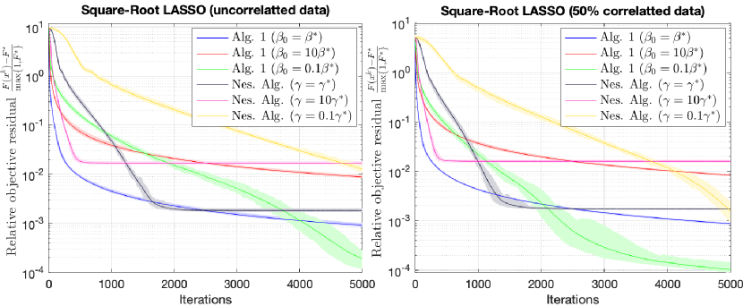
Figure 1: The convergence behavior of Algorithm 1 and Nesterov’s smoothing scheme on $30$ problem instances of (28) (the non-strongly convex case). Left plot: uncorrelated columns in $K$, and Right plot: $50\%$ correlated columns in $K$.

From Figure 1, we can observe that, with the choice $\beta_{0}:=\beta^{*}$ and $\gamma:=\gamma^{*}$ as suggested by the theory, both algorithms perform best compared to other smaller or larger values of these parameters. We also see that Algorithm 1 outperforms Nesterov’s smoothing scheme in both experiments. If $\beta_{0}$ (respectively, $\gamma$) is large, then both algorithms make good progress in early iterations, but become saturated at a given objective value in the last iterations. Alternatively, if $\beta_{0}$ (respectively, $\gamma$) is small, then both algorithms perform worse in early iterations, but further decrease the objective value when the number of iterations is increasing. This behavior also confirms the theoretical results stated in Theorem 3.1 and in Nesterov2005c . In fact, if $\beta_{0}$ (or $\gamma$) is small, then the algorithmic stepsize is small. Hence, the algorithm makes slow progress at early iterations, but it better approximates the nonsmooth function $g$, leading to more accurate approximation from $F(x^{k})$ to $F(x^{\star})$. In contrast, if $\beta_{0}$ (or $\gamma$) is large, then we have a large stepsize and therefore a faster convergence rate in early iterations. However, the smoothed approximation is less accurate.

In order to test the strongly convex case in Theorem 3.2, we conduct two additional experiments on (28) with $\rho:=0.1$. In this case, problem (28) is strongly convex with $\mu_{f}:=0.1$. Since Nesterov2005c does not directly handle the strongly convex case, we only compare two variants of Algorithm 1 stated in Theorem 3.1 (Alg. 1) and Theorem 3.2 (Alg. 1b), respectively. We set $\beta_{0}:=\frac{0.382\|K\|^{2}}{\mu_{f}}$ in Alg. 1b) as suggested by Theorem 3.2. We consider two experiments as follows:

• Experiment 3: Test two variants of Algorithm 1 on a collection of $30$ problem instances with uncorrelated columns of $K$.

• Experiment 4: Conduct the same test on another set of $30$ problem instances, but using $50\%$ correlated columns in $K$.

The results of both variants of Algorithm 1 are reported in Figure 2, where the left plot is for Experiment 3 and the right plot is for Experiment 4.

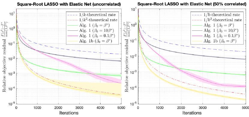
Figure 2: The convergence behavior of the two variants of Algorithm 1 on a collection of $30$ problem instances of (28) (the strongly convex case). Left plot: uncorrelated columns in $K$, and Right plot: $50\%$ correlated columns in $K$.

Clearly, as shown in Figure 2, Alg. 1b (i.e. corresponding to Theorem 3.2) highly outperforms Alg. 1 (corresponding to Theorem 3.1). Alg. 1 matches well the $\mathcal{O}\left(1/k\right)$ convergence rate as stated in Theorem 3.1, while Alg. 1b shows its $\mathcal{O}\left(1/k^{2}\right)$ convergence rate as indicated by Theorem 3.2. Note that since $g^{*}$ in (28) is non-strongly convex, we omit testing the result of Theorem 3.3. This case is rather well studied in the literature, see, e.g., Chambolle2011 .

5 Concluding Remarks

We have developed a new variant of ASGRD introduced in (TranDinh2015b, , Algorithm 1), Algorithm 1, that unifies three different settings: general convexity, strong convexity, and strong convexity and smoothness. We have proved the convergence of Algorithm 1 for three settings on three convergence criteria: gap function, primal objective residual, and dual objective residual. Our convergence rates in all cases are optimal up to a constant factor and the convergence rates of the primal sequence is on the last iterate. Our preliminary numerical experiments have shown that the theoretical convergence rates of Algorithm 1 match well the actual rates observed in practice. The proposed algorithm can be easily extended to solve composite convex problems with three or multi-objective terms. It can also be customized to solve other models, including general linear and nonlinear constrained convex problems as discussed in sabach2020faster ; TranDinh2015b ; tran2019non .

Acknowledgments. This work is partly supported by the Office of Naval Research under Grant No. ONR-N00014-20-1-2088 (2020 - 2023), and the Nafosted Vietnam, Grant No. 101.01-2020.06 (2020 - 2022).

Appendix A Appendix 1: Technical Lemmas

We need the following technical lemmas for our convergence analysis in the main text.

Lemma 4

$($(TranDinh2015b, , Lemma 10)$)$ Given $\beta>0$, $\dot{y}\in\mathbb{R}^{n}$, and a proper, closed, and convex function $g:\mathbb{R}^{n}\to\mathbb{R}\cup\{+\infty\}$ with its Fenchel conjugate $g^{*}$, we define

$$g_{\beta}(u,\dot{y}):=\max_{y\in\mathbb{R}^{n}}\left\{\langle u,y\rangle-g^{*}(y)-\tfrac{\beta}{2}\|y-\dot{y}\|^{2}\right\}.$$ (29)

Let $y^{*}_{\beta}(u,\dot{y})$ be the unique solution of (29). Then, the following statements hold:

• $g_{\beta}(\cdot,\dot{y})$ is convex w.r.t. $u$ on $\mathrm{dom}\left(g\right)$ and $\frac{1}{\beta+\mu_{g^{*}}}$-smooth w.r.t. $u$ on $\mathrm{dom}\left(g\right)$, where $\nabla_{u}{g_{\beta}}(u,\dot{y})=\textrm{prox}_{g^{*}/\beta}(\dot{y}+\frac{1}{\beta}u)$. Moreover, for any $u,\hat{u}\in\mathrm{dom}\left(g\right)$, we have

  $$g_{\beta}(\hat{u},\dot{y})+\langle\nabla{g}_{\beta}(\hat{u},\dot{y}),u-\hat{u}\rangle\leq g_{\beta}(u,\dot{y})-\frac{\beta+\mu_{g^{*}}}{2}\|\nabla_{u}{g_{\beta}}(\hat{u},\dot{y})-\nabla_{u}{g_{\beta}}(u,\dot{y})\|^{2}.$$ (30)

• For any $\beta>0$, $\dot{y}\in\mathbb{R}^{n}$, and $u\in\mathrm{dom}\left(g\right)$, we have

  $$\begin{array}[]{lcl}g_{\beta}(u,\dot{y})\leq g(u)\leq g_{\beta}(u,\dot{y})+\frac{\beta}{2}[D_{g}(\dot{y})]^{2},\ \text{where}\ D_{g}(\dot{y}):=\sup_{y\in\partial{g(u)}}\left\|y-\dot{y}\right\|.\end{array}$$ (31)

• For $u\in\mathrm{dom}\left(g\right)$ and $\dot{y}\in\mathbb{R}^{n}$, $g_{\beta}(u,\dot{y})$ is convex in $\beta$, and for all $\hat{\beta}\geq\beta>0$, we have

  $$g_{\beta}(u,\dot{y})\leq g_{\hat{\beta}}(u,\dot{y})+\big{(}\tfrac{\hat{\beta}-\beta}{2}\big{)}\|\nabla_{u}{g_{\beta}}(u,\dot{y})-\dot{y}\|^{2}.$$ (32)

• For any $\beta>0$, and $u,\hat{u}\in\mathrm{dom}\left(g\right)$, we have

  $$\hskip 21.52771pt\begin{array}[]{lcl}g_{\beta}(u,\dot{y})+\langle\nabla_{u}{g_{\beta}}(u,\dot{y}),\hat{u}-u\rangle&\leq&\ell_{\beta}(\hat{u},\dot{y})-\frac{\beta}{2}\|\nabla_{u}{g_{\beta}}(u,\dot{y})-\dot{y}\|^{2},\end{array}$$ (33)

  where $\ell_{\beta}(\hat{u},\dot{y}):=\langle\hat{u},\nabla_{u}{g_{\beta}}(u,\dot{y})\rangle-g^{*}(\nabla_{u}{g_{\beta}}(u,\dot{y}))\leq g(\hat{u})-\frac{\mu_{g^{*}}}{2}\|\nabla_{u}{g_{\beta}}(u,\dot{y})-\nabla{g}(\hat{u})\|^{2}$ for any $\nabla{g}(\hat{u})\in\partial{g}(\hat{u})$.

Lemma 5

The following statements hold.

• Let $\left\{\tau_{k}\right\}\subset(0,1]$ be computed by $\tau_{k+1}:=\frac{\tau_{k}}{2}\big{[}(\tau_{k}^{2}+4)^{1/2}-\tau_{k}\big{]}$ for some $\tau_{0}\in(0,1]$. Then, we have

  $$\tau_{k}^{2}=(1-\tau_{k})\tau_{k-1}^{2},\quad\frac{1}{k+1/\tau_{0}}\leq\tau_{k}<\frac{2}{k+2/\tau_{0}},\quad\text{and}\quad\frac{1}{1+\tau_{k-2}}\leq 1-\tau_{k}\leq\frac{1}{1+\tau_{k-1}}.$$

  Moreover, we also have

  $$\begin{array}[]{ll}&\Theta_{l,k}:=\displaystyle\prod_{i=l}^{k}(1-\tau_{i})=\dfrac{\tau_{k}^{2}}{\tau_{l-1}^{2}}\quad\text{for}\ 0\leq l\leq k,\qquad\Theta_{0,k}=\dfrac{(1-\tau_{0})\tau_{k}^{2}}{\tau_{0}^{2}}\leq\dfrac{4(1-\tau_{0})}{(\tau_{0}k+2)^{2}},\vspace{1ex}\\ \text{and}&\dfrac{\tau_{l+1}^{2}}{\tau_{k+2}^{2}}\leq\Gamma_{l,k}:=\displaystyle\prod_{i=l}^{k}(1+\tau_{i})\leq\dfrac{\tau_{l}^{2}}{\tau_{k+1}^{2}}\quad\text{for}\ 0\leq l\leq k.\end{array}$$

  If we update $\beta_{k}:=\frac{\beta_{k-1}}{1+\tau_{k}}$ for a given $\beta_{0}>0$, then

  $$\frac{4\beta_{0}\tau_{0}^{2}}{\tau_{1}^{2}[\tau_{0}(k+1)+2]^{2}}\leq\frac{\beta_{0}\tau_{k+1}^{2}}{\tau_{1}^{2}}\leq\beta_{k}=\frac{\beta_{0}}{\Gamma_{1,k}}\leq\frac{\beta_{0}\tau_{k+2}^{2}}{\tau_{2}^{2}}\leq\frac{4\beta_{0}\tau_{0}^{2}}{\tau_{2}^{2}[\tau_{0}(k+2)+2]^{2}}.$$

• Let $\left\{\tau_{k}\right\}\subset(0,1]$ be computed by solving $\tau_{k}^{3}+\tau_{k}^{2}+\tau_{k-1}^{2}\tau_{k}-\tau_{k-1}^{2}=0$ for all $k\geq 1$ and $\tau_{0}:=1$. Then, we have $\frac{1}{k+1}\leq\tau_{k}\leq\frac{2}{k+2}$ and $\Theta_{1,k}:=\prod_{i=1}^{k}(1-\tau_{i})\leq\frac{1}{k+1}$. Moreover, if we update $\beta_{k}:=\frac{\beta_{k-1}}{1+\tau_{k}}$, then $\beta_{k}\leq\frac{2\beta_{0}}{k+2}$.

Proof

The first two relations of (a) have been proved, e.g., in TranDinh2012a . Let us prove the last inequality of (a). Since $\frac{1}{1+\tau_{k-2}}\leq 1-\tau_{k}$ is equivalent to $\tau_{k-2}(1-\tau_{k})\geq\tau_{k}$. Using $1-\tau_{k}=\frac{\tau_{k}^{2}}{\tau_{k-1}^{2}}$, we have $\tau_{k}\tau_{k-2}\geq\tau_{k-1}^{2}$. Utilizing $\tau_{k}=\frac{\tau_{k-1}}{2}\big{[}(\tau_{k-1}^{2}+4)^{2}-\tau_{k-1}\big{]}$, this condition is equivalent to $\tau_{k-2}^{2}\geq\tau_{k-1}^{2}(1+\tau_{k-2})$. However, since $\tau_{k-1}^{2}=(1-\tau_{k-1})\tau_{k-2}^{2}$, the last condition becomes $1\geq(1-\tau_{k-1})(1+\tau_{k-2})$, or equivalently, $\tau_{k-1}\leq\tau_{k-2}$, which automatically holds.

To prove $1-\tau_{k}\leq\frac{1}{1+\tau_{k-1}}$, we write it as $\tau_{k-1}(1-\tau_{k})\leq\tau_{k}$. Using again $\tau_{k}^{2}=(1-\tau_{k})\tau_{k-1}^{2}$, the last inequality is equivalent to $\tau_{k}\leq\tau_{k-1}$, which automatically holds. The last statements of (a) is a consequence of $1-\tau_{k}=\frac{\tau_{k}^{2}}{\tau_{k-1}^{2}}$ and the previous relations.

(b) We consider the function $\varphi(\tau):=\tau^{3}+\tau^{2}+\tau_{k-1}^{2}\tau-\tau_{k-1}^{2}$. Clearly, $\varphi(0)=-\tau_{k-1}^{2}<0$ and $\varphi(1)=2>0$. Moreover, $\varphi^{\prime}(\tau)=3\tau^{2}+2\tau+\tau_{k-1}^{2}>0$ for $\tau\in[0,1]$. Hence, the cubic equation $\varphi(\tau)=0$ has a unique solution $\tau_{k}\in(0,1)$. Therefore, $\{\tau_{k}\}_{k\geq 0}$ is well-defined.

Next, since $\tau_{k}^{3}+\tau_{k}^{2}+\tau_{k}\tau_{k-1}^{2}-\tau_{k-1}^{2}=0$ is equivalent to $\tau_{k-1}^{2}(1-\tau_{k})=\tau_{k}^{2}(1+\tau_{k})$, we have $\tau_{k-1}^{2}(1-\tau_{k})=\tau_{k}^{2}(1+\tau_{k})\leq\frac{\tau_{k}^{2}}{1-\tau_{k}}$. This inequality becomes $\tau_{k}\geq\frac{\tau_{k-1}}{1+\tau_{k-1}}$. By induction and $\tau_{0}=1$, we can easily show that $\tau_{k}\geq\frac{1}{k+1}$. On the other hand, $\tau_{k-1}^{2}(1-\tau_{k})=\tau_{k}^{2}(1+\tau_{k})\geq\tau_{k}^{2}$. From this inequality, with a similar argument as in the proof of the statement (a), we can also easily show that $\tau_{k}\leq\frac{2}{k+2}$. Hence, we have $\frac{1}{k+1}\leq\tau_{k}\leq\frac{2}{k+2}$ for all $k\geq 0$.

Finally, since $\tau_{k}\geq\frac{1}{k+1}$, we have $\prod_{i=1}^{k}(1-\tau_{i})\leq\prod_{i=1}^{k}\left(1-\frac{1}{i+1}\right)=\frac{1}{k+1}$. Alternatively, $\prod_{i=1}^{k}(1+\tau_{i})\geq\prod_{i=1}^{k}\left(1+\frac{1}{i+1}\right)=\frac{k+2}{2}$. However, since $\beta_{k}=\frac{\beta_{k-1}}{1+\tau_{k}}$, we have $\beta_{k}=\beta_{0}\prod_{i=1}^{k}\frac{1}{1+\tau_{i}}\leq\frac{2\beta_{0}}{k+2}$. $\square$

Lemma 6

$($(ZhuLiuTran2020, , Lemma 4) and TranDinh2015b $)$ The following statements hold.

• For any $u,v,w\in\mathbb{R}^{p}$ and $t_{1},t_{2}\in\mathbb{R}$ such that $t_{1}+t_{2}\neq 0$, we have

  $$t_{1}\|u-w\|^{2}+t_{2}\|v-w\|^{2}=(t_{1}+t_{2})\|w-\tfrac{1}{t_{1}+t_{2}}(t_{1}u+t_{2}v)\|^{2}+\tfrac{t_{1}t_{2}}{t_{1}+t_{2}}\|u-v\|^{2}.$$

• For any $\tau\in(0,1)$, $\hat{\beta},\beta>0$, $w,z\in\mathbb{R}^{p}$, we have

  $$\begin{array}[]{lcl}\beta(1-\tau)\|w-z\|^{2}+\beta\tau\|w\|^{2}-(1-\tau)(\hat{\beta}-\beta)\|z\|^{2}&=&\beta\|w-(1-\tau)z\|^{2}\vspace{1ex}\\ &&+{~{}}(1-\tau)\big{[}\tau\beta-(\hat{\beta}-\beta)\big{]}\|z\|^{2}.\end{array}$$

The following lemma is a key step to address the strongly convex case of $f$ in (1).

Lemma 7

Given $L_{k}>0$, $\mu_{f}>0$, and $\tau_{k}\in(0,1)$, let $m_{k}:=\frac{L_{k}+\mu_{f}}{L_{k-1}+\mu_{f}}$ and $a_{k}:=\frac{L_{k}}{L_{k-1}+\mu_{f}}$. Assume that the following two conditions hold:

$$\left\{\begin{array}[]{llcl}&(1-\tau_{k})\big{[}\tau_{k-1}^{2}+m_{k}\tau_{k}\big{]}&\geq&a_{k}\tau_{k}\vspace{1ex}\\ &m_{k}\tau_{k}\tau_{k-1}^{2}+m_{k}^{2}\tau_{k}^{2}&\geq&a_{k}\tau_{k-1}^{2}.\end{array}\right.$$ (34)

Let $\left\{x^{k}\right\}$ be a given sequence in $\mathbb{R}^{p}$. We define $\hat{x}^{k}:=x^{k}+\frac{1}{\omega_{k}}(x^{k}-x^{k-1})$, where $\omega_{k}$ is chosen such that

$$\max\left\{\frac{\tau_{k-1}+\sqrt{\tau_{k-1}^{2}+4a_{k}}}{2(1-\tau_{k-1})},\frac{a_{k}\tau_{k}}{(1-\tau_{k})(1-\tau_{k-1})\tau_{k-1}}\right\}\leq\omega_{k}\leq\frac{\tau_{k-1}^{2}+m_{k}\tau_{k}}{\tau_{k-1}(1-\tau_{k-1})}.$$ (35)

Then, $\omega_{k}$ is well-defined, and for any $x\in\mathbb{R}^{p}$, we have

$$\begin{array}[]{ll}&L_{k}\tau_{k}^{2}\|\frac{1}{\tau_{k}}[\hat{x}^{k}-(1-\tau_{k})x^{k}]-x\|^{2}-\mu_{f}\tau_{k}(1-\tau_{k})\|x^{k}-x\|^{2}\vspace{1ex}\\ &\qquad\leq{~{}}(1-\tau_{k})\left(L_{k-1}+\mu_{f}\right)\tau_{k-1}^{2}\|\frac{1}{\tau_{k-1}}[x^{k}-(1-\tau_{k-1})x^{k-1}]-x\|^{2}.\end{array}$$ (36)

Proof

Firstly, from the definition $\hat{x}^{k}:=x^{k}+\frac{1}{\omega_{k}}(x^{k}-x^{k-1})$ of $\hat{x}^{k}$, we have $\omega_{k}(\hat{x}^{k}-x^{k})=x^{k}-x^{k-1}$. Hence, we can show that

$$\begin{array}[]{lcl}\tau_{k-1}^{2}\|\frac{1}{\tau_{k-1}}[x^{k}-(1-\tau_{k-1})x^{k-1}]-x\|^{2}&=&\|(1-\tau_{k-1})(x^{k}-x^{k-1})+\tau_{k-1}(x^{k}-x)\|^{2}\vspace{1ex}\\ &=&\|(1-\tau_{k-1})\omega_{k}(\hat{x}^{k}-x^{k})+\tau_{k-1}(x^{k}-x)\|^{2}\vspace{1ex}\\ &=&\omega_{k}^{2}(1-\tau_{k-1})^{2}\|\hat{x}^{k}-x^{k}\|^{2}+\tau_{k-1}^{2}\|x^{k}-x\|^{2}\vspace{1ex}\\ &&+{~{}}2\omega_{k}(1-\tau_{k-1})\tau_{k-1}\langle\hat{x}^{k}-x^{k},x^{k}-x\rangle.\end{array}$$

Alternatively, we also have

$$\begin{array}[]{lcl}\tau_{k}^{2}\|\frac{1}{\tau_{k}}[\hat{x}^{k}-(1-\tau_{k})x^{k}]-x\|^{2}&=&\|\hat{x}^{k}-x^{k}\|^{2}+\tau_{k}^{2}\|x^{k}-x\|^{2}+2\tau_{k}\langle\hat{x}^{k}-x^{k},x^{k}-x\rangle.\end{array}$$

Utilizing the two last expressions, (36) can be rewritten equivalently to

$$\begin{array}[]{lcl}\mathcal{T}_{[1]}&:=&2\left[\left(L_{k-1}+\mu_{f}\right)(1-\tau_{k})(1-\tau_{k-1})\tau_{k-1}\omega_{k}-L_{k}\tau_{k}\right]\langle\hat{x}^{k}-x^{k},x-x^{k}\rangle\vspace{1ex}\\ &\leq&\left[\left(L_{k-1}+\mu_{f}\right)(1-\tau_{k})(1-\tau_{k-1})^{2}\omega_{k}^{2}-L_{k}\right]\|\hat{x}^{k}-x^{k}\|^{2}\vspace{1ex}\\ &&+{~{}}\left[\left(L_{k-1}+\mu_{f}\right)(1-\tau_{k})\tau_{k-1}^{2}-L_{k}\tau_{k}^{2}+\mu_{f}\tau_{k}(1-\tau_{k})\right]\|x^{k}-x\|^{2}.\end{array}$$

Now, let us denote

$$\left\{\begin{array}[]{lcl}c_{1}&:=&\left(L_{k-1}+\mu_{f}\right)(1-\tau_{k})(1-\tau_{k-1})\tau_{k-1}\omega_{k}-L_{k}\tau_{k}\vspace{1ex}\\ c_{2}&:=&\left(L_{k-1}+\mu_{f}\right)(1-\tau_{k})(1-\tau_{k-1})^{2}\omega_{k}^{2}-L_{k}\vspace{1ex}\\ c_{3}&:=&\left(L_{k-1}+\mu_{f}\right)(1-\tau_{k})\tau_{k-1}^{2}-L_{k}\tau_{k}^{2}+\mu_{f}(1-\tau_{k})\tau_{k}.\end{array}\right.$$

Then, (36) is equivalent to

$$2c_{1}\langle\hat{x}^{k}-x^{k},x-x^{k}\rangle\leq c_{2}\|\hat{x}^{k}-x^{k}\|^{2}+c_{3}\|x-x^{k}\|^{2}.$$ (37)

Secondly, we need to guarantee that $c_{1}\geq 0$. This condition holds if we choose $\omega_{k}$ such that

$$\omega_{k}\geq\frac{a_{k}\tau_{k}}{(1-\tau_{k})(1-\tau_{k-1})\tau_{k-1}}.$$ (38)

Thirdly, we also need to guarantee $c_{2}\geq c_{1}$, which is equivalent to

$$c_{2}-c_{1}=\left(L_{k-1}+\mu_{f}\right)(1-\tau_{k})(1-\tau_{k-1})\left[(1-\tau_{k-1})\omega_{k}^{2}-\tau_{k-1}\omega_{k}\right]-L_{k}(1-\tau_{k})\geq 0.$$

This condition holds if

$$\omega_{k}\geq\frac{\tau_{k-1}+\sqrt{\tau_{k-1}^{2}+4a_{k}}}{2(1-\tau_{k-1})}.$$ (39)

Alternatively, we also need to guarantee $c_{3}\geq c_{1}$, which is equivalent to

$$c_{3}-c_{1}=\left(L_{k-1}+\mu_{f}\right)(1-\tau_{k})\left[\tau_{k-1}^{2}-(1-\tau_{k-1})\tau_{k-1}\omega_{k}\right]+(L_{k}+\mu_{f})\tau_{k}(1-\tau_{k})\geq 0.$$

This condition holds if

$$\omega_{k}\leq\frac{\tau_{k-1}^{2}+m_{k}\tau_{k}}{\tau_{k-1}(1-\tau_{k-1})}.$$ (40)

Combining (38), (39), and (40), we obtain

$$\max\left\{\frac{\tau_{k-1}+\sqrt{\tau_{k-1}^{2}+4a_{k}}}{2(1-\tau_{k-1})},\frac{a_{k}\tau_{k}}{(1-\tau_{k})(1-\tau_{k-1})\tau_{k-1}}\right\}\leq\omega_{k}\leq\frac{\tau_{k-1}^{2}+m_{k}\tau_{k}}{\tau_{k-1}(1-\tau_{k-1})},$$

which is exactly (35). Here, under the condition (34), the left-hand side of the last expression is less than or equal to the right-hand side. Therefore, $\omega_{k}$ is well-defined.

Finally, under the choice of $\omega_{k}$ as in (35), we have $c_{2}\geq c_{1}\geq 0$ and $c_{3}\geq c_{1}\geq 0$. Hence, (37) holds, which is also equivalent to (36). $\square$

Appendix B Appendix 2: Technical Proof of Lemmas 2 and 3 in Section 3

This section provides the full proof of Lemma 2 and Lemma 3 in the main text.

B.1 The proof of Lemma 2: Key estimate of the primal-dual step (9)

Proof

From the first line of (9) and Lemma 4(a), we have $\nabla_{u}g_{\beta_{k}}(K\hat{x}^{k},\dot{y})=K^{\top}y^{k+1}$. Now, from the second line of (9), we also have

$$0\in\partial{f}(x^{k+1})+L_{k}(x^{k+1}-\hat{x}^{k})+K^{\top}\nabla_{u}{g_{\beta_{k}}}(K\hat{x}^{k},\dot{y}).$$

Combining this inclusion and the $\mu_{f}$-convexity of $f$, for any $x\in\mathrm{dom}\left(f\right)$, we get

$$\begin{array}[]{lcl}f(x^{k+1})&\leq&f(x)+\langle\nabla_{u}{g_{\beta_{k}}}(K\hat{x}^{k},\dot{y}),K(x-x^{k+1})\rangle+L_{k}\langle x^{k+1}-\hat{x}^{k},x-x^{k+1}\rangle\vspace{1ex}\\ &&-{~{}}\frac{\mu_{f}}{2}\|x^{k+1}-x\|^{2}.\end{array}$$

Since $g_{\beta}(\cdot,\dot{y})$ is $\frac{1}{\beta+\mu_{g^{*}}}$-smooth by Lemma 4(a), for any $x\in\mathrm{dom}\left(f\right)$, we have

$$\begin{array}[]{lcl}g_{\beta_{k}}(Kx^{k+1},\dot{y})&\leq&g_{\beta_{k}}(K\hat{x}^{k},\dot{y})+\langle\nabla_{u}{g}_{\beta_{k}}(K\hat{x}^{k},\dot{y}),K(x^{k+1}-\hat{x}^{k})\rangle\vspace{1ex}\\ &&+{~{}}\frac{1}{2(\beta_{k}+\mu_{g^{*}})}\|K(x^{k+1}-\hat{x}^{k})\|^{2}\vspace{1ex}\\ &=&g_{\beta_{k}}(K\hat{x}^{k},\dot{y})+\langle\nabla_{u}g_{\beta_{k}}(K\hat{x}^{k},\dot{y}),K(x-\hat{x}^{k})\rangle\vspace{1ex}\\ &&-{~{}}\langle\nabla_{u}{g}_{\beta_{k}}(K\hat{x}^{k},\dot{y}),K(x-x^{k+1})\rangle\vspace{1ex}\\ &&+{~{}}\frac{1}{2(\mu_{g^{*}}+\beta_{k})}\|K(x^{k+1}-\hat{x}^{k})\|^{2}.\end{array}$$

Now, combining the last two estimates, we get

$$\begin{array}[]{lcl}f(x^{k+1})+g_{\beta_{k}}(Kx^{k+1},\dot{y})&\leq&f(x)+g_{\beta_{k}}(K\hat{x}^{k},\dot{y})+\langle\nabla_{u}g_{\beta_{k}}(K\hat{x}^{k},\dot{y}),K(x-\hat{x}^{k})\rangle\vspace{1ex}\\ &&+{~{}}L_{k}\langle x^{k+1}-\hat{x}^{k},x-\hat{x}^{k}\rangle-L_{k}\|x^{k+1}-\hat{x}^{k}\|^{2}\vspace{1ex}\\ &&+{~{}}\frac{1}{2(\mu_{g^{*}}+\beta_{k})}\|K(x^{k+1}-\hat{x}^{k})\|^{2}-\frac{\mu_{f}}{2}\|x-x^{k+1}\|^{2}.\end{array}$$ (41)

Using Lemma 4(a) again, we have

$$\begin{array}[]{lcl}\ell_{\beta_{k}}(x^{k},\dot{y})&:=&g_{\beta_{k}}(K\hat{x}^{k},\dot{y})+\langle\nabla_{u}g_{\beta_{k}}(K\hat{x}^{k},\dot{y}),K(x^{k}-\hat{x}^{k})\rangle\vspace{1ex}\\ &\leq&g_{\beta_{k}}(Kx^{k},\dot{y})-\frac{\beta_{k}+\mu_{g^{*}}}{2}\|\nabla_{u}g_{\beta_{k}}(K\hat{x}^{k},\dot{y})-\nabla_{u}g_{\beta_{k}}(Kx^{k},\dot{y})\|^{2}.\end{array}$$ (42)

Substituting $x:=x^{k}$ into (41), and multiplying the result by $1-\tau_{k}$ and adding the result to (41) after multiplying it by $\tau_{k}$, then using (42), we can derive

$$\begin{array}[]{lcl}F_{\beta_{k}}(x^{k+1},\dot{y})&:=&f(x^{k+1})+g_{\beta_{k}}(Kx^{k+1},\dot{y})\vspace{1ex}\\ &\leq&(1-\tau_{k})[f(x^{k})+g_{\beta_{k}}(Kx^{k},\dot{y})]+\tau_{k}\left[f(x)+\ell_{\beta_{k}}(x,\dot{y})\right]\vspace{1ex}\\ &&-{~{}}L_{k}\|x^{k+1}-\hat{x}^{k}\|^{2}+\frac{1}{2(\mu_{g^{*}}+\beta_{k})}\|K(x^{k+1}-\hat{x}^{k})\|^{2}\vspace{1ex}\\ &&+{~{}}L_{k}\langle x^{k+1}-\hat{x}^{k},\tau_{k}x-\hat{x}^{k}+(1-\tau_{k})x^{k}\rangle\vspace{1ex}\\ &&-{~{}}\frac{\mu_{f}}{2}\left[(1-\tau_{k})\|x^{k+1}-x^{k}\|^{2}+\tau_{k}\|x-x^{k+1}\|^{2}\right]\vspace{1ex}\\ &&-{~{}}\frac{(1-\tau_{k})(\beta_{k}+\mu_{g^{*}})}{2}\|\nabla_{u}g_{\beta_{k}}(K\hat{x}^{k},\dot{y})-\nabla_{u}g_{\beta_{k}}(Kx^{k},\dot{y})\|^{2}.\end{array}$$ (43)

From Lemma 6(a), we can easily show that

$$\begin{array}[]{lcl}(1-\tau_{k})\|x^{k+1}-x^{k}\|^{2}+\tau_{k}\|x^{k+1}-x\|^{2}&=&\tau_{k}^{2}\|\tfrac{1}{\tau_{k}}[x^{k+1}-(1-\tau_{k})x^{k}]-x\|^{2}\vspace{1ex}\\ &&+{~{}}\tau_{k}(1-\tau_{k})\|x-x^{k}\|^{2}.\end{array}$$

We also have the following elementary relation

$$\begin{array}[]{lcl}\langle x^{k+1}-\hat{x}^{k},\tau_{k}x-[\hat{x}^{k}-(1-\tau_{k})x^{k}]\rangle&=&\frac{\tau_{k}^{2}}{2}\|\tfrac{1}{\tau_{k}}[\hat{x}^{k}-(1-\tau_{k})x^{k}]-x\|^{2}+\frac{1}{2}\|x^{k+1}-\hat{x}^{k}\|^{2}\vspace{1ex}\\ &&-{~{}}\frac{\tau_{k}^{2}}{2}\|\tfrac{1}{\tau_{k}}[x^{k+1}-(1-\tau_{k})x^{k}]-x\|^{2}.\end{array}$$

Substituting the two last expressions into (43), we obtain

$$\begin{array}[]{lcl}F_{\beta_{k}}(x^{k+1},\dot{y})&\leq&(1-\tau_{k})F_{\beta_{k}}(x^{k},\dot{y})+\tau_{k}\left[f(x)+\ell_{\beta_{k}}(x,\dot{y})\right]\vspace{1ex}\\ &&+{~{}}\frac{L_{k}\tau_{k}^{2}}{2}\|\tfrac{1}{\tau_{k}}[\hat{x}^{k}-(1-\tau_{k})x^{k}]-x\|^{2}\vspace{1ex}\\ &&-{~{}}\frac{\tau_{k}^{2}}{2}\left(L_{k}+\mu_{f}\right)\|\tfrac{1}{\tau_{k}}[x^{k+1}-(1-\tau_{k})x^{k}]-x\|^{2}\vspace{1ex}\\ &&-{~{}}\frac{(1-\tau_{k})(\mu_{g^{*}}+\beta_{k})}{2}\|\nabla_{u}g_{\beta_{k}}(K\hat{x}^{k},\dot{y})-\nabla_{u}g_{\beta_{k}}(Kx^{k},\dot{y})\|^{2}\vspace{1ex}\\ &&-{~{}}\frac{L_{k}}{2}\|x^{k+1}-\hat{x}^{k}\|^{2}+\frac{1}{2(\mu_{g^{*}}+\beta_{k})}\|K(x^{k+1}-\hat{x}^{k})\|^{2}\vspace{1ex}\\ &&-{~{}}\frac{\mu_{f}(1-\tau_{k})\tau_{k}}{2}\|x-x^{k}\|^{2}.\end{array}$$ (44)

One the one hand, by (32) of Lemma 4, we have

$$F_{\beta_{k}}(x^{k},\dot{y})\leq F_{\beta_{k-1}}(x^{k},\dot{y})+\frac{(\beta_{k-1}-\beta_{k})}{2}\|\nabla_{u}g_{\beta_{k}}(Kx^{k},\dot{y})-\dot{y}\|^{2}.$$

On the other hand, by (33) of Lemma 4, we get

$$f(x)+\ell_{\beta_{k}}(x,\dot{y})\leq\mathcal{L}(x,y^{k+1})-\frac{\beta_{k}}{2}\|\nabla_{u}g_{\beta_{k}}(K\hat{x}^{k},\dot{y})-\dot{y}\|^{2},$$

where $\mathcal{L}(x,y^{k+1}):=f(x)+\langle Kx,y^{k+1}\rangle-g^{*}(y^{k+1})$ is the Lagrange function in (1).

Now, substituting the last two inequalities into (44), and using Lemma 6(b) with $w:=\nabla_{u}g_{\beta_{k}}(K\hat{x}^{k},\dot{y})-\dot{y}$ and $z:=\nabla_{u}g_{\beta_{k}}(Kx^{k},\dot{y})-\dot{y}$, we arrive at

$$\begin{array}[]{lcl}F_{\beta_{k}}(x^{k+1},\dot{y})&\leq&(1-\tau_{k})F_{\beta_{k-1}}(x^{k},\dot{y})+\tau_{k}\mathcal{L}(x,y^{k+1})+\frac{L_{k}\tau_{k}^{2}}{2}\|\tfrac{1}{\tau_{k}}[\hat{x}^{k}-(1-\tau_{k})x^{k}]-x\|^{2}\vspace{1ex}\\ &&-{~{}}\frac{\tau_{k}^{2}}{2}\left(L_{k}+\mu_{f}\right)\|\tfrac{1}{\tau_{k}}[x^{k+1}-(1-\tau_{k})x^{k}]-x\|^{2}-\frac{\mu_{f}(1-\tau_{k})\tau_{k}}{2}\|x-x^{k}\|^{2}\vspace{1ex}\\ &&-{~{}}\frac{L_{k}}{2}\|x^{k+1}-\hat{x}^{k}\|^{2}+\frac{1}{2(\mu_{g^{*}}+\beta_{k})}\|K(x^{k+1}-\hat{x}^{k})\|^{2}\vspace{1ex}\\ &&-{~{}}\frac{(1-\tau_{k})}{2}\left[\tau_{k}\beta_{k}-(\beta_{k-1}-\beta_{k})\right]\|\nabla_{u}g_{\beta_{k}}(Kx^{k},\dot{y})-\dot{y}\|^{2}\vspace{1ex}\\ &&-{~{}}\frac{\beta_{k}}{2}\|\nabla_{u}g_{\beta_{k}}(K\hat{x}^{k},\dot{y})-\dot{y}-(1-\tau_{k})\left[\nabla_{u}g_{\beta_{k}}(Kx^{k},\dot{y})-\dot{y}\right]\|^{2}\vspace{1ex}\\ &&-{~{}}\frac{(1-\tau_{k})\mu_{g^{*}}}{2}\|\nabla_{u}g_{\beta_{k}}(K\hat{x}^{k},\dot{y})-\nabla_{u}g_{\beta_{k}}(Kx^{k},\dot{y})\|^{2}.\end{array}$$

By dropping the last two nonpositive terms in the last inequality, we obtain (10). $\square$

B.2 The proof of Lemma 3: Recursive estimate of the Lyapunov function

Proof

First, from the last line $\tilde{y}^{k+1}=(1-\tau_{k})\tilde{y}^{k}+\tau_{k}y^{k+1}$ of (11), and the $\mu_{g^{*}}$-convexity of $g^{*}$, we have

$$\begin{array}[]{lcl}\mathcal{L}(x,\tilde{y}^{k+1})&:=&f(x)+\langle Kx,\tilde{y}^{k+1}\rangle-g^{*}(\tilde{y}^{k+1})\vspace{1ex}\\ &\geq&(1-\tau_{k})\mathcal{L}(x,\tilde{y}^{k})+\tau_{k}\mathcal{L}(x,y^{k+1})+\frac{\mu_{g^{*}}\tau_{k}(1-\tau_{k})}{2}\|y^{k+1}-\tilde{y}^{k}\|^{2}.\end{array}$$

Hence, $\tau_{k}\mathcal{L}(x,y^{k+1})\leq\mathcal{L}(x,\tilde{y}^{k+1})-(1-\tau_{k})\mathcal{L}(x,\tilde{y}^{k})-\frac{\mu_{g^{*}}\tau_{k}(1-\tau_{k})}{2}\|y^{k+1}-\tilde{y}^{k}\|^{2}$. Substituting this estimate into (10) and dropping the term $-\frac{\mu_{g^{*}}\tau_{k}(1-\tau_{k})}{2}\|y^{k+1}-\tilde{y}^{k}\|^{2}$, we can derive

$$\begin{array}[]{lcl}F_{\beta_{k}}(x^{k+1},\dot{y})&\leq&(1-\tau_{k})F_{\beta_{k-1}}(x^{k},\dot{y})+\mathcal{L}(x,\tilde{y}^{k+1})-(1-\tau_{k})\mathcal{L}(x,\tilde{y}^{k})\vspace{1ex}\\ &&+{~{}}\frac{L_{k}\tau_{k}^{2}}{2}\big{\|}\tfrac{1}{\tau_{k}}[\hat{x}^{k}-(1-\tau_{k})x^{k}]-x\big{\|}^{2}\vspace{1ex}\\ &&-{~{}}\frac{\tau_{k}^{2}}{2}\left(L_{k}+\mu_{f}\right)\big{\|}\tfrac{1}{\tau_{k}}[x^{k+1}-(1-\tau_{k})x^{k}]-x\big{\|}^{2}\vspace{1ex}\\ &&-{~{}}\frac{L_{k}}{2}\|x^{k+1}-\hat{x}^{k}\|^{2}+\frac{1}{2(\mu_{g^{*}}+\beta_{k})}\|K(x^{k+1}-\hat{x}^{k})\|^{2}\vspace{1ex}\\ &&-{~{}}\frac{\mu_{f}\tau_{k}(1-\tau_{k})}{2}\|x^{k}-x\|^{2}.\end{array}$$ (45)

Now, it is obvious to show that the condition (14) is equivalent to the condition (34) of Lemma 7. In addition, we choose $\eta_{k}=\frac{1}{\omega_{k}}$ in our update (13), where $\omega_{k}:=\frac{\tau_{k-1}^{2}+m_{k}\tau_{k}}{\tau_{k-1}(1-\tau_{k-1})}$, which is the upper bound of (35). Hence, (35) automatically holds. Using (36), we have

$$\begin{array}[]{lcl}\mathcal{T}_{[2]}&:=&\frac{L_{k}\tau_{k}^{2}}{2}\big{\|}\tfrac{1}{\tau_{k}}[\hat{x}^{k}-(1-\tau_{k})x^{k}]-x\big{\|}^{2}-\frac{\mu_{f}\tau_{k}(1-\tau_{k})}{2}\|x^{k}-x\|^{2}\vspace{1ex}\\ &\leq&\frac{\tau_{k-1}^{2}}{2}(1-\tau_{k})\left(L_{k-1}+\mu_{f}\right)\big{\|}\tfrac{1}{\tau_{k-1}}[x^{k}-(1-\tau_{k-1})x^{k-1}]-x\big{\|}^{2}.\end{array}$$

Moreover, $\frac{1}{2(\mu_{g^{*}}+\beta_{k})}\|K(x^{k+1}-\hat{x}^{k})\|^{2}\leq\frac{\|K\|^{2}}{2(\mu_{g^{*}}+\beta_{k})}\|x^{k+1}-\hat{x}^{k}\|^{2}=\frac{L_{k}}{2}\|x^{k+1}-\hat{x}^{k}\|^{2}$ due to the definition of $L_{k}$ in (13). Substituting these two estimates into (45), and utilizing the definition (12) of $\mathcal{V}_{k}$, we obtain (15). $\square$

References

- [1] H. H. Bauschke and P. Combettes. Convex analysis and monotone operators theory in Hilbert spaces. Springer-Verlag, 2nd edition, 2017.
- [2] A. Beck and M. Teboulle. A fast iterative shrinkage-thresholding algorithm for linear inverse problems. SIAM J. Imaging Sci., 2(1):183–202, 2009.
- [3] A. Belloni, V. Chernozhukov, and L. Wang. Square-root LASSO: Pivotal recovery of sparse signals via conic programming. Biometrika, 94(4):791–806, 2011.
- [4] R. I. Boţ and A. Böhm. Variable smoothing for convex optimization problems using stochastic gradients. J. Sci. Comput., 85(2):1–29, 2020.
- [5] A. Chambolle and T. Pock. A first-order primal-dual algorithm for convex problems with applications to imaging. J. Math. Imaging Vis., 40(1):120–145, 2011.
- [6] A. Chambolle and T. Pock. On the ergodic convergence rates of a first-order primal–dual algorithm. Math. Program., 159(1-2):253–287, 2016.
- [7] Y. Chen, G. Lan, and Y. Ouyang. Optimal primal-dual methods for a class of saddle-point problems. SIAM J. Optim., 24(4):1779–1814, 2014.
- [8] L. Condat. A primal-dual splitting method for convex optimization involving Lipschitzian, proximable and linear composite terms. J. Optim. Theory Appl., 158:460–479, 2013.
- [9] D. Davis. Convergence rate analysis of primal-dual splitting schemes. SIAM J. Optim., 25(3):1912–1943, 2015.
- [10] D. Davis and W. Yin. A three-operator splitting scheme and its optimization applications. Set-valued and Variational Analysis, 25(4):829–858, 2017.
- [11] E. Esser, X. Zhang, and T. Chan. A general framework for a class of first order primal-dual algorithms for TV-minimization. SIAM J. Imaging Sci., 3(4):1015–1046, 2010.
- [12] T. Goldstein, E. Esser, and R. Baraniuk. Adaptive primal-dual hybrid gradient methods for saddle point problems. Tech. Report., pages 1–26, 2013. http://arxiv.org/pdf/1305.0546v1.pdf.
- [13] M. Grant. Disciplined Convex Programming. PhD thesis, Stanford University, 2004.
- [14] B. S. He and X. M. Yuan. On the convergence rate of the Douglas-Rachford alternating direction method. SIAM J. Numer. Anal., 50:700–709, 2012.
- [15] A. Nemirovskii and D. Yudin. Problem Complexity and Method Efficiency in Optimization. Wiley Interscience, 1983.
- [16] Y. Nesterov. Introductory lectures on convex optimization: A basic course, volume 87 of Applied Optimization. Kluwer Academic Publishers, 2004.
- [17] Y. Nesterov. Smooth minimization of non-smooth functions. Math. Program., 103(1):127–152, 2005.
- [18] Y. Nesterov. Gradient methods for minimizing composite objective function. Math. Program., 140(1):125–161, 2013.
- [19] D. O’Connor and L. Vandenberghe. Primal-dual decomposition by operator splitting and applications to image deblurring. SIAM J. Imaging Sci., 7(3):1724–1754, 2014.
- [20] Y. Ouyang and Y. Xu. Lower complexity bounds of first-order methods for convex-concave bilinear saddle-point problems. Math. Program., online first:1–35, 2019.
- [21] S. Sabach and M. Teboulle. Faster Lagrangian-based methods in convex optimization. arXiv preprint arXiv:2010.14314, 2020.
- [22] Q. Tran-Dinh, A. Alacaoglu, O. Fercoq, and V. Cevher. An Adaptive Primal-Dual Framework for Nonsmooth Convex Minimization. Math. Program. Compt., 12:451–491, 2020.
- [23] Q. Tran-Dinh, O. Fercoq, and V. Cevher. A smooth primal-dual optimization framework for nonsmooth composite convex minimization. SIAM J. Optim., 28(1):96–134, 2018.
- [24] Q. Tran-Dinh, C. Savorgnan, and M. Diehl. Combining Lagrangian decomposition and excessive gap smoothing technique for solving large-scale separable convex optimization problems. Compt. Optim. Appl., 55(1):75–111, 2013.
- [25] Q. Tran-Dinh and Y. Zhu. Non-stationary first-order primal-dual algorithms with faster convergence rates. SIAM J. Optim., 30(4):2866–2896, 2020.
- [26] P. Tseng. On accelerated proximal gradient methods for convex-concave optimization. Submitted to SIAM J. Optim., 2008.
- [27] T. Valkonen. Inertial, corrected, primal–dual proximal splitting. SIAM J. Optim., 30(2):1391–1420, 2020.
- [28] B. C. Vu. A variable metric extension of the forward–backward–forward algorithm for monotone operators. Numer. Funct. Anal. Optim., 34(9):1050–1065, 2013.
- [29] Y. Zhu, D. Liu, and Q. Tran-Dinh. Primal-dual algorithms for a class of nonlinear compositional convex optimization problems. arXiv preprint arXiv:2006.09263, pages 1–26, 2020.
- [30] H. Zou and T. Hastie. Regularization and variable selection via the elastic net. Journal of the Royal Statistical Society: Series B, 67(2):301–320, 2005.