1264 \vgtccategoryResearch \vgtcpapertypeapplication/design study \authorfooter
Daisen: A Framework for Visualizing Detailed GPU Execution
Abstract
Graphics Processing Units (GPUs) have been widely used to accelerate artificial intelligence, physics simulation, medical imaging, and information visualization applications. In order to improve GPU performance, GPU hardware designers need to identify performance issues by inspecting huge volumes of traces generated from simulators. Visualizing the execution traces can reduce the cognitive burden of users and facilitate making sense of behaviors of GPU hardware components. Existing visualization tools for examining GPU execution traces have primarily focused on GPU hardware components supported by specific simulators; thus were not generally applicable and cannot be easily adapted to evaluate other GPU hardware components. In this work, we first formalize the process of GPU performance analysis and characterize the design requirements of visualizing execution traces based on a survey study and informal interviews with GPU hardware designers. We contribute data and task abstraction for GPU performance analysis. Based on our task analysis, we propose Daisen, a framework that supports data collection from GPU simulators and provides visualization of the simulator-generated GPU execution traces. Daisen features generic and versatile data abstraction that can collect data from a wide range of GPU simulators and can represent the behavior of a wide variety of GPU hardware components. Daisen also includes a web-based visualization tool that helps GPU hardware designers examine GPU execution traces, identify performance bottlenecks, and verify performance improvement. Our qualitative evaluation with GPU hardware designers demonstrates that the design of Daisen reflects the typical workflow of GPU hardware designers. Participants were able to effectively identify potential performance bottlenecks and opportunities for performance improvement. Supplementary materials including the source code, a demo video, survey questions, evaluation study guide, and post-study evaluation survey are available at https://osf.io/nxd83/?view_only=48d3e7a47511447c8a0a4f241b273884.
keywords:
Performance visualization, computer architecture, simulators, program execution, GPUK.6.1Management of Computing and Information SystemsProject and People ManagementLife Cycle;
\CCScatK.7.mThe Computing ProfessionMiscellaneousEthics
\teaser
![[Uncaptioned image]](/html/2104.00828/assets/x1.png) Daisen provides a web-based interactive visualization tool that enables the examination of GPU execution traces.
(A) The Overview Panel shows key performance metrics against time of all hardware components using small multiples,
(B) the Task View demonstrates the hierarchical relationships between tasks,
(C) the Component View displays all the tasks executed in a hardware component (after selecting one component of interest from the Overview), and
(D) the legend bar shows all the tasks involved in the Component View and the Task View with color encoded.
Note that the labels ABCD do not appear on the visualization interface.
\vgtcinsertpkg
Daisen provides a web-based interactive visualization tool that enables the examination of GPU execution traces.
(A) The Overview Panel shows key performance metrics against time of all hardware components using small multiples,
(B) the Task View demonstrates the hierarchical relationships between tasks,
(C) the Component View displays all the tasks executed in a hardware component (after selecting one component of interest from the Overview), and
(D) the legend bar shows all the tasks involved in the Component View and the Task View with color encoded.
Note that the labels ABCD do not appear on the visualization interface.
\vgtcinsertpkg
Introduction
Graphics Processing Units (GPUs) were originally designed to accelerate 3D graphics rendering (e.g., 3D games, product design, animated film making). In the last decade, developers have found additional general-purpose use cases that take advantage of GPU’s architectures. Developers have been using GPUs to accelerate a wide range of applications that require high performance, including large-scale physics simulation [navarro_hitschfeld-kahler_mateu_2014], medical imaging [yan2008fast], data visualization [McDonnelElmvvist], artificial intelligence [oh2004gpu], and Blockchain hashing [morishima2018accelerating]. A GPU is capable of performing thousands of calculations in parallel. Empirical studies have demonstrated how a GPU’s massive parallel processing capabilities can speed up algorithms by 5-70X as compared to CPU implementations [AroraManish2012RtRo]. Moreover, recent developments in the features supported on the GPU computing enable it to be used to accelerate a rapidly growing range of applications, made possible through continuous improvements to performance [sun2019summarizing].
One of the ultimate goals for GPU hardware designers is to improve the design of a GPU to run applications within a shorter amount of time. Prior to implementing a new design on real hardware and sending the design to fabrication, simulations of the proposed design must be carried out extensively. Simulation allows hardware designers to compare the performance of the proposed hardware design with a baseline design over a wide range of benchmarks (i.e., standard and representative applications) [gpgpusim, multi2sim, sun2019mgpusim]. In general, it is challenging to identify and make sense of any performance bottlenecks encountered, since this may involve the designer manually inspecting gigabytes (GBs) of simulator-generated GPU-execution traces (i.e., a highly detailed record of events that occur during GPU program execution) [M2S-Visual]. Given the complexity and the massive scale of the execution trace data, visualizations are useful to help guide GPU hardware designers inspect execution state and identify potential performance issues, greatly improving the efficiency of the GPU hardware design process [aerialvision].
Prior work has described visualization systems that examine GPU execution traces, such as AerialVision [aerialvision] and M2S-Visual [M2S-Visual]. These tools have been developed for specific simulators and cannot be easily applied to other simulators. Moreover, existing tools provide specific views for each feature (e.g., instruction execution, cache access) for GPU program execution. A new view needs to be added for every new feature developed in the simulator, adding extra burden to visualization tool developers. Therefore, the GPU architecture research community needs a new visualization framework that can be easily applied to a wide range of simulators and support various visualization tasks required by researchers.
In this work, we introduce Daisen, a framework that helps GPU hardware designers collect and visualize GPU execution traces. In particular, we contribute:
-
•
A detailed task analysis and task abstraction for analyzing GPU performance. To the best of our knowledge, there is no formal study that examines the design requirements of GPU execution trace visualization to facilitate GPU hardware design. To fill this gap, we conducted a survey and informal interviews with domain experts to characterize best practices and workflows common in GPU performance analysis. Based on the survey responses with 37 GPU hardware designers, we summarize the GPU performance analysis process using a hierarchical task abstraction [zhang2019idmvis]. We identify four functional requirements and two non-functional requirements, resulting in a visualization tool more adequately suited to facilitate the performance analysis task.
-
•
A versatile and universal data abstraction that supports data collection from most GPU simulators and representation of the behavior of a wide range of digital circuit components.
-
•
The design and the implementation of a web-based visualization tool that visualizes massively-parallel GPU execution traces. Our tool aims to help GPU hardware designers identify performance bottlenecks, generate new designs, and resolve performance tradeoffs.
-
•
An evaluation of Daisen, including a use case study and interviews with GPU hardware designers. The evaluation results demonstrate how the visualization of GPU execution traces can help GPU hardware designers identify performance bottlenecks, make informed and evidence-based design decisions, and efficiently debug performance issues.
1 Background on How GPUs Work
GPUs are computing devices that can perform a large number of data-processing operations concurrently. In this section, we briefly describe how GPUs and GPU simulators work, and summarize the challenges of visualizing highly parallel hardware architectures.
1.1 GPU Programming
GPUs work alongside a CPU in a coordinated effort to process data. A programmer writes a CPU program (i.e., host program) that prepares data to be processed by a GPU, then copies the data from the CPU to the GPU to process. After all the required data is copied to the GPU, the host program starts the GPU program (i.e., launching kernels). GPU vendors usually provide GPU programming APIs (e.g., CUDA [cuda], OpenCL [opencl]) to perform these memory copy and kernel launching tasks.
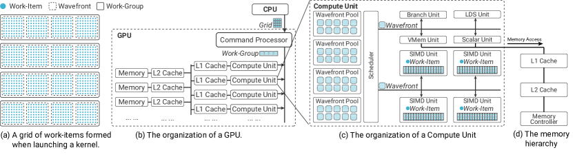
A program that runs on a GPU is called a kernel. As depicted in Figure 1(a), a kernel is composed of a large number of work-items that can be executed concurrently on a GPU. A work-item is similar to a CPU thread that runs a series of instructions (e.g., add, multiply) to process data. A certain number of work-items (typically 32 or 64, determined by the hardware) can be grouped into a wavefront. Wavefronts (typically 1–8) are further grouped into a work-group. Table 1 provides an overview of key concepts in GPU architecture that will be frequently described throughout this paper.
Software elements (e.g., kernels, work-groups, wavefronts, work-items) need to be mapped to hardware resources for execution. We illustrate how the kernel is executed on a GPU with Figure 1 (b) and (c). The CPU launches the whole kernel on a GPU for execution. On the GPU side, the Command Processor receives the kernel launch request from the CPU and divides the kernel into work-groups. After this, the Command Processor dispatches the work-groups to the Compute Units. Compute Units, similar to CPU cores, are responsible for calculating the program output. When work-groups are dispatched to a Compute Unit, the work-groups are broken down into wavefronts. Instructions that make up each wavefront wait to be scheduled by a central scheduler in each Compute Unit. The central scheduler dispatches instructions to the proper execution units, according to the type of each instruction. For a majority of the calculations, the instruction is sent to a SIMD unit (a digital circuit that can process instructions from multiple work-items at the same time).
| Concept | Description |
|---|---|
| Kernel | A snippet of a program that runs on a GPU. |
| Work-item | A GPU thread that executes instructions to process data. A work-item runs in parallel with other work-items. |
| Wavefront | A group 32 or 64 work-items that always execute the same instruction at the same time. |
| Work-group | A collection of 1–8 wavefronts. Wavefronts from the same work-group execute on the same Compute Unit. |
| Compute Unit | A GPU core that can run instructions |
| Component | A collection of closely-related digital circuits that perform well-defined functionalities. |
| Instruction | A few bytes (typically 4–8) that determine how the data needs to be processed. Examples are Add, Multiply, and Division instructions. |
| Cycle | The duration of time when digital circuits update their internal states. Digital circuits update states periodically. |
GPUs can process a large number of work-items concurrently. As a concrete example, we next present the organization of the AMD Radeon R9 Nano GPU (used in the case study and user evaluations). One GPU has 64 Compute Units; each Compute Unit has 4 SIMD units; and each SIMD unit can calculate instructions from 16 work-items in one cycle. Therefore, the whole GPU can calculate instructions at the same time. In addition, the GPU runs at a 1 GHz frequency (1 nanosecond per cycle), meaning that a GPU can execute 4 trillion instructions in 1 second in all the SIMD units in the R9 Nano GPU. Given the large number of instructions that a GPU runs, it is essential to support visualization of this massive amount of information, while still providing the capability of interactively viewing and zooming into the execution at a fine granularity (e.g., sub-nanosecond level).
In addition, Compute Units need to read data from the memory system (as shown in Figure 1(d)). After the data is copied from the CPU, the data is stored in the GPU’s main memory, which is managed by a set of memory controllers. Due to physics limitations, memory is not fast enough to feed the data required by the Compute Units. To increase memory throughput, GPU designers place faster, but smaller, storage close to the Compute Units. Caches are organized in tiers and are labeled as “Level 1” (L1) or “Level 2” (L2) caches, with the L1 caches being the smallest and fastest storage that are placed the closest to the Compute Unit. In many applications, the memory system implementation is limiting the performance of the whole GPU. Examining the memory system in the visualization tool is critical in understanding the overall GPU performance.
1.2 GPU Simulators
GPU simulators [gpgpusim, multi2sim, multi2sim_kepler, sun2019mgpusim] recreate the behavior of the GPU hardware and can run on a CPU without a GPU. GPU hardware designers can run GPU simulators and gather key performance metrics from execution traces generated by the simulator. A sample performance metric gathered from an execution trace would be the total execution time, which researchers can use to make an overall performance comparison. A GPU simulator can also dump simulation details (i.e., traces) to a file to record all the execution events that occur during a simulation. Since the trace is highly detailed, simulating a microsecond GPU execution can easily generate several GBs of trace data.
2 Related Work
Performance analysis tools have been developed both in industry and in academia to aid research on both CPUs and GPUs. In this section, we discuss the related performance analysis tools.
2.1 CPU Performance Visualizations
Many performance visualization tools facilitate debugging performance issues in CPU programs. They can be categorized in three groups: Icicle plot-based function execution time visualization typically uses icicle plots [kruskal1983icicle] or flame diagrams [gregg2016flame] to show the hierarchical relationship between function calls, as well as function execution time. Example tools include perf [PerfWiki77:online], gperftools [gperftoo65:online], callgrind [Valgrind35:online], Chrome Developer Tools [chrome], and Very Sleepy [VerySlee30:online]. Call graph-based visualization applies a network to show function call relationships and uses the node size and link width to visualize the execution time. Example visualizations are pprof [pprofREA88:online] and kcachegrind [KCachegr71:online]. Pipeline-based visualization tools use a multi-stage Gantt-chart [clark1922gantt] representation to show how hardware executes instructions. TraceVis [roberts2004tracevis] is one classic example pipeline-based visualization.
These visualization approaches are appropriate and sufficient for a single-threaded CPU execution and can help software engineers debug performance issues. However, they do not scale well for understanding individual hardware execution events happening on massively-parallel computing hardware. Daisen differentiates by focusing on visualizing hardware tasks (e.g., instruction execution, cache access) to explain GPU performance bottlenecks. GPU performance visualizations need to reveal the relationships between tasks that are executing at the same time, as well as allowing users to examine extremely low-level details from a tremendous amount of data.
2.2 GPU Performance Visualization
GPU vendors (e.g., AMD, NVIDIA) have created profilers for developers to examine the performance of GPU programs [radeon_gpu_profiler, profiler2014nvidia]. However, these tools are proprietary and users are forbidden to customize and to add new views. Also, since these tools are mainly designed for GPU software developers, they only capture high-level performance metrics and hardware execution information. GPU hardware designers need to save each nano-second in the repeated operations executed by GPUs to improve overall GPU performance, and hence, need to access sub-nanosecond-level execution details. Due to the lack of extremely detailed GPU execution information, industry profilers cannot fulfill the requirements of GPU hardware designers.
There have been tools specifically designed for visualizing GPU execution. AerialVision [aerialvision] provides a time-lapse view to allow tracking several performance metrics over time, as well as a source code view that displayed statistics associated with individual lines of code to help identify the source of bottlenecks. M2S-Visual [M2S-Visual] is an interactive visualization tool that is specifically customized to visualize execution traces generated by Multi2Sim [multi2sim]. These visualization tools can hardly be adapted to support examining data generated from other simulations since they did not provide a generic data abstraction model. Moreover, both AerialVision and M2S-Visual can only visualize predefined aspects of GPU execution, such as instruction pipeline stalls, cache utilization, and network congestion. These tools require developing new views for each new simulator features, adding extra burden to visualization tool developers. Therefore, there is an essential need to build a universal trace format that represents behaviors across the various hardware components implemented in different simulators. Doing so will help promote generality in terms of data collection and benefit future design of the GPU architecture. Collectively, examining GPU performance requires a significant effort in parsing the traces generated by GPU simulators. Visualizing a large volume of traces mitigates the user’s burden and helps users understand application behaviors more efficiently [aerialvision]. However, visualization research on GPU executions is still in its early stages. Our work seeks to address this research gap and contribute to GPU performance visualizations.
3 Task Analysis and Abstraction
We conducted a survey study with 37 computer hardware designers who have had past experience with parallel computing system performance analysis. We created the survey using Google Forms and distributed via social media (e.g., Twitter, Slack) in a convenient format. We open coded [thomas2006general] the comments and free-text answers to generate themes regarding the workflow of identifying performance and bottleneck issues. We also conducted informal interviews with five GPU hardware designers to further refine the design requirements and characterize practices and common workflows when using simulators.111This study was approved by the Institutional Review Board at our institution.
Based on the survey results and interviews, we performed a task analysis to characterize domain problems, followed by task abstraction that aims to recast user goals from domain-specific languages to a generalized terminology for better understanding and readability [munzner2014visualization]. We chose a Hierarchical Task Abstraction [zhang2019idmvis] since performance analysis in computer architecture is a dynamic process that typically involves multiple hierarchical abstractions. A Hierarchical Task Abstraction is useful to capture task hierarchies, task sequences, and task contexts [zhang2019idmvis].
3.1 Task Analysis
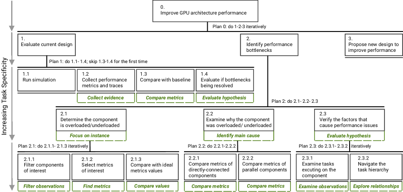
We created a task analysis for GPU hardware design, shown in Figure 2. The overall goal of GPU hardware designers is to improve GPU performance by proposing new GPU hardware designs (Task 0). The first step is to evaluate the performance of the current design (Task 1). In the first iteration of this step, designers evaluate the performance of the baseline design by running a simulation (Task 1.1) and collect performance metrics and GPU execution traces (Task 1.2).
After collecting the execution traces, GPU hardware designers need to identify the performance bottlenecks (Task 2). As the first sub-step, designers examine the load of each component (Task 2.1). For example, an experienced designer can check the “Number of Executing Instructions” metric of the SIMD units to understand if the workload is compute-intensive. If the SIMD units are underloaded, the running application is deemed not compute-intensive, eliminating the possibility of identifying SIMD units’ computing capability as the performance bottleneck. To complete this process, designers need to filter the component (Task 2.1.1) and select the metrics to examine (Task 2.1.2). After this, designers can assess the load of each component by comparing the achieved values with the anticipated values (Task 2.1.3). For an example of such expected values, a SIMD unit can process one instruction at a time. Therefore, the expected value is 1. If the achieved “Number of Executing Instructions” is significantly smaller than 1 for the most of the execution, the SIMD units are underloaded.
After identifying the load of the components, designers need to find the main reason for the underloading or overloading of components (Task 2.2). This process typically includes a comparison between directly-connected components (Task 2.2.1) to determine which component is issuing insufficient requests or issuing too many requests. Designers also compare components that are at the same level in the hierarchy (Task 2.2.2) to see if the loads are evenly distributed. For example, a GPU is equipped with multiple memory controllers to work in parallel to serve more memory requests. An experienced designer can check the load of the memory controllers to see if one controller is receiving more requests than the others, as workload imbalance can reduce the speed of serving memory requests, limiting overall performance. By comparing and reasoning about the relative load of related components, a designer can pinpoint which component is causing a performance bottleneck.
To verify the hypothetical performance bottleneck, GPU hardware designers typically examine what happens in a short period of time (Task 2.3). They typically first check the tasks executing in a particular hardware component (Task 2.3.1). For example, they check all the instructions executing in a Compute Unit to see which instruction is preventing the Compute Unit from making further progress. They also check the task hierarchy (Task 2.3.2). E.g., a designer needing to check which instruction generates long-latency memory accesses.
After identifying the bottleneck of the current platform, the GPU hardware designers need to propose new designs that can mitigate the performance bottlenecks (Task 3). This step mainly relies on problem-solving skills and prior experience, so is out of the scope of our visualization work. After developing a new design, designers need to repeat Task 1. This time, however, they need to compare the result with the baseline design (Task 1.3) and examine whether the bottleneck is resolved as expected (Task 1.4). If the performance of the new design cannot reach the performance goal, designers will look for a new performance bottleneck in the new design (Task 2). Designers typically need to repeat Tasks 1–3 many times until they find a solution that satisfies the design requirements.
3.2 Task Abstraction
Based on the task analysis, we performed a task abstraction that aims to recast tasks from domain-specific languages to a generalized visualization terminology to achieve better understanding and readability [munzner2014visualization]. We generate task abstractions guided by Amar et al.’s [amar2005low] low-level components of visual analytics and Lam et al.’s framework [lam2018bridging] that focuses on connecting analysis goals and steps in design studies. The abstractions, labeled green in Figure 2, are integrated with the Hierarchical Task Abstraction guided by Zhang et al.’s work [zhang2019idmvis].
4 Design Requirements
We identified a set of design requirements of GPU execution trace visualization based on our survey results and informal interviews with GPU hardware designers, as well as data and task abstractions discussed in the previous section. We divide the design requirements into functional requirements and non-functional requirements.
Functional Requirements:
We identified four functional requirements (FRs) [RogersYvonne2011IDbh] for an appropriate visualization:
FR-1: Support visualizing a large number of concurrently-executing tasks. Hardware elements typically achieve a particularly high degree of parallelism. Thousands of components may execute different tasks at the same time. Each component may also execute a large number of tasks in parallel.
FR-2: Create a mapping between software concepts and hardware concepts. It is essential to examine how the software elements (e.g., memory access) are executed on hardware components (e.g., caches). If designers question why a software element is not executed early enough, they need to investigate why the hardware elements are busy.
FR-3: Allow for efficient browsing through the execution and zooming down to focus on a short duration gradually.
Simulation traces record execution that last milliseconds to seconds. Meanwhile, researchers need to identify hardware behavior at a sub-nanosecond level.
FR-4: Be generic enough to reveal the execution details of many different hardware components.
Researchers may need to inspect a wide range of components associated with hardware execution. Designing a visualization view for each individual aspect is not practical.
Non-functional Requirements:
In addition to functional requirements that traditional visualization tools specify, we also identified two non-functional requirements (NFRs) [RogersYvonne2011IDbh] that are critical in the design and implementation of a visualization tool:
NFR-1: Social environment — Support bookmarking and sharing for better collaboration. Our survey respondents indicated that they need to bookmark and organize the discoveries and continue browsing from an earlier scene. They also need to discuss specific performance issues with other collaborators. Therefore, allowing users to share specific states of the visualization would help them communicate references of interest effectively.
NFR-2: Technical environment—Ensure efficient performance considering the tremendous mountain of data available in traces generated from GPU simulations. Scalability issues are one of the major constraints of trace-based performance [wolf2006large]. Therefore, it is critical to ensure smooth and efficient interactive visualization.
5 Data Abstraction
| Field | Format | Description | Example |
|---|---|---|---|
| ID | Text | The unique identifier of a task, which was randomly generated to guarantee uniqueness | 5C9dX8 |
| Parent ID | Text | The ID of the parent task | 7F3sY2 |
| Category | Text | The category of the task belongs to | Instruction |
| Action | Text | The job of the task indicating what the task is doing | Read Memory |
| Location | Text | The hardware component that carries out the task | CPU1.Core1 |
| Start/ End | Time | The time that a hardware component starts to process/ completes processing the task | 0.00014566s |
| Details | JSON | Any other information | {"inst":"add"} |
We first map data into a unified format. The goal is to build a cohesive and comprehensive data collection framework to help users make sense of the volumes of data and identify performance problems.
We define every entity of collected data as a task (see Table 2). Each task is assigned a unique ID that identifies unique execution during a simulation. A task is also assigned information describing which category it belongs and the job of the task, captured in the “Category” (e.g., “Request Out”, “Request In”, “Instruction”) and “Action” (e.g., “Read Memory”, “Execute ADD Instruction”) fields, respectively.
The most common “Category” of the tasks are “Request Out” and “Request In”. These tasks capture the communication between most of the components. When a component (Component A) initiates a task that needs to be fulfilled by another component (Component B), Component A sends a request to component B. Later, when Component B completes the request, Component B replies to Component A with a response message. As a typical example in GPU hardware architecture, a Compute Unit may send a read request to a cache. Later, when the requested data is available, the data cache sends a data-ready response back to the Compute Unit. We summarize this request and response process as two tasks. The first task’s duration, with type “Request Out”, starts when Component A creates the requests until Component A receives the response. The “Request In” task is a sub-task of the “Request Out” task. It starts when Component B receives the request and finishes until Component B sends out the response.
The simple “Request In” and “Request Out” tasks carry rich information about the execution. For example, hardware designers usually have an expectation of the number of requests that a component can serve. By calculating the number of “Request Out” completion per second, we can verify whether the component meets the efficiency requirement. In addition, the time between a “Request In” initiation and the corresponding “Request Out” initiation represents that the request is waiting in a queue to be processed. We can calculate the number of requests that are being buffered in the queue at a component at any specific time point. A prolonged “high buffer level” duration suggests that the component may be a performance bottleneck, and increasing its processing speed may improve overall system performance.
The name of the component that carries out the task is recorded in the “Location” field. We require a task to only have one location. A task that involves multiple components should be treated as multiple tasks. Each task has a Start time and an End time. Users can also include extra information in the “Details” field. We do not use the detailed information in the visualization directly to maximize the generality of the visualization tool. But users can see the details on the side of the visualization views when they hover their mouse pointer over a task.
Tasks are organized hierarchically using a tree structure. Each task has a “Parent ID” field, keeping track of the ID of its parent task. Locating all the subtasks of a particular task requires a SQL query (e.g., SELECT * FROM tasks WHERE parent_id="5C9dX8";). The only task that does not have a Parent ID is the root task, which represents the entire GPU program execution.
6 Visualization Tool
Next, we introduce Daisen’s visualization tool, an open-source, web-based, interactive visualization tool that aims to help GPU hardware designers evaluate the performance of GPU designs. We highlight its capability of fulfilling the functional and non-functional requirements with three unique perspectives, including the Overview Panel, the component view, and the Task View.
6.1 Overview Panel
A simulation of a few milliseconds of hardware execution can generate millions of tasks and GBs of data. A user can be overwhelmed by the large amount of detailed information and may ignore important trends. The Overview Panel provides the ability to see the big picture of the execution under evaluation and helps users identify the major trends of how the metrics change over time and locate interesting time intervals that require closer investigation. The design of the Overview Panel partially satisfies FR-3, as well as supports Tasks 2.1 and 2.2.
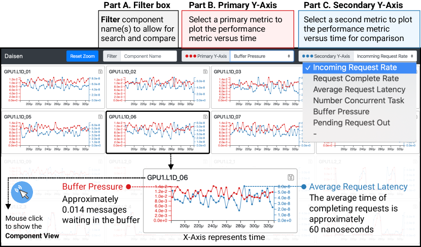
The Overview Panel, as shown in Figure 3, displays a series of small multiples, with one diagram representing a component in the simulation. Since there can be hundreds to thousands of components in a single simulation, we separate the components into multiple pages. Users can browse the components by visiting each page. Moreover, we provide a filter box (see Figure 3 Part A) to enable users to filter the components of interest (as required by Task 2.1.1).
We display all the component diagrams as time-series visualizations, with the x-axis indicating the simulation time. Users can select key metrics of interest to explore using a drop-down menu. They can also choose the metrics for both the primary y-axis (see Figure 3 Part B) and the secondary y-axis (see Figure 3 Part C). Users typically need to see more than one metric as they need to find the relationship between multiple metrics to determine if they are positively correlated, negatively correlated, or uncorrelated.
We currently provide 6 general metrics for the y-axes, including the request arrival rate, request completion rate, request completion latency, number of concurrent tasks, buffer pressure, and number of pending outgoing requests. The choices of the y-axes were based on the survey responses and feedback with domain experts. We avoid component-specific metrics (e.g., cache hit rate) to keep the visualization framework general. Generally, users can still infer component-specific metrics from these metrics.
Users need the ability to compare the performance metrics of multiple components in order to identify performance issues. To support Task 2.2, users are able to filter components to compare metrics (e.g., Figure 3). Since the filter box supports regular expressions, a user can easily use partial names (e.g., L2), or use a regular expression (e.g., "(CU|L1|L2)"), to create any combination of components. Moreover, when a user zooms or drags in a diagram, the time axes of all the diagrams will be updated to show the curves of the same time period. This creates an alignment effect and can help users compare the behavior of different components [zhang2019evaluating].
Once the user arrives at an initial guess for the cause of the performance bottleneck, they may need more detailed information to verify the performance bottleneck, as in Task 2.3. The user can first zoom into a short, specific time period in the Overview Panel and click the component name to see the tasks executing during that period in the Component View.
6.2 Component View
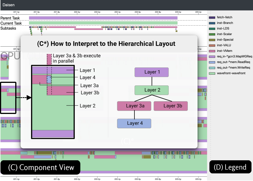
The Component View, as shown in Daisen: A Framework for Visualizing Detailed GPU Execution(C), shows all the tasks executed at a certain component. The Component View aims to help users understand how hardware resources are utilized. The current component name (using transparent text) on the top-left corner of the Component View helps remind users which component they are currently viewing.
Each rectangle represents a task. The left and right positions indicate the start and end time of a task. The width of the rectangle represents the task duration. This Gantt-like chart design is consistent with existing trace or task visualization tools [roberts2004tracevis, chrome]. Using a style that is familiar to the user group can smooth the learning curve and reduce mental burden [RogersYvonne2011IDbh].
We choose to present the task visually in a hierarchical way to avoid cluttering and allow users to better understand the relationship between the tasks (as depicted in Figure 4). In the Component View, root tasks (a task that has no parent task or its parent tasks have a different location) are directly displayed on the canvas. Each task uses its internal space to show its subtasks. Also, tasks at the same level are assigned the same height to be consistent.
Existing task visualization tools [roberts2004tracevis] usually assign a row for each task. However, this simple row-assignment scheme is not practical for GPU execution visualizations because GPU execution is massively parallel. A component can execute a large number of tasks at the same time. Assigning a row to each task requires too many rows, making each row too narrow. Therefore, in the Component View, we use an up-floating layout algorithm to determine where to place the task bar. We assign the row number for each task in the order of the task start time. Each task is assigned with the smallest row number (top-most row), as long as it does not overlap with any task that is already assigned with a row number. In this way, we can use the minimum number of rows and show the maximum height possible for each task, while guaranteeing that tasks do not overlap with each other. Users can rely on the number of rectangles stacked at the same x-position, to know how many tasks are executing in parallel at a certain component at a particular time, indicating how busy the component is.
We use color-coding to differentiate tasks based on their “Category” and “Action”. One challenge to manage is that since the tool is generic to all types of hardware components, we cannot exhaustively list all the possible “Category” and “Action” values apriori. We need to dynamically color the tasks. To solve this problem, we use the Cubehelix [cubehelix] coloring scheme, as Cubehelix creates contrast in both the hue and the lightness, ensuring readability and accessibility for colorblind users.
We reserve the right sidebar of the interface to provide information that may help users understand the diagrams. By default, color-coded information is displayed as a legend. The legend also allows users to find tasks of a particular type easily. When a user hovers the mouse pointer on a legend element, the tasks in the Component View, as well as the tasks in the Task View, will be highlighted with bolder outlines, while the rest is grayed out. The right sidebar can also provide additional information for each individual task. When the user hovers their mouse pointer on a particular task in the Component View, the detailed information (listed in Table 2) will be shown above the legend.
6.3 Task View
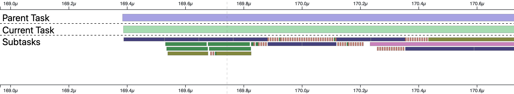
The Component View demonstrates how the hardware is utilized. It aligns with a typical hardware performance analysis scenario. However, users also need to analyze the performance using a software performance analysis approach. They usually need to answer the question about why a particular task takes such a long time or which subtask takes the longest portion of the total time. Although the Component View displays tasks in a hierarchical way, it cannot show subtasks that are not executed in the current task, and hence, does not allow the user to move up or down the entire task hierarchy, as required in Task 2.3.2. To solve these problems, we supplement the Component View with a Task View. A user can click on a task in the Component View to enable the Task View. The selected task becomes the “current task”.
As shown in Figure 5, the Task View shows three groups of tasks. The second row of the task bar shows the “current task”. Above the current task is its parent task. We show the parent task for two purposes. First, users can understand the relative timing relationship between the current task and the parent task, answering the question of whether the current task is a major step required to complete the parent task. Second, users can click on the parent task to navigate towards the root of the task hierarchy, getting a larger picture of program execution and partially fulfilling FR-3.
All the subtasks of the current task are displayed below the current task. We reuse the “up-floating” algorithm to maintain consistency with the Component View and to save space. Showing the subtasks allows users to discover how the time is spent to complete the current task. Users can click on one of the subtasks to set that task as the “current task” or to drill down for a more detailed view. Combined with the parent task, the subtasks support navigation up and down through the entire task tree, fulfilling FR-3.
The Task View is stacked on top of the Component View. Their time axes are always aligned. Dragging or zooming one view always refreshes both views. Aligning the time axes helps the user to easily match the tasks in the Task View (software concept) and the Component View (hardware concept). When a user hovers over a task in either the Task View or the Component View, the task is highlighted on both sides to help users establish the connection between these two views. A typical use case is that a user may need to know why a task is not executed immediately after the previous task is completed. To answer this question, the user can check what the component was doing earlier. These two tasks are competing for hardware resources. As we align the Task View and the Component View, it should be straightforward to find the tasks that the component is executing at the time. The alignment of the Task View and the Component View can fulfill FR-2.
Since all three views do not rely on any component-specific data, they are generic and can be applied to visualize any digital circuit, fulfilling FR-4. In addition, as the visualization tool is decoupled from the data collection tool and the simulator implementation, it can be used to view any hardware execution data that adopts Daisen’s data abstraction.
6.4 Implementation
Daisen’s data collection library has been implemented for a generic GPU simulation framework [sun2019mgpusim]. The same mechanism can be adopted for most computer architecture simulators or can capture live hardware executions. We store the collected data in a MySQL database.
After the simulation completes, users need to start the backend server. We implement the backend server with the Go programming language. The server application reads the data from the database, processes the data, and sends the data to the frontend upon request. The frontend is implemented using TypeScript and the D3.js [bostock2016d3] visualization library. The server and the client can be executed on the same computer or different computers. This server-client model does not require users to install any library or software except a web browser. The server-client model also enables multiple users to check the results at the same time.
We use the browser URL to encode the current scene to achieve 3 goals. (1) Users can use the browser’s bookmark functionality to bookmark interesting scenes for future reference [roberts2004tracevis]. (2) At any time, a user can copy the URL from the browser’s address bar and share the URL with others. The URL can be shared with others to see the same scene and start exploring the simulation results from the scene encoded by the URL. (3) We do not need to implement the navigation buttons (i.e., the backward and forward buttons). Users can easily use the browser’s forward and backward control, which is both intuitive and space-saving. They can even use the browser’s history to revert back to any scene visited before. By combining a server-client model and a URL encoded view, we fulfill the requirement of NRF-1.
Performance and smoothness can be a major challenge of implementing a web-based data-visualization tool. Therefore, we take three steps to guarantee the performance and smoothness to fulfill NRF-2. (1) We properly create indices for the database columns, reducing database access latency. (2) We use asynchronous refresh. When a user drags or zooms in the interface, we manipulate the elements on the screen, providing latency-free feedback to users. After the user stops dragging or zooming, the frontend requests data from the backend, updating the element on the screen to guarantee the correctness of the content. (3) We ignore the elements that do not provide useful information to users. For example, if a bar in the Component View is too small, we do not show it on the screen, limiting the total number of rendered elements.
Seeing the requirement that hardware designers need to report the performance analysis findings in technical writings, the visualization tool allows saving diagrams as Scalable Vector Graphics (SVG) files, simplifying the process of exporting visualization results for technical reports or papers.
7 Case Study
We use a case study to demonstrate how Daisen can help improve the performance of a GPU architecture design. We simulated the execution of the PageRank benchmark from the Hetero-Mark benchmark suite [sun2016hetero] running on an AMD R9 Nano GPU [r9nano]. PageRank [pagerank] is widely used by search engines to determine the importance of websites. It is a commonly used data-mining application that benefits from the GPU’s massive-parallel computing capability [pagerank-gpu-1, pagerank-gpu-2]. We ran the PageRank algorithm over a dataset with approximately 66K websites and 420K hyperlinks. We only ran one iteration of the algorithm as the GPU demonstrates similar behavior during each iteration. We used the AMD R9 Nano GPU in this example as it is the default GPU configuration provided by MGPUSim [sun2019mgpusim]. The same analysis approach is applicable to most GPUs. The rest of the case study follows the user process described in Figure 2.
7.1 Bottleneck Analysis
We first ran the PageRank benchmark [pagerank] on MGPUSim. MGPUSim simulated the execution of the program on the R9 Nano and reported that PageRank could run in . The simulation generated a trace with tasks. The traces consumed of disk space.
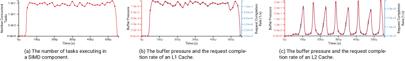
The first task was to check which component was underloaded or overloaded to examine if the workload was compute-intensive or memory-intensive. To check compute intensity, we first checked the utilization of the SIMD unit (digital circuits that run the calculations) by filtering the SIMD unit by entering “SIMD” in the filter box and choosing “Number of Tasks” as the primary y-axis in the Overview Panel. According to Figure 6(a), the SIMD utilization was low, suggesting it was not a compute-intensive workload. We then checked the “Buffer Pressure” and the “Request Completion Rate” for the L1 and L2 caches. From Figure 6(b) and (c), we were able to conclude that both the buffers of the L1 and L2 caches were empty for most of the time and the Buffer Pressure value was constantly smaller than 1. We can conclude that this work was not memory intensive either.
Since the L1 cache was not given enough tasks (as suggested by the low buffer pressure), we further examined the Component View by clicking on the L1 cache widget title. In the Component View, we identified long gaps between tasks, indicating the L1 cache is idle for most of the time. After this, we attempted to make sense of why the L1-Cache tasks did not start earlier. To reason about the process, we selected the second task to enable the Task View. We kept using the “parent task” bar in the Task View to trace back to the root of the tree.
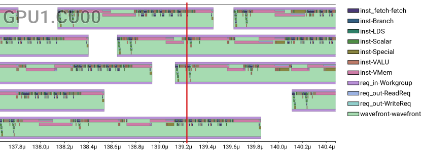
As we traced back to the Compute Unit, we could check the memory instructions that triggered the L1 cache access. We could identify that the reason why the L1 did not have enough tasks was because the memory instructions were executed infrequently. Ideally, each Compute Unit can run 40 wavefronts (as shown in Figure 7), so that there should be a large probability that at least one wavefront issues a memory instruction. However, in Figure 7, we can see that only 3-5 wavefronts were executing in parallel. These wavefronts might be all executing compute instructions or waiting for existing memory accesses to complete, so they cannot generate new memory accesses. After making sense of the performance issue, we concluded that the root cause might lie in the Compute Unit that was not executing enough wavefronts. The global performance bottleneck was that the Command Processor was not running fast enough to dispatch work-groups.
7.2 Solution Evaluation
Since we know that the Command Processor dispatching process was the global bottleneck, we aimed to improve the dispatching algorithm and the dispatching speed from 1 work-group per cycle to 2 work-groups per cycle (similar design decisions were made in the most recent AMD Navi GPUs [navi]). We implemented a new algorithm in the simulator and re-ran the experiment. We validated our design as the new simulation output matches the desired algorithm output. According to the simulator, this simple improvement reduced the GPU execution time from to , speeding up the execution by .
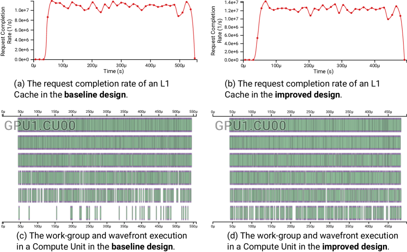
Next, we analyzed whether the improved design can mitigate the performance bottleneck. We first compared the request completion rate at an L1 cache. According to Figure 8 (a) and (b), we can see that the new design increases the request completion rate from 11 million requests per second to 12 million requests per second, improving the effective memory system throughput. Moreover, as we compared the work-group and wavefront execution in Figure 8 (c) and (d), we were able to see that the compute unit had been executing more work-groups at the same time. The number of work-group tasks on the 6th row was significantly increased, indicating a higher level of execution parallelism. Overall, our simple design change relieved the performance bottleneck and successfully improved the overall GPU performance. Meanwhile, we could also see that there remains a significant space to further improve device utilization and to improve performance.
8 Evaluation
To further evaluate Daisen, we conducted user studies with 10 participants who had prior experiences in GPU hardware design. The average time they have been working in performance analysis was 4.6 years (). The highest degree of education among participants was split equally between master’s degrees () and doctorates (), with one bachelor’s degree and one associate’s degree.
8.1 Methodology
We conducted our evaluation study remotely using online communication tools (e.g., Slack, Zoom). We asked participants to share their screens with us to allow us to observe how they interacted with the visualization. The evaluation study includes five parts. First, participants were provided with a walk-through tutorial to help onboard them. Second, they were asked to explore the tool on their own using the “think-aloud” method [lewis1982using] that encourages verbalizing their thoughts as they move through the visualization. In this process, they were asked to explore a dataset different from the onboarding tutorial. Third, they were asked to identify a performance bottleneck from the dataset they examined. Fourth, we conducted follow-up semi-structured interviews about their experience interacting with the tool, such as what was easy or difficult to understand, what they liked or disliked about the tool, and what changes they would like to make to further help them identify performance issues. Lastly, we asked each participant to fill out a post-study survey regarding how well Daisen facilitates performance analysis. The whole session lasted approximately 90 minutes for each participant.
8.2 Findings
During the evaluation study, 9 out of 10 participants were able to identify bottlenecks successfully with the help of Daisen. Our participants also gave positive feedback on Daisen, especially how Daisen can be used to help them identify and make sense of performance issues.
Value of visualizing GPU traces in Daisen: Our participants appreciated the visualization of GPU simulations and some expressed their excitement of using Daisen to examine GPU performance issues. Our participants described how they typically visualize execution information. Half of them indicated that they first added “print functions” in the GPU simulator to get more performance information, exported to a CSV file and then visualizing the trace data separately (in Python) to explore and identify performance issues. For example, P03 said “My debugging is using prints to get any of these numbers. But is also cumbersome to either have another script to process those files and then read them.” P03 further appreciated Daisen’s capability to help with GPU architecture design. P03 said, “Daisen gives a pretty good picture of this benchmark is suffering because of certain factors. Then I can take a design step to improve something.” P07 also liked how Daisen supports visualizing GPU traces by comparing with other trace visualization tools, such as VTune [reinders2005vtune] and nvprof [nvprof]. P07 mentioned that “nvprof also gives you some kind of views but can only show which kernels are running (from a high-level and coarse-grained perspective). However, Daisen enables users to understand which portion and phases of the application are getting low [performance] and have problems.”
In addition, Daisen’s generic design supports user needs well and its lack of support for component-specific metrics did not seem to impact usability. For example, P07 said, “Maybe I am more used to looking at hit rate and miss rate (component-specific statistics in GPU simulation). But I think [Daisen] gets the timing statistics pretty accurately (highly detailed). I think they (component-agnostic metrics and component-specific metrics) are pretty much the same. You can get an idea of the hit rate and the miss rate by just looking at the metrics here.”
Overview allows for quickly identifying hot spots: The Overview Panel enables users to explore high-level simulation behaviors and identify performance issues. Participants frequently interacted with the filtering function, zooming in and out to search for potential hot spots that took longer in execution. P05 specifically valued being able to browse behaviors of various components, as “it gives the users the ability to verify their hypothesis on different applications and see which resources cause the constraint in the system.”
Task view enables navigate between components: Our participants used the Task View mainly to navigate across components, as well as explore execution relationships between the Task View and the Component View. P04 and P08 particularly liked the Task View’s ability to navigate between components. P08 said “It is really really nice to have this type of navigation between tasks and subtasks.”
Component view helps examine low-level simulation behaviors: Our participants mainly used the Component View to get a more in-depth understanding of the performance of a particular component, especially when they saw conflicting things happening in an overview. For example, P03 recalled a situation where he needed a detailed view. He explained that when he tried to understand what instructions the workload was executing, he needed more evidence to support his hypothesis on how to improve the design with the help of the Component View. Similarly, P01 specifically mentioned how well Daisen helped him understand simulation behavior as compared with some profilers he had used before. He commented that existing profiling tools failed to provide sufficient detail for making sense of performance issues.
Though all the participants foresee themselves using Daisen to facilitate their research in GPU hardware design and computer architecture research, they also suggested a few things that can be improved to better help them examine GPU performance issues. These features include: (1) support for visualizing GPU performance while the simulation is running, (2) educational support and tutoring, such as automatic screen recording and more user guidance, and (3) integration of summary statistics into Daisen to enable users with various levels of visualization literacy to understand the performance (e.g., statistically summarizing 70% of the instructions being executed).
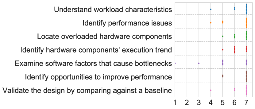
Post-study Survey Results: Overall, as shown in Figure 9, participants found that using Daisen helped them understand key characteristics of workloads (, ), identify performance issues (, ), locate overloaded hardware components (, ), explore trends in executions (, ), examine software-related factors that cause the performance bottlenecks (, ), identify opportunities to improve performance (, ) , and validate the new design by comparing with a baseline (, ).
9 Discussion
Participant feedback about Daisen was very positive overall. In this section, we reflect on the design and evaluation of Daisen. One challenge we encountered when designing a visualization research study is that we have to make tradeoffs between generalization and specialization. On the one hand, we can pursue generalizability that aims to benefit a wider range of audiences [thudt2017expanding]. On the other, design studies have focused on seeking solutions for a particular problem domain [munzner2008process]. Keeping these criteria in mind, Daisen’s design prioritizes providing a generalized data abstraction and visualization framework that can be both applicable to other domains and can support examining GPU simulations effectively.
To maintain generalizability, Daisen provides six data-collection API functions (two for tasks, four for requests) to support data collection. Users can use these APIs to annotate (i.e., inserting the function call at critical execution point) hardware simulators or applications to collect data for visualization. Within the broader computer systems research arena, Daisen’s approach can be used to support the design of a wide range of hardware and software systems, whether the focus is on task dispatching or job scheduling [li2017optimal, meng2019dedas]. The data abstraction model of Daisen is general enough to capture the semantics of task dispatching and job scheduling behaviors. The visualization is also designed to be generally applicable to support the investigation of resource utilization during task execution. We encourage GPU researchers to apply Daisen’s data-collection library to their own simulators so that they can use Daisen’s visualization tool to help examine performance issues and improve GPU performance.
Our effort to maintain a general framework also created some challenges for our participants. For example, since we do not know all the possible components used in a simulation (i.e., the visualization tool may need to visualize very different hardware), we cannot sort the components in the Overview Panel in the most straightforward way. Also, since we simplified the data abstraction and data collection interface, Daisen did not support collecting component-specific data such as the cache hit rates. During our evaluation study, although most participants indicated that they were able to infer the component-specific metrics from the component-independent metrics, some (P03, P07) also wanted to see “traditional” component-specific metrics to help them understand the execution. Therefore, more work is needed to examine the best trade-off between generalization and specialization.
We also noticed that more experienced GPU designers more quickly grasped key concepts using the generic terms provided in Daisen. This shortcoming raises a question for future research: how to design a visualization environment for users with different levels of expertise and help overcome the steep learning curve. Many approaches have been explored to help users comprehend how visualization works, such as step-by-step wizards, forums, and animated video tutorials [fernquist2011sketch, grossman2010toolclips, matejka2011ambient, pongnumkul2011pause]. In addition to these strategies, our evaluation results suggest that allowing the user to customize metrics (e.g., instruction per cycle, cache hit rate) may be a solution to address different degrees of user expertise.
Limitations: The aim of the survey was to examine the workflow of carrying out a performance analysis and guide us to help characterize domain tasks and processes. However, we are aware that the survey results may have potential bias since we used convenience sampling for recruitment (e.g., under-representation of subpopulations in the sample). Therefore, we avoid making absolute claims when analyzing and reporting our survey results. Care should be taken when making inferences based on our convenience sample.
10 Conclusion
In this paper, we describe Daisen, a visualization framework designed for visualizing execution traces generated by GPU hardware simulators. We defined a versatile data abstraction that can capture the behavior of a wide range of hardware components. We also developed a web-based visualization tool that reveals rich hardware execution information. We incorporated three views to show different aspects of the execution, including the Overview Panel, the Component View, and the Task View. We used a case study to show that the tool can identify performance bottlenecks of GPU hardware executing an application. Our interview with domain experts produced positive feedback, suggesting that Daisen can be a useful tool in their future hardware development toolbox.