How Are Learned Perception-Based Controllers Impacted by
the Limits of Robust Control?

Abstract

The difficulty of optimal control problems has classically been characterized in terms of system properties such as minimum eigenvalues of controllability / observability gramians. We revisit these characterizations in the context of the increasing popularity of data-driven techniques like reinforcement learning (RL), and in control settings where input observations are high-dimensional images and transition dynamics are unknown. Specifically, we ask: to what extent are quantifiable control and perceptual difficulty metrics of a task predictive of the performance and sample complexity of data-driven controllers? We modulate two different types of partial observability in a cartpole “stick-balancing” problem – (i) the height of one visible fixation point on the cartpole, which can be used to tune fundamental limits of performance achievable by any controller, and by (ii) the level of perception noise in the fixation point position inferred from depth or RGB images of the cartpole. In these settings, we empirically study two popular families of controllers: RL and system identification-based $H_{\infty}$ control, using visually estimated system state. Our results show that the fundamental limits of robust control have corresponding implications for the sample-efficiency and performance of learned perception-based controllers. Visit our project website https://jxu.ai/rl-vs-control-web for more information.

1 Introduction

Data-driven techniques for robotic control such as deep reinforcement learning have recently become increasingly popular, especially for settings where input observations are high-dimensional, such as images, and state transition dynamics are not known in advance. These techniques have shown great promise for controlling a variety of robots ranging from manipulators (OpenAI2018-qx) to legged robots (Lee2020-xx), drones (Molchanov2019-gz), and autonomous cars (kendall2019learning). However, these techniques have largely been studied and developed within the confines of stylized, often simulated settings, where performance metrics are naturally divorced from important real-world concerns such as safety and robustness. In the light of recent catastrophic failures of learning-based control systems such as fatal autonomous car collisions (wp_av-fatality), we argue that it is imperative to study and characterize the limitations of these approaches in challenging settings that present realistic difficulties for observation and control. In particular, how do such difficulties affect the performance and sample complexity of learned controllers?

Classical robust control theory provides a rich set of tools characterizing fundamental limits on achievable performance in terms of system properties such as open-loop unstable poles and zeros. However, analogous theoretical results in the learning-based control literature are not nearly as well developed, especially in the context of controllers that involve high-capacity functional approximators such as deep reinforcement learning from pixels. Rather than seeking theoretical limits, we try a different tack, empirically studying various families of learned controllers in a setting where control and observation difficulty can be carefully tuned.

Our empirical study focuses on the visuomotor control task of stabilizing a cartpole in the upright position using only the visual observations from a camera with a head-on view. All visuomotor controllers must implicitly or explicitly solve two important and closely intertwined problems. The first is visual perception, i.e., how to map raw high-dimensional visual observations $o$ to their task-relevant latent causes, denoted as the state representation $x$? The second is the task of synthesizing optimal action policies $\pi(u|x)$ conditioned on those state estimates.

In real-world settings, perception is often an underconstrained problem. For example, an autonomous car with on-board cameras cannot see around the corner of a street on a left turn, or a pedestrian occluded behind a parked vehicle, or a pedestrian with dark clothes on a poorly lit street. In all such instances, the observations $o$ are a non-invertible function of the relevant state $x$, and the estimated states $\hat{x}$ output from perception cannot match the state $x$ perfectly, even with the most optimal perception system. This imperfect perception problem may be represented formally as a partially observable Markov decision process (POMDP). The successes of reinforcement learning in the last few years have been largely demonstrated on fully observed tasks, and general methods for tackling POMDPs remain elusive. Even when they are evaluated on real-world robotic systems, robots and environments are typically instrumented to ensure near-complete observability of all relevant state information, which is impractical for in-the-wild applications like autonomous driving.

Our visual cartpole balancing task permits the modulation of two realistic sources of partial observability within the context of a well-studied classical control problem. First, a set fraction of the cartpole’s length is constantly occluded from the camera. As we will explain, this type of information loss has been shown to induce fundamental limits on the performance of any controller for this system. Second, the sensing abilities of the camera itself may also limit perception. For example, to estimate the distance from the camera of an object in the scene such as the cartpole, a perception system with access to RGB camera observations would be harder to train, and it would produce more noisy estimates than one receiving inputs from a stereo depth camera.

We study the impact of tuning these sources of perception noise on the performance of two families of learned controllers: system identification-based $H_{\infty}$ control and reinforcement learning, both using visually estimated system state. Our careful empirical studies clearly show that increasing occlusion and deteriorating sensing quality affect both families of controllers in ways that align well with theoretically predicted limits for classical robust controllers. In particular, sample complexity increases and final task performance decreases, and the effect of sensing noise is exacerbated as more of the cartpole is occluded from view.

1.1 Related Work

Fundamental limits of learning-enabled control.

Much of the research in the learning for control community has focused on characterizing achievable upper bounds on the performance of learning based control strategies. While such upper bounds are common in the literature, lower bounds are few and far between. For model-free RL methods as applied to the Linear Quadratic Regulator, such lower-bounds can be found in (tu2018gap), where the authors derive asymptotic lower bounds on the number of samples needed by both the least-squares-temporal-differencing estimator for policy evaluation, and policy gradient methods for policy improvement. In (simchowitz2018learning; simchowitz2020naive) information-theoretic lower bounds (tsybakov2008introduction; duchi2016lecture) are derived for arbitrary estimators, which in turn are used to show the optimality of certainty equivalent control for the LQ problem. We note that in both cases, such lower bounds are only available for full-state observation settings. Most similar in spirit to this paper in (bernat2020driver), the authors empirically investigate the effects of loss of controllability and increased instability on the sample-complexity of policy gradient and certainty equivalent based methods. In (venkataraman2019recovering), the authors show that traditional gradient descent methods converge to solutions with poor margins if applied to the counter-example system of (doyle1978guaranteed): however, they use analytic expressions in lieu of stochastic approximations of the gradients, and thus do not explore questions related to sample-complexity. To the best of our knowledge, there have been no investigations of the effects of such fundamental limits on the sample-complexity and generalizability of perception-based learning-enabled control methods.

Reinforcement learning under partial observability.

Reinforcement learning (RL)-based approaches are most commonly studied in settings where the full Markov state information is available to the controller. When observations are noisy or incomplete, RL settings are typically framed as partially observed Markov decision processes (POMDP) (jaakkola1995reinforcement). In POMDPs, the system state $x_{t}$ at time $t$ is no longer available for training and running a standard RL control policy $\pi(u_{t}|x_{t})$. In its place, all we have are observations $o_{t}$, which are non-invertible functions of the state $x_{t}$. To adapt standard RL algorithms to work in POMDPs, two broad families of approaches have been studied: memory-based RL and belief state RL. In memory-based approaches (mccallum1993overcoming; Hausknecht2015-di; zhu2017improving), the input to the controller is no longer just the current observation, but instead the full history of observations and actions, so that the policy function is $\pi(u_{t}|o_{\leq t},u_{<t})$. Truly infinite history may become computationally intractable, so that a limited history window of size $H$ may sometimes be used, containing only the last $H$ observations and actions. In belief state RL (Kaelbling1998-tn; gregor2019shaping; gangwani2020learning; weisz2018sample; Igl2018-sm), a variable $x_{t}$ is typically explicitly nominated by the control engineer as the Markov state based on knowledge about the task, and the conditional distribution $p(x_{t}|o_{\leq t},u_{<t})$ is maintained and updated with every new observation, as in standard recursive filtering approaches for state estimation. This conditional distribution, called the “belief state” $b_{t}$, is treated as the sufficient statistic of the full history for determining the optimal next action, so that the policy function is $\pi(u_{t}|b_{t})$. This is equivalent to running RL on a newly constructed fully observed Markov decision process (MDP), called the “belief MDP”, whose states are the beliefs $b_{t}$. To the best of our knowledge, RL approaches for POMDPs have not thus far been systematically evaluated under realistic sources of incompleteness or noise in high-dimensional visual observations. In recent works proposing RL algorithms for POMDPs, evaluation is performed exclusively with synthetic noise added to low-dimensional state observations, or with “flickering” visual observations of Atari games (Hausknecht2015-di; zhu2017improving; Igl2018-sm). These evaluations neither resemble real perceptual difficulties, nor involve controlled experiments where the degree and type of partial observability is tuned. We address these gaps in our work.

2 Preliminaries

Robust Control and Fundamental Limits.

Consider a single-input, single-output (SISO) linear-time-invariant (LTI) system

$$x_{t+1}=Ax_{t}+Bu_{t},\quad z_{t}=Cx_{t}+Du_{t}$$ (1)

with transfer function representation given by $z(\zeta)=C(\zeta I-A)^{-1}B+D=:P(\zeta)u(\zeta)$, obtained via the z-transform of eq:lti-ss, and $\zeta$ is a complex number serving as a frequency parameter.

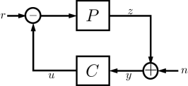
Figure 1: Linear feedback control diagram.

Furthermore, consider the feedback control system illustrated in Fig. 1. In this setup, the reference input $r$ is injected along with the control input $u$ into the system, which produces a controlled output $z$, which the controller $C(\zeta)$, itself a LTI system, attempts to keep small by using knowledge of the system $P$ and noisy measurements $y=z+n$. Through straightforward algebra, one can compute that the true output $z$ of the system $P$ under this feedback interconnection is given by

$$z(\zeta)=P(\zeta)S(\zeta)r(\zeta)-T(\zeta)n(\zeta),\quad S(\zeta):=\frac{1}{1+P(\zeta)C(\zeta)},\quad T(\zeta):=\frac{P(\zeta)C(\zeta)}{1+P(\zeta)C(\zeta)},$$

where $S(\zeta)$ and $T(\zeta)$ are the sensitivity and complementary sensitivity functions (doyle2013feedback) of the feedback interconnection of Fig. 1, respectively. These objects capture the closed-loop maps from reference input $r(\zeta)$ and sensor noise $n(\zeta)$ to the regulated output $z(\zeta)$, and thus through an appropriate quantification of their magnitudes, they can be used as measures of closed-loop performance. One commonly used measure of system magnitude is the $H_{\infty}$-norm.

Definition 2.1.

The $H_{\infty}$ norm of a transfer function $G(\zeta)$ is defined as $\left\|G\right\|_{\infty}=\sup_{\omega\in[-\pi,\pi]}|G(e^{j\omega})|.$

We note that via Parseval’s theorem, the $H_{\infty}$ norm of a system also admits a time-domain interpretation as the worst-case $\ell_{2}\to\ell_{2}$ gain of the filter $G_{t}$ satisfying $\mathcal{Z}(G_{t})=G(\zeta)$, where $\mathcal{Z}$ is the z-transform. As our study focuses on perception-based control, much of our analysis will be focused on characterizing the effects of sensing noise $n(\zeta)$, and hence, the object of concern will be the $H_{\infty}$ norm of the complementary sensitivity function $T(\zeta)$. To that end, we conclude this section with a useful theorem that allows us to lower bound $\left\|T(\zeta)\right\|_{\infty}$ as a function of the open-loop unstable poles and zeros of the system $P(\zeta)$ for any possible controller $C(\zeta)$, thus establishing limits on achievable performance. A proof may be found in Appendix LABEL:ap:limitsProof.

Theorem 2.2 (Ch.6, doyle2013feedback).

Assume that $P(\zeta)$ has unstable poles $p_{k}$ and unstable zeros $q_{k}$, and the interconnection of $P$ with $C$ is internally stable. Then $\left\|T(\zeta)\right\|_{\infty}\geq\max_{i}\prod_{k}\left|\frac{1-p_{i}^{-1}q_{k}^{-1}}{p_{i}^{-1}-q_{k}^{-1}}\right|.$

When $P$ has a single unstable pole and zero, the inequality above simplifies to $\left\|T(\zeta)\right\|_{\infty}\geq\left|\frac{pq-1}{p-q}\right|$. Note that as stated, this bound is valid for SISO LTI systems with linear controllers. There are analogous bounds for multiple-input, multiple-output (MIMO) LTI systems (goodwin2001control) and LTI systems with nonlinear time-varying controllers (khargonekar1986uniformly).

Understanding Limits of Perception-Based Control via Stick Balancing.

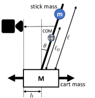
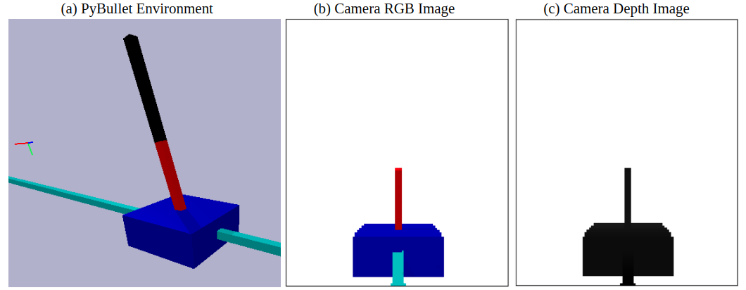
Figure 2: (Left) Schematic of the simplified cartpole system. (Right) Our custom PyBullet environment: (a) a side-on view of the scene to visualize the camera pose with respect to the cartpole system, as well as the occluded portion of the cartpole (in black). (b) RGB image from the camera, (c) depth image from the camera.

We propose using the “stick-balancing” example from (leong2016understanding; doyle2013feedback), shown in Fig. 2 (Left), as a case study. The dynamics of such a one-dimensional inverted pendulum on a moving cart are given by the following second-order ordinary differential equations: