Strong gravitational lensing by rotating Simpson–Visser black holes
Abstract
We investigate strong field gravitational lensing by rotating Simpson-Visser black hole, which has an additional parameter (), apart from mass () and rotation parameter (). A rotating Simpson-Visser metric correspond to (i) a Schwarzschild metric for and , (ii) a Kerr metric for , and (iii) a rotating regular black hole metric for , and in the range , and (iv) a traversable wormhole for a and . We find a decrease in the deflection angle and also in the ratio of the flux of the first image and all other images . On the other hand, angular position increases more slowly and photon sphere radius decreases more quickly, but angular separation increases more rapidly, and their behaviour is similar to that of the Kerr black hole. The formalism is applied to discuss the astrophysical consequences in the supermassive black holes NGC 4649, NGC 1332, Sgr A* and M87* and find that the rotating Simpson-Visser black holes can be quantitatively distinguished from the Kerr black hole via gravitational lensing effects. We find that the deviation of the lensing observables and of rotating Simpson Visser black holes from Kerr black hole for (), for supermassive black holes Sgr A* and M87, respectively, are in the range as and as while is in the range . It is difficult to distinguish the two black holes because the departure are in as), which are unlikely to get resolved by the current EHT observations, and one has to wait for future observations by ngEHT can pin down the exact constraint. We also derive a two-dimensional lens equation and formula for deflection angle in the strong field limit by focusing on trajectories close to the equatorial plane.
I Introduction
That the end state of gravitational collapse of a sufficiently massive star () is a gravitational singularity is a fact established by the singularity theorems of Hawking and Penrose Hawking:1970 (see also Ref. Hawking:1973 ). The existence of a singularity, by its very definition, means spacetime ceases to exist, marking a breakdown of the laws of physics. The extreme condition, in any form, that may exist at the singularity implies that one should rely on quantum gravity which is expected to resolve this singularity Wheeler:1964 . In the absence of any definite quantum gravity, which can allow one to understand the black hole interior and resolve the singularity issue, significant attention shifted to regular models. The idea of regular models was pioneered by Sakharov Sakharov:1966 and Gliner Gliner:1966 , that suggests one can get rid of the singularities by considering a matter, i.e., with a de Sitter core, with the equation of state . The cosmological vacuum obeys this equation of state, and hence, ; is the cosmological constant.
Bardeen Bardeen:1968 , motivated by Sakharov Sakharov:1966 and Gliner Gliner:1966 , proposed the first regular black hole with horizons, but there is no central singularity Ansoldi:2008jw ; Ghosh:2014pba . The Bardeen black hole near the origin acts like the de Sitter spacetime, whereas for large , it is according to Schwarzschild black hole Ansoldi:2008jw . Thus the black hole interior does not result in a singularity but develops a de Sitter like region, eventually settling with a regular center. Thus its maximal extension is the one of the ReissnerNordstrm spacetime, but with a regular center Borde:1994ai ; Borde:1996df . Later, Ayon-Beato and Garcia Ayon:1999 demonstrate that the Bardeen’s model is an exact solution of general relativity coupled to nonlinear electrodynamics thereby an alteration of the ReissnerNordstrm black hole solution Reissner:1916 . There has been an enormous advance in the analysis and application of regular black holes, AyonBeato:1998ub ; Lemos:2011dq ; Cisterna:2020rkc and also on regular rotating black Ghosh:2014pba ; Kumar:2020cve ; Eichhorn:2021etc holes. Most of these solutions are, more or less, based on Bardeen’s proposal that has non-linear electrodynamics as the source. It turns out that most regular black holes have a core that is asymptotical de Sitter (with constant positive curvature) Bardeen:1968 ; AyonBeato:1998ub . One exception is the regular black hole in Refs hc ; Ghosh:2014pba ; Simpson:2019mud has an asymptotically Minkowski core Simpson:2019mud thereby greatly simplifying the physics in the deep core.
Lately, another interesting spherically symmetric regular black hole spacetime is proposed by Simpson-Visser Simpson:2018tsi ; Simpson:2019cer ; Lobo:2020ffi given by
| (1) |
where is a constant with yields the least modification of the Schwarzschild black hole spacetime and encompasses it when . The parameter has dimensions of length introduced to cause a repulsive force to avoid singularity and is responsible for the regularisation of the metric at . This spacetime (1) interpolates between the Schwarzschild black hole and the Morris–Thorne traversable wormhole. The Simpson-Visser metric is regular everywhere; it is evident by analysing the scalar invariant and which are well behaved everywhere including at Simpson:2018tsi . The Simpson-Visser spacetime received significant attention starting with a discussion on the energy conditions, causal structure, and innermost stable circular orbit (ISCO) Simpson:2018tsi . Later, a cascade of work followed, viz. a Vaidya radiating spacetime and traversable wormhole Simpson:2019cer , regularity, quasi-local mass, energy conditions and the causal structure of black bounce models Lobo:2020ffi , gravitational lensing in a strong deflection limit Tsukamoto:2020bjm , construction of rotating counterparts Mazza:2021rgq , the slow rotation generalization and properties of the wormhole branch of this solution Bronnikov:2021liv , and discussion on black holes shadows Junior:2021atr ; Shaikh:2021yux .
The gravitational lensing, one of the earlier predictions of general relativity, is also considered a test of general relativity, primarily being in the strong field regimeCrispino:2019yew . Since then, gravitational lensing proved to be an essential tool for providing insights on the spacetime Einstein:1936yew . In the strong field scenario, the light passes very close to the black hole such that the bending angle is much greater than 1 radian and photon can encircle the black hole more than once which results in shadow Synge:1966 , photon rings Gralla:2019xty , relativistic images Darwin:1959 ; Bozza:2009yw ; Bozza:2001xd ; Bozza:2002zj ; Bozza:2002af . Although relativistic images can not be resolved due to their small separation Virbhadra:1998dy ; Petters:2002fa and thin width Gralla:2019xty , but with the help of the new generation Event Horizon Telescope (ngEHT), they would be accessible and help in distinguishing different kinds of black holes, thus providing a precise test in the strong field limit.
Lately, there has been an enormous discussion of gravitational lensing from the strong field by black holes Virbhadra:1999nm ; Frittelli:1999yf ; Bozza:2001xd ; Bozza:2002zj ; Bozza:2002af ; Bozza:2009yw ; Eiroa:2002mk ; Iyer:2006cn ; Tsukamoto:2016jzh ; Virbhadra:2007kw ; Shaikh:2019jfr , since it could provide another avenue to test general relativity. Virbhadra and Ellis Virbhadra:1999nm have given a numerical recipe that allows studying the large deflection of light rays, resulting in strong gravitational lensing. Later, the strong field gravitational lensing for general spherically symmetric and static spacetime analysed analytically by Bozza in Bozza:2001xd ; Bozza:2002zj ; Bozza:2002af ; Bozza:2009yw and also by Tsukamoto in Tsukamoto:2016jzh . The observationally gravitational lensing by black holes began to be crucial in the 1990s, which triggered quantitative studies of the gravitational lensing by Kerr black holes Bozza:2009yw ; Rauch:1994qd ; Bozza:2008mi . Later, due to the tremendous advancement of current observational facilities, gravitational deflection of light by rotating black holes has received significant attention Ghosh:2020spb ; Wei:2011nj ; Beckwith:2004ae ; Hsiao:2019ohy ; Kapec:2019hro ; Gralla:2019drh ; James:2015yla . In addition, gravitational lensing by hairy Kerr black holes, compared to Kerr black hole, exhibit several interesting feature Cunha:2019ikd . The recent time witnessed significant attention in investing strong gravitational lensing by black holes is due to the EHT results, which released the image of the supermassive M87*. Most galaxies harbour a supermassive black hole in their central region, like M87*, in the elliptical galaxy and the Milky Way has Sagittarius A* Ghez:1998ph .
The goal is to compare the observational predictions of rotating Simpson-Visser black holes with those of the Kerr black hole in an identical observational situation, i.e., same source and observer position and same astrophysical black holes. We only consider an isolated black hole with no surrounding accretion disk or plasma. It is possible that the corrections in the deflection angle, by rotating Simpson-Visser black holes, in the Kerr black holes can be explained by other environmental effects also, such as disk, plasma, dark matter Aldi:2016ntn ; Bozza:2010xqn . A study of deflection of light by Schwarzschild and Kerr black hole in the presence of medium has been presented both in weak and strong field regimes Perlick:2000 ; Tsupko:2013cqa ; Bisnovatyi . Interestingly, the plasma environment around the black hole considerably changes the position and magnification of the relativistic images ZamanBabar:2021aqv . The presence of the uniform plasma around the black hole increases the angular position of the images, and their magnification Tsupko:2013cqa ; Liu:2016eju .
This paper investigates the strong gravitational lensing by rotating Simpson-Visser black holes Mazza:2021rgq and assess the phenomenological differences with the Kerr black holes; in particular, we discuss the effect of deformation parameter on gravitational lensing observables and time delay between the relativistic images. Further, considering the supermassive black holes, NGC 4649, NGC 1332, Sgr A* and M87* as the lens, we obtain the positions, separation, magnification, and time delay in the formation of relativistic images. We have also discuss quasi-equatorial gravitational lensing by rotating Simpson-Visser black holes in the strong field limit. Besides the spin, we also expect to study the influence of the deviation parameter on black hole lensing.
The paper is organized as follows: In the Sec. II, we briefly review the recently obtained rotating Simpson-Visser black holes Mazza:2021rgq and also discuss its horizon structure to put restrictions on parameters and in turn discuss the gravitational deflection of light in the strong field limit for rotating Simpson-Visser black holes Mazza:2021rgq which is the subject in Sect. III. In Sec. III, we also discuss the strong lensing observables by rotating Simpson-Visser black holes, including the image positions , separation , magnifications and time delays of the images. By taking the supermassive black holes NGC 4649, NGC 1332, Sgr A* and M87*, as the lens, we numerically estimate the observables in Sec. IV. In Sec. V we discuss the non-equatorial gravitational lensing and compute the deflection angle in the strong field limit and finally, we summarize our results and evoke some perspectives to end the paper in Sect. VI.
Throughout this paper, unless otherwise stated, we adopt natural units ()
II Rotating Simpson-Visser black holes
The metric of the rotating Simpson-Visser black holes is constructed as a modification from the metric of the Kerr black hole with additional parameter apart from mass and angular momentum , which in Boyer-Lindquist coordinates, reads as Mazza:2021rgq
| (2) | |||||
where , , and . The parameter describes deviation from Kerr black hole and one finds that Kerr black hole is encompassed as a special case (). When , the above metric reduces to the spherical Simpson–Visser metric (1) Simpson:2018tsi ; Simpson:2019cer ; Lobo:2020ffi . When both the parameters and are zero it gives the familiar Schwarzschild solution. The non-negative parameter with dimensions of length is introduced to cause a repulsive force which avoids singularity at . The metric (2), is symmetric under the transformation , and is thus composed of identical portions around . The surface , is a regular surface of finite size for , which the observer can easily cross Mazza:2021rgq . Unlike Bardeen Bardeen:1968 or Hayward spacetimes, metric (2) is either a regular black hole or a traversable worm-hole, depending on the value of the parameter Mazza:2021rgq .
 |
 |
 |
 |
We measure the quantities , and in units of Schwarzschild radius Bozza:2002zj and use instead of radius to rewrite the metric (2) as
| (3) |
where , and .
 |
Interestingly, there exist values of and for which , which correspond to the coordinate singularities. The points of coordinate singularities, if they exist, are also the horizons of the black hole metric (3). Thus, the horizons are located at
| (4) |
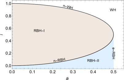
The horizons of the metric (3) exist when and . For , we have two horizons, , corresponding to the radii of outer (event) () and inner (Cauchy) () horizons (This corresponds to RBH-II in Fig 2). Whereas, when , only event horizon exists (This corresponds to RBH-I in Fig 2, also cf. Fig. 1). For and , Cauchy and event horizon correspond to extremal black hole (e-RBH) with degenerate horizons, while for and , there are no horizons and so no black hole. The case with no horizons, the metric (3) describes a traversable wormhole with a time-like throat, which becomes null for Mazza:2021rgq .
We shall be considering only black holes and restrict the values of and in the range and for at least one horizon to exist to qualify the spacetime as a black hole. As the solution is symmetric around , the light deflection will be the same on either side. Without loss of generality, we shall consider . Images are formed on both sides of the lens. We have to carefully choose the correct sign for the angular momentum as all strong field limit coefficients depend on . Conventionally the direction of the black hole spin is in the north. The photons winding counterclockwise are described by a positive and form images on the eastern side of the black hole. Images formed by retrograde rays are described taking a negative and appear on the western side.
The timelike killing vector of the rotating Simpson-Visser metric has norm
| (5) |
becomes positive in the region where For the rotating Simpson-Visser metric, there also exists the static limit surface (SLS) that can be determined by the zeros , i.e., of The region between event horizon and SLS is called ergosphere, where the asymptotic time translation Killing field a becomes spacelike and an observer follow an orbit of .
III Gravitational lensing in strong deflection limit
The rotating Simpson-Visser metric like the Kerr metric has reflection symmetry , due to which the light rays which are initially in the equatorial plane will always remain in the equatorial plane, making it easier to consider the motion of light rays in this plane. Further, we consider the source to be almost aligned along the optical axis, and the source is located behind the lens, which allows the images to be very prominent and highly magnified.
Next, we consider the lens equation given in Bozza:2002zj ; Bozza:2008ev ,
| (6) |
where - , is the extra deflection angle with and . Here, , and are, respectively, the deflection angle, angular separation of source and image from optical axis. The distance of source, lens from the observer are given by and . The lens equation have been used in more general ways Perlick:2003vg ; Eiroa:2003jf ; Frittelli:1998hr ; Frittelli:1999yf but the lens Equation (6) precisely helps to analyse the observational effects. The rotating Simpson-Visser black hole in the equatorial plane () takes the form
| (7) |
where
and and . Using the null geodesic equations which are first order ordinary differential equations Chander:1992pc , the deflection angle of a photon moving on the equatorial plane for rotating Simpson-Visser black hole reads Bozza:2002af
| (8) |
where is the value of at , which is the light’s closest approach. The quantities and are defined in the similar way as and is the projection of angular momentum. Unlike in weak deflection limit, where the deflection angle is minimal and an approximate form can be obtained, in the case of strong deflection limit (SDL), the argument of the integral (8) is expanded near the photon sphere. The photon sphere radius corresponds to the critical impact parameter and is the solution of the following equation Bozza:2002af
| (9) |
which implies
| (10) |
 |
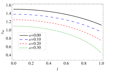 |
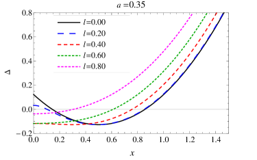
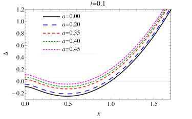
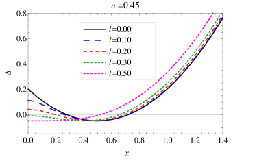
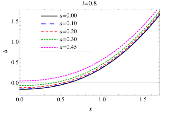
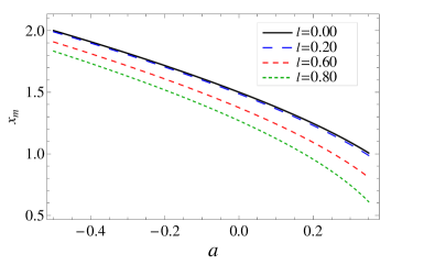
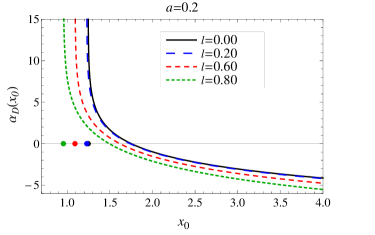
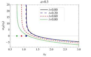
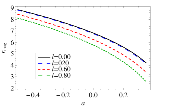
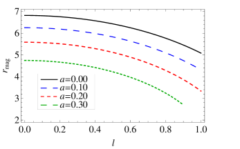
The Eq. (10) is solved numerically and the the radii of photon sphere for the black hole (7) is depicted in Fig. 3 and is smaller when compared with the Kerr black hole (cf. Fig. 3). By assuming the closest distance very near to , the deflection angle when expanded in the SDL takes the form
| (11) |
where is the impact parameter given by
| (12) |
and is the value of impact parameter at and is independent of the parameter (cf. Table 1). Introducing the new variable to obtain the lensing coefficients as Bozza:2002af
| (13) | |||||
| (14) | |||||
| (15) | |||||
| (16) | |||||
| (17) |
 |
 |
 |
 |
| Lensing Coefficients | ||||
| 0.00 | 0.00 | 1.00000 | -0.400230 | 2.59808 |
| 0.25 | 1.01419 | -0.423912 | 2.59808 | |
| 0.50 | 1.06066 | -0.506783 | 2.59808 | |
| 0.75 | 1.15470 | -0.698106 | 2.59808 | |
| 0.95 | 1.29219 | -1.03047 | 2.59808 | |
| 0.15 | 0.00 | 1.14883 | -0.549965 | 2.28260 |
| 0.25 | 1.17017 | -0.587359 | 2.28260 | |
| 0.50 | 1.24212 | -0.723681 | 2.28260 | |
| 0.75 | 1.39860 | -1.071530 | 2.28260 | |
| 0.95 | 1.66148 | -1.79782 | 2.28260 | |
| 0.30 | 0.00 | 1.43692 | -0.891314 | 1.91924 |
| 0.25 | 1.47594 | -0.965136 | 1.91924 | |
| 0.50 | 1.61535 | -1.256170 | 1.91924 | |
| 0.75 | 1.97301 | -2.180740 | 1.91924 | |
| 0.90 | 2.52527 | -4.037170 | 1.91924 | |
| 0.45 | 0.00 | 2.58352 | -2.76735 | 1.42221 |
| 0.30 | 2.79948 | -3.26402 | 1.42221 | |
| 0.40 | 3.01084 | -3.79273 | 1.42221 | |
| 0.50 | 3.3693 | -4.7799 | 1.42221 | |
| 0.60 | 4.05135 | -6.94521 | 1.42221 | |
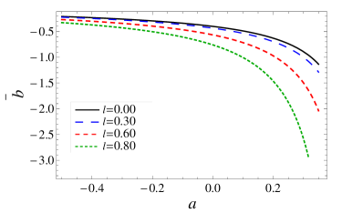
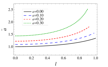
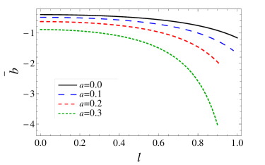
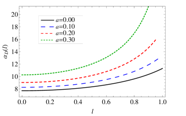
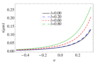
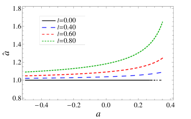
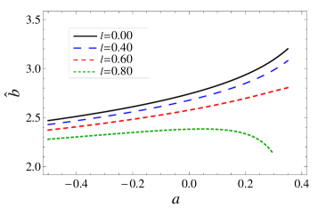
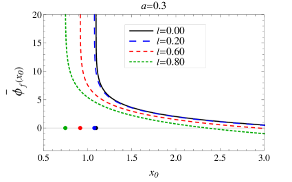
Here the coefficients , are obtained by the Taylor expansion of the term inside the square root of the . The behaviour of coefficients and is shown in Fig. 4, and their behaviour is similar to the Kerr black hole () and spherical Simpson-Visser (). The deflection angle for rotating Simpson-Visser black hole in SDL (cf. Fig 5 and Fig. 6), like Kerr black hole, is more than , and multiple images of the source are formed. The photons that leave the source have to travel through different dispersive medium especially the environment around the black hole e.g the accretion disk, before it reaches the observer. The correction in deflection angle (11) can also be seen as coming from various environmental effects Aldi:2016ntn ; Bozza:2010xqn . It is just that we have not considered all possible sources of corrections such as black hole environment, e.g, accretion or plasma.
|
III.1 Observables
Next we shall estimate the observables for the strong gravitational lensing by rotating Simpson-Visser black hole as in Islam:2021dyk ; Ghosh:2020spb ; Bozza:2002af ; Bozza:2002zj . Using the lens Eq. (6), and following the condition where the source, lens and the observer are aligned, the angular seperation between the lens and the th image is given by Bozza:2002af
| (18) |
where
| (19) | |||||
| (20) | |||||
| (21) |
 |
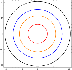
Here is the angular position of the image when a photon encircles complete and the second term in Eq. (18) is the extra term exceeding such that Bozza:2002zj . For perfect alignment, i.e., when , the lens deflects the light equally in all directions such that a ring-shaped image is produced, which are known as Einstein rings Einstein:1936yew . When the lens is exactly halfway between observer and source, the angular radius of the Einstein rings can be obtained by solving Eq. (18) for source, lens, and the observer being perfectly aligned Muller:2008 ; Bozza:2002zj as
| (22) |
where is the angular radius of the outermost Einstein ring (cf. Fig 7) and the Einstein rings produced by the Sgr A* are bigger when compared to other black holes Islam:2021dyk ; Ghosh:2020spb .

|
The surface brightness is preserved in the deflection of the light but the appearance of the solid angle changes thus magnifying the brightness of the images. For the loop images, the magnification is given by Bozza:2002af ; Bozza:2002zj
| (23) |
| Sgr A* | M87* | NGC 4649 | NGC 1332 | |||||
|---|---|---|---|---|---|---|---|---|
| (as) | (min) | (as) | (hrs) | (as) | (hrs) | (as) | (hrs) | |
| 0.00 | 26.3299 | 11.4968 | 19.782 | 289.647 | 14.6615 | 210.328 | 7.76719 | 113.185 |
| 0.15 | 23.1327 | 10.1008 | 17.38 | 254.477 | 12.8812 | 184.789 | 6.82406 | 99.441 |
| 0.30 | 19.4504 | 8.4928 | 14.6133 | 213.968 | 10.8307 | 155.374 | 5.73777 | 83.612 |
| 0.45 | 14.4132 | 6.29295 | 10.8289 | 158.543 | 8.02585 | 115.127 | 4.2518 | 61.9538 |
In the case, , the Eq. (23) diverges, suggesting that the perfect alignment maximises the possibility of the detection of the images. The brightness of the first image is dominant over the other images, and in practice, if the 1-loop image can be distinguished from the rest packed images, we can have three characteristic observables Bozza:2002zj as
| (24) | |||||
| (25) | |||||
| (26) |
In the above expression, is the angular position of the innermost image, is the angular position of the outermost image, is the angular separation between the first image and the inner packed images, is the ratio of the flux of the first image and the all other images. By observationally measuring the , and and inverting the Eqs. (24-26), we can obtain the lensing the coefficients , , the minimum impact parameter as in Islam:2020xmy .
The time travelled by the light paths corresponding to the different images is not the same, and hence there is a time difference between the two images. The time delay, which is another important observable, is defined as the time difference between the formation of relativistic images considering the source with luminosity variations. The time for the photon to travel from the source and to the observer can be obtained using the null geodesic equation as Bozza:2003cp
| (27) |
where we have changed the integration variable from to and split the integral into approach and leaving phase and by exploiting the symmetry between the two phases, we extend the integration to infinity. Finally, if the time signal between the first and second image can be distinguished, the time delay , when they are on the same side of the lens, can be approximated as Bozza:2003cp
| (28) |
where
| (29) |
The essential requirement for measuring the time delay is that the source must be variable, which is not a restrictive requirement as variable stars are abundant in all galaxies. By implicitly assuming these variations, which will show up with a temporal phase in all images, it would be possible to measure the time difference between the relativistic images. From an observational perspective, the precise measurement of the time delay has an important advantage of dimensional measurement of the scale of the system, which can be used to get an accurate estimation of the distance of black hole and possibly to determine the Hubble parameter in cosmological context Refsdal:1964 .
| Sgr A* | M87* | NGC 4649 | NGC 1332 | |||||||
| (as) | (as) | (as) | (as) | (as) | (as) | (as) | (as) | |||
| 0.00 | 0.00 | 26.3628 | 0.0329517 | 19.8068 | 0.0247571 | 14.6799 | 0.0183488 | 7.77691 | 0.00972061 | 6.82188 |
| 0.25 | 26.3652 | 0.0353455 | 19.8086 | 0.0265556 | 14.6812 | 0.0196818 | 7.77762 | 0.0104268 | 6.72647 | |
| 0.50 | 26.3735 | 0.0436767 | 19.8148 | 0.032815 | 14.6858 | 0.0243209 | 7.78008 | 0.0128844 | 6.43173 | |
| 0.75 | 26.3922 | 0.0623325 | 19.8289 | 0.0468314 | 14.6962 | 0.0347092 | 7.78558 | 0.0183878 | 5.90792 | |
| 0.95 | 26.4216 | 0.091705 | 19.8509 | 0.0688993 | 14.7126 | 0.051065 | 7.79425 | 0.0270526 | 5.27931 | |
| 0.15 | 0.00 | 23.1931 | 0.0604049 | 17.4254 | 0.0453831 | 12.9149 | 0.0336359 | 6.84188 | 0.0178192 | 5.93812 |
| 0.25 | 23.198 | 0.0652086 | 17.429 | 0.0489922 | 12.9175 | 0.0363107 | 6.84329 | 0.0192362 | 5.82983 | |
| 0.50 | 23.2148 | 0.0821002 | 17.4417 | 0.0616831 | 12.9269 | 0.0457166 | 6.84828 | 0.0242192 | 5.49214 | |
| 0.75 | 23.2531 | 0.120348 | 17.4704 | 0.0904191 | 12.9482 | 0.0670144 | 6.85956 | 0.0355021 | 4.87764 | |
| 0.95 | 23.3114 | 0.178621 | 17.5142 | 0.134201 | 12.9807 | 0.0994633 | 6.87675 | 0.0526924 | 4.1059 | |
| 0.30 | 0.0 | 19.5823 | 0.131981 | 14.7125 | 0.0991593 | 10.9042 | 0.0734923 | 5.7767 | 0.0389338 | 4.74756 |
| 0.25 | 19.5936 | 0.143258 | 14.721 | 0.107632 | 10.9105 | 0.0797717 | 5.78003 | 0.0422604 | 4.62205 | |
| 0.50 | 19.6331 | 0.18278 | 14.7507 | 0.137326 | 10.9325 | 0.101779 | 5.79169 | 0.0539194 | 4.22317 | |
| 0.75 | 19.717 | 0.266607 | 14.8137 | 0.200306 | 10.9792 | 0.148458 | 5.81642 | 0.078648 | 3.45759 | |
| 0.90 | 19.777 | 0.326616 | 14.8587 | 0.245392 | 11.0126 | 0.181873 | 5.83412 | 0.0963504 | 2.70145 | |
| 0.45 | 0.0 | 14.8471 | 0.433859 | 11.1548 | 0.325965 | 8.26744 | 0.24159 | 4.37982 | 0.127986 | 2.64054 |
| 0.30 | 14.8893 | 0.476064 | 11.1865 | 0.357674 | 8.29094 | 0.265092 | 4.39227 | 0.140437 | 2.43684 | |
| 0.40 | 14.9206 | 0.50742 | 11.21009 | 0.38123 | 8.3084 | 0.28255 | 4.40152 | 0.149689 | 2.26578 | |
| 0.50 | 14.9537 | 0.540453 | 11.2349 | 0.40605 | 8.32679 | 0.30094 | 4.41126 | 0.15943 | 2.02472 | |
| 0.60 | 14.9636 | 0.550440 | 11.2424 | 0.41355 | 8.33235 | 0.306507 | 4.41421 | 0.162377 | 1.15820 | |
 |
 |
 |
 |
 |
 |
 |
 |
IV Applications to supermassive black holes
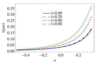
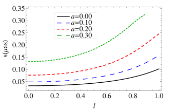
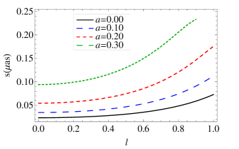
We apply the formalism in the previous section to estimate the observables in SDL by taking the Sgr A*, M87*, NGC4649 and NGC1332 as the rotating Simpson-Visser black holes, and compare them with the corresponding quantities associated with Kerr black hole. The mass and distance from earth for Sgr A* Do:2019vob are , , for M87* Akiyama:2019cqa are , , for NGC4649 Kormendy:2013 are , and for NGC1332 Kormendy:2013 are , , respectively. The observables and for rotating Simpson-Visser black holes for different values of and are depicted in Fig. 8, whereas their values, along with the position of the first image are tabulated in Table 3 and are compared with Schwarzschild black hole () and Kerr black hole (). The observables and time delay do not depend on the parameter and are shown in Table 2. Considering hairy black holes as the lens, we observe that the angular position of first image images for Sgr A* and M87*, is in the range of and , respectively. However, their deviations from the Kerr black hole are not more than as and as, respectively, for . Although they deviate from the Kerr black hole, it is impossible to distinguish the rotating Simpson-Visser black holes from the Kerr black hole using the currently available observation facility of the EHT. Further, the angular separation between the first and inner most image due to the rotating Simpson-Visser black hole for Sgr A* and M87* are in the range of as and as, respectively (cf. Table 3). The angular separation increases with both and suggesting that the image separation is larger than the corresponding Kerr black hole reaching a deviation of as and as for , in case of Sgr A* and M87* respectively, which are beyond the threshold of the current EHT observation (cf. Table 4). We may have to wait for the next generation event horizon telescope (ngEHT) for this purpose. The NGC4649 and NGC1332 show similar behaviour as Sgr A* and M87*, and to conserve space, we have not shown them. If the angular resolution is large enough such that the first image can be resolved from the inner packed ones and it is possible to measure the brightness difference, we find that the of the images decreases with and for rotating Simpson-Visser black hole and thereby its images are less intense than that of Kerr black holes. The angular position and angular separation of the relativistic images, for given values of parameters and , are larger for the Sgr A* black hole than the M87*, NGC4649 and NGC1332 black holes. The time delay of the first image from that of the second image , for Sgr A*, M87*, NGC4649 and NGC1332 respectively, can reach min, hrs, hrs and hrs (cf. Table 2). Thus, the time delay in Sgr A* is much shorter for observation and difficult for measurement. In the case of other black holes, the time delay can reach in the order of a few hundred hours. These are sufficient time for astronomical measurements, provided we have enough angular resolution separating two relativistic images.
| Sgr A* | M87* | NGC 4649 | NGC 1332 | |||||||
|---|---|---|---|---|---|---|---|---|---|---|
| (as) | (as) | (as) | (as) | (as) | (as) | (as) | (as) | |||
| 0.30 | 0.25 | 0.0112769 | 0.0112769 | 0.00803363 | 0.00803363 | 0.00627941 | 0.00627941 | 0.0149856 | 0.0149856 | -0.125517 |
| 0.50 | 0.0507993 | 0.0507993 | 0.0361893 | 0.0361893 | 0.028287 | 0.028287 | 0.0149856 | 0.0149856 | -0.524392 | |
| 0.75 | 0.134626 | 0.134626 | 0.0959075 | 0.0959075 | 0.0749652 | 0.0397141 | 0.0397141 | 0.078648 | -1.28997 | |
| 0.90 | 0.194635 | 0.194635 | 0.138658 | 0.138658 | 0.108381 | 0.0574166 | 0.0574166 | 0.0963504 | -2.04612 | |
| 0.45 | 0.30 | 0.0422 | 0.042205 | 0.0317 | 0.0317098 | 0.0235 | 0.0235018 | 0.0124 | 0.0124505 | -0.2037 |
| 0.40 | 0.0735 | 0.073560 | 0.0552 | 0.0552727 | 0.0409 | 0.0409655 | 0.02170 | 0.0217022 | -0.3747 | |
| 0.50 | 0.1065 | 0.10659 | 0.08008 | 0.0800856 | 0.05935 | 0.0593557 | 0.03144 | 0.0314447 | -0.615823 | |
| 0.60 | 0.1165 | 0.116582 | 0.08758 | 0.0875896 | 0.06491 | 0.0649173 | 0.03439 | 0.0343911 | -0.956684 | |
V Lensing in non-equatorial plane
In the discussion in the previous section on the equatorial plane, we write just a one-dimensional lens equation. However, for practical purposes, e.g., to discuss the caustic structure and find the magnification of the image, it is necessary to consider the two-dimensional lens equation. Thus, it is pertinent to investigate the non-equatorial lensing by rotating Simpson-Visser black hole. We shall analyse the ray trajectories close to the equatorial plane Bozza:2002af of the rotating Simpson-Visser black hole. An additional polar coordinate is required to derive the two-dimensional lens equation so that . Further, the light ray trajectory is identified by three parameters, viz, , and (cf. Fig 9). is the declination that the incoming trajectory makes with the Equatorial plane, is the impact parameter of the projection of the light ray on the Equatorial plane, and lastly, the distance between that point of the projection closer to the black hole and the trajectory is denoted by .
 |
For an observer located at (), two celestial coordinates and can be defined for an image in the Boyer-Lindquist system. Precisely, is the perpendicular distance of the image from the axis of symmetry and is the perpendicular distance of the image from its projection on the equatorial plane. The coordinates and are obtained using the geodesics equations as follows Chander:1992pc ; Bozza:2006nm
| (30) |
Taking into consideration that and , we can relate the constants of motion and to the initial parameters characterising the trajectory, i.e., and as Chander:1992pc ; Bozza:2002af
| (31) |
Here, and are the impact parameters in the non-equatorial planes. The unstable orbit with constant in case of non equatorial orbits is given when and lie on the critical locus. The non equatorial orbits are characterised by , with the value of in between and , which, for the equatorial observer are the radius of the circular orbit for prograde and retrograde respectively.
 |
 |
Following Bozza Bozza:2002af , we restrict our calculation to small inward declination and small height. Accordingly, we write the Eq. (V) up to first order terms as
| (32) |
The evolution of the as a function of azimuthal angle during the motion of the photons around the rotating Simpson-Visser black hole is simply given by
| (33) |
where
| (34) | |||||
| (35) | |||||
| (36) |
The parameter depends on the deviation and spin and reduces to the Kerr black hole case for . Since depends on , the solution of the Eq. (33) is of the form
| (37) |
with
| (38) |
where is the total azimuthal change experienced by the photon and is a constant. The integral in this case can be simplied to
| (39) |
 |
The term is free of singularities and can be absorbed into the function , such that, we can define the quantity which is regular for all values of . Following the same technique we have used for equatorial lensing, Eq. (39) can be expressed in terms of lensing coefficients as
| (40) | |||||
| (41) | |||||
| (42) |
The lensing coefficients and are evaluated at and depicted in Fig. 10. Interestingly, for the case of Kerr black hole we have for all values spin Bozza:2002af . However, for , shows similar behaviour as . On the other tends to increase with for smaller values of , which is contrary to the behaviour of . Variation of is presented in Fig. 11 and as can be seen it tends to zero at slightly higher values of than . The factor for prograde photons and these photons lag the initial declination after each loop while as for retrograde photons and photons tend to lead the initial declination after each loop. Further, we consider the lens geometry by setting the source at some height and the observer at height on the equatorial plane. By assuming that , we can write the polar lens equation as
| (43) |
where and . Solving Eq. (43) for , the inclination and the height for the th image will be
| (44) |
The quantity is the phase of the -th image, which is defined by the Eq. (41) and can be deduced once we obtain the impact angle of -th image using equatorial lens equation. The denominators of terms and can vanish in the neighbourhood of , which defines the position of caustic points.
VI Conclusions
The spacetime singularities in classical general relativity are inevitable, which are also predicted by the celebrated singularity theorems. However, it is a general belief that singularities do not exist in nature, and they are the limitations of general relativity. In the absence of well-defined quantum gravity, models of regular black holes have been studied. Therefore, it is instructive to explore the gravitational lensing to assess the dependence of observables on the parameter and compare the results with those for the Kerr black holes.
With this motivation, we have analyzed the strong gravitational lensing of light due to rotating Simpson-Visser black holes, which besides the mass and angular momentum has an additional deviation parameter . We have examined the effects of the black hole parameter on the light deflection angle and lensing observables , , , , in the strong field observation, due to rotating Simpson-Visser black holes and compare them to the Kerr black holes. We have analytically derived the first order geodesic equations in the background of Simpson-Visser black holes. The observer and source’s geometrical relation has been expressed using an asymptotic lens equation that we combined with geodesic equations to obtain the strong lensing coefficients , and deflection angle. We have numerically calculated the strong lensing coefficients and lensing observables as functions of and for the relativistic images. we find that increases whereas and deflection angle decrease with increasing . depends only on the spin of the black hole and is independent of the black hole parameter . We have calculated the position, separation and relative magnification of these images for supermassive black holes, namely, Sgr A*, M87, NGC 4649 and NGC 1332. Time delay of the first and second image when they are on the same side of the source has also been obtained. The observables and do not depend of . Further, the relative magnification of the first and innermost images is independent of the black hole mass or its distance from the observer. Interestingly, it turns out that the separation between the two relativistic images for Simpson-Visser black holes is greater than that for the Kerr black holes.
The shadow of M87* by EHT is consistent with the Kerr black hole’s image predicted by the GR Akiyama:2019cqa ; Akiyama:2019bqs . Some rotating black holes, arising in modified theories of gravity, are similar to Kerr, with subtle differences on an astrophysical scale. The reported observations do not allow us to rule out these scenarios. Motivated by this also, we investigated the rotating Simpson-Visser black holes, in the strong deflection limit. Although, our results constrain the rotating Simpson-Visser black holes parameter from the gravitational lensing analysis (cf. Figs. 5, 6 and 8) and horizon structure (cf. Figs. 1 and 2). However, the departure produced by the parameter for lensing observables by taking the rotating Simpson-Visser black holes as the supermassive black holes, namely, Sgr A*, M87, NGC 4649 and NGC 1332, from those for Kerr black hole for () are as). Hence, it is difficult to distinguish the regular black holes from the Kerr black hole, at least from the present resolution of astronomical observations like the EHT. Therefore our results, in principle, could provide a possibility to test how rotating Simpson-Visser black holes deviates from the Kerr black hole by future astronomical observations like ngEHT. Our results are the generalization of previous discussions, on the Kerr black holes, in a more general setting.
We have also investigated the non-equatorial (quasi-equatorial) lensing in strong field limit by the rotating Simpson-Visser black hole at very small declination and calculated the deflection angle. An interesting behaviour of is that it goes to unity for all values of spin for the Kerr black hole. , on the other hand, increases with for small values of . The caustic structure not limited to the equatorial plane of rotating Simpson-Visser black holes can help us better understand the phenomenology of the black holes at the centre of our and nearby galaxies, which will be an exciting project.
Many interesting avenues are amenable for future work from the rotating Simpson-Visser solutions; it will be intriguing to analyze the relationship between the null geodesics and thermodynamic phase transition in AdS background in the context photon sphere. One should also see the possibility of generalization of these results to investigate the higher curvature effect in the gravitational lensing. Finally, the possibility of a different conception of these result to gravitational lensing for the solution (2), that describes a wormhole with a throat located at , is an interesting problem for future research. In particular, our results, in the limit , reduced exactly to vis--vis the Kerr black hole results.
It will be intriguing to investigate gravitational lensing in a plasma or accretion environment. Further, the strong field gravitational lensing may open fascinating perspectives for testing modified theories of gravity and estimating the parameters associated with the supermassive black holes.
VII Acknowledgments
S.G.G. and S.U.I. would like to thank SERB-DST for the ASEAN project IMRC/AISTDF/CRD/2018/000042. J.K. would like to thank CSIR for providing JRF. We would like to thank the anonymous reviewer for their valuable comments and suggestions.
References
- (1) S.W. Hawking and R. Penrose, Proc. R. Soc. A 314, 529 (1970).
- (2) S.W. Hawking and G.F.R. Ellis, The Large Scale Structure of Space and Time (Cambridge University Press, Cambridge, 1973).
- (3) J.A. Wheeler, Relativity, Groups, and Topology, edited by C. DeWitt and B. DeWitt (Gordon and Breach, New York, 1964).
- (4) A.D. Sakharov, Sov. Phys. JETP, 22, 241 (1966).
- (5) E.B. Gliner, Sov. Phys. JETP, 22, 378 (1966).
- (6) J. Bardeen, in Proceedings of GR5 (Tiflis, U.S.S.R., 1968).
- (7) S. Ansoldi, [arXiv:0802.0330 [gr-qc]].
- (8) S.G. Ghosh, Eur. Phys. J. C 75, 532 (2015).
- (9) A. Borde, Phys. Rev. D 50, 3692 (1994).
- (10) A. Borde, Phys. Rev. D 55, 7615 (1997).
- (11) E. A. Beato and A. Garcia, Phys. Lett. B 464, 25 (1999); E.A. Beato and A. Garcia, Gen. Relativ. Gravit. 31, 629 (1999).
- (12) H. Reissner, Ann. Phys. 355, 9 (1916).
- (13) E. A. Beato and Alberto Garcia Phys. Rev. Lett. 80, 5056 (1998); S.A. Hayward, Phys. Rev. Lett. 96, 031103 (2006); I. Dymnikova, Gen Relativity Gravity 24, 235 (1992); Z. Y. Fan and X. Wang, Phys. Rev. D 94, 124027 (2016); O.B. Zaslavskii, Phys. Rev. D 80, 064034 (2009).
- (14) J.P.S. Lemos and V.T. Zanchin, Phys. Rev. D 83, 124005 (2011); J. C. S. Neves and A. Saa, Phys. Lett. B 734, 44 (2014); L. Balart and E. C. Vagenas, Phys. Rev. D 90, 124045 (2014); S. G. Ghosh and S. D. Maharaj, Phys. Dark Univ. 31, 100793 (2021); M. S. Ali and S. G. Ghosh, Phys. Rev. D 98, 084025 (2018); A. Kumar, D. Veer Singh and S. G. Ghosh, Eur. Phys. J. C 79, 275 (2019); S. G. Ghosh, Class. Quant. Grav. 35, 085008 (2018).
- (15) A. Cisterna, G. Giribet, J. Oliva and K. Pallikaris, Phys. Rev. D 101, 124041 (2020).
- (16) A. Kumar, S. G. Ghosh and S. D. Maharaj, Phys. Dark Univ. 30, 100634 (2020); R. Kumar, A. Kumar and S. G. Ghosh, Astrophys. J. 896, 89 (2020); R. Kumar and S. G. Ghosh, Class. Quant. Grav. 38, 8 (2021); R. Kumar, S. G. Ghosh and A. Wang, Phys. Rev. D 100, 124024 (2019); R. Kumar and S. G. Ghosh, Astrophys. J. 892, 78 (2020); A. Abdujabbarov, M. Amir, B. Ahmedov and S. G. Ghosh, Phys. Rev. D 93, 104004 (2016); M. Amir and S. G. Ghosh, Phys. Rev. D 94, 024054 (2016); S. G. Ghosh and M. Amir, Eur. Phys. J. C 75, 553 (2015); M. Amir and S. G. Ghosh, JHEP 07, 015 (2015); S. G. Ghosh and S. D. Maharaj, Eur. Phys. J. C 75, 7 (2015); C. Bambi and L. Modesto, Phys. Lett. B 721, 329 (2013).
- (17) A. Eichhorn and A. Held, [arXiv:2103.07473 [gr-qc]]. A. Eichhorn and A. Held, [arXiv:2103.13163 [gr-qc]].
- (18) H. Culetu, Int. J. Theor. Phys. 54, 2855 (2015).
- (19) A. Simpson and M. Visser, Universe 6, 8 (2019).
- (20) A. Simpson and M. Visser, JCAP 02, 042 (2019).
- (21) A. Simpson, P. Martin-Moruno and M. Visser, Class. Quant. Grav. 36, 145007 (2019).
- (22) F. S. N. Lobo, M. E. Rodrigues, M. V. d. S. Silva, A. Simpson and M. Visser, [arXiv:2009.12057 [gr-qc]].
- (23) N. Tsukamoto, Phys. Rev. D 103, 024033 (2021).
- (24) J. Mazza, E. Franzin and S. Liberati, [arXiv:2102.01105 [gr-qc]].
- (25) K. A. Bronnikov, R. A. Konoplya and T. D. Pappas, [arXiv:2102.10679 [gr-qc]].
- (26) H. C. D. L. Junior, L. C. B. Crispino, P. V. P. Cunha and C. A. R. Herdeiro, [arXiv:2102.07034 [gr-qc]].
- (27) R. Shaikh, K. Pal, K. Pal and T. Sarkar, [arXiv:2102.04299 [gr-qc]].
- (28) L. C. B. Crispino and D. Kennefick, Nature Phys. 15, 416 (2019); L. C. B. Crispino and S. Paolantonio, Nature Astron. 4, 6 (2020).
- (29) A. Einstein, Science 84, 506 (1936); S. Liebes, Phys. Rev. 133, B835 (1964); Y. Mellier, Ann. Rev. Astron. Astrophys. 37, 127 (1999); M. Bartelmann and P. Schneider, Phys. Rept. 340, 291(2001); F. Schmidt, Phys. Rev. D 78, 043002 (2008); Guzik, Jacek and Jain, Bhuvnesh and Takada, Masahiro, Phys. Rev. D. 81, 023503 (2010).
- (30) J. L. Synge,Mon. Not. R. Astron. Soc. 131, 463 (1966).
- (31) S. E. Gralla, D. E. Holz and R. M. Wald, Phys. Rev. D 100, 024018 (2019); M. D. Johnson, A. Lupsasca, A. Strominger, G. N. Wong, S. Hadar, D. Kapec, R. Narayan, A. Chael, C. F. Gammie and P. Galison, et al. Sci. Adv. 6, 1310 (2020); S. E. Gralla and A. Lupsasca, Phys. Rev. D 102, 124003 (2020).
- (32) C. Darwin, Proc. R. Soc. A 249, 180 (1959); P. V. P. Cunha and C. A. R. Herdeiro, Gen. Rel. Grav. 50, 42 (2018).
- (33) V. Bozza, Gen. Rel. Grav. 42, 2269 (2010).
- (34) V. Bozza, S. Capozziello, G. Iovane and G. Scarpetta, Gen. Rel. Grav. 33, 1535 (2001).
- (35) V. Bozza, Phys. Rev. D 66, 103001 (2002).
- (36) V. Bozza, Phys. Rev. D 67, 103006 (2003).
- (37) K. S. Virbhadra, D. Narasimha and S. M. Chitre, Astron. Astrophys. 337, 1 (1998).
- (38) A. O. Petters, Mon. Not. Roy. Astron. Soc. 338, 457 (2003).
- (39) K. S. Virbhadra and G. F. R. Ellis, Phys. Rev. D 62, 084003 (2000).
- (40) S. Frittelli, T. P. Kling and E. T. Newman, Phys. Rev. D 61, 064021 (2000).
- (41) E. F. Eiroa, G. E. Romero and D. F. Torres, Phys. Rev. D 66, 024010 (2002)
- (42) S. V. Iyer and A. O. Petters, Gen. Rel. Grav. 39, 1563 (2007).
- (43) N. Tsukamoto, Phys. Rev. D 95, 064035 (2017); N. Tsukamoto and Y. Gong, Phys. Rev. D 95, 064034 (2017).
- (44) K. S. Virbhadra and C. R. Keeton, Phys. Rev. D 77, 124014 (2008).
- (45) R. Shaikh, P. Banerjee, S. Paul and T. Sarkar, JCAP 07, 028 (2019).
- (46) Rauch K P and Blandford R D, Astrophys. J. 46 421 (1994).
- (47) V. Bozza, Phys. Rev. D 78, 063014 (2008).
- (48) S. G. Ghosh, R. Kumar and S. U. Islam, JCAP 03, 056 (2021).
- (49) S. W. Wei, Y. X. Liu, C. E. Fu and K. Yang, JCAP 1210, 053 (2012).
- (50) K. Beckwith and C. Done, Mon. Not. Roy. Astron. Soc. 359, 1217 (2005).
- (51) Y. W. Hsiao, D. S. Lee and C. Y. Lin, Phys. Rev. D 101, 064070 (2020).
- (52) D. Kapec and A. Lupsasca, Class. Quant. Grav. 37, 015006 (2020).
- (53) S. E. Gralla and A. Lupsasca, Phys. Rev. D 101, 044031 (2020).
- (54) O. James, E. von Tunzelmann, P. Franklin and K. S. Thorne, Class. Quant. Grav. 32, 065001 (2015).
- (55) P. Cunha, V.P., C. A. R. Herdeiro and E. Radu, Universe 5, 220 (2019).
- (56) P. V. P. Cunha, C. A. R. Herdeiro and E. Radu, Phys. Rev. Lett. 123, 011101 (2019); P. V. P. Cunha, C. A. R. Herdeiro, E. Radu and H. F. Runarsson, Int. J. Mod. Phys. D 25, 1641021 (2016); P. V. P. Cunha, C. A. R. Herdeiro, E. Radu and H. F. Runarsson, Phys. Rev. Lett. 115, 211102 (2015).
- (57) D. Richstone, E. A. Ajhar, R. Bender, G. Bower, A. Dressler, S. M. Faber, A. V. Filippenko, K. Gebhardt, R. Green and L. C. Ho, et al. Nature 395, A14 (1998).
- (58) A. M. Ghez, B. L. Klein, M. Morris and E. E. Becklin, Astrophys. J. 509, 678 (1998); A. M. Ghez, B. L. Klein, M. Morris and E. E. Becklin, Nature. 419, 694 (2002).
- (59) G. F. Aldi and V. Bozza, JCAP 02, 033 (2017).
- (60) V. Bozza, Gen. Rel. Grav. 42, 2269 (2010).
- (61) V. Perlick, Ray Optics, Fermat’s Principle and Applications to General Relativity : Heidelberg, Germany, (2000).
- (62) O. Y. Tsupko and G. S. Bisnovatyi-Kogan, Phys. Rev. D 87, 124009 (2013).
- (63) G. S. Bisnovatyi-Kogan and O. Y. Tsupko, Plasma Phys. Rep. 41, 562 (2015).
- (64) G. Zaman Babar, F. Atamurotov, S. Ul Islam and S. G. Ghosh, Phys. Rev. D 103, 084057 (2021).
- (65) C. Q. Liu, C. K. Ding and J. L. Jing, Chin. Phys. Lett. 34, 090401 (2017)
- (66) P. Schneider, J. Ehlers, and E. E. Falco, Gravitational Lenses, Springer-Verlag, Berlin (1992).
- (67) A. O. Petters, H. Levine, and J. Wambsganss, Singularity Theory and Gravitational Lensing Birkhauser, Boston (2001).
- (68) K. C. Sahu, J. Anderson, S. Casertano, H. E. Bond, P.Bergeron, E. P. Nelan, L. Pueyo, T. M. Brown, A. Bellini,Z. G. Levay, J. Sokol, M. Dominik, A. Calamida, N. Kains,and M. Livio, Science 356, 1046 (2017).
- (69) T. E. Collett, L. J. Oldham, R. J. Smith, M. W. Auger, K. B.Westfall, D. Bacon, R. C. Nichol, K. L. Masters, K.Koyama, and R. van den Bosch, Science 360, 1342 (2018).
- (70) C. R. Keeton and A. O. Petters, Phys. Rev. D 72, 104006 (2005); C. R. Keeton and A. O. Petters, Phys. Rev. D 73, 044024 (2006); C. R. Keeton and A. O. Petters, Phys. Rev. D 73, 104032 (2006).
- (71) G. Li and X. M. Deng, Annals Phys. 382, 136 (2017).
- (72) K. Akiyama et al. [Event Horizon Telescope], Astrophys. J. Lett. 875, L1 (2019).
- (73) K. Akiyama et al. [Event Horizon Telescope], Astrophys. J. Lett. 875, L4 (2019).
- (74) B. P. Abbott et al., Phys. Rev. Lett. 116, 131103 (2016); B. P. Abbott et al., Phys. Rev. Lett. 116, 241103(2016) ; B. P. Abbott et al.,Phys. Rev. X 6, 041015 (2016).
- (75) V. Perlick, Phys. Rev. D 69, 064017 (2004).
- (76) E. F. Eiroa and D. F. Torres, Phys. Rev. D 69, 063004 (2004).
- (77) S. Frittelli and E. T. Newman, Phys. Rev. D 59, 124001 (1999).
- (78) V. Bozza and L. Mancini, Gen. Rel. Grav. 36, 435 (2004).
- (79) S. Refsdal, MNRAS 128, 307 (1964); R.D. Blandford, R. Narayan, Ann. Rev. Astron. and Astroph. 30, 311 (1992); D. Walsh, R.F. Carswell, R.J. Weymann, Nature 279, 381 (1979).
- (80) J. L. Synge Relativity: The General Theory. North-Holland, Amsterdam, 1960.
- (81) Thomas Muller, Phys. Rev. D 77, 124042 (2008).
- (82) S. U. Islam and S. G. Ghosh, [arXiv:2102.08289 [gr-qc]].
- (83) S. U. Islam, R. Kumar and S. G. Ghosh, JCAP 09, 030 (2020); R. Kumar, S. U. Islam and S. G. Ghosh, Eur. Phys. J. C 80, 1128 (2020).
- (84) S. Chandershaker, The Mathematical Theory of Black Holes, (Oxford University Press. New York, 1992).
- (85) V. Bozza, F. De Luca and G. Scarpetta, Phys. Rev. D 74, 063001 (2006).
- (86) V. Bozza, Phys. Rev. D 78, 103005 (2008).
- (87) Kormendy, John and Ho, Luis C.,Annual Review of Astronomy and Astrophysics 51, 511 (2013).
- (88) T. Do, G. Witzel, A. K. Gautam, Z. Chen, A. M. Ghez, M. R. Morris, E. E. Becklin, A. Ciurlo, M. Hosek, and G. D. Martinez et al.,, Astrophys. J. 882, L27 (2019).