Bayesian Functional Principal Components Analysis via Variational Message Passing

Abstract

Functional principal components analysis is a popular tool for inference on functional data. Standard approaches rely on an eigendecomposition of a smoothed covariance surface in order to extract the orthonormal functions representing the major modes of variation. This approach can be a computationally intensive procedure, especially in the presence of large datasets with irregular observations. In this article, we develop a Bayesian approach, which aims to determine the Karhunen-Loève decomposition directly without the need to smooth and estimate a covariance surface. More specifically, we develop a variational Bayesian algorithm via message passing over a factor graph, which is more commonly referred to as variational message passing. Message passing algorithms are a powerful tool for compartmentalizing the algebra and coding required for inference in hierarchical statistical models. Recently, there has been much focus on formulating variational inference algorithms in the message passing framework because it removes the need for rederiving approximate posterior density functions if there is a change to the model. Instead, model changes are handled by changing specific computational units, known as fragments, within the factor graph. We extend the notion of variational message passing to functional principal components analysis. Indeed, this is the first article to address a functional data model via variational message passing. Our approach introduces two new fragments that are necessary for Bayesian functional principal components analysis. We present the computational details, a set of simulations for assessing accuracy and speed and an application to United States temperature data.

1 Introduction

Functional principal components analysis (FPCA) is the methodological extension of classical principal components analysis (PCA) to functional data. Within the overarching framework of functional data analysis, FPCA is a central technique. The advantages of using FPCA for functional data are derived from analogous advantages that PCA affords for multivariate data analysis. For instance, PCA in the multivariate data setting is used to reduce dimensionality and identify the major modes of variation of the data set. The modes of variation are determined by the eigenvectors of the sample covariance matrix of the data set, while dimension reduction is achieved by identifying the eigenvectors that maximize variation in the data. In the functional setting, response curves are interpreted as independent realisations of an underlying stochastic process. A covariance operator and its eigenfunctions play the analogous role that the covariance matrix and its eigenvectors play in the multivariate data setting. By identifying the eigenfunctions with the largest eigenvalues, one can reduce the dimensionality of the entire data set by approximating each curve as a linear combination of the reduced set of eigenfunctions.

There are technical issues that arise in the functional setting that are not present for multivariate data. The domain of the functional curves is typically a compact interval $[0,T]$ of the real line. Despite having a continuous domain, the curves are only observed at discrete points over this interval. Furthermore, the points of observation, as well as the total number of observations, need not be the same for each curve. Therefore, approaches that are used in PCA require modifications to extend to the functional framework. In FPCA, we often rely on nonparametric regression to smooth the eigenfunctions and employ an appropriate step to ensure that they are orthonormal from the perspective of integration, rather than inner products of vectors.

There have been numerous developments in FPCA methodology throughout the statistical literature. A thorough introduction to the statistical framework and applications can be found in [Chapter 8]ramsay05 and [Section 2]wang16. Much of this work mirrors the eigendecomposition approach to PCA, in that an eigenbasis is obtained from a covariance surface. yao05 focused on the case of sparsely observed functional data, and estimate principal component scores through conditional expectations. xiao16 developed a fast covariance estimation method for densely observed functional data. di09 extended FPCA to multilevel functional data, extracting within and between subject sources of variability, and greven2011 developed methods for longitudinal functional data. However, goldsmith13 noted that these approaches implicitly condition on an estimated eigenbasis to estimate scores, meaning that inference on individual curve estimates can be inaccurate.

Meanwhile, other approaches have built on or are similar to the probabilistic PCA framework that was introduced by tipping99 and bishop99. Rather than first obtaining eigenfunctions from a covariance and then estimating scores, all quantities are considered unknown and are estimated jointly. james2000 used an EM algorithm for estimation and inference in the context of sparsely observed curves. Variational Bayes for FPCA was introduced by vanderlinde08 via a generative model with a factorized approximation of the full posterior density function. Goldsmith15 introduced a fully Bayes framework for multilevel function-on-scalar regression models, and also considered observed values that arise from exponential family distributions.

In frequentist versions of FPCA, the covariance function is determined through bivariate smoothing of the raw covariances. Eigenfunctions and eigenvalues are then determined from the smoothed covariance function. The key advantage in the Bayesian approach is that the covariance function is not estimated, meaning that complex bivariate smoothing is not required. Indeed, the eigenfunctions and eigenvalues are computed directly as part of a Bayesian hierarchical model. Furthermore, it is unnecessary to compute or store large covariance matrices for dense functional data, and for sparse, irregular functional data – where estimating the raw covariance is difficult or impossible – direct estimation of eigenfunctions in a Bayesian model is straightforward. For these reasons, we pursue a Bayesian approach to FPCA.

Although there have been numerous contributions to Bayesian implementations of FPCA, we argue that there are additional considerations that should be addressed. First, MCMC modeling of FPCA is a computationally expensive procedure and, in some biostatistical applications Goldsmith15, the computational time can reach several hours. Second, current versions of variational Bayes for FPCA, despite being a much faster computational alternative, are difficult to extend to more complex likelihood specifications, such as multilevel data models and binary response outcomes.

minka05 presents a unifying view of approximate Bayesian inference under a message passing framework that relies on the notion of messages passed between nodes of a factor graph. Mean field variational Bayes (MFVB) can be incorporated into this framework through an alternate scheme known as variational message passing (VMP) winn05. wand17 introduced computational units, known as fragments, that compartmentalize the algebraic derivations that are necessary for approximate Bayesian inference in VMP. The notion of fragments within a factor graph is essential for efficient extensions of variational Bayes-based FPCA to arbitrarily large statistical models.

In this article, we propose an FPCA extension of the VMP framework for variational Bayesian inference set out in wand17. Our novel methodology includes the introduction of two fragments that are necessary for computing approximate posterior density functions under an MFVB scheme, as well as a sequence of post-processing steps for estimating the orthonormal eigenfunctions. We provide an introduction to variational Bayesian inference in Section 2, with an overview of VMP in Section 2.2. Section 3 introduces the Bayesian hierarchical model for FPCA and its extensions under a VMP formulation. In Section 4, we outline the post-VMP steps that are required for producing orthonormal eigenfunctions. Simulations, including speed and accuracy comparisons with MCMC algorithms, are presented in Section 5, and an application to United States temperature data is provided in Section 6.

2 Variational Bayesian Inference

The overarching aim of this article is the identification and derivation of fragments that are necessary for VMP implementations of FPCA. VMP represents a class of methodologies, derived from MFVB approaches, for approximate Bayesian inference over a factor graph. In this section, we provide a brief introduction to the MFVB and VMP frameworks. For an in-depth explanation of MFVB, we refer the reader to ormerod10 and blei17; for a comprehensive review of VMP, we refer the reader to minka05 and wand17.

Variational Bayesian inference is based on the notion of minimal Kullback-Leibler divergence to approximate a posterior density function. For arbitrary density functions $p_{1}$ and $p_{2}$ on $\R^{d}$, the Kullback-Leibler divergence of $p_{1}$ from $p_{2}$ is

$$\DKL(p_{1},p_{2})\equiv\bigintsss_{\R^{d}}\log\left\{\frac{p_{1}(\bx)}{p_{2}(\bx)}\right\}p_{1}(\bx)d\bx.$$

Note that

$$\DKL(p_{1},p_{2})\geq 0.$$ (1)

Consider a generic Bayesian model with observed data vector $\by$ and parameter vector $\btheta\in\Theta$, where $\bTheta$ is a parameter space. We make the assumption that $\by$ and $\btheta$ are continuous random variables with density functions $p(\by)$ and $p(\btheta)$. For the case where some components are discrete, a similar treatment applies with summations replacing integrals. Next, let $q(\btheta)$ represent an arbitrary density function over the parameter space $\Theta$. The essence of variational Bayesian inference is to restrict $q$ to a class of density functions $\Qsc$ and use the optimal $q$-density function, defined by

$$q^{*}(\btheta)\equiv\argmin_{q\in\Qsc}\ \DKL\{q(\btheta),p(\btheta|\by)\},$$ (2)

as an approximation to the true posterior density function $p(\btheta|\by)$.

Simple algebraic arguments <e.g.>[Section 2.1]ormerod10 show that the marginal log-likelihood satisfies:

$$\log p(\by)=\DKL\{q(\btheta),p(\btheta|\by)\}+\log\underline{p}(\by;q),$$

where

$$\underline{p}(\by;q)\equiv\exp\left[\bigintsss\log\left\{\frac{p(\by,\btheta)}{q(\btheta)}\right\}q(\btheta)d\btheta\right].$$

From the non-negativity condition of (1), we have

$$\underline{p}(\by;q)\leq p(\by)$$

showing that $\underline{p}(\by;q)$ is a lower-bound on the marginal likelihood. This leads to an equivalent form for the optimisation problem in (2):

$$q^{*}(\btheta)\equiv\argmax_{q\in\Qsc}\{\log\underline{p}(\by;q)\}.$$ (3)

As stated in rohde16, this alternate expression has the advantage of representing the optimal $q$-density function as maximising the lower-bound on the marginal log-likelihood. For the remainder of this article, we will address variational Bayesian inference with (3), rather than (2).

2.1 Mean Field Variational Bayes

MFVB is a class of variational Bayesian inference methods that uses a product density (or mean field) restriction in the optimal $q$-density function. The mean field approximation, which has its roots in statistical physics parisi88, imposes the factorization

$$q(\btheta)=\prod_{i=1}^{N}q(\btheta_{i}),$$ (4)

for all $q\in\Qsc$, where $\{\btheta_{1},\dots,\btheta_{N}\}$ is some partition of $\btheta$. The optimal $q$-density functions that satisfy (3) are given by <e.g.>minka05, ormerod10

$$q^{*}_{i}(\btheta_{i})=\frac{\exp\{\E_{q(\btheta\setminus\btheta_{i})}\log p(\by,\btheta)\}}{\int\exp\{\E_{q(\btheta\setminus\btheta_{i})}\log p(\by,\btheta)\}d\btheta_{i}},\quad\text{for $i=1,\dots,N$,}$$ (5)

where $\E_{q(\btheta\setminus\btheta_{i})}$ denotes expectation with respect to the optimal posterior density functions of all elements in the partition of $\btheta$, defined by (4), except for the optimal posterior density function of $\btheta_{i}$.

The parameter vectors that define each of the optimal $q$-density functions in (5) are interrelated and are updated by a coordinate ascent algorithm (ormerod10, Algorithm 1). However, the resulting parameter vector updates are problem-specific and must be rederived if there is a change to the model. For instance, the updates for the optimal posterior density functions of the coefficients in a linear regression model will differ from those in a linear logistic regression model.

2.2 Variational Message Passing

VMP is an alternate computational framework for variational Bayesian inference with a mean field product restriction. The VMP infrastructure is a factor graph representation of the Bayesian model. wand17 advocates for the use of fragments, a sub-graph of a factor graph, as a means of compartmentalizing the algebra and computer coding required for variational Bayesian inference. Posterior density estimation is achieved by messages passed within and between factor graph fragments. Here, we give a brief description of the foundations of VMP. For a thorough exposition of the VMP framework, we refer the reader to wand17.

Consider a generic Bayesian model with observed data vector $\by$ and parameter vectors $\btheta_{1},\dots,\btheta_{5}$. Suppose that the joint density function factorizes according to

$$p(\by,\btheta_{1},\dots,\btheta_{5})=p(\by|\btheta_{1},\btheta_{2},\btheta_{3})p(\btheta_{1})p(\btheta_{2}|\btheta_{4},\btheta_{5})p(\btheta_{3}|\btheta_{4})p(\btheta_{4})p(\btheta_{5}).$$ (6)

A factor graph representation of the Bayesian model expressed in (6) is presented in Figure 1. The square nodes are the factors, which represent the distributional specifications of the model, and the circular nodes are called stochastic nodes, which represent the parameter vectors of the model. Furthermore, the graph is bipartite, meaning that stochastic nodes can only share an edge with a factor and vice versa. Additionally, notice that the edges of the factor graph respect the distributional dependencies of (6). For instance, the factor for $p(\btheta_{2}|\btheta_{4},\btheta_{5})$ shares edges with the stochastic nodes for $\btheta_{2}$, $\btheta_{4}$ and $\btheta_{5}$ only.

Figure 1: A factor graph representation of the Bayesian model described by (6). As an example, the factor graph fragment for $p(\btheta_{2}|\btheta_{4},\btheta_{5})$ is highlighted in blue.

The VMP construction of variational Bayesian inference relies on messages passed between factors and stochastic nodes. Consider the factor for $p(\btheta_{2}|\btheta_{4},\btheta_{5})$ and the messages that it will pass to its neighboring stochastic nodes $\btheta_{2}$, $\btheta_{4}$ and $\btheta_{5}$. The messages passed from this factor are updated according to

$$\msg{p(\btheta_{2}|\btheta_{4},\btheta_{5})}{\btheta_{i}}(\btheta_{i})\longleftarrow\frac{\E_{q(\btheta\setminus\btheta_{i})}\log p(\btheta_{2}|\btheta_{4},\btheta_{5})}{\int\E_{q(\btheta\setminus\btheta_{i})}\log p(\btheta_{2}|\btheta_{4},\btheta_{5})d\btheta_{i}},\quad\text{for $i=2,4,5$.}$$ (7)

Before continuing, we will make a brief note on our notation for computational updates. In (7), we use a left arrow to indicate a computational update, rather than an equality symbol. This reflects the fact that at each iteration of the VMP algorithm, the algebraic form of the message remains the same, whereas the parameter values of the message will change between iterations as the Kullback-Leibler divergence is minimized. In addition, the subscript of the message in (7) indicates the direction of the message. Finally, each message is a function of the parameter vector that it is sent to or sent from.

Next, consider the stochastic node $\btheta_{4}$, which receives messages from the factors $p(\btheta_{2}|\btheta_{4},\btheta_{5})$, $p(\btheta_{3}|\btheta_{4})$ and $p(\btheta_{4})$. The messages that $\btheta_{4}$ returns to these factors are

$$\begin{split}\msg{\btheta_{4}}{p(\btheta_{2}|\btheta_{4},\btheta_{5})}(\btheta_{4})&\longleftarrow\msg{p(\btheta_{3}|\btheta_{4})}{\btheta_{4}}(\btheta_{4})\ \msg{p(\btheta_{4})}{\btheta_{4}}(\btheta_{4})\\ \msg{\btheta_{4}}{p(\btheta_{3}|\btheta_{4})}(\btheta_{4})&\longleftarrow\msg{p(\btheta_{2}|\btheta_{4},\btheta_{5})}{\btheta_{4}}(\btheta_{4})\ \msg{p(\btheta_{4})}{\btheta_{4}}(\btheta_{4})\\ \msg{\btheta_{4}}{p(\btheta_{4})}(\btheta_{4})&\longleftarrow\msg{p(\btheta_{2}|\btheta_{4},\btheta_{5})}{\btheta_{4}}(\btheta_{4})\ \msg{p(\btheta_{3}|\btheta_{4})}{\btheta_{4}}(\btheta_{4}).\end{split}$$ (8)

In general, the message that a stochastic node passes to a neighbouring factor is simply the product of the messages that it has received from its other neighbouring factors. Note that the form of the message updates in (7) are such that the range of each message is a subset of $\R$. Therefore, the computations in (8) simply involve multiplication of scalars.

Now, consider a general Bayesian model with $M$ factors $p_{1},\dots,p_{M}$ and $N$ parameter vectors $\btheta_{1},\dots,\btheta_{N}$. We define the set of stochastic nodes that are connected to the factor $p_{j}$ as

$$\neighbors(j)\equiv\{i=1,\dots,N:\text{$\btheta_{i}$ shares an edge with $p_{j}$}\}.$$

Then, the message from factor $p_{j}$ to the stochastic node $\btheta_{i}$ is

$$\msg{p_{j}}{\btheta_{i}}(\btheta_{i})\longleftarrow\frac{\E_{q(\btheta\setminus\btheta_{i})}\log p_{j}}{\int\E_{q(\btheta\setminus\btheta_{i})}\log p_{j}d\btheta_{i}}.$$ (9)

The message from $\btheta_{i}$ to $p_{j}$ is

$$\msg{\btheta_{i}}{p_{j}}(\btheta_{i})\longleftarrow\prod_{j^{\prime}\neq j:i\in\neighbors(j^{\prime})}\msg{p_{j^{\prime}}}{\btheta_{i}}(\btheta_{i}).$$ (10)

Upon convergence of the messages, the optimal $q$-density functions, which satisfy (3) take the form

$$q^{*}(\btheta_{i})\propto\prod_{j:i\in\neighbors(j)}\msg{p_{j}}{\btheta_{i}}(\btheta_{i}),\quad i=1,\dots,N.$$ (11)

The VMP iterative loop has the following generic steps minka05; wand17:

1. Choose a factor.

2. Update the messages passed from the factor’s neighbouring stochastic nodes to the factor.

3. Update the messages passed from the factor to its neighbouring stochastic nodes.

2.2.1 Exponential Family Form

A key step in deriving and implementing VMP algorithms is the representation of probability density functions in exponential family form. In particular, the messages in (9) and (10) are typically in the exponential family of density functions with vector of sufficient statistics $\bT(\btheta_{i})$. We have

$$\msg{p_{j}}{\btheta_{i}}(\btheta_{i})\propto\exp\{\T{\bT(\btheta_{i})}\np{p_{j}}{\btheta_{i}}\},\quad\text{and}\quad\msg{\btheta_{i}}{p_{j}}(\btheta_{i})\propto\exp\{\T{\bT(\btheta_{i})}\np{\btheta_{i}}{p_{j}}\},$$

where $\np{p_{j}}{\btheta_{i}}$ and $\np{\btheta_{i}}{p_{j}}$ are the message natural parameter vectors. wand17 explains how natural parameter vectors play a central role in the messages that are passed within and between factor graph fragments. Furthermore, the natural parameter vectors for the optimal $q$-density functions in (11) take the form

$$\npq{\btheta_{i}}=\sum_{j:i\in\neighbors(j)}\np{p_{j}}{\btheta_{i}},\quad i=1,\dots,N.$$ (12)

In addition, we adopt the notation

$$\npbf{p_{j}}{\btheta_{i}}\equiv\np{p_{j}}{\btheta_{i}}+\np{\btheta_{i}}{p_{j}}.$$ (13)

Before introducing the exponential family forms for key distributions in the VMP setting, we outline some matrix and vector operators. We define the $\vect$ and $\vech$ operators, which are well-established <e.g.>gentle07. For a $d_{1}\times d_{2}$ matrix, the $\vect$ operator concatenates the columns of the matrix from left to right. For a $d_{1}\times d_{1}$ matrix, the $\vech$ operator concatenates the columns of the matrix after removing the above diagonal elements. For example, suppose that

$$\bA=\begin{bmatrix}2&-1\\ -3&1\end{bmatrix}.$$

Then $\vect(\bA)=\T{(2,-3,-1,1)}$ and $\vech(\bA)=\T{(2,-3,1)}$. For a $d^{2}\times 1$ vector $\ba$, $\vect^{-1}(\ba)$ is the $d\times d$ matrix such that $\vect\{\vect^{-1}(\ba)\}=\ba$. Additionally, the matrix $\bD_{d}$ is the duplication matrix of order $d$, and it is such that $\bD_{d}\vech(\bA)=\vect(\bA)$ for a $d\times d$ symmetric matrix $\bA$. Furthermore, $\bD_{d}^{+}\equiv(\T{\bD_{d}}\bD_{d})^{-1}\T{\bD_{d}}$ is the Moore-Penrose inverse of $\bD_{d}$, where $\bD_{d}^{+}\vect(\bA)=\vech(\bA)$.

The normal distribution is one of the most important distributions within the exponential family, and it plays a major role in VMP versions of variational Bayesian inference. Consider the $d\times 1$ multivariate normal random vector $\bx\sim\normal(\bmu,\bSigma)$. The probability density function of $\bx$ can be shown to satisfy

$$p(\bx)=\exp\left\{\T{\bT_{\vect}(\bx)}\bdeta_{\vect}-A_{\vect}(\bdeta_{\vect})-\frac{d}{2}\log(2\pi)\right\}$$ (14)

where

$$\bT_{\vect}(\bx)\equiv\begin{bmatrix}\bx\\ \vect(\bx\T{\bx})\end{bmatrix}\quad\text{and}\quad\bdeta_{\vect}\equiv\begin{bmatrix}\bdeta_{\vect,1}\\ \bdeta_{\vect,2}\end{bmatrix}\equiv\begin{bmatrix}\bSigma^{-1}\bmu\\ -\frac{1}{2}\vect(\bSigma^{-1})\end{bmatrix}$$

are, respectively, the vector of sufficient statistics and the natural parameter vector. The function

$$A_{\vect}(\bdeta_{\vect})=-\frac{1}{4}\T{\bdeta}_{\vect,1}\left\{\vect^{-1}(\bdeta_{\vect,2})\right\}^{-1}\bdeta_{\vect,1}-\frac{1}{2}\log\left|-2\vect^{-1}(\bdeta_{\vect,2})\right|$$

is the log-partition function. The inverse mapping of the natural parameter vector is (wand17, equation S.4)

$$\bmu=-\frac{1}{2}\left\{\vect^{-1}(\bdeta_{\vect,2})\right\}^{-1}\bdeta_{\vect,1}\quad\text{and}\quad\bSigma=-\frac{1}{2}\left\{\vect^{-1}(\bdeta_{\vect,2})\right\}^{-1}.$$ (15)

We will refer to the representation of the multivariate normal probability density function in (14) as the vec-based representation. Alternatively, a more storage-economical representation of the multivariate normal probability density function is the vech-based representation:

$$p(\bx)=\exp\left\{\T{\bT_{\vech}(\bx)}\bdeta_{\vech}-A_{\vech}(\bdeta_{\vech})-\frac{d}{2}\log(2\pi)\right\},$$

where the vector of sufficient statistics, the natural parameter vector and the log-partition function are, respectively,

$$\bT_{\vech}(\bx)\equiv\begin{bmatrix}\bx\\ \vech(\bx\T{\bx})\end{bmatrix},\quad\bdeta_{\vech}\equiv\begin{bmatrix}\bdeta_{\vech,1}\\ \bdeta_{\vech,2}\end{bmatrix}\equiv\begin{bmatrix}\bSigma^{-1}\bmu\\ -\frac{1}{2}\T{\bD_{d}}\vect(\bSigma^{-1})\end{bmatrix}$$

and

$$A_{\vech}(\bdeta_{\vech})=-\frac{1}{4}\T{\bdeta}_{\vech,1}\left\{\vect^{-1}(\bD_{d}^{+\intercal}\bdeta_{\vech,2})\right\}^{-1}\bdeta_{\vech,1}-\frac{1}{2}\log\left|-2\vect^{-1}(\bD_{d}^{+\intercal}\bdeta_{\vech,2})\right|.$$

The inverse mapping of the natural parameter vector under the vech-based representation is

$$\bmu=-\frac{1}{2}\left\{\vect^{-1}(\bD_{d}^{+\intercal}\bdeta_{\vech,2})\right\}^{-1}\bdeta_{\vech,1}\quad\text{and}\quad\bSigma=-\frac{1}{2}\left\{\vect^{-1}(\bD_{d}^{+\intercal}\bdeta_{\vech,2})\right\}^{-1}.$$ (16)

The other major distribution within the exponential family that is pivotal for this article is the inverse-$\chi^{2}$ distribution. A random variable $x$ has an inverse-$\chi^{2}$ distribution with shape parameter $\xi>0$ and scale parameter $\lambda>0$ if the probability density function of $x$ is

$$p(x)=\frac{(\lambda/2)^{\xi/2}}{\Gamma(\xi/2)}x^{-(\xi+2)/2}\exp\left(-\frac{\lambda}{2x}\right)\ind(x>0),$$

where $\Gamma(\cdot)$ is the gamma function defined by $\Gamma(z)\equiv\int_{0}^{\infty}u^{z-1}e^{u}du$. The exponential family representation of the inverse-$\chi^{2}$ density function is

$$p(x)=\exp\left\{\T{\bT(x)}\bdeta-A(\bdeta)\right\}\ind(x>0),$$

where the vector of sufficient statistics, the natural parameter vector and the log-partition function are, respectively,

$$\bT(x)\equiv\begin{bmatrix}\log(x)\\ 1/x\end{bmatrix}\quad\text{and}\quad\bdeta\equiv\begin{bmatrix}\eta_{1}\\ \eta_{2}\end{bmatrix}\equiv\begin{bmatrix}-\frac{1}{2}(\xi+2)\\ -\frac{\lambda}{2}\end{bmatrix}$$

and

$$A(\bdeta)\equiv\log\{\Gamma(\xi/2)\}-\frac{\xi}{2}\log(\lambda/2).$$

The inverse mapping of the natural parameter vector is (maestrini20, equation 8)

$$\xi=-2\eta_{1}-2\quad\text{and}\quad\lambda=-2\eta_{2}.$$

The generalization of the inverse-$\chi^{2}$ distribution is the inverse G-Wishart distribution, written $\bX\sim\igw(G,\xi,\Lambda)$, for a symmetric and positive definite $d\times d$ matrix $\bX$. The parameter $G$ is an undirected graph with $d$ nodes and edge set $E$ with pairs of nodes connected by an edge. Furthermore, $\xi>0$ and $\bLambda$ is a symmetric and positive definite $d\times d$ matrix. We say that, the symmetric matrix $\bA$ respects $G$ if $\bA_{ij}=0$ for all $(i,j)\notin E$. Now, impose the additional constraint that $\bX^{-1}$ respects $G$. Furthermore, let $G_{\text{full}}$ represent a complete graph where each node is connected to every other node by an edge, and let $G_{\text{diag}}$ represent a sparse graph where the edge set is empty. The justification for this notation is that a matrix with no zero constraints respects $G_{\text{full}}$ and a diagonal matrix respects $G_{\text{diag}}$. The two graph constructions generate two definitions for the inverse G-Wishart distribution (maestrini20, Definition 3):

1. If $G=G_{\text{full}}$ and $\xi$ is restricted such that $\xi>2d-2$ then we say that $\bX$ has an inverse G-Wishart distribution with graph $G$, shape parameter $\xi$ and scale matrix $\bLambda$ if and only if the non-zero values of the density function of $\bX$ satisfy

   $$p(\bX)\propto|\bX|^{-(\xi+2)/2}\exp\left\{-\frac{1}{2}\tr(\bLambda\bX^{-1})\right\}$$

2. If $G=G_{\text{diag}}$, then we say the $\bX$ has an inverse G-Wishart distribution with graph $G$, shape parameter $\xi>0$ and scale matrix $\bLambda$ if and only if the non-zero values of the density function of $\bX$ satisfy

   $$p(\bX)\propto|\bX|^{-(\xi+2)/2}\exp\left\{-\frac{1}{2}\tr(\bLambda\bX^{-1})\right\}.$$

The exponential family form of the inverse G-Wishart distribution is not important for this article; we refer the reader to [Section 2.2]maestrini20. Instead, our interest lies in the role of the graphical parameter, which must be incorporated as an argument for variational message updates involving inverse G-Wishart random matrices, including inverse-$\chi^{2}$ random variables. We follow the advice in [Sections 5 & 6]maestrini20 for message passing updates involving graphical parameters.

2.2.2 Factor Graph Fragments

A factor graph fragment (or fragment, for short) is the computational unit of VMP. A fragment, as defined by wand17, is a subgraph of a factor graph consisting of a single factor and each of its neighboring stochastic nodes. An example of a factor graph fragment is the fragment for $p(\btheta_{2}|\btheta_{4},\btheta_{5})$ in Figure 1, which is highlighted in blue. The factor representing $p(\btheta_{2}|\btheta_{4},\btheta_{5})$, the neighboring stochastic nodes $\btheta_{2}$, $\btheta_{4}$ and $\btheta_{5}$ and the connecting edges comprise the fragment.

The identification and derivation of the algebraic computations in fragments is the key step for extending VMP to arbitrarily large Bayesian statistical models. As explained at the end of Section 2.1, the form of each of the optimal $q$-density functions is problem-specific, requiring rederivations for any changes in the model. However, the fragment based approach in VMP means that updates are localized within the fragment. This represents enormous savings in algebraic derivations and coding because once a fragment has been coded and stored, it can simply be called as a function without the need to rederive the updates. Any change in the model is simply handled by removing the fragment that does not fit the new model and replacing it with an appropriate alternative.

The following is a list of some of the major contributions to fragment updates for VMP:

• wand17 identified five fundamental fragments for Gaussian response semiparametric regression. This includes the Gaussian prior fragment, inverse G-Wishart prior fragment and the iterated inverse G-Wishart fragment, which are necessary for a VMP construction of Bayesian FPCA. The author also identified several other fragments for direct implementation in various extensions for semiparametric regression.

• nolan17 developed fast, stable and accurate numerical integration techniques for the logistic likelihood fragment. This had been previously introduced in wand17 using the variational lower bound of jaakkola00, however the performance of this approximation can be poor knowles11. Instead, nolan17 incorporated the normal scale mixture uniform approximation of the logistic function monahan92 into the logistic likelihood fragment for highly accurate inference.

• maestrini18 derived algorithmic updates for the skew $t$ likelihood fragment with all skew $t$ parameters inferred, rather than being held fixed.

• mclean19 built on previous VMP constructions by focusing on regression models where the response variable is modeled to have an elaborate distribution, such as Negative Binomial and $t$ likelihoods.

• nolanmw20 used a set of solutions to sparse multilevel matrix problems nolan19 to streamline the computations of VMP for Gaussian response linear mixed models. This involved the introduction of four new fragments.

• maestrini20 provide corrections for the matrix versions of the inverse G-Wishart prior fragment and the iterated inverse G-Wishart fragment from wand17. In particular, Section 4.1.3 of wand17, which introduces the iterated inverse G-Wishart fragment, only addresses the case where the graph parameter is $G=G_{\text{full}}$. However, it does not account for the case where $G=G_{\text{diag}}$. The necessary corrections are outlined in Section 6.1 of maestrini20. Although the scalar versions of these fragments from wand17 are sufficient for the current article, we will use the updated fragments from maestrini20 since they are the new standard for approximate Bayesian inference on variance and covariance matrix parameters.

3 Functional Principal Components Analysis

Consider a random sample of i.i.d. smooth random functions $y_{1},\dots,y_{n}\in L^{2}[0,1]$. We will assume the existence of a continuous mean function $\mu=\E y_{i}$ and continuous covariance surface $\sigma(t,s)=\E[\{y_{i}(t)-\mu(t)\}\{y_{i}(s)-\mu(s)\}]$, $i=1,\dots,n$. Then, the covariance operator $\Sigma$ of $y_{i}$ is defined as

$$(\Sigma f)(t)\equiv\int_{0}^{1}\sigma(t,s)f(s)ds,\quad f\in L^{2}[0,1].$$ (17)

Mercer’s Theorem implies that the spectral decomposition of $\Sigma$ satisfies $\sigma(s,t)=\sum_{l=1}^{\infty}\gamma_{l}\ \psi^{*}_{l}(s)\ \psi^{*}_{l}(t)$, where the $\gamma_{l}$ are the eigenvalues of $\Sigma$ in descending order and $\psi^{*}_{l}$ are the corresponding orthonormal eigenfunctions. The Karhunen-Loève decomposition is the basis for the FPCA expansion yao05:

$$y_{i}(t)=\mu(t)+\sum_{l=1}^{\infty}\zeta^{*}_{il}\ \psi^{*}_{l}(t),\quad i=1,\dots,n,$$ (18)

where $\zeta^{*}_{il}=\int_{0}^{1}\{y_{i}(t)-\mu(t)\}\psi^{*}_{l}(t)dt$ are the principal components scores. The $\zeta^{*}_{il}$ are independent across $i$ and uncorrelated across $l$, with $\E(\zeta^{*}_{il})=0$ and $\Var(\zeta^{*}_{il})=\gamma_{l}$. The asterisk is used as a reminder that the eigenfunctions in (18) are orthonormal and that the scores are independent.

Expansion (18) facilitates dimension reduction by providing a best approximation for each curve $y_{1},\dots,y_{n}$ in terms of the truncated sums involving the first $L$ orthonormal eigenfunctions $\psi^{*}_{1},\dots,\psi^{*}_{L}$. That is, for any choice of $L$ orthonormal eigenfunctions $\psi_{1},\dots,\psi_{L}$, the minimum of

$$\sum_{i=1}^{n}||y_{i}-\mu-\sum_{l=1}^{L}\langle y_{i}-\mu,\psi_{l}\rangle\psi_{l}||^{2}$$

is achieved for $\psi_{l}=\psi^{*}_{l}$, $l=1,\dots,L$, where $||\cdot||$ denotes the $L^{2}$ norm and $\langle\cdot,\cdot\rangle$ denotes the $L^{2}$ inner product. For this reason, we define the best estimate of $y_{i}$ as

$$\yhat_{i}(t)\equiv\mu(t)+\sum_{l=1}^{L}\zeta^{*}_{il}\ \psi^{*}_{l}(t),\quad i=1,\dots,n.$$ (19)

Next, we make some observations involving the scores and the orthonormal eigenfunctions in (18) and (19):

1. If $\gamma_{l}=\gamma_{k}$, $l\neq k$, then the corresponding orthonormal eigenfunctions $\psi^{*}_{l}$ and $\psi^{*}_{k}$ are not unique. We will simply assume that the eigenvalues are unique, which is a reasonable assumption for most applications (e.g. climate data and biostatistical problems).

2. If all the eigenvalues are unique, the corresponding orthonormal eigenfunctions are only unique up to a change of sign. Issues of identifiability are always present when one attempts to infer eigenfunctions or eigenvectors. However, choosing one eigenfunction over its opposite sign has no effect on the resulting fits, although one choice of sign may provide more natural interpretation of the eigenfunction. Here, we simply assume that the inner product of the Bayesian estimate of an eigenfunction, with the desired sign, and the eigenfunction itself is positive.

We state these assumptions formally.

Assumption 1.

The eigenvalues of the covariance operator in (17) are unique.

Assumption 2.

The signs of the orthonormal eigenfunctions $\psi^{*}_{1},\dots,\psi^{*}_{L}$ are such that if $\psihat_{l}$ is an estimator of $\psi^{*}_{l}$, then $\langle\psi^{*}_{l},\psihat_{l}\rangle>0$.

Expansions similar to (19) are also possible, where

$$\yhat_{i}(t)\equiv\mu(t)+\sum_{l=1}^{L}\zeta_{il}\ \psi_{l}(t),\quad i=1,\dots,n,$$ (20)

where $\zeta_{il}$ are correlated across $l$, but remain independent across $i$, and the $\psi_{l}$ are not orthonormal. Theorem 3.1 shows that an orthogonal decomposition of the resulting basis functions and scores is sufficient for establishing the appropriate estimator (19). Its proof is provided in Appendix LABEL:app:proof_thm_orth_basis.

Theorem 3.1.

Consider Assumptions 1 and 2 and the approximations of the response curves $y_{1},\dots,y_{n}$ in (20). Then, there exists a unique set of orthonormal eigenfunctions $\psi^{*}_{1},\dots,\psi^{*}_{L}$ and an uncorrelated set of scores $\zeta^{*}_{i1},\dots,\zeta^{*}_{iL}$, $i=1,\dots,n$, such that

$$\yhat_{i}(t)=\mu(t)+\sum_{l=1}^{L}\zeta^{*}_{il}\ \psi^{*}_{l}(t),\quad i=1,\dots,n.$$

Theorem 3.1 motivates estimation of the Karhunen-Loève decomposition directly to infer the eigenfunctions and scores. In this approach, all components of the Karhunen-Loève decomposition are viewed as unknown so that scores and eigenfunctions are estimated jointly. The other class of methods use covariance decompositions to obtain the eigenfunctions and subsequently estimates the scores given the eigenfunctions using the Karhunen-Loève decomposition <e.g.>yao05, di09, xiao16. There are several advantages in the former method in that it does not require estimation or smoothing of a large covariance and can more directly handle sparse or irregular functional data. The Bayesian model is described in Section 3.1, while new fragments that are relevant for FPCA via VMP are introduced in Sections 3.2 and 3.3.

3.1 Bayesian Model Construction

In practice, the curves $y_{1},\dots,y_{n}$ are indirectly observed as noisy observations at discrete points in time. Furthermore, the observation times are not necessarily the same for each curve. Let the set of design points for the $i$th curve be summarized by the vector

$$\bt_{i}\equiv\T{(t_{i1},\dots,t_{iT_{i}})},\quad i=1,\dots,n,$$ (21)

where $T_{i}$ is the number of observations on the $i$th curve. In addition, we represent the observations for the $i$th curve, $y_{i}(t)$, by the vector

$$\by_{i}\equiv\T{\{y_{i}(t_{i1})+\epsilon_{i1},\dots,y_{i}(t_{iT_{i}})+\epsilon_{iT_{i}}\}}\quad i=1,\dots,n,$$ (22)

where $\epsilon_{ij}$ are i.i.d. noise terms with $\E(\epsilon_{ij})=0$ and $\Var(\epsilon_{ij})=\sigma^{2}_{\epsilon}$. The finite decomposition in (19) takes the form:

$$\by_{i}=\bmu_{i}+\sum_{l=1}^{L}\zeta_{il}\bpsi_{il}+\bepsilon_{i},\quad i=1,\dots,n,$$ (23)

where $\bmu_{i}\equiv\T{\{\mu(t_{i1}),\dots,\mu(t_{iT_{i}})\}}$, $\bpsi_{il}\equiv\T{\{\psi_{l}(t_{i1}),\dots,\psi_{l}(t_{iT_{i}})\}}$, for $l=1,\dots,L$, and $\bepsilon_{i}\equiv\T{(\epsilon_{i1},\dots,\epsilon_{iT_{i}})}$ is a vector of measurement errors for the observations on curve $y_{i}(t)$.

We model continuous curves from discrete observations via nonparametric regression ruppert03; ruppert09, using the mixed model-based penalized spline basis function representation, as in durban05. The representation for the mean function and the FPCA eigenfunctions are:

$$\mu(t)\approx\beta_{\mu,0}+\beta_{\mu,1}t+\sum_{k=1}^{K}u_{\mu,k}z_{k}(t)\quad\text{and}\quad\psi_{l}(t)\approx\beta_{\psi_{l},0}+\beta_{\psi_{l},1}t+\sum_{k=1}^{K}u_{\psi_{l},k}z_{k}(t)\quad\text{for $l=1,\dots,L$},$$

where $\{z_{k}(\cdot)\}_{1\leq k\leq K}$ is a suitable set of basis functions. Splines and wavelet families are the most common choices for the $z_{k}$. In our simulations, we use O’Sullivan penalized splines, which are described in Section 4 of wand08.

In order to avoid notational clutter, we incorporate the following definitions:

$$\begin{gathered}\bbeta_{\mu}\equiv\T{(\beta_{\mu,0},\beta_{\mu,1})}\quad\bu_{\mu}\equiv\T{(u_{\mu,1},\dots,u_{\mu,K})}\quad\bnu_{\mu}\equiv\T{(\T{\bbeta_{\mu}},\T{\bu_{\mu}})}\\ \bbeta_{\psi_{l}}\equiv\T{(\beta_{\psi_{l},0},\beta_{\psi_{1},1})},\quad\bu_{\psi_{l}}\equiv\T{(u_{\psi_{l},1},\dots,u_{\psi_{l},K})}\quad\text{and}\quad\bnu_{\psi_{l}}\equiv\T{(\T{\bbeta_{\psi_{l}}},\T{\bu_{\psi_{l}}})}\quad\text{for $l=1,\dots,L$}.\end{gathered}$$

Then simple derivations that stem from (23) show that the vector of observations on each of the response curves satisfies the representation:

$$\by_{i}=\bC_{i}\left(\bnu_{\mu}+\sum_{l=1}^{L}\zeta_{il}\bnu_{\psi_{l}}\right)+\bepsilon_{i},\quad i=1,\dots,n,$$

where

$$\bC_{i}\equiv\begin{bmatrix}1&t_{i1}&z_{1}(t_{i1})&\dots&z_{K}(t_{i1})\\ \vdots&\vdots&\vdots&\ddots&\vdots\\ 1&t_{iT_{i}}&z_{1}(t_{iT_{i}})&\dots&z_{K}(t_{iT_{i}})\end{bmatrix}.$$ (24)

In addition, we define:

$$\by\equiv\T{(\T{\by_{1}},\dots,\T{\by_{N}})},\quad\bnu\equiv\T{(\T{\bnu_{\mu}},\T{\bnu_{\psi_{1}}},\dots,\T{\bnu_{\psi_{L}}})}\quad\text{and}\quad\bzeta_{i}\equiv\T{(\zeta_{i1},\dots,\zeta_{iL})}\quad i=1,\dots,n.$$ (25)

Next, we present the Bayesian FPCA Gaussian response model:

$$\begin{gathered}\by_{i}|\bnu,\bzeta_{i},\sigma^{2}_{\epsilon}\indsim\normal\left\{\bC_{i}\left(\bnu_{\mu}+\sum_{l=1}^{L}\zeta_{il}\bnu_{\psi_{l}}\right),\sigma^{2}_{\epsilon}\bI_{T_{i}}\right\},\quad\bzeta_{i}\indsim\normal(\bzero,\bSigma_{\zeta_{i}}),\quad i=1,\dots,n,\\ $$\left.\begin{bmatrix}\bnu_{\mu}\\ \bnu_{\psi_{l}}\end{bmatrix}\ \right|\ \sigma^{2}_{\mu},\sigma^{2}_{\psi_{l}}\indsim\normal\left(\begin{bmatrix}\bmu_{\mu}\\ \bmu_{\psi_{l}}\\ \end{bmatrix},\begin{bmatrix}\bSigma_{\mu}&\T{\textbf{O}}\\ \textbf{O}&\bSigma_{\psi_{l}}\end{bmatrix}\right),\quad\sigma^{2}_{\psi_{l}}|a_{\psi_{l}}\indsim\invchisq(1,1/a_{\psi_{l}}),\\ $$a_{\psi_{l}}\indsim\invchisq(1,1/A_{\psi_{l}}^{2}),\quad l=1,\dots,L,\\ $$\sigma^{2}_{\mu}|a_{\mu}\sim\invchisq(1,1/a_{\mu}),\quad a_{\mu}\sim\invchisq(1,1/A_{\mu}^{2}),\\ $$\sigma^{2}_{\epsilon}|a_{\epsilon}\sim\invchisq(1,1/a_{\epsilon}),\quad a_{\epsilon}\sim\invchisq(1,1/A_{\epsilon}^{2}),\end{gathered}$$ (26)

where

$$\begin{gathered}\bmu_{\mu}\equiv\T{(\T{\bmu_{\beta_{\mu}}},\T{\bzero_{K}})},\quad\bSigma_{\mu}\equiv\begin{bmatrix}\bSigma_{\beta_{\mu}}&\T{\textbf{O}}\\ \textbf{O}&\sigma^{2}_{\mu}\bI_{K}\end{bmatrix},\\ $$\bmu_{\psi_{l}}\equiv\T{(\T{\bmu_{\beta_{\psi_{l}}}},\T{\bzero_{K}})},\quad\bSigma_{\psi_{l}}\equiv\begin{bmatrix}\bSigma_{\beta_{\psi_{l}}}&\T{\textbf{O}}\\ \textbf{O}&\sigma^{2}_{\psi_{l}}\bI_{K}\end{bmatrix},\quad l=1,\dots,L,\end{gathered}$$ (27)

and $\bmu_{\beta_{\mu}}$ ($2\times 1$), $\bmu_{\beta_{\psi_{l}}}$ ($2\times 1$, $l=1,\dots,L$), $\bSigma_{\beta_{\mu}}$ ($2\times 2$, positive definite), $\bSigma_{\beta_{\psi_{l}}}$ ($2\times 2$, positive definite, $l=1,\dots,L$), $\bSigma_{\zeta_{i}}$ ($L\times L$, positive definite, $i=1,\dots,n$), $A_{\nu}>0$, $A_{\psi_{l}}>0$ ($l=1,\dots,L$) are the model hyperparameters. Note that the iterated inverse-$\chi^{2}$ distributional specification on $\sigma^{2}_{\epsilon}$, which involves an inverse-$\chi^{2}$ prior specification on the auxiliary variable $a_{\epsilon}$, is equivalent to $\sigma^{2}_{\epsilon}\sim\hc(A_{\epsilon})$. This auxiliary variable-based hierarchical construction facilitates arbitrarily non-informative priors on standard deviation parameters gelman06. Similar comments also apply to the iterated inverse-$\chi^{2}$ distributional specifications for $\sigma^{2}_{\mu}$ and $\sigma^{2}_{\psi_{1}},\dots,\sigma^{2}_{\psi_{L}}$.

Full Bayesian inference for the parameter set $\bnu$, $\bzeta_{1},\dots,\bzeta_{n}$, $\sigma^{2}_{\epsilon}$, $a_{\epsilon}$, $\sigma^{2}_{\mu}$, $a_{\mu}$, $\sigma^{2}_{\psi_{1}},\dots,\sigma^{2}_{\psi_{L}}$ and $a_{\psi_{1}},\dots,a_{\psi_{L}}$ requires the determination of the posterior density function

$$p(\bnu,\bzeta_{1},\dots,\bzeta_{n},\sigma^{2}_{\epsilon},a_{\epsilon},\sigma^{2}_{\mu},a_{\mu},\sigma^{2}_{\psi_{1}},\dots,\sigma^{2}_{\psi_{L}},a_{\psi_{1}},\dots,a_{\psi_{L}}|\by),$$

but it is typically analytically intractable. The standard approach for overcoming this deficiency is to employ MCMC approaches. However, we propose two major arguments against this approach. First, MCMC simulations are very slow for model (26), even for moderate dimensions of $\bnu$, which depends on the number of eigenfunctions ($L$) and O’Sullivan penalized spline basis functions ($K$). Second, the mean function $\mu(t)$ and the eigenfunctions $\psi_{1}(t),\dots,\psi_{L}(t)$ are typically highly correlated, which is expected to lead to poor mixing. A possible remedy for this is to use an inverse G-Wishart prior structure that permits correlations amongst the spline coefficients goldsmith16. However, this is beyond the scope of this article, which is not concerned with improving MCMC methods for FPCA.

Alternatively, variational approximate inference for model (26) involves the mean field restriction:

$$\begin{split}p(\bnu,\bzeta_{1},\dots,\bzeta_{n},\sigma^{2}_{\epsilon},a_{\epsilon},&\sigma^{2}_{\mu},a_{\mu},\sigma^{2}_{\psi_{1}},\dots,\sigma^{2}_{\psi_{L}},a_{\psi_{1}},\dots,a_{\psi_{L}}|\by)\approx\\ &\left\{\prod_{i=1}^{N}q(\bzeta_{i})\right\}q(\bnu,a_{\epsilon},a_{\mu},a_{\psi_{1}},\dots,a_{\psi_{L}})q(\sigma^{2}_{\epsilon},\sigma^{2}_{\mu},\sigma^{2}_{\psi_{1}},\dots,\sigma^{2}_{\psi_{L}}).\end{split}$$ (28)

The approximation in (28) represents the minimal mean-field restriction that is required for approximate variational inference. Here, we have assumed posterior independence between global parameters and response curve-specific parameters, as well as incorporating the notion of asymptotic independence between regression coefficients and variance parameters (menictas13, Section 3.1). However, induced factorizations, based on graph theoretic results (bishop06, Section 10.2.5), admit further factorizations, and the right-hand side of (28) becomes

$$\left\{\prod_{i=1}^{N}q(\bzeta_{i})\right\}q(\bnu)q(\sigma^{2}_{\epsilon})q(a_{\epsilon})q(\sigma^{2}_{\mu})q(a_{\mu})\left\{\prod_{l=1}^{L}q(\sigma^{2}_{\psi_{l}})q(a_{\psi_{l}})\right\}.$$ (29)

From here, we work with the factorization in (29) to minimize the Kullback-Leibler divergence of the right-hand side of (28) from its left-hand side. The factor graph for model (26) that represents the factorization in (29) is presented in Figure 2.

Figure 2: The factor graph for the Bayesian FPCA model in (26).

From Figure 2, we identify the following factor graph fragments that are involved in the Bayesian FPCA model (26):

• The fragments for $p(\bzeta_{1}),\dots,p(\bzeta_{n})$ are Gaussian prior fragments. The updates for this fragment are presented in Section 4.1.1 of wand17, where a vec-based representation of the multivariate normal density function is used.

• The fragments for $p(a_{\epsilon})$, $p(a_{\mu})$ and $p(a_{\psi_{1}}),\dots,p(a_{\psi_{L}})$ are scalar versions of the inverse G-Wishart prior fragment, which is presented as Algorithm 1 of maestrini20.

• The fragments for $p(\sigma^{2}_{\epsilon}|a_{\epsilon})$, $p(\sigma^{2}_{\mu}|a_{\mu})$ and $p(\sigma^{2}_{\psi_{1}}|a_{\psi_{1}}),\dots,p(\sigma^{2}_{\psi_{L}}|a_{\psi_{L}})$ are scalar versions of the iterated inverse G-Wishart fragment, which is presented as Algorithm 2 of maestrini20.

• The fragments for $p(\by|\bnu,\bzeta_{1},\dots,\bzeta_{n},\sigma^{2}_{\epsilon})$ and $p(\bnu|\sigma^{2}_{\mu},\sigma^{2}_{\psi_{1}},\dots,\sigma^{2}_{\psi_{L}})$ are two new fragments that have not been addressed in previous literature on VMP, but are crucial for FPCA modelling. We name the fragment for $p(\by|\bnu,\bzeta_{1},\dots,\bzeta_{n},\sigma^{2}_{\epsilon})$ the functional principal component Gaussian likelihood fragment and the fragment for $p(\bnu|\sigma^{2}_{\mu},\sigma^{2}_{\psi_{1}},\dots,\sigma^{2}_{\psi_{L}})$ the functional principal component Gaussian penalization fragment.

3.2 Functional Principal Component Gaussian Likelihood Fragment

The Functional Principal Component Gaussian likelihood fragment, shown in blue in Figure 2, is defined by the factor

$$p(\by|\bnu,\bzeta_{1},\dots,\bzeta_{n},\sigma^{2}_{\epsilon})=\prod_{i=1}^{n}p(\by_{i}|\bnu,\bzeta_{i},\sigma^{2}_{\epsilon}),$$ (30)

where

$$\by_{i}|\bnu,\bzeta_{i},\sigma^{2}_{\epsilon}\indsim\normal\left\{\bC_{i}\left(\bnu_{\mu}+\sum_{l=1}^{L}\bzeta_{il}\bnu_{\psi_{l}}\right),\sigma^{2}_{\epsilon}\bI_{T_{i}}\right\},\quad\text{for $i=1,\dots,n$}.$$ (31)

The purpose of this fragment is to provide message updates for the variational posterior density functions of $\bnu$, $\bzeta_{i},\dots,\bzeta_{n}$ and $\sigma^{2}_{\epsilon}$ at every iteration of the VMP algorithm. Here, we outline the construction of the messages that are passed from the factor representing the likelihood $p(\by|\bnu,\bzeta_{1},\dots,\bzeta_{n},\sigma^{2}_{\epsilon})$ to each of its neighbouring stochastic nodes. On the other hand, the derivations of these messages and the derivations of expected values of random variables, random vectors and random matrices that these messages depend on are deferred to Appendix LABEL:app:fpca_gauss_lik_frag.

The message from $p(\by|\bnu,\bzeta_{1},\dots,\bzeta_{n},\sigma^{2}_{\epsilon})$ to $\bnu$ can be shown to be proportional to a multivariate normal density function, with vec-based exponential density function representation:

$$\msg{p(\by|\bnu,\bzeta_{1},\dots,\bzeta_{n},\sigma^{2}_{\epsilon})}{\bnu}(\bnu)\propto\exp\left\{\T{\begin{bmatrix}\bnu\\ \vect(\bnu\T{\bnu})\end{bmatrix}}\np{p(\by|\bnu,\bzeta_{1},\dots,\bzeta_{n},\sigma^{2}_{\epsilon})}{\bnu}\right\}.$$ (32)

The update for the natural parameter vector in (32) is

$$\np{p(\by|\bnu,\bzeta_{1},\dots,\bzeta_{n},\sigma^{2}_{\epsilon})}{\bnu}\longleftarrow\begin{bmatrix}\E_{q}(1/\sigma^{2}_{\epsilon})\displaystyle\sum_{i=1}^{n}\T{\left\{\T{\E_{q}(\bzetatilde_{i})}\otimes\bC_{i}\right\}}\by_{i}\\ -\frac{1}{2}\E_{q}(1/\sigma^{2}_{\epsilon})\displaystyle\sum_{i=1}^{n}\vect\left\{\E_{q}(\bzetatilde_{i}\T{\bzetatilde_{i}})\otimes(\T{\bC_{i}}\bC_{i})\right\}\end{bmatrix},$$ (33)

where,

$$\bzetatilde_{i}\equiv\T{(1,\T{\bzeta_{i}})},\quad\text{for $i=1,\dots,n$.}$$ (34)

Before proceeding to the other messages in this fragment, we make a brief comment on using the vec-based representation of the message in (32), as opposed to the storage-economical vech-based representation. In preliminary simulations, we found that computations using the vech-based representation were enormously hindered by the need to use a huge Moore-Penrose inverse matrix. For instance, consider the case where there are two basis functions ($L=2$) and 25 O’Sullivan penalized spline basis functions ($K=25$) for nonparametric regression. In this instance, the vector $\bnu$ is $81\times 1$ ($d=81$) and the Moore-Penrose inverse matrix $\bD_{81}^{+}$ has dimension $3321\times 6561$, inhibiting the computational speed. For this reason, we have decided to use the vec-based representation of the message in (32), which does not require the use of a Moore-Penrose inverse matrix.

For each $i=1,\dots,n$, the message from $p(\by|\bnu,\bzeta_{1},\dots,\bzeta_{n},\sigma^{2}_{\epsilon})$ to $\bzeta_{i}$ is

$$\msg{p(\by|\bnu,\bzeta_{1},\dots,\bzeta_{n},\sigma^{2}_{\epsilon})}{\bzeta_{i}}(\bzeta_{i})\propto\exp\left\{\T{\begin{bmatrix}\bzeta_{i}\\ \vech(\bzeta_{i}\T{\bzeta_{i}})\end{bmatrix}}\np{p(\by|\bnu,\bzeta_{1},\dots,\bzeta_{n},\sigma^{2}_{\epsilon})}{\bzeta_{i}}\right\},$$ (35)

which is proportional to a multivariate normal density function. The update for the natural parameter vector in (35) is

$$\np{p(\by|\bnu,\bzeta_{1},\dots,\bzeta_{n},\sigma^{2}_{\epsilon})}{\bzeta_{i}}\longleftarrow\begin{bmatrix}\E_{q}(1/\sigma^{2}_{\epsilon})\left\{\T{\E_{q}(\bV_{\psi})}\T{\bC_{i}}\by_{i}-\E_{q}(\bh_{\mu\psi,i})\right\}\\ -\frac{1}{2}\E_{q}(1/\sigma^{2}_{\epsilon})\T{\bD_{L}}\vect\{\E_{q}(\bH_{\psi,i})\}\end{bmatrix},$$ (36)

where

$$\bV_{\psi}\equiv\begin{bmatrix}\bnu_{\psi_{1}}&\dots&\bnu_{\psi_{L}}\end{bmatrix}\quad\text{and}\quad\bh_{\mu\psi,i}\equiv\T{\bV_{\psi}}\T{\bC_{i}}\bC_{i}\bnu_{\mu},\quad\bH_{\psi,i}\equiv\T{\bV_{\psi}}\T{\bC_{i}}\bC_{i}\bV_{\psi},\quad\text{for $i=1,\dots,n$}.$$ (37)

The message from $p(\by|\bnu,\bzeta_{1},\dots,\bzeta_{n},\sigma^{2}_{\epsilon})$ to $\sigma^{2}_{\epsilon}$ is

$$\msg{p(\by|\bnu,\bzeta_{1},\dots,\bzeta_{n},\sigma^{2}_{\epsilon})}{\sigma^{2}_{\epsilon}}(\sigma^{2}_{\epsilon})\propto\exp\left\{\T{\begin{bmatrix}\log(\sigma^{2}_{\epsilon})\\ 1/\sigma^{2}_{\epsilon}\end{bmatrix}}\np{p(\by|\bnu,\bzeta_{1},\dots,\bzeta_{n},\sigma^{2}_{\epsilon})}{\sigma^{2}_{\epsilon}}\right\},$$ (38)

and it is proportional to an inverse-$\chi^{2}$ density function. The update for the natural parameter vector in (38) is

$$\np{p(\by|\bnu,\bzeta_{1},\dots,\bzeta_{n},\sigma^{2}_{\epsilon})}{\sigma^{2}_{\epsilon}}\longleftarrow\begin{bmatrix}-\frac{1}{2}\displaystyle\sum_{i=1}^{n}T_{i}\\ -\frac{1}{2}\displaystyle\sum_{i=1}^{n}\E_{q}\left\{\T{\left(\by_{i}-\bC_{i}\bV\bzetatilde_{i}\right)}\left(\by_{i}-\bC_{i}\bV\bzetatilde_{i}\right)\right\}\end{bmatrix},$$ (39)

where

$$\bV\equiv\begin{bmatrix}\bnu_{\mu}&\bnu_{\psi_{1}}&\dots&\bnu_{\psi_{L}}\end{bmatrix}.$$ (40)

We must remember that the inverse-$\chi^{2}$ density function message that is passed to $\sigma^{2}_{\epsilon}$ is part of the inverse G-Wishart class of density functions for VMP. Within this class of messages, a graph message is also required to specify whether the density function respects a full or a diagonal matrix. This graphical message does not affect inverse-$\chi^{2}$ density function messages, however we will include a graph message with the aim of providing fragments that are compatible with previously constructed inverse G-Wishart fragments (maestrini20, Algorithms 1 & 2). According to Section 7.4 of maestrini20, the auxiliary-based hierarchical prior specification of $\sigma^{2}_{\epsilon}$ in (26) requires a graphical message of the form

$$G_{p(\by|\bnu,\bzeta_{1},\dots,\bzeta_{n},\sigma^{2}_{\epsilon})\rightarrow\sigma^{2}_{\epsilon}}\longleftarrow G_{\text{full}}.$$ (41)

That is, the univariate random variable $\sigma^{2}_{\epsilon}$ is chosen to respect a “full” $1\times 1$ matrix.

Pseudocode for the functional principal component Gaussian Likelihood Fragment is presented in Algorithm 3.2. A derivation of all the relevant expectations and natural parameter vector updates is provided in Appendix LABEL:app:fpca_gauss_lik_frag.

Pseudocode for the functional principal component Gaussian likelihood fragment. [1] [t] $\np{\bnu}{p(\by|\bnu,\bzeta_{1},\dots,\bzeta_{n},\sigma^{2}_{\epsilon})},\quad\{\np{\bzeta_{i}}{p(\by|\bnu,\bzeta_{1},\dots,\bzeta_{n},\sigma^{2}_{\epsilon})}:i=1,\dots,n\}$

$\{\np{\sigma^{2}_{\epsilon}}{p(\by|\bnu,\bzeta_{1},\dots,\bzeta_{n},\sigma^{2}_{\epsilon})},\ G_{\sigma^{2}_{\epsilon}\rightarrow p(\by|\bnu,\bzeta_{1},\dots,\bzeta_{n},\sigma^{2}_{\epsilon})}\}$ Update all expectations with respect to the optimal posterior distribution. see Appendix LABEL:app:fpca_gauss_lik_frag Update $\np{p(\by|\bnu,\bzeta_{1},\dots,\bzeta_{n},\sigma^{2}_{\epsilon})}{\bnu}$ equation (33) $i=1,\dots,n$ Update $\np{p(\by|\bnu,\bzeta_{1},\dots,\bzeta_{n},\sigma^{2}_{\epsilon})}{\bzeta_{i}}$ equation (36) Update $\np{p(\by|\bnu,\bzeta_{1},\dots,\bzeta_{n},\sigma^{2}_{\epsilon})}{\sigma^{2}_{\epsilon}}$ equation (39) Update $G_{p(\by|\bnu,\bzeta_{1},\dots,\bzeta_{n},\sigma^{2}_{\epsilon})\rightarrow\sigma^{2}_{\epsilon}}$ equation (41) [t] $\np{p(\by|\bnu,\bzeta_{1},\dots,\bzeta_{n},\sigma^{2}_{\epsilon})}{\bnu},\quad\{\np{p(\by|\bnu,\bzeta_{1},\dots,\bzeta_{n},\sigma^{2}_{\epsilon})}{\bzeta_{i}}:i=1,\dots,n\}$

$\{\np{p(\by|\bnu,\bzeta_{1},\dots,\bzeta_{n},\sigma^{2}_{\epsilon})}{\sigma^{2}_{\epsilon}},\ G_{p(\by|\bnu,\bzeta_{1},\dots,\bzeta_{n},\sigma^{2}_{\epsilon})\rightarrow\sigma^{2}_{\epsilon}}\}$

3.3 Functional Principal Component Gaussian Penalization Fragment

The functional principal component Gaussian penalization fragment, shown in red in Figure 2, is defined by the factor $p(\bnu|\sigma^{2}_{\mu},\sigma^{2}_{\psi_{1}},\dots,\sigma^{2}_{\psi_{L}})$, where

$$\left.\begin{bmatrix}\bnu_{\mu}\\ \bnu_{\psi_{l}}\end{bmatrix}\ \right|\ \sigma^{2}_{\mu},\sigma^{2}_{\psi_{1}},\dots,\sigma^{2}_{\psi_{L}}\indsim\normal\left(\begin{bmatrix}\bmu_{\mu}\\ \bmu_{\psi_{l}}\\ \end{bmatrix},\begin{bmatrix}\bSigma_{\mu}&\T{\textbf{O}}\\ \textbf{O}&\bSigma_{\psi_{l}}\end{bmatrix}\right),\quad\text{for $l=1,\dots,L$.}$$ (42)

and all sub-vectors and sub-matrices are defined in (27). The purpose of this fragment is to provide message updates for the variational posterior density functions of $\bnu$, $\sigma^{2}_{\mu}$ and $\sigma^{2}_{\psi_{1}},\dots,\sigma^{2}_{\psi_{L}}$ at each iteration of the VMP algorithm. Here, as in Section 3.2, we outline the messages that are passed from this factor to its neighbouring stochastic nodes. For detailed derivations of these messages and all relevant expectations, we defer the reader to Appendix LABEL:app:mean_fpc_gauss_pen_frag.

First, let us introduce the vector and matrix

$$\bmu_{\nu}\equiv\T{(\T{\bmu_{\mu}},\T{\bmu_{\psi_{1}}},\dots,\T{\bmu_{\psi_{L}}})}\quad\text{and}\quad\bSigma_{\nu}\equiv\blockdiag(\bSigma_{\mu},\bSigma_{\psi_{1}},\dots,\bSigma_{\psi_{L}}).$$ (43)

Then, the message from $p(\bnu|\sigma^{2}_{\mu},\sigma^{2}_{\psi_{1}},\dots,\sigma^{2}_{\psi_{L}})$ to $\bnu$ can be shown to be proportional to a multivariate normal density function, with vec-based exponential density function representation

$$\msg{p(\bnu|\sigma^{2}_{\mu},\sigma^{2}_{\psi_{1}},\dots,\sigma^{2}_{\psi_{L}})}{\bnu}(\bnu)\propto\exp\left\{\T{\begin{bmatrix}\bnu\\ \vect(\bnu\T{\bnu})\end{bmatrix}}\np{p(\bnu|\sigma^{2}_{\mu},\sigma^{2}_{\psi_{1}},\dots,\sigma^{2}_{\psi_{L}})}{\bnu}\right\},$$ (44)

where

$$\np{p(\bnu|\sigma^{2}_{\mu},\sigma^{2}_{\psi_{1}},\dots,\sigma^{2}_{\psi_{L}})}{\bnu}\longleftarrow\begin{bmatrix}\E_{q}(\bSigma_{\nu}^{-1})\bmu_{\nu}\\ -\frac{1}{2}\vect\left\{\E_{q}(\bSigma_{\nu}^{-1})\right\}\end{bmatrix}.$$ (45)

Once again, we have used a vec-based representation of the message to $\bnu$ as opposed to a storage-economical vech-based representation. The major reason for this is outlined in the discussion following (34).

The message from $p(\bnu|\sigma^{2}_{\mu},\sigma^{2}_{\psi_{1}},\dots,\sigma^{2}_{\psi_{L}})$ to $\sigma^{2}_{\mu}$ is

$$\msg{p(\bnu|\sigma^{2}_{\mu},\sigma^{2}_{\psi_{1}},\dots,\sigma^{2}_{\psi_{L}})}{\sigma^{2}_{\mu}}(\sigma^{2}_{\mu})\propto\exp\left\{\T{\begin{bmatrix}\log(\sigma^{2}_{\mu})\\ 1/\sigma^{2}_{\mu}\end{bmatrix}}\np{p(\bnu|\sigma^{2}_{\mu},\sigma^{2}_{\psi_{1}},\dots,\sigma^{2}_{\psi_{L}})}{\sigma^{2}_{\mu}}\right\},$$ (46)

which is an inverse-$\chi^{2}$ density function after normalization. The update for the natural parameter vector in (46) is

$$\np{p(\bnu|\sigma^{2}_{\mu},\sigma^{2}_{\psi_{1}},\dots,\sigma^{2}_{\psi_{L}})}{\sigma^{2}_{\mu}}\longleftarrow\begin{bmatrix}-\frac{K}{2}\\ -\frac{1}{2}\E_{q}(\T{\bu_{\mu}}\bu_{\mu})\end{bmatrix}.$$ (47)

For $l=1,\dots,L$, the message from $p(\bnu|\sigma^{2}_{\mu},\sigma^{2}_{\psi_{1}},\dots,\sigma^{2}_{\psi_{L}})$ to $\sigma^{2}_{\psi_{l}}$ is similar to the message to $\sigma^{2}_{\mu}$. The message is

$$\msg{p(\bnu|\sigma^{2}_{\mu},\sigma^{2}_{\psi_{1}},\dots,\sigma^{2}_{\psi_{L}})}{\sigma^{2}_{\mu}}(\sigma^{2}_{\psi_{l}})\propto\exp\left\{\T{\begin{bmatrix}\log(\sigma^{2}_{\psi_{l}})\\ 1/\sigma^{2}_{\psi_{l}}\end{bmatrix}}\np{p(\bnu|\sigma^{2}_{\mu},\sigma^{2}_{\psi_{1}},\dots,\sigma^{2}_{\psi_{L}})}{\sigma^{2}_{\psi_{l}}}\right\},$$ (48)

which is an inverse-$\chi^{2}$ density function after normalization. The update for the natural parameter vector in (48) is

$$\np{p(\bnu|\sigma^{2}_{\mu},\sigma^{2}_{\psi_{1}},\dots,\sigma^{2}_{\psi_{L}})}{\sigma^{2}_{\psi_{l}}}\longleftarrow\begin{bmatrix}-\frac{K}{2}\\ -\frac{1}{2}\E_{q}(\T{\bu_{\psi_{l}}}\bu_{\psi_{l}})\end{bmatrix}.$$ (49)

Finally, recall the discussion following (40). Each of the messages to the variance parameters $\sigma^{2}_{\mu},\sigma^{2}_{\psi_{1}},\dots,\sigma^{2}_{\psi_{L}}$ must be paired with a graph message. For the same reasons that were used to justify the graphical message in (41), the graph messages received by $\sigma^{2}_{\mu},\sigma^{2}_{\psi_{1}},\dots,\sigma^{2}_{\psi_{L}}$ are, respectively,

$$G_{p(\bnu|\sigma^{2}_{\mu},\sigma^{2}_{\psi_{1}},\dots,\sigma^{2}_{\psi_{L}})\rightarrow\sigma^{2}_{\mu}}\longleftarrow G_{\text{full}}\quad\text{and}\quad G_{p(\bnu|\sigma^{2}_{\mu},\sigma^{2}_{\psi_{1}},\dots,\sigma^{2}_{\psi_{L}})\rightarrow\sigma^{2}_{\psi_{l}}}\longleftarrow G_{\text{full}},\quad\text{for $l=1,\dots,L$.}$$ (50)

Pseudocode for the functional principal component Gaussian penalization fragment is presented in Algorithm 3.3. A derivation of all the relevant expectations and natural parameter vector updates is provided in Appendix LABEL:app:mean_fpc_gauss_pen_frag.

Pseudocode for the functional principal component Gaussian penalization fragment. [1] [t] $\np{\bnu}{p(\bnu|\sigma^{2}_{\mu},\sigma^{2}_{\psi_{1}},\dots,\sigma^{2}_{\psi_{L}})},\quad\{\np{\sigma^{2}_{\mu}}{p(\bnu|\sigma^{2}_{\mu},\sigma^{2}_{\psi_{1}},\dots,\sigma^{2}_{\psi_{L}})},\ G_{\sigma^{2}_{\mu}\rightarrow p(\bnu|\sigma^{2}_{\mu},\sigma^{2}_{\psi_{1}},\dots,\sigma^{2}_{\psi_{L}})}\}$

$\{\np{\sigma^{2}_{\psi_{l}}}{p(\bnu|\sigma^{2}_{\mu},\sigma^{2}_{\psi_{1}},\dots,\sigma^{2}_{\psi_{L}})},\ G_{\sigma^{2}_{\psi_{l}}\rightarrow p(\bnu|\sigma^{2}_{\mu},\sigma^{2}_{\psi_{1}},\dots,\sigma^{2}_{\psi_{L}})}:l=1,\dots,L\}$ Update all expectations with respect to the optimal posterior distribution. see Appendix LABEL:app:mean_fpc_gauss_pen_frag Update $\np{p(\bnu|\sigma^{2}_{\mu},\sigma^{2}_{\psi_{1}},\dots,\sigma^{2}_{\psi_{L}})}{\bnu}$ equation (45) Update $\np{p(\bnu|\sigma^{2}_{\mu},\sigma^{2}_{\psi_{1}},\dots,\sigma^{2}_{\psi_{L}})}{\sigma^{2}_{\mu}}$ equation (47) Update $G_{p(\bnu|\sigma^{2}_{\mu},\sigma^{2}_{\psi_{1}},\dots,\sigma^{2}_{\psi_{L}})\rightarrow\sigma^{2}_{\mu}}$ equation (50) $l=1,\dots,L$ Update $\np{p(\bnu|\sigma^{2}_{\mu},\sigma^{2}_{\psi_{1}},\dots,\sigma^{2}_{\psi_{L}})}{\sigma^{2}_{\psi_{l}}}$ equation (49) Update $G_{p(\bnu|\sigma^{2}_{\mu},\sigma^{2}_{\psi_{1}},\dots,\sigma^{2}_{\psi_{L}})\rightarrow\sigma^{2}_{\psi_{l}}}$ equation (50) [t] $\np{p(\bnu|\sigma^{2}_{\mu},\sigma^{2}_{\psi_{1}},\dots,\sigma^{2}_{\psi_{L}})}{\bnu},\quad\{\np{p(\bnu|\sigma^{2}_{\mu},\sigma^{2}_{\psi_{1}},\dots,\sigma^{2}_{\psi_{L}})}{\sigma^{2}_{\mu}},\ G_{p(\bnu|\sigma^{2}_{\mu},\sigma^{2}_{\psi_{1}},\dots,\sigma^{2}_{\psi_{L}})\rightarrow\sigma^{2}_{\mu}}\}$

$\{\np{p(\bnu|\sigma^{2}_{\mu},\sigma^{2}_{\psi_{1}},\dots,\sigma^{2}_{\psi_{L}})}{\sigma^{2}_{\psi_{l}}},\ G_{p(\bnu|\sigma^{2}_{\mu},\sigma^{2}_{\psi_{1}},\dots,\sigma^{2}_{\psi_{L}})\rightarrow\sigma^{2}_{\psi_{l}}}:l=1,\dots,L\}$

4 Post-VMP Steps

The FPCA model for curve estimation (19), which has its genesis in the Karhunen-Loève decomposition (18), relies on orthogonal functional principal component eigenfunctions and independent vectors of scores with uncorrelated entries. However, the variational Bayesian FPCA resulting from a VMP treatment does not enforce any orthogonality restrictions on the resulting eigenfunctions. Although curve estimation is still valid without these constraints, interpretation of the analysis is more straightforward with orthogonal eigenfunctions. Furthermore, the eigenfunctions are not guaranteed to be normalized. In the following sections, we outline a sequence of post-VMP steps that aid inference and interpretability for variational Bayes-based FPCA.

4.1 Establishing the Optimal Posterior Density Functions

We are primarily concerned with the optimal posterior density functions for the vector of spline coefficients for the mean function and eigenfunctions $\bnu$ and the vectors of principal component scores $\bzeta_{1},\dots,\bzeta_{n}$. Upon convergence of the algorithm, the natural parameter vectors for these optimal posterior density functions are, according to (12),

$$\npq{\bnu}\longleftarrow\np{p(\by|\bnu,\bzeta_{1},\dots,\bzeta_{n},\sigma^{2}_{\epsilon})}{\bnu}+\np{p(\bnu|\sigma^{2}_{\mu},\sigma^{2}_{\psi_{1}},\dots,\sigma^{2}_{\psi_{L}})}{\bnu}$$

and

$$\npq{\bzeta_{i}}\longleftarrow\np{p(\by|\bnu,\bzeta_{1},\dots,\bzeta_{n},\sigma^{2}_{\epsilon})}{\bzeta_{i}}+\np{p(\bzeta_{i})}{\bzeta_{i}},\quad\text{for $i=1,\dots,n$.}$$

The optimal posterior density for each of these parameters is a Gaussian density function, where the mean vector $\E_{q}(\bnu)$ and covariance matrix $\Cov_{q}(\bnu)$ for $q^{*}(\bnu)$ can be computed from (15), and the corresponding parameters $\E_{q}(\bzeta_{i})$ and $\Cov_{q}(\bzeta_{i})$ for $q^{*}(\bzeta_{i})$, $i=1,\dots,n$, can be computed from (16). Note that we partition $\E_{q}(\bnu)$ as

$$\E_{q}(\bnu)=\T{\{\T{\E_{q}(\bnu_{\mu})},\T{\E_{q}(\bnu_{\psi_{1}})},\dots,\T{\E_{q}(\bnu_{\psi_{L}})}\}}$$

in a similar fashion to (25).

4.2 Establishing a Vector Version of the Karhunen-Loève Decomposition

In this section, we outline a sequence of steps to establish orthogonal functional principal component eigenfunctions and uncorrelated scores. Note that we will treat the estimated functional principal component eigenfunctions as fixed curves that are estimated from the posterior mean of the spline coefficients $\E_{q}(\bnu)$. As a consequence, the pointwise posterior variance in the response curve estimates result from the variance in the principal component scores alone. This treatment is in line with standard approaches to FPCA, where the randomness in the model is generated by the functional principal component scores <e.g.>yao05, benko09.

Now, we outline the steps to construct orthogonal functional principal component eigenfunctions and uncorrelated scores. The existence and uniqueness of the eigenfunctions are justified by Theorem 3.1. First, set up an equidistant grid of design points $\bt_{g}=\T{(t_{g1},\dots,t_{gn_{g}})}$, where $t_{g1}=0$, $t_{gn_{g}}=1$ and $n_{g}$ is the length of the grid. Then define $\bC_{g}$ in an analogous fashion to (24):

$$\bC_{g}\equiv\begin{bmatrix}1&t_{g1}&z_{1}(t_{g1})&\dots&z_{K}(t_{g1})\\ \vdots&\vdots&\vdots&\ddots&\vdots\\ 1&t_{gn_{g}}&z_{1}(t_{gn_{g}})&\dots&z_{K}(t_{gn_{g}})\end{bmatrix}.$$

Establish the posterior estimates of the mean function $\E_{q}\{\mu(\bt_{g})\}=\bC_{g}\E_{q}(\bnu_{\mu})$ and the functional principal components eigenfunctions $\E_{q}\{\psi_{l}(\bt_{g})\}=\bC_{g}\E_{q}(\bnu_{\psi_{l}})$, $l=1,\dots,L$. Then define the matrix $\bPsi$ such that

$$\bPsi\equiv\begin{bmatrix}\E_{q}\{\psi_{1}(t_{g})\}&\cdots&\E_{q}\{\psi_{L}(t_{g})\}\end{bmatrix}.$$

Establish the singular value decomposition of $\bPsi$ such that $\bPsi=\bU_{\psi}\bD_{\psi}\T{\bV}_{\psi}$, where $\bU_{\psi}$ is an $n_{g}\times L$ matrix consisting of the first $L$ left singular vectors of $\bPsi$, $\bV_{\psi}$ is an $L\times L$ matrix consisting of the right singular vectors of $\bPsi$, and $\bD_{\psi}$ is an $L\times L$ diagonal matrix consisting of the singular values of $\bPsi$.

Next, define

$$\bXi\equiv\T{\begin{bmatrix}\E_{q}(\bzeta_{1})&\cdots&\E_{q}(\bzeta_{n})\end{bmatrix}}$$

Set $\bm{}\zeta$ to be the $L\times 1$ sample mean vector of the columns of $\bD_{\psi}\T{\bV}_{\psi}\T{\bXi}$, and set

$$\muhat(\bt_{g})\equiv\E_{q}\{\mu(\bt_{g})\}+\bU_{\psi}\bm{}\zeta.$$ (51)

Then set $\bC_{\zeta}$ to be the $L\times L$ sample covariance matrix of the columns of $\bD_{\psi}\T{\bV}_{\psi}\T{\bXi}-\bm{}\zeta\T{\bone_{n}}$ and establish its spectral decomposition $\bC_{\zeta}=\bQ\bLambda\T{\bQ}$, where $\bLambda$ is a diagonal matrix consisting of the eigenvalues of $\bC_{\zeta}$ in descending order along its main diagonal and $\bQ$ is the orthogonal matrix consisting of the corresponding eigenvectors of $\bC_{\zeta}$ along its columns.

Finally, define the matrices

$$\bPsitilde\equiv\bU_{\psi}\bQ\bLambda^{1/2}\quad\text{and}\quad\bXitilde\equiv(\bXi\bV_{\psi}\bD_{\psi}-\bone_{n}\T{\bm{}\zeta})\bQ\bLambda^{-1/2}.$$ (52)

Notice that $\bPsitilde$ is an $n_{g}\times L$ matrix and $\bXitilde$ is an $n\times L$ matrix. Next, partition these matrices such that

$$\bPsitilde=\begin{bmatrix}\bpsitilde_{1}(\bt_{g})&\cdots&\bpsitilde_{L}(\bt_{g})\end{bmatrix}\quad\text{and}\quad\bXitilde=\begin{bmatrix}\zetatilde_{11}&\cdots&\zetatilde_{1L}\\ \vdots&\ddots&\vdots\\ \zetatilde_{n1}&\cdots&\zetatilde_{nL}\end{bmatrix}$$

The columns of $\bPsitilde$ are orthonormal vectors, but we require continuous curves that are orthonormal in $L^{2}[0,1]$. We can adjust this by finding an approximation of $||\bpsitilde_{l}||$, $l=1,\dots,L$, through numerical integration. This allows us to establish estimates of the orthonormal functions $\psi^{*}_{1},\dots,\psi^{*}_{L}$ in (19) over the vector $\bt_{g}$ with

$$\psihat_{l}(\bt_{g})\equiv\frac{\bpsitilde_{l}(\bt_{g})}{||\bpsitilde_{l}||},\quad l=1,\dots,L,$$ (53)

as well as estimates of the scores with

$$\zetahat_{il}\equiv||\bpsitilde_{l}||\zetatilde_{il},\quad i=1,\dots,n,\quad l=1,\dots,L.$$

Lemma 4.1 outlines the construction of posterior curve estimation for the response vectors $y_{1}(\bt_{g}),\dots,y_{n}(\bt_{g})$. Proposition 4.2 shows that the form of the predicted response vectors in Lemma 4.1 is a vector version of the Karhunen-Loève decomposition. Here, we define $\bzetahat_{i}\equiv\T{(\zetahat_{i1},\dots,\zetahat_{iL})}$, $i=1,\dots,n$.

Lemma 4.1.

The posterior estimate for the response vector $y_{i}(\bt_{g})$ is given by

$$\yhat_{i}(\bt_{g})=\muhat(\bt_{g})+\sum_{l=1}^{L}\zetahat_{il}\psihat_{l}(\bt_{g}),\quad i=1,\dots,n.$$ (54)

Remark.

The posterior estimates $\yhat_{1}(\bt_{g}),\dots,\yhat_{n}(\bt_{g})$ in (54) are the same as those prior to the post-processing steps outlined above. That is,

$$\yhat_{i}(\bt_{g})=\bC_{g}\E_{q}(\bnu_{\mu})+\sum_{l=1}^{L}\E_{q}(\zeta_{il})\bC_{g}\E_{q}(\bnu_{\psi_{l}}),\quad i=1,\dots,n,$$

where $\E_{q}(\bnu_{\mu})$ is the posterior estimate of $\bnu_{\mu}$ from the VMP algorithm and similarly for $\E_{q}(\zeta_{il})$ and $\E_{q}(\bnu_{\psi_{l}})$. In summary, the post processing steps simply realign the mean function, orthogonalize and normalize the eigenfunctions and uncorrelate the scores, but do not affect the fits to the observed data.

Proposition 4.2.

The vectors $\bzetahat_{1},\dots,\bzetahat_{N}$ are independent and satisfy:

$$\frac{1}{n}\sum_{i=1}^{n}\bzetahat_{i}=\bzero\quad\text{and}\quad\frac{1}{n-1}\sum_{i=1}^{n}\bzetahat_{i}\bzetahat^{\intercal}_{i}=\diag\left(\left|\left|\psitilde_{1}\right|\right|^{2},\dots,\left|\left|\psitilde_{L}\right|\right|^{2}\right).$$

Furthermore, the vectors $\psihat_{1}(\bt_{g}),\dots,\psihat_{L}(\bt_{g})$ are eigenvectors of the sample covariance matrix of $\yhat_{1}(\bt_{g}),\dots,\yhat_{n}(\bt_{g})$.

Remark.

Proposition 4.2 shows that the sample properties of the posterior estimates for the scores obey the assumptions of the scores in the Karhunen-Loève decomposition in (18). Furthermore, the vectors $\psihat_{1}(\bt_{g}),\dots,\psihat_{L}(\bt_{g})$ respect the orthogonality conditions in $\ell^{2}$. Therefore, (54) may be interpreted as a vector version of the truncated Karhunen-Loève decomposition. As a consequence, the numerical estimates of $||\psitilde_{l}||^{2}$, $l=1,\dots,L$ are the posterior estimates of the eigenvalues of the covariance operator $\Sigma$ (see the first paragraph of Section 3).

The proof of Lemma 4.1 is presented in Appendix LABEL:app:proof_lem_response_est, and the proof of Proposition 4.2 is presented in Appendix LABEL:app:proof_prop_bi_eigenfunctions.

5 Simulations

We illustrate the use of Algorithms 3.2 and 3.3 through a series of simulations of model (26). Pseudocode for the VMP algorithm is provided in Algorithm 5.

Generic VMP algorithm for the Gaussian response FPCA model (26) with mean field restriction (29). [1] All hyperparameters and observed data All factor to stochastic node messages. see (9) $\lpyq$ has not converged Update all stochastic node to factor messages. see (10) Update the fragment for $p(\by|\bnu,\bzeta_{1},\dots,\bzeta_{n},\sigma^{2}_{\epsilon})$ see Algorithm 3.2 Update the fragment for $p(\sigma^{2}_{\epsilon}|a_{\epsilon})$ see Algorithm 2 of maestrini20 Update the fragment for $p(a_{\epsilon})$ see Algorithm 1 of maestrini20 Update the fragment for $p(\bnu|\sigma^{2}_{\mu},\sigma^{2}_{\psi_{1}},\dots,\sigma^{2}_{\psi_{L}})$ see Algorithm 3.3 $i=1,\dots,n$ Update the fragment for $p(\bzeta_{i})$ see Section 4.1.1 of wand17 Update the fragment for $p(\sigma^{2}_{\mu}|a_{\mu})$ see Algorithm 2 of maestrini20 Update the fragment for $p(a_{\mu})$ see Algorithm 1 of maestrini20 $i=1,\dots,n$ Update the fragment for $p(\sigma^{2}_{\psi_{l}}|a_{\psi_{l}})$ see Algorithm 2 of maestrini20 Update the fragment for $p(a_{\psi_{l}})$ see Algorithm 1 of maestrini20 Rotate, translate and re-scale $\bPsi$ and $\bXi$. see Section 4.2 $\muhat(\bt_{g})$, $\psihat_{1}(\bt_{g}),\dots,\psihat_{L}(\bt_{g})$ and $\bzetahat_{1},\dots,\bzetahat_{n}$.

(a)

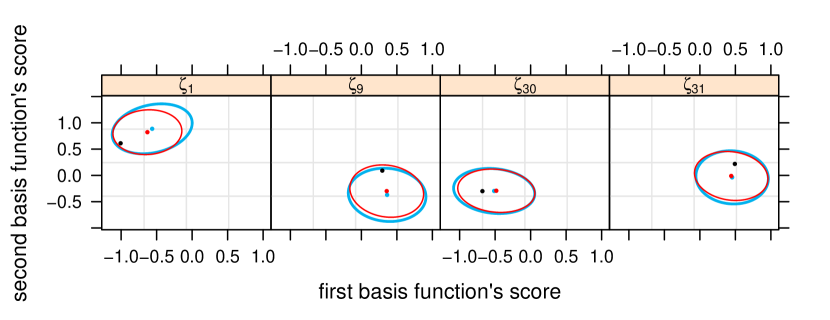
(b)

Figure 3: The results from one simulation of the Gaussian response FPCA model in (26). The simulation parameters are outlined in Section 5. In 3(a), the simulated data are shown in black, while the VMP-based variational Bayes posterior estimates are presented in red and the corresponding MCMC estimates are shown in blue. In each panel, the solid lines represent the posterior mean, while the dashed line represents the 95% pointwise credible sets for the mean. In 3(b), we present the vector of scores for each of the randomly selected response curves, shown in black, as well as the VMP-based variational Bayes posterior estimates, shown in red, and the MCMC-based posterior estimates, shown in blue. The red and blue dots represent the VMP-based variational Bayes posterior means and the MCMC-based posterior means, respectively. The ellipses represent the 95% credible contours.

5.1 Accuracy Assessment

For model (26), we simulated 36 response curves with the number of observations $T_{i}$ for the $i$th curve sampled uniformly over $\{20,21,\dots,30\}$. Furthermore, the time observations within the $i$th curve $\{t_{i1},\dots,t_{iT_{i}}\}$ were sampled uniformly over the interval $(0,1)$, while the residual variance $\sigma^{2}_{\epsilon}$ was set to 1. The mean function was

$$\mu(t)=3\sin(\pi t),$$ (55)

and the eigenfunctions were

$$\psi_{1}(t)=\sqrt{2}\sin(2\pi t)\quad\text{and}\quad\psi_{2}(t)=\sqrt{2}\cos(2\pi t),$$ (56)

Each vector of principal component scores were simulated according to

$$\bzeta_{i}=\begin{bmatrix}\zeta_{i1}\\ \zeta_{i2}\end{bmatrix}\indsim\normal\left(\begin{bmatrix}0\\ 0\end{bmatrix},\begin{bmatrix}1&0\\ 0&0.25\end{bmatrix}\right),\quad i=1,\dots,n.$$ (57)

Nonparameteric regression with O’Sullivan penalized splines for the nonlinear curves was performed with $K=10$. Finally, the simulations were conducted by setting $L=3$, rather than 2 (the number of eigenfunctions), to assess the flexibility of the VMP algorithm under slight model misspecification.

The results from the simulation are presented in Figure 3, where a random sample of four of the functional responses are selected for visual clarity. In addition, we have included the results from an MCMC treatment of model (26) in blue for comparison with the VMP-based variational Bayes fits in red. MCMC simulations were conducted through Rstan, the R r20 interface to the probabilistic programming language Stan rstan20. The variational Bayes fits have good agreement with their MCMC counterparts, as well as the simulated data. In particular, the post-VMP procedures that are outlined in Section 4 neatly complement the standard VMP algorithm.

We then incorporated five settings for the number of response curves: $n\in\{10,50,100,250,500\}$. For each of these settings, we conducted 100 simulations of model (26) with the aim of analysing the error of the posterior mean estimates of the mean curve in (55) and the functional principal component eigenfunctions in (56). The error of each simulation was determined via the integrated squared error:

$$\text{ISE}(f,\fhat)=\int_{0}^{1}\left|f(x)-\fhat(x)\right|^{2}dx,$$ (58)

where, in our simulations, $f(\cdot)$ represents the true function that generated the data, while $\fhat(\cdot)$ represents the VMP-based variational Bayes posterior mean curve.

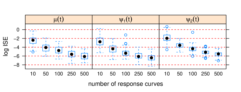
(a)

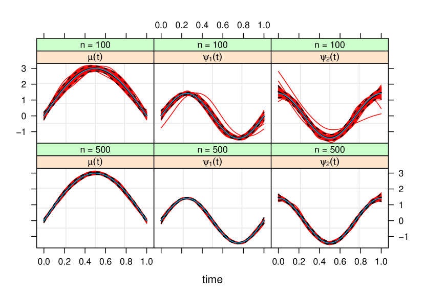
(b)

Figure 4: The results from a simulation study of the Gaussian response FPCA model in (26). The simulation parameters are outlined in Section 5.1. The box plots in 4(a) are a summary of the logarithm of the integrated squared error values in (58) for 100 simulations of each of the settings $n\in\{10,50,100,250,500\}$. In 4(b), we present the results for the mean function and the eigenfunctions when $n=100$ (top row) and $n=500$ (bottom row). The true functions are shown in blue in each panel, and the VMP-based posterior mean curve for each of the simulations is presented in red. In addition, we have included the pointwise mean curve and the pointwise 95% confidence intervals resulting from the MCMC posterior estimates for each of the generated datasets in black. Note that, in each panel, the pointwise MCMC mean curve overlaps very tightly with the true curve, making it difficult to see.

The box plots for the logarithm of the integrated squared error values in Figure 4 4(a) reflect the excellent results for the settings where $n=50,\ 100,\ 250\ \text{and}\ 500$. Overall, the results for the setting where $n=10$ are good, however, there are a few simulations where the posterior estimates of the second functional principal component eigenfunction $\psi_{2}(\cdot)$ are poor. This is to be expected because the scores associated with this eigenfunction were generated from a $\normal(0,0.25)$ distribution reflecting its weaker contribution to the data generation process. Also, as expected, the error scores for all curves tend to decline with increasing $n$. In Figure 4 4(b), we present all of the simulated posterior mean curves of the mean function and the functional principal component eigenfunctions, for the case where $n=100$ and $n=500$, which are overlaid with the true functions in blue. These plots demonstrate the strength of the VMP algorithm for estimating the underlying curves that generate an observed set of functional data. Furthermore, the variability in the curve estimates is drastically reduced with increasing $n$. In addition to each of the VMP posterior estimates, we have included the pointwise mean curve and the pointwise 95% confidence interval for the MCMC simulations for each of the generated data sets. Evidently, there is strong agreement between the VMP simulations and the MCMC simulations.

5.2 Computational Speed Comparisons

In the previous section, we saw that the mean field product restriction in (29) does not compromise the accuracy of variational Bayesian inference for FPCA. However, the major advantage offered by variational Bayesian inference via VMP is fast approximate inference in comparison to MCMC simulations. Several published articles have addressed the computational speed gains from using variational Bayesian inference. faes11 presented speed gains for parametric and nonparametric regression with missing data, luts15 presented timing comparisons for semiparametric regression models with count responses, and lee16 and nolanmw20 established speed gains for multilevel data models with streamlined matrix algebraic results. In all cases, the variational Bayesian inference algorithms had strong accuracy in comparison to MCMC simulations and were far superior in computational speed.

In Table 5.2, we present a similar set of results for the computational speed of VMP and MCMC for model (26). The simulations were identical to those that were used to generate the results in Figure 4, where there were 100 simulations over five settings for the number of response curves $n\in\{10,50,100,250,500\}$. In addition, the simulations were performed on a laptop computer with 8 GB of random access memory and a 1.6 GHz processor. In Table 5.2, we present the median elapsed computing time (in seconds), with the first quartile and the third quartile shown in brackets. Notice that most of the VMP simulations are completed within 1 minute, whereas the elapsed computing time for the MCMC simulations tends to vary from approximately 1 minute, for $n=10$, to over an hour, for $n=500$. The most impressive results are in the fourth column, where the median VMP simulation is 19.6 times faster than the median MCMC simulation for $n=10$, 34.3 times faster for $n=50$, 37.9 times faster for $n=100$, 49.0 times faster for $n=250$ and 59.8 times faster for $n=500$.

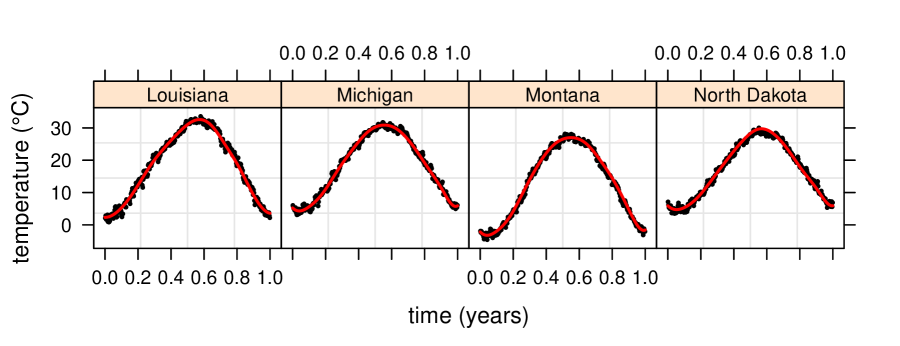
(a)

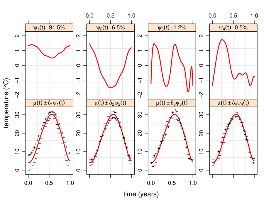
(b)

Figure 5: Application of the VMP algorithm for FPCA to the United States temperature data. The fits in 5(a) are for four randomly selected weather stations in the dataset. The plots in 5(b) present the pointwise posterior mean estimates of the eigenfunctions (top panel) and show the estimated mean function with perturbations from each eigenfunction (bottom panel): $\muhat(t)\pm\delta_{l}\psihat_{l}(t)$, $l=1,\dots,4$.

6 Application: United States Temperature Data

We now provide an illustration of our methodology with an application to temperature data collected from various United States weather stations, which is available from the rnoaa package rnoaa21 in R. The rnoaa package is an interface to the National Oceanic and Atmospheric Administration’s climate data. The function ghcnd_stations() provides access to all available global historical climatology network daily weather data for each weather site from 1960 to 1994. The information includes the longitude and latitude for each site, and this was used to determine the state or the federal district of the site. Our analysis focused on maximum daily temperature that was averaged over the 25 years of available data.

From this package, we collected full data sets (data available for every day of the year) from 2837 weather stations, where 49 states and federal districts were represented. For each state or federal district, we took a random sample of 3 of the available sites. In cases where there were less than 3 sites available (Rhode Island and District of Columbia), we used all available sites. This resulted in 145 sites used in our application, with 365 observations for each site.

Chapter 8 of ramsay05 conducts a similar analysis of Canadian temperature data from various weather stations. In their application, they uncovered four functional principal component eigenfunctions. Similarly, we conducted VMP simulations with $L=4$. The results are presented in Figure 5. In Figure 5 5(a), we display the results of four randomly selected weather stations, from four different states. There is relatively small residual variability in the observed dataset because we are using long-term averages. As a consequence, the pointwise 95% credible sets would not be visible in the plots, so we have only included the pointwise variational Bayesian posterior means. In Figure 5 5(b), we present the pointwise posterior estimates for each eigenfunction (top panel) and the the effect of perturbing the estimated mean function with each eigenfunction (bottom panel): $\muhat(t)\pm\delta_{l}\psihat_{l}(t)$, $l=1,\dots,4$. The plus (minus) signs indicate the shift that each eigenfunction makes to the mean function with a positive (negative) perturbation. In addition, the value of $\delta_{l}$ was simply selected such that the effect of the perturbation would be visibly apparent. Note that the top and bottom panels in Figure 5 5(b) should be analysed concurrently when determining the effect of each eigenfunction.

The bottom panel for the first eigenfunction (which accounts for 91.5% of the total variation) shows that it is a mean shift that perturbs the mean function in the positive (negative) direction when it is added (subtracted). The top panel shows that this effect is stronger in the Winter months than the Summer months, indicating that US temperature is most variable in Winter. Similar analysis of the second eigenfunction (which accounts for 6.5% of the total variation) shows that it represents uniformity in the measured temperatures. It perturbs the mean function in the negative (positive) direction in the Summer (Winter) months when it is added. As a consequence, weather stations at locations with larger discrepancies between Winter and Summer temperatures will have a strong and negative score for this eigenfunction. The third and fourth eigenfunctions are harder to interpret given their weak contributions to the total variation. The scores associated with the first two eigenfunctions for the displayed weather stations are (0.21, -1.26) for the weather station in Louisiana, (0.32, -0.30) for the weather station in Michigan, (-5.24, -0.04) for the weather station in Montana and (-0.66, 0.85) for the weather station in North Dakota. The scores for the first eigenfunction indicate that slightly higher than average temperatures are to be expected in Louisiana and Michigan, slightly lower than average temperatures in North Dakota and well below average temperatures in Montana. Furthermore, the scores for the second eigenfunction show that the greatest variability between Summer and Winter months can be found in Louisiana, whereas Montana may appear to be more uniform in comparison to Louisiana. In addition, Michigan experiences more than average differences in temperature between Summer and Winter, while the difference in Winter and Summer temperatures in Montana are close to the average differences in the United States.

7 Closing Remarks

We have provided a comprehensive overview of Bayesian FPCA with a VMP-based mean field variational Bayes approach. Our coverage has focused on the Gaussian likelihood specification for the observed data, and it includes the introduction of two new fragments for VMP:

1. the functional principal component Gaussian likelihood fragment (Algorithm 3.2);

2. and the functional principal component Gaussian penalization fragment (Algorithm 3.3).

These are directly compatible with the fragment-based computational constructions of VMP outlined in wand17. This is, to our knowledge, the first VMP construction of a Bayesian FPCA model. In addition, we have outlined a sequence of post-VMP steps that are necessary for producing orthonormal functional principal component eigenfunctions and uncorrelated scores.

Simulations were conducted to assess the speed and accuracy of the VMP simulations against MCMC counterparts. The approximate variational posterior density functions were in good agreement with the MCMC estimations, and the VMP algorithm was approximately 20 to 50 times faster than the MCMC algorithm depending on the number of response curves. An application to a large US temperature dataset showed that the VMP-based FPCA algorithm can be used for strong inference in big data applications.

This study could be extended to other functional data models, such as function on scalar or vector regression models, that are yet to be treated under a VMP-based mean field variational Bayes approach. In addition, extending the likelihood specification to generalized outcomes would also satisfy a popular area of research in functional data analysis.

References

• Benko \BOthers. (\APACyear2009) \APACinsertmetastarbenko09{APACrefauthors}Benko, M., Härdle, W.\BCBL \BBA Kneip, A.
Conversion to HTML had a Fatal error and exited abruptly. This document may be truncated or damaged.