Time-dependent switching of the photon entanglement type using a driven quantum emitter-cavity system

Abstract

The cascaded decay in a four-level quantum emitter is a well established mechanism to generate polarization entangled photon pairs, the building blocks of many applications in quantum technologies. The four most prominent maximally entangled photon pair states are the Bell states. In a typical experiment based on an undriven emitter only one type of Bell state entanglement can be observed in a given polarization basis. Other types of Bell state entanglement in the same basis can be created by continuously driving the system by an external laser. In this work we propose a protocol for time-dependent entanglement switching in a four-level quantum emitter–cavity system that can be operated by changing the external driving strength. By selecting different two-photon resonances between the laser-dressed states, we can actively switch back and forth between the different types of Bell state entanglement in the same basis as well as between entangled and nonentangled photon pairs. This remarkable feature demonstrates the possibility to achieve a controlled, time-dependent manipulation of the entanglement type that could be used in many innovative applications.

Entangled qubits are the building blocks for fascinating applications in many innovative research fields, like quantum cryptographyGisin et al. (2002); Lo, Curty, and Tamaki (2014), quantum communicationDuan et al. (2001); Huber et al. (2018a), or quantum information processing and computingPan et al. (2012); Bennett and DiVincenzo (2000); Kuhn et al. (2016); Zeilinger (2017). Besides possible applications, the phenomenon of entanglement is also important from a fundamental point of view, being a genuine quantum effect. Especially attractive realizations of two entangled qubits are polarization entangled photon pairs, because they travel at the speed of light and are hardly influenced by the environmentOrieux et al. (2017).

The most prominent maximally entangled states, established for polarization entangled photons pairs, are the four Bell states

$$|\Phi_{\pm}\rangle=\frac{1}{\sqrt{2}}\left(|HH\rangle\pm|VV\rangle\right),$$ (1a)

$$|\Psi_{\pm}\rangle=\frac{1}{\sqrt{2}}\left(|HV\rangle\pm|VH\rangle\right),$$ (1b)

where $H$ and $V$ denote horizontally and vertically polarized photons, respectively. The order corresponds to the order of photon detection: In a $\Phi$ Bell state ($\Phi$BS) the first and second detected photon exhibit the same polarization, whereas in a $\Psi$ Bell state ($\Psi$BS) the two detected photons have exactly the opposite polarization.

A well established mechanism for the creation of these maximally entangled Bell states is the cascaded decay that takes place in a four-level quantum emitter (FLE) after an initial excitation. Such a FLE can be realized by a variety of systems including F-centers, semiconductor quantum dots or atomsEdamatsu (2007); Freedman and Clauser (1972); Wen et al. (2008); Park et al. (2018). Employing a FLE, $\Phi$BS entanglement in the chosen basis of linearly polarized photons was demonstrated for various conditions in both theoretical and experimental studiesSeidelmann et al. (2019a); Cygorek et al. (2018); Seidelmann et al. (2019b); Schumacher et al. (2012); Heinze, Zrenner, and Schumacher (2017); Carmele and Knorr (2011); Stevenson et al. (2006); Young et al. (2006); Muller et al. (2009); Huber et al. (2018b); Wang et al. (2019); Liu et al. (2019); Bounouar et al. (2018); Dousse et al. (2010); Winik et al. (2017); Müller et al. (2014); Fognini et al. (2019); Akopian et al. (2006); Hafenbrak et al. (2007); Bennett et al. (2010); del Valle (2013); Troiani, Perea, and Tejedor (2006); Stevenson et al. (2012); Benson et al. (2000). In contrast, $\Psi$BS entanglement in the same linearly polarized basis has only been predicted in the case of continuous laser driving Sánchez Muñoz et al. (2015); Seidelmann et al. (2021). For the driven FLE laser-dressed states emerge, which have been observed experimentally Ardelt et al. (2016); Hargart et al. (2016). By embedding the FLE inside a microcavity with cavity modes tuned in resonance with the desired emission process, certain two-photon emission processes between the laser-dressed states can be favored Sánchez Muñoz et al. (2015); Seidelmann et al. (2021). The emerging type and degree of entanglement depends strongly on the dominant two-photon emission path between the laser-dressed states, which, in turn can be tuned by the external driving strength Seidelmann et al. (2021).

Based on these findings, we propose a protocol for time-dependent entanglement switching using a driven FLE-cavity system. Simply changing the external driving strength in a step-like manner enables one to actively switch between the generation of $\Phi$BS and $\Psi$BS entanglement as well as between entangled and nonentangled photon pairs. Therefore, different entangled states can be generated from the same source without further processing the photons to change the entanglement, e.g., by wave plates.

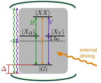
Figure 1: Sketch of the driven FLE-cavity system. The FLE consists of the states $|G\rangle$, $|X_{\text{H/V}}\rangle$, and $|XX\rangle$, which are coupled via optical transitions by horizontally/vertically polarized light (green/purple straight arrows). The FLE is driven by an external laser at the two-photon resonance which results in a detuning of $\Delta_{0}$ to the intermediate states (orange arrows). The FLE is embedded into a cavity with two energetically degenerate, but orthogonal horizontally/vertically polarized cavity modes (green/purple wavy arrows) detuned by $\Delta$ to the laser energy.

We consider an externally driven FLE-cavity system, which has been presented in detail in Refs. Sánchez Muñoz et al., 2015; Seidelmann et al., 2021. Figure 1 depicts a sketch of this system. A generic FLE comprises the ground state $|G\rangle$, two degenerate intermediate single-excited states $|X_{\text{H/V}}\rangle$, and the upper state $|XX\rangle$. Typically, $|XX\rangle$ is not found at twice the energy of the single-excited states, but is shifted by the value $E_{\text{B}}$, e.g., in quantum dots $E_{B}$ is referred to as the biexciton binding energy Orieux et al. (2017); Mermillod et al. (2016). Transitions between the FLE states that involve the state $|X_{\text{H/V}}\rangle$ are coupled to horizontally/vertically polarized light. If the $|XX\rangle$ state has been prepared Müller et al. (2014); Reiter et al. (2014); Reindl et al. (2017); Hanschke et al. (2018) cascaded photon emission takes place when the FLE relaxes to its ground state resulting in the typical $\Phi$BS.

An external laser with driving strength $\Omega$ is used to excite the FLE. The laser frequency is adjusted such that the two-photon transition between the ground state $|G\rangle$ and $|XX\rangle$ is driven resonantly, resulting in a fixed energetic detuning $\Delta_{0}=E_{\text{B}}/2$ between the single-excitation transitions and the laser (cf., Fig. 1). The laser polarization is chosen to be linear with equal components of the $H$ and $V$ polarization. The FLE is placed inside a microcavity and coupled to its two energetically degenerate linearly polarized modes, $H$ and $V$. The energetic placement of the cavity modes is described by the cavity laser detuning $\Delta$, i.e., the difference between the cavity mode and laser energy. In typical set-ups, the fabrication process determines $\Delta$ and it cannot be changed afterwards. Accordingly, we fix the cavity laser detuning to $\Delta=0.8\Delta_{0}$. The coupling strength $g$ between cavity and FLE is assumed to be equal for all FLE transitions.

Furthermore, important loss processes, i.e., radiative decay with rate $\gamma$ and cavity losses with rate $\kappa$, are included using Lindblad-type operators Seidelmann et al. (2021); Lindblad (1976). The time evolution of the statistical operator of the system and two-time correlation functions are calculated by numerically solving the resulting Liouville-von Neumann equationCosacchi et al. (2018). The system parameters for the calculations are displayed in Table 1 Sánchez Muñoz et al. (2015); Seidelmann et al. (2021). Initially the system is in the FLE ground state $|G\rangle$ without any cavity photons. For the Hamiltonian and details on the calculations we refer to Ref. Seidelmann et al., 2021.

Table 1: Fixed system parameters used in the calculations.

Parameter		Value
Coupling strength	$g$	$0.051$ meV
Detuning	$\Delta_{0}$	$20g=1.02$ meV
Cavity laser detuning	$\Delta$	$0.8\Delta_{0}=0.816$ meV
Cavity loss rate	$\kappa$	$0.1g/\hbar\approx 7.8$ $\mathrm{ns^{-1}}$
Radiative decay rate	$\gamma$	$0.01g/\hbar\approx 0.78$ $\mathrm{ns^{-1}}$

The entanglement characterization relies on the standard two-time correlation functions

$$G_{jk,lm}^{(2)}(t,\tau^{\prime})=\left\langle\hat{a}_{j}^{\dagger}(t)\hat{a}_{k}^{\dagger}(t+\tau^{\prime})\hat{a}_{m}(t+\tau^{\prime})\hat{a}_{l}(t)\right\rangle$$ (2)

with $\{j,k,l,m\}\in\{H,V\}$Cygorek et al. (2018). Here, $t$ is the real time of the first photon detection and $\tau^{\prime}$ the delay time between this detection event and the detection of the second photon. The operator $\hat{a}_{\text{H/V}}^{\dagger}$ creates one horizontally/vertically polarized cavity photonNote (1). In realistic two-time coincidence experiments the data is always obtained by averaging the signal over finite real time and delay time intervals. Consequently, we use averaged correlation functions that depend on the starting time of the coincidence measurement $t_{0}$, the used real time measurement interval $\Delta t$, and the delay time window $\tau$ (see also Ref. Seidelmann et al., 2021.).

A measure to classify the entanglement is the two-photon density matrix $\rho^{\text{2p}}$, from which the resulting type of entanglement can be extracted directly from its form. In standard experiments $\rho^{\text{2p}}$ is reconstructed employing quantum state tomographyJames et al. (2001) and, consequently, it is obtained from the averaged correlation functions as detailed in Ref. Seidelmann et al., 2021.

To quantify the degree of entanglement we use the concurrence $C$, which can be calculated directly from the two-photon density matrix Wootters (1998); del Valle (2013); James et al. (2001); Seidelmann et al. (2021); Note (2). Note that both, the two-photon density matrix and the concurrence, depend on the parameters of the coincidence measurements: $t_{0}$, $\Delta t$, and $\tau$. Throughout this article a delay time window $\tau=50$ ps is assumedStevenson et al. (2008).

Before presenting the switching protocol, we study the behavior of the constantly driven FLE-cavity system as a function of the driving strength for a fixed selected cavity laser detuning. The resulting type of entanglement and its degree depend on the cavity laser detuning $\Delta$ and the driving strength $\Omega$, as demonstrated in Ref. Seidelmann et al., 2021. In particular, a high degree of $\Phi$BS or $\Psi$BS entanglement is only possible, when the cavity modes are close to or in resonance with a direct two-photon transition between the laser-dressed states of the FLE. In the present set-up we have fixed all frequencies and detunings, such that the only free tuning parameter is the driving strength $\Omega$.

The constant driving of the FLE results in a mixing of the bare states $|G\rangle$, $|X_{\text{H/V}}\rangle$, and $|XX\rangle$, such that the new eigenstates are the laser-dressed states, which we label by $|U\rangle$, $|M\rangle$, $|N\rangle$, and $|L\rangle$. Their respective energies are given bySeidelmann et al. (2021)

$$E_{\text{U}} = \frac{1}{2}\left(\Delta_{0}+\sqrt{\Delta_{0}^{2}+8\Omega^{2}}\right)$$ (3a)

$$E_{\text{M}} = \Delta_{0}$$ (3b)

$$E_{\text{N}} = 0$$ (3c)

$$E_{\text{L}} = \frac{1}{2}\left(\Delta_{0}-\sqrt{\Delta_{0}^{2}+8\Omega^{2}}\right).$$ (3d)

Both the state mixing and the energies depend on the driving strength $\Omega$, which we will now use to tune certain two-photon transitions in resonance with the cavity modes.

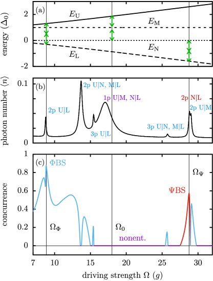
Figure 2: (a) Energies of the four laser-dressed states as function of $\Omega$ (in units of $g$). Green double-headed arrows symbolize the cavity mode energy. (b) Mean photon number $\langle n\rangle$ and (c) concurrence as functions of the driving strength $\Omega$ for a cavity laser detuning $\Delta=0.8\Delta_{0}$. $n$-photon resonances between the dressed states $|\chi_{1}\rangle$ and $|\chi_{2}\rangle$ are labeled by $n$p $\chi_{1}|\chi_{2}$. The type of entanglement is color-coded: blue = $\Phi$BS entanglement, red = $\Psi$BS entanglement, purple = no entanglement. Straight lines mark the driving strengths used for switching in Fig. 3.

Figure 2 depicts the dressed state energies [panel (a)], the mean photon number $\left\langle n\right\rangle=\langle\hat{a}_{\text{H}}^{\dagger}\hat{a}_{\text{H}}+\hat{a}_{\text{V}}^{\dagger}\hat{a}_{\text{V}}\rangle$ [panel (b)], and the concurrence [(panel (c)] as functions of the driving strength $\Omega$. All quantities are calculated at times where the system has reached its steady state, i.e., it is assumed that the coincidence measurements necessary to determine $\rho^{\text{2p}}$ and $C$ are performed after the steady state in the system dynamics has been achievedNote (3). A color code is used to distinguish between $\Phi$BS (blue) entanglement, $\Psi$BS (red) entanglement, and nonentangled photon pairs (purple).

The mean photon number exhibits a series of differently shaped peaks related to $n$-photon transitions between the four laser-dressed states. An $n$-photon transition between a pair of dressed states $|\chi_{1}\rangle$ and $|\chi_{2}\rangle$, labeled as $n$p $\chi_{1}|\chi_{2}$ in Fig. 2(b), is in resonance with the cavity modes when $n$-times the cavity laser detuning $\Delta$ matches the transition energy $E_{\chi_{1}}-E_{\chi_{2}}$. Based on this condition, all peaks of enhanced photon production can be linked to one-, two-, or three-photon resonances between the dressed states. In particular, two-photon resonances manifest themselves as high and narrow peaks, e.g., for $\Omega\approx 9g$, $14g$ or $29g$.

Turning to the concurrence, presented in Fig. 2(c), one obtains again a peak-like structure and both types of Bell state entanglement occur. By comparing the concurrences and $\left\langle n\right\rangle$, one notes that the regions of high entanglement are associated with two-photon resonances. A more detailed analysis reveals that the features observable for $\Omega\approx 14g$ ($29g$) are actually caused by two closely spaced resonances, 2p U$|$N and 2p M$|$L (2p U$|$M and 2p N$|$L), which results in a double peak in the concurrence. A particularly high degree of $\Phi$BS entanglement is obtained for $\Omega_{\Phi}=8.85g$ when the cavity mode is almost at resonance with the two-photon transition between the dressed states $|U\rangle$ and $|L\rangle$, while at $\Omega_{\Psi}=28.75g$ a high $\Psi$BS entanglement occurs at the two-photon transition between $|N\rangle$ and $|L\rangle$. This behavior can be well understood using an analysis based on a Schrieffer-Wolff transformation Seidelmann et al. (2021). Additionally, three-photon resonances lead to small peaks in the concurrence and in the mean photon number.

Besides the regions of high $\Phi$BS and $\Psi$BS entanglement, also a wide regime of vanishing concurrence is found, between $\Omega=16...25g$, where the cavity modes do not match any multi-photon transition process, cf., Fig. 2. Note that the vanishing degree of entanglement in this parameter regime is not due to a lack of emitted photons. On the contrary, the photon generation can be comparatively high due to the proximity to one-photon resonances, cf., Fig. 2(b). Therefore, in this parameter regime, the measurement detects two subsequent photons that are not entangled.

According to our findings we choose three driving strengths $\Omega_{j}$ with similar photon number, but different types of entanglement for the switching protocol: At $\Omega_{\Phi}=8.85g$ we have a strong $\Phi$BS entanglement, at $\Omega_{0}=18.00$ we have no entanglement, and at $\Omega_{\Psi}=28.75g$ we have a strong $\Psi$BS entanglement.

Figure 3: (a) The proposed protocol that enables time-dependent entanglement switching. The driving strength is changed instantaneously between the three values $\Omega_{\Phi}$, $\Omega_{\Psi}$, and $\Omega_{0}$ after a time interval $T$, resulting in a step-like time-dependent laser driving with step length $T$. During each step $j$ coincidence measurements with starting time $t_{0}$, measurement interval $\Delta t=T/4$, and delay time window $\tau=50$ ps can be performed. (b) Concurrence calculated for the respective measurements as a function of the starting time $t_{0}$ for a step length $T=1$ ns. Results are calculated for degenerate intermediate states $|X_{\text{H/V}}\rangle$ (solid line), for the finite fine-structure splitting $\delta=0.1\Delta_{0}$ between them (dashed line), and including pure dephasing with $\hbar\gamma_{\text{PD}}=3$ $\mu$eV (dotted line). The cavity laser detuning is set to $\Delta=0.8\Delta_{0}$ and the driving strength values $\Omega_{\Phi}=8.85g$, $\Omega_{\Psi}=28.75g$, and $\Omega_{0}=18g$ are used. A color code indicates $\Phi$BS (blue) and $\Psi$BS (red) entanglement as well as nonentangled photon pairs (purple). (c)-(e) Corresponding two-photon density matrices $\rho^{\text{2p}}$ obtained for the measurements performed at $t_{0}=T/2$, $3T/2$, and $5T/2$ for the case of degenerate intermediate states.

We propose a step-like excitation protocol to demonstrate time-dependent entanglement switching. The results are presented in Fig. 3. A schematic sketch of the protocol is depicted in Fig. 3(a). The basic idea is to change between three different driving strengths $\Omega_{j}$ that, in the stationary case, are associated with different types of entangled photon pairs. During the protocol, the FLE is continuously driven with a constant driving strength $\Omega_{j}$ for a fixed time period $T$ and then $\Omega$ changes step-like to one of the other two values. Accordingly, the resulting time-dependent laser driving has a step-like structure with step length $T$. In order to allow for a time resolved detection of the entanglement type, measurements with measurement interval $\Delta t=T/4$, delay time window $\tau=50$ ps, and varying starting times $t_{0}$ are performed.

Figure 3(b) displays the calculated concurrence for each measurement as a function of its respective starting time $t_{0}$, where a step length of $T=1$ ns is assumed. As before, the entanglement type is color coded: blue (red) indicates $\Phi$BS ($\Psi$BS) entanglement and purple symbolizes nonentangled photon pairs. The corresponding two-photon density matrices for the measurements performed at $t_{0}=T/2$, $3T/2$, and $5T/2$ are depicted in Fig. 3(c)-(e).

The protocol starts with driving strength $\Omega_{\Phi}$ and indeed $\Phi$BS entanglement with a high concurrence is obtained. The corresponding two-photon density matrix shown in Fig. 3(c) represents a two-photon state close to a maximally entangled $\Phi$BS. We find that the occupations of the states with two equally polarized photons, $|HH\rangle$ and $|VV\rangle$, and the coherence between them dominate $\rho^{\text{2p}}$ such that their absolute values are close to 1/2. In the second step we switch to $\Omega_{\Psi}$ and obtain a high concurrence related to $\Psi$BS entanglement. In the two-photon density matrix, presented in Fig. 3(d), the states $|HV\rangle$ and $|VH\rangle$ display the highest occupations and coherence values. In the third step with $\Omega_{0}$, the entanglement is switched off with zero concurrence. The corresponding, reconstructed density matrix is similar to a statistical mixture, where the coherences needed for an entangled Bell state are practically absent, resulting in a vanishing degree of entanglement.

Having demonstrated that all types of entanglement can be created, we continue the protocol demonstrating that the order of switching does not play a role. Accordingly, we switch in step 4 into $\Psi$BS entanglement, in step 5 we switch into $\Phi$BS entanglement and in step 6 back to no entanglement. The obtained concurrence is similar to that in step 1-3. We also checked that density matrices $\rho^{\text{2p}}$ obtained in the middle of steps 4, 5 and 6 are almost identical to those presented in Fig. 3(c)-(e) for the respective driving strength (not shown).

It is also interesting to look at the case when the measurements start in the vicinity of switching times $jT$, where $j\in\{1,2,...,5\}$. Here, one observes a continuous transition between the different entanglement types. This transition begins when the measurement starting at $t_{0}$ extends into the next step, i.e., when $t_{0}\geq jT-\Delta t$. During this transition process the degree of entanglement, as measured by the concurrence, passes through zero when one switches between $\Phi$BS and $\Psi$BS entanglement, or vice versa. After a short transition interval the measured concurrence enters either a plateau of high entanglement associated with the used driving strength or remains zero, when the driving strength is $\Omega_{0}$.

An important question is, how sensitive the proposed protocol is to parameter variations. The main requirement is that different types of entanglement can be obtained at different driving strength values. While regions of high $\Phi$BS entanglement can be found rather easily, $\Psi$BS entanglement occurs not so often. Only the two-photon transition 2p N$|$L always features $\Psi$BS entanglement, while for high driving strengths it can be found also at the 2p U$|$L resonance Seidelmann et al. (2021). Furthermore, the necessary precondition to obtain $\Psi$BS entanglement at these resonances is a finite detuning $\Delta_{0}$. In principle, in these situations, one can then switch between the different entanglement types using any finite cavity laser detuning $\Delta$. Hence we expect that the protocol also works for different values of $\Delta_{0}$ and $\Delta$. However, a more elaborate analysis suggests that high concurrence values for both entanglement types are only obtained if $\Delta$ and $\Delta_{0}$ are of the same order.

Another possible perturbation is an energy difference between the single-excited states $|X_{\text{H/V}}\rangle$, which in quantum dots is known as the fine-structure splitting (FSS). A finite FSS, defined as $\delta=\hbar\omega_{\mathrm{X_{H}}}-\hbar\omega_{\mathrm{X_{V}}}$, between the energies of the intermediate bare states $|X_{\text{H/V}}\rangle$, is regarded as a main obstacle for entanglement generation Hafenbrak et al. (2007); Bennett et al. (2010); Bounouar et al. (2018); Seidelmann et al. (2019a); Schumacher et al. (2012), because it introduces which-path information and, thus, reduces the degree of entanglementSchumacher et al. (2012); Akopian et al. (2006); Seidelmann et al. (2019a).

To consider the effect of a FSS on the switching protocol and entangled photon pair generation, we included a FSS of $\delta=0.1\Delta_{0}$ in our calculations [dashed line in Fig. 3(b)], which is a typical value being one order of magnitude smaller than the binding energyHafenbrak et al. (2007); Bounouar et al. (2018); Akopian et al. (2006); Müller et al. (2014). We find that this rather large FSS only marginally reduces the concurrence compared with the previous results. The reason is that the transitions in the driven system take place between the laser-dressed states. The FSS affects the energies of the laser-dressed states and their composition only weakly such that the resonance conditions and optical selection rules hold. This implies that the generated photonic states are practically the same and the proposed protocol is robust with respect to a non-zero FSS.

By adding a phenomenological rate modelSchumacher et al. (2012); Troiani, Perea, and Tejedor (2006)

$$\mathcal{L}_{\text{PD}}\hat{\rho}=-\frac{1}{2}\sum\limits_{\begin{subarray}{c}\chi,\chi^{\prime}\\ \chi\neq\chi^{\prime}\end{subarray}}\gamma_{\text{PD}}|\chi\rangle\langle\chi|\hat{\rho}|\chi^{\prime}\rangle\langle\chi^{\prime}|$$ (4)

with rate $\gamma_{\text{PD}}$ and $\chi,\chi^{\prime}\in\{G,X_{\text{H}},X_{\text{V}},XX\}$ acting on the statistical operator $\hat{\rho}$, we furthermore consider the influence of pure dephasing. Using a realistic value for quantum dots at low temperaturesSchumacher et al. (2012), $\hbar\gamma_{\text{PD}}=3$ $\mu$eV, we find that, although the concurrence is reduced, all essential features are unaffected. In particular, one can still switch between different entanglement types with corresponding concurrence $C\geq 0.5$ [dotted line in Fig. 3(b)].

In conclusion, this work presents a protocol for time-dependent entanglement switching based on a driven four-level emitter–cavity system. The protocol is operated by simply switching between different driving strengths in a step-like manner. Depending on the driving strength, one obtains either $\Phi$BS entanglement, $\Psi$BS entanglement or nonentangled photon pairs in the respective measurements. Thus, this work demonstrates a possibility to actively switch between different types of entanglement using a time-dependent external laser excitation. The protocol is also robust against a possible FSS. It is stressed that the protocol enables one to achieve different types of entanglement within the same basis and without further post-processing of the generated photons.

The proposed protocol is therefore a suitable candidate for the realization of time-dependent entanglement switching which is an important step towards future applications.

Data availability

The data that support the findings of this study are available from the corresponding author upon reasonable request.

References

- Gisin et al. (2002) N. Gisin, G. Ribordy, W. Tittel, and H. Zbinden, Rev. Mod. Phys. 74, 145 (2002).
- Lo, Curty, and Tamaki (2014) H.-K. Lo, M. Curty, and K. Tamaki, Nat. Photonics 8, 595 (2014).
- Duan et al. (2001) L.-M. Duan, M. D. Lukin, J. I. Cirac, and P. Zoller, Nature 414, 413 (2001).
- Huber et al. (2018a) D. Huber, M. Reindl, J. Aberl, A. Rastelli, and R. Trotta, Journal of Optics 20, 073002 (2018a).
- Pan et al. (2012) J.-W. Pan, Z.-B. Chen, C.-Y. Lu, H. Weinfurter, A. Zeilinger, and M. Żukowski, Rev. Mod. Phys. 84, 777 (2012).
- Bennett and DiVincenzo (2000) C. H. Bennett and D. P. DiVincenzo, Nature 404, 247 (2000).
- Kuhn et al. (2016) S. C. Kuhn, A. Knorr, S. Reitzenstein, and M. Richter, Opt. Express 24, 25446 (2016).
- Zeilinger (2017) A. Zeilinger, Phys. Scr. 92, 072501 (2017).
- Orieux et al. (2017) A. Orieux, M. A. M. Versteegh, K. D. Jöns, and S. Ducci, Rep. Prog. Phys. 80, 076001 (2017).
- Edamatsu (2007) K. Edamatsu, Jpn. J. Appl. Phys. 46, 7175 (2007).
- Freedman and Clauser (1972) S. J. Freedman and J. F. Clauser, Phys. Rev. Lett. 28, 938 (1972).
- Wen et al. (2008) J. Wen, S. Du, Y. Zhang, M. Xiao, and M. H. Rubin, Phys. Rev. A 77, 033816 (2008).
- Park et al. (2018) J. Park, T. Jeong, H. Kim, and H. S. Moon, Phys. Rev. Lett. 121, 263601 (2018).
- Seidelmann et al. (2019a) T. Seidelmann, F. Ungar, M. Cygorek, A. Vagov, A. M. Barth, T. Kuhn, and V. M. Axt, Phys. Rev. B 99, 245301 (2019a).
- Cygorek et al. (2018) M. Cygorek, F. Ungar, T. Seidelmann, A. M. Barth, A. Vagov, V. M. Axt, and T. Kuhn, Phys. Rev. B 98, 045303 (2018).
- Seidelmann et al. (2019b) T. Seidelmann, F. Ungar, A. M. Barth, A. Vagov, V. M. Axt, M. Cygorek, and T. Kuhn, Phys. Rev. Lett. 123, 137401 (2019b).
- Schumacher et al. (2012) S. Schumacher, J. Förstner, A. Zrenner, M. Florian, C. Gies, P. Gartner, and F. Jahnke, Opt. Express 20, 5335 (2012).
- Heinze, Zrenner, and Schumacher (2017) D. Heinze, A. Zrenner, and S. Schumacher, Phys. Rev. B 95, 245306 (2017).
- Carmele and Knorr (2011) A. Carmele and A. Knorr, Phys. Rev. B 84, 075328 (2011).
- Stevenson et al. (2006) R. M. Stevenson, R. J. Young, P. Atkinson, K. Cooper, D. A. Ritchie, and A. J. Shields, Nature 439, 179 (2006).
- Young et al. (2006) R. J. Young, R. M. Stevenson, P. Atkinson, K. Cooper, D. A. Ritchie, and A. J. Shields, New J. Phys. 8, 29 (2006).
- Muller et al. (2009) A. Muller, W. Fang, J. Lawall, and G. S. Solomon, Phys. Rev. Lett. 103, 217402 (2009).
- Huber et al. (2018b) D. Huber, M. Reindl, S. F. Covre da Silva, C. Schimpf, J. Martín-Sánchez, H. Huang, G. Piredda, J. Edlinger, A. Rastelli, and R. Trotta, Phys. Rev. Lett. 121, 033902 (2018b).
- Wang et al. (2019) H. Wang, H. Hu, T.-H. Chung, J. Qin, X. Yang, J.-P. Li, R.-Z. Liu, H.-S. Zhong, Y.-M. He, X. Ding, Y.-H. Deng, Q. Dai, Y.-H. Huo, S. Höfling, C.-Y. Lu, and J.-W. Pan, Phys. Rev. Lett. 122, 113602 (2019).
- Liu et al. (2019) J. Liu, R. Su, Y. Wei, B. Yao, S. F. C. d. Silva, Y. Yu, J. Iles-Smith, K. Srinivasan, A. Rastelli, J. Li, and X. Wang, Nat. Nanotechnol. 14, 586 (2019).
- Bounouar et al. (2018) S. Bounouar, C. de la Haye, M. Strauß, P. Schnauber, A. Thoma, M. Gschrey, J.-H. Schulze, A. Strittmatter, S. Rodt, and S. Reitzenstein, Appl. Phys. Lett. 112, 153107 (2018).
- Dousse et al. (2010) A. Dousse, J. Suffczyński, A. Beveratos, O. Krebs, A. Lemaître, I. Sagnes, J. Bloch, P. Voisin, and P. Senellart, Nature 466, 217 (2010).
- Winik et al. (2017) R. Winik, D. Cogan, Y. Don, I. Schwartz, L. Gantz, E. R. Schmidgall, N. Livneh, R. Rapaport, E. Buks, and D. Gershoni, Phys. Rev. B 95, 235435 (2017).
- Müller et al. (2014) M. Müller, S. Bounouar, K. D. Jöns, M. Glässl, and P. Michler, Nat. Photonics 8, 224 (2014).
- Fognini et al. (2019) A. Fognini, A. Ahmadi, M. Zeeshan, J. T. Fokkens, S. J. Gibson, N. Sherlekar, S. J. Daley, D. Dalacu, P. J. Poole, K. D. Jöns, V. Zwiller, and M. E. Reimer, ACS Photonics 6, 1656 (2019).
- Akopian et al. (2006) N. Akopian, N. H. Lindner, E. Poem, Y. Berlatzky, J. Avron, D. Gershoni, B. D. Gerardot, and P. M. Petroff, Phys. Rev. Lett. 96, 130501 (2006).
- Hafenbrak et al. (2007) R. Hafenbrak, S. M. Ulrich, P. Michler, L. Wang, A. Rastelli, and O. G. Schmidt, New J. Phys. 9, 315 (2007).
- Bennett et al. (2010) A. J. Bennett, M. A. Pooley, R. M. Stevenson, M. B. Ward, R. B. Patel, A. Boyer de la Giroday, N. Sköld, I. Farrer, C. A. Nicoll, D. A. Ritchie, and A. J. Shields, Nat. Phys. 6, 947 (2010).
- del Valle (2013) E. del Valle, New J. Phys. 15, 025019 (2013).
- Troiani, Perea, and Tejedor (2006) F. Troiani, J. I. Perea, and C. Tejedor, Phys. Rev. B 74, 235310 (2006).
- Stevenson et al. (2012) R. M. Stevenson, C. L. Salter, J. Nilsson, A. J. Bennett, M. B. Ward, I. Farrer, D. A. Ritchie, and A. J. Shields, Phys. Rev. Lett. 108, 040503 (2012).
- Benson et al. (2000) O. Benson, C. Santori, M. Pelton, and Y. Yamamoto, Phys. Rev. Lett. 84, 2513 (2000).
- Sánchez Muñoz et al. (2015) C. Sánchez Muñoz, F. P. Laussy, C. Tejedor, and E. del Valle, New J. Phys. 17, 123021 (2015).
- Seidelmann et al. (2021) T. Seidelmann, M. Cosacchi, M. Cygorek, D. E. Reiter, A. Vagov, and V. M. Axt, Adv. Quantum Technol. 4, 2000108 (2021).
- Ardelt et al. (2016) P.-L. Ardelt, M. Koller, T. Simmet, L. Hanschke, A. Bechtold, A. Regler, J. Wierzbowski, H. Riedl, J. J. Finley, and K. Müller, Phys. Rev. B 93, 165305 (2016).
- Hargart et al. (2016) F. Hargart, M. Müller, K. Roy-Choudhury, S. L. Portalupi, C. Schneider, S. Höfling, M. Kamp, S. Hughes, and P. Michler, Phys. Rev. B 93, 115308 (2016).
- Mermillod et al. (2016) Q. Mermillod, D. Wigger, V. Delmonte, D. E. Reiter, C. Schneider, M. Kamp, S. Höfling, W. Langbein, T. Kuhn, G. Nogues, and J. Kasprzak, Optica 3, 377 (2016).
- Reiter et al. (2014) D. E. Reiter, T. Kuhn, M. Glässl, and V. M. Axt, J. Phys.: Condens. Matter 26, 423203 (2014).
- Reindl et al. (2017) M. Reindl, K. D. Jöns, D. Huber, C. Schimpf, Y. Huo, V. Zwiller, A. Rastelli, and R. Trotta, Nano Lett. 17, 4090 (2017).
- Hanschke et al. (2018) L. Hanschke, K. A. Fischer, S. Appel, D. Lukin, J. Wierzbowski, S. Sun, R. Trivedi, J. Vucković, J. J. Finley, and K. Müller, npj Quantum Inf. 4, 43 (2018).
- Lindblad (1976) G. Lindblad, Commun. Math. Phys. 48, 119 (1976).
- Cosacchi et al. (2018) M. Cosacchi, M. Cygorek, F. Ungar, A. M. Barth, A. Vagov, and V. M. Axt, Phys. Rev. B 98, 125302 (2018).
- Note (1) Note that in typical experiments the measurements are performed on photons which have already left the cavity. Nevertheless, when the out-coupling of light out of the cavity is considered to be a Markovian process, Eq. (2\@@italiccorr) can be used to describe as measured outside of the cavity [cf. Refs. \rev@citealpnumKuhn:16,Different-Concurrences:18].
- James et al. (2001) D. F. V. James, P. G. Kwiat, W. J. Munro, and A. G. White, Phys. Rev. A 64, 052312 (2001).
- Wootters (1998) W. K. Wootters, Phys. Rev. Lett. 80, 2245 (1998).
- Note (2) where are the eigenvalues of in decreasing order and is the antidiagonal matrix with elements . .
- Stevenson et al. (2008) R. M. Stevenson, A. J. Hudson, A. J. Bennett, R. J. Young, C. A. Nicoll, D. A. Ritchie, and A. J. Shields, Phys. Rev. Lett. 101, 170501 (2008).
- Note (3) Note that in the steady state situation with constant continuous driving, and do not depend on since the statistical operator and the Hamiltonian are constant during the measurement process.