Emergence of traveling waves and their stability in a free boundary model of cell motility

Abstract

We introduce a two-dimensional Hele-Shaw type free boundary model for motility of eukaryotic cells on substrates. The key ingredients of this model are the Darcy law for overdamped motion of the cytoskeleton gel (active gel) coupled with advection-diffusion equation for myosin density leading to elliptic-parabolic Keller-Segel system. This system is supplemented with Hele-Shaw type boundary conditions: Young-Laplace equation for pressure and continuity of velocities. We first show that radially symmetric stationary solutions become unstable and bifurcate to traveling wave solutions at a critical value of the total myosin mass. Next we perform linear stability analysis of these traveling wave solutions and identify the type of bifurcation (sub- or supercritical). Our study sheds light on the mathematics underlying instability/stability transitions in this model. Specifically, we show that these transitions occur via generalized eigenvectors of the linearized operator.

1 Introduction

Motion (motility) of living cells has been the subject of extensive studies in biology, soft-matter physics and more recently in mathematics. Living cells are primarily driven by cytoskeleton gel dynamics. The study of cytoskeleton gels led to a recent development of the so-called “Active gel physics”, see [17].

The key element of this motion is cell polarity (asymmetry, e.g., the cell has a front and back), which enables cells to carry out specialized functions. Therefore understanding of cell motility and polarity are the fundamental issues in cell biology. Also, motion of specific cells such as keratocytes in the cornea is of medical relevance as they are involved, e.g., in wound healing after eye surgery or injuries. Moreover keratocytes are perfect for experiments and modeling since they are naturally found on flat surfaces, which allows capturing the main features of their motion by spatially two dimensional models. The typical modes of motion of keratocytes in cornea as well as in fishscales are rest (no movement at all) or steady motion with fixed shape, speed, and direction [13], [2]. That is why it is important to study the stationary solutions and traveling waves that describe resting cells and steadily moving cells respectively.

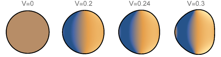
Figure 1: Approximate shape and myonsin distribution of traveling wave solutions for $m_{0}=0.62$, $R=3.6$, $\gamma=3.5$, and $k_{e}=5.0$ with $V=0,\,0.2,\,0.24,\,0.3$ bifurcated from the radial steady state. The direction of motion is to the right, and blue color corresponds to higher myosin density.

The two leading mechanisms of cell motion are protrusion generated by polymerization of actin filaments (more precisely, filamentous actin or F-actin) and contraction due to myosin motors [13]. The goal of this work is to study the contraction-driven cell motion, since it dominates motility initiation [20]. To this end we introduce and investigate a 2D model with free boundary that generalizes 1D free boundary model from [19], [20]. Despite of its simplicity this 1D model captures the bifurcation of stationary solutions to traveling waves, which is the signature property of cell motility. While mathematical analysis in 2D is obviously much more involved than in 1D, especially in the free boundary setting, the results of the bifurcation analysis in 2D agrees with 1D case [19] and [20], in particular, both models exhibit a supercritical bifurcation. However, modeling of the important phenomenon of cell shape evolution requires consideration beyond 1D and our results captures breaking of the shape symmetry, as depicted in Fig. 1, which is an important biological phenomenon, see, e.g., [2] and [25]. Moreover, the main results of this work, in particular the explicit asymptotic formula (6.10) for the eigenvalue, that decides on stability, provide a new insight for both 1D and 2D models.

Various 2D free boundary models of active gels were introduced in, e.g., [2], [6], [5]. The problems in [6] and [5] model the polymerization driven cell motion when myosin contraction is dominated by polymerization, which naturally complements present work. These models extend the classical Hele-Shaw model by adding fundamental active matter features such as the presence of persistent motion modeled by traveling wave solution. The Keller-Segel system with free boundaries as a model for contraction driven motility was first introduced in [19], in 1D setting. Its 2D counterpart introduced and analyzed numerically in [2] accounts for both polymerization and myosin contraction. A simplified version of this model was studied analytically in [4] where the traveling wave solutions were established. Note that the Keller-Segel system in fixed domains appears in various chemotaxis models and it has been extensively studied in mathematical literature due to the finite time blow-up phenomenon caused by the cross-diffusion term ([23], p.1903) in dimensions 2 and higher, see also [7] for traveling waves in the 1D flux-limited Keller-Segel model. We also mention closely related free boundary problems in tumor growth models. The key differences are that in the latter models the area of domain undergoes significant changes and there is no persistent motion (see, e.g., [9], [16], and [14]).

While in the model [2] the kinematic condition at the free boundary contains curvature, in the present work we assume continuity of velocities of the gel at the cell edge following the 1D model introduced in [19]. Still the curvature appears in the force balance on the boundary since we adapt the Young-Laplace equation for the pressure. This provides the same regularizing effect as in the classical 2D Hele-Shaw model.

The focus of this work is on understanding of transitions from unstable rest to stable motion in the model. Specifically, we establish existence of traveling wave solutions and perform their stability analysis. To show existence of a family of traveling waves we employ bifurcation analysis of the family of radially symmetric stationary solutions, following the idea originally proposed in [11] in the the framework of a tumor growth model and followed in many subsequent works on such models, e.g. [10], [12]. While aforementioned works deal with bifurcation from radial to non-radial stationary solutions via eigenvectors, in the present work we establish existence of traveling wave solutions bifurcating via generalized eigenvectors rather than eigenvectors. Similarly to [10] we use the Crandall-Rabinowitz bifurcation theorem to justify bifurcation to a family of traveling wave solutions parametrized by their velocity $V$. However, the functional framework for application of this theorem significantly differs from that is used for tumor growth models.

The main mathematical novelty of this work is in the study of spectral properties of the operator $\mathcal{A}(V)$ linearized around traveling wave solutions. The spectrum of $\mathcal{A}(V)$ near zero has rather interesting asymptotic behavior in the limit of small traveling wave velocity due to presence of non trivial Jordan chains leading to generalized eigenvectors for multiple zero eigenvalue. Specifically, $\mathcal{A}(V)$ has zero eigenvalue of multiplicity five for $V=0$ that splits into zero eigenvalue of multiplicity four and simple non zero eigenvalue $\lambda(V)\not=0$ for $V\not=0$ whose sign determines stability of traveling waves. The main result of this work is an explicit asymptotic formula (6.9) for $\lambda(V)$, which determines stability of traveling waves in terms of the total myosin mass and a special eigenvalue $E$ describing movability (see Remark 3.1) of stationary solutions.

The spectral analysis of $\mathcal{A}(V)$ has two main challenges. First, neither its coefficients nor spatial domain $\Omega(V)$ are explicitly known for $V\not=0$, since they are expressed via solution pair $\phi=\Phi(x,y,V)$, $\Omega=\Omega(V)$ of the free boundary problem (4.2)–(4.3) for traveling waves. The second principal challenge is due to non self-adjointness of the operator $\mathcal{A}(V)$, which is the signature of active matter models.

We next briefly describe main steps in the spectral analysis of $\mathcal{A}(V)$. First we assume that the perturbations have the natural symmetry of traveling wave solutions and show that at zero velocity the linearized operator $\mathcal{A}(0)$ (restricted to the space of symmetric vectors) has zero eigenvalue with multiplicity three (rather than multiplicity five in the general non-symmetric case). For $V\not=0$ the operator has zero eigenvalue of multiplicity two with an eigenvector representing infinitesimal shifts of traveling wave solutions and generalized eigenvector obtained by taking derivative of traveling wave solutions in velocity. It has also another small eigenvalue $\lambda(V)$ whose corresponding eigenvector asymptotically merges with the eigenvector representing infinitesimal shifts (this feature stands in contrast with orthogonality of eignevectors in the self-adjoint case). Moreover, finding the principlal first term in the asymptotic expansion of the eigenvalue $\lambda(V)$ requires a four term ansatz for the eigenvector, which has an interesting structure: the first two terms are the eigenvector and the generalized eigenvector of $\mathcal{A}(V)$ for the zero eigenvalue (see pairs $m_{i}$, $\rho_{i}$, $i=1,2$ in (5.9)- (5.10)). The resulting asymptotic formula (6.9) for the eigenvalue $\lambda(V)$ is remarkably simple, the principal term of $\lambda(V)$ is given in terms of two key physical quantities: movability of stationary solutions and the dependence of the total myosin mass $M(V)$ on the traveling wave velocity $V$ (see explanation after the main Theorem 7.3). However, its justification is rather involved and requires passing to the invariant subspace complementary to the generalized eigenspace of zero eigenvalue. In order to describe this invariant subspace we study generalized eigenvector of the adjoint operator that exibits singular behavior (it blows up) as $V\to 0$. Finally, we extend the results for symmetric perturbations to general perturbations of the traveling wave solutions. The key observation here is that the multiplicity of zero eigenvalue changes from two in the symmetric case to four in the general non-symmetric case. The additional eigenvector and generalized eigenvector are the infinitesimal shifts in the direction orthogonal to motion and infinitesimal rotations respectively. Thus in general case there are five eigenvalues (counted with multiplicity) of $\mathcal{A}(V)$ near zero, but only one of them is nonzero and it determines stability of traveling waves.

Acknowledgments. Volodymyr Rybalko is grateful to PSU Center for Mathematics of Living and Mimetic Matter, and to PSU Center for Interdisciplinary Mathematics for support of his two stays at Penn State. His travel was also supported by NSF grant DMS-1405769. The work L. Berlyand was partially supported by NSF grant DMS-2005262. We thank our colleagues R. Alert, I. Aronson, J. Casademunt, J.-F. Joanny, N. Meunier, A. Mogilner, J. Prost and L. Truskinovsky for useful discussions and suggestions on the model. We also express our gratitude to the members of the L. Berlyand’s PSU research team, R. Creese, M. Potomkin, and A. Safsten for careful reading and help in the preparation of the manuscript. We gratefully acknowledge numerical implementation by A. Safsten of the asymptotic expansions of traveling wave solutions established in Theorem 4.1 (Fig.1). The computational work of A. Safsten was partially supported by NSF grant DMS-2005262 and the detailed results are presented in [22].

2 The model

We consider a 2D model of motion of a cell on a flat substrate which occupies a domain $\Omega(t)$ with free boundary. The flow of the acto-myosin network inside the domain $\Omega(t)$ is described by the velocity field $u$. In the adhesion-dominated regime (overdamped flow) [6], [5] $u$ obeys the Darcy law

$$-\nabla p=\zeta u\quad\text{in}\ \Omega(t),$$ (2.1)

where $-p$ stands for the scalar stress ($p$ is the pressure) and $\zeta$ is the constant effective adhesion drag coefficient. The actomyosin network is modeled by a compressible fluid (incompressible cytoplasm fluid can be squeezed easily into the dorsal direction in the cell [15]). The main modeling assumption of this is the following constitutive law for the scalar stress $-p$

$$-p=\mu{\rm div}u+km-p_{\rm h}\quad\text{in}\ \Omega(t)$$ (2.2)

where $\mu{\rm div}u$ is the hydrodynamic stress ($\mu$ being the effective bulk viscosity of the gel), the term $km$ is the active component of the stress which is proportional to the density $m=m(x,y,t)>0$ of myosin motors with a constant contractility coefficient $k>0$, $p_{\rm h}$ is the constant hydrostatic pressure (at equilibrium). Throughout this work we assume that the effective bulk viscosity $\mu$ and the contractility coefficient $k$ in (2.2) are scaled to $\mu=1$, $k=1$. We prescribe the following condition on the boundary

$$p+p_{\rm e}=\gamma\kappa\quad\text{on}\ \partial\Omega(t),$$ (2.3)

known as the Young-Laplace equation. In (2.3) $\kappa$ denotes the curvature, $\gamma>0$ is a constant coefficient and $p_{\rm e}$ is the effective elastic restoring force which describes the mechanism of approximate conservation of the area due to the membrane-cortex tension. The elastic restoring force $p_{\rm e}$ generalizes the one-dimensional nonlocal spring condition introduced in [19], [20], see more recent work [18] which also introduces the cell volume regulating pressure, and we similarly assume the simple linear dependence of $p_{\rm e}=p_{\rm e}(|\Omega|)$ on the area:

$$p_{\rm e}=k_{\rm e}(|\Omega_{h}|-|\Omega|)/|\Omega_{h}|,$$ (2.4)

where $k_{\rm e}$ is the inverse compressibility coefficient (characterizing membrane-cortex elastic tension), $|\Omega_{h}|$ is the area of the reference configuration $\Omega_{h}$ in which $p_{e}=0$, c.f. vertex models (e.g., formula (2.2) in [1]).

The evolution of the myosin motors density is described by the advection-diffusion equation

$$\partial_{t}m=\Delta m-{\rm div}(um)\quad\text{in}\ \Omega(t)$$ (2.5)

and no flux boundary condition in the moving domain

$$\partial_{\nu}m=(u\cdot\nu-V_{\nu})m\quad\text{on}\ \partial\Omega(t),$$ (2.6)

where $\nu$ stands for the outward pointing normal vector and $V_{\nu}$ is the normal velocity of the domain $\Omega(t)$. Finally, we assume continuity of velocities on the boundary

$$V_{\nu}=u\cdot\nu,$$ (2.7)

so that (2.6) becomes the homogeneous Neumann condition. Combining (2.1)–(2.7) yields a free boundary model of the cell motility investigated in this work. While there are several models of cell motility in literature (both free boundary and phase field models), in this work we perform analytical study of stability of stationary and persistently moving states in the model (2.1)–(2.7). Moreover, the analysis of the linearized problem can be used to establish local in time existence and uniqueness of solutions.

It is convenient to introduce the potential for the velocity field $u$ using (2.1):

$$u=\nabla\phi=-\nabla\frac{1}{\zeta}p,\quad\phi:=-\frac{1}{\zeta}(p+p_{h}),$$ (2.8)

and rewrite problem (2.1)–(2.7) in the form

$$\Delta\phi+m=\zeta\phi\quad\text{in}\ \Omega(t),$$ (2.9)

$$\zeta\phi={p_{\ast}(|\Omega(t)|)}-\gamma\kappa\quad\text{on}\ \partial\Omega(t),$$ (2.10)

$$V_{\nu}=\partial_{\nu}\phi\quad\text{on}\ \partial\Omega(t),$$ (2.11)

$$\partial_{t}m=\Delta m-{\rm div}(m\nabla\phi),\quad\text{in}\ \Omega(t),$$ (2.12)

$$\partial_{\nu}m=0\quad\text{on}\ \partial\Omega(t),$$ (2.13)

where we introduced the notation

$$p_{\ast}:=p_{\rm h}+p_{\rm e}=p_{\rm h}-k_{\rm e}(|\Omega(t)|-|\Omega_{\rm h}|)/|\Omega_{\rm h}|$$ (2.14)

for the sum of the hydrostatic pressure $p_{\rm h}$ and the effective elastic restoring force $p_{\rm e}$. We assume that the area $|\Omega(t)|$ is such that (e.g., $|\Omega|$ is close to $|\Omega_{\rm h}|$)

$$p_{\ast}=p_{\ast}(|\Omega(t)|)>0.$$ (2.15)

Moreover, we consider the coefficient $k_{\rm e}$ to be sufficiently large so that it penalizes changes of the area. For instance, it prevents from shrinking of $\Omega$ to a point or from infinite expanding. The precise lower bound on $k_{\rm e}=-|\Omega_{\rm h}|\,p_{\ast}^{\prime}(|\Omega(t)|)$ is given below in (3.16).

Remark 2.1.

In this work we consider the problem (2.9)–(2.13) as an evolution problem that determines a dynamical system in the phase space of two unknowns $m(x,y,t)$ and $\Omega(t)$, while the potential $\phi(x,y,t)$ is considered as an additional unknown function defining evolution of the free boundary. Indeed, for given $\Omega(t)$ and $m(x,y,t)$ the function $\phi(x,y,t)$ is obtained as the unique solution of the elliptic problem (2.9)–(2.10), and its normal derivative $\partial_{\nu}\phi$ defines normal velocity of the boundary $\partial\Omega(t)$ due to (2.11), see also (2.7)-(2.8). Problem (2.9)–(2.13) is supplied with initial conditions for $m$ and $\Omega$ and it is natural not to include the unknown $\phi$ into the phase space of this evolution problem but rather in the definition of the operator governing the semi-group corresponding to the dynamical system in this phase space that defines the evolution of $m$ and $\Omega$ (see, e.g. (3.7)).

For technical simplicity we first assume that solutions of problem (2.9)–(2.13) is symmetric with respect to $x$-axis (it suffiices to assume such a symmetry of initial data). Subsequently we relax this assumption in Theorem 7.3 to obtain a complete characterization of linear stability of the traveling wave solutions.

3 Linear stability analysis of radially symmetric stationary solutions

In the class of radially symmetric stationary solutions with constant density $m=const$ for a given radius $R>0$ there exists the unique radial solution of the problem (2.9)–(2.13):

$$\Omega=B_{R},\quad m_{0}:=-\gamma/R+p_{\ast}(\pi R^{2}),\quad\zeta\phi_{0}={p_{\ast}(\pi R^{2})}-\gamma/R.$$ (3.1)

To describe evolution of perturbations of (3.1), it is convenient to use the polar coordinate system $(r,\varphi)$,

$$\Omega=\left\{(x=r\cos\varphi,y=r\sin\varphi);0\leq r<R+\rho(\varphi,t)\right\}.$$ (3.2)

Then linearizing problem (2.9)–(2.13) around a radially symmetric reference stationary solution (3.1), we get the following problem

$$\partial_{t}\rho=\partial_{r}\phi\quad\text{on}\ \partial B_{R},$$ (3.3)

$$\Delta\phi+m=\zeta\phi\quad\text{in}\ B_{R},$$ (3.4)

$$\phi=\frac{p_{\ast}^{\prime}(\pi R^{2})R}{\zeta}\int_{-\pi}^{\pi}\rho(\varphi)d\varphi+\frac{\gamma}{R^{2}\zeta}(\partial^{2}_{\varphi\varphi}\rho+\rho)\quad\text{on}\ \partial B_{R},$$ (3.5)

$$\partial_{t}{m}=\Delta{m}-m_{0}\Delta{\phi}\quad\text{in}\ B_{R},\quad\partial_{r}m=0\quad\text{on}\ \partial B_{R}.$$ (3.6)

This problem can be rewritten in the operator form

$$\frac{d}{dt}U=\mathcal{A}_{\rm ss}U,$$ (3.7)

where $U=(m,\rho)$, and $\mathcal{A}_{\rm ss}$ is the following operator

$$(\mathcal{A}_{\rm ss}U)_{m}=\Delta m-m_{0}\Delta\phi\quad\text{in}\ B_{R},\quad(\mathcal{A}_{\rm ss}U)_{\rho}=\partial_{r}\phi\quad\text{on}\ \partial B_{R}.$$ (3.8)

Here $\phi$ solves the time independent problem (3.4)–(3.5) for given $m$ and $\rho$. Formulas in (3.8) define an unbounded operator in $L^{2}(B_{R})\times L^{2}(\partial B_{R})$ whose domain is $H^{2}(B_{R})\cap\{m\,;\ \partial_{r}m=0\ \text{on}\ \partial B_{R}\}\times H^{3}_{\rm per}(\partial B_{R})$. Using Fourier analysis (see the proof of Theorem 3.4) one can show that this operator has a compact resolvent (alternatively, one can establish this fact following the lines of the proof of Lemma 6.5 which does not use radial symmetry).

Next we study the spectrum of the operator ${\mathcal{A}}_{\rm ss}$. Due to the radial symmetry of the problem this amounts to the Fourier analysis. Moreover we will consider only perturbations possessing the reflection symmetry with respect to the $x$-axis. That is we consider Fourier modes $m=\hat{m}(r)\cos(n\varphi)$ and $\rho=\hat{\rho}\cos(n\varphi)$ for integer $n\geq 0$. Notice that the operator ${\mathcal{A}}_{\rm ss}$ always has zero eigenvalue of multplicity at least two with eigenvectors $(m=0,\rho=\cos\varphi)$ and $(m=2\pi Rp_{\ast}^{\prime}(\pi R^{2})+\gamma/R^{2},\rho=1)$. The first of these eigenvectors represents infinitesimal shifts in the $x$-direction, and the second one is obtained by taking derivative (in $R$) of the family of stationary solutions (3.1). Next we introduce the eigenvalue $E(R)$ describing movability of stationary solutions. Namely, we will see that at the critical radius when $E(R)$ crosses zero a family of traveling wave solutions emerges.

Consider the minimization problem

$$E(R)=-\inf\left\{E_{\zeta}(m)\Bigl{/}\Bigr{.}\int_{B_{R}}m^{2}dxdy;m\in H^{1}(B_{R}),\,m=\hat{m}(r)\cos\varphi\right\},\\ \text{where}\ E_{\zeta}(m)=\int_{B_{R}}\left(|\nabla m|^{2}-m_{0}m^{2}+m_{0}\zeta|\nabla\phi|^{2}+m_{0}\zeta^{2}\phi^{2}\right)dxdy$$ (3.9)

and $\phi$ is the unique solution of the equation $\Delta\phi+m=\zeta\phi$ with the Dirichlet boundary condition $\phi=0$ on $\partial\Omega$. Minimizing the Rayleigh quotient in (3.9) yields a minimizer $m$ that satisfies $\Delta m+m_{0}m-m_{0}\zeta\phi=Em$ in $B_{R}$ and $\partial_{r}m=0$ on $\partial B_{R}$ (c.f. (3.8)). In the case when $E\not=0$ one obtains the $\rho$-component of the eigenvector by setting $\rho=\partial_{r}\phi/E$. If $E=0$, then the pair $(m,0)$ is a generalized eigenvector in the Jordan chain generated by infinitesimal shifts.

Remark 3.1.

Because of the radial symmetry, the spectral analysis of $\mathcal{A}_{ss}$ is performed via Fourier modes. The Fourier mode with $(m,\rho)=(\hat{m}(r)\cos\varphi,\hat{\rho}\cos\varphi)$ is the only mode that corresponds to motion (when the geometrical center of mass of $\Omega$ changes). There are infinitely many eigenvectors within this Fourier mode, each with a different $\hat{m}(r)$. In particular, we have the zero eigenvalue with its eigenvector corresponding to infinitesimal shifts. Then $E(R)$ is the largest of the remaining eigenvalues. That is why $E(R)$ describes movability of the stationary solutions.

Lemma 3.2.

Assume that $m_{0}\leq\zeta$, then $E(R)=0$ if and only if the solution $\Phi_{D}(r)$ of

$$\frac{1}{r}(r\Phi^{\prime}_{D}(r))^{\prime}-\frac{1}{r^{2}}\Phi_{D}(r)+(m_{0}-\zeta)\Phi_{D}(r)=m_{0}r\quad 0\leq r<R,\quad\Phi_{D}(0)=\Phi_{D}(R)=0.$$ (3.10)

satisfies the additional boundary condition

$$\Phi_{D}^{\prime}(R)=1.$$ (3.11)

Moreover, in this case $E(R)=0$ is a simple eigenvalue of the variational problem (3.9) and, up to multiplication by a constant, $m=(\Phi_{D}(r)-r)\cos\varphi$.

Proof.

Since $m=\hat{m}(r)\cos\varphi$, the solution $\phi$ of $\Delta\phi+m=\zeta\phi$ in $B_{R}$, $\phi=0$ on $\partial B_{R}$ has the representation $\phi=\hat{\phi}(r)\cos\varphi$. Now assuming that $E(R)=0$ we have $\Delta(m-m_{0}\phi)=0$, therefore $m=m_{0}(\phi-Cr\cos\varphi)$. Clearly $C\not=0$, therefore, changing the normalization if necessary, we can assume that $C=1$. Then $\phi=\Phi_{D}(r)$, and since $\partial_{r}m=0$ on $\partial B_{R}$ we obtain (3.11). Inversely, if the solution $\Phi_{D}(r)$ of (3.10) satisfies (3.11), setting $m=m_{0}(\Phi_{D}(r)-r)\cos\varphi$ we have $\phi=\Phi_{D}(r)\cos\varphi$, and

$$E(R)\geq-\frac{1}{\int_{B_{R}}m^{2}dxdy}E_{\zeta}(m)=0,\quad\text{thus}\ E(R)=0.$$

Lemma 3.2 is proved. ∎

Lemma 3.3.

Assume that $m_{0}\leq\zeta$, then $E(R)>0$, $E(R)=0$ and $E(R)<0$ if and only if $\Phi_{D}^{\prime}(R)>1$, $\Phi_{D}^{\prime}(R)=1$ and $\Phi_{D}^{\prime}(R)<1$, correspondingly, where $\Phi_{D}(r)$ is the solution of (3.10).

Proof.

Assume that $\Phi_{D}^{\prime}(R)>1$ and consider the test function $m:=m_{0}(\Phi_{D}(r)-r)\cos\varphi$. Observe that $\Delta(\Phi_{D}(r)\cos\varphi)+m=\zeta\Phi_{D}(r)\cos\varphi$, therefore we have, integrating by parts,

$$E(R)\int_{B_{R}}m^{2}dxdy\geq-E_{\zeta}(m)=-\int_{\partial B_{R}}m\partial_{r}mds+\int_{B_{R}}(\Delta m+m_{0}m-\zeta m_{0}\Phi_{D}(r)\cos\varphi)mdxdy\\ =\pi R^{2}m_{0}^{2}(\Phi_{D}^{\prime}(R)-1)>0.$$

The case $\Phi_{D}^{\prime}(R)=1$ is considered in Lemma 3.2. Finally we prove that $E(R)<0$ if $\Phi_{D}^{\prime}(R)<1$. We argue by contradiction. Assume that $E(R)>0$ and notice that allowing the parameter $\zeta$ in (3.9) increase we have a continuous function $E(R,\zeta)$ which becomes negative for sufficiently large $\zeta$. To prove the latter clame observe that otherwise there exists a sequence $\zeta_{j}\to\infty$ and $m_{j}=\hat{m}_{j}(r)\cos\varphi$ such that $\|m_{j}\|_{L^{2}(B_{R})}=1$ and $E_{\zeta_{j}}(m_{j})\leq 0$. This gives the a priori bound

$$\int_{B_{R}}|\nabla m_{j}|^{2}\,dxdy+m_{0}\zeta_{j}\int_{B_{R}}\left(|\nabla\phi_{j}|^{2}+\zeta_{j}\phi^{2}_{j}\right)\,dxdy\leq m_{0},$$ (3.12)

where $\Delta\phi_{j}+m_{j}=\zeta_{j}\phi_{j}$ in $B_{R}$, $\phi_{j}=0$ on $\partial B_{R}$. Let us show that $\zeta_{j}\phi_{j}-m_{j}\rightharpoonup 0$ weakly in $L^{2}(B_{R})$. Indeed, multiply the equation $\Delta\phi_{j}+m_{j}=\zeta_{j}\phi_{j}$ by a test function $v\in H^{1}(B_{R})$ and integrate over $B_{R}$ to get

$$\int_{B_{R}}\nabla\phi_{j}\cdot\nabla v\,dxdy+\int_{B_{R}}(\zeta_{j}\phi_{j}-m_{j})v\,dxdy=0,$$ (3.13)

and pass to the limit in this identity as $j\to\infty$. By (3.12)) we have $\|\nabla\phi_{j}\|_{L^{2}(B_{R})}<1/\sqrt{\zeta_{j}}$ therefore the second term in (3.13) tends to zero and thus the weak convergence $\zeta_{j}\phi_{j}-m_{j}\rightharpoonup 0$ is established. It follows from (3.12) that there exists $m^{\ast}\in H^{1}(B_{R})$ such that, up to a subsequence, $m_{j}\to m^{\ast}$ strongly in $L^{2}(B_{R})$, consequently

$$\liminf\limits_{j\to\infty}\|\zeta_{j}\phi_{j}\|^{2}_{L^{2}(B_{R})}-1=\liminf\limits_{j\to\infty}(\|\zeta_{j}\phi_{j}\|^{2}_{L^{2}(B_{R})}-\|m_{j}\|^{2}_{L^{2}(B_{R})})\geq 0.$$

Then (3.12) implies that $\limsup_{j\to\infty}\int_{B_{R}}|\nabla m_{j}|^{2}\,dxdy=0$, i.e. $m^{\ast}\equiv\text{const}$. On the other hand $m^{\ast}$ admits the representation $m^{\ast}=\hat{m}^{\ast}(r)\cos\varphi$. Therefore $m^{\ast}=0$ which contradicts the normalization $\|m^{\ast}\|_{L^{2}(B_{R})}=1$.

Thus, $\min E_{\hat{\zeta}}(m)/\int_{B_{R}}m^{2}dxdy=0$ for some $\tilde{\zeta}>\zeta$. Then by Lemma 3.2 the solution of

$$\frac{1}{r}(r\tilde{\Phi}^{\prime}_{D}(r))^{\prime}-\frac{1}{r^{2}}\tilde{\Phi}_{D}(r)+(m_{0}-\tilde{\zeta})\tilde{\Phi}_{D}(r)=m_{0}r\quad 0\leq r<R,\quad\tilde{\Phi}_{D}(0)=\tilde{\Phi}_{D}(R)=0.$$ (3.14)

satisfies

$$\tilde{\Phi}_{D}^{\prime}(R)=1.$$ (3.15)

But $-\frac{1}{r}(r(\tilde{\Phi}_{D}^{\prime}(r)-\Phi_{D}^{\prime}(r)))^{\prime}+\frac{1}{r^{2}}(\tilde{\Phi}_{D}(r)-\Phi_{D}(r))+(\zeta-m_{0})(\tilde{\Phi}_{D}(r)-\Phi_{D}(r))=(\zeta-\tilde{\zeta})\tilde{\Phi}_{D}>0$ for $0<r<R$, and $\tilde{\Phi}_{D}(0)-\Phi_{D}(0)=\tilde{\Phi}_{D}(R)-\Phi_{D}(R)=0$. By the maximum principle $\tilde{\Phi}_{D}(r)-\Phi_{D}(r)>0$ for $0<r<R$, therefore $\tilde{\Phi}_{D}^{\prime}(R)\leq\Phi_{D}^{\prime}(R)$, i.e. $\Phi_{D}^{\prime}(R)\geq 1$, contradiction. Lemma 3.3 is proved. ∎

The following result provides sufficient conditions for linear stability of radial stationary solutions.

Theorem 3.4.

Assume that the myosin density $m_{0}$ is bounded above by the fourth eigenvalue of the operator $-\Delta$ in $B_{R}$ with the homogeneous Neumann boundary condition on $\partial B_{R}$, also assume that $\zeta>m_{0}$ and $p_{\ast}^{\prime}(\pi R^{2})$ satisfies

$$p_{\ast}^{\prime}(\pi R^{2})<-\left(\gamma/R+2m_{0}\right)/(2\pi R^{2}).$$ (3.16)

Then $\mathcal{A}_{ss}$ has zero eigenvalue with multiplicity two if $E(R)\not=0$ or three if $E(R)=0$, and all its eigenvalues other than $0$ or $E(R)$ have negative real parts.

This theorem shows that the linear stability of stationary solutions can be described in terms of the eigenvalue $E(R)$ only. In order to determine stability/instability of the original nonlinear problem (2.9)–(2.13), an additional consideration is necessary because of the zero eigenvalue. This eigenvalue has multiplicity two; the corresponding two eigenvectors are due to the shifts and the derivative of stationary solutions (3.1) in $R$ (or equivalently in $M$). These eigenvectors generate the slow manifold formed by stationary solutions (3.1) and their shifts. While in general transition from linear to nonlinear stability in presence of zero eigenvalue may be challenging, here the conservation of total myosin mass property together with invariance with respect to shifts can be used to control the eigenvectors for the zero eigenvalue. This can be done, for instance, by generalizing the techniques from [3] developed for the tumor growth problem where authors deal with 2D slow manifold of shifts of a stationary solution.

Remark 3.5.

Due to (3.1) the total myosin mass of a radial stationary solution is $M=\pi R^{2}m_{0}=\pi R^{2}p_{\ast}(\pi R^{2})-\pi R\gamma$. Then the condition (3.16) is equivalent to

$$M^{\prime}(R)<0,$$ (3.17)

so $M(R)$ is decreasing. Notice that if $M^{\prime}(R)\not=0$ then (locally) stationary solutions can be reparametrized by $M$.

Proof.

Let $\lambda$ be an eigenvalue corresponding to an eigenvector $m=\hat{m}_{n}(r)\cos n\varphi$, $\rho=\hat{\rho}_{n}\cos n\varphi$ with $n\geq 2$. Multiply the equation $\lambda m=\Delta m+m_{0}m-m_{0}\zeta\phi$ by the complex conjugate $\overline{m}$ of $m$ and integrate over $B_{R}$,

$$\lambda\int_{B_{R}}|m|^{2}dxdy=-\int_{B_{R}}|\nabla m|^{2}dxdy+m_{0}\int_{B_{R}}|m|^{2}dxdy-m_{0}\zeta\int_{B_{R}}\phi\overline{m}dxdy.$$ (3.18)

Now multiply the equation $\overline{m}=\zeta\overline{\phi}-\Delta\overline{\phi}$ by $m_{0}\zeta\phi$ and integrate over $B_{R}$, then we obtain the following representation for the last term in (3.18):

$$m_{0}\zeta\int_{B_{R}}\phi\overline{m}dxdy=m_{0}\zeta^{2}\int_{B_{R}}|\phi|^{2}dxdy+m_{0}\zeta\int_{B_{R}}|\nabla\phi|^{2}dxdy-m_{0}\zeta\int_{\partial B_{R}}\phi{\partial_{r}\overline{\phi}}ds.$$ (3.19)

Since $\partial_{r}\overline{\phi}=\overline{\lambda}\overline{\rho}$ and (by virtue of (3.5)) $\overline{\rho}(\varphi)=\frac{R^{2}\zeta}{\gamma(1-n^{2})}\overline{\phi}(R,\varphi)$ equality (3.18) rewrites as

$$\begin{split}\lambda\int_{B_{R}}|m|^{2}dxdy+\overline{\lambda}\frac{m_{0}R^{2}\zeta^{2}}{\gamma(n^{2}-1)}\int_{\partial B_{R}}|\phi|^{2}d\sigma=&-\int_{B_{R}}|\nabla m|^{2}dxdy+m_{0}\int_{B_{R}}|m|^{2}dxdy\\ &-m_{0}\zeta\int_{B_{R}}|\nabla\phi|^{2}dxdy-m_{0}\zeta^{2}\int_{B_{R}}|\phi|^{2}dxdy.\end{split}$$ (3.20)

Notice that, thanks to the assumption that $m_{0}$ is bounded by the fourth eigenvalue of $-\Delta$ in $B_{R}$ with homogeneous Neumann boundary condition, we have

$$\int_{B_{R}}|\nabla m|^{2}dxdy-m_{0}\int_{B_{R}}|m|^{2}dxdy\geq 0.$$ (3.21)

Therefore the right hand side of (3.20) is negative, so the real part of $\lambda$ is also negative.

Next observe that all the eigenvalues whose corresponding eigenvectors have the form $m=\hat{m}(r)\cos\varphi$, $\rho=\hat{\rho}\cos\varphi$ are described by the Courant minimax principle,

$$\lambda_{j}=-\sup_{{\rm codim}S=j-1}\inf_{m\in S}\frac{E_{\zeta}(m)}{\int_{B_{R}}m^{2}dxdy},\quad\text{where $S$ is a subspace of}\ \left\{m\in H^{1}(B_{R}),\,m=\hat{m}(r)\cos\varphi\right\}.$$

Since $E_{\zeta}(m)<\int_{B_{R}}|\nabla m|^{2}dxdy-m_{0}\int_{B_{R}}m^{2}dxdy$ for $m\not=0$, the $j$-th eigenvalue $\lambda_{j}$ is bounded by the $j$-th eigenvalue of the restriction of the operator $\Delta+m_{0}$ in $B_{R}$ with the homogeneous Neumann boundary condition to the space of functions of the form $m=\hat{m}(r)\cos\varphi$. By the assumption the second eigenvalue of the latter operator is non positive, therefore $\lambda_{2}<0$ (while $\lambda_{1}=E(R)$).

Consider finally an eigenvalue $\lambda$ corresponding to a radially symmetric eigenvector. We have on $\partial B_{R}$

$$\phi=(\gamma/R^{2}+2\pi Rp_{\ast}^{\prime}(\pi R^{2}))\rho/\zeta,\quad\lambda\rho=\partial_{r}\phi=\frac{\lambda\zeta}{\gamma/R^{2}+2\pi Rp_{\ast}^{\prime}(\pi R^{2})}\phi.$$ (3.22)

Multiply the equations $\lambda m=\Delta m+m_{0}m-m_{0}\zeta\phi$ and $-\Delta\overline{\phi}+\zeta\overline{\phi}=\overline{m}$ by $\overline{m}-\langle\overline{m}\rangle$ and $\phi-\langle\phi\rangle$, where $\langle\overline{m}\rangle$, $\langle\phi\rangle$ denote mean values of $\overline{m}$, $\phi$ (over $B_{R}$), and integrate over $B_{R}$. Using integration by parts we obtain equations analogous to (3.18)-(3.19) with $m-\langle m\rangle$ and $\phi-\langle\phi\rangle$ instead of $m$ and $\phi$. Notice that

$$\int_{B_{R}}\phi(\bar{m}-\langle\bar{m}\rangle)\,dx\,dy=\int_{B_{R}}(\phi-\langle\phi\rangle)\bar{m}\,dx\,dy,$$ (3.23)

this leads to

$$\lambda\int_{B_{R}}|m-\langle{m}\rangle|^{2}dxdy= -\int_{B_{R}}|\nabla m|^{2}dxdy+m_{0}\int_{B_{R}}|m-\langle{m}\rangle|^{2}dxdy$$ (3.24)

$$-m_{0}\zeta\int_{B_{R}}\left(|\nabla\phi|^{2}+\zeta|\phi-\langle\phi\rangle|^{2}\right)dxdy+m_{0}\zeta\int_{\partial B_{R}}(\phi-\langle\phi\rangle)\partial_{r}\overline{\phi}ds.$$

Assume that $\lambda\not=0$. Then we can evaluate $\langle\phi\rangle$ in terms of $\rho$, integrating the equations $\lambda m=\Delta m+m_{0}m-m_{0}\zeta\phi$ and $-\Delta\overline{\phi}+\zeta\overline{\phi}=m$ over $B_{R}$ and eliminating $\langle m\rangle$:

$$\langle\phi\rangle=\frac{1}{\pi R^{2}\zeta}(1-m_{0}/\lambda)\int_{\partial B_{R}}\partial_{r}\phi ds=\frac{2}{R\zeta}(\lambda-m_{0})\rho.$$ (3.25)

Now we use (3.22) and (3.25) to rewrite the last term in (3.24) as

$$m_{0}\zeta\int_{\partial B_{R}}(\phi-\langle\phi\rangle)\partial_{r}\overline{\phi}ds=-4\pi m_{0}|\lambda|^{2}|\rho|^{2}+2\pi m_{0}\overline{\lambda}|\rho|^{2}\left(\gamma/R+2m_{0}+2\pi R^{2}p_{\ast}^{\prime}(\pi R^{2})\right).$$ (3.26)

Substitute (3.26) into (3.24), as the result we get

$$\lambda\int_{B_{R}} |m-\langle{m}\rangle|^{2}dxdy+4\pi m_{0}|\lambda|^{2}|\rho|^{2}-2\pi m_{0}\overline{\lambda}|\rho|^{2}\left(\gamma/R+2m_{0}+2\pi R^{2}p_{\ast}^{\prime}(\pi R^{2})\right)=$$ (3.27)

$$-\int_{B_{R}}|\nabla m|^{2}dxdy+m_{0}\int_{B_{R}}|m-\langle{m}\rangle|^{2}dxdy-m_{0}\zeta\int_{B_{R}}\left(|\nabla\phi|^{2}+\zeta|\phi-\langle\phi\rangle|^{2}\right)dxdy.$$

Thanks to the radial symmetry of $m$ the function $m-\langle{m}\rangle$ is orthogonal (with respect to the standard inner product in $L^{2}(B_{R})$) to three first eigenfunctions of the operator $\Delta$ with the homogeneous Neumann boundary condition. Therefore $\int_{B_{R}}|\nabla m|^{2}dxdy-m_{0}\int_{B_{R}}|m-\langle{m}\rangle|^{2}dxdy\geq 0$. Thus (3.27) implies that the real part of $\lambda$ is negative. To complete the proof it remains only to consider the case $\lambda=0$. There is no other eigenvector than $(m=2\pi Rp_{\ast}^{\prime}(\pi R^{2})+\gamma/R^{2},\rho=1)$ in this case, as follows from (3.24), and there is no other generalized eigenvectors, otherwise $0=\int_{B_{R}}(2\pi Rp_{\ast}^{\prime}(\pi R^{2})+\gamma/R^{2})dxdy+m_{0}\int_{\partial B_{R}}\partial_{\nu}\phi ds=\pi R(2\pi R^{2}p_{\ast}^{\prime}(\pi R^{2})+\gamma/R+2m_{0})$. Theorem 3.4 is proved. ∎

In the proof of Theorem 3.4 we have used the following simple

Proposition 3.6.

The eigenfunctions corresponding to the second and the third (if counted with multiplicity) eigenvalues of $-\Delta$ in $B_{R}$ with the homogeneous Neumann condition on $\partial B_{R}$ have the form

$$v_{2}(r,\varphi)=\hat{v}_{2}(r)\cos(\varphi+\varphi_{0})$$ (3.28)

Proof.

It suffices to show that $v_{2}(r,\varphi)$ is not a radially symmetric Fourier mode. Let $\lambda_{2}$ denote the corresponding eigenvalue. Assume by contradiction that $v_{2}(r,\varphi)=\hat{v}_{2}(r)$, then by straightforward differentiation of the eigenvalue equation one checks that $\hat{v}_{2}^{\prime}(r)\cos\varphi$ is an eigenfunction of $-\Delta$ in $B_{R}$ with the homogeneous Dirichlet condition on $\partial B_{R}$ corresponding to the eigenvalue $\lambda_{2}$. Since each eigenvalue of $-\Delta$ in $B_{R}$ with the homogeneous Dirichlet condition on $\partial B_{R}$ is strictly larger than that of $-\Delta$ in $B_{R}$ with the homogeneous Neumann condition on $\partial B_{R}$, $\lambda_{2}$ must be the first eigenvalue of the former operator. However the first eigenfunction is sign preserving, a contradiction. ∎

4 Bifurcation of traveling waves from the family of stationary solutions

In this Section we show that at the critical radius $R=R_{0}$ such that $E(R_{0})=0$ radially symmetric stationary solutions (3.1) bifurcate to a family of traveling wave solutions. It is interesting to observe that in a neighborhood of $R_{0}$ the geometric multiplicity of the zero eigenvalue of the linearized operator around stationary solutions is two as well as at $R=R_{0}$, and the bifurcation takes place via the additional generalized eigenvector appearing at $R_{0}$.

Consider the ansatz of a traveling wave solution moving with velocity $V>0$ in $x$-direction

$$m=m(x-Vt,y),\ \phi=\phi(x-Vt,y),\ \Omega(t)=\Omega+(Vt,0)$$ (4.1)

and substitute it to (2.9)–(2.13) to derive stationary free boundary problem for the unknowns $\phi$ and $\Omega$

$$\Delta\phi+\frac{M}{\int_{\Omega}e^{\phi-Vx}dxdy}e^{\phi-Vx}=\zeta\phi\quad\text{in}\ \Omega,\quad\partial_{\nu}(\phi-Vx)=0\quad\text{on}\ \partial\Omega,$$ (4.2)

$$\quad\zeta\phi=p_{\ast}(|\Omega|)-\gamma\kappa\quad\text{on}\ \partial\Omega.$$ (4.3)

Indeed, (2.12) yields $-V\partial_{x}m=\Delta m-{\rm div}(m\nabla\phi)$ in $\Omega$ while $\partial_{\nu}\phi=V\nu_{x}$ on $\partial\Omega$, then, taking into account the boundary condition $\partial_{\nu}m=0$, we see that

$$m=\Lambda e^{\phi-Vx},\quad\text{where}\ \Lambda:=\frac{M}{\int_{\Omega}e^{\phi-Vx}dxdy}.$$ (4.4)

Here unknown positive constant $M$ represents the total mass of myosin, $M=\int_{\Omega}m\,dxdy$.

For radial stationary solutions we have the following correspondence between the parameters $M$ and the radius $R$ of the domain

$$M(R)=\pi R^{2}p_{\ast}(\pi R^{2})-\pi\gamma R.$$ (4.5)

It is convenient to keep parameter $R$ in the bifurcation analysis presented below, although the domain $\Omega$ is no longer a disk. Then dependence on $R$ will appear implicitly in the parametrization of the boundary $\partial\Omega$ (as the radius of the reference disk) and explicitly in $M(R)$ given by (4.5). We use also the notation $\tilde{\Lambda}$ for the density of radial stationary solutions,

$$\tilde{\Lambda}(R):=M(R)/(\pi R^{2})=p_{\ast}(\pi R^{2})-\gamma/R,$$

reserving $m_{0}$ for the density at $R=R_{0}$.

We rely on Theorem 1.7 from [8] to get the following result on bifurcation of traveling wave solutions.

Theorem 4.1.

Let $R_{0}$ be the critical radius such that the solution of (3.10) satisfies (3.11) with $R=R_{0}$ and $m_{0}=\tilde{\Lambda}(R_{0})=p_{\ast}(\pi R_{0}^{2})-\gamma/R_{0}$. Assume also that $m_{0}<\zeta$, $m_{0}$ is bounded by the fourth eigenvalue of the $-\Delta$ in $B_{R}$ with the homogeneous Neumann boundary condition, $p_{\ast}^{\prime}(\pi R^{2}_{0})\not=-(2m_{0}-\gamma/R_{0})/(2\pi R^{2}_{0})$ and

$$F^{\prime}(R_{0})\not=0,$$ (4.6)

where

$$F(R):=\frac{\zeta I_{1}\left(R\sqrt{\zeta-\tilde{\Lambda}(R)}\right)}{(\zeta-\tilde{\Lambda}(R))^{3/2}I_{1}^{\prime}\left(R\sqrt{\zeta-\tilde{\Lambda}(R)}\right)}-\frac{R\tilde{\Lambda}(R)}{\zeta-\tilde{\Lambda}(R)},$$ (4.7)

$I_{1}$ is the 1st modified Bessel function of the first kind. Then stationary solutions (3.1) at $R=R_{0}$ bifurcate to a family of traveling wave solutions, i.e. solutions of (4.2)–(4.3) parametrized by the velocity $V$. Moreover for small $V$, $|V|\leq\overline{V}$ (for some $\overline{V}>0$), these solutions (both the function $\phi$ and the domain $\Omega$) are smooth and depend smoothly on the parameter $V$. When $V=0$ the solution of (4.2)–(4.3) is stationary and radial, $\Omega=B_{R_{0}}$, $m=\zeta\phi=m_{0}=p_{\ast}(\pi R_{0}^{2})-\gamma/R_{0}$.

Proof.

As above we consider $\Omega$ in polar coordinates, $\Omega=\{0\leq r<R+\rho(\varphi)\}$. Since $\zeta>\tilde{\Lambda}(R_{0})$, for sufficienly small $\rho$, $V$ and $R$ sufficiently close to $R_{0}$ there is a unique solution $\Phi=\Phi(x,y;V,R,\rho)$ of (4.2). It depends on three parameters: the scalar parameter $V$ (the prescribed velocity), the radius $R$ via the parametrization of the domain and $\Lambda=\Lambda(R)$, and the functional parameter $\rho$ that describes the shape of the domain $\Omega$ or, more precisely, its deviation from the disk $B_{R}$. As above we assume the symmetry of the domain with respect to the $x$-axis and therefore its shape is described by an even function $\rho$.

The condition (4.3) on the unknown boundary, described by $\rho(\varphi)$, rewrites as

$$p_{\ast}(|\Omega|)-\gamma\frac{(R+\rho)^{2}+2(\rho^{\prime})^{2}-\rho^{\prime\prime}(R+\rho)}{((R+\rho)^{2}+(\rho^{\prime})^{2})^{3/2}}=\zeta\Phi((R+\rho(\varphi))\cos\varphi,(R+\rho(\varphi))\sin\varphi,V,R,\rho).$$ (4.8)

To get rid of infinitesimal shifts we will require that

$$\int_{-\pi}^{\pi}\rho(\varphi)\cos\varphi d\varphi=0.$$ (4.9)

Then introducing the function $\mathcal{F}$ which maps from $X=C^{2}_{\rm per,even}(-\pi,\pi)\times\mathbb{R}\times\mathbb{R}$ to $Y=C^{0}_{\rm per,even}(-\pi,\pi)\times\mathbb{R}$:

$$\mathcal{F}((\rho,V),R):=\left(\gamma\frac{(R+\rho)^{2}+2(\rho^{\prime})^{2}-\rho^{\prime\prime}(R+\rho)}{\zeta((R+\rho)^{2}+(\rho^{\prime})^{2})^{3/2}}+\Phi-\frac{p_{\ast}(|\Omega|)}{\zeta},\int_{-\pi}^{\pi}\rho\cos\varphi d\varphi\right),$$ (4.10)

we rewrite problem (4.2)–(4.3) in the form

$$\mathcal{F}((\rho,V),R)=0.$$ (4.11)

Next we apply the Crandall-Rabinowitz bifurcation theorem [8] (Theorem 1.7), which guarantees bifurcation of new smooth branch of solutions provided that

• $\mathcal{F}(0,R)=0$ for all $R$ in a neighborhood of $R_{0}$;

• there exist continuous $\partial_{(\rho,V)}\mathcal{F}$, $\partial_{R}\mathcal{F}$, and $\partial^{2}_{(\rho,V),R}\mathcal{F}$ in a neighborhood of $(\rho,V)=0$, $R=R_{0}$;

• the null space $\mathrm{Null}(\partial_{(\rho,V)}\mathcal{F})$ at $(\rho,V)=0$, $R=R_{0}$ has dimension one and $\mathrm{Range}(\partial_{(\rho,V)}\mathcal{F})$ at $(\rho,V)=0$, $R=R_{0}$ has co-dimension one.

• $\partial^{2}_{(\rho,V),R}\mathcal{F}(\rho,V)\notin\mathrm{Range}(\partial_{(\rho,V)}\mathcal{F})$ at $(\rho,V)=0$, $R=R_{0}$ for all $(\rho,V)\in\mathrm{Null}(\partial_{(\rho,V)}\mathcal{F})$.

It is easy to see that condition (i) is satisfied, and condition (ii) can be verified as in [4]. To verify (iii) we begin with calculating $\mathcal{L}:=\partial_{(\rho,V)}\mathcal{F}$ at $(\rho,V)=0$. Linearizing (4.10) around $(\rho,V)=0$ we get

$$\mathcal{L}:(\rho,V)\mapsto\left(-\frac{\gamma}{R^{2}\zeta}(\rho^{\prime\prime}+\rho)+V\partial_{V}\Phi(R\cos\varphi,R\sin\varphi;0,R,0)\right.\\ \left.+\langle\partial_{\rho}\Phi,\rho\rangle\bigl{|}_{(\rho,V)=0}\bigr{.}-R\frac{p^{\prime}_{\ast}(\pi R^{2})}{\zeta}\int_{-\pi}^{\pi}\rho d\varphi,\int_{-\pi}^{\pi}\rho(\varphi)\cos\varphi d\varphi\right).$$ (4.12)

Here $\langle\partial_{\rho}\Phi,\rho\rangle\bigl{|}_{(\rho,V)=0}\bigr{.}$ denotes the Gateaux derivative of $\Phi$ at $(\rho,V)=0$. We have

$$\langle\partial_{\rho}\Phi,\rho\rangle\bigl{|}_{(\rho,V)=0}\bigr{.}=-\frac{m_{0}}{\zeta\pi R}\int_{-\pi}^{\pi}\rho\,d\varphi$$

and $\partial_{V}\Phi(R\cos\varphi,R\sin\varphi;0,R,0)=\tilde{\Phi}_{V}^{0}(R,R)\cos\varphi$, where $\tilde{\Phi}_{V}^{0}(r,R)$ solves

$$\frac{1}{r}\left(r(\tilde{\Phi}_{V}^{0})^{\prime}(r,R)\right)^{\prime}-\frac{1}{r^{2}}\tilde{\Phi}_{V}^{0}(r,R)+(\tilde{\Lambda}(R)-\zeta)\tilde{\Phi}_{V}^{0}(r,R)=\tilde{\Lambda}(R)r\quad 0\leq r<R,$$ (4.13)

$$\tilde{\Phi}_{V}^{0}(0,R)=0,\,(\tilde{\Phi}_{V}^{0})^{\prime}(r,R)\bigl{|}_{r=R}\bigr{.}=1.$$

The operator $\mathcal{L}$ has a bounded inverse when $\tilde{\Phi}_{V}^{0}(R,R)\not=0$ as can be verified by the Fourier analysis, while in the case $\tilde{\Phi}_{V}^{0}(R,R)=0$ (for $R=R_{0}$, when the operator $\mathcal{A}_{ss}$ has a generalized eigenvector corresponding to the zero eigenvalue, see Lemma 3.2) the null space of the operator $\mathcal{L}$ is one-dimensional (it is ${\rm span}\{(\rho=0,V=1)\}$) and its range consists of all the pairs $(f,C)$ such that $\int_{-\pi}^{\pi}f(\varphi)\cos\varphi d\varphi=0$. Thus, condition (iii) is satisfied.

It remains to verify the transversality condition (iv). We check if $\partial_{R}\mathcal{L}(0,1)\bigl{|}_{R=R_{0}}\bigr{.}$ does not belong to the range of the opeartor $\mathcal{L}$, where

$$\partial_{R}\mathcal{L}\bigl{|}_{R=R_{0}}:(\rho,V)\bigr{.}\mapsto\left(\frac{2\gamma}{R^{3}_{0}\zeta}(\rho^{\prime\prime}+\rho)+V\frac{d}{dR}\tilde{\Phi}_{V}^{0}\Bigl{.}\Bigr{|}_{R=R_{0}}\cos\varphi+C_{\ast}(R_{0})\int_{-\pi}^{\pi}\rho d\varphi,0\right)$$ (4.14)

with $C_{\ast}(R_{0})=-\frac{1}{\zeta}\left(p_{\ast}^{\prime}(\pi R_{0}^{2})+2\pi R_{0}^{2}p_{\ast}^{\prime\prime}(\pi R_{0}^{2})+3M/(\pi R^{2}_{0})^{2}\right)$. Since the range of $\mathcal{L}$ (described above) is all $(f,C)$ such that $f$ is orthogonal to $\cos\varphi$, we must have a nonzero coefficient in front of $\cos\varphi$ in (4.14) to satisfy condition (iv). Thus this (transversality) condition can be equivalently restated as

$$\Bigl{.}\frac{d}{dR}\tilde{\Phi}_{V}^{0}(R,R)\Bigr{|}_{R=R_{0}}\not=0.$$ (4.15)

In order to check (4.15) we change variable in (LABEL:bicond_po_drugomu) by introducing $\psi(r,R):=\tilde{\Phi}_{V}^{0}(Rr,R)$, this leads to the problem in the unit disk:

$$\frac{1}{r}(r\psi^{\prime}(r,R))^{\prime}-\frac{1}{r^{2}}\psi(r,R)+R^{2}(\tilde{\Lambda}(R)-\zeta)\psi(r,R)=R^{3}\tilde{\Lambda}(R)r\quad 0\leq r<1,$$

$$\psi(0,R)=0,\,\psi^{\prime}(r,R)\bigl{|}_{r=1}\bigr{.}=R.$$

The solution of this problem is given by

$$\psi(r,R)=-\frac{R\tilde{\Lambda}(R)}{\zeta-\tilde{\Lambda}(R)}r+\frac{\zeta I_{1}\left(R\sqrt{\zeta-\tilde{\Lambda}(R)}r\right)}{(\zeta-\tilde{\Lambda}(R))^{3/2}I_{1}^{\prime}\left(R\sqrt{\zeta-\tilde{\Lambda}(R)}\right)},$$

so that condition (4.15) writes as (4.6). ∎

Remark 4.2.

The condition (3.11) that selects the critical radius $R$ in (3.10) (which is also the necessary bifurcation condition, c.f. Theorem 3.4, item (ii)) and the transversality condition (4.6) write in terms of the function $F$ given by (4.7) as follows

$$F(R_{0})=0,\ F^{\prime}(R_{0})\not=0.$$ (4.16)

Remark 4.3.

Lemma 3.2 and comparison of the problems (LABEL:bicond_po_drugomu) and (3.10)–(3.11) show that the necessary bifurcation condition $F(R_{0})=0$ on the critical radius $R_{0}$ is satisfied iff $E(R_{0})=0$. Moreover, we show below (see (4.23)) that the second condition in (4.16) (the transversality condition) is satisfied iff $E^{\prime}(R_{0})\not=0$.

Remark 4.4.

If $\Phi=\Phi(x,y,V)$ and $\Omega(V)=\{0<r<R_{0}+\rho_{\rm tw}(\varphi,V)\}$ are the solutions of (4.2)–(4.3), then for small velocities $V$ the first term in the asymptotic expansion of the function $\rho_{\rm tw}$ is of order $V^{2}$, i.e. $\|\rho_{\rm tw}\|_{C^{2}}\leq CV^{2}$, also $\Lambda(V)=\Lambda(0)+O(V^{2})$, $\Lambda^{\prime}(0)=0$. These properties follow from Theorem 1.18 in [8]. Combining this with elliptic estimates one can improve bounds for $\rho_{\rm tw}$ to

$$\|\rho_{\rm tw}\|_{C^{j}}\leq CV^{2}\quad\forall j\in\mathbb{Z}_{+}$$ (4.17)

with $C$ depending only on $j$, and derive the following expansion for $\Phi$,

$$\Phi(x,y,V)=m_{0}/\zeta+V\Phi_{V}^{0}(x,y)+V^{2}\tilde{\Phi}(x,y,V),$$ (4.18)

where

$$\Phi_{V}^{0}=\tilde{\Phi}_{V}^{0}(r,R_{0})\cos\varphi$$ (4.19)

is the unique solution of (cf. (LABEL:bicond_po_drugomu))

$$\Delta\Phi_{V}^{0}+m_{0}(\Phi_{V}^{0}-x)=\zeta\Phi_{V}^{0}$$ (4.20)

in $B_{R}$, which satisfies

$$\Phi_{V}^{0}=0\quad\text{on}\ \partial B_{R},\quad\text{and additionally}\quad\partial_{r}\Phi_{V}^{0}=\cos\varphi\quad\text{on}\ \partial B_{R},$$ (4.21)

and functions $\tilde{\Phi}$ are uniformly (in $V$) bounded in $C^{j}(\overline{\Omega}(V))$ $\forall j\in\mathbb{Z}_{+}$. Note that $\Phi_{V}^{0}$ extends as the solution of (4.20) to the entire space $\mathbb{R}^{2}$, being a product of radially symmetric function and $\cos\varphi$.

The following lemma relates $F^{\prime}(R)$, which appears in the bifurcation condition (4.16), to $\Phi_{V}^{0}$ (the unique solution of (4.20)–(4.21)) and the derivative of the eigenvalue $E(R)$.

Lemma 4.5.

If $F(R)=0$, then the function $F^{\prime}(R)$ can be written in terms of $\Phi_{V}^{0}$ as

$$\pi\zeta RF^{\prime}(R)=\pi R(\zeta+\tilde{\Lambda}-(\tilde{\Lambda}R)^{2})-(\gamma/R^{2}+2\pi Rp_{\ast}^{\prime}(\pi R^{2}))\int_{B_{R}}|\nabla(\Phi_{V}^{0}-x)|^{2}\,dx\,dy.$$ (4.22)

Also

$$E^{\prime}(R)=-\frac{\pi\zeta RF^{\prime}(R)}{\tilde{\Lambda}\int_{B_{R}}(\Phi_{V}^{0}-x)^{2}dxdy}.$$ (4.23)

Proof.

We have $\Phi_{V}^{0}=\tilde{\Phi}_{V}^{0}(r,R)\cos\varphi$, and $\partial_{R}\tilde{\Phi}_{V}^{0}(r,R)$ satisfies the equation

$$\frac{1}{r}(r\partial_{R}(\tilde{\Phi}_{V}^{0})^{\prime})^{\prime}-\frac{1}{r^{2}}\partial_{R}\tilde{\Phi}_{V}^{0}+(\tilde{\Lambda}(R)-\zeta)\partial_{R}\tilde{\Phi}_{V}^{0}(r,R)=-\tilde{\Lambda}^{\prime}(R)(\tilde{\Phi}_{V}^{0}-r)\quad 0\leq r<R,$$ (4.24)

with boundary conditions

$$\partial_{R}\tilde{\Phi}_{V}^{0}(0,R)=0,\quad(\partial_{R}\tilde{\Phi}_{V}^{0})^{\prime}(R,R)=-(\tilde{\Phi}_{V}^{0})^{\prime\prime}(R,R)=1/R-\tilde{\Lambda}R.$$ (4.25)

Multiply (4.24) by $r\tilde{\phi}:=-r(\zeta-\tilde{\Lambda})\tilde{\Phi}_{V}^{0}-\tilde{\Lambda}r^{2}$ and integrate the result to get, using integration by parts,

$$R\left(\tilde{\Lambda}R(\tilde{\Lambda}R-1/R)+\zeta\partial_{R}\tilde{\Phi}_{V}^{0}(R,R)\right)=-\tilde{\Lambda}\tilde{\Lambda}^{\prime}\int_{0}^{R}\left(\tilde{\Phi}_{V}^{0}-r\right)^{2}rdr+\zeta\Lambda^{\prime}\int_{0}^{R}\left(\tilde{\Phi}_{V}^{0}-r\right)\tilde{\Phi}_{V}^{0}rdr,$$

or, since $\tilde{\Phi}_{V}^{0}(r,R)-r$ satisfies $\frac{1}{r}(r((\tilde{\Phi}_{V}^{0})^{\prime}-1))^{\prime}-\frac{1}{r^{2}}(\tilde{\Phi}_{V}^{0}-r)=-\tilde{\Lambda}(\tilde{\Phi}_{V}^{0}-r)+\zeta\tilde{\Phi}_{V}^{0}$ in $(0,R)$,

$$R\zeta(\partial_{R}\tilde{\Phi}_{V}^{0}(R,R)+1)=R\zeta-\tilde{\Lambda}R(\tilde{\Lambda}R^{2}-1)-\tilde{\Lambda}^{\prime}\int_{0}^{R}\left(\left((\tilde{\Phi}_{V}^{0})^{\prime}-1\right)^{2}+\left(\tilde{\Phi}_{V}^{0}(r,R)-r\right)^{2}/r^{2}\right)rdr\\ =R(\zeta+\tilde{\Lambda}-(\tilde{\Lambda}R)^{2})-\frac{\gamma/R^{2}+2\pi Rp_{\ast}^{\prime}(\pi R^{2})}{\pi}\int_{B_{R}}|\nabla(\Phi_{V}^{0}-x)|^{2}\,dx\,dy.$$

Owing to the fact that $(\tilde{\Phi}_{V}^{0})^{\prime}(R,R)=1$ the left hand side of the above relation equals $\zeta RF^{\prime}(R)$. Thus (4.22) is proved.

Now we calculate the derivative of the eigenvalue $E=E(\tilde{R})$ at $\tilde{R}=R$. Recall that $E(R)=0$ and (for $\tilde{R}$ in a small neighborhood of $R$) $E(\tilde{R})$ is a simple eigenvalue of the equation

$$Em=\Delta m+\tilde{\Lambda}(\tilde{R})m-\zeta\tilde{\Lambda}(\tilde{R})\phi(m)\quad\text{in}\ B_{\tilde{R}}$$ (4.26)

with the boundary condition $\partial_{r}m=0$ on $\partial B_{\tilde{R}}$, where $\phi(m)$ is the unique solution of the equation $\Delta\phi+m=\zeta\phi$ in $B_{\tilde{R}}$ subject to the boundary condition $\phi=0$ on $\partial B_{\tilde{R}}$. Since the problem smoothly depends on the parameter $\tilde{R}$, the eigenvalue $E(\tilde{R})$ is a smooth function of the parameter and one can choose a smooth family of eigenfunctions $m(x,y,\tilde{R})=\hat{m}(r,\tilde{R})\cos\varphi$ such that $m(x,y,R)=m_{0}(\Phi_{V}^{0}-x)$. Therefore we can differentiate (4.26) in $\tilde{R}$ to find that $\partial_{\tilde{R}}m$ at $\tilde{R}=R$ satisfies

$$E^{\prime}m=\tilde{\Lambda}^{\prime}m-\zeta\tilde{\Lambda}^{\prime}\phi(m)+\Delta\partial_{\tilde{R}}m+\tilde{\Lambda}\partial_{\tilde{R}}m-\zeta\tilde{\Lambda}\partial_{\tilde{R}}\phi(m)\quad\text{in}\ B_{R}.$$ (4.27)

Also, differentiating the equality $\partial_{r}\hat{m}(\tilde{R},\tilde{R})=0$ in $\tilde{R}$ at $\tilde{R}=R$ we find,

$$\partial_{r}\partial_{\tilde{R}}\hat{m}=-\partial^{2}_{rr}\hat{m}=-\tilde{\Lambda}\partial^{2}_{rr}\tilde{\Phi}_{V}^{0}=\frac{\tilde{\Lambda}}{R}\partial_{r}\tilde{\Phi}_{V}^{0}-\tilde{\Lambda}^{2}R=\frac{\tilde{\Lambda}}{R}-\tilde{\Lambda}^{2}R.$$ (4.28)

Now multiply (4.27) by $\Phi_{V}^{0}-x$ (the pair $\tilde{m}=\Phi_{V}^{0}-x$, $\tilde{\rho}=0$ is an element of the null space of the adjoint operator) and integrate over $B_{R}$. We have

$$E^{\prime}\tilde{\Lambda}\int_{B_{R}}(\Phi_{V}^{0}-x)^{2}dxdy =-\tilde{\Lambda}^{\prime}\int_{B_{R}}\Delta\Phi_{V}^{0}(\Phi_{V}^{0}-x)dxdy-\int_{\partial B_{R}}\partial_{r}\partial_{\tilde{R}}m\,xds$$ (4.29)

$$+\int_{B_{R}}\partial_{\tilde{R}}m\left(\Delta\Phi_{V}^{0}+\tilde{\Lambda}(\Phi_{V}^{0}-x)\right)dxdy-\zeta\tilde{\Lambda}\int_{B_{R}}\partial_{\tilde{R}}\phi(\Phi_{V}^{0}-x)dxdy.$$

Since $\Delta\Phi_{V}^{0}+\tilde{\Lambda}(\Phi_{V}^{0}-x)=\zeta\Phi_{V}^{0}$ in $B_{R}$, $\Phi_{V}^{0}=0$ on $\partial B_{R}$ and $\Delta\partial_{\tilde{R}}\phi+\partial_{\tilde{R}}m=\zeta\partial_{\tilde{R}}\phi$ in $B_{R}$, the last line in (4.29) rewrites as $\zeta\int_{\partial B_{R}}\partial_{\tilde{R}}\phi\partial_{r}\Phi_{V}^{0}\,ds$, or equivalently, $\zeta\int_{\partial B_{R}}\partial_{\tilde{R}}\phi\,x/R\,ds$. Thus

$$E^{\prime}\tilde{\Lambda}\int_{B_{R}}(\Phi_{V}^{0}-x)^{2}dxdy=\tilde{\Lambda}^{\prime}\int_{B_{R}}|\nabla(\Phi_{V}^{0}-x)|^{2}dxdy+\int_{\partial B_{R}}(\zeta\partial_{\tilde{R}}\phi/R-\partial_{r}\partial_{\tilde{R}}m)\,x\,ds.$$ (4.30)

Similarly to (4.28) one can calculate $\partial_{\tilde{R}}\phi=-\partial_{r}\Phi_{V}^{0}=-x/R$, so that $\zeta\partial_{\tilde{R}}\phi-R\partial_{r}\partial_{\tilde{R}}m=(\tilde{\Lambda}^{2}R^{2}-\zeta-\tilde{\Lambda})\cos\varphi$. Substituting this into (4.30) and calculating $\tilde{\Lambda}^{\prime}(R)=\gamma/R^{2}+2\pi Rp_{\ast}^{\prime}(\pi R^{2})$ completes the proof of Lemma 4.5. ∎

Finally, we demonstrate qualitative agreement of our analytical results with experimental results from [24]. First observe that Theorem 4.1 establishes existence of a smooth family of traveling waves in the model (2.9)–(2.13). Then one can obtain asymptotic expansions of traveling waves (solutions of (4.2)–(4.3)) in small velocities $V$, similarly to Appendix in [4]. The plots of these expansions up to $V^{3}$ show that as the velocity increases, the cell shape becomes asymmetric, with flattening of its front and the myosin accumulates at the rear. This myosin accumulation is consistent with the 1D results in [19] and [20], and the 2D results in [25] (see Fig.3 in [25]).

5 Asymptotic expansions of eigenvectors of the linearized problem

In this and the next Sections we study the spectrum of the linearized operator around traveling wave solutions, i.e. those established in Theorem 4.1. We begin with formal asymptotic expansions for small velocities $V$. These expansions will be justified in Section 6.

It is convenient to pass from the polar coordinates to the parametrization of domains via the signed distance $\rho$ from the reference domain $\Omega$. More precisely, given a solution $\phi=\Phi(x,y,V)$, $\Omega=\Omega(V)$ of problem (4.2)-(4.3), we describe perturbations $\partial\tilde{\Omega}$ of the boundary by the function $\rho$ such that $\partial\tilde{\Omega}=\{(x(s),y(s))+\rho(s)\nu(s);\ (x(s),y(s))\in\partial\Omega(V)\}$, where $s$ is the arc length parametrization of $\partial\Omega(V)$ and $\nu(s)$ denotes the outward pointing unit normal to $\partial\Omega$. Then the linearized problem around the traveling wave solution writes as

$$\Delta\phi+m=\zeta\phi\quad\text{in}\ \Omega(V),$$ (5.1)

$$\zeta(\phi+V\nu_{x}\rho)=p_{\ast}^{\prime}(|\Omega(V)|)\int_{\partial\Omega(V)}\rho(s)ds+\gamma(\rho^{\prime\prime}+\kappa^{2}\rho)\quad\text{on}\ \partial\Omega(V),$$ (5.2)

$$\partial_{t}\rho=(\mathcal{A}(V)(m,\rho))_{\rho}:=\frac{\partial\phi}{\partial\nu}+\frac{\partial^{2}\Phi}{\partial\nu^{2}}\rho-\left(\frac{\partial\Phi}{\partial\tau}+V\nu_{y}\right)\rho^{\prime}\quad\text{on}\ \partial\Omega(V),$$ (5.3)

$$\partial_{t}m=(\mathcal{A}(V)(m,\rho)))_{m}:=\Delta{m}+V\partial_{x}m-{\rm div}(\Lambda e^{\Phi-Vx}\nabla{\phi})-{\rm div}(m\nabla\Phi)\quad\text{in}\ \Omega(V),$$ (5.4)

$$\partial_{\nu}m+\Lambda e^{\Phi-Vx}\left(\frac{\partial^{2}\Phi}{\partial\nu^{2}}\rho-\Bigl{(}\frac{\partial\Phi}{\partial\tau}+V\nu_{y}\Bigr{)}\rho^{\prime}\right)=0\quad\text{on}\ \partial\Omega(V).$$ (5.5)

Here and in what follows $\rho^{\prime}$, $\rho^{\prime\prime}$ denote derivatives of $\rho$ with respect to the arc length $s$, $\kappa$ is the curvature of $\partial\Omega(V)$, and $\partial/\partial\tau$ denotes the tangential derivative on $\partial\Omega(V)$. The linearized operator $\mathcal{A}(V)$ appearing in (5.1)-(5.5) is well defined on smooth $m\in L^{2}(\Omega(V))$, $\rho\in L^{2}(\partial\Omega(V))$ such that (5.5) holds. It can be extended to the closed operator in $L^{2}(\Omega(V))\times L^{2}(\partial\Omega(V))$ whose domain is the set of pairs $(m,\rho)$ from $H^{2}(\Omega(V))\times H^{3}(\partial\Omega(V))$ satisfying (5.5).

Since traveling wave solutions bifurcate from radial stationary solutions the spectrum of the operator $\mathcal{A}(V)$ for small $|V|$ is close to the spectrum of the operator $\mathcal{A}_{ss}$ representing linearization around the radial stationary solution at the critical radius $R=R_{0}$ (heareafter we write simply $R$ for brevity). The latter oprerator has zero eigenvalue with multiplicity three while other eigenvalues are bounded away from zero. Therefore in order to study stability of traveling wave solutions it suffices to investigate what happens with zero eigenvalue for small $V\not=0$. Observe that $\forall V$ the operator $\mathcal{A}(V)$ has zero eigenvalue with multiplicity at least two. It has the eigenvector

$$m_{1}=-\Lambda(V)\partial_{x}\Phi(x,y,V),\quad\rho_{1}=\nu_{x}$$ (5.6)

corresponding to the infinitesimal shifts along the $x$-axis, and the generalized eigenvector

$$m_{2}=\partial_{V}\left(\Lambda(V)e^{\Phi(x,y,V)-Vx}\right),\quad\rho_{2}=\partial_{\tilde{V}}\tilde{\rho}\bigl{|}_{\tilde{V}=V}\bigr{.},$$ (5.7)

that satisfies $\mathcal{A}(V)(m_{2},\rho_{2})=(m_{1},\rho_{1})$, where $\tilde{\rho}$ describes the boundary of the traveling wave with velocity $\tilde{V}$ via the signed distance to $\partial\Omega(V)$. The zero eigenvalue has multiplicity three for $V=0$, as follows from Lemma (3.2). It will be shown that one eigenvalue $\lambda=\lambda(V)$ becomes nonzero for $V\not=0$ and its asymptotic behavior as $V\to 0$ is studied below. The main difficulty in this analysis comes from the fact that the eigenvector corresponding to $\lambda(V)$ merges asymptotically as $V\to 0$ with the eigenvector $(m_{1},\rho_{1})$. Moreover, the next term in the expansion of this eigenvector is proportional to $(m_{2},\rho_{2})$. That is why the asymptotic problem for $\lambda(V)$ is a kind of singularly perturbed problem.

We seek the eigenvalue $\lambda$ and the eigenvector $(m,\rho)$ in the form

$$\lambda(V)=\hat{\lambda}V^{2}+\dots,$$ (5.8)

$$m=m_{1}+\hat{\lambda}V^{2}m_{2}+V^{3}m_{3}+V^{4}m_{4}+V^{5}m_{5}+\dots$$ (5.9)

$$\rho=\rho_{1}+\hat{\lambda}V^{2}\rho_{2}+V^{3}\rho_{3}+V^{4}\rho_{4}+V^{5}\rho_{5}+\dots$$ (5.10)

with unknown $\hat{\lambda}$, $m_{k}$, $\rho_{k}$ ($k=3,4,5$) which do not depend on $V$, and will be found via perturbation expansion in $V$. In contrast, $m_{1}$, $m_{2}$, $\rho_{1}$, and $\rho_{2}$ are expressed in terms of the traveling wave solution via (5.6) and (5.7), and do depend on $V$. Observe that $\lambda(V)$ is an even function of $V$ due to the symmetry with respect to the change $V\mapsto-V$. Therefore, the ansatz (5.8) starts with a quadratic term. It is convenient to consider $\phi$ now as independent unknown, seeking this function in the form

$$\phi=-\partial_{x}\Phi+\hat{\lambda}V^{2}\partial_{V}\Phi+V^{3}\phi_{3}+V^{4}\phi_{4}+V^{5}\phi_{5}+\dots\,.$$ (5.11)

Substitute these expansions into the equation $\mathcal{A}(V)(m,\rho)=\lambda(V)(m,\rho)$ and collect terms of the order $V^{3}$, replacing $\Omega(V)$ by the disk $B_{R}$ (it approximates $\Omega(V)$ to the order $V^{2}$, see Remark 4.4). This leads to the following problem for $m_{3}$, $\phi_{3}$ and $\rho_{3}$,

$$\begin{split}&\Delta\phi_{3}+m_{3}=\zeta\phi_{3}\quad\text{in}\ B_{R},\\ &\partial_{r}\phi_{3}=0,\quad\zeta\phi_{3}=p_{\ast}^{\prime}(\pi R^{2})R\int_{-\pi}^{\pi}\rho_{3}d\varphi+\frac{\gamma}{R^{2}}(\partial^{2}_{\varphi\varphi}\rho_{3}+\rho_{3})\quad\text{on}\ \partial B_{R},\end{split}$$ (5.12)

$$\Delta m_{3}-m_{0}\Delta\phi_{3}=0\quad\text{in}\ B_{R},\quad\partial_{r}m_{3}=0\quad\text{on}\ \partial B_{R}.$$ (5.13)

Thus, up to the eigenvector corresponding to the infinitisimal shifts of the disk $B_{R}$,

$$\rho_{3}=\alpha,\ \zeta\phi_{3}=\alpha(\gamma/R^{2}+2\pi Rp_{\ast}^{\prime}(\pi R^{2})),\ m_{3}=\zeta\phi_{3}.$$ (5.14)

The parameter $\alpha$ in the solution to the homogeneous problem (5.12)–(5.13) will be determined by considering higher order terms of the expansions.

Next we collect terms of the order $V^{4}$ arriving at the following problem for $m_{4}$, $\phi_{4}$ and $\rho_{4}$,

$$\Delta\phi_{4}+m_{4}=\zeta\phi_{4}\quad\text{in}\ B_{R},$$ (5.15)

$$\Delta m_{4}-m_{0}\Delta\phi_{4}=\hat{\lambda}^{2}m_{0}(\Phi_{V}^{0}-x)+\alpha(\gamma/R^{2}+2\pi Rp_{\ast}^{\prime}(\pi R^{2}))\Delta\Phi_{V}^{0}\quad\text{in}\ B_{R},$$ (5.16)

$$\zeta\left(\phi_{4}+\alpha\partial_{r}\Phi_{V}^{0}\right)=p_{\ast}^{\prime}(\pi R^{2})R\int_{-\pi}^{\pi}\rho_{4}(\varphi)d\varphi+\frac{\gamma}{R^{2}}(\partial^{2}_{\varphi\varphi}\rho_{4}+\rho_{4})\quad\text{on}\ \partial B_{R},$$ (5.17)

$$\partial_{r}m_{4}+\alpha m_{0}\partial^{2}_{rr}\Phi_{V}^{0}=0\quad\text{on}\ \partial B_{R},$$ (5.18)

$$\frac{\partial\phi_{4}}{\partial r}+\alpha\partial^{2}_{rr}\Phi_{V}^{0}=0\quad\text{on}\ \partial B_{R}.$$ (5.19)

To determine solvability of (5.15)–(5.19) observe that after adding $\alpha m_{0}\partial_{r}\Phi_{V}^{0}$ to $m_{4}$ and $\alpha\partial_{r}\Phi_{V}^{0}$ to $\phi_{4}$, the problem is transformed to the form ${\mathcal{A}}_{ss}(m_{4}+\alpha m_{0}\partial_{r}\Phi_{V}^{0},\rho_{4})=(f(r)\cos\varphi,\varrho\cos\varphi)$ with some function $f(r)$ and a constant $\varrho$. Conditions for solvability of the latter problem are provided by the Fredholm alternative, i.e. one has to satisfy orthogonality of $(f,\varrho)$ to solutions of the adjoint homogeneous problem

$$\Delta\tilde{m}+\tilde{\phi}=0\quad\text{in}\ B_{R},\quad\partial_{r}\tilde{m}=0\quad\text{on}\ \partial B_{R},$$ (5.20)

$$\Delta\tilde{\phi}-\zeta\tilde{\phi}-m_{0}\Delta\tilde{m}=0\quad\text{in}\ B_{R},$$ (5.21)

with boundary conditions

$$\tilde{\rho}-m_{0}\tilde{m}+\tilde{\phi}=0\ \text{on}\ \partial B_{R},$$ (5.22)

$$-\frac{\gamma}{R}(\partial^{2}_{\varphi\varphi}\partial_{r}\tilde{\phi}+\partial_{r}\tilde{\phi})-\frac{R}{\zeta}p_{\ast}^{\prime}(\pi R^{2})\int_{-\pi}^{\pi}\partial_{r}\tilde{\phi}\,d\varphi=0\quad\text{on}\ \partial B_{R}.$$ (5.23)

This problem has a nontrivial solution $\tilde{m}=\Phi_{V}^{0}-x$ and $\tilde{\rho}=m_{0}\tilde{m}-\tilde{\phi}$ with $\tilde{\phi}=-(\zeta-m_{0})\Phi_{V}^{0}-m_{0}x$ (note that actually $\tilde{\rho}=0$). In order to identify the unknown coefficient $\alpha$, multiply (5.16) by $\tilde{m}$ and integrate,

$$\begin{split}\int_{B_{R}}(\Delta m_{4}-m_{0}\Delta\phi_{4})\tilde{m}dxdy&=\hat{\lambda}^{2}m_{0}\int_{B_{R}}(\Phi_{V}^{0}-x)^{2}dxdy\\ &+\alpha(\gamma/R^{2}+2\pi Rp_{\ast}^{\prime}(\pi R^{2}))\int_{B_{R}}(\Phi_{V}^{0}-x)\Delta(\Phi_{V}^{0}-x)dxdy.\end{split}$$ (5.24)

The left hand side of (5.24) rewrites as follows, using integration by parts,

$$\int_{B_{R}}(\Delta m_{4}-m_{0}\Delta\phi_{4})\tilde{m}dxdy=\int_{B_{R}}(\Delta\phi_{4}-(\zeta-m_{0})\phi_{4})\tilde{\phi}dxdy=\int_{\partial B_{R}}(\partial_{r}\phi_{4}\tilde{\phi}-\partial_{r}\tilde{\phi}\phi_{4})ds.$$ (5.25)

The functions appearing in the right hand side are $\partial_{r}\phi_{4}=\alpha(1/R-m_{0}R)\cos\varphi$, $\phi_{4}=-\alpha\cos\varphi$, $\tilde{\phi}=-m_{0}R\cos\varphi$, $\partial_{r}\tilde{\phi}=-\zeta\cos\varphi$, therefore

$$\int_{B_{R}}(\Delta m_{4}-m_{0}\Delta\phi_{4})\tilde{m}dxdy=-m_{0}\pi R^{2}\alpha(1/R-m_{0}R)-\alpha\zeta\pi R=\alpha\pi R((m_{0}R)^{2}-m_{0}-\zeta).$$ (5.26)

Thus we get the following relation between $\hat{\lambda}$ and $\alpha$,

$$\begin{split}&\alpha\left\{(-\gamma/R^{2}-2\pi Rp_{\ast}^{\prime}(\pi R^{2}))\int_{B_{R}}|\nabla(\Phi_{V}^{0}-x)|^{2}\,dx\,dy-\pi R((m_{0}R)^{2}-m_{0}-\zeta)\right\}\\ &\hskip 224.03743pt=-\hat{\lambda}^{2}m_{0}\int_{B_{R}}(\Phi_{V}^{0}-x)^{2}dxdy.\end{split}$$ (5.27)

Besides the solution $(\tilde{m}=\Phi_{V}^{0}-x,\tilde{\rho}=0)$ the problem (5.20)–(5.23) has exactly one linearly independent solution $(\tilde{m}=1,\tilde{\rho}=m_{0})$. Since $(f(r)\cos\varphi,\varrho\cos\varphi)$ is orthogonal to $(1,m_{0})$ there is a solution of (5.15)–(5.19). Moreover, if we require additionally that $m_{4}$ has zero mean value and $\rho_{4}$ is orthogonal to $\cos\varphi$ then $\rho_{4}=0$ and both $m_{4}$ and $\phi_{4}$ are represented in the form of products of radially symmetric functions and $\cos\varphi$. These radially symmetric factors solve a system of second order ordinary differential equatiuons (with bounded coefficients, except at $r=0$) and therefore extend as solutions of (5.15)–(5.16) to the whole $\mathbb{R}^{2}$. Thus the ansatz of the first four terms is well defined in $\Omega(V)$. However it is not in the domain of the operator $\mathcal{A}(V)$ as the boundary condition (5.5) is satisfied only approximately (with discrepancy of the order $O(V^{5})$). That is why we introduce a correcting term $\tilde{m}_{5}$ such that

$$\partial_{\nu}\tilde{m}_{5}=-\frac{1}{V}\partial_{\nu}m_{4}-\frac{\Lambda(V)}{V^{2}}e^{\Phi-Vx}\partial^{2}_{\nu\nu}\Phi\rho_{3}\quad\text{on}\ \partial\Omega(V).$$ (5.28)

In view of (5.18), bounds (4.17) and the expansion (4.18) (see Remark 4.4) one can show that the right hand side of (5.28) defines functions uniformly bounded in $C^{j}(\partial\Omega(V))$ $\forall j\in\mathbb{Z}_{+}$. Therefore we can define $\tilde{m}_{5}$ in $\Omega(V)$, e.g., by solving the equation $\Delta\tilde{m}_{5}=\tilde{m}_{5}$ with the boundary condition (5.28) and set

$$\tilde{W}:=(-\Lambda(V)\partial_{x}e^{\Phi-Vx},\nu_{x})+\hat{\lambda}V^{2}\partial_{\tilde{V}}(\Lambda(\tilde{V})e^{\Phi-\tilde{V}x},\tilde{\rho}_{\rm tw}(s,\tilde{V}))\bigl{|}_{\tilde{V}=V}+V^{3}(m_{3},\alpha)+V^{4}(m_{4}+V\tilde{m}_{5},0),$$ (5.29)

where $\tilde{\rho}_{\rm tw}$ stands for the parametrisation of $\partial\Omega(\tilde{V})$ via the signed distance to $\partial\Omega(V)$. The (corrected) four term ansatz given by (5.29) is in domain of the operator $\mathcal{A}(V)$ and introducing the unique solution $\tilde{\phi}_{5}$ of

$$\Delta\tilde{\phi}_{5}+\tilde{m}_{5}=\zeta\tilde{\phi}_{5}\quad\text{in}\ \Omega(V)$$

with the boundary condition

$$\zeta(\tilde{\phi}_{5}+\frac{1}{V}\phi_{4}+\frac{1}{V^{2}}\phi_{3}+\frac{\nu_{x}}{V}\rho_{3})=\frac{1}{V^{2}}\left(p_{\ast}^{\prime}(|\Omega|)\int_{\partial\Omega(V)}\rho_{3}ds+\gamma\kappa^{2}\rho_{3}\right)\quad\text{on}\ \partial\Omega(V),$$

we can calculate the components of $\mathcal{A}(V)W-\hat{\lambda}V^{2}W$:

$$\frac{1}{V^{5}}(\mathcal{A}(V)\tilde{W}-\hat{\lambda}V^{2}\tilde{W})_{m}=\Delta{\tilde{m}_{5}}+V\partial_{x}\tilde{m}_{5}-{\rm div}(\Lambda e^{\Phi-Vx}\nabla{\tilde{\phi}_{5}})-{\rm div}(\tilde{m}_{5}\nabla\Phi)\\ +\frac{1}{V}\left\{\Delta{m_{4}}+V\partial_{x}m_{4}-{\rm div}(\Lambda e^{\Phi-Vx}\nabla{\phi_{4}})-{\rm div}(m_{4}\nabla\Phi)\right\}\\ +\frac{1}{V^{2}}\left\{\Delta{m_{3}}+V\partial_{x}m_{3}-{\rm div}(\Lambda e^{\Phi-Vx}\nabla{\phi_{3}})-{\rm div}(m_{3}\nabla\Phi)\right\}\\ -\frac{\hat{\lambda}}{V}\left\{\hat{\lambda}\partial_{V}(\Lambda(V)e^{\Phi-Vx})+Vm_{3}+V^{2}m_{4}+V^{3}\tilde{m}_{5}\right\},$$ (5.30)

$$\frac{1}{V^{5}}(\mathcal{A}(V)\tilde{W}-\hat{\lambda}V^{2}\tilde{W})_{\rho}=\partial_{\nu}\tilde{\phi}_{5}+\frac{1}{V}\partial_{\nu}\phi_{4}+\frac{1}{V^{2}}\partial_{\nu}\phi_{3}+\frac{1}{V^{2}}\partial^{2}_{\nu\nu}\Phi\rho_{3}-\frac{\hat{\lambda}}{V}\left\{\hat{\lambda}\partial_{\tilde{V}}\tilde{\rho}_{\rm tw}\bigl{|}_{\tilde{V}=V}\bigr{.}+V\rho_{3}\right\}.$$ (5.31)

Thanks to (5.12), (5.17) we have $\|\tilde{\phi}_{5}\|_{C^{j}(\partial\Omega(V))}\leq C_{j}$ $\forall j\in\mathbb{Z}_{+}$, also one can verify that normal derivatives $\partial_{\nu}\tilde{\phi}$ are uniformly bounded in $C^{j}(\partial\Omega(V))$ $\forall j\in\mathbb{Z}_{+}$, similarly to $\partial_{\nu}\tilde{m}_{5}$. Furthermore, since $m_{3}$, $\phi_{3}$ are constants the third line of (5.30) simplifies to $-m_{3}\Delta\Phi/V^{2}$ and substituting $\Delta m_{4}$ from (5.16) we obtain after rearranging terms,

$$\frac{1}{V^{5}}(\mathcal{A}(V)\tilde{W}-\hat{\lambda}V^{2}\tilde{W})_{m}=\Delta{\tilde{m}_{5}}+V\partial_{x}\tilde{m}_{5}-{\rm div}(\Lambda e^{\Phi-Vx}\nabla{\tilde{\phi}_{5}})-{\rm div}(\tilde{m}_{5}\nabla\Phi)$$ (5.32)

$$-\frac{\hat{\lambda}^{2}}{V}\left\{\partial_{V}(\Lambda(V)e^{\Phi-Vx})-m_{0}(\Phi_{V}^{0}-x)\right\}$$

$$+\frac{1}{V}\left\{V\partial_{x}m_{4}-{\rm div}((\Lambda e^{\Phi-Vx}-m_{0})\nabla{\phi_{4}})-{\rm div}(m_{4}\nabla\Phi)\right\}$$

$$-\hat{\lambda}(m_{3}+Vm_{4}+V^{2}\tilde{m}_{5})+\frac{m_{3}}{V^{2}}(V\Delta\Phi_{V}^{0}-\Delta\Phi)$$

$$\frac{1}{V^{5}}(\mathcal{A}(V)\tilde{W}-\hat{\lambda}V^{2}\tilde{W})_{\rho}=\partial_{\nu}\tilde{\phi}_{5}+\frac{1}{V}\partial_{\nu}\phi_{4}+\frac{1}{V^{2}}\partial^{2}_{\nu\nu}\Phi\rho_{3}-\frac{\hat{\lambda}}{V}(\hat{\lambda}\partial_{V}\tilde{\rho}_{\rm tw}+V\rho_{3}).$$ (5.33)

Thus $\|(\mathcal{A}(V)\tilde{W}-\hat{\lambda}V^{2}\tilde{W})_{m}\|_{L^{2}(\Omega(V))}+\|(\mathcal{A}(V)\tilde{W}-\hat{\lambda}V^{2}\tilde{W})_{\rho}\|_{L^{2}(\partial\Omega(V))}\leq C|V|^{5}$.

Next assuming that there exists the next term $V^{5}(m_{5},\rho_{5})$ of the asymptotic expansion, we have, neglecting higher order terms, $\mathcal{A}(V)(m_{5},\rho_{5})=-\frac{1}{V^{5}}(\mathcal{A}(V)W-\hat{\lambda}V^{2}W)$. Since the null space of the adjoint operator $\mathcal{A}^{\ast}(V)$ contains $(1,\Lambda(V)e^{\Phi-Vx})$ (see (5.51)), we will require that

$$\int_{\Omega(V)}(\mathcal{A}(V)\tilde{W}-\hat{\lambda}V^{2}\tilde{W})_{m}\,dxdy+\Lambda(V)\int_{\partial\Omega(V)}(\mathcal{A}(V)\tilde{W}-\hat{\lambda}V^{2}\tilde{W})_{\rho}e^{\Phi-Vx}\,ds=0.$$ (5.34)

We will see that this condition yields an asymptotic formula for $\hat{\lambda}$.

Let $I(\hat{\lambda},V)$ denote the left hand side of (5.34), then with the help of integration by parts and (5.28), (5.33) we get

$$I(\hat{\lambda}) =\frac{1}{V}\int_{\partial\Omega(V)}(\Lambda(V)e^{\Phi-Vx}\partial_{\nu}\phi_{4}-\partial_{\nu}m_{4})\,ds-\int_{\partial\Omega(V)}\hat{\lambda}\rho_{3}\Lambda(V)e^{\Phi-Vx}\,ds$$ (5.35)

$$+\int_{\Omega(V)}\left(V\partial_{x}\tilde{m}_{5}-{\rm div}(\tilde{m}_{5}\nabla\Phi)\right)\,dxdy+\frac{1}{V}\int_{\Omega(V)}(\hat{\lambda}^{2}m_{0}(\Phi_{V}^{0}-x)+m_{3}\Delta\Phi_{V}^{0})\,dxdy$$

$$+\frac{1}{V}\int_{\Omega(V)}\left\{V\partial_{x}m_{4}-{\rm div}((\Lambda e^{\Phi-Vx}-m_{0})\nabla{\phi_{4}})-{\rm div}(m_{4}\nabla\Phi)\right\}\,dxdy$$

$$-\hat{\lambda}\int_{\Omega(V)}(m_{3}+Vm_{4}+V^{2}\tilde{m}_{5})\,dxdy$$

$$-\frac{\hat{\lambda}^{2}}{V}\left\{\int_{\partial\Omega(V)}\partial_{V}(\Lambda(V)e^{\Phi-Vx})\,ds+\int_{\partial\Omega(V)}\Lambda(V)e^{\Phi-Vx}\partial_{V}\tilde{\rho}_{\rm tw}\,ds\right\}.$$

This formula is further simplified by observing that the first term in the second line of (5.35) is zero thanks to the fact that $\partial_{\nu}\Phi=\nu_{x}$ on $\partial\Omega(V)$. Also, using (5.16) in the second term, then collecting all the terms with the prefactor $\frac{1}{V}$ except the last line, we see that these terms cancel each other. Finally, notice that the last line of (5.35) equals $-\frac{\hat{\lambda}^{2}}{V}M^{\prime}(V)$. Thus

$$I(\hat{\lambda},V)=-\hat{\lambda}\alpha\pi R(2m_{0}+\gamma/R+2\pi R^{2}p^{\prime}_{\ast}(\pi R^{2})+O(V))-\frac{\hat{\lambda}^{2}}{V}M^{\prime}(V),$$ (5.36)

and substituting $\alpha$ from (5.27) we see that the equation $I(\hat{\lambda},V)=0$ has nonzero solution

$$\hat{\lambda}(V)=-\frac{(\gamma/R^{2}+2\pi Rp_{\ast}^{\prime}(\pi R^{2}))\int_{B_{R}}|\nabla(\Phi_{V}^{0}-x)|^{2}\,dxdy+\pi R((m_{0}R)^{2}-m_{0}-\zeta)}{\pi m_{0}R(2m_{0}+\gamma/R+2\pi R^{2}p_{\ast}^{\prime}(\pi R^{2})+O(V))\int_{B_{R}}(\Phi_{V}^{0}-x)^{2}\,dxdy}\frac{M^{\prime}(V)}{V}$$ (5.37)

for sufficiently small $V$, provided that $M^{\prime}(V)\not=0$ when $V\not=0$. The first factor in (5.37) simplifies, by virtue of (4.22)–(4.23), to $-\frac{dE}{dM}\bigl{|}_{M=M_{0}}\bigr{.}$, where $M_{0}$ is the total myosin mass of the stationary solution (with $V=0$). In the nondegenerate case, $M^{\prime\prime}(0)\not=0$, the solution $\hat{\lambda}(V)$ has nonzero finite limit

$$\hat{\lambda}=-\frac{dE}{dM}\Bigl{|}_{M=M_{0}}\Bigr{.}\frac{d^{2}M}{dV^{2}}\Bigl{|}_{V=0}\Bigr{.}.$$ (5.38)

If $M^{\prime\prime}(0)=0$ but $M^{\prime}(V)\not=0$ for small $V\not=0$ there still exists a nonzero solution $\hat{\lambda}(V)$ of the equation $I(\hat{\lambda},V)=0$ and we can repeat the above construction observing that in this case $m_{3}$, $\rho_{3}$, $m_{4}$ and $\tilde{m}_{5}$ contain the small factor $\alpha=O\left((M^{\prime}(V)/V)^{2}\right)$.

We summarize the results of the above asymptotic analysis in the following lemma that provides the construction of the approximation for the eigenvalue $\lambda(V)$ and the corresponding eigenvector. It also plays an important role in the justification of the asymptotic formula for the eigenvalue $\lambda(V)$ in Section 6.

Lemma 5.1.

Assume that $M^{\prime}(V)\not=0$ for small $V\not=0$, then there exists $\hat{\lambda}(V)$ and $\tilde{W}=(\tilde{m},\tilde{\rho})$ in the domain of $\mathcal{A}(V)$ such that

$$\tilde{W}=(-\Lambda(V)\partial_{x}e^{\Phi-Vx},\nu_{x})+O(V^{2}),$$ (5.39)

$$\|(\mathcal{A}(V)\tilde{W}-\hat{\lambda}(V)V^{2}\tilde{W})_{m}\|_{L^{2}(\Omega(V))}+\|(\mathcal{A}(V)\tilde{W}-\hat{\lambda}V^{2}\tilde{W})_{\rho}\|_{L^{2}(\partial\Omega(V))}\leq C|M^{\prime}(V)|^{2}|V|^{3}$$ (5.40)

and

$$\langle\mathcal{A}(V)\tilde{W}-\hat{\lambda}(V)V^{2}\tilde{W},W_{1}^{\ast}\rangle_{L^{2}}=0,$$ (5.41)

where $\langle\,\cdot\,,\,\cdot\,\rangle_{L^{2}}$ denotes the pairing defined by (5.44), and $W_{1}^{\ast}=(1,\Lambda(V)e^{\Phi-Vx})$. Moreover, $\hat{\lambda}(V)\not=0$ for $V\not=0$ and is given by the asymptotic formula

$$\hat{\lambda}(V)=-\frac{dE}{dM}\Bigl{|}_{M=M_{0}}\Bigr{.}\frac{M^{\prime}(V)}{V}(1+O(V))\quad\text{as}\ V\to 0.$$ (5.42)

As usual in the spectral analysis of non self-adjoint boundary value problems, the adjoint operator plays an important role. To define the adjoint operator introduce, for given smooth functions $\tilde{m}$ and $\tilde{\rho}$ defined on $\Omega(V)$ and $\partial\Omega(V)$, respectively, the auxiliary function $\tilde{\phi}$ as the unique solution of the problem

$$\Delta\tilde{\phi}-\zeta\tilde{\phi}-{\rm div}(\Lambda e^{\Phi-Vx}\nabla\tilde{m})=0\quad\text{in}\ \Omega(V),\quad\tilde{\phi}=\Lambda(V)e^{\Phi-Vx}\tilde{m}-\tilde{\rho}\quad\text{on}\ \partial\Omega(V).$$ (5.43)

Then one derives, via integration by parts, that the adjoint to $\mathcal{A}(V)$ with respect to the pairing

$$\langle(m,\rho),(\tilde{m},\tilde{\rho})\rangle_{L^{2}}=\int_{\Omega(V)}m\tilde{m}\,dxdy+\int_{\partial\Omega(V)}\rho\tilde{\rho}\,ds$$ (5.44)

is the following operator $\mathcal{A}^{\ast}(V)$:

$$\left({\mathcal{A}}^{\ast}(\tilde{m},\tilde{\rho})\right)_{\tilde{m}}=\Delta\tilde{m}+\nabla\Phi\cdot\nabla\tilde{m}-V\partial_{x}\tilde{m}+\tilde{\phi}\quad\text{in}\ \Omega(V),\quad\text{with}\quad\partial_{\nu}\tilde{m}=0\quad\text{on}\ \partial\Omega(V),$$ (5.45)

$$\left({\mathcal{A}}^{\ast}(\tilde{m},\tilde{\rho})\right)_{\tilde{\rho}}=\partial^{2}_{\nu}\Phi(\tilde{\rho}-\tilde{m}\Lambda e^{\Phi-Vx})+\partial_{\tau}\left((\partial_{\tau}\Phi+V\nu_{y})(\tilde{\rho}-\tilde{m}\Lambda e^{\Phi-Vx})\right)\\ +(V\nu_{x}-\frac{\gamma\kappa^{2}}{\zeta})\partial_{\nu}\tilde{\phi}-\frac{\gamma}{\zeta}\partial^{2}_{\tau\tau}\partial_{\nu}\tilde{\phi}-\frac{p_{\ast}^{\prime}(|\Omega(V)|)}{\zeta}\int_{\partial\Omega(V)}\partial_{\nu}\tilde{\phi}\,ds\quad\text{on}\ \partial\Omega(V).$$ (5.46)

Observe that the definition of $\mathcal{A}^{\ast}(V)$ admits an important simplification. Namely, one can express the action of the operator $\mathcal{A}^{\ast}(V)$ in terms of the only function $\tilde{\phi}$: in view of (5.43) we have

$$\left({\mathcal{A}}^{\ast}(V)(\tilde{m},\tilde{\rho})\right)_{\tilde{m}}=\frac{1}{\Lambda(V)e^{\Phi-Vx}}(\Delta\tilde{\phi}-\zeta\tilde{\phi})+\tilde{\phi},$$ (5.47)

and, since $\tilde{\phi}=\Lambda(V)e^{\Phi-Vx}\tilde{m}-\tilde{\rho}$ on $\partial\Omega(V)$, (5.46) rewrites as

$$\left({\mathcal{A}}^{\ast}(\tilde{m},\tilde{\rho})\right)_{\tilde{\rho}}=-\partial^{2}_{\nu}\Phi\tilde{\phi}-\partial_{\tau}((\partial_{\tau}\Phi+V\nu_{y})\tilde{\phi})\\ +(V\nu_{x}-\frac{\gamma\kappa^{2}}{\zeta})\partial_{\nu}\tilde{\phi}-\frac{\gamma}{\zeta}\partial^{2}_{\tau\tau}\partial_{\nu}\tilde{\phi}-\frac{p_{\ast}^{\prime}(|\Omega(V)|)}{\zeta}\int_{\partial\Omega(V)}\partial_{\nu}\tilde{\phi}\,ds.$$ (5.48)

Since ${\rm div}(\Lambda e^{\Phi-Vx}\nabla\tilde{m})=\Delta\tilde{\phi}-\zeta\tilde{\phi}$ in $\Omega(V)$ and $\partial_{\nu}\tilde{m}=0$ on $\partial\Omega(V)$ the following additional condition

$$\int_{\partial\Omega(V)}\partial_{\nu}\tilde{\phi}\,ds=\zeta\int_{\Omega(V)}\tilde{\phi}\,dxdy$$ (5.49)

must be satisfied by $\tilde{\phi}$. Then one can reconstruct $\tilde{m}$, up to an additive constant, by solving (5.43).

The following equivalent form of (5.48) is obtained by using the equation and the boundary conditions from (4.2)-(4.3) on the boundary,

$$\left({\mathcal{A}}^{\ast}(V)(\tilde{m},\tilde{\rho})\right)_{\tilde{\rho}}=(\Lambda(V)e^{\Phi-Vx}-\zeta\Phi+\kappa V\nu_{x})\tilde{\phi}+\frac{\gamma\partial_{\tau}\kappa}{\zeta}\partial_{\tau}\tilde{\phi}-V\partial_{\tau}(\nu_{y}\tilde{\phi})\\ +(V\nu_{x}-\frac{\gamma\kappa^{2}}{\zeta})\partial_{\nu}\tilde{\phi}-\frac{\gamma}{\zeta}\partial^{2}_{\tau\tau}\partial_{\nu}\tilde{\phi}-\frac{p_{\ast}^{\prime}(|\Omega(V)|)}{\zeta}\int_{\partial\Omega(V)}\partial_{\nu}\tilde{\phi}\,ds.$$ (5.50)

While the generalized eigenspace of $\mathcal{A}(V)$ corresponding to the zero eigenvalue is explicitly given in terms of the solutions $\phi=\Phi(x,y,V)$, $\Omega=\Omega(V)$ of the free boundary problem (4.2)–(4.3), for the operator $\mathcal{A}^{\ast}(V)$ we know explicitly only the eigenvector

$$W_{1}^{\ast}=(1,\Lambda(V)e^{\Phi-Vx})$$ (5.51)

(which is related to the conservation of the total myosin mass) while the corresponding generalized eigenvector for $V\not=0$ has more complicated structure and exhibits singular behavior. Namely, we will show that if $\mathcal{A}^{\ast}(V)(\tilde{m},\tilde{\rho})=(1,\Lambda(V)e^{\Phi-Vx})$ then $(\tilde{m},\tilde{\rho})$ blows up as $1/V$ as $V\to 0$. After normalizing it is natural to consider the problem in the form $\mathcal{A}^{\ast}(V)(\tilde{m},\tilde{\rho})=Vk(1,\Lambda(V)e^{\Phi-Vx})$ with bounded $(\tilde{m},\tilde{\rho})$.

We postulate the ansatz

$$\tilde{m}=\Phi_{V}^{0}-x+V\tilde{m}_{1}+\dots,\quad\tilde{\rho}=V\tilde{\rho}_{1}+\dots,$$ (5.52)

and substitute it in the equation $\mathcal{A}^{\ast}(V)(\tilde{m},\tilde{\rho})=Vk(1,\Lambda(V)e^{\Phi-Vx})$ with unknown for the moment constant $k$. Note that the first term $(\Phi_{V}^{0}-x,0)$ of the proposed ansatz is an eigenvector of $\mathcal{A}^{\ast}(0)$ (with $\tilde{\phi}=-(\zeta-m_{0})\Phi_{V}^{0}-m_{0}x$), while collecting terms of the order $V$ yields (as above we replace $\Omega(V)$ by the disk $B_{R}$ which approximates $\Omega(V)$ to the order $V$)

$$\Delta\tilde{m}_{1}+\tilde{\phi}_{1}=k-|\nabla(\Phi_{V}^{0}-x)|^{2}\quad\text{in}\ B_{R},\quad\partial_{r}\tilde{m}_{1}=0\quad\text{on}\ \partial B_{R},$$ (5.53)

$$\Delta\tilde{\phi}_{1}-\zeta\tilde{\phi}_{1}={m_{0}}\Delta\tilde{m}_{1}+m_{0}{\rm div}\left((\Phi_{V}^{0}-x)\nabla(\Phi_{V}^{0}-x)\right)\quad\text{in}\ B_{R},$$ (5.54)

$$\tilde{\phi}_{1}=m_{0}\tilde{m}_{1}+m_{0}R^{2}\cos^{2}\varphi-\tilde{\rho}_{1}\quad\text{on}\ \partial B_{R},$$ (5.55)

$$-\frac{\gamma}{R^{2}\zeta}(\partial_{r}\tilde{\phi}_{1}+\partial^{2}_{\varphi\varphi}\partial_{r}\tilde{\phi}_{1})-\frac{p_{\ast}^{\prime}(\pi R^{2})}{\zeta}\int_{-\pi}^{\pi}\partial_{r}\tilde{\phi}_{1}R\,d\varphi=m_{0}(k-\partial^{2}_{rr}\Phi_{V}^{0}R\cos\varphi-\cos(2\varphi))+\zeta\cos^{2}\varphi\quad\text{on}\ \partial B_{R}.$$ (5.56)

Introducing a solution $f$ of $\Delta f={\rm div}\left((\Phi_{V}^{0}-x)\nabla(\Phi_{V}^{0}-x)\right)$ in $B_{R}$, $\partial_{r}f=0$ on $\partial B_{R}$, we can rewrite problem (5.53)-(5.56) in the operator form:

$$\mathcal{A}^{\ast}_{ss}(\tilde{m}_{1}+f,\tilde{\rho}_{1}-m_{0}f-m_{0}R^{2}\cos^{2}\varphi)\\ =(k+(\Phi_{V}^{0}-x)\Delta(\Phi_{V}^{0}-x),m_{0}(k-\partial^{2}_{rr}\Phi_{V}^{0}R\cos\varphi-\cos(2\varphi))+\zeta\cos^{2}\varphi),$$

and since the null space of $\mathcal{A}^{\ast}_{ss}$ is nonzero, we can use solvability conditions to identify $k$. Indeed, the operator $\mathcal{A}_{ss}$ has the eigenvector $(\gamma/R^{2}+2\pi Rp_{\ast}^{\prime}(\pi R^{2}),1)$ corresponding to the zero eigenvalue, and we necessarily have

$$(\gamma/R^{2}+2\pi Rp_{\ast}^{\prime}(\pi R^{2}))\left\{\pi R^{2}k-\int_{B_{R}}|\nabla(\Phi_{V}^{0}-x)|^{2}\,dxdy\right\}\\ +\int_{-\pi}^{\pi}\left\{km_{0}+(m_{0}-m_{0}^{2}R^{2})\cos^{2}\varphi+\zeta\cos^{2}\varphi\right\}R\,d\varphi=0.$$

After rearranging terms and using (4.23) this yields

$$k=k_{0}:=m_{0}\frac{dE}{dM}\Bigl{|}_{M=M_{0}}\Bigr{.}\int_{B_{R}}(\Phi_{V}^{0}-x)^{2}dxdy.$$ (5.57)

Solving (5.56) we find

$$\partial_{r}\tilde{\phi}_{1}(R,\varphi)=A\cos(2\varphi)+B=2A\cos^{2}\varphi+(B-A),$$ (5.58)

where

$$A=\frac{R^{2}\zeta}{6\gamma}(\zeta-m_{0}-m_{0}^{2}R^{2}),\quad B=\frac{\zeta}{2}(2k_{0}m_{0}+m_{0}-m_{0}^{2}R^{2}+\zeta)/\left\{-\gamma/R^{2}-2\pi Rp_{\ast}^{\prime}(\pi R^{2}))\right\}.$$ (5.59)

Also, eliminating $\tilde{m}_{1}$ from (5.53)-(5.54) we have that $\tilde{\phi}_{1}$ satisfies

$$\frac{1}{m_{0}}\left(\Delta\tilde{\phi}_{1}-\zeta\tilde{\phi}_{1}\right)+\tilde{\phi}_{1}=k_{0}+(\Phi_{V}^{0}-x)\Delta(\Phi_{V}^{0}-x)$$ (5.60)

in $B_{R}$. The unique solution of this equation with boundary condition (5.58) is represented as the sum of a radially symmetric function and the product of another radially symmetric function with $\cos(2\varphi)$, therefore it extends as a solution of (5.60) to the entire $\mathbb{R}^{2}$. Thus the function

$$\tilde{\phi}=-(\zeta-m_{0})\Phi_{V}^{0}-m_{0}x+V\tilde{\phi}_{1}$$ (5.61)

is well defined on $\Omega(V)$. One can define $\tilde{m}_{1}$ by solving (5.53) and then $\tilde{\rho}_{1}$ by (5.55), completing the construction of the ansatz (5.52). The properties of $\tilde{\phi}$ needed for the justification of (5.52) are collected in

Lemma 5.2.

The function $\tilde{\phi}$ given by (5.61) satisfies for small $V$

$$\left\|\Delta\tilde{\phi}-\zeta\tilde{\phi}+\Lambda(V)e^{\Phi-Vx}\tilde{\phi}-k_{0}V\Lambda(V)e^{\Phi-Vx}\right\|_{C^{j}(\overline{\Omega}(V))}=O(V^{2})\quad\forall j\in\mathbb{Z}_{+},$$ (5.62)

$$\left\|\partial_{\nu}\tilde{\phi}-\left(-\zeta\nu_{x}+2AV\nu_{x}^{2}+V(B-A)\right)\right\|_{C^{j}(\partial\Omega(V))}=O(V^{2})\quad\forall j\in\mathbb{Z}_{+},$$ (5.63)

and

$$\int_{\partial\Omega(V)}\partial_{\nu}\tilde{\phi}\,ds-\zeta\int_{\Omega(V)}\tilde{\phi}\,dxdy=O(V^{2}).$$ (5.64)

Proof.

Bound (5.62) follows from the construction of $\tilde{\phi}$ and asymptotic representation (4.18) for $\Phi-Vx$ in cojunction with the formula $\Lambda(V)=\Lambda(0)+O(V^{2})$ (see Remark 4.4). To verify (5.63) one passes to polar coordinates and uses (5.58) together with the bound (4.17). Finally, (5.64) follows from the construction of $\tilde{\phi}$ (recall that $\int_{\partial B_{R}}\partial_{r}\tilde{\phi}\,ds-\zeta\int_{B_{R}}\tilde{\phi}\,dxdy=0$) and (4.17). ∎

6 Small velocity asymptotic formulas for eigenvalues of the operator linearized around traveling wave solutions

In this Section we justify asymptotic expansions constructed in Section 5. We begin with the generalized eigenvector of the adjoint operator $\mathcal{A}^{\ast}(V)$. Recall that $\mathcal{A}^{\ast}(V)$ has the eigenvector $W^{\ast}_{1}=(1,\Lambda(V)e^{\Phi-Vx})$ that is related to the total mayosin mass conservation property in problem (2.9)–(2.13).

Lemma 6.1.

The operator $\mathcal{A}^{\ast}(V)$ has a generalized eigenvector $W^{\ast}_{2}=(m^{\ast}_{2},\rho^{\ast}_{2})$, $\mathcal{A}^{\ast}(V)W^{\ast}_{2}=W^{\ast}_{1}$, whose first component expands when $V\to 0$ as follows,

$$m_{2}^{\ast}=\frac{1}{k_{0}V+V^{2}k_{1}(V)}(\Phi_{V}^{0}-x+V\tilde{m}_{1})+Vf$$ (6.1)

with bounded $k_{1}(V)$ and $f(x,y,V)$ (in $C^{j}(\Omega(V))$ $\forall j\in\mathbb{Z}_{+}$), while $\|\rho^{\ast}_{2}\|_{C^{j}(\Omega(V))}=O(1)$ $\forall j\in\mathbb{Z}_{+}$. The constant $k_{0}$ in (6.1) is given by (5.57), $\Phi_{V}^{0}=\lim_{V\to 0}\partial_{V}\Phi$, and $m_{1}$ is a smooth function independent of $V$ (and defined on $\mathbb{R}^{2}$).

Proof.

Consider the problem of finding generalized eigenvector in the form $\mathcal{A}^{\ast}(V)(\tilde{m},\tilde{\rho})=k(1,\Lambda(V)e^{\Phi-Vx})$ (with constant $k\not=0$), then

$$\Delta\tilde{\phi}-\zeta\tilde{\phi}+\Lambda e^{\Phi-Vx}\tilde{\phi}=k\Lambda e^{\Phi-Vx}\quad\text{in}\ \Omega(V).$$ (6.2)

Allowing $k=0$, which corresponds to the case of zero eigenvalue, we can choose constant $k$ to satisfy condition (5.49). Then the problem of finding generalized eigenvector reduces to the equation

$$-\partial^{2}_{\nu\nu}\Phi\tilde{\phi}-\partial_{\tau}((\partial_{\tau}\Phi+V\nu_{y})\tilde{\phi})+(V\nu_{x}-\frac{\gamma\kappa^{2}}{\zeta})\partial_{\nu}\tilde{\phi}-\frac{\gamma}{\zeta}\partial^{2}_{\tau\tau}\partial_{\nu}\tilde{\phi}-\frac{p_{\ast}^{\prime}(|\Omega(V)|)}{\zeta}\int_{\partial\Omega(V)}\partial_{\nu}\tilde{\phi}\,ds=k\Lambda e^{\Phi-Vx}$$ (6.3)

for the only unknow function $\partial_{\nu}\tilde{\phi}$. Indeed, observe that $k$ and $\tilde{\phi}$ are given in terms of $\partial_{\nu}\tilde{\phi}$ by

$$k=\frac{\int_{\partial\Omega}\partial_{\nu}\tilde{\phi}(1+\psi_{1})\,ds}{\Lambda\int_{\Omega}e^{\Phi-Vx}\psi_{1}\,dxdy},\quad\tilde{\phi}=\tilde{\psi}+k\psi_{2},$$ (6.4)

where $\tilde{\psi}$, $\tilde{\psi}_{1}$ and $\tilde{\psi}_{2}$ are solutions of the equations

$$\Delta\tilde{\psi}-\zeta\tilde{\psi}+\Lambda e^{\Phi-Vx}\tilde{\psi}=0\quad\text{in}\ \Omega(V)$$ (6.5)

and

$$\Delta\psi_{1}-\zeta\psi_{1}+\Lambda e^{\Phi-Vx}\psi_{1}=\zeta\quad\text{in}\ \Omega(V),\quad\Delta\psi_{2}-\zeta\psi_{2}+\Lambda e^{\Phi-Vx}\psi_{2}=\Lambda e^{\Phi-Vx}\quad\text{in}\ \Omega(V),$$ (6.6)

subject to the Neumann boundary conditions

$$\partial_{\nu}\tilde{\psi}=v\quad\text{on}\ \partial\Omega(V),$$

with $v=\partial_{\nu}\tilde{\phi}$, and $\partial_{\nu}\psi_{i}=0$, $i=1,2$, on $\partial\Omega(V)$. Thus (6.3) writes as

$$-\frac{\gamma}{\zeta}\partial^{2}_{\tau\tau}v+(V\nu_{x}-\frac{\gamma\kappa^{2}}{\zeta})v-\partial^{2}_{\nu\nu}\Phi\tilde{\psi}-\partial_{\tau}((\partial_{\tau}\Phi+V\nu_{y})\tilde{\psi})+\int_{\partial\Omega}Q(s,\tilde{s},V)v(\tilde{s})\,d\tilde{s}=0,$$ (6.7)

where $Q$ is a smooth function and $Q=-p_{\ast}^{\prime}(\pi R^{2})/\zeta-m_{0}/(\pi R^{2}\zeta)+O(V)$ as $|V|\to 0$. Observe that (6.7) is a small perturbation of the equation

$$-\frac{\gamma}{\zeta}\partial^{2}_{\tau\tau}v-\frac{\gamma}{\zeta R^{2}}v-\int_{\partial B_{R}}(p_{\ast}^{\prime}(\pi R^{2})/\zeta+m_{0}/(\pi R^{2}\zeta))v(\tilde{s})\,d\tilde{s}=0.$$

In the case $p_{\ast}^{\prime}(\pi R^{2})/\zeta+m_{0}/(\pi R^{2}\zeta)+\gamma/(2\pi R^{3}\zeta)\not=0$ the latter equation has the only (even) solution $\cos\frac{\pi}{R}s$. On the other hand, since the multiplicity of zero eigenvalue of the operator ${\mathcal{A}}(V)$ is at least two ($\forall V$), and the same holds for ${\mathcal{A}}^{\ast}(V)$, the equation (6.7) always has at least one solution.

Rewriting (6.7) in the operator form $\tilde{\mathcal{L}}(V)v=0$ in $L^{2}(\partial\Omega(V))$, we have operator $\tilde{\mathcal{L}}(V)$ with simple isolated eigenvalue $\lambda=0$. Then one can show that for some $\delta>0$ the norms $\|(\lambda-\tilde{\mathcal{L}}(V))^{-1}\|$ are uniformly bounded for complex $\lambda$ with $|\lambda|=\delta$ and sufficiently small $|V|$. Therefore, if $\tilde{v}$ is an approximation of the eigenfunction, we have

$$\Pi_{0}\tilde{v}-\tilde{v}=\frac{1}{2\pi{\rm i}}\oint_{|\lambda|=\delta}(\lambda-\tilde{\mathcal{L}}(V))^{-1}\tilde{\mathcal{L}}(V)\tilde{v}\frac{d\lambda}{\lambda}$$

(to see this one takes integral of the identity $\frac{1}{\lambda}\tilde{v}=(\lambda-\tilde{\mathcal{L}}(V))^{-1}\tilde{v}-\frac{1}{\lambda}(\lambda-\tilde{\mathcal{L}}(V))^{-1}\tilde{\mathcal{L}}(V)\tilde{v}$), where $\Pi_{0}$ denotes the spectral projector on the null space of $\tilde{\mathcal{L}}(V)$. Thus

$$\|\Pi_{0}\tilde{v}-\tilde{v}\|_{L^{2}(\partial\Omega(V))}\leq C\|\tilde{\mathcal{L}}(V)\tilde{v}\|_{L^{2}(\partial\Omega(V))}$$

and in a standard way, via bootstrapping, this bound yields $\|\Pi_{0}\tilde{v}-\tilde{v}\|_{H^{2}(\partial\Omega(V))}\leq C\|\tilde{\mathcal{L}}(V)\tilde{v}\|_{L^{2}(\partial\Omega(V))}$.

Now consider $\tilde{v}:=-\zeta\nu_{x}+2AV\nu_{x}^{2}+V(B-A)$ (see (5.63)). Introducing the pair $(w,k(w))$ that solves

$$\Delta w-\zeta w+\Lambda e^{\Phi-Vx}w=k(w)\Lambda e^{\Phi-Vx}\quad\text{in}\ \Omega(V),\quad\partial_{\nu}w=\tilde{v}\ \text{on}\ \partial\Omega(V),$$

with the additional condition $\int_{\partial\Omega(V)}\partial_{\nu}w\,ds=\zeta\int_{\Omega(V)}w\,dxdy$, we get by virtue of Lemma 5.2 that $\|w-\tilde{\phi}\|_{C^{j}(\overline{\Omega}(V))}=O(V^{2})$ $\forall j\in\mathbb{Z}_{+}$, $k(w)=k_{0}V+O(V^{2})$, where $\tilde{\phi}$, $k_{0}$ are given by (5.61) and (5.57). Direct calculations show that

$$\tilde{\mathcal{L}}(V)\tilde{v}=O(V^{2}).$$

Indeed, observe that $\kappa=\frac{1}{R}+O(V^{2})$, $w=-m_{0}R\nu_{x}+O(V)$ and $\partial_{\tau}(\nu_{y}w)=m_{0}(1-2\nu_{x}^{2})+O(V)$ on $\partial\Omega(V)$,

$$\partial_{\tau\tau}\nu_{x}=-\nu_{y}\partial_{\tau}\kappa-\kappa^{2}\nu_{x}=-\frac{1}{R^{2}}\nu_{x}+O(V^{2}),$$

$$\partial_{\tau\tau}\nu_{x}^{2}=-4\kappa^{2}\nu_{x}+2\kappa^{2}-2\nu_{x}\nu_{y}\partial_{\tau}\kappa=\frac{2}{R^{2}}(1-2\nu_{x}^{2})+O(V^{2}),$$

also $-\partial^{2}_{\nu\nu}\Phi-\partial^{2}_{\tau\tau}\Phi=\kappa V\nu_{x}+\Lambda(V)e^{\Phi-Vx}-\zeta\Phi=\frac{1}{R}V\nu_{x}-m_{0}VR\nu_{x}+O(V^{2})$ (cf .(5.50)), then

$$\tilde{\mathcal{L}}\tilde{v}=\left\{(m_{0}^{2}R^{2}-m_{0})+2m_{0}-\zeta+\frac{6\gamma A}{\zeta R^{2}}\right\}V\nu_{x}^{2}\\ -\left\{m_{0}+\frac{3\gamma A}{\zeta R^{2}}+\frac{\gamma B}{\zeta R^{2}}-2\pi R\frac{p_{\ast}^{\prime}(\pi R^{2})}{\zeta}B-m_{0}k_{0}\right\}V+O(V^{2}).$$ (6.8)

Both the coefficient in front of $V\nu_{x}^{2}$ and the coefficient in front of $V$ in (6.8) vanish by virtue of formulas (5.59) for constants $A$ and $B$. Thus we have $\|v-\tilde{v}\|_{H^{2}(\partial\Omega(V))}\leq CV^{2}$ for a properly normalized solution $v$ of (6.7). Finally, retrieving first the number $k$ and the auxiliary function $\tilde{\phi}$ via (6.4) for $v$ and $\tilde{v}$, then reconstructing $W_{2}^{\ast}$ and its approximation corresponding to $\tilde{v}$ one comletes the proof of Lemma 6.1 (details are left to the reader). ∎

Now we prove the key asymptotic formula

$$\lambda(V)=-\frac{dE}{dM}\Bigl{|}_{M=M_{0}}\Bigr{.}V{M^{\prime}(V)}(1+O(V))\quad\text{as}\ V\to 0,$$ (6.9)

where $M_{0}$ is the critical value of the total myosin mass of the stationary solution (corresponding to the critical radius $R=R_{0}$).

Theorem 6.2.

Assume that conditions of Theorem 4.1 are satisfied and also that $M^{\prime}(V)\not=0$ for sufficiently small $|V|\not=0$. Then the spectrum of the linearized operator $\mathcal{A}(V)$ (around the traveling wave solution) has the following structure near zero: $\mathcal{A}(V)$ has a small eigenvalue $\lambda(V)$ given by the asymptotic formula (6.9) in addition to the zero eigenvalue with multiplicity two whose eigenvector is given by (5.6) and the generalized eigenvector is given by (5.7).

Remark 6.3.

In generic case (for almost all values of the parameters $p_{\rm h}$, $k_{\rm e}$, $\zeta$, and $\gamma$) $M^{\prime\prime}(0)\not=0$. Then $M^{\prime}(V)\not=0$ is satisfied for small $V\not=0$ and formula (6.9) can be simplified as follows

$$\lambda(V)=-V^{2}\frac{dE}{dM}\Bigl{|}_{M=M_{0}}\Bigr{.}M^{\prime\prime}(0)+O(V^{3})\quad\text{as}\ V\to 0.$$ (6.10)

Remark 6.4.

In Theorem 6.2 we tacitly assume that operator $\mathcal{A}(V)$ is restricted to the subspace of vectors that are symmetric with respect to the $x$-axis, while the general case without any symmetry restrictions on eigenvectors and generalized eigenvectors is considered in Section 7, see Theorem 7.3.

Proof.

Let $W_{2}^{\ast}$ be a generalized eigenvector of $\mathcal{A}^{\ast}(V)$ corresponding to the eigenvector $W_{1}^{\ast}=(1,\Lambda e^{\Phi-Vx})$, $\mathcal{A}^{\ast}(V)W_{2}^{\ast}=W_{1}^{\ast}$. The space $L^{2}(\Omega(V))\times L^{2}(\partial\Omega(V))$ decomposes into the direct sum of invariant subspaces

$$\mathcal{I}(V)=\{W\in L^{2}(\Omega(V))\times L^{2}(\partial\Omega(V));\langle W,W_{1}^{\ast}\rangle=\langle W,W_{1}^{\ast}\rangle=0\}\oplus{\rm span}\{W_{1},W_{2}\}$$ (6.11)

of the operator $\mathcal{A}(V)$, where $W_{1}$, $W_{2}$ denote the pair of the eigenvector of $\mathcal{A}(V)$ corresponding to the zero eigenvalue and a generalized eigenvector. This induces also the decomposition of the domain $D(\mathcal{A}(V))=H^{2}(\Omega(V))\times H^{3}(\partial\Omega(V))$ into the sum $D(\mathcal{A}(V))=D(\mathcal{A}(V))\cap\mathcal{I}(V)\oplus{\rm span}\{W_{1},W_{2}\}$.

Fix a sufficiently small $\delta>0$ such that $\mathcal{A}_{ss}$ does not have eigenvalues $\lambda$ with $0<|\lambda|\leq 2\delta$. Then we claim that for sufficiently small $V$ the operator $(\lambda-{\mathcal{A}}(V))^{-1}$ exists and is uniformly bounded on $\delta/2\leq|\lambda|\leq 2\delta$. Indeed, assume by contradiction that for a sequence $V_{j}\to 0$ $\exists W_{j}\in D(\mathcal{A}(V_{j}))\cap\mathcal{I}(V_{j})$, $W_{j}=(m_{j},\rho_{j})$, with $\|m_{j}\|_{L^{2}(\Omega(V_{j}))}^{2}+\|\rho_{j}\|_{L^{2}(\partial\Omega(V_{j}))}^{2}=1$, such that norms of $U_{j}=(\lambda_{j}-{\mathcal{A}}(V_{j}))W_{j}$ in $L^{2}(\Omega(V_{j}))\times L^{2}(\partial\Omega(V_{j}))$ tend to zero as $j\to\infty$. We use the following lemma which provides a priori estimates implying that norms $\|m_{j}\|_{H^{2}(\Omega(V_{j}))}$ and $\|\rho_{j}\|_{H^{3}_{\partial\Omega(V_{j})}}$ are uniformly bounded.

Lemma 6.5.

There exists $K=K(\overline{V})>0$ such that for all $V$ with $|V|<\overline{V}$ every pair $(m,\rho)$ solving

$$\Delta\phi+m=\zeta\phi\quad\text{in}\ \Omega(V),$$ (6.12)

$$\zeta(\phi+V\nu_{x}\rho)=p_{\ast}^{\prime}(|\Omega(V)|)\int_{\partial\Omega(V)}\rho(s)ds+\gamma(\rho^{\prime\prime}+\kappa^{2}\rho)\quad\text{on}\ \partial\Omega(V),$$ (6.13)

$$\varrho+K\rho=\frac{\partial\phi}{\partial\nu}+\frac{\partial^{2}\Phi}{\partial\nu^{2}}\rho-\left(\frac{\partial\Phi}{\partial\tau}+V\nu_{y}\right)\rho^{\prime}\quad\text{on}\ \partial\Omega(V),$$ (6.14)

$$f+Km=\Delta{m}+V\partial_{x}m-{\rm div}(\tilde{\Lambda}e^{\Phi-Vx}\nabla{\phi})-{\rm div}(m\nabla\Phi)\quad\text{in}\ \Omega(V).$$ (6.15)

$$\partial_{\nu}m+\tilde{\Lambda}e^{\Phi-Vx}\left(\frac{\partial^{2}\Phi}{\partial\nu^{2}}\rho-\Bigl{(}\frac{\partial\Phi}{\partial\tau}+V\nu_{y}\Bigr{)}\rho^{\prime}\right)=0\quad\text{on}\ \partial\Omega(V).$$ (6.16)

satisfies the bound

$$\|\rho\|_{H^{3}(\partial\Omega(V))}+\|m\|_{H^{2}(\Omega(V))}\leq C(\|\varrho\|_{L^{2}(\Omega(V))}+\|f\|_{L^{2}(\Omega(V))})$$ (6.17)

Proof.

Without loss of generality we can assume that $\rho$ and $m$ are sufficiently smooth. Also, for brevity we suppress hereafter the dependence of the domain $\Omega$ on $V$.

The key a priori bound is obtained multiplying the equation (6.12) by the harmonic extension $\mathcal{H}(\rho)$ of $\rho$ from $\partial\Omega$ into $\Omega$ ($\Delta\mathcal{H}(\rho)=0$ in $\Omega$, and $\mathcal{H}(\rho)=\rho$ on $\partial\Omega$) which yields, after integrating by parts twice and eliminating $\phi$, $\partial_{\nu}\phi$ from the integrals over the boundary with the help of (6.13) and (6.14),

$$\frac{K}{2}\int_{\partial\Omega}\rho^{2}\,ds-\frac{\gamma}{\zeta}\int_{\partial\Omega}\rho^{\prime\prime}\partial_{\nu}\mathcal{H}(\rho)\,ds=-\frac{K}{2}\int_{\partial\Omega}\rho^{2}\,ds+\int(\zeta\phi-m)\mathcal{H}(\rho)\,dxdy\\ +\int_{\partial\Omega}\left(\Bigl{(}\frac{\gamma\kappa^{2}}{\zeta}-V\nu_{x}\Bigr{)}\rho\partial_{\nu}\mathcal{H}(\rho)+\frac{\partial^{2}\Phi}{\partial\nu^{2}}\rho^{2}-\left(\frac{\partial\Phi}{\partial\tau}+V\nu_{y}\right)\rho^{\prime}\rho-\rho\varrho\right)ds.$$ (6.18)

Next observe that the left hand side of (6.18) represents (square of) a norm in $H^{3/2}(\partial\Omega)$ when $K>0$ is big enough. Actually, the second term solely defines a seminorm in $H^{3/2}(\partial\Omega_{\rm tw})$ if $\kappa\geq 0$. Indeed, using the Frenet-Serret formulas $\partial_{\tau}\nu_{x}=\kappa\tau_{x}=-\kappa\nu_{y}$, $\partial_{\tau}\nu_{y}=\kappa\tau_{y}=\kappa\nu_{x}$ and the fact that $\Delta\mathcal{H}(\rho)=0$ we find

$$-\rho^{\prime\prime}\partial_{\nu}\mathcal{H}(\rho)=-\partial_{\tau}(\partial_{\tau}\mathcal{H}(\rho))\partial_{\nu}\mathcal{H}(\rho)= \kappa(\partial_{\nu}\mathcal{H}(\rho))^{2}$$ (6.19)

$$+\partial_{\nu}\mathcal{H}(\rho)\left(\nu_{x}^{2}\partial_{xx}^{2}\mathcal{H}(\rho)+2\nu_{x}\nu_{y}\partial_{xy}^{2}\mathcal{H}(\rho)+\nu_{y}^{2}\partial_{yy}^{2}\mathcal{H}(\rho)\right),$$

$$\partial_{\tau}\mathcal{H}(\rho))\partial_{\tau}(\partial_{\nu}\mathcal{H}(\rho))= \kappa(\partial_{\tau}\mathcal{H}(\rho))^{2}+\nabla\mathcal{H}(\rho)\cdot\partial_{\nu}\nabla\mathcal{H}(\rho)$$ (6.20)

$$-\partial_{\nu}\mathcal{H}(\rho)\left(\nu_{x}^{2}\partial_{xx}^{2}\mathcal{H}(\rho)+2\nu_{x}\nu_{y}\partial_{xy}^{2}\mathcal{H}(\rho)+\nu_{y}^{2}\partial_{yy}^{2}\mathcal{H}(\rho)\right).$$

Then taking the half-sum of these identities and integrating over $\partial\Omega$ we obtain, using integration by parts and the fact that $\Delta\mathcal{H}(\rho)=0$,

$$-\int_{\partial\Omega}\rho^{\prime\prime}\partial_{\nu}\mathcal{H}(\rho)\,ds= \frac{1}{2}\int_{\partial\Omega}\kappa|\nabla\mathcal{H}(\rho)|^{2}\,ds+\frac{1}{2}\int_{\partial\Omega}\nabla\mathcal{H}(\rho)\cdot\partial_{\nu}\nabla\mathcal{H}(\rho)\,ds$$ (6.21)

$$=\frac{1}{2}\int_{\partial\Omega}\kappa|\nabla\mathcal{H}(\rho)|^{2}\,ds+\frac{1}{2}\int_{\Omega}|\nabla^{2}\mathcal{H}(\rho)|^{2}\,dxdy.$$

Thus (6.18) yields the following bound

$$\|\rho\|_{H^{3/2}(\partial\Omega)}^{2}\leq-\theta K\|\rho\|_{L^{2}(\partial\Omega)}^{2}\\ +C_{1}\left(\|\varrho\|_{L^{2}(\partial\Omega)}^{2}+\left(\frac{1}{\varepsilon}+1\right)\|\rho\|_{L^{2}(\partial\Omega)}^{2}+\varepsilon\|\phi\|_{L^{2}(\Omega)}^{2}+\|m\|_{L^{2}(\Omega)}^{2}\right)$$ (6.22)

where $\theta>0$ is independent of $K$, while $\varepsilon>0$ is an arbitrary number (and $C_{1}$ does not depend on $\varepsilon$).

To derive a bound for $L^{2}$-norm of $\phi$ represent this function as $\phi=\frac{\gamma}{\zeta}\mathcal{H}(\rho^{\prime\prime})+G$, where $G$ is the solution of

$$\Delta G=\zeta G+\gamma\mathcal{H}(\rho^{\prime\prime})-m$$ (6.23)

$$\zeta(G+V\nu_{x}\rho)=p_{\ast}^{\prime}(|\Omega_{\rm tw}|)\int_{\partial\Omega(V)}\rho(s)ds+\gamma\kappa^{2}\rho\quad\text{on}\ \partial\Omega(V).$$ (6.24)

Assume for a moment that a bound for $\|\mathcal{H}(\rho^{\prime\prime})\|_{L^{2}}$ is known, then by elliptic estimates we have

$$\|G\|_{L^{2}(\Omega)}\leq C(\|\rho\|_{H^{1}(\partial\Omega)}+\|\mathcal{H}(\rho^{\prime\prime})\|_{L^{2}(\Omega)}+\|m\|_{L^{2}(\Omega)}).$$ (6.25)

We proceed with derivation of a bound for $\|\mathcal{H}(\rho^{\prime\prime})\|_{L^{2}(\Omega)}$. To this end consider the solution of the Dirichlet problem $\Delta g=\mathcal{H}(\rho^{\prime\prime})$ in $\Omega$, $g=0$ on $\partial\Omega$, along with the functions $\mathcal{H}(\partial_{\nu}g)$, $\mathcal{H}(\rho^{\prime})$ and its harmonic conjugate $\mathcal{H}^{\ast}(\rho^{\prime})$ (such that $\partial_{\nu}\mathcal{H}^{\ast}(\rho^{\prime})=-\partial_{\tau}\mathcal{H}(\rho^{\prime})=-\rho^{\prime\prime}$). We have

$$\int_{\Omega}|\mathcal{H}(\rho^{\prime\prime})|^{2}\,dxdy=\int_{\Omega}\mathcal{H}(\rho^{\prime\prime})\Delta g\,dxdy\\ =\int_{\partial\Omega}\rho^{\prime\prime}\partial_{\nu}g\,ds=-\int_{\partial\Omega}\partial_{\nu}\mathcal{H}^{\ast}(\rho^{\prime})\mathcal{H}(\partial_{\nu}g)\,ds=-\int_{\Omega}\nabla\mathcal{H}^{\ast}(\rho^{\prime})\cdot\nabla\mathcal{H}(\partial_{\nu}g)\,dxdy,$$ (6.26)

while by elliptic estimates

$$\int_{\Omega}|\nabla\mathcal{H}(\partial_{\nu}g)|^{2}\,dxdy\leq C_{2}\|\partial_{\nu}g\|_{H^{1/2}(\partial\Omega)}\leq C_{3}\|g\|_{H^{2}(\Omega)}\leq C_{4}\int_{\Omega}|\mathcal{H}(\rho^{\prime\prime})|^{2}\,dxdy,$$

$$\int_{\Omega}|\nabla\mathcal{H}^{\ast}(\rho^{\prime})|^{2}\,dxdy=\int_{\Omega}|\nabla\mathcal{H}(\rho^{\prime})|^{2}\,dxdy\leq C_{2}\|\rho^{\prime}\|_{H^{1/2}(\partial\Omega)}\leq C_{5}\|\rho\|_{H^{3/2}(\partial\Omega)}.$$

Thus $\|\mathcal{H}(\rho^{\prime\prime})\|_{L^{2}(\Omega)}\leq C\|\rho\|_{H^{3/2}(\partial\Omega)}$, and in view of (6.25) we have

$$\|\phi\|_{L^{2}(\Omega)}^{2}\leq C_{6}\left(\|\rho\|_{H^{3/2}(\partial\Omega)}^{2}+\|m\|_{L^{2}(\Omega)}^{2}\right).$$ (6.27)

Now choose $\varepsilon:=\frac{1}{2C_{1}C_{6}}$ in (6.22), then for $K\geq K_{1}=\frac{C_{1}}{\theta}(\frac{1}{\varepsilon}+1)$ the following bounds hold,

$$\|\rho\|_{H^{3/2}(\partial\Omega)}^{2}\leq C_{7}\left(\|\varrho\|_{L^{2}(\partial\Omega)}^{2}+\|m\|_{L^{2}(\Omega)}^{2}\right),\quad\|\phi\|_{L^{2}(\Omega)}^{2}\leq C_{8}\left(\|\varrho\|_{L^{2}(\partial\Omega)}^{2}+\|m\|_{L^{2}(\Omega)}^{2}\right).$$ (6.28)

It remains to find a bound for $m$. To this end multiply (6.15) by $m$ and integrate over $\Omega$. Using (6.16), (6.12) and the fact that $\partial_{\nu}(\Phi-Vx)=0$ on $\partial\Omega$, we find

$$K\int_{\Omega}m^{2}\,dxdy+\int_{\Omega}|\nabla m|^{2}\,dxdy=-\int_{\Omega}fm\,dxdy+\Lambda\int_{\Omega}\phi{\rm div}(m\nabla e^{\Phi-Vx})\,dxdy\\ +\int_{\Omega}\left(V\partial_{x}m-\nabla m\cdot\nabla\Phi-m\Delta\Phi+\Lambda e^{\Phi-Vx}(m-\zeta\phi)\right)m\,dxdy\\ -\int_{\partial\Omega}\left\{\tilde{\Lambda}e^{\Phi-Vx}\left(\frac{\partial^{2}\Phi}{\partial\nu^{2}}\rho-\Bigl{(}\frac{\partial\Phi}{\partial\tau}+V\nu_{y}\Bigr{)}\rho^{\prime}\right)\right\}m\,ds.$$ (6.29)

We can estimate the right hand side of (6.29) with the help of the Cauchy–Schwarz inequality, bounds (6.28), and the inequality for traces $\int_{\partial\Omega}|m|^{2}ds\leq C\int_{\Omega}(|\nabla m|^{2}+m^{2})\,dxdy$, as the result we get

$$K\int_{\Omega}m^{2}\,dxdy+\frac{1}{2}\int_{\Omega}|\nabla m|^{2}\,dxdy\leq C_{9}\left(\int_{\Omega}|m|^{2}\,dxdy+\int_{\Omega}|f|^{2}\,dxdy+\|\varrho\|_{L^{2}(\partial\Omega)}^{2}\right).$$ (6.30)

Thus for $K\geq C_{9}$ (and $K\geq K_{1}$) we have obtained a bound for $H^{1}$-norm of $m$ in terms of $L^{2}$-norms of $\varrho$ and $f$, this in turn yields bounds for $\|\rho\|_{H^{3/2}(\partial\Omega)}$ and $\|\phi\|_{L^{2}(\Omega)}$. Therefore we can obtain bounds for the norm of $\phi$ in $H^{3/2}(\Omega)$ and for the norm of $m$ in $H^{2}(\Omega)$ via elliptic estimates applied to problems (6.12), (6.14) and (6.15)-(6.16). Finally, since we have a bound for $\phi$ in $H^{1/2}(\partial\Omega)$ (which follows from the bound for $\phi$ in $H^{3/2}(\Omega)$) equation (6.13) yields a bound for $\|\rho\|_{H^{3}(\partial\Omega)}$. Lemma 6.5 is proved.

∎

Proof of Theorem 6.2 (continued). Writing the equation $U_{j}=({\mathcal{A}-\lambda_{j}}(V_{j}))W_{j}$ as ${\mathcal{A}}(V_{j}))W_{j}+KW_{j}=(\lambda_{j}+K)W_{j}+U_{j}$ and applying Lemma 6.5 we see that norms $\|m_{j}\|_{H^{2}(\Omega(V))}$ and $\|\rho_{j}\|_{H^{3}(\partial\Omega(V))}$ are uniformly bounded. Therefore there exists $\lambda$ with $\delta/2\leq|\lambda|\leq 2\delta$, a function $\phi\in H^{3/2}(B_{R})$ and nontrivial pair $(m,\rho)\in H^{2}(B_{R})\times H^{5/2}(\partial B_{R})$ such that, up to a subsequence, $\lambda_{j}\to\lambda$, $\left(\rho_{j}\left(Rs/{L(V_{j})}\right),\phi_{j}\left(x\left({R}s/{L(V_{j})}\right),y\left({R}s/{L(V_{j})}\right)\right)\right)\to(\rho(s),\phi(x(s),y(s))$ weakly in $H^{3}(\partial B_{R})\times H^{1}(\partial B_{R})$ (where $L(V_{j})$ denotes the length of $\partial\Omega(V_{j})$) and $m_{j}\to m$, $\phi_{j}\to\phi$ strongly in $H^{1}$ on every compact subset of $B_{R}$. Then passing to the limit in (variational fomulation of) problem (5.4)-(5.5), with a smooth test function $v(x,y)$, we find

$$\lambda\int mvdxdy=-\int\nabla m\cdot\nabla vdxdy+m_{0}\int(m-\zeta\phi)vdxdy,$$ (6.31)

where we have used (5.1) to eliminate $\Delta\phi_{j}$. Thus $m\in H^{2}(B_{R})$ and $m$ satisfies $\lambda m=\Delta m+m_{0}(m-\zeta\phi)$ in $B_{R}$ along with the boundary condition $\partial_{\nu}m=0$ on $\partial B_{R}$. Passing to the limit in (5.1) with test functions from $C_{0}^{\infty}(B_{R})$ we get $\Delta\phi=\zeta\phi-m$ in $B_{R}$, thus the equation for $m$ rewrites as $\lambda m=\Delta m-m_{0}\Delta\phi$ in $B_{R}$. Also, taking limit in (5.2) yields $\zeta\phi=p_{\ast}^{\prime}(|B_{R}|)\int_{\partial B_{R}}\rho(s)ds+\gamma(\rho^{\prime\prime}+\frac{1}{R^{2}}\rho)$ on $\partial B_{R}$. Finally, using a smooth test function $v(x,y)$ in variational formulation of equation (5.1) with boundary condition (5.3) we obtain

$$0=-\int_{\Omega(V_{j})}\nabla\phi_{j}\cdot\nabla v\,dxdy+\int_{\Omega(V_{j})}(m_{j}-\zeta\phi_{j})vdxdy+\int_{\partial\Omega(V_{j})}\lambda_{j}\rho_{j}vds+o(1)\\ =-\int_{B_{R}}\nabla\phi\cdot\nabla v\,dxdy+\int_{B_{R}}(m-\zeta\phi)vdxdy+\int_{\partial{B_{R}}}\lambda\rho vds+o(1),$$ (6.32)

implying that $\lambda\rho=\partial_{r}\phi$ on $\partial B_{R}$. Thus $\lambda$ is an eigenvalue of the operator $\mathcal{A}_{ss}$, contradicting the assumption. Repeating this reasoning for $\delta/4$ in place of $\delta$, $\delta/16$ etc. we conclude that all eigenvalues $\lambda$ of ${\mathcal{A}}(V))$ with $|\lambda|<2\delta$ necessarily converge to zero as $V\to 0$.

To establish convergence of eigenvalues with multiplicities, consider for sufficiently small $V$ spectral projectors on the invariant subspace spanned by eigenvectors and generalized eigenvectors corresponding to eigenvalues $\lambda$ with $|\lambda|<\delta$,

$$\Pi_{\delta}(V):=\frac{1}{2\pi{\rm i}}\oint_{|\lambda|=\delta}(\lambda-\mathcal{A}(V))^{-1}\,d\lambda,$$ (6.33)

restricted to $\mathcal{I}(V)$. Show that $\Pi_{\delta}(V)\bigl{|}_{\mathcal{I}(V)}\bigr{.}$ converges (in the sence desribed below) to

$$\Pi_{\delta}(0)W=\frac{W_{1}}{\langle W_{1},W_{3}^{\ast}\rangle}\Bigl{|}_{V=0}\Bigr{.}\langle W,W_{3}^{\ast}\rangle$$

as $V\to 0$, where $W_{3}^{\ast}$ is a generalized eigenvector of ${\mathcal{A}}^{\ast}_{ss}$ corresponding to $W_{2}^{\ast}$, i.e. ${\mathcal{A}}^{\ast}_{ss}W_{3}^{\ast}=W_{2}^{\ast}$. Namely, we claim that for any sequence $V_{j}\to 0$ and $(m_{j},\rho_{j})\in\mathcal{I}(V_{j})$ such that $\rho_{j}\left(Rs/{L(V_{j})}\right)\to\rho$ in $L^{2}(\partial B_{R})$, and $m_{j}\to m$ in $L^{2}(\mathbb{R}^{2})$ (where we assume $m_{j}$ and $m$ continued by zero in $\mathbb{R}^{2}\setminus\Omega(V_{j})$ and $\mathbb{R}^{2}\setminus B_{R}$, correspondingly) the sequence of pairs $(f_{j},\varrho_{j}):=\Pi_{\delta}(V_{j}))(m_{j},\rho_{j})$ converges to $\Pi_{\delta}(0)(m,\rho)$ weakly in $H^{2}(B_{R})\times H^{3}(\partial B_{R})$, more precisely this convergence holds for functions $f_{j}$ exstended to $B_{R}$ (if necessary) by standard reflection through the normal and $\varrho_{j}\left(Rs/{L(V_{j})}\right)$. The proof of this claim follows exactly the lines above: we use Lemma 6.5 to get uniform a priori bounds for $(\lambda-\mathcal{A}(V_{j}))^{-1})(m_{j},\rho_{j})$ in $H^{2}(\Omega(V_{j}))\times H^{3}(\partial\Omega(V_{j}))$ and then pass to limit in variational formulations of correspoding problems with smooth test functions. It follows that for suffciently small $V$ the dimension of the space $\Pi_{\delta}(V){\mathcal{I}(V)}$ is at most one. Indeed, otherwise there exists a sequence $V_{j}\to 0$ and elements $W_{j},\tilde{W}_{j}$ of $\Pi_{\delta}(V_{j})\mathcal{I}(V_{j})$ that are orthogonal and normalized to one in $L^{2}(\Omega(V_{j}))\times L^{2}(\partial\Omega(V_{j}))$. Since $W_{j}=\Pi_{\delta}(V_{j})W_{j}$ and $\tilde{W}_{j}=\Pi_{\delta}(V_{j})\tilde{W}_{j}$, after extracting a subsequence, if necessary, both $W_{j}$ and $\tilde{W}_{j}$ converge strongly in $L^{2}$-topology to limits belonging to ${\rm span}\{W_{1}\bigl{|}_{V=0}\}$, a contradiction. Furthernore, we construct below

$$W=\tilde{W}+\theta W_{1}\in{\mathcal{I}(V)}\quad\text{with}\ \theta=O(V),$$ (6.34)

out of the vectors $\tilde{W}$ from Lemma 5.1, then we have

$$\Pi_{\delta}(V)W\mathop{\longrightarrow}_{V\to 0}\Pi_{\delta}(0)W_{1}=W_{1}\not=0.$$ (6.35)

Therefore $\mathcal{A}(V)\bigl{|}_{\mathcal{I}(V)}$ has for sufficiently small $V$ exactly one simple eigenvalue $\lambda(V)$ with $|\lambda(V)|\leq 2\delta$, and $\lambda(V)\to 0$ as $V\to 0$. Moreover, by virtue of Lemma 5.1 we get

$$\|\mathcal{A}W-V^{2}\hat{\lambda}(V)W\|_{L^{2}(\Omega(V))\times L^{2}(\partial\Omega(V))}=O(V^{2}M^{\prime}(V)).$$ (6.36)

Then, since

$$0=\frac{1}{2\pi{\rm i}}\oint_{|\lambda|=\delta}(\lambda-\mathcal{A}(V))^{-1}(\hat{\lambda}(V)V^{2}-\mathcal{A}(V))W\,d\lambda+\frac{1}{2\pi{\rm i}}\oint_{|\lambda|=\delta}(\lambda-\mathcal{A}(V))^{-1}(\lambda-\hat{\lambda}(V)V^{2})W\,d\lambda\\ =\Pi_{\delta}(V)(\hat{\lambda}(V)V^{2}-\mathcal{A}(V))W+(\lambda(V)-\hat{\lambda}(V)V^{2})\Pi_{\delta}(V)W,$$

we have

$$|\lambda(V)-\hat{\lambda}(V)V^{2}|\leq\frac{\|\mathcal{A}(V)W-\hat{\lambda}(V)V^{2}W\|_{L^{2}(\Omega(V))\times L^{2}(\partial\Omega(V))}}{\|\Pi_{\delta}(V)W\|_{L^{2}(\Omega(V))\times L^{2}(\partial\Omega(V))}}=O(V^{2}M^{\prime}(V)).$$

It remains to find $\theta=\theta(V)$ such that $\tilde{W}+\theta W_{1}\in{\mathcal{I}(V)}$. According to Lemma 5.1 we have $\langle\mathcal{A}(V)W-\hat{\lambda}(V)V^{2}W,W_{1}^{\ast}\rangle_{L^{2}}=0$, i.e. $\hat{\lambda}(V)V^{2}\langle W,W_{1}^{\ast}\rangle_{L^{2}}=\langle\mathcal{A}(V)W,W_{1}^{\ast}\rangle_{L^{2}}=\langle W,\mathcal{A}^{\ast}(V)W_{1}^{\ast}\rangle_{L^{2}}=0$. Thus we only need to chose $\theta$ such that $\theta\langle W_{1},W_{2}^{\ast}\rangle_{L^{2}}=-\langle\tilde{W},W_{2}^{\ast}\rangle_{L^{2}}$. Since $\langle\mathcal{A}(V)\tilde{W},W_{2}^{\ast}\rangle_{L^{2}}=\langle\tilde{W},W_{1}^{\ast}\rangle_{L^{2}}=0$ we have $\hat{\lambda}(V)V^{2}\langle\tilde{W},W_{2}^{\ast}\rangle_{L^{2}}=\langle\hat{\lambda}(V)V^{2}\tilde{W}-\mathcal{A}(V)\tilde{W},W_{2}^{\ast}\rangle_{L^{2}}$, while by Lemma 5.1 and Lemma 6.1

$$\left|\langle\hat{\lambda}(V)V^{2}\tilde{W}-\mathcal{A}(V)\tilde{W},W_{2}^{\ast}\rangle_{L^{2}}\right|\leq\left\|\hat{\lambda}(V)V^{2}\tilde{W}-\mathcal{A}(V)\tilde{W}\right\|_{L^{2}(\Omega(V))\times L^{2}(\partial\Omega(V))}\\ \times\left\|W_{2}^{\ast}\right\|_{L^{2}(\Omega(V))\times L^{2}(\partial\Omega(V))}=O(|M^{\prime}(V)|^{2}V^{2}).$$

This leads to the bound $\langle\tilde{W},W_{2}^{\ast}\rangle_{L^{2}}=O(VM^{\prime}(V))$, and noticing that $\langle W_{1},W_{2}^{\ast}\rangle_{L^{2}}=\langle\mathcal{A}(V)W_{2},W_{2}^{\ast}\rangle_{L^{2}}=\langle W_{2},W_{1}^{\ast}\rangle_{L^{2}}=M^{\prime}(V)$ we find the required bound $|\theta|\leq C|V|$. Theorem 6.2 is completely proved. ∎

7 Linear stability analysis of traveling wave solutions under perturbations without symmetry assumptions

So far we assumed reflectional symmetry with respect to the $x$-axis of traveling waves (that are solutions $\phi=\Phi(x,y,V)$, $\Omega=\Omega(V)$ of (4.2)–(4.3)) and their perturbations. In this Section we study general perturbations that is with no symmetry assumptions on the pairs $(m,\rho)$ from the domain of the linearized operator $\mathcal{A}(V)$. Consider first the case $V=0$. It corresponds to the stationary radial solution with the radius $R=R_{0}$ that satisfies the bifurcation conditions (4.16). Then the linearized operator $\mathcal{A}(0)=\mathcal{A}_{\rm ss}$ has the same eigenvalues as under the above symmetry assumptions, but multiplicities of nonradial eigenvectors double since the odd Fourier modes $m=\hat{m}_{n}(r)\sin n\varphi$, $\rho=\hat{\rho}_{n}\sin n\varphi$ are also considered. In particular, we have the zero eigenvalue with two eigenvectors corresponding to infinitesimal shifts

$$(m,\rho)=(0,\nu_{x})=(0,\cos\varphi),\quad(m,\rho)=(0,\nu_{y})=(0,\sin\varphi),$$ (7.1)

and two generalized eigenvectors

$$(m,\rho)=(m_{0}(\Phi_{V}^{0}(x,y)-x),0),\quad(m,\rho)=(m_{0}(\Phi_{V}^{0}(y,x)-y),0)$$ (7.2)

(cf. (5.7) with $V=0$), where $\Phi_{V}^{0}$ is the unique solution of (4.20)–(4.21). For $V\not=0$ the generalized eigenspace of the zero eigenvalue is described in

Proposition 7.1.

The operator $\mathcal{A}(V)$ defined in (5.1)-(5.5) has the zero eigenvalue with two eigenvectors $W_{1}=(m_{1},\rho_{1})$, $W_{3}=(m_{3},\rho_{3})$ corresponding to infinitesimal shifts,

$$m_{1}:=-\Lambda(V)\partial_{x}e^{\Phi-Vx},\rho_{1}:=\nu_{x},\quad m_{3}:=-\Lambda(V)\partial_{y}e^{\Phi-Vx},\ \rho_{3}:=\nu_{y},$$ (7.3)

the generalized eigenvector $W_{2}$ given by (5.7) (which is obtained by taking derivative of the traveling wave solution in $V$), and the following generalized eigenvector $W_{4}=(m_{4},\rho_{4})$,

$$m_{4}:=-\frac{\Lambda(V)}{V}\partial_{\varphi}e^{\Phi-Vx}=\frac{\Lambda(V)}{V}(y\partial_{x}e^{\Phi-Vx}-x\partial_{y}e^{\Phi-Vx}),\quad\rho_{4}:=\frac{1}{V}(-y\nu_{x}+x\nu_{y}),$$ (7.4)

which represents infinitesimal rotations of the traveling wave solution. The generalized eigenvectors $W_{2}$, $W_{4}$ satisfy $\mathcal{A}(V)W_{2}=W_{1}$, $\mathcal{A}(V)W_{4}=W_{3}$.

Remark 7.2.

The eigenvectors $W_{1}$, $W_{3}$ appear due to translational invariance of the problem (2.9)–(2.13) under shifts of the frame in $x$ and $y$ respectively.This problem is also invariant under rotations. However, the equations (4.2)–(4.3) for the traveling waves solutions and corresponding linearized operator are written in the frame that translates with velocity $V$. That is why rotational invariance gives rise to the generalized eigenvector $W_{4}$ rather than true eigenvector.

Proof.

First we show that $\mathcal{A}(V)W_{3}=0$. Clearly (5.1) is satisfied with $\phi=-\partial_{y}\Phi$, also $(\mathcal{A}(V)W_{3})_{m}$, given by (5.4) equals zero identically. To verify that $(\mathcal{A}(V)W_{3})_{\rho}=0$ take the tangential derivative of the boundary condition $\partial_{\nu}\Phi=V\nu_{x}$ (this amounts to differentiating with respect to the arc length $s$):

$$-\partial^{2}_{xx}\Phi\nu_{x}\nu_{y}+\partial^{2}_{xy}\Phi\nu_{x}^{2}-\partial_{xy}\Phi\nu_{y}^{2}+\partial^{2}_{yy}\Phi\nu_{x}\nu_{y}-\partial_{x}\Phi\kappa\nu_{y}+\partial_{y}\Phi\kappa\nu_{x}=-V\kappa\nu_{y},$$ (7.5)

where we have used the Frenet-Serret formulas $\nu_{x}^{\prime}=-\kappa\nu_{y}$, $\nu_{y}^{\prime}=\kappa\nu_{x}$. Multiply this relation by $\nu_{x}$ and add to its both sides $\partial_{\nu\nu}\Phi\nu_{y}=(\partial^{2}_{xx}\Phi\nu_{x}^{2}+2\partial^{2}_{xy}\Phi\nu_{x}\nu_{y}+\partial^{2}_{yy}\Phi\nu_{y}^{2})\nu_{y}$ to find

$$0=\partial_{\nu}\partial_{y}\Phi-\partial_{\nu\nu}\Phi\,\nu_{y}+\kappa\nu_{x}(\partial_{\tau}\Phi+V\nu_{y})=\partial_{\nu}\partial_{y}\Phi-\partial_{\nu\nu}\Phi\,\nu_{y}+(\partial_{\tau}\Phi+V\nu_{y})\nu_{y}^{\prime}.$$

The verification of (5.5) is analogous, while to show (5.2) we differentiate the equality $\zeta\Phi=p_{\ast}(|\Omega|)-\gamma\kappa$ in $s$ and obtain $\zeta\partial_{\tau}\Phi=-\gamma\kappa^{\prime}$. Then recalling that $\partial_{\nu}\Phi=V\nu_{x}$ we derive

$$-\zeta\partial_{y}\Phi=-\zeta(\partial_{\tau}\Phi\,\tau_{y}+\partial_{\nu}\Phi\,\nu_{y})=\gamma\kappa^{\prime}\tau_{y}-\zeta V\nu_{x}\nu_{y}=\gamma(\nu_{y}^{\prime\prime}+\kappa^{2}\nu_{y})-\zeta V\nu_{x}\nu_{y}.$$

Clearly, all the above arguments apply to show that $W_{1}$ is also an eigenvector.

We proceed now with the vector $W_{4}$. Take the derivative in $\varphi$ of $\Delta\Phi+\Lambda(V)e^{\Phi-Vx}=\zeta\Phi$ to obtain that (5.1) is satisfied with $\phi=-\partial_{\varphi}\Phi$. Also, taking the derivative in $\varphi$ of the equation $-V\partial_{x}e^{\Phi-Vx}=\Delta e^{\Phi-Vx}-{\rm div}(e^{\Phi-Vx}\nabla\Phi)$ and using the identities $\partial_{\varphi}\partial_{x}\,\cdot=\partial_{x}\partial_{\varphi}\,\cdot-\partial_{y}\,\cdot$, $\partial_{\varphi}\partial_{y}\,\cdot=\partial_{y}\partial_{\varphi}\,\cdot+\partial_{x}\,\cdot$ we get $m_{3}=\Delta m_{4}+Vm_{4}-{\rm div}(m_{4}\nabla\Phi)+\Lambda(V){\rm div}(e^{\Phi-Vx}\nabla\partial_{\varphi}\Phi)$. Considering equations on the boundary $\partial\Omega(V)$ we provide detailes only for the equation (5.3), the verification of (5.2) and (5.5) being similar. Multiply the equation $\partial_{\nu}\partial_{x}\Phi-\partial_{\nu\nu}\Phi\,\nu_{x}+(\partial_{\tau}\Phi+V\nu_{y})\nu_{x}^{\prime}=0$ by $y$ and subtract the equation $-\partial_{\nu}\partial_{y}\Phi+\partial_{\nu\nu}\Phi\,\nu_{y}-(\partial_{\tau}\Phi+V\nu_{y})\nu_{y}^{\prime}=0$ multiplied by $x$. After simple manipulations we obtain

$$0 =-\partial_{\nu}\partial_{\varphi}\Phi-\nu_{y}\partial_{x}\Phi+\nu_{x}\partial_{y}\Phi+\partial_{\nu\nu}\Phi(x\nu_{y}-y\nu_{x})+(\partial_{\tau}\Phi+V\nu_{y})(y\nu_{x}^{\prime}-x\nu_{y}^{\prime})$$

$$=-\partial_{\nu}\partial_{\varphi}\Phi+\partial_{\tau}\Phi+\partial_{\nu\nu}\Phi(x\nu_{y}-y\nu_{x})+(\partial_{\tau}\Phi+V\nu_{y})\left((y\nu_{x}-x\nu_{y})^{\prime}-y^{\prime}\nu_{x}+x^{\prime}\nu_{y}\right).$$

Since $x^{\prime}=\tau_{x}=-\nu_{y}$ and $y^{\prime}=\tau_{y}=\nu_{x}$ we finally get

$$-\partial_{\nu}\partial_{\varphi}\Phi+\partial_{\nu\nu}\Phi(x\nu_{y}-y\nu_{x})-(\partial_{\tau}\Phi+V\nu_{y})(x\nu_{y}-y\nu_{x})^{\prime}=V\nu_{y}.$$

Proposition 7.1 is proved.∎

While Theorem 6.2 describes spectrum of the operator $\mathcal{A}(V)$ in the space of vectors possessing symmetry with respect to the $x$-axis, in view of Proposition 7.1 the multiplicity of the zero eigenvalue of $\mathcal{A}(V)$ in the (invariant) space of vectors anti symmetric with respect to the $x$-axis remains equal two for small $V\not=0$. Thus we have the following theorem which summarizes spectral analysis of the operator $\mathcal{A}(V)$.

Theorem 7.3.

Under assumptions of Theorem 4.1 the spectrum of the operator $\mathcal{A}(V)$ for small $V$ has the following structure. The operator $\mathcal{A}(V)$ has zero eigenvalue with multiplicity four and the structure of the corresponding generalized eigenspace is described in Proposition 7.1. There exists another small simple eigenvalue $\lambda(V)$, whose asymptotic representation is given by (6.9) (under additional assumption that $M^{\prime}(V)\not=0$ for small $V\not=0$). All other eigenvalues are separated from zero. Moreover, each of them but, possibly one, has negative real parts. In particular, if condition (3.16) on $k_{e}$ is satisfied, then among all nonzero eigenvalues only $\lambda(V)$ can have non negative real part.

Together with general formula (6.9) for the key eigenvalue $\lambda(V)$ we mention its particular case (6.10), which sheds light on the role of main physical parameters in the stability/instability of cell motion. In short, this theorem shows that the sign of $\lambda(V)$ determines stability of emerging traveling waves for small velocities. Specifically, if the inverse compressibility coefficient $k_{\rm e}$ defined in (2.4) satisfies (3.16), then the eigenvalue $\lambda(V)$ given by (6.10) determines stability of traveling waves via sign of the product of the two key physical quantities. First, the derivative of the eigenvalue $\frac{dE}{dM}\bigl{|}_{M=M_{0}}\bigr{.}$ ($M_{0}=m_{0}\pi R_{0}^{2},m_{0}=p_{\ast}(\pi R_{0}^{2})-\gamma/R_{0}$) that describes the change of movabiliy of stationary solutions. Indeed, in view of Remark 4.3 $E\bigl{|}_{M=M_{0}}=0\bigr{.}$ and therefore positive/negative values of $\frac{dE}{dM}\bigl{|}_{M=M_{0}}\bigr{.}$ lead to instability/stability of the stationary solutions. Second, the value $M^{\prime\prime}(0)$ that determines weather total myosin mass $M$ increases or decreases with $V$ (since $M^{\prime}(0)=0$, see (4.4) and combine (4.19) with the asymptotic formula for $\Lambda(V)$ in Remark 4.4).

Finally, we recall that $\frac{dE}{dM}\bigl{|}_{M=M_{0}}\bigr{.}$ is calculated in Lemma 4.5, formula (4.23) (near the bifurcation point the value of $M_{0}$ uniquely determines the value of $R_{0}$ and vice versa due to Remark 3.5). We proceed with calculation of $M^{\prime\prime}(0)$. To this end we construct the first terms in the expansions of traveling wave solutions to (4.2)-(4.3) as a power series in $V$ similarly to the Appendix A in [4]. Consider (4.18) and the leading term in the expansion of $\tilde{\Phi}(x,y,V)$

$$\tilde{\Phi}(x,y,V)=\Phi_{10}(r)+\Phi_{11}(r)\cos\varphi+\Phi_{12}(r)\cos 2\varphi+O(V),\quad V\to 0,$$ (7.6)

as well as the similar expansion for the shape of traveling waves and total myosin mass:

$$\rho_{tw}=V^{2}\left(\rho_{10}+\rho_{12}\cos 2\varphi+O(V)\right),$$ (7.7)

$$M(V)=M_{0}+M_{1}V^{2}+O(V^{3}),$$ (7.8)

where $\rho_{10}$, $\rho_{12}$, $M_{0}$ and $M_{1}$ are constants. Proceeding as in [4] (Appendix A) one can derive elliptic boundary value problems in the disk $B_{R}$, to determine the unknowns $\Phi_{10}$, $\Phi_{11}$, $\Phi_{12}$, $\rho_{10}$, $\rho_{12}$, and $M_{1}$. Numerical solution of these elliptic problems explains the nature of the onset of motion via passing from unstable statinary solutions to stable traveling waves. In particular, the numerics shows that if conditions of Theorem 7.3 and the condition (3.16) hold, then the bifurcation is always the supercritical pitchfork, since the real part of the key eigenvalue $\lambda(V)$ is always negative for sufficiently small $V$. This result agrees with 1D results from [20], where the normal mode analysis revealing the structure of the bifurcation has been performed for the first time. Besides it was observed in 1D case an interesting fact that there may be a re-entry behavior when the symmetry is restored for large enough amount of motors. The qestion if this is also true for the 2D model introduced in this work is open.

References

• [1] S. Alt, P. Ganguly, and G. Salbreux. Vertex models: from cell mechanics to tissue morphogenesis. Philos Trans R Soc Lond B Biol Sci., 372(1720):20150520, 2017.
• [2] E. Barnhart, K. Lee, G. M. Allen, J. A. Theriot, and A. Mogilner. Balance between cell-substrate adhesion and myosin contraction determines the frequency of motility initiation in fish keratocytes. Proc. Natl. Acad. Sci. U.S.A., 112(16):50455050, 2015.
• [3] B. Bazaliy and A. Friedman. Global existence and asymptotic stability for an elliptic-parabolic free boundary problem: An application to a model of tumor growth. Indiana University Mathematics Journal, 52(5):1265–1304, 2003.
• [4] L. Berlyand, J. Fuhrmann, and V. Rybalko. Bifurcation of traveling waves in a keller-segel type free boundary model of cell motility. Communications in Mathematical Sciences, 16(3):735–762, 2018.
• [5] C. Blanch-Mercader and J. Casademunt. Spontaneous motility of actin lamellar fragments. Phys. Rev. Lett., 110:078102, 2013.
• [6] A.C. Callan-Jones, J-F. Joanny, and J. Prost. Viscous-fingering-like instability of cell fragments. Phys. Rev. Lett., 100:258106, 2008.
• [7] V. Calvez, B. Perthame, and S. Yasuda. Traveling wave and aggregation in a flux-limited keller-segel model. Kinetic and Related Models, 11(4):891–909, 2018.
• [8] M. Crandall and P. Rabinowitz. Bifurcation from simple eigenvalues. Journal of Functional Analysis, 8(2):321–340, 1971.
• [9] A. Friedman. A hierarchy of cancer models and their mathematical challenges. Discrete and Continuous Dynamical Systems. Series B, 4(1):147–159, 2004.
• [10] A. Friedman and B. Hu. Stability and instability of liapunov-schmidt and hopf bifurcation for a free boundary problem arising in a tumor grow model. Transactions of the American Mathematical Society, 360(10):5291–5342, 2008.
• [11] A. Friedman and F. Reitich. Symmetry-breaking bifurcation of analytic solutions to free boundary problems: an application to a model of tumor growth. Transactions of the American Mathematical Society, 353(4):1587–1634, 2001.
• [12] W. Hao, J. D. Hauenstein, B. Hu, Yu. Liu, A.J. Sommese, and Y.-T. Zhang. Bifurcation for a free boundary problem modeling the growth of a tumor with a necrotic core. Nonlinear Analysis: Real World Applications, 13(2):694–709, 2012.
• [13] K. Keren, Z. Pincus, G.M. Allenand E.L. Barnhart, G. Marriott, A. Mogilner, and J.A. Theriot. Mechanism of shape determination in motile cells. Nature, 453(7194):475–480, 2008.
• [14] S. Melchionna and E. Rocca. Varifold solutions of a sharp interface limit of a diffuse interface model for tumor growth. Interfaces Free Bound., 19:571–590, 2017.
• [15] M. Nickaeen, I. Novak, S. Pulford, A. Rumack, J. Brandon, B. Slepchenko, and A. Mogilner. A free-boundary model of a motile cell explains turning behavior. PLoS computational biology, 13(11):e1005862, 2017.
• [16] B. Perthame and N. Vauchelet. Incompressible limit of a mechanical model of tumour growth with viscosity. Philos Trans A Math Phys Eng Sci., 373(2050):20140283, 2015.
• [17] J. Prost, F. Jülicher, and J-F. Joanny. Active gel physics. Nature Physics, 11:111–117, 2015.
• [18] T. Putelat, P. Recho, and L. Truskinovsky. Mechanical stress as a regulator of cell motility. Phys. Rev. E, 97(1):012410, 2018.
• [19] P. Recho, T. Putelat, and L. Truskinovsky. Contraction-driven cell motility. Phys. Rev. Lett., 111(10):108102, 2013.
• [20] P. Recho, T. Putelat, and L. Truskinovsky. Mechanics of motility initiation and motility arrest in crawling cells. Journal of Mechanics Physics of Solids, 84:469–505, 2015.
• [21] P. Recho and L. Truskinovsky. Asymmetry between pushing and pulling for crawling cells. Phys. Rev. E, 87(2):022720, 2013.
• [22] C.A. Safsten, V. Rybalko, and L. Berlyand. Stability of contraction driven cell motion. arXiv preprint arXiv:2103.15988 [physics.bio-ph], 2021.
• [23] Y. Tao and M. Winkler. Global existence and boundedness in a keller-segel-stokes model with arbitrary porous medium diffusion. Discr. Cont. Dyn. Syst. A, 32(5):1901–1914, 2012.
• [24] A.B. Verkhovsky, T.M. Svitkina, and G.G. Borisy. Self-polarization and directional motility of cytoplasm. Current Biology, 9(1):11–20, 1999.
• [25] F. Ziebert and I. Aranson. Computational approaches to substrate-based cell motility. NPJ Computational Materials, 2:16019, 2016.