Communication-efficient Coordinated RSS-based Distributed Passive Localization via Drone Cluster

Abstract

Recently, passive unmanned aerial vehicle (UAV) localization has become popular due to mobility and convenience. In this paper, we consider a scenario of using distributed drone cluster to estimate the position of a passive emitter via received signal strength (RSS). First, a distributed majorize-minimization (DMM) RSS-based localization method is proposed. To accelerate its convergence, a tight upper bound of the objective function from the primary one is derived. Furthermore, to reduce communication overhead, a distributed estimation scheme using the Fisher information matrix (DEF) is presented, with only requiring one-round communication between edge UAVs and center UAV. Additionally, a local search solution is used as the initial value of DEF. Simulation results show that the proposed DMM performs better than the existing distributed Gauss-Newton method (DGN) in terms of root of mean square error (RMSE) under a limited low communication overhead constraint. Moreover, the proposed DEF performs much better than MM in terms of RMSE, but has a higher computational complexity than the latter.

I Introduction

Nowadays, positioning using wireless sensor network (WSN) penetrates widely in civilian and military applications, such as surveillance, navigation and tracking, rescue, detection, and so on[1]. Combining unmanned aerial vehicles (UAVs) and WSN has been paid considerable attention. Compared to traditional cellular localization[2] and satellite localization[3], location is unavailable in complex or military environment[4]. Rapid deployment, flexible relocation and high chances of experiencing line-of-sight propagation path features have been perceived as promising opportunities to provide currently difficult service. Since the geometric dilution plays an important role in location accuracy[5], unmanned aerial vehicles (UAVs) can provide service and improve accuracy through rapid deployment [6, 7] in the scenarios where cellular localization and satellite localization are unavailable. Trajectory optimization algorithms were shown to improve the localization performance [7]. Although single UAV can complete its own location task, a high-performance hardware and a durable battery are required in order to achieve a considerable accuracy. Multi-UAVs distributed system mitigates those difficulties dramatically by sharing both measurement and calculation.

Distributed algorithms for sensor network localization [8, 9, 10] may be transferred to the multi-UAV system seamlessly. However, the communication overhead of these algorithms in above literature is rather large. Usually, in such a situation, communication overhead plays a more important role than computational complexity. Moreover, more transmission traffic increase the probability of being detected by a malicious user due to the open and broadcasting property of wireless transmission between central node and each edge nodes. Distributed estimation scheme, first proposed in [11], only requirs one round of communication. This estimator is applied to address a non-linear hybrid localization problem by fusing with the weight of mean square error (MSE)in [12], called DEM hereinafter. Motivated by this, this framework was extended to multi-UAV localization scenario, and a novel weight method with a better performance was proposed.

A single UAV self-localization system using RSS was established by jointly utilizing multiple measurements from multiple base stations (BSs) and multiple points on UAV’s trajectory in [7]. In this paper, distributed multi-UAV passive localization framework is established to find the position of a passive emitter. Here, the localization criterion based on received signal strength-based (RSS) was adopted [13] due to its implementation simplicity and low hardware requirement. However, it’s easy to be extended to other technologies like time difference of arrival (TDOA), direction of arrival(DOA)[14]. Our main contribution is summarized as follows:

1. In our model, drone group and trajectory knowledge are utilized to locate a fixed target. To exploit a distributed property of a drone cluster, a distributed majorize-minimization (DMM) method is proposed to solve RSS localization problem. By finding an tight upper bound of the objective function from the primary one, the proposed algorithm converges quickly, at most four iterations. Numeral results also show that the proposed DMM with a low-complexity performs better than existing distributed Gauss-Newton method (DGN) in terms of communication overhead .

2. To dramatically reduce the communication overhead between center UAV and edge UAVs, a distributed estimation scheme utilizing the Fisher information matrix, called DEF, is proposed with a local search as distributed estimation. In this scheme, only one round of communication between central UAV and edge UAVs is required. Thus, the proposed DEF is the highest communication-efficiency among four distributed methods. Simulation results show that the proposed DEF makes a significant RMSE performance improvement over the proposed DMM at the expense of a higher computational complexity. Finally, the CRLB of distributed multi-UAV localization utilizing trajectory is also derived as a performance benchmark.

Notations: Boldface lower case and upper case letters denote vectors and matrices, respectively. Sign $(\cdot)^{T}$ and $||\cdot||$ denotes transpose operation and norm. $\mathbb{E}\{\cdot\}$ represents expectation operation. $\mathrm{Tr}(\cdot)$ represents the trace of matrix.

II System Model

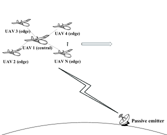
Figure 1: Multi-UAV passive localization system.

As illustrated in Fig.1, $N$ UAVs cooperate to compute a single RF emitter in the area of interest (AOI). Among $N$ UAVs, there is one central UAV, who works as a center of aggregating and processing information from other UAVs. The central UAV’s serial number is $1$ while the edge UAVs’ serial numbers are from $2$ to $N$. Flying along the prearranged trajectory, each UAV independently measures the RSS from the target. The position of passive emitter is denoted as $\mathbf{s}=(x,y,z)$. The $i$-th edge UAV measures $M_{i}$ times along its trajectory. The position of the $i$-th UAV at the $j$-th measurement is denoted as $\mathbf{u}_{i,j}=(x_{i,j},y_{i,j},z_{i,j})~{}1\leq i\leq N,1\leq j\leq M_{i}$. The time interval between any adjacent two sample point on the trajectory of UAV $i$ is $\Delta t_{j}$, $j=1,2,...,M_{i}-1$, and UAV $i$ flies at a velocity of $\mathbf{v}_{i,j}=[\mathbf{v}_{i,j,x},\mathbf{v}_{i,j,y},\mathbf{v}_{i,j,z}]$ at $\Delta t_{j}$. Then position of UAV $i$ at the $j$-th measurement can be represented by the position and velocity information of previous time as

$$\mathbf{u}_{i,j}=\mathbf{u}_{i,1}+\sum_{k=1}^{j-1}\Delta t_{k}\mathbf{v}_{i,k}$$ (1)

The distance from the $j$-th measurement time of UAV $i$ to the target can be expressed as

$$d_{i,j}=\sqrt{(x-x_{i,j})^{2}+(y-y_{i,j})^{2}+(z-z_{i,j})^{2}},$$

$$~{}~{}1\leq i\leq N~{}~{}1\leq j\leq M_{i}.$$ (2)

According to radio propagation path loss model (in decibels) [2], the received power of the $j$-th measurement time of UAV $i$ can be written as

$$P_{i,j}=f_{i,j}(\mathbf{s})+\eta_{i,j},~{}f_{i,j}(\mathbf{s})\triangleq P_{0}-10\gamma_{i}\lg(\frac{d_{i,j}}{d_{0}}).$$ (3a)

where $P_{0}$ denotes the power of source at reference distance $d_{0}$. $\gamma_{i}$ is the path loss exponent (PLE). The log-normal shadowing term $\eta_{i,j}$ is a Gaussian random variable with mean zero and variance $\sigma_{i,j}$.

Stacking all measurement values of UAV $i$ forms a $M_{i}$-dimensional column vector as follows

$$\mathbf{P}_{i}=\mathbf{f}_{i}(\mathbf{s})+\mathbf{\eta}_{i}.$$ (4)

which yields the probability density function (pdf)

$$Q_{i}(\mathbf{s})=\frac{1}{(2\pi)^{\frac{M_{i}}{2}}|\mathbf{N}_{i}|}\exp\{(\mathbf{r}_{i}-\mathbf{f}_{i}(\mathbf{s}))^{T}\mathbf{N}_{i}^{-1}(\mathbf{r}_{i}-\mathbf{f}_{i}(\mathbf{s}))\},$$

where $\mathbf{N}_{i}=\sigma_{i}\mathbf{I}_{M_{i}\times M_{i}}$ is the covariance matrix of $\mathbf{\eta}_{i}$.

Assuming measurement noises of different UAVs are dependent, the joint pdf of all UAVs is given by

$$Q(\mathbf{s})= \frac{1}{(2\pi)^{\frac{\sum_{i=1}^{N}M_{i}}{2}}\prod_{i=1}^{N}|\mathbf{N}_{i}|}$$

$$\exp\{\sum_{i=1}^{N}(\mathbf{r}_{i}-\mathbf{f}_{i}(\mathbf{s}))^{T}\mathbf{N}_{i}^{-1}(\mathbf{r}_{i}-\mathbf{f}_{i}(\mathbf{s}))\}.$$ (6)

The centralized maximum likelihood of $\mathbf{s}$ is in the form of

$$\max_{\mathbf{s}}~{}~{}Q(\mathbf{s})$$

$$\text{s. t.}~{}~{}~{}\mathbf{s}\in\mathrm{A}$$ (7)

where $\mathrm{A}$ represents the area of interest. However, this approach requires all edge UAVs to transmit measurement data to the central UAV. This will generate a heavy communication overhead.

III Proposed communication-efficiency distributed localization methods

To address the problem of heavy communication overhead from centralized approach, the design of high-communication-efficiency distributed methods is very important. In this section, two distributed communication-efficiency methods are proposed as follows: DMM and DEF. Finally, the communication overhead and computational complexity are analysed.

III-A Proposed DMM

In this subsection, we solve the RSS localization problem by MM algorithm in a distributed way. MM algorithm is a problem-driven algorithm that can take advantage of the problem structure. The key step to MM is constructing a surrogate function. By choosing surrogate function based on second order Taylor expansion, the MM can be implemented separably. In this way, the objective function at the $k$-th iteration in (II) can be upper bounded as

$$Q(\mathbf{s})\leq Q(\mathbf{s}^{k})+\mathbf{b}^{kT}(\mathbf{s}-\mathbf{s}^{k})+\frac{1}{2}(\mathbf{s}-\mathbf{s}^{k})^{T}\mathbf{M}(\mathbf{s}-\mathbf{s}^{k}),$$ (8)

where $\mathbf{s}^{k}$ is a constant and $\mathbf{b}^{k}=\nabla Q(\mathbf{s}^{k})$ stands for the corresponding gradient vector of objective $Q(\mathbf{s})$. Matrix $\mathbf{M}$ should satisfy the condition $\mathbf{M}\geq\nabla^{2}Q(\mathbf{s}),\forall\mathbf{s}\in\mathrm{A}$.

Clearly, for a sufficiently large value of $\mathbf{M}$ large enough, the condition is naturally satisfied. But the corresponding updating size at each iteration is small, casing a huge number of iterations. In order to find a proper $\mathbf{M}$, we make an approximation to (4) as follows

$$\tilde{d}_{i,j}\approx||\mathbf{u}_{i,j}-\mathbf{s}||_{2},$$ (9)

where $\tilde{d}_{i,j}=10^{\frac{P_{0}-P_{i,j}}{10\gamma_{i}}}d_{0}$. According to the least-squares (LS) criterion, the optimization problem in (II) is reformulated as

$$\mathop{\min}_{\mathbf{s}}Q(\mathbf{s})=\sum_{i=1}^{N}\sum_{j=1}^{M_{i}}(\tilde{d}_{i,j}-||\mathbf{u}_{i,j}-\mathbf{s}||_{2})^{2}.$$ (10)

After calculation, we have

$$\nabla^{2}Q(\mathbf{s})= 2\sum_{i=1}^{N}\sum_{j=1}^{M_{i}}(1-\frac{\tilde{d}_{i,j}}{||\mathbf{u}_{i,j}-\mathbf{s}||_{2}})\mathbf{I}$$ (11)

$$+\frac{\tilde{d}_{i,j}}{||\mathbf{u}_{i,j}-\mathbf{s}||_{2}^{3}}[(\mathbf{s}-\mathbf{u}_{i,j})(\mathbf{s}-\mathbf{u}_{i,j})^{T}],$$

and

$$\mathbf{b}_{i}^{k}=\sum_{j=1}^{M_{i}}2(||\mathbf{u}_{i,j}-\mathbf{s}^{k}||_{2}-\tilde{d}_{i,j})\frac{\mathbf{s}^{k}-\mathbf{u}_{i,j}}{||\mathbf{s}^{k}-\mathbf{u}_{i,j}||_{2}},$$ (12)

where $k$ represents the $k$-th iteration and $\mathbf{s}^{k}$ is the initial value corresponding the $k$-th iteration. Let us define matrix $\mathbf{M}$ as follows

$$\mathbf{M}=\lambda_{max}(\mathbf{\nabla^{2}Q(\mathbf{s})})\mathbf{I}=2K\mathbf{I},$$ (13)

where $K=\sum_{i=1}^{N}M_{i}$. It is noted that $\mathbf{M}$ is only related to the total measurement times.

Finally, we make a summary of the procedure of the DMM algorithm. This method is composed of local updating step and fusion step. In the $(k+1)$-th iteration, UAVs update locally based on $\mathbf{s}_{c}^{k}$ from the central UAV $1$ given by

$$\mathbf{s}_{i}^{k+1}=\mathbf{s}_{c}^{k}-\frac{N}{2K}\mathbf{b}_{i}^{k}.$$ (14)

Then, the central UAV $1$ collects all $\mathbf{s}_{i}^{k+1}$ from edge UAVs to generate the new value as follows

$$\mathbf{s}_{c}^{k+1}=\frac{1}{N}(\mathbf{s}_{1}^{k+1}+\sum_{i=2}^{N}\mathbf{s}_{i}^{k+1}),$$ (15)

which should be sent back to all UAVs. Repeating the above process until the terminal criterion is reached.

III-B Proposed DEF

To further reduce the communication overhead, we extend the distributed estimation scheme in [12] to our multi-UAV localization with a completely different weight coefficients. In our scheme, each edge UAV only needs to send local estimation and the weighting coefficient to the central UAV $1$. The central UAV fuses the local estimates to produce the final result. Here, the reliable grid search with length size $\Delta d$ is selected as the local solver.

In the local estimation stage, the estimation of the $i$-th UAV, denoted as $\hat{\mathbf{s}}_{i}$, is from its own measurements. The estimation is treated as an observation of the true position

$$\hat{\mathbf{s}}_{i}=\mathbf{s}+\mathbf{\xi}_{i},$$ (16)

where $\mathbf{\xi}_{i}$ is the estimate error with the covariance matrix denoted as $\mathbf{J}_{i}$, related to the specific local solver. Due to the use of unbiased grid search, we have $\mathbb{E}\{\mathbf{\xi}_{i}\}=\mathbf{0}$, $Cov(\mathbf{s},\mathbf{\xi}_{i})=\mathbf{0}$. Collecting all the distributed estimations yields a n-dimensional vector as follows

$$\hat{\mathbf{s}}=\mathbf{H}\mathbf{s}+\mathbf{\xi},~{}~{}\mathbf{H}\triangleq[\mathbf{I}_{3},\mathbf{I}_{3},\cdots,\mathbf{I}_{3}].$$ (17)

Under the assumption that all UAV’s estimation errors are independent with each other, the covariance matrix of $\mathbf{\xi}$ denoted as $\mathbf{J}$ is a diagonal matrix with the $i$-th diagonal element being $\mathbf{J_{i}}$. According to the best linear unbiased estimation (BLUE) principle, the most reliable fusion implemented in the central UAV $1$ is given by

$$\hat{\mathbf{s}}_{c} =(\mathbf{H}^{T}(\mathbf{J})^{-1}\mathbf{H})^{-1}\mathbf{H}^{T}(\mathbf{J})^{-1}\hat{\mathbf{s}}=\sum_{i=1}^{N}\underbrace{(\sum_{i=1}^{N}\mathbf{J}_{i}^{-1})^{-1}\mathbf{J}_{i}^{-1}}_{\mathbf{W}_{i}}\hat{\mathbf{s}}_{i}.$$

The final estimation $\hat{\mathbf{s}}_{c}$ is performed in the central UAV. However, it is hard to compute the weight coefficients directly while using complex algorithms in local estimation.A computable method is as follows

$$\mathbf{W}_{i} =(\sum_{i=1}^{N}\mathbf{J}_{i}^{-1})^{-1}\mathbf{J}_{i}^{-1}\approx(\sum_{i=1}^{N}\mathbf{C}_{i}^{-1})^{-1}\mathbf{C}_{i}^{-1}$$

$$=(\sum_{i=1}^{N}\mathbf{F}_{i})^{-1}\mathbf{F}_{i}\approx(\sum_{i=1}^{N}\mathbf{F}_{i}(\hat{\mathbf{s}}_{i}))^{-1}\mathbf{F}_{i}(\hat{\mathbf{s}}_{i}),$$ (19)

where $\mathbf{C}_{i}$ and $\mathbf{F}_{i}$ represents for the Cramer-Rao lower bound (CRLB) and the Fisher information matrix (FIM) of the $i$-th UAV’s estimation respectively. The last term is gotten by replacing the unattainable true position of target with the local estimation while calculating FIM. It is reasonable if the accuracies of local estimations are acceptable. The mean-square error of the final fusion in (III-B) is

$$MSE =\mathbb{E}\{||\hat{\mathbf{s}}_{c}-\hat{\mathbf{s}}||_{2}^{2}\}=\mathrm{Tr}(\sum_{i=1}^{N}\mathbf{W}_{i}^{T}\mathbf{J}_{i}\mathbf{W}_{i})$$

$$\geq\underbrace{((\sum_{i=1}^{N}\mathbf{C}_{i}^{-1})^{-1})}_{MSE^{F}_{\min}}=\mathrm{Tr}(\mathbf{F}^{-1}),$$ (20)

where the $\mathbf{F}$ represents the FIM of the centralized UAV,, fully utilizing all measurements from edge UAVs. The last term is from $\mathbf{F}\triangleq\sum_{i=1}^{N}\mathbf{F}_{i}$, as shown in (25).

Finally, we make a comparison between it and other distributed estimation methods. The minimum MSE of the estimator in [12] (called DEM) denoted as $MSE^{M}_{\min}$, is $(\sum_{i=1}^{N}(\mathrm{Tr}({\mathbf{C}_{i}))^{-1}})^{-1}$. Similarly, the minimum MSE of the average fusion (denoted as $MSE^{A}_{\min}$) is $\frac{1}{N}\mathrm{Tr}(\sum_{i=1}^{N}{\mathbf{C}_{i})}$. It is obvious that

$$MSE^{F}_{\min}\leq MSE^{M}_{\min}\leq\min\limits_{i}({MSE_{\min}(i)})\leq MSE_{\min}^{A}.$$ (21)

The third term represents that the best lower bound of estimations among edge UAVs before fusion. The second equality is achieved when $\mathbf{C}_{i}=\lambda\mathbf{I}$, where $\lambda$ is a constant. This condition is satisfied only when all edge UAVs are all in optimal geometry to target (deduced from [5]). Let us give an example: for a fixed target, the equiangular structure geometry is optimal using RSS measurements[5].

III-C Derivation of CRLB

In this section, we derive the CRLB of distributed multi-UAV trajectory localization. The FIM of the measurements from UAV $i$ and overall measurements are denoted as $\mathbf{F}_{i}$ and $\mathbf{F}$ respectively. The element in $a$-th row and $b$-th column of $\mathbf{F}_{i}$ is given by

$$\mathbf{e}_{i,ab}=-\mathbb{E}\{\frac{\partial^{2}\log{Q_{i}(\mathbf{s})}}{\partial\phi_{a}\partial\phi_{b}}\}=\sigma_{i}^{-1}\sum_{j=1}^{M_{i}}\frac{\partial P_{i,j}}{\partial\phi_{a}}\frac{\partial P_{i,j}}{\partial\phi_{b}},1\leq a,b\leq 3,$$ (22)

where

$$\frac{\partial P_{i,j}}{\partial\phi_{1}}=\frac{-10\gamma_{i}}{\ln(10)}\frac{x-(x_{1}+\sum_{k=1}^{j-1}\mathbf{v}_{i,k,x})}{d_{i,j}^{2}},$$ (23a)

$$\frac{\partial P_{i,j}}{\partial\phi_{2}}=\frac{-10\gamma_{i}}{\ln(10)}\frac{y-(y_{1}+\sum_{k=1}^{j-1}\mathbf{v}_{i,k,y})}{d_{i,j}^{2}},$$ (23b)

$$\frac{\partial P_{i,j}}{\partial\phi_{3}}=\frac{-10\gamma_{i}}{\ln(10)}\frac{z-(z_{1}+\sum_{k=1}^{j-1}\mathbf{v}_{i,k,z})}{d_{i,j}^{2}}.$$ (23c)

The element in the $a$-th row and the $b$-th column of $\mathbf{F}$ is given by

$$e_{ab}=-\mathbb{E}\{\frac{\partial^{2}\log{Q(\mathbf{s})}}{\partial\phi_{a}\partial\phi_{b}}\}=\sum_{i=1}^{N}\sigma_{i}^{-1}\sum_{j=1}^{M_{i}}\frac{\partial P_{i,j}}{\partial\phi_{a}}\frac{\partial P_{i,j}}{\partial\phi_{b}}=\sum_{i=1}^{N}e_{i,ab}.$$ (24)

The relationship between $\mathbf{F}$ and $\mathbf{F}_{i}$ is obtained as follows

$$\mathbf{F}=\sum_{i=1}^{N}\mathbf{F}_{i}.$$ (25)

Finally, the CRLB of distributed multi-UAV trajectory localization is expressed as

$$\mathbf{C}=\frac{\mathrm{Tr}(\mathbf{F})^{-1}}{\det{\mathbf{F}}}=\frac{\sum_{a,b=1,a\neq b}^{3}(e_{aa}e_{bb}-e_{ab}^{2})}{\tau},$$ (26)

where $\tau=e_{1,1}(e_{2,2}e_{3,3}-e_{2,3}^{2})-e_{1,2}(e_{1,2}e_{3,3}-e_{1,3}e_{2,3})+e_{1,3}(e_{1,2}e_{2,3}-e_{1,3}e_{2,2})$.

III-D Communication overhead and Computational Complexity Analysis

Now, let us make a complete analysis concerning communication overheads and computational complexities of the proposed two methods: DMM and DEF combing local search with distributed GN[9] and DEM[12] combing local search as performance benchmarks. Here, $\tau$ represents the dimension of the position vector, $p$ denotes the number of quantization bits of one element of position vector and $q$ denotes the number of bits of single weighting coefficient. $k_{1}$ denotes the total iteration number of DMM where $k_{2}$ denotes the required number of iterations of DGN to achieve convergence. The total number of required transmit bits, denoted as $\mathcal{B}$, are given by

$$\mathcal{B}_{DMM}=2(N-1)(\tau p)k_{1},$$ (27)

$$\mathcal{B}_{DGN}=(N-1)(2\tau p+\tau^{2}q)k_{2},$$ (28)

$$\mathcal{B}_{DEF}=(N-1)(\tau p+\tau^{2}q),$$ (29)

$$\mathcal{B}_{DEM}=(N-1)(\tau p+q).$$ (30)

The floating-point operations (FLOPs) of the above four methods are given by

$$\mathcal{C}_{D-MM}=\mathcal{O}(3\tau)\sum_{i=1}^{N}M_{i}k_{1},$$ (31)

$$\mathcal{C}_{D-GN}=\mathcal{O}(5\tau^{2}+5\tau)\sum_{i=1}^{N}M_{i}k_{2},$$ (32)

$$\mathcal{C}_{DEF}=\mathcal{O}(3\tau)\sum_{i=1}^{N}M_{i}(\frac{l}{\Delta d})^{\tau},$$ (33)

$$\mathcal{C}_{DEM}=\mathcal{O}(3\tau)\sum_{i=1}^{N}M_{i}(\frac{l}{\Delta d})^{\tau}.$$ (34)

IV Simulations and Discussions

In this section, we evaluate performance of the proposed distributed methods by simulations. The target is unknown in a $12\mathrm{km}\times 12\mathrm{km}$ AOI. System parameters are set as follows: $\gamma=3$, $\sigma^{2}=6\mathrm{dB}$, the number of samples per UAV is $8$. Each UAV flies over the AOI with flight altitude $h=60\mathrm{m}$.

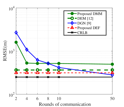
Figure 2: RMSE versus communication rounds between edge UAVs and the central UAV

Fig. 2 plots the curves of RMSE versus the rounds of communication between edge UAVs and the central UAV, namely iterations. From Fig. 2, it can be seen that the proposed distributed DMM and DEF converges rapidly, with lower rounds of communications, compared with DGN. The $\Delta d$ in DEF/DEM is $200\mathrm{m}$. Thus the proposed methods are of high communication-efficiency. Besides, the number of transmitted bits of DGN is almost $3$ times than that of proposed distributed DMM and DEF at each round. According to (31), (32), (33) and (34), the proposed DEF has a higher computational complexity, but it needs only one round of communication. In other words, it possesses the highest communication efficiency among four distributed methods. Although DEM also needs one round of communications. The DEM is worse than our proposed DEF in terms of RMSE performance.

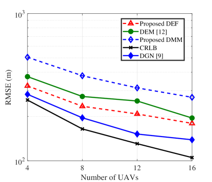
Figure 3: RMSE versus the number of UAVs

Fig. 3 demonstrates the curves of RMSE versus the number of edge UAVs. As the number of UAVs increases, the RMSE performances of all methods including DMM, DEF, DGN and DEM increases gradually. They have an increasing order on performance as follows: proposed DMM, DEM, proposed DEF, DGN. Thus, we can make a conclusion that the proposed DMM strikes a good balance among performance, computational complexity and communication efficiency.

V Conclusion

In our work, a RSS-based multi-UAV localization model utilizing trajectory has been established to find the position of passive source and the corresponding CRLB has been derived. To lower communication overhead, two high-communication-efficient distributed methods, DMM and DEF, have been proposed to exploit multiple UAVs and UAV trajectories. The simulation results have shown that the proposed DMM strikes a good balance among performance, computational complexity, and communication efficiency while the proposed DEF is one of the two highest communication-efficiency methods among distributed methods DEF, DMM, DEM, and DGN. Moreover, the proposed DEF performs better than DEM in terms of RMSE and has the same communication efficiency as the latter.

References

- [1] F. Gustafsson and F. Gunnarsson, “Mobile positioning using wireless networks: possibilities and fundamental limitations based on available wireless network measurements,” IEEE Signal Process. Mag., vol. 22, no. 4, pp. 41–53, 2005.
- [2] A. J. Weiss, “On the accuracy of a cellular location system based on RSS measurements,” IEEE Trans. Veh. Technol., vol. 52, no. 6, pp. 1508–1518, 2003.
- [3] F. Shu, S. Yang, Y. Qin, and J. Li, “Approximate analytic quadratic-optimization solution for TDOA-based passive multi-satellite localization with earth constraint,” IEEE Access., vol. 4, pp. 9283–9292, 2016.
- [4] D. Kim, K. Lee, M. Park, and J. Lim, “UAV-based localization scheme for battlefield environments,” in MILCOM 2013 - 2013 IEEE Military Communications Conference, 2013, pp. 562–567.
- [5] S. Xu, Y. Ou, and W. Zheng, “Optimal sensor-target geometries for 3-D static target localization using received-signal-strength measurements,” IEEE Signal Process. Lett., vol. 26, no. 7, pp. 966–970, 2019.
- [6] K. Dogancay, “UAV path planning for passive emitter localization,” IEEE Trans. Aerosp. Electron. Syst., vol. 48, no. 2, pp. 1150–1166, 2012.
- [7] Y. Li, F. Shu, B. Shi, X. Cheng, Y. Song, and J. Wang, “Enhanced RSS-based uav localization via trajectory and multi-base stations,” IEEE Commun Lett., pp. 1–1, 2021.
- [8] G. C. Calafiore, L. Carlone, and M. Wei, “A distributed technique for localization of agent formations from relative range measurements,” IEEE Trans. Syst., Man, Cybern. A, Syst.,Humans., vol. 42, no. 5, pp. 1065–1076, 2012.
- [9] T. Zhao and A. Nehorai, “Information-driven distributed maximum likelihood estimation based on gauss-newton method in wireless sensor networks,” IEEE Trans. Signal. Proces., vol. 55, no. 9, pp. 4669–4682, 2007.
- [10] G. Soatti, M. Nicoli, S. Savazzi, and U. Spagnolini, “Consensus-based algorithms for distributed network-state estimation and localization,” IEEE Trans. Signal Inf. Process. Netw., vol. 3, no. 2, pp. 430–444, 2017.
- [11] C. Y. Chong, “Hierarchical estimation,” in Proceedings of 2nd MIT/ONR Workshop on Distributed Information and Decision Systems Motivated by Naval Command Control and Communication (C3) Problems, 1979.
- [12] Y. Fu and Z. Tian, “Cramer-Rao bounds for hybrid TOA/DOA-based location estimation in sensor networks,” IEEE Signal Process. Lett., vol. 16, no. 8, pp. 655–658, 2009.
- [13] S. Wang, B. R. Jackson, S. Rajan, and F. Patenaude, “Received signal strength-based emitter geolocation using an iterative maximum likelihood approach,” in MILCOM 2013 - 2013 IEEE Military Communications Conference, 2013, pp. 68–72.
- [14] F. Shu, Y. Qin, T. Liu, L. Gui, Y. Zhang, J. Li, and Z. Han, “Low-complexity and high-resolution DOA estimation for hybrid analog and digital massive MIMO receive array,” IEEE Trans. Commun., vol. 66, no. 6, pp. 2487–2501, 2018.