Abstract

An important class of structural models studies the determinants of skill formation and the optimal timing of interventions. In this paper, I provide new identification results for these models and investigate the effects of seemingly innocuous scale and location restrictions on parameters of interest. To do so, I first characterize the identified set of all parameters without these additional restrictions and show that important policy-relevant parameters are point identified under weaker assumptions than commonly used in the literature. The implications of imposing standard scale and location restrictions depend on how the model is specified, but they generally impact the interpretation of parameters and can affect counterfactuals. Importantly, with the popular CES production function, commonly used scale restrictions are overidentifying and lead to biased estimators. Consequently, simply changing the units of measurements of observed variables might yield ineffective investment strategies and misleading policy recommendations. I show how existing estimators can easily be adapted to solve these issues. As a byproduct, this paper also presents a general and formal definition of when restrictions are truly normalizations.

1 Introduction

Structural models are key tools of economists to simulate changes in the economic environment and evaluate and design policies. An important class of such models deals with skill and human capital formation. Human capital formation is a main part of many structural models and is an important driver of economic growth and inequality [Murphy and TopelMurphy and Topel2016], which makes policies targeting skill formation particularly critical. This growing literature estimates production functions of various skills of children, studies how past skills, parental skills, and investments affect future skills, and links the skills to outcomes in adulthood. The results can, among others, be used to inform about determinants of skill formation, timing of investments in children, and optimal interventions for disadvantaged children. Following the seminal papers of CH:08 and CHS:10, a large literature has studied different specifications with data sets from several countries and has provided many important policy recommendations.

A major challenge in these models is that skills are not directly observable, do not have a natural scale, and can only be approximated through measurements, such as test scores. Identification in these models is often achieved in two steps, where the distribution of skills is identified from the measurements in the first step and the production function is identified in the second step (see for example CHS:10, AMNS:17, and AMN:19). To obtain point identification in the first step, researchers have to impose restrictions that fix the unknown scales and locations of the skills. While these restrictions are necessary to achieve point identification when studying the first step in isolation, it is not clear whether these restrictions are needed once all other restrictions of the model are combined.

In this paper, I present a new identification analysis for skill formation models and investigates the consequences of the seemingly innocuous normalizations. Instead of providing sufficient conditions for point identification using multi-step arguments, I start by pooling all parts of the model and characterize the identified set of all parameters without the scale and location restrictions. This characterization highlights which parameters are point or partially identified and how additional restrictions affect the identified set. In particular, I show that many key features are invariant to these restrictions, are point identified without them, and are identified under weaker assumptions than commonly used in the literature (e.g. they do not require age-invariant measures). These identification results hold for both parametric and nonparametric versions of the model.

The exact implications of imposing the additional scale and location restrictions on parameters and counterfactuals depends on how the model is specified and what the object of interest is. Specifically, a restriction could be a harmless normalization with one production function, but could impose strong assumptions with a different one. I therefore analyze two popular specifications, namely the trans-log production function (which includes Cobb-Douglas as a special case) and the CES production function. For the trans-log production function, it turns out that standard scale and location restrictions are necessary for point identification of the parameters and are not overidentifying, but still affect production function parameter estimates and certain counterfactuals. Since these restrictions are often arbitrary and depend on the units of measurement of the data, the estimates are hard to interpret, difficult to compare across different studies, and policy recommendations based on such counterfactuals can be misleading. For the CES case with different parametric assumptions, I show that commonly used scale restrictions are in fact overidentifying and imposing them severely impacts the estimated parameters of the model. Simply changing the units of measurements of one of the skill measures (for example from years to months) can then lead to different estimated dynamics in the model, it can change the estimated persistence of skills and the effects of parental investments on skill formation, and it can yield ineffective optimal investment strategies.

Next to providing new identification results, I also show how existing estimators can easily be adapted to solve these overidentification issues. While many parameters are still hard to interpret, the estimates can then be used to calculate point identified features and counterfactuals that are invariant to the scale and location restrictions and the units of measurement of the data. I illustrate the results using Monte Carlo simulations based on the setup and the estimator of AMN:19.

In this particular class of models, the scale and location restrictions are generally not innocuous normalizations. More generally, to the best of my knowledge, there does not exist a formal definition of when a restriction is truly a normalization, and I provide one in this paper. Clearly, any restriction on the parameters of the model affects some of the estimates and thus, a normalization has to be with respect to some function or feature of interest, such as a subvector or a counterfactual prediction. I therefore define a restriction as a normalization if imposing the restriction does not change the identified set of a function of interest. I illustrate this definition in a simple and commonly used example and use it as a basis for the analysis of skill formation models.

A broader takeaway from this paper is that researchers need to carefully check if imposed restrictions are in fact normalizations, which is especially important in structural models where identification proceeds in multiple steps and supposedly innocuous restrictions in one step might have unintended consequences in subsequent steps. Researchers should then focus on features of the model that are invariant to the restrictions. If estimates depend the these types of restrictions, as in skill formation models, resulting policy recommendations might be ineffective and results might not be comparable across different studies. In addition, the estimates might then not be suitable ingredients to calibrate larger models, as in Daruich:18, unless one can argue that all main conclusions are unaffected by the restrictions.

Literature: Following the influential work of CH:08 and CHS:10, a growing literature has emerged that studies the development of latent variables. For example, HP:11 study the determinants of children’s cognitive and non-cognitive skills using Indian data, FK:14 investigate how the time allocation affects cognitive and noncognitive development using Australian data, AMN:19 and AMNS:17 estimate the effects of health and cognition on human capital with data from India and Ethiopia and Peru, respectively, and ACDMR:19 study which early childhood intervention led to significant gains in cognitive and socio-emotional skills among disadvantaged children using Colombian data. The literature has provided many important insights regarding the nature of persistence, dynamic complementarities between the different components, and the optimal targeting of interventions. See also CH:07, CH:09, Cunha:11, HPS:13, AJ:16, HAP:17, and references therein.

In these papers, the measurement system for the latent variables is assumed to have a factor structure. Thus, to identify the joint distribution, certain restrictions on the measurement system are needed, which typically fix the scale and the location of the latent variables, either in the first period or by “anchoring” them to an adult outcome. In particular, CH:08 study a model where the production function is log-linear. Their identification arguments proceed in two steps. First, they identify the distribution of skills using the measurement system and an adult outcome anchor to obtain a well-defined scale and location. Using that distribution, they identify the production function in the second step. They also discuss which parameters depend on the anchor or its units of measurement. In this particular model, I illustrate that certain policy relevant parameters, such as optimal investment sequences, can depend on the specific scales and the specific units of the measurements of the observed variables. Additionally, I show that a set of key features that can be expressed in terms of quantiles of the skill distribution are identified under weaker restrictions on the measures and the production function and without anchoring the skills or fixing their scales. Importantly, I also provide formal identification results for other production technologies, such as the popular CES production function, where standard restrictions have much more severe consequences. In particular, certain scale restrictions are not needed for identification and imposing them through an initial period normalization or through anchoring leads to inconsistent estimators.

Common restrictions are to fix the scales and locations of each latent factor in each time period by setting parameters in the measurement system. If they are set to the same values in all time periods, Agostinelli and Wiswall (2016a, 2016b, 2022) refer to this restriction as an age-invariance assumption (see Assumption 3(a) for a formal definition or Definition 1 of Agostinelli and Wiswall (2022)). In an important contribution, Agostinelli and Wiswall (2016a, 2016b, 2022) show that imposing this age-invariance assumption can yield overidentifying restrictions and inconsistent estimators when the production function has a known scale and location. They then discuss relaxations of popular production functions when the measures are age-invariant. They also show that without age-invariant measures, production function restrictions can still yield point identification (see Corollary 1 below and the related discussion). In both cases, they still impose scale and location restrictions on the skill measures in the first period, and they argue that these restrictions are necessary for point identification. While this is true for the trans-log production function that they use in their empirical application, these scale restrictions are not required for the CES production function and imposing them yields inconsistent estimators. Moreover, I show that, in general, production function parameters and certain counterfactuals can depend on the specific scales and the specific units of the measurements of the data. With restrictions on the production function, I also show that changing the scales of the skills can yield misleading dynamics. Again, many key parameters are invariant to these restrictions, including age-invariance, and are in fact point identified without them.

In independent research, DKP:20 have recently shown that, with a trans-log production function, anchored treatment effects are invariant to scale and location normalizations and are identified without age-invariance. They also show in simulations that standard restrictions lead to biased estimated treatment effects with the CES production function. In the trans-log case, these results are similar to those in part 4 of Theorem 2 below. While their proof is specific to the trans-log production function with a log-linear measurement error system, my arguments can easily be extended to other cases. In addition, my proof highlights that only skill measures in the first period are needed to identify anchored treatment effects, which reduces the data requirements considerably and consequently weakens the assumptions. I also consider additional policy-relevant features. For the CES case, I show that standard restrictions are overidentifying, which explains why their estimated treatment effects are biased, and describe how existing estimators can be adapted to solve this issue.

Consequences resulting from normalizations have been discussed in various contexts. In factor models, it is well known that restrictions are needed for point identification (see e.g. AR:56, Madansky:64, JG:75, and CH:08, among many others). Williams:20 shows that these restrictions are not needed for identification of certain features, such as the variance decomposition. I combine a factor model with a production function, which can reduce the number of additional restrictions needed. Many papers have argued that important features should not depend on normalizations and have shown this in specific examples, such as Freyberger:18 and KSSS:18. Similar to this paper, but in a very different context, AS:14 show that restrictions that were thought of as a normalization can lead to biases. KSS:20 show that certain counterfactuals in dynamic discrete choice models are identified, even when the model is not nonparametrically identified. RWZ:10 define a normalization in vector autoreggressive models to pin down unidentified signs; see end of Section 2 for more details. Matzkin (1994, 2007) discusses several examples of normalizations that can be used to achieve point identification, some of which are motivated by economic theory, but she does not present a definition. Lewbel:19 provides an informal discussion of normalizations, which is conceptually very similar to the formal definition below.

When normalizing restrictions are needed to point identify the parameters, there are often different ways of imposing them when estimating the model. Clever choice can then yield particularly convenient restrictions on the parameter space (as in GL:19) or even faster rates of convergence (as in CKK:15). See also HWZ:07 for a discussion on estimation with normalizations. In skill formation models, different restrictions can also yield observationally equivalent models with identical counterfactual, but certain specification might be easier to estimate.

Structure: In Section 2, I provide a formal definition of a normalization and a very simple illustrative example. Section 3 contains the identification analysis of different skill formation models and the Monte Carlo simulations. Section 4 extends some of the parametric identification results to a more general nonparametric setting.

2 Normalizations

I begin by providing a formal definition of a normalization, which will serve as a basis for the analysis of skill formation models. Suppose we have a model where $\theta_{0}\in\Theta$ denotes the true values of the parameters and $\Theta$ is the parameter space. Here $\theta_{0}$ could denote the coefficients in a regression model or the parameters in a skill formation model. If the model is nonparametric or semiparametric, $\theta_{0}$ could also contain unknown functions. Let $Z$ contain all observed random variables, such as $Y$ and $X$, with distribution $P(Z)$. For any $\theta\in\Theta$, the model generates a joint distribution of the data $Z$, denoted by $P(Z,\theta)$. Since the model is assumed to be correctly specified, the true distribution of $Z$ is $P(Z,\theta_{0})$. The model typically contains certain assumptions, such as functional form or independence assumptions, but suppose that so far none of the normalizations are imposed. We then say that $\theta_{1},\theta_{2}\in\Theta$ are observationally equivalent if they generate the same distribution of the data: $P(Z,\theta_{1})=P(Z,\theta_{2})$. The identified set for $\theta_{0}$ is

$$\Theta_{0}=\{\theta\in\Theta:P(Z,\theta)=P(Z)\}.$$

We say that $\theta_{0}$ is point identified if $\Theta_{0}$ is a singleton. Let $g(\theta_{0})$ be a (potentially vector-valued) function of interest, such as a counterfactual. The identified set for $g(\theta_{0})$ is

$$\Theta_{g_{0}}=\{g(\theta):\theta\in\Theta_{0}\}.$$

We say that $g(\theta_{0})$ is point identified if $\Theta_{g_{0}}$ is a singleton. Notice that if $\theta_{0}$ is point identified, then $g(\theta_{0})$ is point identified as well, but $g(\theta_{0})$ could be point identified even if $\theta_{0}$ is not.

In models with normalizations, $\Theta_{0}$ is typically not a singleton. A normalization is a restriction of the form $\theta\in\Theta_{N}$, where $\Theta_{N}\subseteq\Theta$ is a known set that does not depend on the distribution of the data. Hence, the normalization restricts the feasible values of $\theta$, such as setting one element to $1$. I define a restriction to be normalization if it does not change the identified set for some function $g(\theta_{0})$.

Definition 1.

The restriction $\theta\in\Theta_{N}$ is a normalization with respect to $g(\theta_{0})$ if for all $\theta_{0}\in\Theta$

$$\{g(\theta):\theta\in\Theta_{0}\cap\Theta_{N}\}=\{g(\theta):\theta\in\Theta_{0}\}.$$

Typically, $\Theta_{0}\cap\Theta_{N}$ is a singleton. That is, we achieve point identification once the normalizations are imposed. Since $\theta_{0}\in\Theta_{0}$, the definition then requires that

$$\{g(\theta_{0})\}=\{g(\theta):\theta\in\Theta_{0}\cap\Theta_{N}\}=\{g(\theta):\theta\in\Theta_{0}\}$$

and thus that $g(\theta_{0})$ is point identified, even without a normalization. In addition, since normalizations are often arbitrary, $\theta_{0}$ is usually not in $\Theta_{0}\cap\Theta_{N}$. Thus, the restriction $\theta\in\Theta_{N}$ is not a normalization with respect to $\theta_{0}$, but it can be a normalization with respect to particular functions of interest. Moreover, the restriction can be a normalization for some function and not for others. Hence, researchers need to argue that normalizations hold with respect to all functions of interest, such as all counterfactuals in a structural model.

The definition also implies that a normalization cannot impose any additional overidentifying restrictions in the sense that $\Theta_{0}\cap\Theta_{N}\neq\emptyset$ if $\Theta_{0}\neq\emptyset$. That is, if there is a parameter that is consistent with the model and the distribution of the data without the normalizations, then there is also such a parameter with the normalizations.

As a very simple illustrative example, consider the probit model

$$Y=\mathbf{1}(\beta_{0,1}+\beta_{0,2}X\geq U),$$

where $var(X)>0$, $U\mid X\sim N(\mu_{0},\sigma_{0}^{2})$ and $\sigma_{0}^{2}>0$. The true parameter vector is $\theta_{0}=(\beta_{0,1},\beta_{0,2},\mu_{0},\sigma_{0})^{\prime}$ and $Z=(Y,X)$. Now notice that

$$P(Y=1\mid X=x)=\Phi\left(\frac{\beta_{0,1}-\mu_{0}}{\sigma_{0}}+\frac{\beta_{0,2}}{\sigma_{0}}x\right),$$

where $\Phi$ denotes the standard normal cdf. Since $var(X)>0$, $\frac{\beta_{0,1}-\mu_{0}}{\sigma_{0}}$ and $\frac{\beta_{0,2}}{\sigma_{0}}$ are point identified. It is also well known and easy to see that

$$\Theta_{0}=\left\{\theta\in\mathbb{R}^{4}:\frac{\beta_{1}-\mu}{\sigma}=\frac{\beta_{0,1}-\mu_{0}}{\sigma_{0}}\text{ and }\frac{\beta_{2}}{\sigma}=\frac{\beta_{0,2}}{\sigma_{0}}\right\}$$

because all values in $\Theta_{0}$ imply the same joint distribution of $(Y,X)$.

Since $\theta_{0}$ is not point identified, a common normalization in this setting is $\mu=0$ and $\sigma=1$. Using the previous notation, this means that $\Theta_{N}=\mathbb{R}^{2}\times 0\times 1$ and

$$\Theta_{0}\cap\Theta_{N}=\left(\frac{\beta_{0,1}-\mu_{0}}{\sigma_{0}},\frac{\beta_{0,2}}{\sigma_{0}},0,1\right).$$

Clearly, this restriction is not a normalization with respect to $\beta_{0,1}$ or $\beta_{0,2}$, which are typically not objects of interest. In fact, in general $\theta_{0}\notin\Theta_{0}\cap\Theta_{N}$ unless $\mu_{0}=0$ and $\sigma_{0}=1$. However, this restriction is a normalization with respect to (potentially counterfactual) probabilities

$$P(Y=1\mid X=x)=\Phi\left(\frac{\beta_{0,1}-\mu_{0}}{\sigma_{0}}+\frac{\beta_{0,2}}{\sigma_{0}}x\right)$$

or, when $X$ is continuous, marginal effects

$$\frac{\partial}{\partial x}P(Y=1\mid X=x)=\frac{\partial}{\partial x}\Phi\left(\frac{\beta_{0,1}-\mu_{0}}{\sigma_{0}}+\frac{\beta_{0,2}}{\sigma_{0}}x\right).$$

Clearly, these features are point identified even though $\theta_{0}$ is not. While this is a very simple example, it highlights that normalizations affect parameters and, to get interpretable results, one needs to focus on features that are invariant to the restrictions. See also Lewbel:19 for additional discussion on normalizations and some other examples.

In the context of vector autoregressive models, RWZ:10 define a normalization as a restriction on the parameter space that pins down unidentified signs of coefficients. These restrictions are imposed in addition to other assumptions, such as long run restrictions. Just like above, their normalizations do not impose additional overidentifying restrictions. Unlike my definition, it is not clear whether these restrictions are without loss of generality in the sense that they do not affect functions of interest. If they do, they play the same role as the other assumptions and one would have to argue why they reasonable, in contrast to normalizations as defined in Definition 1.

3 Skill formation models

I now illustrate the subtle issues that can arise from normalizations in a model of skill formation. I start by introducing the general model and then discuss the results for the trans-log and the CES production functions.

3.1 Model

Let $\theta_{t}$ denote skills at time $t$ and let $I_{t}$ be investment at time $t$. We are interested in the roles of investment and past skills in the development of future skills. A complication in this setting is that skills and investment are not directly observed and we instead observe measurements of them, denoted by $Z_{\theta,t,m}$ and $Z_{I,t,m}$.

Specifically, I consider the model:

(1) $$\theta_{t+1} = f(\theta_{t},I_{t},\delta_{t},\eta_{\theta,t})\hskip 130.88268ptt=0,\ldots,T-1$$

(2) $$Z_{\theta,t,m} = \mu_{\theta,t,m}+\lambda_{\theta,t,m}\ln\theta_{t}+\varepsilon_{\theta,t,m}\hskip 73.97716ptt=0,\ldots,T,m=1,2$$

(3) $$Z_{I,t,m} = \mu_{I,t,m}+\lambda_{I,t,m}\ln I_{t}+\varepsilon_{I,t,m}\hskip 73.97716ptt=0,\ldots,T-1,m=1,2$$

The first equation describes the production technology with a production function $f$ that depends on skills and investment at time $t$, a parameter vector $\delta_{t}$, and an unobserved shock $\eta_{\theta,t}$. The second and the third equations describe the measurement system for unobserved (latent) skills $\theta_{t}$ and unobserved investment $I_{t}$, respectively. Observed investment is a special case with $\mu_{I,t,m}=0$, $\lambda_{I,t,m}=1$, and $\varepsilon_{I,t,m}=0$ for all $m$ and $t$ in which case $Z_{I,t,m}=\ln I_{t}$.

Next, I introduce two additional equations to allow for endogenous investment and to anchor the measures at an adult outcome. If investment is exogenous, in the sense that $\eta_{\theta,t}$ is independent of $I_{t}$, then these additional equations are not needed for the main identification results. That is, let

(4) $$\ln I_{t} = \beta_{0t}+\beta_{1t}\ln\theta_{t}+\beta_{2t}\ln Y_{t}+\eta_{I,t}\hskip 73.97716ptt=0,\ldots,T-1$$

(5) $$Q = \rho_{0}+\rho_{1}\ln\theta_{T}+\eta_{Q}$$

Here $Y_{t}$ is parental income (or another exogenous variable that affects investment) and $Q$ is an adult outcome, such as earnings or education. An adult outcome does not necessarily have to be available and we can simply use a skill measure in period $T$ in its place.

To summarize, the observed variables are the measures $\{Z_{\theta,t,m},Z_{I,t,m}\}_{t=0,\ldots,T,m=1,2}$, income $\{Y_{t}\}_{t=0}^{T-1}$ and the adult outcome $Q$, but we neither observe skills $\{\theta_{t}\}^{T}_{t=0}$ nor investment $\{I_{t}\}_{t=0}^{T-1}$. We also do not observe the measurement errors $\{\varepsilon_{\theta,t,m},\varepsilon_{I,t,m}\}_{t=0,\ldots,T,m=1,2}$ or $\eta_{\theta,t}$, $\{\eta_{I,t}\}_{t=0}^{T-1}$, and $\eta_{Q}$. The parameters of the model are $\{\mu_{\theta,t,m},\lambda_{\theta,t,m}\}_{t=0,\ldots,T,m=1,2}$, $\{\mu_{I,t,m},\lambda_{I,t,m}\}_{t=0,\ldots,T-1,m=1,2}$, $\{\delta_{t}\}^{T-1}_{t=0}$, $\{\beta_{0t},\beta_{1t},\beta_{2t}\}^{T-1}_{t=0}$, and $(\rho_{0},\rho_{1})$.

In the following analysis, I consider two forms for the production technology (1). These two forms have been the most extensively used and estimated in the empirical literature:

• Trans-log:

  $$\ln\theta_{t+1}=a_{t}+\gamma_{1t}\ln\theta_{t}+\gamma_{2t}\ln I_{t}+\gamma_{3t}\ln\theta_{t}\ln I_{t}+\eta_{\theta,t}$$

  with $\delta_{t}=(a_{t},\gamma_{1t},\gamma_{2t},\gamma_{3t})$.

• Constant Elasticity of Substitution (CES):

  $$\theta_{t+1}=(\gamma_{1t}\theta_{t}^{\sigma_{t}}+\gamma_{2t}I_{t}^{\sigma_{t}})^{\psi_{t}/\sigma_{t}}\exp(\eta_{\theta,t})$$

  with $\delta_{t}=(\gamma_{1t},\gamma_{2t},\sigma_{t},\psi_{t})$.

When $\gamma_{3t}=0$, the trans-log reduces to the Cobb-Douglas production function. I now state several additional assumptions that are common in the literature.

Assumption 1.

1. $\{\{\varepsilon_{\theta,t,m}\}_{t=0,\ldots,T,m=1,2},\{\varepsilon_{I,t,m}\}_{t=0,\ldots,T-1,m=1,2},\eta_{Q}\}$ are jointly independent and independent of $\{\{\theta_{t}\}^{T}_{t=0},\{I_{t}\}_{t=0}^{T-1}\}$ conditional on $\{Y_{t}\}_{t=0}^{T-1}$.

2. All random variables have bounded first and second moments.

3. $E[\varepsilon_{\theta,t,m}]=E[\varepsilon_{I,t,m}]=E[\varepsilon_{Q}]=0$ for all $t$ and $m$.

4. $\lambda_{\theta,t,m},\lambda_{I,t,m}\neq 0$ for all $t$ and $m$.

5. For all $t\in\{0,\ldots,T\}$, $cov(\ln\theta_{t},\ln I_{s})\neq 0$ for some $s\in\{0,\ldots,T-1\}$ or $cov(\ln\theta_{t},\ln\theta_{s})\neq 0$ for some $s\in\{0,\ldots,T\}\backslash t$ . For all $t\in\{0,1,\ldots,T-1\}$, $cov(\ln I_{t},\ln\theta_{s})\neq 0$ for some $s\in\{0,\ldots,T\}$ or $cov(\ln I_{t},\ln I_{s})\neq 0$ for some $s\in\{0,\ldots,T-1\}\backslash t$.

6. For all $t$ and $m$ the real zeros of the characteristic functions of $\varepsilon_{\theta,t,m}$ are isolated and are distinct from those of its derivatives. Identical conditions hold for the characteristic functions of $\varepsilon_{I,t,m}$ and $\eta_{Q}$.

7. The support of $(\theta_{t},I_{t},Y_{t})$ includes an open ball in $\mathbb{R}^{3}$ for all $t$.

8. $E[\eta_{\theta,t}\mid\theta_{t},Y_{t}]=0$ and $E[\eta_{\theta,t}\mid\theta_{t},\eta_{I,t},Y_{t}]=\kappa_{t}\eta_{I,t}$ for all $t$.

Part (a) imposes common independence assumptions on the measurement errors. Importantly, $I_{t}$ and $\theta_{t}$ are not independent and $I_{t}$ may be endogenous and contemporaneously correlated with $\eta_{\theta,t}$. Part (b) is a standard restriction, part (c) is needed because all measurement equations contain an intercept, and part (d) ensures that the skills actually affect the measures. Part (e) requires that skills and investment are correlated in some time periods. Sufficient conditions are that $cov(\ln\theta_{t+1},\ln\theta_{t})\neq 0$ and $cov(\ln I_{t+1},\ln I_{t})\neq 0$ for all $t$. Notice that under parts (a) and (d) zero covariances of the latent variables are identified because, for example, $cov(\ln\theta_{t},\ln\theta_{s})=0$ if and only if $cov(Z_{\theta,t,1},Z_{\theta,s,1})=0$. Notice that I only require two measures in each period. One can drop this assumption by assuming that three measures are available. Part (f) contains weak regularity conditions needed for nonparametric identification of the distributions of skills and investment and that hold for most common distributions. Part (g) is a mild support condition that ensures sufficient variation of $(\theta_{t},I_{t},Y_{t})$ and rules out colinarity. Part (h) implies that $Y_{t}$ can serve as an instrument and identification can be achieved using a control function argument as in AMN:19. Linearity of the conditional mean function can be relaxed and one could allow for more flexible functional forms. Exogenous investment is a special case with $\kappa_{t}=0$.

Under parts (a)–(e) of Assumption 1 we get the following result.

Lemma 1.

Suppose that parts (a)–(e) of Assumption 1 hold. Then the joint distribution of

$$\left(\{\mu_{\theta,t,m}+\lambda_{\theta,t,m}\ln\theta_{t}\}_{t=0,\dots,T,m=1,2},\{\mu_{I,t,m}+\lambda_{I,t,m}\ln I_{t}\}_{t=0,\dots,T-1,m=1,2},\rho_{0}+\rho_{1}\ln\theta_{T}\right)$$

is point identified conditional on $\{Y_{t}\}_{t=0}^{T-1}$.

The proof follows from an extension of Kotlarski’s Lemma due to EW:12. Lemma 1 shows that under Assumption 1, we can identify the distribution of a linear combination of the log skills and investments, but not the parameters in equations (1)–(3), and therefore also not $\delta_{t}$. Below I discuss additional assumptions, which have been used in the literature, to achieve point identification of two sets of parameters: (i) the primitive parameters of the model (1)–(5): $\{\mu_{\theta,t,m},\lambda_{\theta,t,m}\}_{t=0,\ldots,T,m=1,2}$, $\{\mu_{I,t,m},\lambda_{I,t,m}\}_{t=0,\ldots,T-1,m=1,2}$, $\{\delta_{t}\}^{T-1}_{t=0}$, $\{\beta_{0t},\beta_{1t},\beta_{2t}\}^{T-1}_{t=0}$, and $(\rho_{0},\rho_{1})$ and (ii) “policy relevant” parameters, such as how changes in investment or income affect the adult outcome $Q$. I consider various combinations of assumptions and I discuss whether certain restrictions are normalizations.

There are two separate issues concerning identification and normalizations in this model. First, the previous literature has focused on sufficient conditions for point identification, which includes scale and location restrictions. However, it is unclear whether these restrictions are necessary or potentially overidentifying. If so, estimators are generally inconsistent. Second, once we have a set of restrictions that is non-overidentifying, it is important to understand which parameters and features are invariant to arbitrary scale and location restrictions. Although the implications in the CES case are more interesting, I start with the more transparent trans-log case in which only the second issue arises. As pointed out before, whether or not a restriction is a normalization depends on the specifics of the model, and we will see that certain parameters are invariant in some settings, but not in others.

3.2 Trans-log production function

In this section I consider the production function

$$\ln\theta_{t+1}=a_{t}+\gamma_{1t}\ln\theta_{t}+\gamma_{2t}\ln I_{t}+\gamma_{3t}\ln\theta_{t}\ln I_{t}+\eta_{\theta,t}.$$

I now introduce additional assumptions that are commonly used in the literature.

Assumption 2.

$\lambda_{\theta,0,1}=1$ and $\mu_{\theta,0,1}=0$.

Assumption 3.

1. $\lambda_{\theta,t,1}=\lambda_{\theta,t+1,1}$ and $\mu_{\theta,t,1}=\mu_{\theta,t+1,1}$ for all $t=0,\ldots,T-1$

2. $a_{t}=0$ and $\gamma_{1t}+\gamma_{2t}+\gamma_{3t}=1$ for all $t=0,\ldots,T-1$.

Assumption 4.

1. $\lambda_{I,t,1}=\lambda_{I,t+1,1}=1$ and $\mu_{I,t,1}=\mu_{I,t+1,1}=0$ for all $t=0,\ldots,T-2$.

2. $\beta_{0t}=0$ and $\beta_{1t}+\beta_{2t}=1$ for all $t=0,\ldots,T-1$.

Assumption 2 is usually thought of as a normalization, which is commonly imposed since log skills are only identified up to scale and location. Here, I impose the restrictions on the first measure, which is without loss of generality. Instead of fixing the intercept and the slope coefficient in equation (2) for $t=0$, one could set $\rho_{0}=0$ and $\rho_{1}=1$ and thus “anchor” the skills at $Q$. Assumption 2 anchors the skills at $Z_{\theta,0,1}$, but analogous issues discussed here also arise with anchoring at $Q$ (see Section 3.2.4 for details). Without such an assumption, the parameters are not point identified. Assumptions 3(a) states that the skill measures are age-invariant (using the terminology of AW:22 – see their Definition 1 and footnote 10). Assumption 3 imposes restrictions on the technology, which AW:22 refer to as a known scale and location assumption in a more general context. Assumption 4(a) states that an investment measure is age-invariant. Assumption 4(b) imposes constant return to scale of investment, which is a strong assumption needed for point identification of all parameters without age-invariant investment measures. If investment was observed (i.e. $Z_{I,t,m}=\ln I_{t}$), Assumption 4(a) is automatically satisfied.

I now characterize the identified set of the primitive parameters of the model under Assumption 1 only. I then discuss point identification under different combinations of Assumptions 1 – 4 and show that several policy relevant parameters are invariant to the restrictions in Assumption 2 and are in fact point identified under Assumption 1 only. Finally, I illustrate why Assumption 2 is in general not a normalization for the primitive parameters of the model as well as some policy relevant parameters.

3.2.1 Identification

Define

$$\tilde{\theta}_{t}=\exp(\mu_{\theta,t,1})\theta_{t}^{\lambda_{\theta,t,1}}$$

so that

$$\ln\tilde{\theta}_{t}=\mu_{\theta,t,1}+\lambda_{\theta,t,1}\ln\theta_{t}\qquad\text{ and }\qquad\ln\theta_{t}=\frac{\ln\tilde{\theta}_{t}-\mu_{\theta,t,1}}{\lambda_{\theta,t,1}}.$$

Similarly, define

$$\tilde{I}_{t}=\exp(\mu_{I,t,1})I_{t}^{\lambda_{I,t,1}}$$

We can then rewrite the trans-log production technology in terms of $\tilde{\theta}_{t}$ and $\tilde{I}_{t}$ because

$$\frac{\ln\tilde{\theta}_{t+1}-\mu_{\theta,t+1,1}}{\lambda_{\theta,t+1,1}}=a_{t}+\gamma_{1t}\frac{\ln\tilde{\theta}_{t}-\mu_{\theta,t,1}}{\lambda_{\theta,t,1}}+\gamma_{2t}\frac{\ln\tilde{I}_{t}-\mu_{I,t,1}}{\lambda_{I,t,1}}+\gamma_{3t}\frac{\ln\tilde{\theta}_{t}-\mu_{\theta,t,1}}{\lambda_{\theta,t,1}}\frac{\ln\tilde{I}_{t}-\mu_{I,t,1}}{\lambda_{I,t,1}}+\eta_{\theta,t}.$$

After rearranging, we can then rewrite equations (1)–(5) as

(6) $$\hskip 22.76219pt\ln\tilde{\theta}_{t+1} = \tilde{a}_{t}+\tilde{\gamma}_{1t}\ln\tilde{\theta}_{t}+\tilde{\gamma}_{2t}\ln I_{t}+\tilde{\gamma}_{3t}\ln\tilde{\theta}_{t}\ln I_{t}+\tilde{\eta}_{\theta,t}\hskip 22.76219ptt=0,\ldots,T-1$$

(7) $$Z_{\theta,t,m} = \tilde{\mu}_{\theta,t,m}+\tilde{\lambda}_{\theta,t,m}\ln\tilde{\theta}_{t}+\varepsilon_{\theta,t,m}\hskip 108.12047ptt=0,\ldots,T,m=1,2$$

(8) $$Z_{I,t,m} = \tilde{\mu}_{I,t,m}+\tilde{\lambda}_{I,t,m}\ln\tilde{I}_{t}+{\varepsilon}_{I,t,m}\hskip 108.12047ptt=0,\ldots,T-1,m=1,2$$

(9) $$\ln\tilde{I}_{t} = \tilde{\beta}_{0t}+\tilde{\beta}_{1t}\ln\tilde{\theta}_{t}+\tilde{\beta}_{2t}\ln Y_{t}+\tilde{\eta}_{I,t}\hskip 91.04881ptt=0,\ldots,T-1$$

(10) $$Q = \tilde{\rho}_{0}+\tilde{\rho}_{1}\ln\tilde{\theta}_{T}+\eta_{Q}$$

where the parameters in equation (6) are

$$\tilde{a}_{t}=\lambda_{\theta,t+1,1}a_{t}+\mu_{\theta,t+1,1}-\frac{\lambda_{\theta,t+1,1}}{\lambda_{\theta,t,1}}\mu_{\theta,t,1}\gamma_{1t}-\frac{\lambda_{\theta,t+1,1}}{\lambda_{I,t,1}}\mu_{I,t,1}\gamma_{2t}+\frac{\lambda_{\theta,t+1,1}}{\lambda_{\theta,t,1}\lambda_{I,t,1}}\mu_{I,t,1}\mu_{\theta,t,1}\gamma_{3t}$$

$$\tilde{\gamma}_{1t}=\frac{\lambda_{\theta,t+1,1}}{\lambda_{\theta,t,1}}\left(\gamma_{1t}-\frac{\mu_{I,t,1}}{\lambda_{I,t,1}}\gamma_{3t}\right),\;\;\tilde{\gamma}_{2t}=\frac{\lambda_{\theta,t+1,1}}{\lambda_{I,t,1}}\left(\gamma_{2t}-\frac{\mu_{\theta,t,1}}{\lambda_{\theta,t,1}}\gamma_{3t}\right),\;\;\tilde{\gamma}_{3t}=\frac{\lambda_{\theta,t+1,1}}{\lambda_{\theta,t,1}\lambda_{I,t,1}}\gamma_{3t}$$

with unobservable $\tilde{\eta}_{\theta,t}=\lambda_{\theta,t+1,1}{\eta}_{\theta,t}$, the parameters in the measurement equations (7) and (8) are $\tilde{\mu}_{\theta,t,1}=0$, $\tilde{\lambda}_{\theta,t,1}=1$, $\tilde{\mu}_{I,t,1}=0$, $\tilde{\lambda}_{I,t,1}=1$,

$$\tilde{\lambda}_{\theta,t,m}=\lambda_{\theta,t,m}/\lambda_{\theta,t,1},\quad\tilde{\mu}_{\theta,t,1}=\mu_{\theta,t,m}-\left(\lambda_{\theta,t,m}/\lambda_{\theta,t,1}\right)\mu_{\theta,t,1}$$

$$\tilde{\lambda}_{I,t,m}=\lambda_{I,t,m}/\lambda_{I,t,1},\quad\tilde{\mu}_{I,t,1}=\mu_{I,t,m}-\left(\lambda_{I,t,m}/\lambda_{I,t,1}\right)\mu_{I,t,1},$$

the parameters in equation (9) are

$$\tilde{\beta}_{0t}=\lambda_{I,t,1}{\beta}_{0t}+\mu_{I,t,1}-(\lambda_{I,t,1}/\lambda_{\theta,t,1})\mu_{\theta,t,1}{\beta}_{1t},\quad\tilde{\beta}_{1t}=(\lambda_{I,t,1}/\lambda_{\theta,t,1}){\beta}_{1t},\quad\tilde{\beta}_{2t}=\lambda_{I,t,1}{\beta}_{2t}$$

with unobservable $\tilde{\eta}_{I,t}=\lambda_{I,t,1}{\eta}_{I,t}$, and the parameters in equation (10) are

$$\tilde{\rho}_{0}=\rho_{0}-\frac{\rho_{1}\mu_{\theta,t,1}}{\lambda_{\theta,t,1}},\quad\tilde{\rho}_{1}=\frac{\rho_{1}}{\lambda_{\theta,t,1}}.$$

The following theorem characterizes the identified set of the finite dimensional parameters of the model.

Theorem 1.

Suppose Assumption 1 holds.

1. The identified set of $\{\mu_{\theta,t,m},\lambda_{\theta,t,m}\}_{t=0,\ldots,T,m=1,2}$, $\{\mu_{I,t,m},\lambda_{I,t,m}\}_{t=0,\ldots,T-1,m=1,2}$, $(\rho_{0},\rho_{1})$, $\{\beta_{0t},\beta_{1t},\beta_{2t}\}^{T-1}_{t=0}$, $\{a_{t},\gamma_{1t},\gamma_{2t},\gamma_{3t}\}^{T-1}_{t=0}$ consists of all vectors that yield the same values of $\{\tilde{\mu}_{\theta,t,m},\tilde{\lambda}_{\theta,t,m}\}_{t=0,\ldots,T,m=1,2}$, $\{\tilde{\mu}_{I,t,m},\tilde{\lambda}_{I,t,m}\}_{t=0,\ldots,T-1,m=1,2}$, $(\tilde{\rho}_{0},\tilde{\rho}_{1})$, $\{\tilde{\beta}_{0t},\tilde{\beta}_{1t},\tilde{\beta}_{2t}\}^{T-1}_{t=0}$, and $\{\tilde{a}_{t},\tilde{\gamma}_{1t},\tilde{\gamma}_{2t},\tilde{\gamma}_{3t}\}^{T-1}_{t=0}$ as the true parameter vectors.

2. Let $\{\bar{\mu}_{\theta,t,1},\bar{\lambda}_{\theta,t,1}\}_{t=0}^{T}$, $\{\bar{\mu}_{I,t,1},\bar{\lambda}_{I,t,1}\}_{t=0}^{T-1}$, be fixed constants with $\bar{\lambda}_{\theta,t,1},\bar{\lambda}_{I,t,1}\neq 0$ for all $t$. If in addition $\{{\mu}_{\theta,t,1},{\lambda}_{\theta,t,1}\}_{t=0}^{T}=\{\bar{\mu}_{\theta,t,1},\bar{\lambda}_{\theta,t,1}\}_{t=0}^{T}$ and $\{{\mu}_{I,t,1},{\lambda}_{I,t,1}\}_{t=0}^{T-1}=\{\bar{\mu}_{I,t,1},\bar{\lambda}_{I,t,1}\}_{t=0}^{T-1}$, then the identified set is a singleton.

The identified set of the primitive parameters consists of all parameters that satisfy certain restrictions, analogous to the probit model. The second part of the theorem shows that the parameters are indeed not point identified and that the sources of underidentification are the ambiguous scales and locations of skills and investments. For example, without additional assumptions, equations (1)–(5) and (6)–(10) are observationally equivalent. That is, we cannot distinguish between the skills $\theta_{t}$ and $\tilde{\theta}_{t}$ and the corresponding production function parameters. Even if investment was observed (and $\mu_{I,t,1}=0$ for all $t$), we can then only identify $(\lambda_{\theta,t+1,m}/\lambda_{\theta,t,m})\gamma_{1t}$, but not $\lambda_{\theta,t,m}$ and $\gamma_{1t}$ separately. Hence, we cannot distinguish between changes in the quality of the measurements ($\lambda_{\theta,t+1,m}/\lambda_{\theta,t,m}$) and changes in the technology (${\gamma}_{1t}$). For example, suppose $Z_{\theta,t,m}$ are test scores. We then cannot distinguish between all kids getting smarter or tests becoming easier. Similarly, we can at best identify $\gamma_{2t}$ up to scale, even with observed investment.

The theorem implies that all parameters are point identified under additional assumptions. These results are an extension of those in AW:22, who assume that investment is exogenous (in the sense that it is uncorrelated with $\eta_{\theta,t}$).

Corollary 1.

Suppose Assumptions 1 and 2 hold. Suppose either Assumption 3(a) or Assumption 3(b) holds. Suppose either Assumption 4(a) or Assumption 4(b) holds. Then all parameters are point identified.

The corollary also immediately implies that Assumptions 3(a) and 3(b) together impose overidentifying restrictions, which is one of the main contributions of Agostinelli and Wiswall (2016a, 2016b, 2022). As shown in Theorem 6 in the appendix and illustrated in examples below, if the model is correctly specified and Assumption 1 holds, then there always exist sets of parameters which are consistent with the data and satisfy Assumptions 1, 2, either 3(a) or 3(b), and either 4(a) or 4(b). These different sets of assumptions therefore impose no additional restrictions on the distribution of observables. While different sets of assumptions yield point identification and are observationally equivalent, the estimated primitive parameters are usually quite different, as illustrated in Section 3.2.3. Moreover, these results show that the primitive parameters are not point identified without Assumption 2. However, setting the initial scales and locations to other values changes the identified values.

3.2.2 Invariant parameters

I now show that while the primitive parameters are generally very sensitive to the scale and location restrictions, many objects of interest are in fact point identified under Assumption 1 only. To state the formal results below, let $Q_{\alpha}(\theta_{t})$ be the $\alpha$ quantile of the skill distribution at time $t$ and let $F_{\ln(\theta_{t+1})}(\cdot)$ be the distribution function of log-skills at time $t+1$.

Theorem 2.

Suppose Assumption 1 holds.

1. $F_{\ln\theta_{t+1}}(a_{t}+\gamma_{1t}\ln Q_{\alpha_{1}}(\theta_{t})+\gamma_{2t}\ln Q_{\alpha_{2}}(I_{t})+\gamma_{3t}\ln Q_{\alpha_{1}}(\theta_{t})\ln Q_{\alpha_{2}}(I_{t})+Q_{\alpha_{3}}(\eta_{\theta,t}))$ is point identified for all $\alpha_{1},\alpha_{2},\alpha_{3}\in(0,1)$.

2. Let

   $$\ln I_{t}(Y)=\beta_{0t}+\beta_{1t}\ln Q_{\alpha_{1}}(\theta_{t})+\beta_{2t}\ln Y+Q_{\alpha_{4}}(\eta_{I,t})$$

   Then $F_{\ln\theta_{t+1}}(a_{t}+\gamma_{1t}\ln Q_{\alpha_{1}}(\theta_{t})+\gamma_{2t}\ln I_{t}(Y)+\gamma_{3t}\ln Q_{\alpha_{1}}(\theta_{t})\ln I_{t}(Y)+Q_{\alpha_{3}}(\eta_{\theta,t}))$ is point identified for all $\alpha_{1},\alpha_{3},\alpha_{4}\in(0,1)$.

3. $P\left(Q\leq q\mid\theta_{s}=Q_{\alpha_{1}}(\theta_{s}),\{I_{t}=Q_{\alpha_{2t}}(I_{t})\}^{T-1}_{t=0},\{\eta_{\theta,t}=Q_{\alpha_{3t}}(\eta_{\theta,t})\}^{T-1}_{t=s}\right)$ is point identified for all $\alpha_{1},\{\alpha_{2t},\alpha_{3t}\}^{T-1}_{t=s}\in(0,1)$.

4. $P\left(Q\leq q\mid\theta_{s}=Q_{\alpha}(\theta_{s}),\{Y_{t}=y_{t}\}^{T-1}_{t=s}\right)$ is point identified for all $\alpha\in(0,1)$.

5. Suppose Assumption 3(a) also holds. Then $\gamma_{1t}+\gamma_{3t}\ln Q_{\alpha}(I_{t})$ is point identified for all $\alpha$ and $P(\gamma_{1t}+\gamma_{3t}\ln I_{t}\leq q)$ is point identified for all $q\in\mathbb{R}$.

The function $F_{\ln\theta_{t+1}}(a_{t}+\gamma_{1t}\ln Q_{\alpha_{1}}(\theta_{t})+\gamma_{2t}\ln Q_{\alpha_{2}}(I_{t})+\gamma_{3t}\ln Q_{\alpha_{1}}(\theta_{t})\ln Q_{\alpha_{2}}(I_{t})+Q_{\alpha_{3}}(\eta_{\theta,t}))$ measures how changes in investment changes the relative standing in the skill distribution. For example, consider an individual with $\theta_{t}=Q_{0.1}(\theta_{t})$, which means that the person is in the lowest $10\%$ of the skill distribution at time $t$. Then, given investment $I_{t}=Q_{0.25}(I_{t})$ and a median production function shock, $\eta_{\theta,t}=Q_{0.5}(\eta_{\theta,t})$,

$$F_{\ln\theta_{t+1}}(a_{t}+\gamma_{1t}\ln Q_{0.1}(\theta_{t})+\gamma_{2t}\ln Q_{0.25}(I_{t})+\gamma_{3t}\ln Q_{0.1}(\theta_{t})\ln Q_{0.25}(I_{t})+Q_{0.5}(\eta_{\theta,t}))$$

tells us the relative rank (or the quantile) in the skill distribution at time $t+1$. Also notice that if investment was directly observed, then $Q_{\alpha_{2}}(I_{t})$ is also identified and belongs to a particular level of investment. We can then for example vary the investment quantile/level and analyze how future skill ranks are affected. Once we know the rank at time $t+1$ and fix investment and production function shock quantiles in that period, we can also identify the skill rank at time $t+2$. Thus, using these recursive arguments, we can identify the relative rank in period $T$, given investment and production function shock quantiles in all period and a skill quantile in period $0$. We could then make statements such as: “A person at lowest $10\%$ of the initial skill distribution would end up at the 30% quantile in the final period skill distribution with a particular investment strategy and median production function shocks.” These statements would allow comparisons of investment strategies, assessing heterogeneous effects, and choosing optimal investments depending on the skill level. Instead of fixing the unobservables at particular quantiles, we can also average them out because

$$\int F_{\ln\theta_{t+1}}(a_{t}+\gamma_{1t}\ln Q_{\alpha_{1}}(\theta_{t})+\gamma_{2t}\ln Q_{\alpha_{2}}(I_{t})+\gamma_{3t}\ln Q_{\alpha_{1}}(\theta_{t})\ln Q_{\alpha_{2}}(I_{t})+Q_{\alpha_{3}}(\eta_{\theta,t}))d\alpha_{3}$$

$$=\int F_{\ln\theta_{t+1}}(a_{t}+\gamma_{1t}\ln Q_{\alpha_{1}}(\theta_{t})+\gamma_{2t}\ln Q_{\alpha_{2}}(I_{t})+\gamma_{3t}\ln Q_{\alpha_{1}}(\theta_{t})\ln Q_{\alpha_{2}}(I_{t})+\eta)dF_{\eta_{\theta,t}}(\eta)$$

which is then point identified for all $\alpha_{1},\alpha_{2}\in(0,1)$.

One advantage of focusing on the relative rank (and the other features in Theorem 2) is that we do not require scale and location restrictions, additional restrictions on the production function, or age-invariant measures. As opposed to the primitive parameters, these features are thus invariant to the units of measurement of the data and would be comparable across different studies. Section 3.4 contains several illustrative numerical examples.

In this model, investment is affected by changes in $Y_{t}$. The second part of the theorem shows that, given a skill quantile at time $t$ and quantiles of the observables, we can identify how changes in $Y_{t}$ affect the rank in the skill distribution at time $t$. Again, using recursive arguments, one can then also identify the rank in the final period. If one performs this exercise for all initial quantiles of the skill distribution, one obtains a distribution of ranks of final skills that can be compared for different income sequences. These results can then show if changes to income (or investment) increase the overall skill level or reduce the variance - see Section 3.4 for numerical illustrations. Again, instead of fixing the quantiles of skills and/or the other unobservables, one could also average over them. That is, let

$$\ln I_{t}(Y,\eta_{I,t})=\beta_{0t}+\beta_{1t}\ln Q_{\alpha_{1}}(\theta_{t})+\beta_{2t}\ln Y+\eta_{I,t}.$$

Then

$$\int\int F_{\ln\theta_{t+1}}(a_{t}+\gamma_{1t}\ln Q_{\alpha_{1}}(\theta_{t})+\gamma_{2t}\ln I_{t}(Y,\eta_{I})+\gamma_{3t}\ln Q_{\alpha_{1}}(\theta_{t})\ln I_{t}(Y,\eta_{I})+\eta_{\theta})dF_{\eta_{\theta,t}}(\eta_{\theta})dF_{\eta_{I,t}}(\eta_{I})$$

is point identified for all $\alpha_{1}\in(0,1)$, which shows the average effect of investment for different quantiles of the skill distribution. We could average over skills as well and identify

$$\int\int\int F_{\ln\theta_{t+1}}(a_{t}+\gamma_{1t}\ln\theta+\gamma_{2t}\ln I_{t}(Y,\eta_{I})+\gamma_{3t}\ln\theta\ln I_{t}(Y,\eta_{I})+\eta_{\theta})dF_{\theta_{t}}(\theta)dF_{\eta_{\theta,t}}(\eta_{\theta})dF_{\eta_{I,t}}(\eta_{I})$$

and its derivative with respect to $\ln Y$, which then tells us how a percentage changes in income changes the quantile of the skill distribution on average.

Instead of considering the skill rank in the final period, we could also look at the distribution of the adult outcome $Q$ (or, alternatively, one of the skill measures in the final period). Notice that it is important to condition on the production function shocks, because investment in endogenous. As before, we can consider averages and identify

$$\int\cdots\int P\left(Q\leq q\mid\theta_{s}=Q_{\alpha_{2t}}(\theta_{s}),\{I_{t}=Q_{\alpha_{2t}}(I_{t})\}^{T-1}_{t=s},\{\eta_{\theta,t}=\eta_{t}\}^{T-1}_{t=s}\right)dF_{\eta_{\theta,s}}(\eta_{s})\cdots dF_{\eta_{\theta,T-1}}(\eta_{T-1})$$

for all $\{\alpha_{2t}\}^{T-1}_{t=s}\in(0,1)$, and we may average over $\theta_{s}$ as well. Identification of the distribution also implies identification of features, such as

$$\int\cdots\int E\left(Q\mid\theta_{s}=\theta,\{I_{s}=Q_{\alpha_{2s}}(I_{s})\}^{T-1}_{s=t},\{\eta_{\theta,s}=\eta_{s}\}^{T-1}_{s=t}\right)dF_{\theta_{s}}(\theta)dF_{\eta_{\theta,s}}(\eta_{s})\cdots dF_{\eta_{\theta,T-1}}(\eta_{T-1})$$

We could then pick a sequence of investment that maximizes this mean adult outcome.

The fourth part focuses on the effect of income on skills, where income is exogenous conditional on the initial skills. Again, we can point identify averages and features of the distribution such as

$$\int P\left(Q\leq q\mid\theta_{s}=\theta,\{Y_{t}=y_{t}\}^{T-1}_{t=s}\right)f_{\theta_{s}}(\theta)d\theta$$

and

$$\int E\left(Q\mid\theta_{s}=\theta,\{Y_{t}=y_{t}\}^{T-1}_{t=s}\right)f_{\theta_{s}}(\theta)d\theta$$

The last expression differs from $E\left(Q\mid\{Y_{t}=y_{t}\}^{T-1}_{t=s}\right)$ due to a potential dependence between $\{Y_{t}=y_{t}\}^{T-1}_{t=s}$ and skills. Also notice that

$$\int E\left(Q\mid\theta_{s}=\theta,\{Y_{t}=y_{t}\}^{T-1}_{t=s}\right)f_{\theta_{s}}(\theta)d\theta =\rho_{0}+\rho_{1}\int E\left(\ln\theta_{T}\mid\theta_{s}=\theta,\{Y_{t}=y_{t}\}^{T-1}_{t=s}\right)f_{\theta_{s}}(\theta)d\theta$$

Thus, we can identify the sequence $\{Y_{t}=y_{t}\}^{T-1}_{t=s}$ that maximizes the conditional expected value of $\ln\theta_{T}$. For this sequence, we do not necessarily need to observe an adult outcome because we can use one of the skill measures in the final period in its place. To identify these features, one only has to identify the joint distribution of $(Q,Y_{1},\ldots,Y_{T-1},\tilde{\theta}_{s})$. For example, when $s=0$, we can identify this sequence without any skill measures in periods $1,2,\ldots,T$. It is important to note that objects such as $\int E\left(\theta_{T}\mid\theta_{s}=\theta,\{Y_{t}=y_{t}\}^{T-1}_{t=s}\right)f_{\theta_{s}}(\theta)d\theta$ are not point identified without the scale and location restrictions and therefore sensitive to the specific values used (see Example 2 below).

Remark 1.

To summarize the production technology, DKP:20 show that standardizing skills can lead to features that are invariant to scale and location normalizations and age-invariance. In particular, they show identification of the distribution of $\left(\frac{\partial\ln\theta_{t+1}}{\partial\ln I_{t}}\right)/std(\ln\theta_{t+1})$. One can then make statements such as “increasing investment by 1%, increases log-skills by $x\times std(\ln\theta_{t+1})$” or “increasing investment by 1%, increases $\theta_{t+1}^{std(\ln\theta_{t+1})}$ by $x\%$”. Such statements can be hard to interpret, especially when the skill and measures only have an ordinal interpretation. My results in part 1 of Theorem 2 offer an alternative interpretation in terms of ranks that are not specific to linear measurement systems and the trans-log production functions.

Remark 2.

Identification is based on a two-step approach, where the distribution of a linear combination of skills and investment is identified in the first step. AW:22 instead substitute measures into the production function equation and use IV arguments with exogenous investment (i.e. investment is determined as in (4), but $I_{t}$ and $\eta_{\theta,t}$ are independent). Aside from exogenous investment, there are no substantial differences between the required assumptions, as both approaches are based on the joint distribution of the measures; see also Freyberger:18 for IV type arguments in linear and nonlinear factor models. My main contributions are to study the roles of the scale and location restrictions on the parameters of the model, prove which of the restrictions are necessary for point identification, and show that many features are invariant to them and are identified without age-invariant measures and restrictions on the production function. In the trans-log case, the restrictions of AW:22 are in fact necessary for identification, but in the CES case, I show that commonly used scale restrictions, that are also used by AW:22, are overidentifying and imposing them yields biased estimators.

3.2.3 Non-invariant parameters

The arguments leading to Theorem 1 show that we can define skills $\tilde{\theta}_{t}$ such that Assumptions 1, 2, 3(a), and 4(a) hold. Theorem 6 in the appendix states an analogous result for Assumptions 1, 2, and different combinations of Assumptions 3 and 4: for any given set of parameters and a distribution of skills satisfying Assumption 1, there exist an alternative set of parameters and distributions which satisfy Assumption 2, either 3(a) or 3(b), and either 4(a) or 4(b) and which is observationally equivalent to the original set of parameters.

I now illustrate with a simple example that the estimated primitive parameters are very different under the two sets of assumptions and that Assumption 2 is in general not a normalization. Specifically, for simplicity, I assume that investment is observed and exogenous. In this case, Assumption 4(a) holds. I then consider a data generating process (DGP) satisfying Assumptions 1, 3(a), and 3(b), but not Assumption 2. I then construct two alternative sets of parameters, both of which are observationally equivalent to the original DGP. One of these sets of parameters satisfies Assumptions 1, 2, and 3(a) and the other set satisfies Assumptions 1, 2, and 3(b). All sets of parameters imply very different production functions which shows that Assumption 2 is in general not a normalization with respect to those parameters, that the estimates are hard to interpret in practice, and that one has to be careful about which counterfactuals to consider.

Example 1.

I consider a model where investment is directly observed and Assumptions 1, 3(a), and 3(b) are satisfied for all $t$:

$$\ln\theta_{t+1} = \frac{1}{2}\ln\theta_{t}+\frac{1}{2}\ln I_{t}+\eta_{\theta,t}$$

$$\tilde{Z}_{\theta,t,1} = \ln\theta_{t}+\tilde{\varepsilon}_{\theta,t,1}$$

$$Z_{\theta,t,2} = \lambda_{\theta,t,2}\ln\theta_{t}+\varepsilon_{\theta,t,2}$$

$$\ln I_{t} = \frac{1}{2}\ln{\theta}_{t}+\frac{1}{2}\ln Y_{t}+\eta_{I,t}$$

$$Q = \ln{\theta}_{T}+\eta_{Q}$$

For simplicity, in this example I set $a_{t}=\mu_{\theta,t,m}=\rho_{0}=0$ and focus on the scale restriction in Assumption 2 only. Notice that Assumption 3(b) holds because $\gamma_{1t}$ and $\gamma_{2t}$ sum to $1$, the two slope coefficients are identical, and they do not change over time. In addition, $\lambda_{\theta,t,1}$ does not change over time and Assumption 3(b) holds. If we estimate the model using the measures $\{\tilde{Z}_{\theta,t,1},Z_{\theta,t,2}\}^{T}_{t=0}$, we will get consistent estimators of all parameters.

However, the measures often do not have a natural scale. For example, we could divide all test scores by 10 or we could measure education in months rather than years. One would then hope that changing the units of measurement does to affect the interpretation of the results. As a specific example, suppose we estimate the model using a scaled version of the measures, namely $Z_{\theta,t,1}=12\tilde{Z}_{\theta,t,1}$. Then for all $t$

$$\ln\theta_{t+1} = \frac{1}{2}\ln\theta_{t}+\frac{1}{2}\ln I_{t}+\eta_{\theta,t}$$

$$Z_{\theta,t,1} = 12\ln\theta_{t}+{\varepsilon}_{\theta,t,1}$$

$$Z_{\theta,t,2} = \lambda_{\theta,t,2}\ln\theta_{t}+\varepsilon_{\theta,t,2}$$

$$\ln I_{t} = \frac{1}{2}\ln{\theta}_{t}+\frac{1}{2}\ln Y_{t}+\eta_{I,t}$$

$$Q = \ln{\theta}_{T}+\eta_{Q}$$

where ${\varepsilon}_{\theta,t,1}=12\tilde{\varepsilon}_{\theta,t,1}$. Without knowing the true DGP, one would typically impose assumptions that yield point identification when estimating the model. By Corollary 1, one could use either Assumption 3(a) or 3(b) next to Assumptions 1 and 2. Both sets of restrictions yield models that are observationally equivalent to the true DGP, but imply different estimated parameters and potentially different interpretations of the results. Moreover, Example 2 below illustrates that counterfactuals can be affected as well.

I first construct an observationally equivalent set of parameters satisfying Assumptions 1, 2, and 3(b). In particular, Theorem 6 (and its proof) in the appendix shows that there are $\{\bar{\theta}_{t}\}^{T}_{t=0}$ such that

$$\ln\bar{\theta}_{t+1} = \bar{\gamma}_{1t}\ln\bar{\theta}_{t}+(1-\bar{\gamma}_{1t})\ln I_{t}+\bar{\eta}_{\theta,t}$$

$$Z_{\theta,t,m} = \bar{\lambda}_{\theta,t,m}\ln\bar{\theta}_{t}+\varepsilon_{\theta,t,m}$$

$$\ln I_{t} = \frac{\bar{\lambda}_{\theta,t,1}}{12}\frac{1}{2}\ln\bar{\theta}_{t}+\frac{1}{2}\ln Y_{t}+\eta_{I,t}$$

$$Q = \frac{\bar{\lambda}_{\theta,t,1}}{12}\ln\bar{\theta}_{T}+\eta_{Q}$$

where

$$(\bar{\gamma}_{10},\bar{\gamma}_{11},\bar{\gamma}_{12},\bar{\gamma}_{13},\bar{\gamma}_{14},\ldots)=(0.077,0.351,0.435,0.470,0.485,\ldots)$$

and

$$(\bar{\lambda}_{\theta,0,1},\bar{\lambda}_{\theta,1,1},\bar{\lambda}_{\theta,2,1},\bar{\lambda}_{\theta,3,1},\bar{\lambda}_{\theta,4,1},\ldots)=(1,6.5,9.25,10.625,11.3125,\ldots).$$

Moreover $\bar{\gamma}_{1t}\rightarrow{\gamma}_{1t}=1/2$ and $\bar{\lambda}_{\theta,t,1}\rightarrow{\lambda}_{\theta,t,1}=12$ as $t\rightarrow\infty$. Imposing the restriction $\bar{\lambda}_{\theta,0,1}=1$ then means that we estimate a model with alternative skills $\ln\bar{\theta}_{0}=12\ln\theta_{0}$ and that we consequently obtain different parameters and different skill distributions. Although these two models suggest very different dynamics, they generate identical measurements, which illustrates that the parameters are not point identified under Assumptions 1 and 3(b) only (and without Assumption 2). Imposing Assumption 2 then means that we estimate the parameters of the second model, even though the first model might be the true DGP. Clearly, this restriction is not a normalization for any of the primitive parameters of the model, implying that these parameters are hard to interpret. For example the slope coefficient in front of investment in the original model might be interpreted as: “increasing investment by 1%, increases skills in the next period by 0.5% and the effect is the same for all time periods” (see for example AW:22 for these interpretations). Contrarily, one might interpret the coefficients in the alternative model with Assumption 2 as: “increasing investment by $1\%$ in period $0$, increases skills in period $1$ by $0.923\%$ and increasing investment by $1\%$ in period $4$, increases skills in period $5$ by $0.515\%$”, suggesting that investment is more beneficial in early periods. Similarly, the parameters in the investment equation are hard to interpret. An immediate consequence is that once Assumption 2 is imposed, simply changing the units of measurements of $Z_{\theta,t,1}$ affects the dynamics of the estimated parameters of the model and could lead to very different interpretations of the model. Intuitively, the reason is that the restriction $\lambda_{\theta,0,1}=1$ fixes the scale of the log skills, but the relative scale of investments and skills is crucial when $\gamma_{1t}+\gamma_{2t}=1$.

Next suppose that we impose Assumptions 1, 2 and 3(a) to achieve point identification. Theorem 1 shows that with $\ln\tilde{\theta}_{t}=12\ln\theta_{t}$ we can write

$$\ln\tilde{\theta}_{t+1} = \frac{1}{2}\ln\tilde{\theta}_{t}+6\ln I_{t}+\tilde{\eta}_{\theta,t}$$

$$Z_{\theta,t,m} = \tilde{\lambda}_{\theta,t,m}\ln\tilde{\theta}_{t}+\varepsilon_{\theta,t,m}$$

$$\ln I_{t} = \frac{1}{24}\ln\tilde{\theta}_{t}+\frac{1}{2}\ln Y_{t}+\eta_{I,t}$$

$$Q = \frac{1}{12}\ln\tilde{\theta}_{T}+\eta_{Q}$$

with $\tilde{\lambda}_{\theta,t,1}=1$ for all $t$. Therefore, while the slope coefficient in the production function in front of $\ln\tilde{\theta}_{t}$ does not change, the slope coefficient of log investment changes. Thus, statements such as “increasing investment by $1\%$, increases skills in the next period by $0.5\%$”, depend on the scale of the skills or the units of measurements of $Z_{\theta,t,1}$.

To summarize, under Assumptions 1, 2, and 3(b), none of the primitive parameters are invariant to the scale and location restrictions, which makes them hard to interpret. Contrarily, under Assumptions 1, 2, and 3(a), Theorem 1 shows that the restrictions in Assumption 2 are normalizations with respect to $\gamma_{1t}$. However, the restrictions are not normalizations with respect to $\gamma_{2t}$. See also CH:08 for this observation.

The next example illustrates that counterfactuals that depend on the level of skills can be sensitive to the scale restrictions as well.

Example 2.

As a specific numerical example, I use the DGP from Section 3.4, which is based on the Monte Carlo simulations of AMN:19. In this setup $T=2$ and Assumptions 1, 2, 3(a), and 4(a) hold. Importantly, one of the skill measures and one of the investment measures has a loading of $1$. Now suppose $Y_{t}$ represents income, we can exogenously increase the sum of income in periods $0$ and $1$ of each individual by two standard deviations, and we want to distribute the additional income optimally across the two periods. Denote the skills in period $2$ as a function of income by $\theta_{2}(Y_{0}+wx,Y_{1}+(1-w)x)$, where $Y_{0}$ and $Y_{1}$ are the original incomes, $x$ is the additional amount to be distributed, and $w$ is the share that is invested in period $0$.

The left panel of Figure 1 shows

$$\frac{E[\theta_{2}(Y_{0}+wx,Y_{1}+(1-w)x)]-E[\theta_{2}(Y_{0},Y_{1})]}{sd(\theta_{2}(Y_{0},Y_{1}))}$$

as a function of $w$. That is, the $y$-axis shows the increase in the mean measured in standard deviations of the distribution. The black line shows the effect using the true parameters, which suggests an optimal investment share of around $31\%$ in period $0$. Next, I multiply all skill measures $Z_{\theta,t,1}$ by $s_{\theta}$, which simply changes the units of measurements. We then estimate a model where the skills are $\ln\tilde{\theta}_{t}=s_{\theta}\ln\theta_{t}=\ln\theta_{t}^{s_{\theta}}$. The implied effects of increasing income for $s_{\theta}=0.25$ and $s_{\theta}=4$ can be seen in the left panel of Figure 1 as well. The optimal investment shares are estimated to be $45\%$ and $0\%$, respectively, which are both inefficient choices. Additionally, they imply erroneous benefits of investment. For example, when $s_{\theta}=4$ the estimated increase in the expected skill level is close to $0$ standard deviations, while with the original scale, the increase is around $0.5$ standard deviations. Scaling the measures has identical effects to imposing $\lambda_{\theta,0,1}=1$, when the data is generated with a loading of $0.25$ or $4$. Thus, the scale restriction is not a normalization for this optimal income sequence. Intuitively, the reason is that we now maximize $E[\tilde{\theta}_{t}(Y_{0}+wx,Y_{1}+(1-w)x)]=E[\theta_{t}(Y_{0}+wx,Y_{1}+(1-w)x)^{s_{\theta}}]$ which is not invariant to $s_{\theta}$. While such counterfactuals could be relevant if a welfare function is a function of the skill level, they are not identified without fixing the scales and locations, and then depend on the units of measurements of the data.

The right panel contains analogous results, but now considers log-skills rather than the level. As discussed below Theorem 2, in this case, the optimal income sequence does not depend on the scale of the measures. In addition, dividing by the standard deviation, implies that the objective $({E[\ln\theta_{2}(Y_{0}+wx,Y_{1}+(1-w)x)]-E[\ln\theta_{2}(Y_{0},Y_{1})]})/{sd(\ln\theta_{2}(Y_{0},Y_{1}))}=({E[\ln\tilde{\theta}_{2}(Y_{0}+wx,Y_{1}+(1-w)x)]-E[\ln\tilde{\theta}_{2}(Y_{0},Y_{1})]})/{sd(\ln\tilde{\theta}_{2}(Y_{0},Y_{1}))}$ is invariant to the scale.

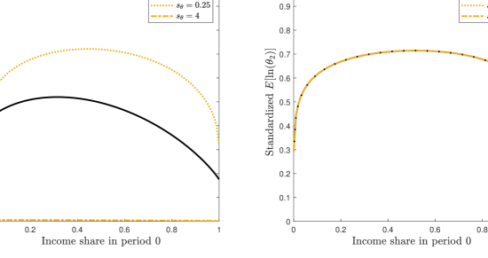
Figure 1: Mean response for different weights

3.2.4 Anchoring

Recall that we can write

$$\ln\tilde{\theta}_{t+1} = \tilde{a}_{t}+\tilde{\gamma}_{1t}\ln\tilde{\theta}_{t}+\tilde{\gamma}_{2t}\ln I_{t}+\tilde{\gamma}_{3t}\ln\tilde{\theta}_{t}\ln I_{t}+\tilde{\eta}_{\theta,t}$$

$$Z_{\theta,t,m} = \tilde{\mu}_{\theta,t,m}+\tilde{\lambda}_{\theta,t,m}\ln\tilde{\theta}_{t}+\varepsilon_{\theta,t,m}$$

$$Z_{I,t,m} = \tilde{\mu}_{I,t,m}+\tilde{\lambda}_{I,t,m}\ln\tilde{I}_{t}+{\varepsilon}_{I,t,m}\hskip 73.97716pt$$

$$\ln\tilde{I}_{t} = \tilde{\beta}_{0t}+\tilde{\beta}_{1t}\ln\tilde{\theta}_{t}+\tilde{\beta}_{2t}\ln Y_{t}+\tilde{\eta}_{I,t}$$

$$Q = \tilde{\rho}_{0}+\tilde{\rho}_{1}\ln\tilde{\theta}_{T}+\eta_{Q}$$

with $\tilde{\mu}_{\theta,t,0}=\tilde{\mu}_{I,t,0}=0$ and $\tilde{\lambda}_{\theta,t,0}=\tilde{\lambda}_{I,t,0}=1$, and the parameters in this system of equations are point identified by Theorem 1. Now define $\tilde{\vartheta}_{t}$ such that

$$\ln\tilde{\vartheta}_{t}=\tilde{\rho}_{0}+\tilde{\rho}_{1}\ln\tilde{\theta}_{t}.$$

We then get

$$\ln\tilde{\vartheta}_{t+1} = \tilde{\rho}_{0}+\tilde{\rho}_{1}\tilde{a}_{t}-\tilde{\rho}_{0}\tilde{\gamma}_{1t}+\tilde{\gamma}_{1t}\ln\tilde{\vartheta}_{t}+\tilde{\rho}_{1}\tilde{\gamma}_{2t}\ln I_{t}+\tilde{\gamma}_{3t}\ln\tilde{\vartheta}_{t}\ln I_{t}+\tilde{\rho}_{1}\tilde{\eta}_{\theta,t}$$

$$Z_{\theta,t,m} = \tilde{\mu}_{\theta,t,m}-\frac{\tilde{\rho}_{0}\tilde{\lambda}_{\theta,t,m}}{\tilde{\rho}_{1}}+\frac{\tilde{\lambda}_{\theta,t,m}}{\tilde{\rho}_{1}}\ln\tilde{\vartheta}_{t}+\varepsilon_{t}$$

$$Z_{I,t,m} = \tilde{\mu}_{I,t,m}+\tilde{\lambda}_{I,t,m}\ln\tilde{I}_{t}+{\varepsilon}_{I,t,m}\hskip 73.97716pt$$

$$\ln\tilde{I}_{t} = \tilde{\beta}_{0t}-\frac{\tilde{\rho}_{0}\tilde{\beta}_{1t}}{\tilde{\rho}_{1}}+\frac{\tilde{\beta}_{1t}}{\tilde{\rho}_{1}}\ln\tilde{\vartheta}_{t}+\tilde{\beta}_{2t}\ln Y_{t}+\tilde{\eta}_{I,t}$$

$$Q = \ln\tilde{\vartheta}_{T}+\eta_{Q}$$

CH:08 estimate a model for $\ln\tilde{\vartheta}_{t}$ which anchors the skills at the adult outcome. In particular, they first identify the model with $\ln\tilde{\theta}_{t}$ by using Assumptions 2 and 3(a). They then identify $\tilde{\rho}_{0}$ and $\tilde{\rho}_{1}$, redefine the skills as $\ln\tilde{\vartheta}_{t}$, and estimate the production function parameters. This strategy is equivalent to imposing the restrictions $\rho_{0}=0$ and $\rho_{1}=1$ instead of Assumption 2. Anchoring can help with the interpretation of certain parameters of the model. For example, when $E(Q\mid\ln\tilde{\vartheta}_{T})=\ln\tilde{\vartheta}_{T}$, then an increase of $\ln\tilde{\vartheta}_{T}$ by one corresponds to a one unit increase in the conditional expectation of $Q$. Moreover, the observed variable $Q$ can be used to study counterfactuals, such as income transfers, under Assumption 1 only, as shown in Theorem 2. However, as illustrated in Example 2, investment or income sequences that maximize the levels of the skills depend on the units of measurements of the anchor and are therefore hard to interpret. Instead on should focus on the log skill in which case such optimal sequences are invariant to the units of measurements.

As noted by CH:08, $\tilde{\gamma}_{1t}$ is invariant to the anchor. However, notice that Assumption 3(a) is an assumption and not a normalization with respect to $\gamma_{1t}$. Specifically, even with observed investment, $\tilde{\gamma}_{1t}$ is only equal to $\gamma_{1t}$ if $\lambda_{\theta,t,1}=\lambda_{\theta,t+1,1}$. The coefficient in front of investment is hard to interpreted because it depends on the specific anchor and its units of measurements (as also noted by CH:08). Moreover, notice that skills are anchored at the adult outcome, but investment is not, and many of the estimated parameters also depend on the units of the investment measures. While anchoring makes most sense under Assumption 3(a), in which case the skills in all periods are in the units of $Q$, we could instead use Assumption 3(b) to achieve point identification. In this case different adult outcomes or different units of measurements lead to different coefficients that possibly suggest very different dynamics, just as in Example 1.

3.2.5 Estimation

To estimate these features, one can use any existing estimator that relies on either Assumptions 1, 2, 3(a) and 4(a) or another set of identifying assumptions of Corollary 1. For example the estimator of AW:22 (if investment is exogenous) is computationally attractive. All of these sets of assumptions yield observationally equivalent models with potentially very different primitive parameters, but all features described in Theorem 2 will be identical. It is typically most convenient to set $\mu_{\theta,t,1}=\mu_{I,t,1}=0$ and $\lambda_{\theta,t,1}=\lambda_{I,t,1}=1$, estimate the implied primitive parameters, and then calculate the features in Theorem 2. AW:22 use Assumption 4(b) instead of 4(a) because they are concerned that their investment measures are not age-invariant. However, the restrictions in Assumption 4(b) are hard to interpret economically (in terms of constant returns to scale) because the parameters depend on the units of measurement of the data, as illustrated in Example 1. For the features described in Theorem 2, these assumptions are not required and the estimates do not depend on which set of assumptions is employed.

An alternative could be to use Assumption 1 only and an estimator that allows for partial identification. However, these methods can be computationally demanding with many parameters and seem to offer little benefits in this setting, because under Assumption 1 only, the identified sets are typically unbounded. Moreover, the features in Theorem 2 are point identified and can be recovered from an estimator in a point identified model.

3.3 CES production function

I now discuss the CES production technology where

(11) $$\theta_{t+1} = \left(\gamma_{1t}\theta_{t}^{\sigma_{t}}+\gamma_{2t}I_{t}^{\sigma_{t}}\right)^{\frac{\psi_{t}}{\sigma_{t}}}\exp(\eta_{\theta,t})\hskip 71.13188ptt=0,\ldots,T-1$$

(12) $$Z_{\theta,t,m} = \mu_{\theta,t,m}+\lambda_{\theta,t,m}\ln\theta_{t}+\varepsilon_{\theta,t,m}\hskip 76.82243ptt=0,\ldots,T,m=1,2$$

(13) $$Z_{I,t,m} = \mu_{I,t,m}+\lambda_{I,t,m}\ln I_{t}+\varepsilon_{I,t,m}\hskip 76.82243ptt=0,\ldots,T-1,m=1,2$$

(14) $$\ln I_{t} = \beta_{0t}+\beta_{1t}\ln\theta_{t}+\beta_{2t}\ln Y_{t}+\eta_{I,t}\hskip 59.75078ptt=0,\ldots,T-1$$

(15) $$Q = \rho_{0}+\rho_{1}\ln\theta_{T}+\eta_{Q}$$

In this case, it is also common that the measurement system is linear in $\ln\theta_{t}$, as in CHS:10 or AMN:19, to ensure that estimated skills are positive.

3.3.1 Identification

Similar to the trans-log case, define $\tilde{\theta}_{t}=\exp(\mu_{\theta,t,1})\theta_{t}^{\lambda_{\theta,t,1}}$ so that

$$\theta_{t}=\exp\left(-\frac{\mu_{\theta,t,1}}{\lambda_{\theta,t,1}}\right)\tilde{\theta}_{t}^{\frac{1}{\lambda_{\theta,t,1}}}.$$

Similarly, let $\tilde{I}_{t}=\exp(\mu_{I,t,1})I_{t}^{\lambda_{I,t,1}}$. We can then rewrite the production technology in terms of $\tilde{\theta}_{t}$ and $\tilde{I}_{t}$. That is, we can rewrite equations (11)–(15) to

(16) $$\tilde{\theta}_{t+1} = \left(\tilde{\gamma}_{1t}\tilde{\theta}_{t}^{\frac{\sigma_{t}}{\lambda_{\theta,t,1}}}+\tilde{\gamma}_{2t}\tilde{I}_{t}^{\frac{\sigma_{t}}{\lambda_{I,t,1}}}\right)^{\frac{\lambda_{\theta,t+1,1}\psi_{t}}{\sigma_{t}}}\exp(\tilde{\eta}_{\theta,t})\hskip 36.98857ptt=0,\ldots,T-1$$

(17) $$Z_{\theta,t,m} = \tilde{\mu}_{\theta,t,m}+\tilde{\lambda}_{\theta,t,m}\ln\tilde{\theta}_{t}+\varepsilon_{\theta,t,m}\hskip 108.12047ptt=0,\ldots,T,m=1,2$$

(18) $$\hskip 34.1433ptZ_{I,t,m} = \tilde{\mu}_{I,t,m}+\tilde{\lambda}_{I,t,m}\ln\tilde{I}_{t}+{\varepsilon}_{I,t,m}\hskip 108.12047ptt=0,\ldots,T-1,m=1,2$$

(19) $$\ln\tilde{I}_{t} = \tilde{\beta}_{0t}+\tilde{\beta}_{1t}\ln\tilde{\theta}_{t}+\tilde{\beta}_{2t}\ln Y_{t}+\tilde{\eta}_{I,t}\hskip 91.04881ptt=0,\ldots,T-1$$

(20) $$Q = \tilde{\rho}_{0}+\tilde{\rho}_{1}\ln\tilde{\theta}_{T}+\eta_{Q}$$

where

$$\tilde{\gamma}_{1t}=\gamma_{1t}\exp\left(\sigma_{t}\left(\frac{\mu_{\theta,t+1,1}}{\lambda_{\theta,t+1,1}}-\frac{\mu_{\theta,t,1}}{\lambda_{\theta,t,1}}\right)\right)\quad\text{and}\quad\tilde{\gamma}_{2t}=\gamma_{2t}\exp\left(\sigma_{t}\left(\frac{\mu_{\theta,t+1,1}}{\lambda_{\theta,t+1,1}}-\frac{\mu_{I,t,1}}{\lambda_{I,t,1}}\right)\right)$$

and the other parameters are defined as in the trans-log case. The following theorem characterizes the identified set of the finite dimensional parameters.

Theorem 3.

Suppose Assumption 1 holds.

1. The identified set of $\{\mu_{\theta,t,m},\lambda_{\theta,t,m}\}_{t=0,\ldots,T,m=1,2}$, $\{\mu_{I,t,m},\lambda_{I,t,m}\}_{t=0,\ldots,T-1,m=1,2}$, $(\rho_{0},\rho_{1})$, $\{\beta_{0t},\beta_{1t},\beta_{2t}\}^{T-1}_{t=0}$, $\{\gamma_{1t},\gamma_{2t},\sigma_{t},\psi_{t}\}^{T-1}_{t=0}$ consists of all vectors that yield the same values of $\{\tilde{\mu}_{\theta,t,m},\tilde{\lambda}_{\theta,t,m}\}_{t=0,\ldots,T,m=1,2}$, $\{\tilde{\mu}_{I,t,m},\tilde{\lambda}_{I,t,m}\}_{t=0,\ldots,T-1,m=1,2}$, $(\tilde{\rho}_{0},\tilde{\rho}_{1})$, $\{\tilde{\gamma}_{1t},\tilde{\gamma}_{2t},\frac{\sigma_{t}}{\lambda_{\theta,t,1}},\frac{\sigma_{t}}{\lambda_{I,t,1}}\}^{T-1}_{t=0}$, $\{\frac{\sigma_{t}\psi_{t}}{\lambda_{\theta,t+1,1}}\}^{T-1}_{t=0}$, and $\{\tilde{\beta}_{0t},\tilde{\beta}_{1t},\tilde{\beta}_{2t}\}^{T-1}_{t=0}$ as the true parameter vectors.

2. Let $\{\bar{\mu}_{\theta,t,1}\}_{t=0}^{T}$, $\{\bar{\mu}_{I,t,1}\}_{t=0}^{T-1}$, and $\{\bar{\lambda}_{\theta,t,1}\}_{t=0}^{T}$ be fixed constants with $\bar{\lambda}_{\theta,t,1}\neq 0$ for all $t$. Under the additional restrictions $\{{\mu}_{\theta,t,1}\}_{t=0}^{T}=\{\bar{\mu}_{\theta,t,1}\}_{t=0}^{T}$ and $\{{\mu}_{I,t,1}\}_{t=0}^{T-1}=\{\bar{\mu}_{I,t,1}\}_{t=0}^{T-1}$ and $\{{\lambda}_{\theta,t,1}\}_{t=0}^{T}=\{\bar{\mu}_{\theta,t,1}\}_{t=0}^{T}$ the identified set is a singleton.

An important implications of part (a) is that the fraction $\frac{\lambda_{\theta,t,1}}{\lambda_{I,t,1}}=\frac{\lambda_{\theta,t,1}}{\sigma_{t}}\frac{\sigma_{t}}{\lambda_{I,t,1}}$ is point identified for all $t=1,\ldots,T-1$. Hence, if we restrict $\lambda_{\theta,t,1}$ to a constant, $\lambda_{I,t,1}$ is identified, which is very different to the trans-log case. Intuitively, since skills and investment have the same exponent in the CES production functions, the relative scale is identified by the functional form restrictions.

As before, I now introduce additional assumptions to achieve point identification.

Assumption 2’.

$\lambda_{\theta,0,1}=1$ and $\mu_{\theta,0,1}=0$.

Assumption 3’.

1. $\mu_{\theta,t,1}=\mu_{\theta,t+1,1}$ for all $t=0,\ldots,T-1$

2. $\gamma_{1t}+\gamma_{2t}=1$ for all $t=0,\ldots,T-1$.

Assumption 4’.

1. $\mu_{I,t,1}=\mu_{I,t+1,1}=0$ for all $t=0,\ldots,T-2$.

2. $\beta_{0t}=0$ for all $t=0,\ldots,T-1$.

Assumption 5’.

1. $\lambda_{\theta,t,1}=\lambda_{\theta,t+1,1}$ for all $t=0,\ldots,T-1$.

2. $\psi_{t}=1$ for all $t=0,\ldots,T-1$.

The following result shows how point identification can be established.

Corollary 2.

Suppose Assumptions 1 and 2’ hold. Suppose either Assumption 3’(a) or Assumption 3’(b) holds. Suppose either Assumption 4’(a) or Assumption 4’(b) holds. Suppose either Assumption 5’(a) or Assumption 5’(b) holds. Then all parameters are point identified.

A common restriction with the CES production function is to set $\psi_{t}=1$ for all $t$ (see e.g. CHS:10 and AMN:19). In this case, Theorem 3 implies that $\frac{\lambda_{\theta,t+1,1}}{\lambda_{\theta,t,1}}$ is point identified. Hence, assuming age-invariance (i.e. $\frac{\lambda_{\theta,t+1,1}}{\lambda_{\theta,t,1}}=1$) is not required, and it is in fact a testable implication. Moreover, with this additional restriction, Corollary 2 implies that the only scale restriction needed is $\lambda_{\theta,0,1}=0$. Nevertheless, it is common practice to set ${\lambda}_{\theta,t,1}={\lambda}_{I,t,1}=1$ for all $t$, which are not normalizations, but in fact very restrictive assumptions (even if $\psi_{t}\neq 1$). Setting the scales to different numbers or changing the units of measurement of the data then affects all estimated parameters, optimal investment sequences, and other counterfactuals. The exact consequences depend on the estimation methods used. As an illustration I consider the estimator of AMN:19 in Section 3.4.

Again, these sets of assumptions are not only sufficient, but also necessary for point identification. In particular, as shown in Theorem 7 in the appendix and illustrated in examples below, if the model is correctly specified and Assumption 1 holds, then there always exist sets of parameters which are consistent with the data and satisfy Assumptions 1, 2’, either 3’(a) or 3’(b), and either 4’(a) or 4’(b), and either 5’(a) or 5’(b). Again, different sets of assumptions yield observationally equivalent models, but potentially very different primitive parameters.

Remark 3.

There is also a large macroeconomic literature on normalized CES production functions; see for example KG:00, KMW:12, Temple:12 and references therein. They note that one can always write

$$\left(\gamma_{1t}\theta_{t}^{\sigma_{t}}+\gamma_{2t}I_{t}^{\sigma_{t}}\right)^{\frac{1}{\sigma_{t}}}=\bar{A}_{t}\left(\bar{\gamma}_{t}\left(\frac{\theta_{t}}{\bar{\theta}_{t}}\right)^{\sigma_{t}}+(1-\bar{\gamma}_{t})\left(\frac{I_{t}}{\bar{I}_{t}}\right)^{\sigma_{t}}\right)^{\frac{1}{\sigma_{t}}}$$

where $\bar{\theta}_{t}$ and $\bar{I}_{t}$ are fixed constants to be chosen by the researcher to standardize the inputs,

$$\bar{\gamma}_{t}=\frac{\gamma_{1t}\bar{\theta}_{t}^{\sigma_{t}}}{\gamma_{1t}\bar{\theta}_{t}^{\sigma_{t}}+\gamma_{2t}\bar{I}_{t}^{\sigma_{t}}}\quad\text{ and }\quad\bar{A}_{t}=\left(\gamma_{1t}\bar{\theta}_{t}^{\sigma_{t}}+\gamma_{2t}\bar{I}_{t}^{\sigma_{t}}\right)^{\frac{1}{\sigma_{t}}}.$$

Estimating the production function with these two different specifications yields observationally equivalent models with the same elasticity of substitution. By standardizing the inputs, we can evaluate the production function at $\theta_{t}=\bar{\theta}_{t}$ and $I_{t}=\bar{I}_{t}$ to get the output $\bar{A}_{t}$. If the units of measurements of the inputs are known, such standardizations can help interpret the parameters and calibrate the model, while without an implicit normalization $\gamma_{1t}$ and $\gamma_{2t}$ are harder to interpret. Moreover, the consequences of changing $\sigma_{t}$, while holding the other parameters fixed, on functions of interest might depends on how the model is parameterized because $\bar{\gamma}_{t}$ and $\bar{A}_{t}$ depend on $\sigma_{t}$.

One potential choice of standardizations could be $\bar{\theta}_{t}=E[\theta_{t}]$ and $\bar{I}_{t}=E[I_{t}]$ (see Embrey:19 for this standardization). However, since the inputs are not observed, $E[\theta_{t}]$ and $E[I_{t}]$ are not identified. Instead, we can write

$$\theta_{t+1}=\bar{A}_{t}\left(\bar{\gamma}_{t}\left(\frac{\theta_{t}}{E[\theta_{t}]}\right)^{\sigma_{t}}+(1-\bar{\gamma}_{t})\left(\frac{I_{t}}{E[{I}_{t}]}\right)^{\sigma_{t}}\right)^{\frac{1}{\sigma_{t}}}\exp(\eta_{\theta,t})$$

as

$$\tilde{\theta}_{t+1} =\exp(\mu_{\theta,t+1,1})\bar{A}_{t}\left(\bar{\gamma}_{t}\left(\frac{\tilde{\theta}_{t}}{E[\tilde{\theta}_{t}^{1/\lambda_{\theta,t,1}}]^{\lambda_{\theta,t,1}}}\right)^{\frac{\sigma_{t}}{\lambda_{\theta,t,1}}}+(1-\bar{\gamma}_{t})\left(\frac{\tilde{I}_{t}}{E[\tilde{I}_{t}^{1/\lambda_{I,t,1}}]^{\lambda_{I,t,1}}}\right)^{\frac{\sigma_{t}}{\lambda_{I,t,1}}}\right)^{\frac{\lambda_{\theta,t+1,1}\psi_{t}}{\sigma_{t}}}\exp(\tilde{\eta}_{\theta,t})$$

To achieve the desired standardization, we would have to standardize the inputs in equation (16) by $E[\tilde{\theta}_{t}^{1/\lambda_{\theta,t,1}}]^{\lambda_{\theta,t,1}}$ and $E[\tilde{I}_{t}^{1/\lambda_{I,t,1}}]^{\lambda_{I,t,1}}$, respectively, which are not identified. We could instead standardize by $E[\tilde{\theta}_{t}]$ and $E[\tilde{I}_{t}]$, but is not clear if such a standardization would yield a useful interpretation of the parameters. Finally, notice that the most important issue with the current specification of the CES production function is overidentification and biased estimators due to setting the scales, which is not mitigated by standardizing inputs.

3.3.2 Invariant parameters

As in the trans-log case, important policy relevant parameters are point identified under Assumption 1 only. The interpretation of these features has been discussed in Section 3.2.2.

Theorem 4.

Suppose Assumption 1 holds.

1. $F_{\theta_{t+1}}\left(\left(\gamma_{1t}Q_{\alpha_{1}}(\theta_{t})^{\sigma_{t}}+\gamma_{2t}Q_{\alpha_{2}}(I_{t})^{\sigma_{t}}\right)^{\frac{\psi_{t}}{\sigma_{t}}}\exp(Q_{\alpha_{3}}(\eta_{\theta,t}))\right)$ is point identified for all $\alpha_{1},\alpha_{2},\alpha_{3}\in(0,1)$

2. Let

   $$\ln I_{t}(Y)=\beta_{0t}+\beta_{1t}\ln Q_{\alpha_{1}}(\theta_{t})+\beta_{2t}\ln Y+Q_{\alpha_{4}}(\eta_{I,t})$$

   Then

   $$F_{\theta_{t+1}}\left(\left(\gamma_{1t}Q_{\alpha_{1}}(\theta_{t})^{\sigma_{t}}+\gamma_{2t}I_{t}(Y)^{\sigma_{t}}\right)^{\frac{1}{\sigma_{t}}}\exp(Q_{\alpha_{3}}(\eta_{\theta,t}))\right)$$

   is point identified for all $\alpha_{1},\alpha_{3},\alpha_{4}\in(0,1)$.

3. $P\left(Q\leq q\mid\theta_{t}=Q_{\alpha_{1}}(\theta_{t}),\{I_{s}=Q_{\alpha_{2s}}(I_{s})\}^{T-1}_{s=t},\{\eta_{\theta,s}=Q_{\alpha_{3s}}(\eta_{\theta,s})\}^{T-1}_{s=t}\right)$ is point identified for all $\alpha_{1},\{\alpha_{2s},\alpha_{3s}\}^{T-1}_{s=t}\in(0,1)$.

4. $P\left(Q\leq q\mid\theta_{0}=Q_{\alpha}(\theta_{0}),\{Y_{t}=y_{t}\}^{T-1}_{t=0}\right)$ is point identified for all $\alpha\in(0,1)$.

5. If in addition either Assumption 5’(a) or Assumption 5’(b) holds, then the distributions of

   $$\frac{\partial\ln\theta_{t+1}}{\partial\ln\theta_{t}}=\frac{\partial}{\partial\ln\theta_{t}}\ln\left(\gamma_{1t}\theta_{t}^{\sigma_{t}}+\gamma_{2t}I_{t}^{\sigma_{t}}\right)^{\frac{1}{\sigma_{t}}}$$

   and

   $$\frac{\partial\ln\theta_{t+1}}{\partial\ln I_{t}}=\frac{\partial}{\partial\ln I_{t}}\ln\left(\gamma_{1t}\theta_{t}^{\sigma_{t}}+\gamma_{2t}I_{t}^{\sigma_{t}}\right)^{\frac{1}{\sigma_{t}}}$$

   are point identified and

   $$\left.\frac{\partial\ln\theta_{t+1}}{\partial\ln\theta_{t}}\right|_{\ln\theta_{t}=Q_{\alpha_{1}}(\ln\theta_{t}),\ln I_{t}=Q_{\alpha_{2}}(\ln I_{t})}=\left.\frac{\partial}{\partial\ln\theta_{t}}\ln\left(\gamma_{1t}\theta_{t}^{\sigma_{t}}+\gamma_{2t}I_{t}^{\sigma_{t}}\right)^{\frac{1}{\sigma_{t}}}\right|_{\ln\theta_{t}=Q_{\alpha_{1}}(\ln\theta_{t}),\ln I_{t}=Q_{\alpha_{2}}(\ln I_{t})}$$

   and

   $$\left.\frac{\partial\ln\theta_{t+1}}{\partial\ln I_{t}}\right|_{\ln\theta_{t}=Q_{\alpha_{1}}(\ln\theta_{t}),\ln I_{t}=Q_{\alpha_{2}}(\ln I_{t})}=\left.\frac{\partial}{\partial\ln I_{t}}\ln\left(\gamma_{1t}\theta_{t}^{\sigma_{t}}+\gamma_{2t}I_{t}^{\sigma_{t}}\right)^{\frac{1}{\sigma_{t}}}\right|_{\ln\theta_{t}=Q_{\alpha_{1}}(\ln\theta_{t}),\ln I_{t}=Q_{\alpha_{2}}(\ln I_{t})}$$

   are point identified for all $\alpha_{1},\alpha_{2}\in(0,1)$.

The features in parts (1)–(4) are analogous to those in the trans-log case and can be used to calculate optimal investment/income strategies and anchored treatment effects, as discussed after Theorem 2. As opposed to the trans-log case, now the relative scales of skills and investment are point identified. Consequently, elasticities are identified under Assumption 1 and either age-invariant skill measures or $\psi_{t}=1$ only.

3.3.3 Non-invariant parameters

To achieve point identification of all parameters, we need to fix the levels of the log skills and investment, for example by setting $\mu_{\theta,0,1}$ and $\mu_{0,I,1}$ to $0$. I now discuss whether these restrictions are normalizations with respect to any of the primitive parameters. Again, I assume that investment is observed and focus on the location of the skills. Notice that with the age-invariance assumption $\mu_{\theta,t,1}=\mu_{\theta,t+1,1}$, Theorem 3 implies that $\mu_{\theta,0,1}=0$ is in general not a normalization with respect to $\gamma_{1t}$ and $\gamma_{2t}$. An exception is the special case where $\lambda_{\theta,t,1}=\lambda_{\theta,t+1,1}$. Then $\mu_{\theta,0,1}=0$ is a normalization with respect to $\gamma_{1t}$, but not $\gamma_{2t}$.

Next, consider the restriction $\gamma_{1t}+\gamma_{2t}=1$. In this case $\mu_{\theta,0,1}=0$ is in general not a normalization with respect to $\gamma_{1t}$ or $\gamma_{2t}$ and different scales can lead to very different dynamics, which I illustrate in the example below. Here $\mu_{\theta,0,1}$ (and not $\lambda_{\theta,0,1}$) affects the scale because we can identify the distribution of $\tilde{\theta}_{\theta,t,1}=\exp(\mu_{\theta,t,1})\theta_{t}^{\lambda_{\theta,t,1}}$ and the production function is in levels rather than logs of $\theta_{t}$.

Example 3.

The issues with the restriction $\mu_{\theta,0,1}=0$ in the CES case are analogous to the issues with the restriction $\lambda_{\theta,0,1}=1$ in the trans-log case discussed in Example 1. I now consider a numerical example analogous to Example 1 and focus on the measurement and the production function only. That is, suppose that

$$\theta_{t+1} = \left(\frac{1}{2}\theta_{t}+\frac{1}{2}I_{t}\right)\exp(\eta_{\theta,t})$$

$$Z_{\theta,t,m} = \ln(12)+\ln\theta_{t}+\varepsilon_{\theta,t,m}$$

Hence, $\gamma_{1t}$ and $\gamma_{2t}$ sum to $1$, they are identical and they do not change over time. Moreover, $\lambda_{\theta,t,m}=\sigma_{t}=1$ for all $t$. Notice that

$$Z_{\theta,t,m}=\ln(12\theta_{t})+\varepsilon_{\theta,t,m}.$$

Let $\tilde{\theta}_{t}=12\theta_{t}$. Just as in Example 1, we get

$$\tilde{\theta}_{t+1} = \left(\tilde{\gamma}_{1t}\tilde{\theta}_{t}+(1-\tilde{\gamma}_{1t})I_{t}\right)\exp(\tilde{\eta}_{\theta,t})$$

$$Z_{\theta,t,m} = \tilde{\mu}_{\theta,t,m}+\ln\tilde{\theta}_{t}+\varepsilon_{\theta,t,m}$$

where

$$(\tilde{\gamma}_{10},\tilde{\gamma}_{11},\tilde{\gamma}_{12},\tilde{\gamma}_{13},\ldots)=(0.077,0.351,0.435,0.470,\ldots)$$

and

$$(\exp(\tilde{\mu}_{0,\theta,m}),\exp(\tilde{\mu}_{1,\theta,m}),\exp(\tilde{\mu}_{2,\theta,m}),\exp(\tilde{\mu}_{3,\theta,m}),\ldots)=(1,6.5,9.25,10.625,\ldots).$$

These two models are observationally equivalent, but the two sets of parameters might suggest very different dynamics.

3.3.4 Anchoring

Again we can write the measurement system and the adult outcome as

$$Z_{\theta,t,m} = \tilde{\mu}_{\theta,t,m}-\frac{\tilde{\rho}_{0}\tilde{\lambda}_{\theta,t,m}}{\tilde{\rho}_{1}}+\frac{\tilde{\lambda}_{\theta,t,m}}{\tilde{\rho}_{1}}\ln\tilde{\vartheta}_{t}+\varepsilon_{t}$$

$$Q = \ln\tilde{\vartheta}_{T}+\eta_{Q}$$

where the joint distribution of $\{\ln\tilde{\vartheta}_{t}\}^{T}_{t=1}$ and $\tilde{\rho}_{0}$ and $\tilde{\rho}_{1}$ are point identified. In general, the implications of anchoring are similar to those in the trans-log case and it replaces Assumption 2’. However, recall that the relative scale of investment and skills is identified and we therefore cannot anchor both variables to a measure or adult outcome. Moreover, if investment was observed and either Assumption 5’(a) or Assumption 5’(b) holds, then $\{\lambda_{\theta,t,1}\}^{T}_{t=0}$ is point identified and the model can only be consistent with one particular (identified) scale of the skills. Thus, we can only have a CES production technology for $\{\tilde{\vartheta}_{t}\}^{T}_{t=0}$ if $\alpha_{1}=1$ and the model cannot be consistent with different anchors or different units of measurement.

3.3.5 Estimation

As in the trans-log case, we can estimate the model using any combinations of assumptions in Corollary 2 that yield point identification. No matter which combination is used, estimates of the features in Theorem 3, including elasticities when $\psi_{t}=1$, will be identical. In this section I outline one particular way to do so based on equations (16)–(20) together with Assumptions 1, 2’, 3’(a), and 4’(a), and 5’(b) and an adaptation of the estimation approach of AMN:19.

In the first step, we can use the restriction $\tilde{\lambda}_{\theta,t,1}=\tilde{\lambda}_{I,t,1}=1$ for all $t$ and $\tilde{\mu}_{\theta,t,m}=\tilde{\mu}_{I,t,m}=0$ for all $t$ and $m$ to estimate the joint distribution of $(\{\tilde{\theta}_{t}\}^{T}_{t=0},\{\tilde{I}_{t},Y_{t}\}^{T}_{t=0},Q)$ as well as $\tilde{\lambda}_{\theta,t,m}$, $\tilde{\lambda}_{I,t,m}$ for all $t$ and $m>1$, $\tilde{\rho}_{0}$, and $\tilde{\rho}_{1}$. For example, AMN:19 assume that the measures, log-skills, and log-investment, log-income, have a normal mixture distribution. In the second step, we can take draws from the estimated joint distribution and estimate the remaining parameters. To do so, let $\{\{\tilde{\theta}_{t,j}\}^{T}_{t=0},\{\tilde{I}_{t,j},Y_{t,j}\}^{T}_{t=0},Q_{j}\}^{J}_{j=1}$ be these draws and let

$$(\hat{\tilde{\beta}}_{0t},\hat{\tilde{\beta}}_{1t},\hat{\tilde{\beta}}_{2t})=\operatorname*{arg\,min}_{\{\tilde{\beta}_{0t},\tilde{\beta}_{1t},\tilde{\beta}_{2t}\}}\sum^{J}_{j=1}\left(\ln\tilde{I}_{t,j}-\tilde{\beta}_{0t}-\tilde{\beta}_{1t}\ln\tilde{\theta}_{t,j}-\tilde{\beta}_{2t}\ln Y_{t,j}\right)^{2}$$

and $\hat{\tilde{\eta}}_{I,t,j}=\ln\tilde{I}_{t,j}-\hat{\tilde{\beta}}_{0t}-\hat{\tilde{\beta}}_{1t}\ln\tilde{\theta}_{t,j}-\hat{\tilde{\beta}}_{2t}\ln Y_{t,j}$. Next set $\hat{\lambda}_{\theta,0,1}={\lambda}_{\theta,0,1}=1$ and let

$$(\{\hat{\lambda}_{\theta,t,1}\}^{T-1}_{t=1},\{\hat{\lambda}_{I,t,1},\hat{\sigma}_{t},\hat{\gamma}_{1t},\hat{\gamma}_{2t},\hat{\tilde{\kappa}}_{t}\}^{T-1}_{t=0})$$

$$=\operatorname*{arg\,min}_{\{\lambda_{\theta,t,1}\}^{T-1}_{t=1},\{\lambda_{I,t,1},\sigma_{t},{\gamma}_{1t},{\gamma}_{2t},\tilde{\kappa}_{t}\}^{T-1}_{t=0}}\sum^{T}_{t=1}\sum^{J}_{j=1}\left(\ln\tilde{\theta}_{t+1,j}-{\frac{\lambda_{\theta,t+1,1}}{\sigma_{t}}}\ln\left({\gamma}_{1t}\tilde{\theta}_{t,j}^{\frac{\sigma_{t}}{\lambda_{\theta,t,1}}}+{\gamma}_{2t}\tilde{I}_{t,j}^{\frac{\sigma_{t}}{\lambda_{I,t,1}}}\right)-\tilde{\kappa}_{t}\hat{\tilde{\eta}}_{I,t,j}\right)^{2}$$

Using these estimates, we can the recover $\hat{\lambda}_{\theta,t,m}=\hat{\tilde{\lambda}}_{\theta,t,m}\hat{\lambda}_{\theta,t,1}$, $\hat{\lambda}_{I,t,m}=\hat{\tilde{\lambda}}_{I,t,m}\hat{\lambda}_{I,t,1}$, $\hat{\beta}_{0t}=\frac{\tilde{\beta}_{0t}}{\hat{\lambda}_{I,t,1}}$, $\hat{\rho}_{0}=\hat{\tilde{\rho}}_{0}$, $\hat{\rho}_{1}=\hat{\tilde{\rho}}_{1}\hat{\lambda}_{\theta,t,1}$, $\hat{\beta}_{1t}=\tilde{\beta}_{1t}\frac{\hat{\lambda}_{\theta,t,1}}{\hat{\lambda}_{I,t,1}}$, and $\hat{\beta}_{2t}=\frac{\tilde{\beta}_{2t}}{\hat{\lambda}_{I,t,1}}$, as well as the estimated distributions of skills and investment using the relationship $\ln\theta_{t}=\frac{\ln\tilde{\theta}_{t}}{{\lambda}_{\theta,t,1}}$ and $\ln I_{t}=\frac{\ln\tilde{I}_{t}}{{\lambda}_{I,t,1}}$. The estimation procedure also easily allows imposing additional assumptions, such as age-invariance of the first skill measure in which case ${\lambda}_{\theta,1,1}={\lambda}_{\theta,t,1}$ for all $t$.

The parameter estimates generally depend on the scale and location restrictions imposed and are therefore are very hard to interpret. However, using these estimates, we can calculate the features in Theorem 3, which are invariant to the restrictions.

3.4 Monte Carlo simulations

I use a very similar data generating process as AMN:19. In particular, I use

$$\theta_{t+1}=A_{t}\left(\gamma_{t}\theta_{t}^{\sigma_{t}}+\left(1-\gamma_{t}\right)I_{t}^{\sigma_{t}}\right)^{\frac{1}{\sigma_{t}}}\exp(\eta_{\theta,t})$$

for $t=1,2$. Allowing for $A_{t}\neq 1$ is equivalent to not imposing the restriction that the coefficients in front of $\theta_{t}$ and $I_{t}$ sum to $1$. Since I want to study income transfers as counterfactuals, I augment the setup of AMN:19 and add the equation

$$\ln I_{t}=\beta_{1t}\ln\theta_{t}+\beta_{2t}\ln Y_{t}+\eta_{I,t}$$

where $Y_{t}$ is the same in all periods. To simulate data, I first draw $(\ln(\theta_{0}),\ln(Y))$ from a normal mixture distribution. Given $(\ln(\theta_{0}),\ln(Y))$ and normally distributed $\eta_{\theta,t}$ and $\eta_{I,t}$ I then generate $I_{0}$, $\theta_{1}$, $I_{1}$, and $\theta_{2}$ using the model. If $\ln I_{t}$ was equal to $\ln Y_{t}$, the setup would be exactly equal to that of AMN:19 with parameters as in their Table 9, which are based on their empirical results, and I use $\sigma_{0}=\sigma_{1}=-0.5$. I deviate slightly from their setting by using the additional investment equation with $\beta_{1t}=0.1$, $\beta_{2t}=0.9$, and $\eta_{I,t}\sim N(0,0.1^{2})$. I simulate three measures each for $\theta_{t}$ and $I_{t}$, which have a factor structure with $\mu_{t,\theta,m}=\mu_{t,I,m}=0$ for all $m,t$. In addition $\lambda_{t,\theta,1}=\lambda_{t,I,1}=1$ for all $t$, which imposes the scale restrictions and the age-invariance assumptions. These loadings are then also “normalized” to $1$ in the estimation procedure. Specifically, following AMN:19 I first estimate the distribution of the measures and of log-income using a normal mixture model. Then, assuming that $(\ln(\theta_{0}),\ln(\theta_{1}),\ln(\theta_{2}),\ln(I_{0}),\ln(I_{1}),\ln(Y))$ also has a normal mixture distribution, one can use the factor structure and the restrictions to estimate that joint distribution. Once we have the estimated joint distribution of $(\ln(\theta_{0}),\ln(\theta_{1}),\ln(\theta_{2}),\ln(I_{0}),\ln(I_{1}),\ln(Y))$, we can draw a sample from that distribution and estimate all production function parameters by nonlinear least squares.

I use the estimation procedure explained in Section 3.3.5, which simplifies in this setup because investment is exogenous (and thus, $\kappa_{t}=0$). Moreover, to focus on the scale restriction only, I set $\mu_{\theta,t,m}=\mu_{I,t,m}=0$ for all $m$ and $t$. Finally, I impose that the first skill measures is age-invariant, set $\lambda_{\theta,t,1}=1$ for all $t$, and estimate $\lambda_{I,t,1}$. I therefore impose Assumptions 2’, 3’(a), and 4’(a), as well as both parts of Assumption 5’. While only one part of the last assumption is needed (i.e. age-invariance of the skill measures could be dropped), they are both satisfied in this setup. That is, I estimate $\lambda_{I,t,1}$ along with the production function parameters by solving

$$(\hat{\lambda}_{I,t,1},\hat{\sigma}_{1},\hat{\sigma}_{2},\hat{\gamma}_{11},\hat{\gamma}_{21},\hat{\gamma}_{11},\hat{\gamma}_{21})$$

$$\qquad\qquad=\operatorname*{arg\,min}_{{\lambda}_{I,1},{\sigma}_{1},{\sigma}_{2},{\gamma}_{11},{\gamma}_{21},{\gamma}_{11},{\gamma}_{21}}\sum^{T}_{t=1}\sum^{J}_{j=1}\left(\ln\tilde{\theta}_{t+1,j}-{\frac{1}{\sigma_{t}}}\ln\left({\gamma}_{1t}\tilde{\theta}_{t,j}^{\sigma_{t}}+{\gamma}_{2t}\tilde{I}_{t,j}^{\frac{\sigma_{t}}{\lambda_{I,t,1}}}\right)\right)^{2}$$

where $\tilde{\theta}_{t,j}$ and $\tilde{I}_{t,j}$ are draws from the estimated distribution. Similarly, we can estimate $\beta_{1t}$ and $\beta_{2t}$ from a regression of $\tilde{I}_{t,j}$ on $\tilde{\theta}_{t,j}$ and $Y_{j}$. In addition, I use the estimator of AMN:19, which also imposes the overidentifying restriction $\lambda_{I,t,1}=1$ for all $t$.

In the following, I will investigate the effect of multiplying the skill measures by a single constant $s_{\theta}$ in all periods, which changes the loadings, but not the age-invariance assumption. For example, the first measure, say $\tilde{Z}_{\theta,t,1}$, is generated by

$$\tilde{Z}_{\theta,t,1}=\log(\theta_{t})+\varepsilon_{\theta,t,1}$$

but when I estimate the model, I use

$$Z_{\theta,t,1}=s_{\theta}\tilde{Z}_{\theta,t,1}=s_{\theta}\log(\theta_{t})+s_{\theta}\varepsilon_{\theta,t,1},$$

which is also an age-invariant measure. The estimators still impose that the loadings are equal to 1 ($\lambda_{\theta,t,1}=1$ for all $t$ with my estimator and $\lambda_{\theta,t,1}=1$ and $\lambda_{I,t,1}=1$ for all $t$ with the estimator of AMN:19). Of course, in practice, we do not know the DGP and there is no reason to believe that the true loading is $1$. Ideally, the restriction should be a normalization in which case the results would be invariant to scaling the data or changing its units of measurement. However, Corollary 2 implies that the estimator of AMN:19 is inconsistent. I look at the implications for elasticities and counterfactual predictions, which are point identified (as shown in Theorem 4) and are invariant to the scaling when using the new estimator. I take $s_{\theta}=1$, which is the correctly specified model, as well as $s_{\theta}=2/3$ and $s_{\theta}=2$, which are small changes of the units of measurement that have a large impact on the results. I report average estimates from 200 simulated data sets.

To summarize the production function estimates I report ${\partial\ln(\theta_{1})}/{\partial\ln(\theta_{0})}$ as a function of quantiles of $\ln(\theta_{0})$ and evaluated at the median value of $I_{0}$ and ${\partial\ln(\theta_{2})}/{\partial\ln(I_{1})}$ as a function of quantiles of $\ln(I_{1})$ and evaluated at the median value of $\theta_{1}$, which are point identified, as shown in the last part of Theorem 4. Figure 2 shows these partial derivatives for the true parameters, the 2-step estimator of AMN:19 with different values of $s_{\theta}$, and the invariant estimator that also estimates the scale. In this and the following figures, the results obtained with the invariant estimator are always almost identical to those with the 2-step estimator and $s_{\theta}=1$ and very similar to those with the true parameter values. However, the figure also demonstrates that small changes in the units of measurements can have a large effect on the results when using the 2-step estimator. The invariant estimator, on the other hand, can adapt to the scale change and yields identical results for the reported features (but not the parameter estimates) no matter what the scale is. One interesting finding is that the 2-step estimator underestimates the partial derivative with respect to $\ln(\theta_{0})$ for small values of the inputs and overestimates it for large values when $s_{\theta}=2/3$.

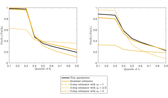
Figure 2: Partial derivatives

As a first counterfactual, consider an individual, whose value of $\theta_{0}$ equals $Q_{0.1}(\theta_{0})$ and all unobservables are $0$. I then exogenously change the income sequence of that individual and check the implied quantile in the skill distribution in period $2$. Of course, the larger income, the higher the relative rank/quantile in the last period. I report results where a feasible choice of income in each period is a given quantile (that will be varied). Instead of using the feasible choices, I distribute the total income among the two periods to maximize the skill quantile in the last period. The second part of Theorem 4 implies that these counterfactuals are point identified, can be consistently estimated with the invariant estimator, but the results with the 2-step estimator of AMN:19 will depend on $s_{\theta}$.

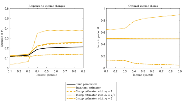
Figure 3: Response to income changes and optimal shares

The left panel of Figure 3 shows the quantile as a function of the feasible income quantile ($0.5$ is the median, etc.). Using the true parameters, we can see that, even for large income, the quantile in period $2$ is at most around $0.22$ and does not go much below the initial value of $0.1$ for low income. The right panel of Figure 3 shows the corresponding optimal income shares in period $0$. With the true parameters, income should be similar in both periods. The 2-step estimator with $s_{\theta}=1$ and the invariant estimator (irrespective of the scale) yield almost identical conclusions for the optimal income sequence, but have a small bias for the estimated quantile in period $2$ (due the approximation error of the joint distribution of the measures/skills as mixtures of normals).

Figure 3 also demonstrates that changing the units of measurement can lead to inefficient income transfers when using the 2-step estimator. For example, with $s_{\theta}=2/3$ the results suggest that we should mainly invest at $t=0$, and with $s_{\theta}=2$ it appears that we should mainly invest at $t=1$. Moreover, the estimated gains of income transfers are misleading in this case. As can be seen from the left panel, the inconsistent estimates suggest that large income transfers can increase the quantile to around $0.4$ in period $2$ when $s_{\theta}=2/3$. Contrarily, with $s_{\theta}=2$ we would underestimate the effect. Importantly, the results for the new estimator are invariant to changes in the units of measurements.

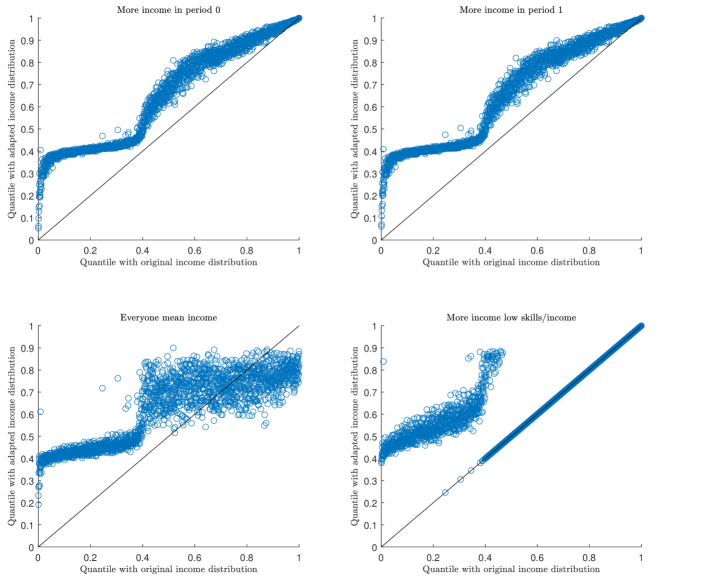
Figure 4: Skill quantiles under different investment sequences

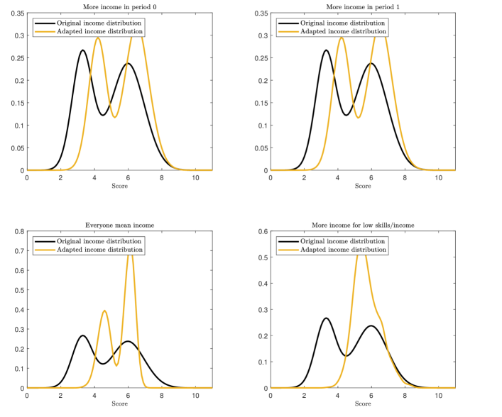
Figure 5: Outcome distributions under different investment sequences

As the last illustration, I consider how exogenous income changes affect the skill distribution. To do so, I take draws from the estimated joint distribution of income and skills in period $0$ (based on the average of the estimated parameters to get representative results) and consider four counterfactual marginal income distributions. First, I increase everyone’s income by two standard deviations in period 0. Second, I increase everyone’s income by two standard deviations in period 2. Third, I set income to the median for everyone in both periods. Fourth, I increase income by two standard deviations in both periods, but only if the initial skill and income quantiles are below $0.5$. I set all unobservables to their median values. I report results for the invariant estimator only.

I report the results in two ways. Figure 4 compares the final period skill quantiles implied by the different counterfactual income distributions with the original quantiles (one panel for each of the four cases). These results are invariant to $s_{\theta}$. Figure 5 shows the implied distribution of one of the skill measures in the final period (which could be a test score or an adult outcome in an application). These results depend on and should be interpreted relative to the units of measurements of that measures. Figure 5 is based on $s_{\theta}=1$. One can see that increasing income in either of the first two periods has very similar effects and leads to an increase in skills. Since everyone’s income increases, everyone is better off. If everyone receives the mean income, the variance of the final skill or outcome distribution decreases considerably. If we only increase income for people with low initial skills and income, then predictably, mainly the lower tail of the distribution will be affected.

4 Nonparametric identification

I now extend these results to a general nonparametric model where

(21) $$\theta_{t+1} = f_{t}(\theta_{t},I_{t},\eta_{I,t},\varsigma_{\theta,t})\hskip 91.04881ptt=0,\ldots,T-1$$

(22) $$Z_{\theta,t,m} = g_{\theta,t,m}(\theta_{t},\varepsilon_{\theta,t,m})\hskip 99.58464ptt=0,\ldots,T,\,m=1,2,3$$

(23) $$Z_{I,t,m} = g_{I,t,m}(I_{t},\varepsilon_{I,t,m})\hskip 99.58464ptt=0,\ldots,T-1,T,\,m=1,2,3$$

(24) $$I_{t} = h_{t}(\theta_{t},Y_{t},\eta_{I,t})\hskip 108.12047ptt=0,\ldots,T-1$$

(25) $$Q = r(\theta_{T},\eta_{Q})$$

Similar to CHS:10 and AW:22, in the nonparametric model, we need three measures in each period. I adapt Assumption 1 as follows.

Assumption 5.

1. $\{\{\varepsilon_{\theta,t,m}\}_{t=0,\ldots,T,m=1,2},\{\varepsilon_{I,t,m}\}_{t=0,\ldots,T-1,m=1,2},\eta_{Q}\}$ are jointly independent and independent of $\{\{\theta_{t}\}^{T}_{t=0},\{I_{t}\}^{T-1}_{t=0}\}$ conditional on $\{Y_{t}\}^{T-1}_{t=0}$.

2. All random variables are continuously distributed with strictly increasing cfds and have bounded first and second moments.

3. The joint density of $\{\{Z_{\theta,t,m}\}_{t=0,\ldots,T,m=1,2,3},\{Z_{I,t,m}\}_{t=0,\ldots,T-1,m=1,2,3},Q,\{\theta_{t}\}^{T}_{t=0},\{I_{t}\}^{T}_{t=0}\}$ is bounded conditional on $\{Y_{t}\}^{T-1}_{t=0}$ and so are all their marginal and conditional densities. $\{\{Z_{\theta,t,1}\}^{T}_{t=0},\{Z_{I,t,1}\}^{T-1}_{t=0}\}$ is bounded complete for $\{\{Z_{\theta,t,2}\}^{T}_{t=0},\{Z_{I,t,2}\}^{T-1}_{t=0}\}$ and $\{\{\theta_{t}\}^{T}_{t=0},\{I_{t}\}^{T}_{t=0}\}$ is bounded complete for $\{\{Z_{\theta,t,1}\}^{T}_{t=0},\{Z_{I,t,1}\}^{T-1}_{t=0}\}$.

4. $g_{\theta,t,m}$, $g_{I,t,m}$, and $r$ are strictly increasing in both arguments for all $m$ and $t$. $f_{t}$ and $h_{t}$ are strictly increasing the last argument for all $t$.

5. $\theta_{t}$ and $I_{t}$ have strictly positive support for all $t$.

6. $\eta_{I,t}$ is independent of $(\theta_{t},Y_{t})$ for all $t$ and $\varsigma_{\theta,t}$ is independent of $(I_{\theta},t_{t},Y_{t})$ for all $t$.

These assumptions are similar to those CHS:10, where now $\eta_{I,t}$ enters the production function directly. As a special case, suppose $f_{t}(\theta_{t},I_{t},\eta_{I,t},\varsigma_{\theta,t})=f_{t}(\theta_{t},I_{t},\kappa_{t}\eta_{I,t}+\varsigma_{\theta,t})$. Then with $\eta_{\theta,t}=\kappa_{t}\eta_{I,t}+\varsigma_{\theta,t}$, we have $E[\eta_{\theta,t}\mid\theta_{t},\eta_{I,t},Y_{t}]=\kappa_{t}\eta_{I,t}$, which is part (h) of Assumption 1. Here, the unobservables are allowed to enter much more flexibly. Parts (a) – (c) are analogous to assumptions made in CHS:10 and I build on their results to identify the joint distribution of

$$\{\{Z_{\theta,t,m}\}_{t=0,\ldots,T,m=1,2},\{Z_{I,t,m}\}_{t=0,\ldots,T-1,m=1,2},Q,\{\tilde{g}_{\theta,t}(\theta_{t})\}^{T}_{t=0},\{\tilde{g}_{I,t}(I_{t})\}^{T-1}_{t=0}\}$$

up to unknown and strictly increasing functions $\tilde{g}_{\theta,t}$ and $\tilde{g}_{I,t}$. This result is similar to the identification result in Lemma 1, which shows identification up to linear transformations. CHS:10 make an additional assumption, which ensures that the functions $\tilde{g}_{\theta,t}$ and $\tilde{g}_{I,t}$ can be pinned down (i.e. condition (v) of their Theorem 2). This assumption is similar to Assumption 2 and it is not a normalization with respect to $f_{t}$. I do not use this assumption and instead focus on features that are invariant to these monotone transformations.

Theorem 5.

Suppose Assumption 5 holds. Then

1. $F_{\theta_{t+1}}(f_{t}(Q_{\alpha_{1}}(\theta_{t}),Q_{\alpha_{2}}(I_{t}),Q_{\alpha_{3}}(\eta_{I,t}),Q_{\alpha_{4}}(\varsigma_{\theta,t})))$ is point identified for all $\alpha_{1},\alpha_{2},\alpha_{3},\alpha_{4}\in(0,1)$ such that $(Q_{\alpha_{1}}(\theta_{t}),Q_{\alpha_{3}}(I_{t}),Q_{\alpha_{2}}(\eta_{I,t}),Q_{\alpha_{4}}(\varsigma_{\theta,t}))$ is on the support of $(\theta_{t},I_{t},\eta_{I,t},\varsigma_{\theta,t})$.

2. Let

   $$I_{t}(Y)=h_{t}(Q_{\alpha_{1}}(\theta_{t}),Y,Q_{\alpha_{3}}(\eta_{I,t}))$$

   Then $F_{\theta_{t+1}}(f_{t}(Q_{\alpha_{1}}(\theta_{t}),I_{t}(Y),Q_{\alpha_{3}}(\eta_{I,t}),Q_{\alpha_{4}}(\varsigma_{\theta,t})))$ is point identified for all $\alpha_{1},\alpha_{3},\alpha_{4}\in(0,1)$.

3. $P\left(Q\leq q\mid\theta_{s}=Q_{\alpha_{1}}(\theta_{s}),\{I_{t}=Q_{\alpha_{2t}}(I_{t})\}^{T-1}_{t=0},\{\eta_{I,t}=Q_{\alpha_{3t}}(\eta_{I,t})\}^{T-1}_{t=s},\{\varsigma_{\theta,t}=Q_{\alpha_{4t}}(\varsigma_{\theta,t})\}^{T-1}_{t=s}\right)$ is point identified for all $\alpha_{1},\{\alpha_{2t},\alpha_{3t},\alpha_{4t}\}^{T-1}_{t=s}\in(0,1)$ such that the quantiles are on the joint support of the random variables.

4. $P\left(Q\leq q\mid\theta_{s}=Q_{\alpha}(\theta_{s}),\{Y_{t}=y_{t}\}^{T-1}_{t=s}\right)$ is point identified for all $\alpha\in(0,1)$.

Just as before, we can identify how investment/income and shocks affect the relative standing in the skill distribution. We can also identify the effect of a sequence of investment/income on adult outcomes, given a quantile of the initial skills. Notice that these parameters are point identified without any normalizations and they neither require scale and location restrictions on the production function nor age-invariant measures. These feature are now not only invariant to changes in the units of measurement, but to any monotone transformations of the measures. Notice that we can only identify a nonlinear transformation of the skills. Therefore, the sequence of investment that maximizes $E(\theta_{T}\mid\theta_{s}=Q_{\alpha}(\theta_{s}),\{Y_{t}=y_{t}\}^{T-1}_{t=s})$ is not point identified and choosing a particular transformation can yield erroneous conclusions regarding the role of investment. It is also important to mention that in nonadditive models, support conditions play an important role because we cannot extrapolate using the functional form. The results also implicitly contain an instrument relevancy condition because if $h_{t}$ is constant in $Y_{t}$, then $Q_{\alpha_{2}}(I_{t})$ is completely determined by $(Q_{\alpha_{1}}(\theta_{t}),Q_{\alpha_{3}}(\eta_{I,t}))$.

Another advantage of stating results without any seemingly innocuous normalizations is that one can easily impose more structure on the model without having to check and potentially adjust the normalization. For example, to reduce the dimensionality of the model, we might want to simplify the measurement system to

$$Z_{\theta,t,m} = g_{\theta,t,m}(\theta_{t}+\varepsilon_{\theta,t,m})\hskip 73.97716ptt=0,\ldots,T,m=1,2,3$$

$$Z_{I,t,m} = g_{I,t,m}(I_{t}+\varepsilon_{I,t,m})\hskip 73.97716ptt=0,\ldots,T-1,m=1,2,3$$

A normalization in the more general model might then not be a normalization in the more restrictive model. Also here, the results from Theorem 5 apply and we can identify features that are invariant to monotone transformations of the measures.

5 Conclusion

This paper is concerned with normalizations in general and skill formation models in particular. As a methodological contribution, the paper provides a formal definition of when a restriction is truly a normalization. Since restrictions typically affect many of the estimated parameters of the model, a normalization has to be with respect to some function or feature of interest, such as a subvector or a counterfactual prediction. Therefore, a restriction could be a normalization with respect to some functions, but not others. Specifically, I define a restriction as a normalization if imposing the restriction does not change the identified set of a function of interest. Normalizations are specific to a model and slight changes in the model can affect if a restriction is a normalization. When a normalization yields point identification, which is common in applications, the definition implies that all functions of interest need to be identified without normalizations. To ensure that the results are interpretable, researchers should argue that this is the case. When it is complicated to show this property formally, a standard robustness check could be to fix normalized parameters to alternative values and check how the conclusions change. It is also important that estimated parameters that depend on arbitrary normalizations might not be suitable to calibrate other models, unless one can argue that all main conclusions are unaffected by the restrictions.

In an important class of skill formation models, the paper shows that seemingly innocuous scale and location restrictions are not normalizations, can be overidentifying, and can affect parameters and counterfactuals. In particular, simply changing the units of measurements can yield ineffective investment strategies and misleading policy recommendations. The exact implications depend on the feature of interest, the production function, the measurement system, and the estimation method. To tackle these issues, the paper presents a new identification analysis, which pools all restrictions of the model and characterizes the identified set without normalizations. These results clarify which features depend on the scale and location restrictions. Importantly, many key features are invariant to these restrictions, are identified under weaker assumptions, provide robust policy implications, and are comparable across different studies.

Appendix A Additional results

A.1 Identification

Theorem 6.

Suppose Assumption 1 holds and consider the model

$$\ln\theta_{t+1} = a_{t}+\gamma_{1t}\ln\theta_{t}+\gamma_{2t}\ln I_{t}+\gamma_{3t}\ln\theta_{t}\ln I_{t}+\eta_{\theta,t}\hskip 51.21495ptt=0,\ldots,T-1$$

$$Z_{\theta,t,m} = \mu_{\theta,t,m}+\lambda_{\theta,t,m}\ln\theta_{t}+\varepsilon_{\theta,t,m}\hskip 130.88268ptt=0,\ldots,T,m=1,2$$

$$Z_{I,t,m} = \mu_{I,t,m}+\lambda_{I,t,m}\ln I_{t}+\varepsilon_{I,t,m}\hskip 130.88268ptt=0,\ldots,T-1$$

$$\ln I_{t} = \beta_{0t}+\beta_{1t}\ln\theta_{t}+\beta_{2t}\ln Y_{t}+\eta_{I,t}\hskip 116.6563ptt=0,\ldots,T-1$$

$$Q = \rho_{0}+\rho_{1}\ln\theta_{T}+\eta_{Q}$$

Then there always exist sets of observationally equivalent parameters which are consistent with the data and satisfy Assumptions 1, 2, either 3(a) or 3(b) and either 4(a) or 4(b).

Theorem 7.

Suppose Assumption 1 holds and consider the model

$$\theta_{t+1} = \left(\gamma_{1t}\theta_{t}^{\sigma_{t}}+\gamma_{2t}I_{t}^{\sigma_{t}}\right)^{\frac{\psi_{t}}{\sigma_{t}}}\exp(\eta_{\theta,t})\hskip 125.19212ptt=0,\ldots,T-1$$

$$Z_{\theta,t,m} = \mu_{\theta,t,m}+\lambda_{\theta,t,m}\ln\theta_{t}+\varepsilon_{\theta,t,m}\hskip 130.88268ptt=0,\ldots,T,m=1,2$$

$$Z_{I,t,m} = \mu_{I,t,m}+\lambda_{I,t,m}\ln I_{t}+\varepsilon_{I,t,m}\hskip 130.88268ptt=0,\ldots,T-1$$

$$\ln I_{t} = \beta_{0t}+\beta_{1t}\ln\theta_{t}+\beta_{2t}\ln Y_{t}+\eta_{I,t}\hskip 116.6563ptt=0,\ldots,T-1$$

$$Q = \rho_{0}+\rho_{1}\ln\theta_{T}+\eta_{Q}$$

where $\sigma_{t}\neq 0$ and $\gamma_{1t},\gamma_{2t}>0$ for all $t$. Then there always exist sets of observationally equivalent parameters which are consistent with the data and satisfy Assumptions 1, 2’, either 3’(a) or 3’(b) and either 4’(a) or 4’(b) and either 5’(a) or 5’(b).

Appendix B Proofs

Proof of Lemma 1.

We have

$$\begin{pmatrix}cov(Z_{\theta,s,1},Z_{\theta,t,1})\\ cov(Z_{\theta,s,1},Z_{\theta,t,2})\end{pmatrix}=\begin{pmatrix}\lambda_{\theta,s,1}\lambda_{\theta,t,1}cov(\ln\theta_{s},\ln\theta_{t})\\ \lambda_{\theta,s,1}\lambda_{\theta,t,2}cov(\ln\theta_{s},\ln\theta_{t})\end{pmatrix}$$

and

$$\begin{pmatrix}cov(Z_{I,s,1},Z_{\theta,t,1})\\ cov(Z_{I,s,1},Z_{\theta,t,2})\end{pmatrix}=\begin{pmatrix}\lambda_{I,s,1}\lambda_{\theta,t,1}cov(\ln I_{s},\ln\theta_{t})\\ \lambda_{I,s,1}\lambda_{\theta,t,2}cov(\ln I_{s},\ln\theta_{t})\end{pmatrix}$$

Since $\lambda_{\theta,t,m}\neq 0$ and $\lambda_{I,t,m}\neq 0$ for all $m$ and $t$ and $cov(\ln I_{s},\ln\theta_{t})\neq 0$ or $cov(\ln\theta_{s},\ln\theta_{t})\neq 0$ for some $s$, it follows that $\lambda_{\theta,t,1}/\lambda_{\theta,t,2}$ is identified for all $t$. Analogously, $\lambda_{I,t,1}/\lambda_{I,t,2}$ is identified for all $t$. It now follows that for $m\neq m^{\prime}$

$$\mu_{\theta,t,m}-\frac{\lambda_{\theta,t,m}}{\lambda_{\theta,t,m^{\prime}}}\mu_{\theta,t,m^{\prime}}=E\left[Z_{\theta,t,m}-\frac{\lambda_{\theta,t,m}}{\lambda_{\theta,t,m^{\prime}}}Z_{\theta,t,m^{\prime}}\right]$$

is identified as well. Now write

$$Z_{\theta,t,m} =\mu_{\theta,t,m}+\lambda_{\theta,t,m}\ln\theta_{t}+\varepsilon_{\theta,t,m}$$

$$\frac{\lambda_{\theta,t,m}}{\lambda_{\theta,t,m^{\prime}}}Z_{\theta,t,m^{\prime}}+\mu_{\theta,t,m}-\frac{\lambda_{\theta,t,m}}{\lambda_{\theta,t,m^{\prime}}}\mu_{\theta,t,m^{\prime}} =\mu_{\theta,t,m}+\lambda_{\theta,t,m}\ln\theta_{t}+\frac{\lambda_{\theta,t,m}}{\lambda_{\theta,t,m^{\prime}}}\varepsilon_{\theta,t,m^{\prime}}$$

Lemma 1 of EW:12 implies that the distributions of $\mu_{\theta,t,m}+\lambda_{\theta,t,m}\ln\theta_{t}$ and $\varepsilon_{\theta,t,m}$ are identified conditional on $Y_{1},\ldots Y_{T-1}$. Since $Q$ is another measure in period $T$, the distribution of $\eta_{Q}$ is identified as well. Similarly, the distributions of $\mu_{I,t,m}+\lambda_{I,t,m}\ln I_{t}$ and $\varepsilon_{I,t,m}$ are identified conditional on $Y_{1},\ldots Y_{T-1}$.

Next, condition on $Y_{1},\ldots Y_{T-1}$ and for any random variable $X$, let $\varphi_{X}$ be its conditional characteristic function. Then

$$\varphi_{\{Z_{\theta,t,m}\}_{t=0,\dots,T,m=1,2},\{Z_{I,t,m}\}_{t=0,\dots,T-1,m=1,2},Q}(s)$$

$$\qquad=\varphi_{\{\mu_{\theta,t,m}+\lambda_{\theta,t,m}\ln\theta_{t}\}_{t=0,\dots,T,m=1,2},\{\mu_{I,t,m}+\lambda_{I,t,m}\ln I_{t}\}_{t=0,\dots,T-1,m=1,2},\rho_{0}+\rho_{1}\ln\theta_{T}}(s)$$

$$\qquad\qquad\times\varphi_{\{\varepsilon_{\theta,t,m}\}_{t=0,\dots,T,m=1,2},\{\varepsilon_{I,t,m}\}_{t=0,\dots,T-1,m=1,2},\eta}(s)$$

Since the measurement errors are independent and the marginal distributions are identified, the joint distribution is identified. That is, $\varphi_{\{\varepsilon_{\theta,t,m}\}_{t=0,\dots,T,m=1,2},\{\varepsilon_{I,t,m}\}_{t=0,\dots,T-1,m=1,2},\eta}(s)$ is identified. It follows that $\varphi_{\{\mu_{\theta,t,m}+\lambda_{\theta,t,m}\ln\theta_{t}\}_{t=0,\dots,T,m=1,2},\{\mu_{I,t,m}+\lambda_{I,t,m}\ln I_{t}\}_{t=0,\dots,T-1,m=1,2},\rho_{0}+\rho_{1}\ln\theta_{T}}(s)$ is identified for all nonzeros of $\varphi_{\{\varepsilon_{\theta,t,m}\}_{t=0,\dots,T,m=1,2},\{\varepsilon_{I,t,m}\}_{t=0,\dots,T-1,m=1,2},\eta}(s)$. Since the zeros of this function are isolated and since characteristics functions are continuous, the characteristic function of $\{\mu_{\theta,t,m}+\lambda_{\theta,t,m}\ln\theta_{t}\}_{t=0,\dots,T,m=1,2},\{\mu_{I,t,m}+\lambda_{I,t,m}\ln I_{t}\}_{t=0,\dots,T-1,m=1,2},\rho_{0}+\rho_{1}\ln\theta_{T}$ and therefore its joint distribution is identified.

∎

Proof of Theorem 1.

I first show that $\{\tilde{\mu}_{\theta,t,m},\tilde{\lambda}_{\theta,t,m}\}_{t=0,\ldots,T,m=1,2}$, $\{\tilde{\mu}_{I,t,m},\tilde{\lambda}_{I,t,m}\}_{t=0,\ldots,T-1,m=1,2}$, $\{\tilde{a}_{t},\tilde{\gamma}_{1t},\tilde{\gamma}_{2t},\tilde{\gamma}_{3t}\}^{T-1}_{t=0}$, $\{\tilde{\beta}_{0t},\tilde{\beta}_{1t},\tilde{\beta}_{2t}\}^{T-1}_{t=0}$, and $(\tilde{\rho}_{0},\tilde{\rho}_{1})$ are identified. By Lemma 1 the joint distribution of $(\{\ln\tilde{\theta}_{t}\}_{t=0,\dots,T,m=1,2},\{\ln\tilde{I}_{t}\}_{t=0,\dots,T-1,m=1,2},Q)$ is point identified conditional on $(Y_{0},\ldots,Y_{T-1})$. The proof of that lemma also implies that we can identify the distributions of ${\varepsilon}_{\theta,t,m}$ and ${\varepsilon}_{I,t,m}$ and thus, also $\tilde{\mu}_{\theta,t,m}$, $\tilde{\lambda}_{\theta,t,m}$, $\tilde{\mu}_{I,t,m}$, and $\tilde{\lambda}_{I,t,m}$ for all $m$ and $t$. From the identified joint distribution, we also know

$$E[\ln\tilde{I}_{t}\mid\tilde{\theta}_{t},Y_{t}]=\tilde{\beta}_{0t}+\tilde{\beta}_{1t}\ln\tilde{\theta}_{t}+\tilde{\beta}_{2t}\ln Y_{t}$$

and thus, we can identify $\tilde{\beta}_{0t}$, $\tilde{\beta}_{1t}$, and $\tilde{\beta}_{2t}$. Similarly, $E[\ln\tilde{I}_{t}\mid Q]$ and therefore $\tilde{\rho}_{0}$ and $\tilde{\rho}_{1}$ are identified.

We can also identify $E[\ln\tilde{\theta}_{t+1}\mid\tilde{\theta}_{t},\tilde{I}_{t},Y_{t}]$ we can write as

$$E[\ln\tilde{\theta}_{t+1}\mid\tilde{\theta}_{t},\tilde{I}_{t},Y_{t}] =\tilde{a}_{t}+\tilde{\gamma}_{1t}\ln\tilde{\theta}_{t}+\tilde{\gamma}_{2t}\ln\tilde{I}_{t}+\tilde{\gamma}_{3t}\ln\tilde{\theta}_{t}\ln\tilde{I}_{t}+E[\tilde{\eta}_{\theta,t}\mid\tilde{\theta}_{t},\tilde{I}_{t},Y_{t}]$$

$$=\tilde{a}_{t}+\tilde{\gamma}_{1t}\ln\tilde{\theta}_{t}+\tilde{\gamma}_{2t}\ln\tilde{I}_{t}+\tilde{\gamma}_{3t}\ln\tilde{\theta}_{t}\ln\tilde{I}_{t}+\lambda_{\theta,t+1,1}E[\eta_{\theta,t}\mid\tilde{\theta}_{t},\tilde{\eta}_{I,t},Y_{t}]$$

$$=\tilde{a}_{t}+\tilde{\gamma}_{1t}\ln\tilde{\theta}_{t}+\tilde{\gamma}_{2t}\ln\tilde{I}_{t}+\tilde{\gamma}_{3t}\ln\tilde{\theta}_{t}\ln\tilde{I}_{t}+\lambda_{\theta,t+1,1}E[\eta_{\theta,t}\mid\tilde{\eta}_{I,t}]$$

$$=\tilde{a}_{t}+\tilde{\gamma}_{1t}\ln\tilde{\theta}_{t}+\tilde{\gamma}_{2t}\ln\tilde{I}_{t}+\tilde{\gamma}_{3t}\ln\tilde{\theta}_{t}\ln\tilde{I}_{t}+(\lambda_{\theta,t+1,1}/\lambda_{I,t,1})\kappa_{t}\tilde{\eta}_{I,t}$$

The second line follows because $\tilde{\theta}_{t},\tilde{I}_{t},Y_{t}$ is identical to conditioning on $\tilde{\theta}_{t},\tilde{\eta}_{I,t},Y_{t}$ due to the line relationship in equation (9). The third and fourth line follow from Assumption 1(b) and the relationship $\tilde{\eta}_{I,t}=\lambda_{I,t,1}{\eta}_{I,t}$. Hence, we can identify $\tilde{a}_{t}$, $\tilde{\gamma}_{1t}$, $\tilde{\gamma}_{2t}$, $\tilde{\gamma}_{3t}$, and $(\lambda_{\theta,t+1,1}/\lambda_{I,t,1})\kappa_{t}$ by regressing $\ln\tilde{\theta}_{t+1}$ on $\ln\tilde{\theta}_{t}$, $\ln\tilde{I}_{t}$, $\ln\tilde{I}_{t}$, and $\tilde{\eta}_{I,t}=\ln\tilde{I}_{t}-\tilde{\beta}_{0t}-\tilde{\beta}_{1t}\ln\tilde{\theta}_{t}-\tilde{\beta}_{2t}\ln Y_{t}$.

Now suppose we have an alternative set of parameters, denoted by $\{\bar{\mu}_{\theta,t,m},\bar{\lambda}_{\theta,t,m}\}_{t=0,\ldots,T,m=1,2}$, $\{\bar{\mu}_{I,t,m},\bar{\lambda}_{I,t,m}\}_{t=0,\ldots,T-1,m=1,2}$, $\{\bar{a}_{t},\bar{\gamma}_{1t},\bar{\gamma}_{2t},\bar{\gamma}_{3t}\}^{T-1}_{t=0}$, $\{\bar{\beta}_{0t},\bar{\beta}_{1t},\bar{\beta}_{2t}\}^{T-1}_{t=0}$, and $(\bar{\rho}_{0},\bar{\rho}_{1})$ that yields the same values of $\{\tilde{\mu}_{\theta,t,m},\tilde{\lambda}_{\theta,t,m}\}_{t=0,\ldots,T,m=1,2}$, $\{\tilde{\mu}_{I,t,m},\tilde{\lambda}_{I,t,m}\}_{t=0,\ldots,T-1,m=1,2}$, $\{\tilde{\beta}_{0t},\tilde{\beta}_{1t},\tilde{\beta}_{2t}\}^{T-1}_{t=0}$, $(\tilde{\rho}_{0},\tilde{\rho}_{1})$, and $\{\tilde{a}_{t},\tilde{\gamma}_{1t},\tilde{\gamma}_{2t},\tilde{\gamma}_{3t}\}^{T-1}_{t=0}$. Define $\bar{\theta}_{t}$ and $\bar{I}_{t}$ such that

$$\bar{\mu}_{\theta,t,1}+\bar{\lambda}_{\theta,t,1}\ln\bar{\theta}_{t}={\mu}_{\theta,t,1}+{\lambda}_{\theta,t,1}\ln{\theta}_{t}=\ln\tilde{\theta}_{t}$$

and

$$\bar{\mu}_{I,t,1}+\bar{\lambda}_{I,t,1}\ln\bar{I}_{t}={\mu}_{I,t,1}+{\lambda}_{I,t,1}\ln{I}_{t}=\ln\tilde{I}_{t}$$

For $m\neq 1$, we then have

$$\bar{\mu}_{\theta,t,m}+\bar{\lambda}_{\theta,t,m}\ln\bar{\theta}_{t} =\bar{\mu}_{\theta,t,m}+\bar{\lambda}_{\theta,t,m}\left(\ln\tilde{\theta}_{t}-\bar{\mu}_{\theta,t,1}\right)/\bar{\lambda}_{\theta,t,1}$$

$$=\bar{\mu}_{\theta,t,m}-\frac{\bar{\lambda}_{\theta,t,m}}{\bar{\lambda}_{\theta,t,1}}+\frac{\bar{\lambda}_{\theta,t,m}}{\bar{\lambda}_{\theta,t,1}}\ln\tilde{\theta}_{t}$$

$$=\tilde{\mu}_{\theta,t,m}+\tilde{\lambda}_{\theta,t,m}\ln\tilde{\theta}_{t}$$

and similarly

$$\bar{\mu}_{I,t,m}+\bar{\lambda}_{I,t,m}\ln\bar{I}_{t} =\tilde{\mu}_{I,t,m}+\tilde{\lambda}_{I,t,m}\ln\tilde{I}_{t}.$$

Then the two models generate the same distribution of the measures. In addition, the parameters and $\bar{\theta}_{t}$ are consistent with the production technology because

$$\bar{\mu}_{\theta,t+1,1} +\bar{\lambda}_{\theta,t+1,1}\ln\bar{\theta}_{t+1}$$

$$=\ln\tilde{\theta}_{t+1}$$

$$=\tilde{a}_{t}+\tilde{\gamma}_{1t}\ln\tilde{\theta}_{t}+\tilde{\gamma}_{2t}\ln I_{t}+\tilde{\gamma}_{3t}\ln\tilde{\theta}_{t}\ln I_{t}+\tilde{\eta}_{\theta,t}$$

$$=\tilde{a}_{t}+\tilde{\gamma}_{1t}(\bar{\mu}_{\theta,t,1}+\bar{\lambda}_{\theta,t,1}\ln\bar{\theta}_{t})+\tilde{\gamma}_{2t}\ln I_{t}+\tilde{\gamma}_{3t}\ln(\bar{\mu}_{\theta,t,1}+\bar{\lambda}_{\theta,t,1}\ln\bar{\theta}_{t})\ln I_{t}+\tilde{\eta}_{\theta,t}$$

$$=\tilde{a}_{t}+\tilde{\gamma}_{1t}(\bar{\mu}_{\theta,t,1}+\bar{\lambda}_{\theta,t,1}\ln\bar{\theta}_{t})+\tilde{\gamma}_{2t}\ln I_{t}+\tilde{\gamma}_{3t}\ln(\bar{\mu}_{\theta,t,1}+\bar{\lambda}_{\theta,t,1}\ln\bar{\theta}_{t})\ln I_{t}+\tilde{\eta}_{\theta,t}$$

Since

$$\tilde{a}_{t}=\bar{\lambda}_{\theta,t+1,1}\bar{a}_{t}+\bar{\mu}_{\theta,t+1,1}-\frac{\bar{\lambda}_{\theta,t+1,1}}{\bar{\lambda}_{\theta,t,1}}\bar{\mu}_{\theta,t,1}\bar{\gamma}_{1t}-\frac{\bar{\lambda}_{\theta,t+1,1}}{\bar{\lambda}_{I,t,1}}\mu_{I,t,1}\bar{\gamma}_{2t}$$

$$\tilde{\gamma}_{1t}=\bar{\lambda}_{\theta,t+1,1}\left(\frac{1}{\bar{\lambda}_{\theta,t,1}}\bar{\gamma}_{1t}-\frac{\bar{\mu}_{I,t,1}}{\bar{\lambda}_{I,t,1}}\bar{\gamma}_{3t}\right),\;\;\tilde{\gamma}_{2t}=\bar{\lambda}_{\theta,t+1,1}\left(\frac{\bar{\gamma}_{2t}}{\bar{\lambda}_{I,t,1}}-\frac{\bar{\mu}_{\theta,t,1}}{\bar{\lambda}_{\theta,t,1}}\bar{\gamma}_{3t}\right),\;\;\tilde{\gamma}_{3t}=\frac{\bar{\lambda}_{\theta,t+1,1}}{\bar{\lambda}_{\theta,t,1}\bar{\lambda}_{I,t,1}}\bar{\gamma}_{3t}$$

and $\tilde{\eta}_{\theta,t}=\lambda_{\theta,t+1,1}{\eta}_{\theta,t}$, it is easy to show that

$$\ln\bar{\theta}_{t+1} =\bar{a}_{t}+\bar{\gamma}_{1t}\ln\bar{\theta}_{t}+\bar{\gamma}_{2t}\ln I_{t}+\bar{\gamma}_{3t}\ln\bar{\theta}_{t}\ln I_{t}+\bar{\eta}_{\theta,t}$$

with $\bar{\eta}_{\theta,t}=\frac{\lambda_{\theta,t+1,1}}{\bar{\lambda}_{\theta,t+1,1}}{\eta}_{\theta,t}$.

Analogously, one can show that

$$\ln\bar{I}_{t} =\bar{\beta}_{0t}+\bar{\beta}_{1t}\ln\theta_{t}+\bar{\beta}_{2t}\ln Y_{t}+\bar{\eta}_{I,t}$$

$$Q =\bar{\rho}_{0}+\bar{\rho}_{1}\ln\bar{\theta}_{T}+\bar{\eta}_{Q}$$

For the last part first notice that once $\{\lambda_{\theta,t,1},\lambda_{I,t,1},\mu_{\theta,t,1},\mu_{I,t,1}\}_{t=1,\ldots,T}$ are fixed, the vector $\{\lambda_{\theta,t,m},\lambda_{I,t,m},\mu_{\theta,t,m},\mu_{I,t,m}\}_{t=1,\ldots,T}$ is uniquely determined for all $m\neq 1$ due to the restrictions the parameters in the identified set have to satisfy. From these restrictions, we can then uniquely determine $\gamma_{3t}$ and with that parameter also $\gamma_{1t}$ and $\gamma_{2t}$. Similarly, all the other parameters are uniquely determined. We then found the unique parameter vector for which $\{\lambda_{\theta,t,1},\lambda_{I,t,1},\mu_{\theta,t,1},\mu_{I,t,1}\}_{t=1,\ldots,T}$ are fixed and that yields the same values of $\{\tilde{\mu}_{\theta,t,m},\tilde{\lambda}_{\theta,t,m}\}_{t=0,\ldots,T,m=1,2}$, $\{\tilde{\mu}_{I,t,m},\tilde{\lambda}_{I,t,m}\}_{t=0,\ldots,T-1,m=1,2}$, $\{\tilde{a}_{t},\tilde{\gamma}_{1t},\tilde{\gamma}_{2t},\tilde{\gamma}_{3t}\}^{T-1}_{t=0}$, $(\tilde{\rho}_{0},\tilde{\rho}_{1})$, and $\{\tilde{\beta}_{0t},\tilde{\beta}_{1t},\tilde{\beta}_{2t}\}^{T-1}_{t=0}$.

∎

Proof of Corollary 1.

The last part of Theorem 1 immediately implies that all parameters are point identified under Assumptions 1, 2, 3(a), and 4(a). Now suppose Assumptions 1, 2, 3(b), and 4(a) hold. Then, since $a_{t}=\mu_{I,t,1}=0$, $\mu_{\theta,t+1,1}-\mu_{\theta,t,1}\frac{\lambda_{\theta,t+1,1}}{\lambda_{\theta,t,1}}\gamma_{1t}$ is identified. In addition $\frac{\lambda_{\theta,t+1,1}}{\lambda_{\theta,t,1}}\gamma_{1t}$ is identified. We also know that $\mu_{\theta,0,1}=0$, which identifies $\mu_{\theta,1,1}$ and then we can recursively identify $\mu_{\theta,t,1}$ for all $t$. In addition, we can identify $\lambda_{\theta,t+1,1}\gamma_{2t}$ because $\lambda_{\theta,t+1,1}\left(\gamma_{2t}-\frac{\mu_{\theta,t,1}}{\lambda_{\theta,t,1}}\gamma_{3t}\right)$, $\frac{\lambda_{\theta,t+1,1}}{\lambda_{\theta,t,1}}\gamma_{3t}$, and $\mu_{\theta,t,1}$ are identified. Next notice that, we can also identify

$$\frac{\lambda_{\theta,t+1,1}}{\lambda_{\theta,t,1}}\gamma_{1t}=\frac{\lambda_{\theta,t+1,1}}{\lambda_{\theta,t,1}}(1-\gamma_{2t}-\gamma_{3t})=\frac{\lambda_{\theta,t+1,1}}{\lambda_{\theta,t,1}}-\frac{\lambda_{\theta,t+1,1}}{\lambda_{\theta,t,1}}\gamma_{2t}-\frac{\lambda_{\theta,t+1,1}}{\lambda_{\theta,t,1}}\gamma_{3t}$$

Since $\lambda_{\theta,0,1}=1$, we can identify $\lambda_{\theta,1,1}$ and then, using the previous equation, $\lambda_{\theta,t,1}$ recursively for all $t$. Once we know $\mu_{\theta,t,1}$ and $\lambda_{\theta,t,1}$ for all $t$, identification of the production function parameters follows immediately. In addition, since $\frac{\lambda_{\theta,t,m}}{\lambda_{\theta,t,1}}$ and $\mu_{\theta,t,m}+\left(\lambda_{\theta,t,m}/\lambda_{\theta,t,1}\right)\mu_{\theta,t,1}$ are identified, we can identify $\lambda_{\theta,t,m}$ and $\mu_{\theta,t,m}$ for all $m$. It then also immediately follows that $\beta_{0t}$, $\beta_{1t}$, $\beta_{2t}$, $\rho_{0}$, and $\rho_{1}$ are identified.

Now suppose Assumptions 1, 2, 3(a), and 4(b) hold. Then, using the argument as in the proof of Theorem 1, $\{\lambda_{\theta,t,m},\mu_{\theta,t,m},\}_{t=1,\ldots,T}$ is uniquely determined. Next, using the expressions for $\tilde{\beta}_{1t}$ and $\tilde{\beta}_{2t}$ and $\beta_{1t}+\beta_{2t}=1$, we can identify $\beta_{1t}$, $\beta_{2t}$, and $\lambda_{I,t,1}$. With $\tilde{\beta}_{0t}$ and $\beta_{0t}=0$, we can uniquely determine $\mu_{I,t,1}$. Once the coefficients in the measurement error equation are identified for one of the measures, the second part of Theorem 1 implies that all other parameters are identified as well.

Finally suppose Assumptions 1, 2, 3(b), and 4(b) hold. Then, using $\beta_{0t}=0$ and $\beta_{1t}+\beta_{2t}=1$ we can write $\tilde{\beta}_{0t}=\mu_{I,t,1}-\tilde{\beta}_{1t}\mu_{\theta,t,1}$ and $\lambda_{\theta,t,1}\tilde{\beta}_{1t}+\tilde{\beta}_{2t}=\lambda_{I,t,1}$. Now assume that $\mu_{\theta,t,1}$ and $\lambda_{\theta,t,1}$, are identified. Then $\mu_{I,t,1}$ and $\lambda_{I,t,1}$ are also identified. Notice that since $\gamma_{1t}+\gamma_{2t}+\gamma_{2t}=1$, we have

$$\frac{\tilde{\gamma}_{1t}}{\lambda_{I,t,1}}+\frac{\tilde{\gamma}_{2t}}{\lambda_{\theta,t,1}}+\tilde{\gamma}_{3t}=\frac{\lambda_{\theta,t+1,1}}{{\lambda_{\theta,t,1}\lambda_{I,t,1}}}-\mu_{I,t,1}\frac{\lambda_{\theta,t,1}}{\lambda_{I,t,1}}\tilde{\gamma}_{3t}-\mu_{\theta,t,1}\frac{\lambda_{I,t,1}}{\lambda_{\theta,t,1}}\tilde{\gamma}_{3t}$$

and thus, $\lambda_{\theta,t+1,1}$ and $\lambda_{I,t+1,1}=\lambda_{\theta,t+1,1}\tilde{\beta}_{1,t+1}+\tilde{\beta}_{2,t+1}$ are identified. Then $\gamma_{1t}$, $\gamma_{2t}$, and $\gamma_{3t}$ are also identified. Using the expression for $\tilde{a}_{t}$ together with $a_{t}=0$ then identifies $\mu_{\theta,t+1,1}$ and $\mu_{I,t+1,1}=\tilde{\beta}_{0,t+1}+\tilde{\beta}_{1,t+1}\mu_{\theta,t+1,1}$. Since $\mu_{\theta,0,1}=0$ and $\lambda_{\theta,0,1}=1$, these arguments imply that $\mu_{\theta,t,1}$, $\mu_{I,t,1}$, $\lambda_{\theta,t,1}$, and $\lambda_{I,t,1}$, are identified for all $t$. Once the coefficients in the measurement error equation are identified for one of the measures, the second part of Theorem 1 implies that all other parameters are identified as well.

∎

Proof of Theorem 2.

For the first part, notice that

$$F_{\ln\tilde{\theta}_{t+1}}(\tilde{a}_{t}+\tilde{\gamma}_{1t}\ln Q_{\alpha_{1}}(\tilde{\theta}_{t})+\tilde{\gamma}_{2t}\ln Q_{\alpha_{2}}(\tilde{I}_{t})+\tilde{\gamma}_{3t}\ln Q_{\alpha_{1}}(\tilde{\theta}_{t})\ln Q_{\alpha_{2}}(\tilde{I}_{t})+Q_{\alpha_{3}}(\tilde{\eta}_{\theta,t}))$$

$$= F_{\ln\tilde{\theta}_{t+1}}\left(\tilde{a}_{t}+\tilde{\gamma}_{1t}Q_{\alpha_{1}}(\mu_{\theta,t,1}+\lambda_{\theta,t,1}\ln\theta_{t})+\tilde{\gamma}_{2t}Q_{\alpha_{2}}(\mu_{I,t,1}+\lambda_{I,t,1}\ln I_{t})\right.$$

$$\qquad\qquad+\left.\tilde{\gamma}_{3t}Q_{\alpha_{1}}(\mu_{\theta,t,1}+\lambda_{\theta,t,1}\ln\theta_{t})Q_{\alpha_{2}}(\mu_{I,t,1}+\lambda_{I,t,1}\ln I_{t})+Q_{\alpha_{3}}(\lambda_{\theta,t+1,1}\eta_{\theta,t})\right)$$

$$= F_{\ln\tilde{\theta}_{t+1}}\left(\tilde{a}_{t}+\tilde{\gamma}_{1t}(\mu_{\theta,t,1}+\lambda_{\theta,t,1}Q_{\alpha_{1}}\ln(\theta_{t}))+\tilde{\gamma}_{2t}(\mu_{I,t,1}+\lambda_{I,t,1}Q_{\alpha_{2}}(\ln I_{t}))\right.$$

$$\qquad\qquad+\left.\tilde{\gamma}_{3t}(\mu_{\theta,t,1}+\lambda_{\theta,t,1}Q_{\alpha_{1}}\ln(\theta_{t}))(\mu_{I,t,1}+\lambda_{I,t,1}Q_{\alpha_{2}}(\ln I_{t}))+\lambda_{\theta,t+1,1}Q_{\alpha_{3}}(\eta_{\theta,t})\right)$$

$$= F_{\ln\tilde{\theta}_{t+1}}\left(\mu_{t+1}+\lambda_{t+1}\left({a}_{t}+{\gamma}_{1t}Q_{\alpha_{1}}\ln(\theta_{t})+{\gamma}_{2t}Q_{\alpha_{2}}(\ln I_{t})+{\gamma}_{3t}Q_{\alpha_{1}}\ln(\theta_{t})Q_{\alpha_{2}}(\ln I_{t})+Q_{\alpha_{3}}(\eta_{\theta,t})\right)\right)$$

$$= F_{\ln{\theta}_{t+1}}\left({a}_{t}+{\gamma}_{1t}Q_{\alpha_{1}}\ln(\theta_{t})+{\gamma}_{2t}Q_{\alpha_{2}}(\ln I_{t})+{\gamma}_{3t}Q_{\alpha_{1}}\ln(\theta_{t})Q_{\alpha_{2}}(\ln I_{t})+Q_{\alpha_{3}}(\eta_{\theta,t})\right)$$

Since the joint distribution of $\left(\{\ln\tilde{\theta}_{t}\}_{t=0,\dots,T},\{\ln\tilde{I}_{t}\}_{t=0,\dots,T-1}\right)$ and $\tilde{a}_{t}$, $\tilde{\gamma}_{1t}$, $\tilde{\gamma}_{2t}$, and $\tilde{\gamma}_{3t}$ are identified and since $\tilde{\eta}_{\theta,t}=\ln\tilde{\theta}_{t+1}-\left(\tilde{a}_{t}+\tilde{\gamma}_{1t}\ln\tilde{\theta}_{t}+\tilde{\gamma}_{2t}\ln I_{t}+\tilde{\gamma}_{3t}\ln\tilde{\theta}_{t}\ln I_{t}\right)$, it follows that

$$F_{\ln\tilde{\theta}_{t+1}}(\tilde{a}_{t}+\tilde{\gamma}_{1t}\ln Q_{\alpha_{1}}(\tilde{\theta}_{t})+\tilde{\gamma}_{2t}\ln Q_{\alpha_{2}}(\tilde{I}_{t})+\tilde{\gamma}_{3t}\ln Q_{\alpha_{1}}(\tilde{\theta}_{t})\ln Q_{\alpha_{2}}(\tilde{I}_{t})+Q_{\alpha_{3}}(\tilde{\eta}_{\theta,t}))$$

and therefore

$$F_{\ln{\theta}_{t+1}}\left({a}_{t}+{\gamma}_{1t}Q_{\alpha_{1}}\ln(\theta_{t})+{\gamma}_{2t}Q_{\alpha_{2}}(\ln I_{t})+{\gamma}_{3t}Q_{\alpha_{1}}\ln(\theta_{t})Q_{\alpha_{2}}(\ln I_{t})+Q_{\alpha_{3}}(\eta_{\theta,t})\right)$$

is point identified.

For the second part notice that

$$\ln\tilde{I}_{t}(Y) =\tilde{\beta}_{0t}+\tilde{\beta}_{1t}\ln Q_{\alpha_{1}}(\tilde{\theta}_{t})+\tilde{\beta}_{2t}\ln Y+Q_{\alpha_{4}}(\tilde{\eta}_{I,t})$$

$$=\tilde{\beta}_{0t}+\tilde{\beta}_{1t}(\mu_{\theta,t,1}+\lambda_{\theta,t,1}Q_{\alpha_{1}}\ln(\theta_{t}))+\tilde{\beta}_{2t}\ln Y+Q_{\alpha_{4}}(\lambda_{I,t,1}{\eta}_{I,t})$$

$$=\mu_{I,t,1}+\lambda_{I,t,1}\left(\beta_{0t}+\beta_{1t}Q_{\alpha_{1}}(\ln(\theta_{t}))+{\beta}_{2t}\ln Y+Q_{\alpha_{4}}({\eta}_{I,t})\right)$$

$$=\mu_{I,t,1}+\lambda_{I,t,1}\ln I_{t}(Y)$$

is identified. Then using the same arguments as above, it follows

$$F_{\ln\tilde{\theta}_{t+1}}(\tilde{a}_{t}+\tilde{\gamma}_{1t}\ln Q_{\alpha_{1}}(\tilde{\theta}_{t})+\tilde{\gamma}_{2t}\ln\tilde{I}_{t}(Y)+\tilde{\gamma}_{3t}\ln Q_{\alpha_{1}}(\tilde{\theta}_{t})\ln\tilde{I}_{t}(Y)+Q_{\alpha_{3}}(\tilde{\eta}_{\theta,t}))$$

$$=F_{\ln\theta_{t+1}}(a_{t}+\gamma_{1t}\ln Q_{\alpha_{1}}(\theta_{t})+\gamma_{2t}\ln I_{t}(Y)+\gamma_{3t}\ln Q_{\alpha_{1}}(\theta_{t})\ln I_{t}(Y)+Q_{\alpha_{3}}(\eta_{\theta,t}))$$

is point identified for all $\alpha_{1},\alpha_{3},\alpha_{4}\in(0,1)$.

For the third part we have

$$P\left(Q\leq q\mid\theta_{t}=Q_{\alpha_{1}}(\theta_{t}),\{I_{s}=Q_{\alpha_{2s}}(I_{s})\}^{T-1}_{s=t},\{\eta_{\theta,s}=Q_{\alpha_{3s}}(\eta_{\theta,s})\}^{T-1}_{s=t}\right)$$

$$=P\left(Q\leq q\mid\tilde{\theta}_{t}=Q_{\alpha_{1}}(\tilde{\theta}_{t}),\{\tilde{I}_{s}=Q_{\alpha_{2s}}(\tilde{I}_{s})\}^{T-1}_{s=t},\{\tilde{\eta}_{\theta,s}=Q_{\alpha_{3s}}(\tilde{\eta}_{\theta,s})\}^{T-1}_{s=t}\right)$$

and hence, the left hand is identified.

The fourth part follows from identification of the joint distribution of $(Q,\tilde{\theta}_{t},\{Y_{s}\}^{T-1}_{s=t})$

Finally, notice that

$$\tilde{\gamma}_{1t}+\tilde{\gamma}_{3t}\ln\tilde{I}_{t}=\frac{\lambda_{\theta,t+1,1}}{\lambda_{\theta,t,1}}\left(\gamma_{1t}+\gamma_{3t}\ln I_{t}\right)$$

whose distribution is identified under Assumption 3(a).

∎

Proof of Theorem 3 .

The same arguments as in the proof of Theorem 1 implies that $\tilde{\beta}_{0t}$, $\tilde{\beta}_{1t}$, $\tilde{\beta}_{2t}$, $\tilde{\rho}_{0}$ and $\tilde{\rho}_{1}$ are identified. Moreover, we can also identify $E[\ln\tilde{\theta}_{t+1}\mid\tilde{\theta}_{t},\tilde{I}_{t},Y_{t}]$ which we can write as

$$E[\ln\tilde{\theta}_{t+1}\mid\tilde{\theta}_{t},\tilde{I}_{t},Y_{t}] =\frac{\lambda_{\theta,t+1,1}\psi_{t}}{{\sigma}_{t}}\ln\left(\tilde{\gamma}_{1t}\tilde{\theta}_{t}^{\frac{{\sigma}_{t}}{\lambda_{\theta,t,1}}}+\tilde{\gamma}_{2t}\tilde{I}_{t}^{\frac{{\sigma}_{t}}{\lambda_{I,t,1}}}\right)+E[\tilde{\eta}_{\theta,t}\mid\tilde{\theta}_{t},\tilde{I}_{t},Y_{t}]$$

$$=\frac{\lambda_{\theta,t+1,1}\psi_{t}}{{\sigma}_{t}}\ln\left(\tilde{\gamma}_{1t}\tilde{\theta}_{t}^{\frac{{\sigma}_{t}}{\lambda_{\theta,t,1}}}+\tilde{\gamma}_{2t}\tilde{I}_{t}^{\frac{{\sigma}_{t}}{\lambda_{I,t,1}}}\right)+(\lambda_{\theta,t+1,1}/\lambda_{I,t,1})\kappa_{t}\tilde{\eta}_{I,t}$$

Hence

$$\frac{\frac{\partial E[\ln\tilde{\theta}_{t+1}\mid\tilde{\theta}_{t},\tilde{I}_{t},Y_{t}]}{\partial\tilde{\theta}_{t}}}{\frac{\partial E[\ln\tilde{\theta}_{t+1}\mid\tilde{\theta}_{t},\tilde{I}_{t},Y_{t}]}{\partial\tilde{I}_{t}}} =\frac{\lambda_{I,t,1}}{\lambda_{\theta,t,1}}\frac{\tilde{\gamma}_{1t}}{\tilde{\gamma}_{2t}}\tilde{\theta}_{t}^{\frac{{\sigma}_{t}}{\lambda_{\theta,t,1}}-1}\tilde{I}_{t}^{1-\frac{{\sigma}_{t}}{\lambda_{I,t,1}}}$$

which identifies $\frac{\lambda_{I,t,1}}{\lambda_{\theta,t,1}}\frac{\tilde{\gamma}_{1t}}{\tilde{\gamma}_{2t}}$, $\frac{{\sigma}_{t}}{\lambda_{\theta,t,1}}$ and $\frac{{\sigma}_{t}}{\lambda_{I,t,1}}$. Hence, $\frac{\tilde{\gamma}_{1t}}{\tilde{\gamma}_{2t}}$ is identified. In addition $(\lambda_{\theta,t+1,1}/\lambda_{I,t,1})\kappa_{t}$ is identified. Now write

$$E[\ln\tilde{\theta}_{t+1}\mid\tilde{\theta}_{t},\tilde{I}_{t},Y_{t}] =\frac{\lambda_{\theta,t+1,1}\psi_{t}}{{\sigma}_{t}}\ln\left(\frac{\tilde{\gamma}_{1t}}{\tilde{\gamma}_{2t}}\tilde{\theta}_{t}^{\frac{{\sigma}_{t}}{\lambda_{\theta,t,1}}\psi_{t}}+\tilde{I}_{t}^{\frac{{\sigma}_{t}}{\lambda_{I,t,1}}}\right)+\frac{\lambda_{\theta,t+1,1}\psi_{t}}{{\sigma}_{t}}\ln\tilde{\gamma}_{2t}+(\lambda_{\theta,t+1,1}/\lambda_{I,t,1})\kappa_{t}\tilde{\eta}_{I,t}$$

which is linear in $\ln\left(\frac{\tilde{\gamma}_{1t}}{\tilde{\gamma}_{2t}}\tilde{\theta}_{t}^{\frac{{\sigma}_{t}}{\lambda_{\theta,t,1}}}+\tilde{I}_{t}^{\frac{{\sigma}_{t}}{\lambda_{I,t,1}}}\right)$ and therefore $\frac{\lambda_{\theta,t+1,1}\psi_{t}}{{\sigma}_{t}}$ and $\frac{\lambda_{\theta,t+1,1}\psi_{t}}{{\sigma}_{t}}\ln\tilde{\gamma}_{2t}$ are identified. Hence $\tilde{\gamma}_{1t}$ and $\tilde{\gamma}_{2t}$ are identified.

Now suppose we have an alternative set of parameters, denoted by $\{\bar{\mu}_{\theta,t,m},\bar{\lambda}_{\theta,t,m}\}_{t=0,\ldots,T,m=1,2}$, $\{\bar{\mu}_{I,t,m},\bar{\lambda}_{I,t,m}\}_{t=0,\ldots,T-1,m=1,2}$, $\{\bar{a}_{t},\bar{\gamma}_{1t},\bar{\gamma}_{2t},\bar{\gamma}_{3t},\bar{\psi}_{t}\}^{T-1}_{t=0}$, $\{\bar{\beta}_{0t},\bar{\beta}_{1t},\bar{\beta}_{2t}\}^{T-1}_{t=0}$, and $(\bar{\rho}_{0},\bar{\rho}_{1})$ that yields the same values of $\{\tilde{\mu}_{\theta,t,m},\tilde{\lambda}_{\theta,t,m}\}_{t=0,\ldots,T,m=1,2}$, $\{\tilde{\mu}_{I,t,m},\tilde{\lambda}_{I,t,m}\}_{t=0,\ldots,T-1,m=1,2}$, $\{\tilde{\beta}_{0t},\tilde{\beta}_{1t},\tilde{\beta}_{2t}\}^{T-1}_{t=0}$, $\{\tilde{\gamma}_{1t},\tilde{\gamma}_{2t},\frac{{\sigma}_{t}}{\lambda_{\theta,t,1}},\frac{{\sigma}_{t}}{\lambda_{I,t,1}},\frac{\lambda_{\theta,t+1,1}\psi_{t}}{{\sigma}_{t}}\}^{T-1}_{t=0}$, and $(\tilde{\rho}_{0},\tilde{\rho}_{1})$. Define $\bar{\theta}_{t}$ and $\bar{I}_{t}$ such that

$$\bar{\mu}_{\theta,t,1}+\bar{\lambda}_{\theta,t,1}\ln\bar{\theta}_{t}={\mu}_{\theta,t,1}+{\lambda}_{\theta,t,1}\ln{\theta}_{t}=\ln\tilde{\theta}_{t}$$

and

$$\bar{\mu}_{I,t,1}+\bar{\lambda}_{I,t,1}\ln\bar{I}_{t}={\mu}_{I,t,1}+{\lambda}_{I,t,1}\ln{I}_{t}=\ln\tilde{I}_{t}$$

For $m\neq 1$, the arguments of the proof of Theorem 1 imply that

$$\bar{\mu}_{\theta,t,m}+\bar{\lambda}_{\theta,t,m}\ln\bar{\theta}_{t} =\tilde{\mu}_{\theta,t,m}+\tilde{\lambda}_{\theta,t,m}\ln\tilde{\theta}_{t}$$

and

$$\bar{\mu}_{I,t,m}+\bar{\lambda}_{I,t,m}\ln\bar{I}_{t} =\tilde{\mu}_{I,t,m}+\tilde{\lambda}_{I,t,m}\ln\tilde{I}_{t}$$

Then the two models generate the same distribution of the measures. In addition, the parameters and $\bar{\theta}_{t}$ are consistent with the production technology because

$$\exp(\bar{\mu}_{\theta,t+1,1})\bar{\theta}_{t+1}^{\bar{\lambda}_{\theta,t+1,1}} =\tilde{\theta}_{t+1}$$

$$=\left(\tilde{\gamma}_{1t}\tilde{\theta}_{t}^{\frac{{\sigma}_{t}}{\lambda_{\theta,t,1}}}+\tilde{\gamma}_{2t}\tilde{I}_{t}^{\frac{{\sigma}_{t}}{\lambda_{I,t,1}}}\right)^{\frac{\lambda_{\theta,t+1,1}\psi_{t}}{{\sigma}_{t}}}\exp(\tilde{\eta}_{\theta,t})$$

$$=\left(\tilde{\gamma}_{1t}\exp\left(\sigma_{t}\frac{\bar{\mu}_{\theta,t,1}}{\lambda_{\theta,t,1}}\right)\bar{\theta}_{t}^{\frac{\bar{\lambda}_{\theta,t,1}}{\lambda_{\theta,t,1}}{\sigma}_{t}}+\tilde{\gamma}_{2t}\exp\left(\sigma_{t}\frac{\bar{\mu}_{I,t,1}}{\lambda_{I,t,1}}\right)\bar{I}_{t}^{\frac{\bar{\lambda}_{I,t,1}}{\lambda_{I,t,1}}{\sigma}_{t}}\right)^{\frac{\lambda_{\theta,t+1,1}\psi_{t}}{{\sigma}_{t}}}\exp(\tilde{\eta}_{\theta,t})$$

and thus

$$\bar{\theta}_{t+1} =\exp\left(-\frac{\bar{\mu}_{\theta,t+1,1}}{\bar{\lambda}_{\theta,t+1,1}}\right)\left(\tilde{\gamma}_{1t}\exp\left(\sigma_{t}\frac{\bar{\mu}_{\theta,t,1}}{\lambda_{\theta,t,1}}\right)\bar{\theta}_{t}^{\frac{\bar{\lambda}_{\theta,t,1}}{\lambda_{\theta,t,1}}{\sigma}_{t}}+\tilde{\gamma}_{2t}\exp\left(\sigma_{t}\frac{\bar{\mu}_{I,t,1}}{\lambda_{I,t,1}}\right)\bar{I}_{t}^{\frac{\bar{\lambda}_{I,t,1}}{\lambda_{I,t,1}}{\sigma}_{t}}\right)^{\frac{\lambda_{\theta,t+1,1}\psi_{t}}{{\bar{\lambda}_{\theta,t+1,1}}{\sigma}_{t}}}\exp(\tilde{\eta}_{\theta,t}/{\bar{\lambda}_{\theta,t+1,1}})$$

Since $\bar{\lambda}_{\theta,t,1}/\bar{\sigma}_{t}=\lambda_{\theta,t,1}/\sigma_{t}$, $\bar{\lambda}_{I,t,1}/\bar{\sigma}_{t}=\lambda_{I,t,1}/\sigma_{t}$ and $\bar{\lambda}_{\theta,t+1,1}\bar{\psi}_{t}/\bar{\sigma}_{t}=\lambda_{\theta,t+1,1}\psi_{t}/\sigma_{t}$ we get

$$\bar{\theta}_{t+1} =\left(\tilde{\gamma}_{1t}\exp\left(\bar{\sigma}_{t}\left(\frac{\bar{\mu}_{\theta,t,1}}{\bar{\lambda}_{\theta,t,1}}-\frac{\bar{\mu}_{\theta,t+1,1}}{\bar{\lambda}_{\theta,t+1,1}}\right)\right)\bar{\theta}_{t}^{\bar{\sigma}_{t}}+\tilde{\gamma}_{2t}\exp\left(\bar{\sigma}_{t}\left(\frac{\bar{\mu}_{I,t,1}}{\bar{\lambda}_{I,t,1}}-\frac{\bar{\mu}_{\theta,t+1,1}}{\bar{\lambda}_{\theta,t+1,1}}\right)\right)\bar{I}_{t}^{\bar{\sigma}_{t}}\right)^{\frac{\bar{\psi}_{t}}{\bar{\sigma}_{t}}}\exp(\tilde{\eta}_{\theta,t}/{\bar{\lambda}_{\theta,t+1,1}})$$

$$=\left(\bar{\gamma}_{1t}\bar{\theta}_{t}^{\bar{\sigma}_{t}}+\bar{\gamma}_{2t}\bar{I}_{t}^{\bar{\sigma}_{t}}\right)^{\frac{\bar{\psi}_{t}}{\bar{\sigma}_{t}}}\exp(\bar{\eta}_{\theta,t})$$

with $\bar{\eta}_{\theta,t}=\frac{\lambda_{\theta,t+1,1}}{\bar{\lambda}_{\theta,t+1,1}}{\eta}_{\theta,t}$.

Analogously, one can show that

$$\ln\bar{I}_{t} =\bar{\beta}_{0t}+\bar{\beta}_{1t}\ln\theta_{t}+\bar{\beta}_{2t}\ln Y_{t}+\bar{\eta}_{I,t}$$

$$Q =\bar{\rho}_{0}+\bar{\rho}_{1}\ln\bar{\theta}_{T}+\bar{\eta}_{Q}$$

For the second part, notice that identification of $\frac{{\sigma}_{t}}{\lambda_{\theta,t,1}}$, $\frac{{\sigma}_{t}}{\lambda_{I,t,1}}$, and $\frac{{\sigma}_{t}}{\lambda_{\theta,t+1,1}\psi_{t}}$ implies identification of $\frac{\lambda_{I,t,1}}{\lambda_{\theta,t,1}}$. Hence, once $\lambda_{\theta,t,1}$ is fixed, we can identify $\lambda_{I,t,1}$ and $\sigma_{t}$ for all $t=1,\ldots,T-1$ and then also $\psi_{t}$. Using the expression for $\tilde{\gamma}_{1t}$ and $\tilde{\gamma}_{2t}$, it is easy to see that ${\gamma}_{1t}$ and ${\gamma}_{2t}$ are identified, once $\mu_{\theta,t,1}$ and $\mu_{\theta,t,2}$ are fixed for all $t$. Identification of the remaining parameters follows from arguments as those in the proof of Theorem 1

∎

Proof of Corollary 2 .

The first part of Theorem 3 implies that can identify $\sigma_{t}$, $\lambda_{\theta,t,1}$, $\lambda_{I,t,1}$, and $\psi_{t}$ for all $t$ under Assumptions 1 and 2’ and either Assumption 5’(a) or Assumption 5’(b).

Now suppose that in addition Assumptions 3’(a) and 4’(a) hold. The last part of Theorem 3 immediately imply that all parameters are then point identified.

Next suppose that in addition to Assumptions 1, 2’, and either 5’(a) or 5’(b) Assumptions 3(a) and 4(b) hold. Then $\{\mu_{\theta,t,m},\}_{t=1,\ldots,T}$ is uniquely determined. Moreover, we have $\tilde{\beta}_{0t}=\mu_{I,t,1}-\tilde{\beta}_{1t}\mu_{\theta,t,1}$, implying that $\{\mu_{I,t,m},\}_{t=1,\ldots,T-1}$ is identified. Once the coefficients in the measurement error equation are identified for one of the measures, the second part of Theorem 3 implies that all other parameters are identified as well.

Next suppose that in addition to Assumptions 1, 2’, and either 5’(a) or 5’(b) Assumptions3’(b) and 4’(a) hold. Notice that

$$\tilde{\gamma}_{1t}=\gamma_{1t}\exp\left(\sigma_{t}\left(\frac{\mu_{\theta,t+1,1}}{\lambda_{\theta,t+1,1}}-\frac{\mu_{\theta,t,1}}{\lambda_{\theta,t,1}}\right)\right)\quad\text{and}\quad\tilde{\gamma}_{2t}=\gamma_{2t}\exp\left(\sigma_{t}\left(\frac{\mu_{\theta,t+1,1}}{\lambda_{\theta,t+1,1}}\right)\right)$$

and

$$1 =\gamma_{1t}+\gamma_{2t}=\exp\left(-\sigma_{t}\frac{\mu_{\theta,t+1,1}}{\lambda_{\theta,t+1,1}}\right)\left(\exp\left(\sigma_{t}\frac{\mu_{\theta,t,1}}{\lambda_{\theta,t,1}}\right)\tilde{\gamma}_{1t}+\tilde{\gamma}_{2t}\right)$$

Since $\mu_{\theta,0,1}=0$ and the right hand side is strictly monotone in $\mu_{\theta,1,1}$, we can identify $\mu_{\theta,1,1}$ and then recursively $\mu_{\theta,t,1}$ for all $t$. Once the coefficients in the measurement error equation are identified for one of the measures, the second part of Theorem 3 implies that all other parameters are identified as well.

Finally, suppose that in addition to Assumptions 1, 2’, and either 5’(a) or 5’(b) Assumptions 3’(b) and 4’(b) hold. Notice that

$$\tilde{\beta}_{0t}=\mu_{I,t,1}-\tilde{\beta}_{1t}\mu_{\theta,t,1}$$

and

$$1=\exp\left(-\sigma_{t}\frac{\mu_{\theta,t+1,1}}{\lambda_{\theta,t+1,1}}\right)\left(\exp\left(\sigma_{t}\frac{\mu_{\theta,t,1}}{\lambda_{\theta,t,1}}\right)\tilde{\gamma}_{1t}+\exp\left(\sigma_{t}\frac{\mu_{I,t,1}}{\lambda_{I,t,1}}\right)\tilde{\gamma}_{2t}\right)$$

Using $\mu_{\theta,0,1}=0$ and the first equation, we can determine $\mu_{0,I,1}$. Given $\mu_{\theta,0,1}=0$ and $\mu_{0,I,1}$ and the second equation, we can determine $\mu_{\theta,1,1}$. Then using recursion, we can identify $\mu_{\theta,t,1}$ and $\mu_{I,t,1}$ for all $t$. Once the coefficients in the measurement error equation are identified for one of the measures, the second part of Theorem 3 implies that all other parameters are identified as well.

∎

Proof of Theorem 4.

The first four parts proof is analogous to the proof of Theorem 2. For the last part notice that can identify $\lambda_{\theta,t+1,1}/\lambda_{\theta,t,1}$ and $\lambda_{\theta,t,1}/\lambda_{I,t,1}$ for all $t$ under Assumption 1 and either Assumption 5’(a) or Assumption 5’(b). Moreover,

$$\frac{\partial\ln\theta_{t+1}}{\partial\ln\theta_{t}}=\frac{{\lambda}_{\theta,t,1}}{{\lambda}_{\theta,t+1,1}}\frac{\partial\ln\tilde{\theta}_{t+1}}{\partial\ln\tilde{\theta}_{t}}=\frac{{\lambda}_{\theta,t,1}}{{\lambda}_{\theta,t+1,1}}\frac{\partial}{\partial\ln\tilde{\theta}_{t}}\left(\tilde{\gamma}_{1t}\tilde{\theta}_{t}^{\frac{\sigma_{t}}{\lambda_{\theta,t,1}}}+\tilde{\gamma}_{2t}\tilde{I}_{t}^{\frac{\sigma_{t}}{\lambda_{I,t,1}}}\right)^{\frac{\lambda_{\theta,t+1,1}\psi_{t}}{\sigma_{t}}}$$

and

$$\frac{\partial\ln\theta_{t+1}}{\partial\ln I_{t}}=\frac{{\lambda}_{I,t,1}}{{\lambda}_{\theta,t+1,1}}\frac{\partial\ln\tilde{\theta}_{t+1}}{\partial\ln\tilde{I}_{t}}=\frac{{\lambda}_{I,t,1}}{{\lambda}_{\theta,t,1}}\frac{{\lambda}_{\theta,t,1}}{{\lambda}_{\theta,t+1,1}}\frac{\partial}{\partial\ln\tilde{I}_{t}}\left(\tilde{\gamma}_{1t}\tilde{\theta}_{t}^{\frac{\sigma_{t}}{\lambda_{\theta,t,1}}}+\tilde{\gamma}_{2t}\tilde{I}_{t}^{\frac{\sigma_{t}}{\lambda_{I,t,1}}}\right)^{\frac{\lambda_{\theta,t+1,1}\psi_{t}}{\sigma_{t}}}$$

whose distributions are then identified. ∎

Proof of Theorem 5.

The joint distribution of

$$\{\{Z_{\theta,t,m}\}_{t=0,\ldots,T,m=1,2,3},\{Z_{I,t,m}\}_{t=0,\ldots,T-1,m=1,2,3},Q,\{\tilde{g}_{\theta,t}(\theta_{t})\}^{T}_{t=0},\{\tilde{g}_{I,t}(I_{t})\}^{T-1}_{t=0}\}$$

is identified by Theorem 1 of CHS:10 up to unknown and strictly increasing functions $\tilde{g}_{\theta,t}$ and $\tilde{g}_{I,t}$ conditional on $\{Y_{1},\ldots,Y_{T-1}\}$. Moreover, let

$$\tilde{\eta}_{I,t}=F_{\eta_{I,t}}(\eta_{I,t})\sim U[0,1]$$

Then we can write

$$I_{t} =h_{t}(\theta_{t},Y_{t},F^{-1}_{\eta_{I,t}}(\tilde{\eta}_{I,t}))$$

and thus,

$$\tilde{g}_{I,t}(I_{t}) =\tilde{g}_{I,t}(h_{t}(\tilde{g}^{-1}(\tilde{g}_{\theta,t}(\theta_{t})),Y_{t},F^{-1}_{\eta_{I,t}}(\tilde{\eta}_{I,t})))$$

or

$$\tilde{g}_{I,t}(I_{t}) =\tilde{h}_{t}(\tilde{g}_{\theta,t}(\theta_{t}),Y_{t},\tilde{\eta}_{I,t})$$

Now notice that

$$Q_{\alpha}(\tilde{g}_{I,t}(I_{t})\mid\tilde{g}_{\theta,t}(\theta_{t}),Y_{t})=\tilde{h}_{t}(\tilde{g}_{\theta,t}(\theta_{t}),Y_{t},\alpha)$$

which implies that $\tilde{h}_{t}$ is identified. We can now write

$$\tilde{\eta}_{I,t}=\tilde{h}^{-1}_{t}(\tilde{g}_{I,t}(I_{t}),\tilde{g}_{\theta,t}(\theta_{t}),Y_{t})$$

and therefore the joint distribution of $(\tilde{g}_{I,t}(I_{t}),\tilde{g}_{\theta,t}(\theta_{t}),Y_{t},\tilde{\eta}_{I,t})$ is point identified.

Now write

$$\theta_{t+1}=f_{t}(\theta_{t},I_{t},\eta_{I,t},\varsigma_{\theta,t})\quad\Leftrightarrow\quad\tilde{g}_{\theta,t+1}(\theta_{t+1})=\tilde{g}_{\theta,t+1}(f_{t}(\tilde{g}_{\theta,t}^{-1}(\tilde{g}_{\theta,t}(\theta_{t})),\tilde{g}_{I,t}^{-1}(\tilde{g}_{I,t}(I_{t})),F^{-1}_{\eta_{I,t}}(\tilde{\eta}_{I,t}),\varsigma_{\theta,t}).$$

We can therefore identify

$$Q_{{\alpha_{4}}}(\tilde{g}_{\theta,t+1}(\theta_{t+1})\mid\tilde{g}_{\theta,t}(\theta_{t})=Q_{\alpha_{1}}(\tilde{g}_{\theta,t}(\theta_{t})),\tilde{g}_{I,t}(I_{t})=Q_{\alpha_{2}}(\tilde{g}_{I,t}(I_{t})),\tilde{\eta}_{I,t}=\alpha_{3})$$

$$=\tilde{g}_{\theta,t+1}(f_{t}(\tilde{g}_{\theta,t}^{-1}(Q_{\alpha_{1}}(\tilde{g}_{\theta,t}(\theta_{t})),\tilde{g}_{I,t}^{-1}(Q_{\alpha_{2}}(\tilde{g}_{I,t}(I_{t})),F^{-1}_{\eta_{I,t}}(\alpha_{3}),Q_{\alpha_{4}}(\varsigma_{\theta,t})))$$

$$=\tilde{g}_{\theta,t+1}(f_{t}(Q_{\alpha_{1}}(\theta_{t}),Q_{\alpha_{2}}(I_{t}),Q_{\alpha_{3}}(\eta_{I,t}),Q_{\alpha_{4}}(\varsigma_{\theta,t})))$$

and

$$F_{\tilde{g}_{\theta,t+1}(\theta_{t+1})}(\tilde{g}_{\theta,t+1}(f_{t}(Q_{\alpha_{1}}(\theta_{t}),Q_{\alpha_{2}}(I_{t}),Q_{\alpha_{3}}(\eta_{I,t}),Q_{\alpha_{4}}(\varsigma_{\theta,t}))))=F_{\theta_{t+1}}(f_{t}(Q_{\alpha_{1}}(\theta_{t}),Q_{\alpha_{2}}(I_{t}),Q_{\alpha_{3}}(\eta_{I,t}),Q_{\alpha_{4}}(\varsigma_{\theta,t})))$$

For the second part notice that

$$\tilde{g}_{I,t}(I_{t}(Y)) =\tilde{g}_{I,t}(h_{t}(\tilde{g}_{\theta,t+1}^{-1}(Q_{\alpha_{1}}(\tilde{g}_{\theta,t}(\theta_{t}))),Y_{t},F^{-1}_{\eta_{I,t}}(\alpha_{3})))$$

$$=\tilde{h}_{t}(Q_{\alpha_{1}}(\tilde{g}_{\theta,t}(\theta_{t})),Y_{t},\alpha_{3})$$

is identified by the previous arguments. We can therefore identify

$$Q_{\alpha_{4}}(\tilde{g}_{\theta,t+1}(\theta_{t+1})\mid\tilde{g}_{\theta,t}(\theta_{t})=Q_{\alpha_{1}}(\tilde{g}_{\theta,t}(\theta_{t})),\tilde{g}_{I,t}(I_{t})=\tilde{g}_{I,t}(I_{t}(Y)),\tilde{\eta}_{I,t}=\alpha_{3})$$

$$=\tilde{g}_{\theta,t+1}(f_{t}(\tilde{g}_{\theta,t}^{-1}(Q_{\alpha_{1}}(\tilde{g}_{\theta,t}(\theta_{t})),\tilde{g}_{I,t}^{-1}(\tilde{g}_{I,t}(I_{t}(Y))),F^{-1}_{\eta_{I,t}}(\alpha_{3}),Q_{\alpha_{4}}(\varsigma_{\theta,t})))$$

$$=\tilde{g}_{\theta,t+1}(f_{t}(Q_{\alpha_{1}}(\theta_{t}),I_{t}(Y),Q_{\alpha_{2}}(\eta_{I,t}),Q_{\alpha_{4}}(\varsigma_{\theta,t})))$$

and

$$F_{\tilde{g}_{\theta,t+1}(\theta_{t+1})}(\tilde{g}_{\theta,t+1}(f_{t}(Q_{\alpha_{1}}(\theta_{t}),I_{t}(Y),Q_{\alpha_{2}}(\eta_{I,t}),Q_{\alpha_{4}}(\varsigma_{\theta,t}))))$$

$$=F_{\theta_{t+1}}(f_{t}(Q_{\alpha_{1}}(\theta_{t}),I_{t}(Y),Q_{\alpha_{2}}(\eta_{I,t}),Q_{\alpha_{4}}(\varsigma_{\theta,t})))$$

For the third part notice that

$$\tilde{g}_{\theta,t+1}(\theta_{t+1})=\tilde{g}_{\theta,t+1}(f_{t}(\tilde{g}_{\theta,t}^{-1}(\tilde{g}_{\theta,t}(\theta_{t})),\tilde{g}_{I,t}^{-1}(\tilde{g}_{I,t}(I_{t})),F^{-1}_{\eta_{I,t}}(\tilde{\eta}_{I,t}),F_{\varsigma_{\theta,t}}^{-1}(\tilde{\varsigma}_{\theta,t}))).$$

with $\tilde{\varsigma}_{\theta,t}=F_{\varsigma_{\theta,t}}({\varsigma}_{\theta,t})\sim U[0,1]$. We can therefore write $\tilde{\varsigma}_{\theta,t}$ as an identified function of the random vector $(\tilde{g}_{\theta,t+1}(\theta_{t+1}),\tilde{g}_{\theta,t}(\theta_{t}),\tilde{g}_{I,t}(I_{t}),\tilde{\eta}_{I,t})$. Hence, the joint distribution of

$$(Q,\tilde{g}_{\theta,t}(\theta_{t}),\{\tilde{g}_{I,t}(I_{t})\}^{T-1}_{s=t},\{\tilde{\eta}_{I,s}\}^{T-1}_{s=t},\{\tilde{\varsigma}_{\theta,s}\}^{T-1}_{s=t})$$

is identified. Finally,

$$P\left(Q\leq q\mid\theta_{t}=Q_{\alpha_{1}}(\theta_{t}),\{I_{s}=Q_{\alpha_{2s}}(I_{s})\}^{T-1}_{s=t},\{\eta_{I,s}=Q_{\alpha_{3s}}(\eta_{I,s})\}^{T-1}_{s=t},\{\varsigma_{\theta,s}=Q_{\alpha_{4s}}(\varsigma_{\theta,s})\}^{T-1}_{s=t}\right)$$

$$=P\left(Q\leq q\mid\tilde{\theta}_{t}=Q_{\alpha_{1}}(\tilde{\theta}_{t}),\{\tilde{g}_{I,t}(I_{t})=Q_{\alpha_{2s}}(\tilde{g}_{I,t}(I_{t}))\}^{T-1}_{s=t},\{\tilde{\eta}_{I,s}=Q_{\alpha_{3s}}(\tilde{\eta}_{I,s})\}^{T-1}_{s=t},\{\tilde{\varsigma}_{\theta,s}=Q_{\alpha_{4s}}(\tilde{\varsigma}_{\theta,s})\}^{T-1}_{s=t}\right).$$

The fourth part follows from identification of the joint distribution of $(Q,\tilde{g}_{\theta,t}(\theta_{t}),\{Y_{s}\}^{T-1}_{s=t})$.

∎

Proof of Theorem 6.

Let $\bar{\mu}_{\theta,0,1}=0$, $\bar{\lambda}_{\theta,0,1}=1$ and $\ln\bar{\theta}_{0}=\mu_{\theta,0,1}+\lambda_{\theta,0,1}\ln\theta_{0}$. Let $\bar{\mu}_{\theta,t,1}$ and $\bar{\lambda}_{\theta,t,1}$ and $\ln\bar{\theta}_{t}$ be such that

$$\bar{\mu}_{\theta,t,1}+\bar{\lambda}_{\theta,t,1}\ln\bar{\theta}_{t}=\mu_{\theta,t,1}+\lambda_{\theta,t,1}\ln\theta_{t}.$$

These values are not unique for $t>0$ and will be determined by the other assumptions. Now let $\bar{\lambda}_{\theta,t,m}=\bar{\lambda}_{\theta,t,1}\frac{{\lambda}_{\theta,t,m}}{{\lambda}_{\theta,t,1}}$ and $\bar{\mu}_{\theta,t,m}=\mu_{\theta,t,m}-\frac{\lambda_{\theta,t,m}}{\lambda_{\theta,t,1}}\mu_{\theta,t,1}+\frac{\bar{\lambda}_{\theta,t,m}}{\bar{\lambda}_{\theta,t,1}}\bar{\mu}_{\theta,t,1}$ in which case

$$\bar{\mu}_{\theta,t,m}+\bar{\lambda}_{\theta,t,m}\ln\bar{\theta}_{t}=\mu_{\theta,t,m}+\lambda_{\theta,t,m}\ln\theta_{t}.$$

for all $m$.

Next suppose that $\bar{\mu}_{I,t,1}=0$ and $\bar{\lambda}_{I,t,1}=1$ for all $t$ and define

$$\ln\bar{I}_{t}=\frac{1}{\bar{\lambda}_{I,t,1}}\left(\mu_{I,t,1}-\bar{\mu}_{I,t,1}+\lambda_{I,t,1}\ln I_{t}\right).$$

and $\bar{\lambda}_{I,t,m}=\bar{\lambda}_{I,t,1}\frac{{\lambda}_{I,t,m}}{{\lambda}_{I,t,1}}$ and $\bar{\mu}_{I,t,m}=\mu_{I,t,m}-\frac{\lambda_{I,t,m}}{\lambda_{I,t,1}}\mu_{I,t,1}+\frac{\bar{\lambda}_{I,t,m}}{\bar{\lambda}_{I,t,1}}\bar{\mu}_{I,t,1}$ in which case

$$\bar{\mu}_{I,t,m}+\bar{\lambda}_{I,t,m}\ln\bar{I}_{t}=\mu_{I,t,m}+\lambda_{I,t,m}\ln I_{t}$$

for all $m$. Moreover, it is easy to see that there are $(\bar{\beta}_{0t},\bar{\beta}_{1t},\bar{\beta}_{2t})$ and $\bar{\eta}_{I,t}$ such that

$$\ln\bar{I}_{t}=\bar{\beta}_{0t}+\bar{\beta}_{1t}\ln\theta_{t}+\bar{\beta}_{2t}\ln Y_{t}+\bar{\eta}_{I,t}$$

Instead of assuming $\bar{\mu}_{I,t,1}=0$ and $\bar{\lambda}_{I,t,1}=1$, first write

$$\ln I_{t} =\beta_{0t}+\beta_{1t}\left(\frac{\bar{\mu}_{\theta,t,1}-\mu_{\theta,t,1}}{\lambda_{\theta,t,1}}+\frac{\bar{\lambda}_{\theta,t,1}}{\lambda_{\theta,t,1}}\ln\bar{\theta}_{t}\right)+\beta_{2t}\ln Y_{t}+\eta_{I,t}$$

$$=\beta_{0t}+\beta_{1t}\left(\frac{\bar{\mu}_{\theta,t,1}-\mu_{\theta,t,1}}{\lambda_{\theta,t,1}}\right)+\beta_{1t}\frac{\bar{\lambda}_{\theta,t,1}}{\lambda_{\theta,t,1}}\ln\bar{\theta}_{t}+\beta_{2t}\ln Y_{t}+\eta_{I,t}$$

which implies that

$$\ln\bar{I}_{t} =\bar{\beta}_{1}\ln\bar{\theta}_{t}+\bar{\beta}_{2}\ln Y_{t}+\bar{\eta}_{I,t}$$

with

$$\ln\bar{I}_{t}=\frac{\ln I_{t}-\left(\beta_{0t}+\beta_{1t}\left(\frac{\bar{\mu}_{\theta,t,1}-\mu_{\theta,t,1}}{\lambda_{\theta,t,1}}\right)\right)}{\beta_{1t}\frac{\bar{\lambda}_{\theta,t,1}}{\lambda_{\theta,t,1}}+\beta_{2t}},$$

$$\bar{\beta}_{1t}=\frac{\beta_{1t}\frac{\bar{\lambda}_{\theta,t,1}}{\lambda_{\theta,t,1}}}{\beta_{1t}\frac{\bar{\lambda}_{\theta,t,1}}{\lambda_{\theta,t,1}}+\beta_{2t}}\qquad\text{ and }\qquad\bar{\beta}_{2t}=\frac{\beta_{2t}}{\beta_{1t}\frac{\bar{\lambda}_{\theta,t,1}}{\lambda_{\theta,t,1}}+\beta_{2t}}$$

It is now easy to see that there exist $\bar{\mu}_{I,t,1}$ and $\bar{\lambda}_{I,t,1}$ such that

$$\bar{\mu}_{I,t,1}+\bar{\lambda}_{I,t,1}\ln\bar{I}_{t}=\mu_{I,t,1}+\lambda_{I,t,1}\ln I_{t}.$$

Then define and $\bar{\lambda}_{I,t,m}=\bar{\lambda}_{I,t,1}\frac{{\lambda}_{I,t,m}}{{\lambda}_{I,t,1}}$ and $\bar{\mu}_{I,t,m}=\mu_{I,t,m}-\frac{\lambda_{I,t,m}}{\lambda_{I,t,1}}\mu_{I,t,1}+\frac{\bar{\lambda}_{I,t,m}}{\bar{\lambda}_{I,t,1}}\bar{\mu}_{I,t,1}$ in which case

$$\bar{\mu}_{I,t,m}+\bar{\lambda}_{I,t,m}\ln\bar{I}_{t}=\mu_{I,t,m}+\lambda_{I,t,m}\ln I_{t}$$

for all $m$.

In both cases, there are parameters that consistent with the second, third, and forth equation of the model. In addition, we now have known constant $\bar{\mu}_{I,t,1}$ and $\bar{\lambda}_{I,t,1}$ and a random variable $\ln\bar{I}_{t}$ such that

$$\bar{\mu}_{I,t,1}+\bar{\lambda}_{I,t,1}\ln\bar{\theta}_{t}=\mu_{I,t,1}+\lambda_{I,t,1}\ln I_{t}.$$

We next show that there production function parameters that are consistent with Assumption 3(b). To do so, write

$$\ln\theta_{t+1} =a_{t}+\gamma_{1t}\ln\theta_{t}+\gamma_{2t}\ln I_{t}+\gamma_{3t}\ln\theta_{t}\ln I_{t}+\eta_{\theta,t}$$

$$=a_{t}+\gamma_{1t}\left(\frac{\bar{\mu}_{\theta,t,1}-\mu_{\theta,t,1}}{\lambda_{\theta,t,1}}+\frac{\bar{\lambda}_{\theta,t,1}}{\lambda_{\theta,t,1}}\ln\bar{\theta}_{t}\right)+\gamma_{2t}\left(\frac{\bar{\mu}_{I,t,1}-\mu_{I,t,1}}{\lambda_{I,t,1}}+\frac{\bar{\lambda}_{I,t,1}}{\lambda_{I,t,1}}\ln\bar{I}_{t}\right)$$

$$\qquad+\gamma_{3t}\left(\frac{\bar{\mu}_{\theta,t,1}-\mu_{\theta,t,1}}{\lambda_{\theta,t,1}}+\frac{\bar{\lambda}_{\theta,t,1}}{\lambda_{\theta,t,1}}\ln\bar{\theta}_{t}\right)\left(\frac{\bar{\mu}_{I,t,1}-\mu_{I,t,1}}{\lambda_{I,t,1}}+\frac{\bar{\lambda}_{I,t,1}}{\lambda_{I,t,1}}\ln\bar{I}_{t}\right)+\eta_{\theta,t}$$

$$=a_{t}+\gamma_{1t}\frac{\bar{\mu}_{\theta,t,1}-\mu_{\theta,t,1}}{\lambda_{\theta,t,1}}+\gamma_{2t}\frac{\bar{\mu}_{I,t,1}-\mu_{I,t,1}}{\lambda_{I,t,1}}+\gamma_{3t}\frac{\bar{\mu}_{\theta,t,1}-\mu_{\theta,t,1}}{\lambda_{\theta,t,1}}\frac{\bar{\mu}_{I,t,1}-\mu_{I,t,1}}{\lambda_{I,t,1}}$$

$$\qquad+\left(\gamma_{1t}\frac{\bar{\lambda}_{\theta,t,1}}{\lambda_{\theta,t,1}}+\gamma_{3t}\frac{\bar{\mu}_{I,t,1}-\mu_{I,t,1}}{\lambda_{I,t,1}}\frac{\bar{\lambda}_{\theta,t,1}}{\lambda_{\theta,t,1}}\right)\ln\bar{\theta}_{t}+\left(\gamma_{2t}\frac{\bar{\lambda}_{I,t,1}}{\lambda_{I,t,1}}+\gamma_{3t}\frac{\bar{\mu}_{\theta,t,1}-\mu_{\theta,t,1}}{\lambda_{\theta,t,1}}\frac{\bar{\lambda}_{I,t,1}}{\lambda_{I,t,1}}\right)\ln\bar{I}_{t}$$

$$\qquad+\gamma_{3t}\frac{\bar{\lambda}_{\theta,t,1}}{\lambda_{\theta,t,1}}\frac{\bar{\lambda}_{I,t,1}}{\lambda_{I,t,1}}\ln\bar{\theta}_{t}\ln\bar{I}_{t}+\eta_{\theta,t}$$

which we can write as

$$\ln\bar{\theta}_{t+1} =\bar{\gamma}_{1t}\ln\bar{\theta}_{t}+\bar{\gamma}_{2t}\ln\bar{I}_{t}+\bar{\gamma}_{3t}\ln\bar{\theta}_{t}\ln\bar{I}_{t}+\bar{\eta}_{\theta,t}$$

where

$$\ln\bar{\theta}_{t+1}=\frac{\ln\theta_{t+1}-\left(a_{t}+\gamma_{1t}\frac{\bar{\mu}_{\theta,t,1}-\mu_{\theta,t,1}}{\lambda_{\theta,t,1}}+\gamma_{2t}\frac{\bar{\mu}_{I,t,1}-\mu_{I,t,1}}{\lambda_{I,t,1}}+\gamma_{3t}\frac{\bar{\mu}_{\theta,t,1}-\mu_{\theta,t,1}}{\lambda_{\theta,t,1}}\frac{\bar{\mu}_{I,t,1}-\mu_{I,t,1}}{\lambda_{I,t,1}}\right)}{\gamma_{1t}\frac{\bar{\lambda}_{\theta,t,1}}{\lambda_{\theta,t,1}}+\gamma_{3t}\frac{\bar{\mu}_{I,t,1}-\mu_{I,t,1}}{\lambda_{I,t,1}}\frac{\bar{\lambda}_{\theta,t,1}}{\lambda_{\theta,t,1}}+\gamma_{2t}\frac{\bar{\lambda}_{I,t,1}}{\lambda_{I,t,1}}+\gamma_{3t}\frac{\bar{\mu}_{\theta,t,1}-\mu_{\theta,t,1}}{\lambda_{\theta,t,1}}\frac{\bar{\lambda}_{I,t,1}}{\lambda_{I,t,1}}++\gamma_{3t}\frac{\bar{\lambda}_{\theta,t,1}}{\lambda_{\theta,t,1}}\frac{\bar{\lambda}_{I,t,1}}{\lambda_{I,t,1}}}$$

$$\bar{\gamma}_{1t}=\frac{\gamma_{1t}\frac{\bar{\lambda}_{\theta,t,1}}{\lambda_{\theta,t,1}}+\gamma_{3t}\frac{\bar{\mu}_{I,t,1}-\mu_{I,t,1}}{\lambda_{I,t,1}}\frac{\bar{\lambda}_{\theta,t,1}}{\lambda_{\theta,t,1}}}{\gamma_{1t}\frac{\bar{\lambda}_{\theta,t,1}}{\lambda_{\theta,t,1}}+\gamma_{3t}\frac{\bar{\mu}_{I,t,1}-\mu_{I,t,1}}{\lambda_{I,t,1}}\frac{\bar{\lambda}_{\theta,t,1}}{\lambda_{\theta,t,1}}+\gamma_{2t}\frac{\bar{\lambda}_{I,t,1}}{\lambda_{I,t,1}}+\gamma_{3t}\frac{\bar{\mu}_{\theta,t,1}-\mu_{\theta,t,1}}{\lambda_{\theta,t,1}}\frac{\bar{\lambda}_{I,t,1}}{\lambda_{I,t,1}}++\gamma_{3t}\frac{\bar{\lambda}_{\theta,t,1}}{\lambda_{\theta,t,1}}\frac{\bar{\lambda}_{I,t,1}}{\lambda_{I,t,1}}}$$

$$\bar{\gamma}_{2t}=\frac{\gamma_{2t}\frac{\bar{\lambda}_{I,t,1}}{\lambda_{I,t,1}}+\gamma_{3t}\frac{\bar{\mu}_{\theta,t,1}-\mu_{\theta,t,1}}{\lambda_{\theta,t,1}}\frac{\bar{\lambda}_{I,t,1}}{\lambda_{I,t,1}}}{\gamma_{1t}\frac{\bar{\lambda}_{\theta,t,1}}{\lambda_{\theta,t,1}}+\gamma_{3t}\frac{\bar{\mu}_{I,t,1}-\mu_{I,t,1}}{\lambda_{I,t,1}}\frac{\bar{\lambda}_{\theta,t,1}}{\lambda_{\theta,t,1}}+\gamma_{2t}\frac{\bar{\lambda}_{I,t,1}}{\lambda_{I,t,1}}+\gamma_{3t}\frac{\bar{\mu}_{\theta,t,1}-\mu_{\theta,t,1}}{\lambda_{\theta,t,1}}\frac{\bar{\lambda}_{I,t,1}}{\lambda_{I,t,1}}++\gamma_{3t}\frac{\bar{\lambda}_{\theta,t,1}}{\lambda_{\theta,t,1}}\frac{\bar{\lambda}_{I,t,1}}{\lambda_{I,t,1}}}$$

$$\bar{\gamma}_{3t}=\frac{\gamma_{3t}\frac{\bar{\lambda}_{\theta,t,1}}{\lambda_{\theta,t,1}}\frac{\bar{\lambda}_{I,t,1}}{\lambda_{I,t,1}}}{\gamma_{1t}\frac{\bar{\lambda}_{\theta,t,1}}{\lambda_{\theta,t,1}}+\gamma_{3t}\frac{\bar{\mu}_{I,t,1}-\mu_{I,t,1}}{\lambda_{I,t,1}}\frac{\bar{\lambda}_{\theta,t,1}}{\lambda_{\theta,t,1}}+\gamma_{2t}\frac{\bar{\lambda}_{I,t,1}}{\lambda_{I,t,1}}+\gamma_{3t}\frac{\bar{\mu}_{\theta,t,1}-\mu_{\theta,t,1}}{\lambda_{\theta,t,1}}\frac{\bar{\lambda}_{I,t,1}}{\lambda_{I,t,1}}++\gamma_{3t}\frac{\bar{\lambda}_{\theta,t,1}}{\lambda_{\theta,t,1}}\frac{\bar{\lambda}_{I,t,1}}{\lambda_{I,t,1}}}$$

It is now easy to see that there exist $\bar{\mu}_{\theta,t+1,1}$ and $\bar{\lambda}_{\theta,t+1,1}$ such that

$$\bar{\mu}_{\theta,t+1,1}+\bar{\lambda}_{\theta,t+1,1}\ln\bar{\theta}_{t+1}=\mu_{\theta,t+1,1}+\lambda_{\theta,t+1,1}\ln\theta_{t+1}.$$

We can now use the arguments recursively and show always exist sets of parameters for the first four equations that are consistent with the data and satisfy Assumptions 1, 2, 3(b), and either 4(a) or 4(b). It also immediately follows that the exist $\bar{\rho}_{0}$ and $\bar{\rho}_{1}$ such that

$$\bar{\rho}_{0}+\bar{\rho}_{1}\ln\theta_{T}=\rho_{0}+\rho_{1}\ln\theta_{T}$$

The arguments in Section 3.2.1 imply that there always exist sets of parameters that are consistent with the data and satisfy that Assumptions 1, 2, either 3(a) and 4(a).

Finally, suppose Assumptions 1, 2, either 3(a) and 4(b) hold. Let

$$\ln\bar{\theta}_{t}=\mu_{\theta,t,1}+\lambda_{\theta,t,1}\ln\theta_{t}.$$

Then we can write

$$\ln\bar{I}_{t} =\bar{\beta}_{1}\ln\bar{\theta}_{t}+\bar{\beta}_{2}\ln Y_{t}+\bar{\eta}_{I,t}$$

with

$$\ln\bar{I}_{t}=\frac{\ln I_{t}-\left(\beta_{0t}+\beta_{1t}\left(\frac{\mu_{\theta,t,1}}{\lambda_{\theta,t,1}}\right)\right)}{\beta_{1t}\frac{1}{\lambda_{\theta,t,1}}+\beta_{2t}},$$

$$\bar{\beta}_{1t}=\frac{\beta_{1t}\frac{1}{\lambda_{\theta,t,1}}}{\beta_{1t}\frac{1}{\lambda_{\theta,t,1}}+\beta_{2t}}\qquad\text{ and }\qquad\bar{\beta}_{2t}=\frac{\beta_{2t}}{\beta_{1t}\frac{1}{\lambda_{\theta,t,1}}+\beta_{2t}}$$

It is now easy to see that there exist $\bar{\mu}_{I,t,1}$ and $\bar{\lambda}_{I,t,1}$ such that

$$\bar{\mu}_{I,t,1}+\bar{\lambda}_{I,t,1}\ln\bar{I}_{t}=\mu_{I,t,1}+\lambda_{I,t,1}\ln I_{t}.$$

Using the previous arguments, we can then write

$$\ln\bar{\theta}_{t+1} =\mu_{\theta,t+1,1}+\lambda_{\theta,t+1,1}\left(a_{t}+\gamma_{1t}\frac{\bar{\mu}_{\theta,t,1}-\mu_{\theta,t,1}}{\lambda_{\theta,t,1}}+\gamma_{2t}\frac{\bar{\mu}_{I,t,1}-\mu_{I,t,1}}{\lambda_{I,t,1}}+\gamma_{3t}\frac{\bar{\mu}_{\theta,t,1}-\mu_{\theta,t,1}}{\lambda_{\theta,t,1}}\frac{\bar{\mu}_{I,t,1}-\mu_{I,t,1}}{\lambda_{I,t,1}}\right)$$

$$\quad+\lambda_{\theta,t+1,1}\left(\gamma_{1t}\frac{\bar{\lambda}_{\theta,t,1}}{\lambda_{\theta,t,1}}+\gamma_{3t}\frac{\bar{\mu}_{I,t,1}-\mu_{I,t,1}}{\lambda_{I,t,1}}\frac{\bar{\lambda}_{\theta,t,1}}{\lambda_{\theta,t,1}}\right)\ln\bar{\theta}_{t}+\lambda_{\theta,t+1,1}\left(\gamma_{2t}\frac{\bar{\lambda}_{I,t,1}}{\lambda_{I,t,1}}+\gamma_{3t}\frac{\bar{\mu}_{\theta,t,1}-\mu_{\theta,t,1}}{\lambda_{\theta,t,1}}\frac{\bar{\lambda}_{I,t,1}}{\lambda_{I,t,1}}\right)\ln\bar{I}_{t}$$

$$\quad+\lambda_{\theta,t+1,1}\gamma_{3t}\frac{\bar{\lambda}_{\theta,t,1}}{\lambda_{\theta,t,1}}\frac{\bar{\lambda}_{I,t,1}}{\lambda_{I,t,1}}\ln\bar{\theta}_{t}\ln\bar{I}_{t}+\lambda_{\theta,t+1,1}\eta_{\theta,t}$$

Setting $\bar{\mu}_{\theta,t,1}=0$ and $\bar{\lambda}_{\theta,t,1}=1$, it is easy to that there are $\bar{a}_{t}$, $\bar{\gamma}_{1t}$, $\bar{\gamma}_{2t}$, and $\bar{\gamma}_{3t}$ such that such that

$$\ln\bar{\theta}_{t+1}=\bar{a}_{t}+\bar{\gamma}_{1t}\ln\bar{\theta}_{t}+\bar{\gamma}_{2t}\ln\bar{I}_{t}+\bar{\gamma}_{3t}\ln\bar{\theta}_{t}\ln\bar{I}_{t}+\bar{\eta}_{\theta,t}$$

∎

Proof of Theorem 7.

As in the proof of Theorem 6, there are constants $\bar{\mu}_{\theta,t,1}$ and $\bar{\lambda}_{\theta,t,1}$ and a random variable $\ln\bar{\theta}_{t}$ such that

$$\bar{\mu}_{\theta,t,1}+\bar{\lambda}_{\theta,t,1}\ln\bar{\theta}_{t}=\mu_{\theta,t,1}+\lambda_{\theta,t,1}\ln\theta_{t}$$

and $\bar{\mu}_{\theta,0,1}=0$ and $\bar{\lambda}_{\theta,0,1}=1$. Then there exist $\bar{\mu}_{\theta,t,m}$ and $\bar{\lambda}_{\theta,t,m}$ such that for all $m$

$$\bar{\mu}_{\theta,t,m}+\bar{\lambda}_{\theta,t,m}\ln\bar{\theta}_{t}=\mu_{\theta,t,m}+\lambda_{\theta,t,m}\ln\theta_{t}$$

Next consider the production function and write

$$\theta_{t+1} =\left(\gamma_{1t}\theta_{t}^{\sigma_{t}}+\gamma_{2t}I_{t}^{\sigma_{t}}\right)^{\frac{\psi_{t}}{\sigma_{t}}}\exp(\eta_{\theta,t})$$

$$=\left(\gamma_{1t}\exp\left({\sigma_{t}}\frac{\bar{\mu}_{\theta,t,1}-\mu_{\theta,t,1}}{\lambda_{\theta,t,1}}\right)\bar{\theta}_{t}^{\sigma_{t}\frac{\bar{\lambda}_{\theta,t,1}}{\lambda_{\theta,t,1}}}+\gamma_{2t}I_{t}^{\sigma_{t}}\right)^{\frac{\psi_{t}}{\sigma_{t}}}\exp(\eta_{\theta,t})$$

$$=\left(\gamma_{1t}\exp\left({\sigma_{t}}\frac{\bar{\mu}_{\theta,t,1}-\mu_{\theta,t,1}}{\lambda_{\theta,t,1}}\right)\bar{\theta}_{t}^{\sigma_{t}\frac{\bar{\lambda}_{\theta,t,1}}{\lambda_{\theta,t,1}}}+\gamma_{2t}\left(I_{t}^{\frac{\lambda_{\theta,t,1}}{\bar{\lambda}_{\theta,t,1}}}\right)^{\sigma_{t}\frac{\bar{\lambda}_{\theta,t,1}}{\lambda_{\theta,t,1}}}\right)^{\frac{\psi_{t}}{\sigma_{t}}}\exp(\eta_{\theta,t})$$

and with $\bar{\sigma}_{t}=\sigma_{t}\frac{\bar{\lambda}_{\theta,t,1}}{\lambda_{\theta,t,1}}$ we have

$$\theta_{t+1}^{\frac{\lambda_{\theta,t,1}}{\bar{\lambda}_{\theta,t,1}}} =\left(\gamma_{1t}\exp\left({\sigma_{t}}\frac{\bar{\mu}_{\theta,t,1}-\mu_{\theta,t,1}}{\lambda_{\theta,t,1}}\right)\bar{\theta}_{t}^{\bar{\sigma}_{t}}+\gamma_{2t}\left(I_{t}^{\frac{\lambda_{\theta,t,1}}{\bar{\lambda}_{\theta,t,1}}}\right)^{\bar{\sigma}_{t}}\right)^{\frac{\psi_{t}}{\bar{\sigma}_{t}}}\exp\left(\frac{\lambda_{\theta,t,1}}{\bar{\lambda}_{\theta,t,1}}\eta_{\theta,t}\right)$$

We also know that we need to satisfy the relationship

$$\exp\left(\frac{\bar{\mu}_{I,t,1}-\mu_{I,t,1}}{\lambda_{I,t,1}}+\frac{\bar{\lambda}_{I,t,1}}{\lambda_{I,t,1}}\ln\bar{I}_{t}\right)=I_{t}$$

Hence,

$$\theta_{t+1}^{\frac{\lambda_{\theta,t,1}}{\bar{\lambda}_{\theta,t,1}}} =\left(\gamma_{1t}\exp\left({\sigma_{t}}\frac{\bar{\mu}_{\theta,t,1}-\mu_{\theta,t,1}}{\lambda_{\theta,t,1}}\right)\bar{\theta}_{t}^{\bar{\sigma}_{t}}+\gamma_{2t}\exp\left(\bar{\sigma}_{t}\frac{\lambda_{\theta,t,1}}{\bar{\lambda}_{\theta,t,1}}\frac{\bar{\mu}_{I,t,1}-\mu_{I,t,1}}{\lambda_{I,t,1}}\right)\bar{I}_{t}^{\bar{\sigma}_{t}\frac{\lambda_{\theta,t,1}}{\bar{\lambda}_{\theta,t,1}}\frac{\bar{\lambda}_{I,t,1}}{\lambda_{I,t,1}}}\right)^{\frac{\psi_{t}}{\bar{\sigma}_{t}}}\exp\left(\frac{\lambda_{\theta,t,1}}{\bar{\lambda}_{\theta,t,1}}\eta_{\theta,t}\right)$$

Since

$$\theta_{t+1}^{\frac{\lambda_{\theta,t,1}}{\bar{\lambda}_{\theta,t,1}}}=\exp\left(\frac{\lambda_{\theta,t,1}}{\bar{\lambda}_{\theta,t,1}}\frac{\bar{\mu}_{\theta,t+1,1}-\mu_{\theta,t+1,1}}{\lambda_{\theta,t+1,1}}\right)\bar{\theta}_{t+1}^{\frac{\lambda_{\theta,t,1}}{\bar{\lambda}_{\theta,t,1}}\frac{\bar{\lambda}_{\theta,t+1,1}}{\lambda_{\theta,t+1,1}}}$$

we then write

$$\bar{\theta}_{t+1} =\left(\frac{\gamma_{1t}\exp\left({\sigma_{t}}\frac{\bar{\mu}_{\theta,t,1}-\mu_{\theta,t,1}}{\lambda_{\theta,t,1}}\right)}{\exp\left(\bar{\sigma}_{t}\frac{\lambda_{\theta,t,1}}{\bar{\lambda}_{\theta,t,1}}\frac{\bar{\mu}_{\theta,t+1,1}-\mu_{\theta,t+1,1}}{\lambda_{\theta,t+1,1}}\right)}\bar{\theta}_{t}^{\bar{\sigma}_{t}}+\frac{\gamma_{2t}\exp\left(\bar{\sigma}_{t}\frac{\lambda_{\theta,t,1}}{\bar{\lambda}_{\theta,t,1}}\frac{\bar{\mu}_{I,t,1}-\mu_{I,t,1}}{\lambda_{I,t,1}}\right)}{\exp\left(\bar{\sigma}_{t}\frac{\lambda_{\theta,t,1}}{\bar{\lambda}_{\theta,t,1}}\frac{\bar{\mu}_{\theta,t+1,1}-\mu_{\theta,t+1,1}}{\lambda_{\theta,t+1,1}}\right)}\bar{I}_{t}^{\bar{\sigma}_{t}\frac{\lambda_{\theta,t,1}}{\bar{\lambda}_{\theta,t,1}}\frac{\bar{\lambda}_{I,t,1}}{\lambda_{I,t,1}}}\right)^{\frac{\bar{\psi}_{t}}{\bar{\sigma}_{t}}}\exp\left(\frac{\lambda_{\theta,t,1}}{\bar{\lambda}_{\theta,t,1}}\eta_{\theta,t}\right)$$

$$=\left(\bar{\gamma}_{1t}\bar{\theta}_{t}^{\bar{\sigma}_{t}}+\bar{\gamma}_{2t}\bar{I}_{t}^{\bar{\sigma}_{t}\frac{\lambda_{\theta,t,1}}{\bar{\lambda}_{\theta,t,1}}\frac{\bar{\lambda}_{I,t,1}}{\lambda_{I,t,1}}}\right)^{\frac{\bar{\psi}_{t}}{\bar{\sigma}_{t}}}\exp\left(\frac{\lambda_{\theta,t,1}}{\bar{\lambda}_{\theta,t,1}}\eta_{\theta,t}\right)$$

where

$$\bar{\gamma}_{1t}=\frac{\gamma_{1t}\exp\left({\sigma_{t}}\frac{\bar{\mu}_{\theta,t,1}-\mu_{\theta,t,1}}{\lambda_{\theta,t,1}}\right)}{\exp\left(\bar{\sigma}_{t}\frac{\lambda_{\theta,t,1}}{\bar{\lambda}_{\theta,t,1}}\frac{\bar{\mu}_{\theta,t+1,1}-\mu_{\theta,t+1,1}}{\lambda_{\theta,t+1,1}}\right)}\quad\text{ and }\quad\bar{\gamma}_{2t}=\frac{\gamma_{2t}\exp\left(\bar{\sigma}_{t}\frac{\lambda_{\theta,t,1}}{\bar{\lambda}_{\theta,t,1}}\frac{\bar{\mu}_{I,t,1}-\mu_{I,t,1}}{\lambda_{I,t,1}}\right)}{\exp\left(\bar{\sigma}_{t}\frac{\lambda_{\theta,t,1}}{\bar{\lambda}_{\theta,t,1}}\frac{\bar{\mu}_{\theta,t+1,1}-\mu_{\theta,t+1,1}}{\lambda_{\theta,t+1,1}}\right)}$$

and $\bar{\psi}_{t}=\psi_{t}{\frac{\bar{\lambda}_{\theta,t,1}}{\lambda_{\theta,t,1}}\frac{\lambda_{\theta,t+1,1}}{\bar{\lambda}_{\theta,t+1,1}}}=\psi_{t}{\frac{\bar{\sigma}_{t}}{{\sigma}_{t}}\frac{{\sigma}_{t+1}}{\bar{\sigma}_{t+1}}}$.

We now show that under different combinations of the assumptions, there always parameters that are consistent with the model. First notice that it has to hold that

$$\bar{\lambda}_{I,t,1}=\frac{\bar{\lambda}_{\theta,t,1}}{\lambda_{\theta,t,1}}\lambda_{I,t,1}$$

Now write

$$\left(\frac{\bar{\mu}_{I,t,1}-\mu_{I,t,1}}{\lambda_{I,t,1}}+\frac{\bar{\lambda}_{I,t,1}}{\lambda_{I,t,1}}\ln\bar{I}_{t}\right) =\beta_{0t}+\beta_{1t}\left(\frac{\bar{\mu}_{\theta,t,1}-\mu_{\theta,t,1}}{\lambda_{\theta,t,1}}+\frac{\bar{\lambda}_{\theta,t,1}}{\lambda_{\theta,t,1}}\ln\bar{\theta}_{t}\right)+\beta_{2t}\ln Y_{t}+\eta_{I,t}$$

which implies that

$$\ln\bar{I}_{t} =\beta_{0t}\frac{\lambda_{I,t,1}}{\bar{\lambda}_{I,t,1}}-\frac{\bar{\mu}_{I,t,1}-\mu_{I,t,1}}{\lambda_{I,t,1}}\frac{\lambda_{I,t,1}}{\bar{\lambda}_{I,t,1}}+\beta_{1t}\frac{\lambda_{I,t,1}}{\bar{\lambda}_{I,t,1}}\frac{\bar{\mu}_{\theta,t,1}-\mu_{\theta,t,1}}{\lambda_{\theta,t,1}}+\beta_{1t}\ln\bar{\theta}_{t}+\beta_{2t}\frac{\lambda_{I,t,1}}{\bar{\lambda}_{I,t,1}}\ln Y_{t}+\eta_{I,t}$$

It follows that $\bar{\beta}_{1}=\beta_{1}$ and $\bar{\beta}_{2}=\beta_{2t}\frac{\lambda_{I,t,1}}{\bar{\lambda}_{I,t,1}}$ are determined and

$$\bar{\beta}_{0t}=\beta_{0t}\frac{\lambda_{I,t,1}}{\bar{\lambda}_{I,t,1}}-\frac{\bar{\mu}_{I,t,1}-\mu_{I,t,1}}{\lambda_{I,t,1}}\frac{\lambda_{I,t,1}}{\bar{\lambda}_{I,t,1}}+\beta_{1t}\frac{\lambda_{I,t,1}}{\bar{\lambda}_{I,t,1}}\frac{\bar{\mu}_{\theta,t,1}-\mu_{\theta,t,1}}{\lambda_{\theta,t,1}}$$

If $\bar{\lambda}_{\theta,t,1}=\bar{\lambda}_{\theta,t+1,1}=1$, set $\bar{\psi}_{t}=\psi_{t}\frac{\lambda_{\theta,t+1,1}}{\lambda_{\theta,t,1}}$ and $\bar{\sigma}_{t}=\sigma_{t}\frac{1}{\lambda_{\theta,t,1}}$. If instead $\bar{\psi}_{t}=1$, take $\bar{\lambda}_{\theta,t+1,1}=\psi_{t}{\frac{\bar{\lambda}_{\theta,t,1}}{\lambda_{\theta,t,1}}{\lambda_{\theta,t+1,1}}}$ and $\bar{\sigma}_{t}=\sigma_{t}\frac{\bar{\lambda}_{\theta,t,1}}{\lambda_{\theta,t,1}}$. Either way, $\bar{\sigma}_{t}$, $\bar{\psi}_{t}$, and $\bar{\lambda}_{\theta,t,1}$ are uniquely determined.

Now suppose that $\bar{\mu}_{\theta,t,1}=\bar{\mu}_{I,t,1}=0$. Then $\bar{\beta}_{0t}$ is uniquely determined and so is

$$\bar{\gamma}_{1t}=\frac{\gamma_{1t}\exp\left({\sigma_{t}}\frac{\bar{\mu}_{\theta,t,1}-\mu_{\theta,t,1}}{\lambda_{\theta,t,1}}\right)}{\exp\left(\bar{\sigma}_{t}\frac{\lambda_{\theta,t,1}}{\bar{\lambda}_{\theta,t,1}}\frac{\bar{\mu}_{\theta,t+1,1}-\mu_{\theta,t+1,1}}{\lambda_{\theta,t+1,1}}\right)}\quad\text{and}\quad\bar{\gamma}_{2t}=\frac{\gamma_{2t}\exp\left(\bar{\sigma}_{t}\frac{\lambda_{\theta,t,1}}{\bar{\lambda}_{\theta,t,1}}\frac{\bar{\mu}_{I,t,1}-\mu_{I,t,1}}{\lambda_{I,t,1}}\right)}{\exp\left(\bar{\sigma}_{t}\frac{\lambda_{\theta,t,1}}{\bar{\lambda}_{\theta,t,1}}\frac{\bar{\mu}_{\theta,t+1,1}-\mu_{\theta,t+1,1}}{\lambda_{\theta,t+1,1}}\right)}.$$

Hence, we found parameters that are consistent with the first four equations of the model.

Next suppose that $\bar{\mu}_{\theta,t,1}=0$ and $\bar{\beta}_{0t}=0$. Then also $\bar{\mu}_{\theta,t+1,1}=0$. Again let

$$\bar{\gamma}_{1t}=\frac{\gamma_{1t}\exp\left({\sigma_{t}}\frac{\bar{\mu}_{\theta,t,1}-\mu_{\theta,t,1}}{\lambda_{\theta,t,1}}\right)}{\exp\left(\bar{\sigma}_{t}\frac{\lambda_{\theta,t,1}}{\bar{\lambda}_{\theta,t,1}}\frac{\bar{\mu}_{\theta,t+1,1}-\mu_{\theta,t+1,1}}{\lambda_{\theta,t+1,1}}\right)}$$

Then we can find $\bar{\mu}_{I,t,1}$ such that $\bar{\beta}_{0t}=0$. Finally let

$$\bar{\gamma}_{2t}=\frac{\gamma_{2t}\exp\left(\bar{\sigma}_{t}\frac{\lambda_{\theta,t,1}}{\bar{\lambda}_{\theta,t,1}}\frac{\bar{\mu}_{I,t,1}-\mu_{I,t,1}}{\lambda_{I,t,1}}\right)}{\exp\left(\bar{\sigma}_{t}\frac{\lambda_{\theta,t,1}}{\bar{\lambda}_{\theta,t,1}}\frac{\bar{\mu}_{\theta,t+1,1}-\mu_{\theta,t+1,1}}{\lambda_{\theta,t+1,1}}\right)}.$$

Hence, we found parameters that are consistent with the first four equations of the model.

Next suppose that $\bar{\mu}_{I,t,1}=0$ and $\gamma_{1t}+\gamma_{2t}=1$. Then $\bar{\beta}_{0t}=\beta_{0t}\frac{\lambda_{I,t,1}}{\bar{\lambda}_{I,t,1}}$ is uniquely determined. It then has to hold that

$$\bar{\gamma}_{1t}=\frac{\gamma_{1t}\exp\left({\sigma_{t}}\frac{\bar{\mu}_{\theta,t,1}-\mu_{\theta,t,1}}{\lambda_{\theta,t,1}}\right)}{\exp\left(\bar{\sigma}_{t}\frac{\lambda_{\theta,t,1}}{\bar{\lambda}_{\theta,t,1}}\frac{\bar{\mu}_{\theta,t+1,1}-\mu_{\theta,t+1,1}}{\lambda_{\theta,t+1,1}}\right)}\quad\text{and}\quad\bar{\gamma}_{2t}=\frac{\gamma_{2t}\exp\left(\bar{\sigma}_{t}\frac{\lambda_{\theta,t,1}}{\bar{\lambda}_{\theta,t,1}}\frac{\bar{\mu}_{I,t,1}-\mu_{I,t,1}}{\lambda_{I,t,1}}\right)}{\exp\left(\bar{\sigma}_{t}\frac{\lambda_{\theta,t,1}}{\bar{\lambda}_{\theta,t,1}}\frac{\bar{\mu}_{\theta,t+1,1}-\mu_{\theta,t+1,1}}{\lambda_{\theta,t+1,1}}\right)}.$$

and $\bar{\gamma}_{1t}+\bar{\gamma}_{2t}=1$. Since the denominator of the fractions is strictly monotone in $\bar{\mu}_{\theta,t+1,1}$ and has range $(0,\infty)$, there exists a unique value of $\bar{\mu}_{\theta,t+1,1}$ such that $\bar{\gamma}_{1t}+\bar{\gamma}_{2t}=1$. We then found parameters that are consistent with the first four equations of the model.

Finally, suppose that $\bar{\beta}_{0t}=0$ and $\gamma_{1t}+\gamma_{2t}=1$. Then we can find a unique value $\bar{\mu}_{I,t,1}=0$ such that $\bar{\beta}_{0t}=0$. Given this value, it has to hold that

$$\bar{\gamma}_{1t}=\frac{\gamma_{1t}\exp\left({\sigma_{t}}\frac{\bar{\mu}_{\theta,t,1}-\mu_{\theta,t,1}}{\lambda_{\theta,t,1}}\right)}{\exp\left(\bar{\sigma}_{t}\frac{\lambda_{\theta,t,1}}{\bar{\lambda}_{\theta,t,1}}\frac{\bar{\mu}_{\theta,t+1,1}-\mu_{\theta,t+1,1}}{\lambda_{\theta,t+1,1}}\right)}\quad\text{and}\quad\bar{\gamma}_{2t}=\frac{\gamma_{2t}\exp\left(\bar{\sigma}_{t}\frac{\lambda_{\theta,t,1}}{\bar{\lambda}_{\theta,t,1}}\frac{\bar{\mu}_{I,t,1}-\mu_{I,t,1}}{\lambda_{I,t,1}}\right)}{\exp\left(\bar{\sigma}_{t}\frac{\lambda_{\theta,t,1}}{\bar{\lambda}_{\theta,t,1}}\frac{\bar{\mu}_{\theta,t+1,1}-\mu_{\theta,t+1,1}}{\lambda_{\theta,t+1,1}}\right)}.$$

and $\bar{\gamma}_{1t}+\bar{\gamma}_{2t}=1$. Again, we there exists a unique value of $\bar{\mu}_{\theta,t+1,1}$ such that $\bar{\gamma}_{1t}+\bar{\gamma}_{2t}=1$. We then found parameters that are consistent with the first four equations of the model.

In all four cases, it also immediately follows that the exist $\bar{\rho}_{0}$ and $\bar{\rho}_{1}$ such that

$$\bar{\rho}_{0}+\bar{\rho}_{1}\ln\theta_{T}=\rho_{0}+\rho_{1}\ln\theta_{T}$$

∎

References

• [\citeauthoryearAgostinelli and WiswallAgostinelli and Wiswall2016a] Agostinelli, F. and M. Wiswall (2016a). Estimating the technology of children’s skill formation. NBER Working Paper No. 22442.
• [\citeauthoryearAgostinelli and WiswallAgostinelli and Wiswall2016b] Agostinelli, F. and M. Wiswall (2016b). Identification of dynamic latent factor models: The implications of re-normalization in a model of child development. NBER Working Paper No. 22441.
• [\citeauthoryearAgostinelli and WiswallAgostinelli and Wiswall2022] Agostinelli, F. and M. Wiswall (2022). Estimating the technology of children’s skill formation. NBER Working Paper No. 22442.
• [\citeauthoryearAguirregabiria and SuzukiAguirregabiria and Suzuki2014] Aguirregabiria, V. and J. Suzuki (2014). Identification and counterfactuals in dynamic models of market entry and exit. Quantitative Marketing and Economics 12, 267–304.
• [\citeauthoryearAnderson and RubinAnderson and Rubin1956] Anderson, T. W. and H. Rubin (1956). Statistical inference in factor analysis. In Proceedings of the Third Berkeley Symposium on Mathematical Statistics and Probability, Volume 5: Contributions to Econometrics, Industrial Research, and Psychometry, Berkeley, Calif., pp.  111–150. University of California Press.
• [\citeauthoryearAttanasio, Cattan, Fitzsimons, Meghir, and Rubio-CodinAttanasio et al.2019] Attanasio, O., S. Cattan, E. Fitzsimons, C. Meghir, and M. Rubio-Codin (2019). Estimating the production function for human capital: Results from a randomized control trial in Colombia. NBER Working Paper No. 20965.
• [\citeauthoryearAttanasio, Meghir, and NixAttanasio et al.2020] Attanasio, O., C. Meghir, and E. Nix (2020). Human Capital Development and Parental Investment in India. The Review of Economic Studies 87(6), 2511–2541.
• [\citeauthoryearAttanasio, Meghir, Nix, and SalvatiAttanasio et al.2017] Attanasio, O., C. Meghir, E. Nix, and F. Salvati (2017). Human capital growth and poverty: Evidence from Ethiopia and Peru. Review of Economic Dynamics 25, 234–259.
• [\citeauthoryearAucejo and JamesAucejo and James2016] Aucejo, E. and J. James (2016). The path to college education: Are verbal skills more important than math skills? RePEc Working Paper 1602.
• [\citeauthoryearChiappori, Komunjer, and KristensenChiappori et al.2015] Chiappori, P.-A., I. Komunjer, and D. Kristensen (2015). Nonparametric identification and estimation of transformation models. Journal of Econometrics 188(1), 22 – 39.
• [\citeauthoryearCunhaCunha2011] Cunha, F. (2011). Recent developments in the identification and estimation of production functions of skills. Fiscal Studies 32(2), 297–316.
• [\citeauthoryearCunha and HeckmanCunha and Heckman2007] Cunha, F. and J. Heckman (2007). The technology of skill formation. The American Economic Review 97(2), 31–41.
• [\citeauthoryearCunha and HeckmanCunha and Heckman2008] Cunha, F. and J. Heckman (2008). Formulating, identifying and estimating the technology of cognitive and noncognitive skill formation. Journal of Human Resources 43(4), 738–782.
• [\citeauthoryearCunha and HeckmanCunha and Heckman2009] Cunha, F. and J. Heckman (2009). The economics and psychology of inequality and human development. Journal of the European Economic Association 7(2), 320–364.
• [\citeauthoryearCunha, Heckman, and SchennachCunha et al.2010] Cunha, F., J. Heckman, and S. Schennach (2010). Estimating the technology of cognitive and noncognitive skill formation. Econometrica 78(3), 883–931.
• [\citeauthoryearDaruichDaruich2018] Daruich, D. (2018). The macroeconomic consequences of early childhood development policies. FRB St. Louis Working Paper No. 2018-29.
• [\citeauthoryearDel Bono, Kinsler, and PavanDel Bono et al.2020] Del Bono, E., J. Kinsler, and R. Pavan (2020). A note on the importance of normalizations in dynamic latent factor models of skill formation. Working paper.
• [\citeauthoryearEmbreyEmbrey2019] Embrey, I. (2019). On the benefits of normalization in production functions. Lancaster Economics Department Working Paper No. 2019/0049.
• [\citeauthoryearEvdokimov and WhiteEvdokimov and White2012] Evdokimov, K. and H. White (2012). Some extensions of a lemma of kotlarski. Econometric Theory 28(4), 925–932.
• [\citeauthoryearFiorini and KeaneFiorini and Keane2014] Fiorini, M. and M. Keane (2014). How the allocation of children’s time affects cognitive and noncognitive development. Journal of Labor Economics 32(4), 787–836.
• [\citeauthoryearFreybergerFreyberger2018] Freyberger, J. (2018). Nonparametric panel data models with interactive fixed effects. Review of Economic Studies 85(3), 1824–1851.
• [\citeauthoryearGao and LiGao and Li2019] Gao, W. and M. Li (2019). Robust semiparametric estimation in panel multinomial choice models. SSRN Working Paper No. 3282293.
• [\citeauthoryearHamilton, Waggoner, and ZhaHamilton et al.2007] Hamilton, J., D. Waggoner, and T. Zha (2007). Normalization in econometrics. Econometric Reviews 26(2–4), 221–252.
• [\citeauthoryearHeckman, Pinto, and SavelyevHeckman et al.2013] Heckman, J., R. Pinto, and P. Savelyev (2013, October). Understanding the mechanisms through which an influential early childhood program boosted adult outcomes. American Economic Review 103(6), 2052–86.
• [\citeauthoryearHelmers and PatnamHelmers and Patnam2011] Helmers, C. and M. Patnam (2011). The formation and evolution of childhood skill acquisition: Evidence from India. Journal of Development Economics 95(2), 252–266.
• [\citeauthoryearHernández-Alava and PopliHernández-Alava and Popli2017] Hernández-Alava, M. and G. Popli (2017, Apr). Children’s development and parental input: Evidence from the UK millennium cohort study. Demography 54(2), 485–511.
• [\citeauthoryearJöreskog and GoldbergerJöreskog and Goldberger1975] Jöreskog, K. and A. Goldberger (1975). Estimation of a model with multiple indicators and multiple causes of a single latent variable. Journal of the American Statistical Association 70, 631–639.
• [\citeauthoryearKalouptsidi, Scott, and Souza-RodriguesKalouptsidi et al.2020] Kalouptsidi, M., P. T. Scott, and E. Souza-Rodrigues (2020). Identification of counterfactuals in dynamic discrete choice models. forthcoming, Quantitative Economics.
• [\citeauthoryearKlump and GrandvilleKlump and Grandville2000] Klump, R. and O. D. L. Grandville (2000). Economic growth and the elasticity of substitution: Two theorems and some suggestions. The American Economic Review 90(1), 282–291.
• [\citeauthoryearKlump, McAdam, and WillmanKlump et al.2012] Klump, R., P. McAdam, and A. Willman (2012). The normalized ces production function: theory and empirics. Journal of Economic Surveys 26(5), 769–799.
• [\citeauthoryearKomarova, Sanches, Silva Junior, and SrisumaKomarova et al.2018] Komarova, T., F. Sanches, D. Silva Junior, and S. Srisuma (2018). Joint analysis of the discount factor and payoff parameters in dynamic discrete choice models. Quantitative Economics 9(3), 1153–1194.
• [\citeauthoryearLewbelLewbel2019] Lewbel, A. (2019). The identification zoo: Meanings of identification in econometrics. Journal of Economic Literature 57(4).
• [\citeauthoryearMadanskyMadansky1964] Madansky, A. (1964). Instrumental variables in factor analysis. Psychometrika 29(2), 105–113.
• [\citeauthoryearMatzkinMatzkin1994] Matzkin, R. L. (1994). Restrictions of economic theory in nonparametric methods. Volume 4 of Handbook of Econometrics, Chapter 42, pp. 2523–2558. Elsevier.
• [\citeauthoryearMatzkinMatzkin2007] Matzkin, R. L. (2007). Nonparametric identification. Volume 6 of Handbook of Econometrics, Chapter 73, pp. 5307–5368. Elsevier.
• [\citeauthoryearMurphy and TopelMurphy and Topel2016] Murphy, K. M. and R. H. Topel (2016). Human capital investment, inequality, and economic growth. Journal of Labor Economics 34(2), 99–127.
• [\citeauthoryearRubio-Ramírez, Waggoner, and ZhaRubio-Ramírez et al.2010] Rubio-Ramírez, J. F., D. F. Waggoner, and T. Zha (2010). Structural vector autoregressions: Theory of identification and algorithms for inference. The Review of Economic Studies 77(2), 665–696.
• [\citeauthoryearTempleTemple2012] Temple, J. (2012). The calibration of ces production functions. Journal of Macroeconomics 34(2), 294–303.
• [\citeauthoryearWilliamsWilliams2020] Williams, B. (2020). Identification of the linear factor model. Econometric Reviews 39(1), 92–109.