Quantum versus Classical Dynamics in Spin Models: Chains, Ladders, and Square Lattices
Abstract
We present a comprehensive comparison of spin and energy dynamics in quantum and classical spin models on different geometries, ranging from one-dimensional chains, over quasi-one-dimensional ladders, to two-dimensional square lattices. Focusing on dynamics at formally infinite temperature, we particularly consider the autocorrelation functions of local densities, where the time evolution is governed either by the linear Schrödinger equation in the quantum case, or the nonlinear Hamiltonian equations of motion in the case of classical mechanics. While, in full generality, a quantitative agreement between quantum and classical dynamics can therefore not be expected, our large-scale numerical results for spin- systems with up to lattice sites in fact defy this expectation. Specifically, we observe a remarkably good agreement for all geometries, which is best for the nonintegrable quantum models in quasi-one or two dimensions, but still satisfactory in the case of integrable chains, at least if transport properties are not dominated by the extensive number of conservation laws. Our findings indicate that classical or semi-classical simulations provide a meaningful strategy to analyze the dynamics of quantum many-body models, even in cases where the spin quantum number is small and far away from the classical limit .
I Introduction
Understanding the properties of quantum many-body systems out of equilibrium is a notoriously difficult task with relevance to various areas of modern physics, ranging from fundamental aspects of statistical mechanics Polkovnikov et al. (2011); Eisert et al. (2015) to more applied issues in material science and quantum information technology. Quantum spin systems are of particular importance in this context, since they describe the magnetism of certain compounds in nature Mikeska and Kolezhuk (2004), can be realized in new experimental platforms Bloch et al. (2008); Langen et al. (2015), or can be simulated on already available or future quantum computers Smith et al. (2019); Richter and Pal (2021).
From a theoretical point of view, quantum spin systems routinely serve as test beds to study concepts such as the eigenstate thermalization hypothesis Deutsch (1991); Srednicki (1994); Rigol et al. (2008); D’Alessio et al. (2016); Borgonovi et al. (2016) or the phenomenon of many-body localization Nandkishore and Huse (2015); Abanin et al. (2019). Moreover, in the case of one-dimensional chain geometries, the integrability of certain spin models, accompanied by the existence of an extensive set of (quasi-)local conserved charges Prosen (2011); Prosen and Ilievski (2013); Ilievski et al. (2016), paves the way to obtain analytical insights, e.g., regarding their transport and relaxation behavior in the thermodynamic limit Bertini et al. (2021); Bulchandani et al. (2021); Castro-Alvaredo et al. (2016); Bertini et al. (2016). At the same time, the development of sophisticated numerical techniques Schollwöck (2005, 2011); Prelovšek and Bonča (2013) has significantly advanced our understanding of out-of-equilibrium processes in quantum spin models. Yet, most of these methods are best suited for (quasi-)one-dimensional situations, while the numerical treatment of spin systems in higher dimensions continues to be a hard task due to the exponentially growing Hilbert space and the fast build-up of entanglement Czarnik et al. (2019); Gan and Hazzard (2020); Verdel et al. (2021); Leviatan et al. (2017); Richter et al. (2020a); De Nicola (2021).
As opposed to quantum systems, the phase space of classical systems grows only linearly with the number of constituents, such that simulations of systems with several thousands of lattice sites pose no problem and higher dimensions are feasible with today’s machinery as well. In fact, ranging back to the seminal work by Fermi, Pasta, Ulam, and Tsingou Dauxois (2008), numerical simulations of equilibration and thermalization in classical many-body systems have a long history Windsor (1967); Lurie et al. (1974). In particular, most relevant in the context of the present work, transport of spin and energy in classical spin models has been scrutinized extensively over the past decades Müller (1988); Gerling and Landau (1989, 1990); de Alcantara Bonfim and Reiter (1992, 1993); Böhm et al. (1993); Srivastava et al. (1994); Constantoudis and Theodorakopoulos (1997); Oganesyan et al. (2009); Steinigeweg (2012); Huber (2012); Bagchi (2013); Prosen and Žunkovič (2013); Jenčič and Prelovšek (2015); Das et al. (2019a); Li (2019); Glorioso et al. (2021). However, within the large body of literature on classical spin systems Müller (1988); Gerling and Landau (1989, 1990); de Alcantara Bonfim and Reiter (1992, 1993); Böhm et al. (1993); Srivastava et al. (1994); Constantoudis and Theodorakopoulos (1997); Oganesyan et al. (2009); Steinigeweg (2012); Huber (2012); Bagchi (2013); Prosen and Žunkovič (2013); Jenčič and Prelovšek (2015); Das et al. (2019a); Li (2019); Glorioso et al. (2021); Lagendijk and De Raedt (1977); De Raedt et al. (1981); Steinigeweg and Schmidt (2009); Jin et al. (2013); Das et al. (2018), less attention has been devoted to a quantitative comparison of dynamics in classical and quantum spin models Gamayun et al. (2019); Richter et al. (2020b); Elsayed et al. (2015b); Starkov et al. (2018b, b). Such a comparison is in the center of the present paper.
On the one hand, in the case of quantum dynamics, the time evolution is governed by the linear Schrödinger equation and, for certain one-dimensional models, integrability can strongly impact their dynamics, leading to nondecaying currents and ballistic transport due to overlap with the extensively many conservation laws. On the other hand, classical spin systems evolve according to the nonlinear Hamiltonian equations of motion, and (except for some notable examples Das et al. (2019b); Prosen and Žunkovič (2013)) even one-dimensional chains are nonintegrable and highly chaotic de Wijn et al. (2012). While it seems likely that quantum and classical systems become more and more similar if the spin quantum number is successively increased from Dupont and Moore (2020); Richter et al. (2019a) towards the classical limit , it still is a non-trivial question whether and to which degree their dynamics agree with each other. While substantial differences most likely emerge at low temperatures , a quantitative agreement between quantum and classical dynamics can, in full generality, not be expected at high temperatures either, especially when considering the most quantum case . In particular, integrability of certain models reflects itself in their dynamics even at . Moreover, certain phenomena, such as the onset of many-body localization in strongly disordered quantum systems, have no classical counterpart such that an agreement between quantum and classical dynamics is unlikely in these cases Richter et al. (2020b); Ren et al. (2020).
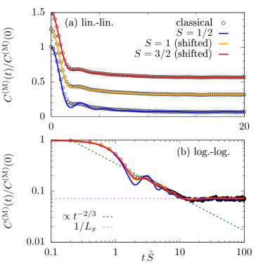
In this paper, we explore the question of quantum versus classical dynamics in spin systems by analyzing time-dependent autocorrelation functions of local densities [as defined below in Eq. (5)], which are intimately related to transport processes in these models and have been studied before, both in the classical and the quantum case Müller (1988); Gerling and Landau (1989, 1990); Bagchi (2013); Li (2019); Richter et al. (2020b); Wurtz and Polkovnikov (2020). Our main finding is exemplified in Fig. 1, which shows the temporal decay of infinite-temperature spin autocorrelation functions in isotropic Heisenberg chains with different quantum numbers and (classical). As becomes apparent from Fig. 1 (a), quantum and classical dynamics agree very well with each other on short as well as long time scales, and for all values of shown here. While the agreement is slightly better for larger , it is still convincing for , where the quantum chain is integrable whereas the classical model is not. Moreover, plotted in a double-logarithmic representation [Fig. 1 (b)], we find that the hydrodynamic power-law tail at intermediate times is well described by , which suggests superdiffusive transport within the Kardar-Parisi-Zhang (KPZ) universality class Bulchandani et al. (2021); Bertini et al. (2021); Dupont and Moore (2020); Gopalakrishnan and Vasseur (2019); Das et al. (2019b); Ljubotina et al. (2017) (for more details see Sec. IV.1.1 below).
The remarkable agreement of quantum and classical dynamics in Fig. 1 provides the starting point for the further explorations in this paper. Specifically, while Fig. 1 shows results for short chains with (which is already quite demanding for ), we particularly focus on a more in-depth comparison between and using large-scale numerical simulations of XXZ models on different lattice geometries, which range from one-dimensional (1D) chains, over quasi-1D two-leg ladders, to two-dimensional (2D) square lattices; see Fig. 2. Relying on an efficient typicality-based pure-state propagation Heitmann et al. (2020); Jin et al. (2021), we treat spin- systems with up to lattice sites and study the agreement of quantum and classical spin and energy dynamics depending on the exchange anisotropy of the XXZ model and the lattice geometry chosen. In doing so, we find a remarkably good agreement for all lattice geometries, which is best for nonintegrable quantum models in quasi-one or two dimensions, and (as already indicated in Fig. 1) still convincing for integrable quantum chains, at least in cases where transport is not ballistic due to the extensive set of conservation laws.
The rest of this paper is structured as follows. First, we introduce in Sec. II the considered models and observables in the quantum case and discuss their classical counterparts as well. Here, we also comment on the diffusive decay of equal-site autocorrelations. Then, we describe in Sec. III the numerical techniques used by us, where we focus on the concept of dynamical quantum typicality. Eventually, we present our numerical results in Sec. IV and compare classical and quantum dynamics of local magnetization and energy in different lattice geometries. We summarize and conclude in Sec. V.
II Models and Observables
II.1 Models
In this paper, we consider the anisotropic Heisenberg model (XXZ model) on a rectangular lattice with periodic boundary conditions (PBC), consisting of sites in total, where and are the lattice extension in and direction, respectively. The Hamiltonian is given by,
| (1) |
where the sum runs over all bonds of nearest-neighboring sites and . The antiferromagnetic exchange coupling constant is set to in the following. The local terms in Eq. (1) read
| (2) |
where parametrizes the anisotropy in direction and the components are spin- operators at site , which fulfill the usual commutator relations ()
| (3) |
where is the Kronecker-Delta symbol and is the antisymmetric Levi-Civita tensor. For the specific case of , these components can be expressed in terms of Pauli matrices, .
While total energy is naturally conserved, i.e., , is also invariant under rotation about the axis, i.e., the total magnetization in this direction is preserved for all ,
| (4) |
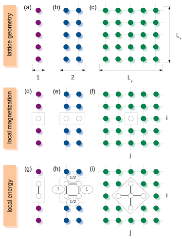
In this paper, we consider the spin- and energy-transport properties of depending on the lattice geometry, the value of , and the model being quantum or classical. In particular, we study three special cases of the lattice: (i) , i.e., a one-dimensional chain; (ii) , i.e., a quasi-1D two-leg ladder; and (iii) , i.e., a two-dimensional square lattice; see the sketch in Fig. 2. Concerning integrability, it is well known that the spin- chain is integrable in terms of the Bethe ansatz independent of the value of Bethe (1931); Levkovich-Maslyuk (2016), while integrability is broken for models with either or . This integrability will play a crucial role for our comparison of quantum and classical dynamics below. Specifically, it is well known that energy transport is purely ballistic in the integrable quantum chain, which will be in stark contrast to the dynamics of the chaotic classical chain. At the same time, integrability as such not necessarily rules out that quantum and classical transport properties can agree with each other. For instance, as demonstrated below, both the quantum and classical chain show diffusive spin transport for .
II.2 Observables
As one of the simplest quantities, we focus on the dynamics of local densities , which can be either magnetization or energy, as defined below in detail. More precisely, we consider the time-dependent density-density correlation function,
| (5) |
where with is a canonical expectation value at inverse temperature (), and the time argument of an operator has to be understood w.r.t. the Heisenberg picture, .
In the following, we discuss the equal-site autocorrelation function, i.e., in Eq. (5). Due to our choice of PBC, the autocorrelation function does not depend on the specific site and we can concisely write . Moreover, we here focus on the limit of high temperatures for which , such that is given by,
| (6) |
where is the Hilbert-space dimension, e.g., for . Note that for our numerical results, we always consider the dynamics in the full Hilbert space, i.e., we average over all sectors of fixed .
Next, we define the local densities and start with the case of magnetization. While such a definition is not unique and depends on the chosen unit cell, we use the natural definition,
| (7) |
see the sketch in Fig. 2. In the case of energy, a natural definition is,
| (8) |
for a 1D chain, i.e., just a single bond, and,
| (9) | |||||
for a quasi 1D two-leg ladder, i.e., a plaquette consisting of one bond for each leg and two rungs. Note that the factor appears, since the sum over all local energies must be identical to the total energy. For the 2D square lattice, we define,
| (10) | |||||
see the sketch in Fig. 2 again.
We note that for each local density defined above, the sum rule can be calculated analytically. For instance, in the case of local magnetization, we have for ,
| (11) |
Assuming that the system thermalizes at long times, this initial value also determines the long-time value (although there can be subtleties in some cases, see Sec. IV.2),
| (12) |
where is the total number of unit cells, i.e., in 1D or quasi-1D and in 2D. Therefore, only in the thermodynamic limit , we can expect a full decay .
II.3 Classical limit
The quantum spin models discussed so far also have a classical counterpart, which results by taking the limit of both, Planck’s constant and spin quantum number , under the constraint In this limit, the commutator relations in Eq. (3) then turn into,
| (13) |
where denotes the Poisson bracket Arnold (1978), and the spin operators become real three-dimensional vectors of constant length, . In particular, all symmetries mentioned before carry over to the classical case. The relations in Eq. (13) lead to the Hamiltonian equations of motion, which read,
| (14) |
and describe the precession of a spin around a local magnetic field resulting from the interaction with the neighboring spins. The equations (14) form a set of coupled differential equations, which is non-integrable by means of the Liouville-Arnold theorem Arnold (1978); Steinigeweg and Schmidt (2009). Therefore, they can be solved analytically only for a small number of special initial configurations, and solving them for non-trivial initial states requires numerical techniques.
The infinite-temperature density-density correlation in Eq. (6) can be obtained in the classical case by taking as an average over trajectories in phase space,
| (15) |
where the initial configurations are drawn at random for each realization , and has to be chosen sufficiently large to reduce statistical fluctuations. For the values of chosen by us, see the discussion in Sec. III.2.
In this paper, our central goal is to compare classical and quantum dynamics. Thus, for a fair comparison, we have to take into account that the sum rule is different. For instance, in the case of local magnetization, the classical sum rule is,
| (16) |
and differs from the one in Eq. (7). Thus, we always consider the rescaled data , cf. Fig. 1. Moreover, we have to rescale the time entering the quantum simulations by a factor Richter et al. (2020b),
| (17) |
in order to account for the different length of quantum and classical spins ( in the classical case). However, for , this factor is and rather close to .
II.4 Diffusion
In both, the classical and the quantum case, the time evolution of the autocorrelation function follows from the underlying microscopic equations of motion, and naturally depends on the specific model and its parameters. Thus, a precise statement on the functional form of this time evolution requires to solve the given many-body problem analytically or numerically. Due to the conservation of total energy and magnetization, however, one generally expects that the dynamics of local densities acquire a hydrodynamic behavior at sufficiently long times. In particular, in a generic nonintegrable situation, one might expect the emergence of normal diffusive transport.
In the context of the autocorrelation function , the emergence of hydrodynamics reflects itself in terms of a a power-law tail Bertini et al. (2021),
| (18) |
where normal diffusive transport corresponds to , where is the lattice dimension, i.e., in 1D or quasi-1D, and in 2D. In contrast to the case of normal diffusion, anomalous superdiffusion (cf. Fig. 1) and subdiffusion go along with an exponent and , respectively, while ballistic transport is indicated by .
Clearly, such a hydrodynamic power-law decay can only set in for times after some mean-free time . Moreover, due to the saturation at a value in any finite system, diffusion must break down for long times. Thus, in our numerical simulations below, the power-law decay in Eq. (18) can only be expected to appear in an intermediate time window, as already demonstrated in Fig. 1 above.
While the analysis of the particular type of transport for a given model and lattice geometry is not the main aspect of this paper, it naturally arises while comparing the spin and energy dynamics of quantum and classical systems in Sec. IV.
III Numerical techniques
Next, we discuss the methods used in our numerical simulations, both for the quantum and the classical case. In the former, we particularly employ the concept of dynamical quantum typicality (DQT) which gives access to autocorrelation functions for comparatively large system sizes beyond the range of full exact diagonalizaton.
III.1 Dynamical quantum typicality
DQT essentially relies on the fact that even a single pure state can imitate the full statistical ensemble. More precisely, the pure-state expectation value of an observable is typically close to the one in the statistical ensemble Lloyd (2013); Gemmer et al. (2009); Goldstein et al. (2006); Reimann (2007). This fact can be utilized to calculate the time dependence of correlation functions, e.g., the one of the density-density correlator in Eq. (5), by replacing the trace by a scalar product between two auxiliary pure states and Iitaka and Ebisuzaki (2004); Elsayed and Fine (2013); Steinigeweg et al. (2014),
| (19) |
where the two auxiliary pure states are given by,
| (20) | |||||
| (21) |
involving the reference pure state,
| (22) |
This reference pure state is drawn at random from the full Hilbert space according to the unitary invariant Haar measure Bartsch and Gemmer (2009). In practice, for any given orthogonal basis , the coefficients and are drawn randomly from a Gaussian probability distribution with zero mean.
While the statistical error in Eq. (19) depends on the specific realization of the random , the standard deviation of this statistical error can be bounded from above Jin et al. (2021),
| (23) |
where denotes an effective dimension and is the ground-state energy of . Thus, at high temperatures , and ) is negligibly small for the finite but large system sizes we are interested in. In turn, the typicality-based approximation in Eq. (19) is very accurate even for a single , and no averaging is required.
In the high-temperature limit , the correlation function can also be approximated on the basis of just one auxiliary pure state Richter and Steinigeweg (2019),
| (24) |
where is again the reference pure state in Eq. (22) and the constant is chosen in such a way that has non-negative eigenvalues. Then, the correlation function can be rewritten as a standard expectation value Richter et al. (2020b); Richter and Pal (2021); Chiaracane et al. (2021),
| (25) |
where we have employed . From a numerical point of view, Eq. (25) is more efficient than Eq. (19) as only one state has to be evolved in time. It is crucial, however, that the square root of the operator in Eq. (24) can be carried out. In the case of local magnetization, this task is trivial, at least in the Ising basis. In the case of local energy, the task also is feasible and requires only a local basis transformation, involving a few lattice sites.
The central advantage of the typicality approximations in Eqs. (19) and (25) is the fact that the time dependence appears as a property of the pure states. In particular, this time evolution can be obtained by an iterative forward propagation in real time,
| (26) |
where is a small discrete time step. Note that, even though not required for our purposes as we focus on , the action of in Eqs. (20) and (21) can be obtained by an analogous forward propagation in imaginary time Hams and De Raedt (2000).
While various sophisticated methods exist to approximate the action of the matrix exponential in Eq. (26), the massively parallelized simulations on supercomputers used by us rely on both, Trotter decompositions and Chebyshev-polynomial expansions Dobrovitski and De Raedt (2003); Weisse et al. (2006). Since the matrix-vector multiplications required in these methods can be carried out efficiently w.r.t. memory, it is possible to treat systems as large as spins, or even more Richter et al. (2019b).
III.2 Classical averaging
In the classical case, we solve the Hamiltonian equations of motion in Eq. (14) numerically by means of a fourth-order Runge-Kutta scheme (RK4), with a small time step . In particular, is chosen small enough such that the total energy and the total magnetization of are conserved to very high accuracy during the time evolution. (For other algorithms, see Ref. Krech et al., 1998.)
Since classical mechanics is not concerned with the exponential growth of the Hilbert space with system size , much larger systems can be accessed in this case. In fact, as the phase space increases only linearly with , several thousands of sites or more pose no problem. While we indeed present result for such large systems, we also consider classical chains with fewer sites to ensure a fair comparison with the quantum case.
Importantly, there is no analogue of typicality in classical mechanics. Hence, to obtain the correlation function , just a single random initial configuration is not sufficient and an average over many samples is needed instead, see Eq. (15). As a consequence, the computational cost is mainly set by and not so much by . For instance, in our numerical simulations below, we will use as many samples as , to ensure that the calculation of the correlation function goes along with small statistical errors. Note that the choice of a proper also depends on the considered time scale, i.e., a good signal-to-noise ratio at long times, where has already decayed substantially, requires a larger value of .
IV Results
We turn to the discussion of our numerical results and start in Sec. IV.1 with the dynamics of local magnetization, where we particularly compare our classical and quantum results for the different cases of 1D chains (Sec. IV.1.1), quasi-1D two-leg ladders (Sec. IV.1.2), and 2D square lattices (Sec. IV.1.2). Corresponding results for the dynamics of local energy are then presented in Sec. IV.2.
IV.1 Dynamics of local magnetization
IV.1.1 1D chain
We start with the dynamics of magnetization in a 1D chain. In Fig. 1 above, we have already presented results for the autocorrelation function at the isotropic point , where we have found that quantum dynamics for all quantum numbers agree remarkably well with the dynamics of the classical chain.
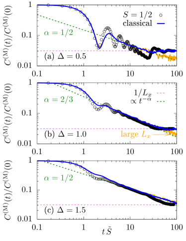
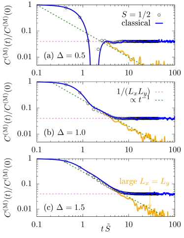
Next, we discuss the role of the anisotropy , where we focus on the comparison between the most quantum case and the classical case . Thus, compared to Fig. 1, we are able to access larger system sizes . In Fig. 3, we summarize results for for anisotropies , , and , in a double-logarithmic plot. For in Fig. 3 (b), the situation is like the one in Fig. 1 (b) discussed before. Due to the larger , the long-time saturation value becomes smaller and the power-law behavior persists on a longer time scale. Furthermore, when calculating classical data for a much larger , this range further increases. In particular, the data are still consistent with an exponent . On the one hand, in the case of the quantum chain, this superdiffusive behavior is by now well established at the isotropic point (see Ref. Bulchandani et al., 2021 and references therein). On the other hand, in the case of the classical chain, the nature of spin transport at the isotropic point has been quite controversial Müller (1988); Gerling and Landau (1989, 1990); de Alcantara Bonfim and Reiter (1992, 1993); Böhm et al. (1993); Srivastava et al. (1994). While some recent works argue that the nonintegrability eventually causes the onset of normal diffusion with when going to sufficiently large systems and long time scales Bagchi (2013); Li (2019); Dupont and Moore (2020), Ref. De Nardis et al., 2020 provides compelling arguments that the power-law tail of additionally acquires logarithmic corrections. Numerically, these scenarios are naturally very hard to distinguish.
For the larger in Fig. 3 (c), we also observe a very good agreement between quantum and classical dynamics. Compared to , the main difference is a change of the exponent from to . Hence, this value indicates a diffusive decay, which is by now well known to occur the regime , even in the case of the integrable quantum system Bertini et al. (2021). The results in Fig. 3 (b) and (c) demonstrate that integrability of the quantum model as such not necessarily prevents that its dynamics are well approximated by a simulation of a classical system instead.
For the smaller in Fig. 3 (a), we find a worse agreement between quantum and classical data, with oscillatory behavior for . While one might be tempted to conclude that the power-law decay of quantum and classical dynamics is similar at short times , such a conclusion is certainly not correct at longer times. On the one hand, as shown in Fig. 3 (a), classical dynamics for a long chain of length is diffusive with . On the other hand, quantum dynamics must be ballistic () in the thermodynamic limit, which has been proven rigorously using quasi-local conserved charges Prosen (2011); Prosen and Ilievski (2013); Ilievski et al. (2016). Thus, in such cases, where the quantum dynamics is dominated by the extensive set of conservation laws, the remarkable correspondence between quantum and classical dynamics necessarily has to break down.
IV.1.2 Quasi-1D two-leg ladder and 2D square lattice
Next, we move from 1D chains to lattice geometries of higher dimension, i.e., quasi-1D two-leg ladders and 2D square lattices. By doing so, we break the integrability of the quantum system with . This non-integrable situation is certainly more generic and might be seen as a fair test bed for the comparison between the dynamics in models with and . As before, we focus on the decay of local magnetization and consider different values of the anisotropy .
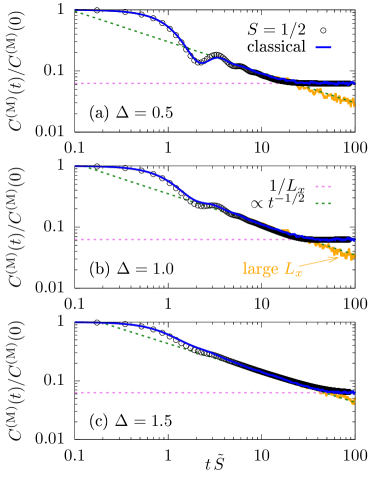
For the quasi-1D two-leg ladder, we show in Fig. 4 the equal-site correlation for , , and , where we fix the length of the ladder to . In contrast to the integrable case discussed before, we find a convincing agreement between quantum and classical relaxation for all three values of . In particular, the time dependence of at intermediate times turns out to be well described by a power law with the same diffusive exponent Richter et al. (2019b). For , this power-law behavior can be seen more clearly for larger while, for classical systems with a much larger , it becomes even more pronounced. In view of non-integrability, the qualitative similarity of quantum and classical mechanics might not be too surprising. However, it is quite remarkable that the curves in Fig. 4 agree even on a quantitative level to high accuracy.
For the 2D square lattice, we summarize in Fig. 5 the decay of for the same values of and a fixed edge length . The overall situation appears to be similar to the one for the quasi-1D two-leg ladder, e.g., the relaxation is well described by a power law with a diffusive exponent , which is in this 2D case Richter and Pal (2021). For in Fig. 5 (a), this power-law behavior cannot be seen at all for due to finite-size effects, both for the quantum and the classical system. However, when calculating classical data with a substantially larger , the diffusive decay eventually develops clearly also for .
IV.2 Dynamics of local energy
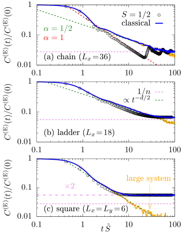
Finally, we turn to the dynamics of local energy. In this way, we want to ensure that the good agreement between quantum and classical dynamics is not restricted to the transport of local magnetization discussed above. For simplicity, let us focus on the isotropic point and study the impact of different lattice geometries.
In Fig. 6, we show the time dependence of for a 1D chain, a quasi-1D two-leg ladder, and a 2D square lattice, where we compare the dynamics of and in finite systems. For the quasi-1D and 2D cases in Fig. 6 (b) and (c), we observe a very good agreement between quantum and classical relaxation. However, for the 1D case in Fig. 6 (a), substantial differences can be clearly seen. In fact, these differences must occur as energy dynamics is ballistic () for due to integrability Zotos et al. (1997), while the classical chain exhibits diffusive energy transport instead (). Hence, Fig. 6 (a), just like Fig. 3 (a), constitutes a counterexample to our typical observation that the decay of quantum and classical density-density correlations agree qualitatively and quantitatively.
As a technical side remark, we note that the energy-energy correlation functions saturate at a long-time value which disagrees with the naive prediction in Eq. (12),
| (27) |
This fact can be seen most clearly for the 2D square lattice in Fig. 6 (c). However, this observation should not be misunderstood as a breakdown of equipartition or thermalization. In fact, the prediction for the long-time value of in Eq. (12) generally is,
| (28) |
where the reference site is fixed. We note that Eq. (28) is only identical to Eq. (12) if there is no overlap between local densities at different sites. Such overlaps occur however naturally, given the definitions of the local energies in Eqs. (8) - (10). For instance, for our choice of the local energy in 2D, the density on site shares a common bond with each of the four neighboring local energies , with , see Fig. 2 (i). Hence, these bonds contribute to Eq. (28) and give rise to a correction by a factor of , i.e.,
| (29) |
which is indicated in Fig. 6 (c) and coincides with the numerical simulation. Similar corrections apply to the long-time value of in chains and ladders as well, albeit they are less pronounced in these cases.
V Summary
In this paper, we have addressed the question whether and to which degree the dynamics in spin systems with and agree, focusing on the limit of high temperatures . We have explored this question by studying XXZ models on different lattice geometries of finite size, ranging from 1D chains, over quasi-1D two-leg ladders, to 2D square lattices. In particular, we have analyzed the temporal decay of autocorrelation functions of local spin or energy densities, which are intimately related to transport properties in these models. In order to mitigate finite-size effects, we have relied on a combination of supercomputing and the typicality-based forward propagation of pure states, which has allowed us to treat quantum systems with up to in total. As a main result, we have unveiled a remarkably good agreement between quantum and classical dynamics for all lattice geometries considered, which has been most pronounced for nonintegrable quantum systems in quasi-one or two dimensions. Still, the agreement has turned out to be satisfactory also in the integrable quantum chain, at least in cases where the quantum dynamics is not ballistic due to the presence of additional conservation laws. Based on these findings, we conclude that classical or semi-classical/hybrid simulations might provide a meaningful strategy to investigate the quantum dynamics of strongly interacting quantum spin models, even if is small and far away from the classical limit.
While the numerical advantage of such classical simulations is obvious due to the substantially larger system sizes treatable, we have yet neither a rigorous argument for the good agreement observed nor an analytical estimate for the differences remaining. On the one hand, an approximate agreement between the quantum and classical versions of might not be too surprising in cases where the quantum chain exhibits normal diffusive transport, as the emerging hydrodynamics on a coarse-grained level should be effectively describable as a classical phenomenon. On the other hand, notwithstanding these arguments, the nice agreement between and on a quantitative level, and on all time scales (even before the onset of hydrodynamics), remains remarkable to us.
Our work raises a number of questions. First, it is not clear if a similar agreement between quantum and classical dynamics is expected for other observables beyond local densities or other out-of-equilibrium quantities beyond correlation functions. Secondly, another interesting direction of research is to clarify how far this agreement carries over to finite temperatures. Yet, it is clear that there should be some low-energy scale, where the specific excitations of a given quantum model become most relevant and likely cause large differences to the classical counterpart. Eventually, it would be interesting to compare the dynamics of quantum and classical models in the presence of disorder. While strongly disordered one-dimensional quantum models are believed to undergo a many-body localization transition, such a comparison would be particulary interesting in higher dimensions, where the fate of many-body localization is less clear.
Acknowledgments
This work has been financially supported by the Deutsche Forschungsgemeinschaft (DFG), Grant No. 397067869 (STE 2243/3-1), within the DFG Research Unit FOR 2692, Grant No. 355031190. J. R. has been funded by the European Research Council (ERC) under the European Union’s Horizon 2020 research and innovation programme (Grant agreement No. 853368). Additionally, we gratefully acknowledge the computing time, granted by the “JARA-HPC Vergabegremium” and provided on the “JARA-HPC Partition” part of the supercomputer “JUWELS” at Forschungszentrum Jülich.
Appendix A Frequency space
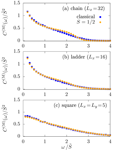
In the main text, we have focused on a comparison of quantum () and classical () mechanics in the time domain. This comparison could be done equally well in the frequency domain. Thus, in addition to the data for the correlation function presented in Sec. IV, we present here data for the corresponding spectral function , which can be obtained from the Fourier transform
| (30) |
with a finite cut-off time , yielding a frequency resolution . In Fig. 7, we exemplary depict the Fourier transform for the case of magnetization and anisotropy . We do so for the 1D, quasi-1D, and 2D lattice geometry. Apparently, the agreement between quantum and classical mechanics is very good in the frequency domain as well.
References
- Polkovnikov et al. (2011) A. Polkovnikov, K. Sengupta, A. Silva, and M. Vengalattore, Rev. Mod. Phys. 83, 863 (2011).
- Eisert et al. (2015) J. Eisert, M. Friesdorf, and C. Gogolin, Nature Phys. 11, 124 (2015).
- Mikeska and Kolezhuk (2004) H.-J. Mikeska and A. K. Kolezhuk, One-Dimensional Magnetism (Springer, 2004).
- Bloch et al. (2008) I. Bloch, J. Dalibard, and W. Zwerger, Rev. Mod. Phys. 80, 885 (2008).
- Langen et al. (2015) T. Langen, R. Geiger, and J. Schmiedmayer, Annu. Rev. Condens. Matter Phys. 6, 201 (2015).
- Smith et al. (2019) A. Smith, M. S. Kim, F. Pollmann, and J. Knolle, npj Quantum Inf. 5 (2019).
- Richter and Pal (2021) J. Richter and A. Pal, Phys. Rev. Lett. 126, 230501 (2021).
- Deutsch (1991) J. M. Deutsch, Phys. Rev. A 43, 2046 (1991).
- Srednicki (1994) M. Srednicki, Phys. Rev. E 50, 888 (1994).
- Rigol et al. (2008) M. Rigol, V. Dunjko, and M. Olshanii, Nature 452, 854 (2008).
- D’Alessio et al. (2016) L. D’Alessio, Y. Kafri, A. Polkovnikov, and M. Rigol, Adv. Phys. 65, 239 (2016).
- Borgonovi et al. (2016) F. Borgonovi, F. M. Izrailev, L. F. Santos, and V. G. Zelevinsky, Phys. Rep. 626, 1 (2016).
- Nandkishore and Huse (2015) R. Nandkishore and D. Huse, Annu. Rev. Condens. Matter Phys. 6, 15 (2015).
- Abanin et al. (2019) D. A. Abanin, E. Altman, I. Bloch, and M. Serbyn, Rev. Mod. Phys. 91, 021001 (2019).
- Prosen (2011) T. Prosen, Phys. Rev. Lett. 106, 217206 (2011).
- Prosen and Ilievski (2013) T. Prosen and E. Ilievski, Phys. Rev. Lett. 111, 057203 (2013).
- Ilievski et al. (2016) E. Ilievski, M. Medenjak, T. Prosen, and L. Zadnik, J. Stat. Mech. 2016, 064008 (2016).
- Bertini et al. (2021) B. Bertini, F. Heidrich-Meisner, C. Karrasch, T. Prosen, R. Steinigeweg, and M. Žnidarič, Rev. Mod. Phys. 93, 025003 (2021).
- Bulchandani et al. (2021) V. B. Bulchandani, S. Gopalakrishnan, and E. Ilievski, arXiv:2103.01976 (2021).
- Castro-Alvaredo et al. (2016) O. A. Castro-Alvaredo, B. Doyon, and T. Yoshimura, Phys. Rev. X 6, 041065 (2016).
- Bertini et al. (2016) B. Bertini, M. Collura, J. D. Nardis, and M. Fagotti, Phys. Rev. Lett. 117, 207201 (2016).
- Schollwöck (2005) U. Schollwöck, Rev. Mod. Phys. 77, 259 (2005).
- Schollwöck (2011) U. Schollwöck, Ann. Phys. 326, 96 (2011).
- Prelovšek and Bonča (2013) P. Prelovšek and J. Bonča, Ground State and Finite Temperature Lanczos Methods (Springer, 2013).
- Czarnik et al. (2019) P. Czarnik, J. Dziarmaga, and P. Corboz, Phys. Rev. B 99, 035115 (2019).
- Gan and Hazzard (2020) J. Gan and K. R. A. Hazzard, Phys. Rev. A 102, 013318 (2020).
- Verdel et al. (2021) R. Verdel, M. Schmitt, Y.-P. Huang, P. Karpov, and M. Heyl, Phys. Rev. B 103, 165103 (2021).
- Leviatan et al. (2017) E. Leviatan, F. Pollmann, J.H. Bardarson, D.A. Huse, and E. Altman, arXiv:1702.08894 (2017).
- Richter et al. (2020a) J. Richter, T. Heitmann, and R. Steinigeweg, SciPost Phys. 9, 31 (2020a).
- De Nicola (2021) S. De Nicola, arXiv:2103.16468 (2021).
- Dauxois (2008) T. Dauxois, Phys. Today 61, 55 (2008).
- Windsor (1967) C. G. Windsor, Proc. Phys. Soc. 91, 353 (1967).
- Lurie et al. (1974) N. A. Lurie, D. L. Huber, and M. Blume, Phys. Rev. B 9, 2171 (1974).
- Müller (1988) G. Müller, Phys. Rev. Lett. 60, 2785 (1988).
- Gerling and Landau (1989) R. W. Gerling and D. P. Landau, Phys. Rev. Lett. 63, 812 (1989).
- Gerling and Landau (1990) R. W. Gerling and D. P. Landau, Phys. Rev. B 42, 8214 (1990).
- de Alcantara Bonfim and Reiter (1992) O. F. de Alcantara Bonfim and G. Reiter, Phys. Rev. Lett. 69, 367 (1992).
- de Alcantara Bonfim and Reiter (1993) O. F. de Alcantara Bonfim and G. Reiter, Phys. Rev. Lett. 70, 249 (1993).
- Böhm et al. (1993) M. Böhm, R. W. Gerling, and H. Leschke, Phys. Rev. Lett. 70, 248 (1993).
- Srivastava et al. (1994) N. Srivastava, J.-M. Liu, V. S. Viswanath, and G. Müller, J. Appl. Phys. 75, 6751 (1994).
- Constantoudis and Theodorakopoulos (1997) V. Constantoudis and N. Theodorakopoulos, Phys. Rev. E 55, 7612 (1997).
- Oganesyan et al. (2009) V. Oganesyan, A. Pal, and D. A. Huse, Phys. Rev. B 80, 115104 (2009).
- Steinigeweg (2012) R. Steinigeweg, Europhys. Lett. 97, 67001 (2012).
- Huber (2012) D. L. Huber, Physica B 407, 4274 (2012).
- Bagchi (2013) D. Bagchi, Phys. Rev. B 87, 075133 (2013).
- Prosen and Žunkovič (2013) T. Prosen and B. Žunkovič, Phys. Rev. Lett. 111, 040602 (2013).
- Jenčič and Prelovšek (2015) B. Jenčič and P. Prelovšek, Phys. Rev. B 92, 134305 (2015).
- Das et al. (2019a) A. Das, K. Damle, A. Dhar, D. A. Huse, M. Kulkarni, C. B. Mendl, and H. Spohn, J. Stat. Phys. 180, 238 (2019a).
- Li (2019) N. Li, Phys. Rev. E 100, 062104 (2019).
- Glorioso et al. (2021) P. Glorioso, L. Delacrétaz, X. Chen, R. Nandkishore, and A. Lucas, SciPost Phys. 10 (2021).
- Lagendijk and De Raedt (1977) A. Lagendijk and H. De Raedt, Phys. Rev. B 16, 293 (1977).
- De Raedt et al. (1981) H. De Raedt, J. Fivez, and B. De Raedt, Phys. Rev. B 24, 1562 (1981).
- Steinigeweg and Schmidt (2009) R. Steinigeweg and H.-J. Schmidt, Math. Phys. Anal. Geom. 12, 19 (2009).
- Jin et al. (2013) F. Jin, T. Neuhaus, K. Michielsen, S. Miyashita, M. A. Novotny, M. I. Katsnelson, and H. De Raedt, New J. Phys. 15, 033009 (2013).
- Das et al. (2018) A. Das, S. Chakrabarty, A. Dhar, A. Kundu, D. A. Huse, R. Moessner, S. S. Ray, and S. Bhattacharjee, Phys. Rev. Lett. 121, 024101 (2018).
- Gamayun et al. (2019) O. Gamayun, Y. Miao, and E. Ilievski, Phys. Rev. B 99, 140301 (2019).
- Richter et al. (2020b) J. Richter, D. Schubert, and R. Steinigeweg, Phys. Rev. Research 2, 013130 (2020b).
- Elsayed et al. (2015b) T. A. Elsayed, and B. V. Fine, Phys. Rev. B 91, 094424 (2015b).
- Starkov et al. (2018b) G. A. Starkov, and B. V. Fine, Phys. Rev. B 98, 214421 (2018b).
- Starkov et al. (2018b) G. A. Starkov, and B. V. Fine, Phys. Rev. B 101, 024428 (2020b).
- Das et al. (2019b) A. Das, M. Kulkarni, H. Spohn, and A. Dhar, Phys. Rev. E 100, 042116 (2019b).
- de Wijn et al. (2012) A. S. de Wijn, B. Hess, and B. V. Fine, Phys. Rev. Lett. 109, 034101 (2012).
- Dupont and Moore (2020) M. Dupont and J. E. Moore, Phys. Rev. B 101, 121106 (2020).
- Richter et al. (2019a) J. Richter, N. Casper, W. Brenig, and R. Steinigeweg, Phys. Rev. B 100, 144423 (2019a).
- Ren et al. (2020) J. Ren, Q. Li, W. Li, Z. Cai, and X. Wang, Phys. Rev. Lett. 124, 130602 (2020).
- Wurtz and Polkovnikov (2020) J. Wurtz and A. Polkovnikov, Phys. Rev. E 101, 052120 (2020).
- Gopalakrishnan and Vasseur (2019) S. Gopalakrishnan and R. Vasseur, Phys. Rev. Lett. 122, 127202 (2019).
- Ljubotina et al. (2017) M. Ljubotina, M. Žnidarič, and T. Prosen, Nat. Commun. 8 (2017).
- Heitmann et al. (2020) T. Heitmann, J. Richter, D. Schubert, and R. Steinigeweg, Z. Naturforsch. A 75, 421 (2020).
- Jin et al. (2021) F. Jin, D. Willsch, M. Willsch, H. Lagemann, K. Michielsen, and H. De Raedt, J. Phys. Soc. Jpn. 90, 012001 (2021).
- Bethe (1931) H. Bethe, Z. Phys. 71, 205 (1931).
- Levkovich-Maslyuk (2016) F. Levkovich-Maslyuk, J. Phys. A Math. Theor. 49, 323004 (2016).
- Arnold (1978) V. I. Arnold, Mathematical Methods of Classical Mechanics (Springer, 1978).
- Lloyd (2013) S. Lloyd, arXiv:1307.0378 (2013).
- Gemmer et al. (2009) J. Gemmer, M. Michel, and G. Mahler, Quantum Thermodynamics (Springer, 2009).
- Goldstein et al. (2006) S. Goldstein, J. L. Lebowitz, R. Tumulka, and N. Zanghì, Phys. Rev. Lett. 96, 050403 (2006).
- Reimann (2007) P. Reimann, Phys. Rev. Lett. 99, 160404 (2007).
- Iitaka and Ebisuzaki (2004) T. Iitaka and T. Ebisuzaki, Phys. Rev. E 69, 057701 (2004).
- Elsayed and Fine (2013) T. A. Elsayed and B. V. Fine, Phys. Rev. Lett. 110, 070404 (2013).
- Steinigeweg et al. (2014) R. Steinigeweg, J. Gemmer, and W. Brenig, Phys. Rev. Lett. 112, 120601 (2014).
- Bartsch and Gemmer (2009) C. Bartsch and J. Gemmer, Phys. Rev. Lett. 102, 110403 (2009).
- Richter and Steinigeweg (2019) J. Richter and R. Steinigeweg, Phys. Rev. E 99, 012114 (2019).
- Chiaracane et al. (2021) C. Chiaracane, F. Pietracaprina, A. Purkayastha, and J. Goold, Phys. Rev. B 103, 184205 (2021).
- Hams and De Raedt (2000) A. Hams and H. De Raedt, Phys. Rev. E 62, 4365 (2000).
- Dobrovitski and De Raedt (2003) V. V. Dobrovitski and H. A. De Raedt, Phys. Rev. E 67, 056702 (2003).
- Weisse et al. (2006) A. Weisse, G. Wellein, A. Alvermann, and H. Fehske, Rev. Mod. Phys. 78, 275 (2006).
- Richter et al. (2019b) J. Richter, F. Jin, L. Knipschild, J. Herbrych, H. De Raedt, K. Michielsen, J. Gemmer, and R. Steinigeweg, Phys. Rev. B 99, 144422 (2019b).
- Krech et al. (1998) M. Krech, A. Bunker, and D. P. Landau, Comput. Phys. Commun. 111, 1 (1998).
- De Nardis et al. (2020) J. De Nardis, M. Medenjak, C. Karrasch, and E. Ilievski, Phys. Rev. Lett. 124, 210605 (2020).
- Zotos et al. (1997) X. Zotos, F. Naef, and P. Prelovsek, Phys. Rev. B 55, 11029 (1997).