An abstract theory of domain decomposition methods with coarse spaces of the GenEO family

Abstract

Two-level domain decomposition methods are preconditioned Krylov solvers. What separates one and two- level domain decomposition method is the presence of a coarse space in the latter. The abstract Schwarz framework is a formalism that allows to define and study a large variety of two-level methods. The objective of this article is to define, in the abstract Schwarz framework, a family of coarse spaces called the GenEO coarse spaces (for Generalized Eigenvalues in the Overlaps). This is a generalization of existing methods for particular choices of domain decomposition methods. Bounds for the condition numbers of the preconditioned operators are proved that are independent of the parameters in the problem (e.g., any coefficients in an underlying PDE or the number of subdomains). The coarse spaces are computed by finding low or high frequency spaces of some well chosen generalized eigenvalue problems in each subdomain.

Keywords: linear solver, domain decomposition, coarse space, preconditioning, deflation

1 Introduction

Throughout this article we consider the problem of finding $\mathbf{x}_{*}\in\mathbb{R}^{n}$ that is the solution of the following linear system

$$\mathbf{A}\mathbf{x}_{*}=\mathbf{b},\text{ where $\mathbf{A}\in\mathbb{R}^{n\times n}$ is symmetric positive and definite (spd),}$$ (1)

for a given right hand side $\mathbf{b}\in\mathbb{R}^{n}$.

The applications to bare in mind are ones for which $\mathbf{A}$ is typically sparse and the number $n$ of unknowns is very large. Hence, parallel solvers, and more specifically domain decomposition solvers, are studied. The purpose of the article is to provide unified definitions and theory for two-level domain decomposition methods with coarse spaces of the GenEO family. This is done in the abstract Schwarz framework by which it is referred to the formalism presented in Chapters 2 and 3 of the book by Toselli and Widlund [47]. This framework provides both a way of defining two-level domain decomposition preconditioners and to prove condition number bounds that involve them.

Having chosen a partition of the global computational domain into subdomains, one-level domain decomposition preconditioners are sums of inverses of some well-chosen local problems in each of the subdomains. Two-level methods have an extra ingredient that is the coarse space. Choosing the coarse space comes down to choosing an extra, low rank, problem that is shared between all subdomains and solved at every iteration of the Krylov subspace solver. A good choice of coarse space can have a huge, positive, effect on the convergence of the method. It is with the introduction of coarse spaces that domain decomposition methods became scalable. Indeed, the first coarse spaces already ensured that, for some problems, the condition number of the two-level preconditioned operators did not depend on the number of subdomains and only weakly on the number of elements in each subdomain (see e.g., [14, 30] for FETI, [11, 30] for Neumann-Neumann, and [41] or [47][Lemma 3.24] for Additive Schwarz). Robustness with respect to the coefficients in the underlying partial differential equation has always been an objective. It has long been known that the solution for some, but not all, coefficient distributions, and partitions into subdomains is to adequately choose the weights that govern how global quantities are split between subdomains. The strengths and limitations of this strategy are explored in the following articles [19, 37, 38, 39]. The literature on this topic is particularly well described in [38].

Over the past decade a consensus seems to have occurred that it is worth enlarging more significantly the coarse space if this enlargement allows to achieve robustness and scalability. One popular way of doing this is to compute the coarse space by solving generalized eigenvalue problems in the subdomains. These generalized eigenvalue problems are chosen to seek out the vectors that make convergence slow. A first group of methods was tailored to the scalar elliptic problem with a varying conductivity in the Additive Schwarz framework. Among these are the two articles [15, 16] on one hand, and [34, 35, 9] on the other. The method in this last series of articles is called the ‘DtN coarse space’ (for Dirichlet-to-Neumann). Indeed, the generalized eigenvalue problems are between a DtN operator and a weighted $L_{2}$-product on the subdomain boundary. This offers the advantage of solving generalized eigenvalue problems only on the interfaces of the subdomains although they are denser than the original operators. The proof relies on weighted Poincaré inequalities [40]. The same two groups of authors contributed, with collaborators, to the set of articles [13] and [43, 44]. This time the methods apply to a much wider range of PDEs that include the linear elasticity equations. The method in [43, 44] is called GenEO for Generalized eigenvalues in the overlaps. Indeed, the generalized eigenvalue problem can be reduced to one in the overlap between subdomains. A different version of the GenEO coarse space was proposed for FETI and BDD in [45]. The problems there are reduced to the interfaces between subdomains but the name GenEO was kept since these interfaces in some sense constitute an overlap between subdomains. The family of GenEO coarse spaces has grown since with e.g., the contributions [20] for Optimized Schwarz and [32] in the context of boundary element methods. In this article the coarse spaces will be referred to as coarse spaces of the GenEO family as their construction follows the same procedure as the two original GenEO coarse spaces: [44, 45].

The idea of solving generalized eigenvalue problems to design coarse spaces with guaranteed good convergence had in fact already been proposed, unknowingly to the authors previously mentioned. Indeed, the pioneering work [31] proposes such a technique for FETI-DP and BDDC. The authors make use of a ‘Local Indicator of the Condition Number Bound’ to fill a gap in what would be an otherwise complete full proof of boundedness for the condition number. The follow-up article [42] illustrates the efficiency of the method for BDDC in a multilevel framework and [28] (by different authors) makes the proof complete in two dimensions. It must also be noted that, as early as 1999, the authors of [3] proposed a multigrid smoothed aggregation algorithm with an enrichment technique that includes low frequency eigenmodes of the operator in the aggregate (which is like a subdomain). Thanks to this procedure any convergence rate chosen a priori can be achieved. Spectral enrichment is also at the heart of the spectral algebraic multigrid method [6].

The field of coarse spaces based on generalized eigenproblems in subdomains has been so active that it is not realistic to list all contributions here. The following list gives an overview of some methods that have been developed as well as the ones already cited: [17, 22] for Additive Schwarz, [48] for additive average Schwarz, [28, 26, 4, 25, 7, 36, 27, 49] for BDDC and/or FETI-DP where the last two references in particular present impressive large scale numerical results.

In this article, the objective is to define coarse spaces for preconditioners in the abstract Schwarz framework. Compared to the framework in [47], quite a significant generalization is made by allowing the local solvers (in each subdomain) to be non-singular. The coarse spaces are defined in order for the user to have some control over the extreme eigenvalues of the preconditioned operators, and hence over convergence. This is done by exploiting the results from the abstract Schwarz framework that allow reduce the proofs of these bounds to proving properties in the subdomains. Here, similar abstract results are proved with possibly singular local problems and with weakened assumptions that make full use of the coarse space. The amount of notation has been kept to the minimum. It is fair to mention that the article [1] proposes a setting similar to the one here. One difference is that here all abstract results are proved from scratch to fit exactly the framework that is considered.

The outline of the article is the following. In Section 2, the Abstract Schwarz framework is presented. All assumptions are clearly stated and the abstract results for the spectral bounds are proved. In Section 3, the GenEO coarse spaces are introduced and the spectral bounds for the projected and preconditioned operator are proved. More precisely, there are two sets of contributions to the coarse space. Each is obtained by solving partially a generalized eigenvalue problem in each subdomain and addresses the problem of bounding one end of the spectrum of the projected and preconditioned operator. Section 4 extends the spectral results with the GenEO coarse spaces to other two-level preconditioned operators (hybrid/balanced and additive when possible). As an illustration, Section 5 considers a two-dimensional linear elasticity problem and presents precisely the Additive Schwarz, Neumann-Neumann, and inexact Schwarz preconditioners along with their GenEO coarse spaces and the resulting spectral bounds. Numerical results are presented for each method to illustrate the behaviour predicted by the theorems.

Notation

The abbreviations spd and spsd are used to mean symmetric positive definite and symmetric positive semi-definite.

Throughout the article, the following notation is used:

• $\mathbf{{I}}$ is the identity matrix of the conforming size that is always clear in the context;

• the $\ell_{2}$, or Euclidian, inner product in $\mathbb{R}^{m}$ ($m\in\mathbb{N}$) is denoted by $\langle\cdot,\cdot\rangle$ and the induced norm by $\|\cdot\|$;

• if $\mathbf{M}\in\mathbb{R}^{m}$ ($m\in\mathbb{N}$) is an spd matrix, let $\langle\cdot,\cdot\rangle_{\mathbf{M}}$ and $\|\cdot\|_{\mathbf{M}}$ denote, respectively, the inner product and norm induced by $\mathbf{M}$. They are defined as usual by

  $$\langle\mathbf{x},\mathbf{M}\mathbf{y}\rangle=\mathbf{x}^{\top}\mathbf{M}\mathbf{y},\text{ and }\|\mathbf{x}\|_{\mathbf{M}}=\langle\mathbf{x},\mathbf{M}\mathbf{x}\rangle^{1/2},\text{ for any }\mathbf{x},\mathbf{y}\in\mathbb{R}^{m};$$

• if $\mathbf{N}\in\mathbb{R}^{m}$ ($m\in\mathbb{N}$) is an spsd matrix, let $|\cdot|_{\mathbf{N}}$ denote the semi-norm induced by $\mathbf{N}$. It is defined as usual by

  $$|\mathbf{x}|_{\mathbf{N}}=\langle\mathbf{x},\mathbf{N}\mathbf{y}\rangle^{1/2}\text{ for any }\mathbf{x}\in\mathbb{R}^{m};$$

• if $\{y_{j}\}_{j=1,\dots,J}$ is a family of $J\in\mathbb{N}$ vectors in $\mathbb{R}^{m}$ ($m\in\mathbb{N}$), the matrix whose $j$-th column is $y_{j}$ for every $j$, is denoted by

  $$[\mathbf{y}_{1}|\dots|\mathbf{y}_{m}]\in\mathbb{R}^{m\times J};$$

• if $\{a_{j}\}_{j=1,\dots,J}$ is a family of $J\in\mathbb{N}$ scalars in $\mathbb{R}$ ($m\in\mathbb{N}$), the diagonal matrix with diagonal coefficients (in order) given by $(a_{1},\dots,a_{m})$ is denoted by

  $$\text{{diag}}(a_{1},\dots,a_{m});$$

• if $\mathbf{M}$ is a matrix, $\lambda(\mathbf{M})$ is one of its eigenvalues.

2 Abstract Schwarz Framework

In this section the abstract Schwarz framework is introduced in matrix formulation. This makes sense as the linear system (1) is given directly in matrix formulation.

2.1 One-level preconditioner

Let $V=\mathbb{R}^{n}$ denote the space in which the linear system (1) is to be solved, called the global space. Let $N\in\mathbb{N}$ be the chosen number of subdomains in the first level preconditioner. Let these subdomains be denoted by $V^{s}$ for $s=1,\dots,N$, assume that they are linear subspaces of $V$, that their dimensions are denoted $n^{s}$, and that they form a cover of $V$. For each subdomain, $s=1,\dots,N$, also assume that an orthonormal basis for $V^{s}$ is available and stored in the lines of a matrix ${\mathbf{R}^{s}}\in\mathbb{R}^{n^{s}\times n}$. The requirements from this paragraph are summed up in the following assumption which is made throughout the article.

Assumption 1.

For any $s=1,\dots,N$, it holds that

$${\mathbf{R}^{s}}^{\top}\in\mathbb{R}^{n\times n^{s}};\quad\mathbf{R}^{s}{\mathbf{R}^{s}}^{\top}=\mathbf{{I}};\quad V^{s}=\operatorname{range}\left({\mathbf{R}^{s}}^{\top}\right);\text{ and }V=\mathbb{R}^{n}=\sum_{s=1}^{N}V^{s}.$$

It is not required that the spaces $V^{s}$ be pairwise disjoint. In fact, for all domain decomposition methods there is some overlap between the spaces $V^{s}$. The other ingredient in defining a one-level domain decomposition method in the abstract Schwarz framework is a family of local solvers (one per subdomain). More precisely, the following is assumed

Assumption 2.

For each $s=1,\dots,N$, assume that

$$\tilde{}\mathbf{A}^{s}\in\mathbb{R}^{n^{s}\times n^{s}}\text{is an spsd matrix, and that }{\tilde{}\mathbf{A}^{s}}\,^{\dagger}\text{ is the pseudo-inverse of $\tilde{}\mathbf{A}^{s}$}.$$

The pseudo-inverse $\mathbf{M}^{\dagger}$ of any real matrix $\mathbf{M}$ is also called the Moore-Penrose inverse of $\mathbf{M}$. Its definition and characteristics can be found, e.g., in [2] and [18][section 5.5.2]. The pseudo-inverse satisfies the following properties that we will refer back to in the proofs involving ${\tilde{}\mathbf{A}^{s}}\,^{\dagger}$:

$$\mathbf{M}^{\dagger}\mathbf{M}\mathbf{M}^{\dagger}=\mathbf{M}^{\dagger};\quad\mathbf{M}\mathbf{M}^{\dagger}\mathbf{M}=\mathbf{M};\quad\text{and}\quad\operatorname{range}(\mathbf{M}^{\dagger})=\operatorname{range}(\mathbf{M}^{\top}).$$ (2)

By symmetry, the last property is $\operatorname{range}({\tilde{}\mathbf{A}^{s}}\,^{\dagger})=\operatorname{range}(\tilde{}\mathbf{A}^{s})$.

Having chosen the set of subdomains, interpolation operators, and local solvers, the one-level abstract Schwarz preconditioner for linear system (1) is defined as:

$$\mathbf{H}:=\sum_{s=1}^{N}{\mathbf{R}^{s}}^{\top}{\tilde{}\mathbf{A}^{s}}\,^{\dagger}\mathbf{R}^{s}.$$ (3)

Although, the local solvers can be singular, it is assumed that the resulting preconditioner $\mathbf{H}$ is non-singular:

Assumption 3.

Assume that the one-level abstract Schwarz preconditioner $\mathbf{H}$ is spd.

2.2 Two-level projected and preconditioned linear system

To inject a second level into the preconditioners, a coarse space and a coarse solver must be chosen. The coarse space is the central topic of this article. It will be denoted by $V^{0}$ and the following assumption is made.

Assumption 4.

A basis for the coarse space $V^{0}$ is stored in the lines of a matrix denoted ${\mathbf{R}^{0}}$:

$$V^{0}=\operatorname{range}({\mathbf{R}^{0}}^{\top});\quad{\mathbf{R}^{0}}\in\mathbb{R}^{n^{0}\times n};\quad n^{0}=\dim(V^{0});\quad n^{0}<n.$$

The dimension of the coarse space has been denoted by $n^{0}$ and it has been assumed that $n^{0}<n$ which means that the coarse space is not the entire space $\mathbb{R}^{n}$. A solver must be chosen for the coarse space. In this article we will focus on the case where the coarse solver is the exact solver on the coarse space: $(\mathbf{R}^{0}\mathbf{A}{\mathbf{R}^{0}}^{\top})^{-1}$.

There are several ways to incorporate the coarse space into the one-level preconditioner that are presented in Section 4. In the current section and the next one, the focus will temporarily be on the projected preconditioner. A crucial role is played by the $\mathbf{A}$-orthogonal projection $\boldsymbol{\Pi}$ that is characterized by $\operatorname{ker}(\boldsymbol{\Pi})=\operatorname{range}({\mathbf{R}^{0}}^{\top})$, i.e.,

$$\boldsymbol{\Pi}:=\mathbf{{I}}-{\mathbf{R}^{0}}^{\top}(\mathbf{R}^{0}\mathbf{A}{\mathbf{R}^{0}}^{\top})^{-1}\mathbf{R}^{0}\mathbf{A},\text{ where }\mathbf{{I}}\text{ is the $n\times n$ identity matrix}.$$ (4)

Indeed, the so called coarse component $(\mathbf{{I}}-\boldsymbol{\Pi})\mathbf{x}_{*}$ of the solution can be computed explicitly as:

$$(\mathbf{{I}}-\boldsymbol{\Pi})\mathbf{x}_{*}={\mathbf{R}^{0}}^{\top}(\mathbf{R}^{0}\mathbf{A}{\mathbf{R}^{0}}^{\top})^{-1}\mathbf{R}^{0}(\mathbf{A}\mathbf{x}_{*})={\mathbf{R}^{0}}^{\top}(\mathbf{R}^{0}\mathbf{A}{\mathbf{R}^{0}}^{\top})^{-1}\mathbf{R}^{0}\mathbf{b}.$$

To solve (1), it then remains to compute $\boldsymbol{\Pi}\mathbf{x}_{*}$ satisfying

$$\mathbf{A}\boldsymbol{\Pi}\mathbf{x}_{*}=\mathbf{b}-\mathbf{A}(\mathbf{I}-\boldsymbol{\Pi})\mathbf{x}_{*}=\boldsymbol{\Pi}^{\top}\mathbf{b}\text{ or, equivalently }\mathbf{H}\mathbf{A}\boldsymbol{\Pi}\mathbf{x}_{*}=\mathbf{H}\boldsymbol{\Pi}^{\top}\mathbf{b}.$$

This is done by means of the projected (by $\boldsymbol{\Pi}$) and preconditioned (by $\mathbf{H}$) conjugate gradient algorithm (PPCG) introduced and studied in [10].

2.3 Spectral bounds in the abstract framework

It is well known [10] that the convergence of PPCG depends on the effective condition number of the projected and preconditioned operator $\mathbf{H}\mathbf{A}\boldsymbol{\Pi}$ defined by

$$\kappa=\frac{\lambda_{\max}}{\lambda_{\min}};\text{ where }\left\{\begin{array}[]{l}\lambda_{\max}\text{ is the largest eigenvalue of $\mathbf{H}\mathbf{A}\boldsymbol{\Pi}$},\\ \lambda_{\min}\text{ is the smallest eigenvalue of $\mathbf{H}\mathbf{A}\boldsymbol{\Pi}$ excluding zero.}\end{array}\right.$$

The abstract Schwarz theory presented in [47][Chapters 2 and 3] provides theoretical results that greatly simplify the problem of finding bounds for $\lambda_{\min}$ and $\lambda_{\max}$. For the bound on the largest eigenvalue the results are [47][Assumption 2.3, Assumption 2.4, Lemma 2.6, Lemma 2.10 and Theorem 2.13]. For the bound on the smallest eigenvalue, the results for the projected operator can be found in [47][Theorem 2.13 under Assumption 2.12 (that weakens Assumption 2.2 by considering only elements in $\operatorname{range}(\boldsymbol{\Pi})$)]. In this section, we state and prove very similar results with the generalization that $\tilde{}\mathbf{A}^{s}$ can be singular and with $\boldsymbol{\Pi}$ playing a more central role in the assumptions. First, we define the coloring constant as in [47][Section 2.5.1].

Definition 1 (Coloring constant).

Let $\mathcal{N}\in\mathbb{N}$ be such that there exists a set $\{\mathcal{C}_{j};\,1\leq j\leq\mathcal{N}\}$ of pairwise disjoint subsets of $\llbracket 1,N\rrbracket$ satisfying

$$\llbracket 1,N\rrbracket=\bigcup_{1\leq j\leq\mathcal{N}}\mathcal{C}_{j}\text{ and }\mathbf{R}^{s}\mathbf{A}{\mathbf{R}^{t}}^{\top}=\mathbf{0}\text{ if }s,t\in\mathcal{C}_{j}\text{ with }s\not=t\text{ for some }j.$$

One can always choose $\mathcal{N}=N$ but in general there are values of $\mathcal{N}$ that are significantly smaller than the number $N$ of subdomains. The number $\mathcal{N}$ is often referred to as the coloring constant since in can be viewed as the number of colors needed to color each subdomain in such a way that any two subdomains with the same color are orthogonal. Next, the abstract result used to bound $\lambda_{\max}$ is given and proved. Note that a difference with [47][Assumption 2.4] is that the result must be proved for vectors in $\operatorname{range}(\tilde{}\mathbf{A}^{s}\,{}^{\dagger}\mathbf{R}^{s}\boldsymbol{\Pi}^{\top})$, instead of $\operatorname{range}(\tilde{}\mathbf{A}^{s}\,{}^{\dagger}\mathbf{R}^{s})$. This subtlety is what will allow to choose the coarse space, and already appeared in [45][Lemma 2.8, Lemma 3.12] in the particular settings of BDD and FETI. Another difference, is the presence of a projection operator $\tilde{}\boldsymbol{\Pi}^{s}$ in the assumption of the lemma. This weakens the assumption as long as the kernel of $\tilde{}\mathbf{A}^{s}$ (once extended to the global space) is in the coarse space.

Lemma 1 (Upper bound for $\lambda_{\max}$).

Assume that the kernels of the local solvers $\tilde{}\mathbf{A}^{s}$ contribute to the coarse space in the sense that

$$\sum_{s=1}^{N}\mathbf{R}^{s}\,{}^{\top}\operatorname{Ker}(\tilde{}\mathbf{A}^{s})\subset V^{0},$$

and, for each $s=1,\dots,N$, let $\tilde{}\boldsymbol{\Pi}^{s}$ be the $\mathbf{A}$-orthogonal projection characterized by $\operatorname{Ker}(\tilde{}\boldsymbol{\Pi}^{s})={\mathbf{R}^{s}}^{\top}\operatorname{Ker}(\tilde{}\mathbf{A}^{s})$. Assume that there exists $\omega>0$ such that

$$\|\tilde{}\boldsymbol{\Pi}^{s}{\mathbf{R}^{s}}^{\top}\mathbf{x}^{s}\|_{\mathbf{A}}^{2}\leq\omega|\mathbf{x}^{s}|_{\tilde{}\mathbf{A}^{s}}^{2}\text{ for every }s=1,\dots,N\text{ and every }\mathbf{x}^{s}\in\operatorname{range}(\tilde{}\mathbf{A}^{s}\,{}^{\dagger}\mathbf{R}^{s}\boldsymbol{\Pi}^{\top}).$$

Then the largest eigenvalue $\lambda_{\max}$ of $\mathbf{H}\mathbf{A}\boldsymbol{\Pi}$ satisfies

$$\lambda_{\max}\leq\mathcal{N}\omega,$$

where $\mathcal{N}$ is as in Definition 1.

Proof.

Let $\mathbf{x}\in\operatorname{range}(\boldsymbol{\Pi}^{\top})$. By assumption it holds that

$$\|\tilde{}\boldsymbol{\Pi}^{s}{\mathbf{R}^{s}}^{\top}\tilde{}\mathbf{A}^{s}\,{}^{\dagger}\mathbf{R}^{s}\mathbf{x}\|_{\mathbf{A}}\leq\omega\langle\tilde{}\mathbf{A}^{s}\,{}^{\dagger}\mathbf{R}^{s}\mathbf{x},\tilde{}\mathbf{A}^{s}\tilde{}\mathbf{A}^{s}\,{}^{\dagger}\mathbf{R}^{s}\mathbf{x}\rangle,\text{ for any }s=1,\dots,N.$$

With the notation $\mathbf{H}^{s}:={\mathbf{R}^{s}}^{\top}\tilde{}\mathbf{A}^{s}\,{}^{\dagger}\mathbf{R}^{s}$, this is equivalent to

$$\|\tilde{}\boldsymbol{\Pi}^{s}\mathbf{H}^{s}\mathbf{x}\|_{\mathbf{A}}^{2}\leq\omega|\mathbf{x}|_{\mathbf{H}^{s}}^{2}.$$ (5)

We next prove the intermediary result $\|\boldsymbol{\Pi}\mathbf{H}\mathbf{x}\|_{\mathbf{A}}^{2}\leq\omega\mathcal{N}\left\|\mathbf{x}\right\|_{\mathbf{H}}^{2}$ as follows

$$\|\boldsymbol{\Pi}\mathbf{H}\mathbf{x}\|_{\mathbf{A}}^{2} =\left\|\sum_{s=1}^{N}\boldsymbol{\Pi}\mathbf{H}^{s}\mathbf{x}\right\|_{\mathbf{A}}^{2}=\left\|\sum_{j=1}^{\mathcal{N}}\sum_{s\in\mathcal{C}_{j}}\boldsymbol{\Pi}\mathbf{H}^{s}\mathbf{x}\right\|_{\mathbf{A}}^{2}\leq\left(\sum_{j=1}^{\mathcal{N}}\left\|\sum_{s\in\mathcal{C}_{j}}\boldsymbol{\Pi}\mathbf{H}^{s}\mathbf{x}\right\|_{\mathbf{A}}\right)^{2}$$

$$\leq\mathcal{N}\sum_{j=1}^{\mathcal{N}}\left\|\sum_{s\in\mathcal{C}_{j}}\boldsymbol{\Pi}\mathbf{H}^{s}\mathbf{x}\right\|_{\mathbf{A}}^{2}\leq\mathcal{N}\sum_{j=1}^{\mathcal{N}}\left\|\sum_{s\in\mathcal{C}_{j}}\tilde{}\boldsymbol{\Pi}^{s}\mathbf{H}^{s}\mathbf{x}\right\|_{\mathbf{A}}^{2}=\mathcal{N}\sum_{j=1}^{\mathcal{N}}\sum_{s\in\mathcal{C}_{j}}\left\|\tilde{}\boldsymbol{\Pi}^{s}\mathbf{H}^{s}\mathbf{x}\right\|_{\mathbf{A}}^{2}$$

$$\leq\mathcal{N}\sum_{j=1}^{\mathcal{N}}\sum_{s\in\mathcal{C}_{j}}\omega\left|\mathbf{x}\right|_{\mathbf{H}^{s}}^{2}=\mathcal{N}\sum_{s=1}^{N}\omega\left|\mathbf{x}\right|_{\mathbf{H}^{s}}^{2}=\omega\mathcal{N}\left\|\mathbf{x}\right\|_{\mathbf{H}}^{2},$$

where in the first line the sets $\mathcal{C}_{j}$ are as in Definition 1; in the second line the Cauchy-Schwarz estimate in the $\ell_{2}$-inner product, the definition of $\tilde{}\boldsymbol{\Pi}^{s}$, as well as the definition of the sets $\mathcal{C}_{j}$ are applied; and (5) is injected into the third line.

Next, we prove the bound for $\lambda_{\max}$ starting with the definition of an eigenvalue:

$$\lambda_{\max}\text{ is an eigenvalue of $\mathbf{H}\mathbf{A}\boldsymbol{\Pi}$ } \Leftrightarrow\lambda_{\max}\text{ is an eigenvalue of $\boldsymbol{\Pi}^{\top}\mathbf{A}\mathbf{H}$ }$$

$$\Leftrightarrow\,\exists\mathbf{y}\in\mathbb{R}^{n};\mathbf{y}\neq\mathbf{0}\text{ such that }\boldsymbol{\Pi}^{\top}\mathbf{A}\mathbf{H}\mathbf{y}=\lambda_{\max}\mathbf{y}.$$ (6)

Let $\mathbf{y}$ be as in (6). It is obvious that $\mathbf{y}\in\operatorname{range}(\boldsymbol{\Pi}^{\top})$. Taking the inner product of (6) by $\mathbf{H}\mathbf{y}$, and injecting the intermediary result that was just proved gives

$$\lambda_{\max}\|\mathbf{y}\|_{\mathbf{H}}^{2}=\langle\mathbf{H}\mathbf{y},\boldsymbol{\Pi}^{\top}\mathbf{A}\mathbf{H}\mathbf{y}\rangle=\|\boldsymbol{\Pi}\mathbf{H}\mathbf{y}\|_{\mathbf{A}}^{2}\leq\omega\mathcal{N}\|\mathbf{y}\|_{\mathbf{H}}^{2}.$$ (7)

The common factor $\|\mathbf{y}\|_{\mathbf{H}}^{2}$ can be cancelled because $\|\mathbf{y}\|_{\mathbf{H}}^{2}=0$ would imply $\lambda_{\max}=0$, and this is not the case since the coarse space was assumed not to be the whole of $\mathbb{R}^{n}$ in Assumption 4. ∎

The abstract Schwarz theory ([47][Theorem 2.13 under Assumption 2.12]) also provides a result for bounding the spectrum of the two-level operator from below. The result proved in the next Lemma is similar with the differences that are pointed out below the lemma.

Lemma 2 (Lower bound for $\lambda_{\min}$).

Assume that the kernels of the local solvers contribute to the coarse space in the sense that

$$\sum_{s=1}^{N}\mathbf{R}^{s}\,{}^{\top}\operatorname{Ker}(\tilde{}\mathbf{A}^{s})\subset V^{0}.$$

If, for any $\mathbf{x}\in\operatorname{range}(\boldsymbol{\Pi})$, there exist $\mathbf{z}^{1},\dots,\mathbf{z}^{n}$ such that

$$\mathbf{x}=\sum_{s=1}^{N}\boldsymbol{\Pi}\mathbf{R}^{s}\,{}^{\top}\mathbf{z}^{s}\text{ and }\sum_{s=1}^{N}\langle\mathbf{z}^{s},\tilde{}\mathbf{A}^{s}\mathbf{z}^{s}\rangle\leq C_{0}^{2}\langle\mathbf{x},\mathbf{A}\mathbf{x}\rangle\quad\text{(stable splitting of $\mathbf{x}$)},$$

then, the smallest eigenvalue $\lambda_{\min}$ of $\mathbf{H}\mathbf{A}\boldsymbol{\Pi}$, excluding zero, satisfies

$$\lambda_{\min}\geq C_{0}^{-2}.$$

The differences with [47][Theorem 2.13] are the possible singularity of $\tilde{}\mathbf{A}^{s}$, the extra presence of $\boldsymbol{\Pi}$ in the definition of a splitting, and the extra assumption on the minimal coarse space.

Proof.

Let $\mathbf{x}\in\operatorname{range}(\boldsymbol{\Pi})$ and $\{\mathbf{z}^{s}\}_{s=1,\dots,N}$ provide a stable splitting as defined in the lemma, then

$$\langle\mathbf{x},\mathbf{A}\mathbf{x}\rangle=\sum_{s=1}^{N}\langle\mathbf{x},\mathbf{A}\boldsymbol{\Pi}\mathbf{R}^{s}\,{}^{\top}\mathbf{z}^{s}\rangle=\sum_{s=1}^{N}\langle\tilde{}\mathbf{A}^{s}\,{}^{\dagger}\mathbf{R}^{s}\boldsymbol{\Pi}^{\top}\mathbf{A}\mathbf{x},\tilde{}\mathbf{A}^{s}\mathbf{z}^{s}\rangle.$$

Indeed $\tilde{}\mathbf{A}^{s}\tilde{}\mathbf{A}^{s}\,{}^{\dagger}\mathbf{R}^{s}\boldsymbol{\Pi}^{\top}=\mathbf{R}^{s}\boldsymbol{\Pi}^{\top}$ holds because of (2) and

$$\operatorname{range}(\mathbf{R}^{s}\boldsymbol{\Pi}^{\top})=\left(\operatorname{Ker}(\boldsymbol{\Pi}{\mathbf{R}^{s}}^{\top})\right)^{\perp^{\ell_{2}}}\subset\left(\operatorname{Ker}(\tilde{}\mathbf{A}^{s})\right)^{\perp^{\ell_{2}}}=\operatorname{range}(\tilde{}\mathbf{A}^{s}),$$

recalling that $\mathbf{R}^{s}\,{}^{\top}\operatorname{Ker}(\tilde{}\mathbf{A}^{s})\subset V^{0}=\operatorname{Ker}(\boldsymbol{\Pi})$. Next, the generalized Cauchy-Schwarz inequality for the semi-norm induced by $\tilde{}\mathbf{A}^{s}$, the first property in (2), the Cauchy-Schwarz inequality in the $\ell_{2}$-inner product, and the stable splitting assumption are applied in order to get

$$\langle\mathbf{x},\mathbf{A}\mathbf{x}\rangle \leq\sum_{s=1}^{N}\langle\tilde{}\mathbf{A}^{s}\,{}^{\dagger}\mathbf{R}^{s}\boldsymbol{\Pi}^{\top}\mathbf{A}\mathbf{x},\tilde{}\mathbf{A}^{s}\tilde{}\mathbf{A}^{s}\,{}^{\dagger}\mathbf{R}^{s}\boldsymbol{\Pi}^{\top}\mathbf{A}\mathbf{x}\rangle^{1/2}\langle\mathbf{z}^{s},\tilde{}\mathbf{A}^{s}\mathbf{z}^{s}\rangle^{1/2}$$

$$\leq\sum_{s=1}^{N}\langle\tilde{}\mathbf{A}^{s}\,{}^{\dagger}\mathbf{R}^{s}\boldsymbol{\Pi}^{\top}\mathbf{A}\mathbf{x},\mathbf{R}^{s}\boldsymbol{\Pi}^{\top}\mathbf{A}\mathbf{x}\rangle^{1/2}\langle\mathbf{z}^{s},\tilde{}\mathbf{A}^{s}\mathbf{z}^{s}\rangle^{1/2}$$

$$\leq\left[\sum_{s=1}^{N}\langle\tilde{}\mathbf{A}^{s}\,{}^{\dagger}\mathbf{R}^{s}\boldsymbol{\Pi}^{\top}\mathbf{A}\mathbf{x},\mathbf{R}^{s}\boldsymbol{\Pi}^{\top}\mathbf{A}\mathbf{x}\rangle\right]^{1/2}\left[\sum_{s=1}^{N}\langle\mathbf{z}^{s},\tilde{}\mathbf{A}^{s}\mathbf{z}^{s}\rangle\right]^{1/2}$$

$$\leq\langle\mathbf{x},\mathbf{A}\mathbf{H}\mathbf{A}\mathbf{x}\rangle^{1/2}C_{0}\langle\mathbf{x},\mathbf{A}\mathbf{x}\rangle^{1/2}.$$

Squaring and cancelling the common factor $\langle\mathbf{x},\mathbf{A}\mathbf{x}\rangle$ ($\neq 0$ if $\mathbf{x}\neq\mathbf{0}$) yields

$$\langle\mathbf{x},\mathbf{A}\mathbf{H}\mathbf{A}\mathbf{x}\rangle\geq C_{0}^{-2}\langle\mathbf{x},\mathbf{A}\mathbf{x}\rangle,\text{ for any }\mathbf{x}\in\operatorname{range}(\boldsymbol{\Pi}).$$ (8)

Finally, the bound for $\lambda_{\min}$ is proved starting with the definition of an eigenvalue:

$$\lambda_{\min}\text{ is an eigenvalue of $\mathbf{H}\mathbf{A}\boldsymbol{\Pi}$ } \Leftrightarrow\,\exists\mathbf{x}\in\mathbb{R}^{n};\mathbf{x}\neq\mathbf{0}\text{ such that }\mathbf{H}\mathbf{A}\boldsymbol{\Pi}\mathbf{x}=\lambda_{\min}\mathbf{x}.$$

Let $\mathbf{x}$ be such an eigenvector corresponding to eigenvalue $\lambda_{\min}$. By definition, $\lambda_{\min}\neq 0$ so $\boldsymbol{\Pi}\mathbf{x}\neq\mathbf{0}$. Taking the inner product by $\mathbf{A}\boldsymbol{\Pi}\mathbf{x}$ gives

$$\langle\boldsymbol{\Pi}\mathbf{x},\mathbf{A}\mathbf{H}\mathbf{A}\boldsymbol{\Pi}\mathbf{x}\rangle=\lambda_{\min}\langle\mathbf{A}\boldsymbol{\Pi}\mathbf{x},\mathbf{x}\rangle=\lambda_{\min}\langle\mathbf{A}\boldsymbol{\Pi}\mathbf{x},\boldsymbol{\Pi}\mathbf{x}\rangle\leq\lambda_{\min}C_{0}^{2}\langle\boldsymbol{\Pi}\mathbf{x},\mathbf{A}\mathbf{H}\mathbf{A}\boldsymbol{\Pi}\mathbf{x}\rangle,$$

where the inequality comes from (8). Cancelling the common factor $\langle\boldsymbol{\Pi}\mathbf{x},\mathbf{A}\mathbf{H}\mathbf{A}\boldsymbol{\Pi}\mathbf{x}\rangle\neq 0$, leads to the conclusion that $\lambda_{\min}C_{0}^{2}\geq 1$. ∎

3 Coarse spaces of the GenEO family

In this section, the definitions of the coarse spaces are given and the bounds on the spectrum of the resulting projected and preconditioned operator are proved. First, some general results on generalized eigenvalue problems and simultaneous diagonalization are recalled. In Definition 2, the notation $\mathbf{Y}_{L}$ and $\mathbf{Y}_{H}$ is introduced to designate bases of low or high frequency spaces (with respect to a threshold and a matrix pencil).

3.1 Definitions of $\mathbf{Y}_{L}$ and $\mathbf{Y}_{H}$

The results in this subsection are not new. They all follow quite straightforwardly from the textbook result recalled in Theorem 1. The purpose of the subsection is to introduce notation for defining the coarse spaces and outlining in the, still abstract, framework the properties that will be useful in proving the theorems in the next two subsections.

Theorem 1.

from [18][Corollary 8.7.2] Let $m\in\mathbb{N}^{*}$, let $\mathbf{M}_{\mathbf{A}}$ and $\mathbf{M}_{\mathbf{B}}$ be two matrices in $\mathbb{R}^{m\times m}$. If $\mathbf{M}_{\mathbf{A}}$ is spsd and $\mathbf{M}_{\mathbf{B}}$ is spd, then there exists a non-singular $\mathbf{Y}=[\mathbf{y}_{1}|\dots|\mathbf{y}_{m}]\in\mathbb{R}^{m\times m}$, such that

$$\mathbf{Y}^{\top}\mathbf{M}_{\mathbf{A}}\mathbf{Y}=\text{{diag}}(a_{1},\dots,a_{m}),\text{ and }\mathbf{Y}^{\top}\mathbf{M}_{\mathbf{B}}\mathbf{Y}=\text{{diag}}(b_{1},\dots,b_{m}).$$

Moreover,

$$\mathbf{M}_{\mathbf{A}}\mathbf{y}_{j}=\frac{a_{j}}{b_{j}}\mathbf{M}_{B}\mathbf{y}_{j}\text{ for }j=1,\dots,m.$$

Note that all entries $b_{j}$ in the diagonalization of $\mathbf{M}_{\mathbf{B}}$ are non-zero, because $\mathbf{M}_{B}$ is spd, so $a_{j}/b_{j}$ is always well defined in $\mathbb{R}$. A couple $(\lambda=a_{j}/b_{j};\mathbf{y}_{j})$ is called an eigenpair of the generalized eigenvalue problem $\mathbf{M}_{\mathbf{A}}\mathbf{y}=\lambda\mathbf{M}_{\mathbf{B}}\mathbf{y}$ associated with the matrix pencil $(\mathbf{M}_{\mathbf{A}},\mathbf{M}_{\mathbf{B}})$, while $a_{j}/b_{j}$ is called an eigenvalue and $\mathbf{y}_{j}$ an eigenvector.

Corollary 1.

Let $m\in\mathbb{N}^{*}$, let $\mathbf{M}_{\mathbf{A}}$ and $\mathbf{M}_{\mathbf{B}}$ be two matrices in $\mathbb{R}^{m\times m}$. If $\mathbf{M}_{\mathbf{A}}$ is spsd and $\mathbf{M}_{\mathbf{B}}$ is spd, then there exists a non-singular matrix $\mathbf{Y}\in\mathbb{R}^{m\times m}$ such that

$$\mathbf{Y}^{\top}\mathbf{M}_{\mathbf{A}}\mathbf{Y}=\text{{diag}}(\lambda_{1},\dots,\lambda_{m}),\text{ with }\lambda_{1}\leq\dots\leq\lambda_{m},\text{ and }\mathbf{Y}^{\top}\mathbf{M}_{\mathbf{B}}\mathbf{Y}=\mathbf{{I}}.$$ (9)

Moreover, denoting by $\mathbf{y}_{j}$, the $j$-th column in $\mathbf{Y}$, $(\lambda_{j},\mathbf{y}_{j})$ is an eigenpair for the matrix pencil $(\mathbf{M}_{\mathbf{A}},\mathbf{M}_{\mathbf{B}})$:

$$\mathbf{M}_{\mathbf{A}}\mathbf{y}_{j}=\lambda_{j}\mathbf{M}_{B}\mathbf{y}_{j}\text{ for }j=1,\dots,m.$$

Proof.

The assumptions in Theorem 1 hold so the results from the theorem also hold. To avoid a clash in notation, denote by $\mathbf{Y}^{\prime\prime}$ the $\mathbf{Y}$ matrix from Theorem 1. Then $\mathbf{Y}$ in this corollary is obtained by performing the two following steps. First, set $\mathbf{Y}^{\prime}=\mathbf{Y}^{\prime\prime}\text{{diag}}(b_{1}^{-1/2},\dots,b_{m}^{-1/2})$. The obtained $\mathbf{Y}^{\prime}$ is non-singular and satisfies

$${\mathbf{Y}^{\prime}}^{\top}\mathbf{M}_{\mathbf{A}}\mathbf{Y}^{\prime}=\text{{diag}}(a_{1}/b_{1},\dots,a_{m}/b_{m})\text{ and }{\mathbf{Y}^{\prime}}^{\top}\mathbf{M}_{\mathbf{B}}\mathbf{Y}^{\prime}=\mathbf{{I}}.$$

Second, sort the columns in $\mathbf{Y}^{\prime}$ in non-decreasing order of $a_{k}/b_{k}$ to obtain $\mathbf{Y}$. For $k=1,\dots,m$ (in the new ordering), set $\lambda_{k}=a_{k}/b_{k}$, and let $y_{k}$ denote the $k$-th column of $\mathbf{Y}$. $\mathbf{Y}$ is non-singular and satisfies

$$\mathbf{Y}^{\top}\mathbf{M}_{\mathbf{A}}\mathbf{Y}=\text{{diag}}(\lambda_{1},\dots,\lambda_{m}),\text{ with }\lambda_{1}\leq\dots\leq\lambda_{m},\text{ and }\mathbf{Y}^{\top}\mathbf{M}_{\mathbf{B}}\mathbf{Y}=\mathbf{{I}},$$

as well as $\mathbf{M}_{\mathbf{A}}\mathbf{y}_{k}=\lambda_{k}\mathbf{M}_{B}\mathbf{y}_{k}$ for $k=1,\dots,m$.

∎

Next, for any given threshold $\tau>0$ and suitable matrix pencil $(\mathbf{M}_{\mathbf{A}},\mathbf{M}_{\mathbf{B}})$, notation for the set of eigenvectors that correspond to eigenvalues below or above the threshold $\tau$ is introduced. These are of the utmost importance as they appear in the definitions of the GenEO coarse spaces.

Definition 2.

Let $m\in\mathbb{N}^{*}$, let $\mathbf{M}_{\mathbf{A}}\in\mathbb{R}^{m\times m}$ be an spsd matrix, let $\mathbf{M}_{\mathbf{B}}\in\mathbb{R}^{m\times m}$ be an spd matrix and let $\mathbf{Y}$ and $\{\lambda_{1},\dots,\lambda_{m}\}$ be as given by Corollary 1. For any scalar $\tau>0$, set

$$\mathbf{Y}_{L}(\tau,\mathbf{M}_{\mathbf{A}},\mathbf{M}_{\mathbf{B}}):=[\mathbf{y}_{1}|\dots|\mathbf{y}_{m_{L}}],\text{ and }\mathbf{Y}_{H}(\tau,\mathbf{M}_{\mathbf{A}},\mathbf{M}_{\mathbf{B}}):=[\mathbf{y}_{m_{L}+1}|\dots|\mathbf{y}_{m}],$$

where, $m_{L}=\min\left\{k\in\llbracket 0,m-1\rrbracket;\lambda_{k+1}\geq\tau\right\}$ if $\lambda_{m}\geq\tau$ and $m_{L}=m$ otherwise.

The matrix $\mathbf{Y}_{L}(\tau,\mathbf{M}_{\mathbf{A}},\mathbf{M}_{\mathbf{B}})$ (respectively, $\mathbf{Y}_{H}(\tau,\mathbf{M}_{\mathbf{A}},\mathbf{M}_{\mathbf{B}})$) is assembled by concatenating all $\mathbf{M}_{\mathbf{B}}$-normalized eigenvectors $\mathbf{y}$ that correspond to an eigenvalue $\lambda<\tau$ (respectively, $\lambda\geq\tau$) in the generalized eigenvalue problem $\mathbf{M}_{\mathbf{A}}\mathbf{x}=\lambda\mathbf{M}_{\mathbf{B}}\mathbf{x}$.

There are choices of $\tau$ for which $m_{L}=0$ (respectively, $m_{L}=m$). In those cases, $\mathbf{Y}_{H}(\tau,\mathbf{M}_{\mathbf{A}},\mathbf{M}_{\mathbf{B}})=\mathbf{Y}$ (respectively, $\mathbf{Y}_{L}(\tau,\mathbf{M}_{\mathbf{A}},\mathbf{M}_{\mathbf{B}})=\mathbf{Y}$) and $\mathbf{Y}_{L}(\tau,\mathbf{M}_{\mathbf{A}},\mathbf{M}_{\mathbf{B}})$ (respectively, $\mathbf{Y}_{H}(\tau,\mathbf{M}_{\mathbf{A}},\mathbf{M}_{\mathbf{B}})$) has $0$ columns. By convention, we consider the range of a matrix with $0$ columns to be the empty set. To end this section, some properties of the quantities that were just defined are proved.

Lemma 3.

Let $m\in\mathbb{N}^{*}$, let $\mathbf{M}_{\mathbf{A}}\in\mathbb{R}^{m\times m}$ be an spsd matrix, let $\mathbf{M}_{\mathbf{B}}\in\mathbb{R}^{m\times m}$ be an spd matrix, and let $\tau>0$. With the notation from Definition 2, the two following properties hold

• spectral estimates:

  $$\left\{\begin{array}[]{l}|y|_{\mathbf{M}_{\mathbf{A}}}^{2}<\tau\|y\|_{\mathbf{M}_{\mathbf{B}}}^{2}\text{ for any }\mathbf{y}\in\operatorname{range}(\mathbf{Y}_{L}(\tau,\mathbf{M}_{\mathbf{A}},\mathbf{M}_{\mathbf{B}})),\\ |y|_{\mathbf{M}_{\mathbf{A}}}^{2}\geq\tau\|y\|_{\mathbf{M}_{\mathbf{B}}}^{2}\text{ for any }\mathbf{y}\in\operatorname{range}(\mathbf{Y}_{H}(\tau,\mathbf{M}_{\mathbf{A}},\mathbf{M}_{\mathbf{B}})),\end{array}\right.$$ (10)

• conjugacy :

  $$\left\{\begin{array}[]{l}\left(\operatorname{range}(\mathbf{Y}_{L}(\tau,\mathbf{M}_{\mathbf{A}},\mathbf{M}_{\mathbf{B}}))\right)^{\perp^{\ell_{2}}}=\operatorname{range}(\mathbf{M}_{\mathbf{B}}\mathbf{Y}_{H}(\tau,\mathbf{M}_{\mathbf{A}},\mathbf{M}_{\mathbf{B}}))\\ \left(\operatorname{range}(\mathbf{Y}_{H}(\tau,\mathbf{M}_{\mathbf{A}},\mathbf{M}_{\mathbf{B}}))\right)^{\perp^{\ell_{2}}}=\operatorname{range}(\mathbf{M}_{\mathbf{B}}\mathbf{Y}_{L}(\tau,\mathbf{M}_{\mathbf{A}},\mathbf{M}_{\mathbf{B}})).\end{array}\right.$$ (11)

Proof.

Throughout the proof $\mathbf{M}_{\mathbf{A}}$, $\mathbf{M}_{\mathbf{B}}$ and $\tau$ are fixed, so the shortened notation $\mathbf{Y}_{L}=\mathbf{Y}_{L}(\tau,\mathbf{M}_{\mathbf{A}},\mathbf{M}_{\mathbf{B}})$ and $\mathbf{Y}_{H}=\mathbf{Y}_{H}(\tau,\mathbf{M}_{\mathbf{A}},\mathbf{M}_{\mathbf{B}})$ is used. Also, as in Definition 2, let $m_{L}$ be the number of columns in $\mathbf{Y}_{L}$. Corollary 1 ensures that

$$\mathbf{Y}_{L}^{\top}\mathbf{M}_{\mathbf{A}}\mathbf{Y}_{L}=\text{{diag}}(\lambda_{1},\dots,\lambda_{m_{L}})\text{ and }\mathbf{Y}_{L}^{\top}\mathbf{M}_{\mathbf{B}}\mathbf{Y}_{L}=\mathbf{{I}}.$$

Any vector in $\operatorname{range}(\mathbf{Y}_{L})$ can be written in the form ($\mathbf{Y}_{L}\boldsymbol{\alpha}$) for some $\boldsymbol{\alpha}\in\mathbb{R}^{m_{L}}$, and it holds that

$$|\mathbf{Y}_{L}\boldsymbol{\alpha}|_{\mathbf{M}_{\mathbf{A}}}^{2} =\langle\boldsymbol{\alpha},\mathbf{Y}_{L}^{\top}\mathbf{M}_{\mathbf{A}}\mathbf{Y}_{L}\boldsymbol{\alpha}\rangle=\langle\boldsymbol{\alpha},\text{{diag}}(\lambda_{1},\dots,\lambda_{m_{L}})\boldsymbol{\alpha}\rangle$$

$$\leq\lambda_{m_{L}}\langle\boldsymbol{\alpha},\boldsymbol{\alpha}\rangle=\lambda_{m_{L}}\langle\boldsymbol{\alpha},\mathbf{Y}_{L}^{\top}\mathbf{M}_{\mathbf{B}}\mathbf{Y}_{L}\boldsymbol{\alpha}\rangle=\lambda_{m_{L}}\|\mathbf{Y}_{L}\boldsymbol{\alpha}\|_{\mathbf{M}_{\mathbf{B}}}^{2}<\tau\|\mathbf{Y}_{L}\boldsymbol{\alpha}\|_{\mathbf{M}_{\mathbf{B}}}^{2}.$$

The proof of (10) for $\mathbf{Y}_{H}$ is essentially identical and is skipped here. It only remains to justify $\eqref{eq:conjugacy}$. It is obvious from (9) that $\mathbf{Y}_{L}^{\top}\mathbf{M}_{\mathbf{B}}\mathbf{Y}_{H}=\mathbf{0}$ so

$$\operatorname{range}(\mathbf{M}_{\mathbf{B}}\mathbf{Y}_{H})\subset\left(\operatorname{range}(\mathbf{Y}_{L})\right)^{\perp^{\ell_{2}}}\text{ and }\operatorname{range}(\mathbf{M}_{\mathbf{B}}\mathbf{Y}_{L})\subset\left(\operatorname{range}(\mathbf{Y}_{H})\right)^{\perp^{\ell_{2}}}.$$

The dimensional arguments

$$\dim\left((\operatorname{range}(\mathbf{Y}_{L}))^{\perp^{\ell_{2}}}\right)=\operatorname{rank}(\mathbf{M}_{\mathbf{B}}\mathbf{Y}_{H})\text{ and }\dim\left((\operatorname{range}(\mathbf{Y}_{H}))^{\perp^{\ell_{2}}}\right)=\operatorname{rank}(\mathbf{M}_{\mathbf{B}}\mathbf{Y}_{L})$$

allow to conclude for each pair of subsets that the inclusion is in fact an equality. ∎

The space spanned by the columns in $\mathbf{Y}_{L}(\tau,\mathbf{M}_{\mathbf{A}},\mathbf{M}_{\mathbf{B}})$ (respectively, $\mathbf{Y}_{H}(\tau,\mathbf{M}_{\mathbf{A}},\mathbf{M}_{\mathbf{B}})$) is the low (respectively, high) frequency space for the matrix pencil $(\mathbf{M}_{\mathbf{A}},\mathbf{M}_{\mathbf{B}})$ according to threshold $\tau$. This justifies the choice of subscripts $L$ and $H$.

3.2 A coarse space for bounding $\lambda_{\max}$

Next, one of the main results in the article is given. First, a GenEO coarse space is defined with the objective of bounding from above the eigenvalues of the projected and preconditioned operator. Then, the spectral result is stated and proved.

Definition 3 (GenEO coarse space for $\lambda_{\max}$).

Let $\tau_{\sharp}$ be chosen and define

$$V^{0}_{\sharp}(\tau_{\sharp}):=\sum_{s=1}^{N}\operatorname{range}({\mathbf{R}^{s}}^{\top}\mathbf{Y}_{L}(\tau_{\sharp},\tilde{}\mathbf{A}^{s},\mathbf{R}^{s}\mathbf{A}{\mathbf{R}^{s}}^{\top})).$$

For any $s\in\llbracket 1,N\rrbracket$, the quantity $\mathbf{Y}_{L}(\tau_{\sharp},\tilde{}\mathbf{A}^{s},\mathbf{R}^{s}\mathbf{A}{\mathbf{R}^{s}}^{\top})$ is indeed well defined following Definition 2, since $\tilde{}\mathbf{A}^{s}$ is spsd and $\mathbf{R}^{s}\mathbf{A}{\mathbf{R}^{s}}^{\top}$ is spd (as a result of ${\mathbf{R}^{s}}^{\top}$ having full rank and $\mathbf{A}$ being spd). The matrix $\mathbf{Y}_{L}(\tau_{\sharp},\tilde{}\mathbf{A}^{s},\mathbf{R}^{s}\mathbf{A}{\mathbf{R}^{s}}^{\top})$ is formed by the normalized eigenvectors corresponding to eigenvalues less than $\tau_{\sharp}$ with respect to the matrix pencil $(\tilde{}\mathbf{A}^{s},\mathbf{R}^{s}\mathbf{A}{\mathbf{R}^{s}}^{\top})$.

Theorem 2 (Bound for $\lambda_{\max}$ with the GenEO coarse space).

Under Assumptions 1, 2, 3 and 4, let $\tau_{\sharp}>0$, and let $V^{0}_{\sharp}(\tau_{\sharp})$ be as proposed in Definition 3, then the largest eigenvalue $\lambda_{\max}$ of $\mathbf{H}\mathbf{A}\boldsymbol{\Pi}$ satisfies:

$$V^{0}_{\sharp}(\tau_{\sharp})\subset V^{0}\Rightarrow\lambda_{\max}\leq\frac{\mathcal{N}}{\tau_{\sharp}},$$

where $\mathcal{N}$ is the coloring constant introduced in Definition 1.

Proof.

It is assumed that $\tau_{\sharp}>0$, so for each $s=1,\dots,N$, $\operatorname{Ker}(\tilde{}\mathbf{A}^{s})\subset\mathbf{Y}_{L}(\tau_{\sharp},\tilde{}\mathbf{A}^{s},\mathbf{R}^{s}\mathbf{A}{\mathbf{R}^{s}}^{\top})$ and

$${\mathbf{R}^{s}}^{\top}\operatorname{Ker}(\tilde{}\mathbf{A}^{s})\subset V^{0}.$$

Then, according to the result in Lemma 1, a sufficient condition for the result in the theorem is that, for any $s=1,\dots,N$,

$$\mathbf{x}^{s}\in\operatorname{range}(\tilde{}\mathbf{A}^{s}\,{}^{\dagger}\mathbf{R}^{s}\boldsymbol{\Pi}^{\top})\Rightarrow\|\tilde{}\boldsymbol{\Pi}^{s}{\mathbf{R}^{s}}^{\top}\mathbf{x}^{s}\|_{\mathbf{A}}^{2}\leq\tau_{\sharp}^{-1}{\mathcal{N}}|\mathbf{x}^{s}|_{\tilde{}\mathbf{A}^{s}}^{2}.$$ (12)

Recall that $\tilde{}\boldsymbol{\Pi}^{s}$ was defined in Lemma 1. Let $s=1,\dots,N$ be fixed and, for the length of the proof let $\mathbf{Y}_{L}=\mathbf{Y}_{L}(\tau_{\sharp},\tilde{}\mathbf{A}^{s},\mathbf{R}^{s}\mathbf{A}{\mathbf{R}^{s}}^{\top})$ and $\mathbf{Y}_{H}=\mathbf{Y}_{H}(\tau_{\sharp},\tilde{}\mathbf{A}^{s},\mathbf{R}^{s}\mathbf{A}{\mathbf{R}^{s}}^{\top})$ in order to shorten notations.

We first characterize the space $\operatorname{range}(\tilde{}\mathbf{A}^{s}\,{}^{\dagger}\mathbf{R}^{s}\boldsymbol{\Pi}^{\top})$. The assumption is that $V^{0}_{\sharp}\subset V^{0}$, so

$$V^{0}_{\sharp}\subset\operatorname{ker}(\boldsymbol{\Pi})=\left(\operatorname{range}(\boldsymbol{\Pi}^{\top})\right)^{\perp^{\ell_{2}}}$$

which implies that

$$\operatorname{range}(\mathbf{Y}_{L})\subset\left(\operatorname{range}(\mathbf{R}^{s}\boldsymbol{\Pi}^{\top})\right)^{\perp^{\ell_{2}}}$$

where the $\ell_{2}$-orthogonality is now in $\mathbb{R}^{n^{s}}$ instead of $\mathbb{R}^{n}$. Taking the orthogonal again and applying (11) from Lemma 3 yields

$$\operatorname{range}(\mathbf{R}^{s}\boldsymbol{\Pi}^{\top})\subset(\operatorname{range}(\mathbf{Y}_{L}))^{\perp^{\ell_{2}}}=(\operatorname{range}(\mathbf{R}^{s}\mathbf{A}{\mathbf{R}^{s}}^{\top}\mathbf{Y}_{H}))=(\operatorname{range}(\tilde{}\mathbf{A}^{s}\mathbf{Y}_{H})).$$

It then follows that

$$\operatorname{range}(\tilde{}\mathbf{A}^{s}\,{}^{\dagger}\mathbf{R}^{s}\boldsymbol{\Pi}^{\top})\subset\operatorname{range}\left(\tilde{}\mathbf{A}^{s}\,{}^{\dagger}\tilde{}\mathbf{A}^{s}\mathbf{Y}_{H}\right)\subset\operatorname{range}(\mathbf{Y}_{H})+\operatorname{Ker}(\tilde{}\mathbf{A}^{s}),$$

by definition of $\tilde{}\mathbf{A}^{s}\,{}^{\dagger}$.

Now, let $\mathbf{x}^{s}\in\operatorname{range}(\tilde{}\mathbf{A}^{s}\,{}^{\dagger}\mathbf{R}^{s}\boldsymbol{\Pi}^{\top})$. It has just been proved that there exists a vector $\boldsymbol{\alpha}\in\mathbb{R}^{\operatorname{rank}(\mathbf{Y}_{H})}$ and $\mathbf{z}^{s}\in\operatorname{Ker}(\tilde{}\mathbf{A}^{s})$ such that

$$\mathbf{x}^{s}=\mathbf{Y}_{H}\boldsymbol{\alpha}+\mathbf{z}^{s},$$

so $\tilde{}\boldsymbol{\Pi}^{s}{\mathbf{R}^{s}}^{\top}\mathbf{x}^{s}=\tilde{}\boldsymbol{\Pi}^{s}{\mathbf{R}^{s}}^{\top}\mathbf{Y}_{H}\boldsymbol{\alpha}$. Moreover, $\tilde{}\boldsymbol{\Pi}^{s}$ being an $\mathbf{A}$-orthogonal projection, its range is the space

$$\operatorname{range}(\tilde{}\boldsymbol{\Pi}^{s})=\left(\operatorname{Ker}(\tilde{}\boldsymbol{\Pi}^{s})\right)^{\perp^{\mathbf{A}}}=\left({\mathbf{R}^{s}}^{\top}\operatorname{Ker}(\tilde{}\mathbf{A}^{s})\right)^{\perp^{\mathbf{A}}}\supset\left(\operatorname{range}({\mathbf{R}^{s}}^{\top}\mathbf{Y}_{L})\right)^{\perp^{\mathbf{A}}}.$$

The last inclusion follows from $\operatorname{Ker}(\tilde{}\mathbf{A}^{s})\subset\operatorname{range}(\mathbf{Y}_{L})$. Another application of (11) from Lemma 3 guarantees that $(\operatorname{range}(\mathbf{Y}_{H}))^{\perp^{\ell_{2}}}=\operatorname{range}(\mathbf{R}^{s}\mathbf{A}{\mathbf{R}^{s}}^{\top}\mathbf{Y}_{L})$ so

$$\operatorname{range}({\mathbf{R}^{s}}^{\top}\mathbf{Y}_{H})\subset\left(\operatorname{range}({\mathbf{R}^{s}}^{\top}\mathbf{Y}_{L})\right)^{\perp^{\mathbf{A}}}\subset\operatorname{range}(\tilde{}\boldsymbol{\Pi}^{s}).$$

Consequently, $\tilde{}\boldsymbol{\Pi}^{s}{\mathbf{R}^{s}}^{\top}\mathbf{x}^{s}={\mathbf{R}^{s}}^{\top}\mathbf{Y}_{H}\boldsymbol{\alpha}$ and the desired estimate can finally be proved, using the second spectral estimate from (10) in Lemma 1 to get the inequality,

$$\|\tilde{}\boldsymbol{\Pi}^{s}{\mathbf{R}^{s}}^{\top}\mathbf{x}^{s}\|_{\mathbf{A}}^{2}=\|{\mathbf{R}^{s}}^{\top}\mathbf{Y}_{H}\boldsymbol{\alpha}\|_{\mathbf{A}}^{2}=\|\mathbf{Y}_{H}\boldsymbol{\alpha}\|_{\mathbf{R}^{s}\mathbf{A}{\mathbf{R}^{s}}^{\top}}^{2}\leq\tau_{\sharp}^{-1}|\mathbf{Y}_{H}\boldsymbol{\alpha}|_{\tilde{}\mathbf{A}^{s}}^{2}=\tau_{\sharp}^{-1}|\mathbf{x}^{s}|_{\tilde{}\mathbf{A}^{s}}^{2}.$$

This ends the proof. ∎

3.3 A coarse space for bounding $\lambda_{\min}$

Next, another one of the main results in the article is given. A GenEO coarse space is defined with the objective of bounding from below the eigenvalues of the projected and preconditioned operator. Then, the spectral result is stated and proved. But first, a crucial assumption that both the definition and theorem rely on is stated.

Assumption 5.

Assume that there exist a family of $N$ vectors $\mathbf{y}^{s}\in\mathbb{R}^{n^{s}}$ (for $s=1,\dots,N$), a family of N spsd matrices $\mathbf{M}^{s}\in\mathbb{R}^{n^{s}\times n^{s}}$ (for $s=1,\dots,N$), and a real number $\mathcal{N}^{\prime}>0$ such that

$$\sum_{s=1}^{N}{\mathbf{R}^{s}}^{\top}\mathbf{y}^{s}=\mathbf{x},\text{ and }\sum_{s=1}^{N}\langle\mathbf{y}^{s},\mathbf{M}^{s}\mathbf{y}^{s}\rangle\leq\mathcal{N}^{\prime}\langle\mathbf{x},\mathbf{A}\mathbf{x}\rangle,\text{ for every }\mathbf{x}\in\mathbb{R}^{n}.$$ (13)

More will be said about this assumption in the next subsection. It is not always the case that matrices $\mathbf{M}^{s}$ that fit the requirement are known.

Definition 4 (GenEO coarse space for $\lambda_{\min}$).

Let Assumption 5 hold and let $\{\mathbf{M}^{s}\}_{s=1,\dots,N}$, and $\mathcal{N}^{\prime}$ be as in the Assumption. Let $\mathbf{W}^{s}\in\mathbb{R}^{n^{s}\times\operatorname{rank}(\mathbf{M}^{s})}$ be a matrix whose columns form an $\ell_{2}$-orthonormal basis of $\operatorname{range}(\mathbf{M}^{s})$. For any given $\tau_{\flat}>0$, define

$$V^{0}_{\flat}(\tau_{\flat}):=\sum_{s=1}^{N}\mathbf{R}^{s}\,{}^{\top}\operatorname{Ker}(\tilde{}\mathbf{A}^{s})+\sum_{s=1}^{N}{\mathbf{R}^{s}}^{\top}\operatorname{Ker}(\mathbf{M}^{s})+\sum_{s=1}^{N}\operatorname{range}({\mathbf{R}^{s}}^{\top}\mathbf{W}^{s}\mathbf{Y}_{H}(\tau_{\flat},{\mathbf{W}^{s}}^{\top}\tilde{}\mathbf{A}^{s}\mathbf{W}^{s},{\mathbf{W}^{s}}^{\top}\mathbf{M}^{s}\mathbf{W}^{s})).$$

For any $s\in\llbracket 1,N\rrbracket$, the quantity $\mathbf{Y}_{H}(\tau_{\flat},{\mathbf{W}^{s}}^{\top}\tilde{}\mathbf{A}^{s}\mathbf{W}^{s},{\mathbf{W}^{s}}^{\top}\mathbf{M}^{s}\mathbf{W}^{s})$ is indeed well defined following Definition 2, since ${\mathbf{W}^{s}}^{\top}\tilde{}\mathbf{A}^{s}\mathbf{W}^{s}$ is spsd, and ${\mathbf{W}^{s}}^{\top}\mathbf{M}^{s}\mathbf{W}^{s}$ is spd. The matrix $\mathbf{Y}_{H}(\tau_{\flat},{\mathbf{W}^{s}}^{\top}\tilde{}\mathbf{A}^{s}\mathbf{W}^{s},{\mathbf{W}^{s}}^{\top}\mathbf{M}^{s}\mathbf{W}^{s})$ is formed by all the normalized eigenvectors corresponding to eigenvalues greater than or equal to $\tau_{\flat}$ with respect to the matrix pencil $({\mathbf{W}^{s}}^{\top}\tilde{}\mathbf{A}^{s}\mathbf{W}^{s},{\mathbf{W}^{s}}^{\top}\mathbf{M}^{s}\mathbf{W}^{s})$.

Remark 1.

The eigensolver SLEPc [23] provides an option for a deflation space. Setting it to $\operatorname{Ker}(\mathbf{M}^{s})$ allows to solve the eigenvalue problem that enters into the definition of $V^{0}_{\flat}$.

Theorem 3 (Bound for $\lambda_{\min}$ with the GenEO coarse space).

Under Assumptions 1, 2, 3, 4, and 5, let $V^{0}_{\flat}(\tau_{\flat})$ be as proposed in Definition 4, then the smallest eigenvalue $\lambda_{\min}$ of $\mathbf{H}\mathbf{A}\boldsymbol{\Pi}$ satisfies:

$$V^{0}_{\flat}(\tau_{\flat})\subset V^{0}\Rightarrow\lambda_{\min}>\frac{1}{\tau_{\flat}\mathcal{N}^{\prime}},$$

where $\mathcal{N}^{\prime}$ is as in Assumption 5.

Proof.

The proof consists in checking that the assumptions in Lemma 2 are satisfied. The fact that $\sum_{s=1}^{N}\mathbf{R}^{s}\,{}^{\top}\operatorname{Ker}(\tilde{}\mathbf{A}^{s})\subset V^{0}$ is explicitly assumed so it remains to prove that there exists a stable splitting of any $\mathbf{x}\in\operatorname{range}(\boldsymbol{\Pi})$ with $C_{0}^{2}=\tau_{\flat}\mathcal{N}^{\prime}$.

Let $\mathbf{x}\in\operatorname{range}(\boldsymbol{\Pi})$, it will be proved that the following components form a stable splitting of $\mathbf{x}$:

$$\mathbf{z}^{s}=\mathbf{W}^{s}\mathbf{P}^{s}{\mathbf{W}^{s}}^{\top}\mathbf{y}^{s};\text{ where }\mathbf{y}^{s}\text{ comes from Assumption~{}\ref{ass:stable-split-matrix}},$$

and $\mathbf{P}^{s}$ is the $({\mathbf{W}^{s}}^{\top}\mathbf{M}^{s}\mathbf{W}^{s})$-orthogonal projection onto $\mathbf{Y}_{L}(\tau_{\flat},{\mathbf{W}^{s}}^{\top}\tilde{}\mathbf{A}^{s}\mathbf{W}^{s},{\mathbf{W}^{s}}^{\top}\mathbf{M}^{s}\mathbf{W}^{s})$.

The first requirement is that $\sum_{s=1}^{N}\boldsymbol{\Pi}{\mathbf{R}^{s}}^{\top}\mathbf{z}^{s}=\mathbf{x}$. Let $s\in\llbracket 1,N\rrbracket$ and set $\mathbf{Y}_{L}^{s}=\mathbf{Y}_{L}(\tau_{\flat},{\mathbf{W}^{s}}^{\top}\tilde{}\mathbf{A}^{s}\mathbf{W}^{s},{\mathbf{W}^{s}}^{\top}\mathbf{M}^{s}\mathbf{W}^{s})$ for the length of the proof. With the assumption in the theorem it is sufficient to check that $\boldsymbol{\Pi}{\mathbf{R}^{s}}^{\top}\left(\mathbf{{I}}-\mathbf{W}^{s}\mathbf{P}^{s}{\mathbf{W}^{s}}^{\top}\right)\mathbf{y}^{s}=0$. We proceed as follows

$$\operatorname{range}(\mathbf{{I}}-\mathbf{W}^{s}\mathbf{P}^{s}{\mathbf{W}^{s}}^{\top}) =\left(\operatorname{Ker}(\mathbf{{I}}-\mathbf{W}^{s}{\mathbf{P}^{s}}^{\top}{\mathbf{W}^{s}}^{\top})\right)^{\perp^{\ell_{2}}}$$

$$\subset\left(\operatorname{range}(\mathbf{M}^{s}\mathbf{W}^{s}\mathbf{Y}_{L}^{s})\right)^{\perp^{\ell_{2}}},$$

since $\mathbf{W}^{s}{\mathbf{P}^{s}}^{\top}({\mathbf{W}^{s}}^{\top}\mathbf{M}^{s}\mathbf{W}^{s})\mathbf{Y}_{L}^{s}=\mathbf{W}^{s}({\mathbf{W}^{s}}^{\top}\mathbf{M}^{s}\mathbf{W}^{s}){\mathbf{P}^{s}}\mathbf{Y}_{L}^{s}=\mathbf{M}^{s}{\mathbf{W}^{s}}\mathbf{Y}_{L}^{s}$ which implies that $\operatorname{range}(\mathbf{M}^{s}\mathbf{W}^{s}\mathbf{Y}_{L}^{s})\subset\operatorname{Ker}(\mathbf{{I}}-\mathbf{W}^{s}{\mathbf{P}^{s}}^{\top}{\mathbf{W}^{s}}^{\top})$. It follows that

$$\operatorname{range}(\mathbf{{I}}-\mathbf{W}^{s}\mathbf{P}^{s}{\mathbf{W}^{s}}^{\top}) =\operatorname{Ker}({\mathbf{Y}_{L}^{s}}^{\top}{\mathbf{W}^{s}}^{\top}\mathbf{M}^{s})$$

$$=\operatorname{Ker}({\mathbf{M}^{s}})+\operatorname{range}(\mathbf{W}^{s}{\mathbf{Y}_{H}(\tau_{\flat},{\mathbf{W}^{s}}^{\top}\tilde{}\mathbf{A}^{s}\mathbf{W}^{s},{\mathbf{W}^{s}}^{\top}\mathbf{M}^{s}\mathbf{W}^{s}))})$$

$$\subset\operatorname{Ker}(\boldsymbol{\Pi}{\mathbf{R}^{s}}^{\top}),$$

where in the second step, one inclusion is easy to check with (11) from Lemma 3 and the dimensions of both spaces are equal. With this, it becomes clear that $\sum_{s=1}^{N}\boldsymbol{\Pi}{\mathbf{R}^{s}}^{\top}\mathbf{z}^{s}=\mathbf{x}$ and the stability of the splitting is proved next

$$\sum_{s=1}^{N}\langle\mathbf{z}^{s},\tilde{}\mathbf{A}^{s}\mathbf{z}^{s}\rangle =\sum_{s=1}^{N}\langle\mathbf{P}^{s}{\mathbf{W}^{s}}^{\top}\mathbf{y}^{s},({\mathbf{W}^{s}}^{\top}\tilde{}\mathbf{A}^{s}\mathbf{W}^{s})\mathbf{P}^{s}{\mathbf{W}^{s}}^{\top}\mathbf{y}^{s}\rangle$$

$$<\tau_{\flat}\sum_{s=1}^{N}\langle\mathbf{P}^{s}{\mathbf{W}^{s}}^{\top}\mathbf{y}^{s},({\mathbf{W}^{s}}^{\top}\mathbf{M}^{s}\mathbf{W}^{s})\mathbf{P}^{s}{\mathbf{W}^{s}}^{\top}\mathbf{y}^{s}\rangle\text{ (by \eqref{eq:defYLYH} in Lemma~{}\ref{lem:gevp-YLYH})}$$

$$\leq\tau_{\flat}\sum_{s=1}^{N}\langle{\mathbf{W}^{s}}^{\top}\mathbf{y}^{s},({\mathbf{W}^{s}}^{\top}\mathbf{M}^{s}\mathbf{W}^{s}){\mathbf{W}^{s}}^{\top}\mathbf{y}^{s}\rangle\text{ ($\mathbf{P}^{s}$ is a $({\mathbf{W}^{s}}^{\top}\mathbf{M}^{s}\mathbf{W}^{s})$-orthogonal projection)}$$

$$=\tau_{\flat}\sum_{s=1}^{N}\langle\mathbf{y}^{s},\mathbf{M}^{s}\mathbf{y}^{s}\rangle\text{ since }\mathbf{M}^{s}\mathbf{y}^{s}=\mathbf{M}^{s}\mathbf{W}^{s}{\mathbf{W}^{s}}^{\top}\mathbf{y}^{s}+\mathbf{M}^{s}\underbrace{(\mathbf{{I}}-\mathbf{W}^{s}{\mathbf{W}^{s}}^{\top})\mathbf{y}^{s}}_{\in\operatorname{Ker}(\mathbf{M}^{s})}$$

$$\leq\tau_{\flat}\mathcal{N}^{\prime}\langle\mathbf{x},\mathbf{A}\mathbf{x}\rangle\text{ by Assumption~{}\ref{ass:stable-split-matrix}}.$$

This concludes the proof. ∎

3.4 Some corollaries for the result on $\lambda_{\min}$

In Definition 4 of ${V^{0}_{\flat}(\tau_{\flat})}$, if $\mathbf{M}^{s}$ is non-singular then $\mathbf{W}^{s}$ can be taken equal to the identity matrix. Otherwise, the effect of $\mathbf{W}^{s}$ must be implemented when computing $V^{0}_{\flat}(\tau_{\flat})$. A way of avoiding this, if the matrices $\tilde{}\mathbf{A}^{s}$ are non-singular, is to replace ${V^{0}_{\flat}}$ by the space ${V^{0}_{\flat}}^{\prime}(\tau_{\flat})$ for which the same bound on the spectrum can be obtained, as is proved in the theorem below.

Definition 5 (Alternate $V^{0}_{\flat}(\tau_{\sharp})$ if $\tilde{}\mathbf{A}^{s}$ are non-singular).

Let Assumption 5 hold and let $\{\mathbf{M}^{s}\}_{s=1,\dots,N}$ and $\mathcal{N}^{\prime}$ be as in Assumption 5. Assume that the matrices $\tilde{}\mathbf{A}^{s}$ for $s=1,\dots,N$ are non-singular. For any given $\tau_{\flat}>0$, define

$${V^{0}_{\flat}}^{\prime}(\tau_{\flat}):=\sum_{s=1}^{N}\operatorname{range}({\mathbf{R}^{s}}^{\top}\mathbf{Y}_{L}(\tau_{\flat}^{-1},\mathbf{M}^{s},\tilde{}\mathbf{A}^{s})).$$

For any $s\in\llbracket 1,N\rrbracket$, the quantity $\mathbf{Y}_{L}(\tau_{\flat}^{-1},\mathbf{M}^{s},\tilde{}\mathbf{A}^{s})$ is indeed well defined following Definition 2, since $\mathbf{M}^{s}$ is spsd, and $\tilde{}\mathbf{A}^{s}$ is spd. Notice that for any $\tau_{\flat}>0$, $\sum_{s=1}^{N}{\mathbf{R}^{s}}^{\top}\operatorname{Ker}(\mathbf{M}^{s})\subset{V^{0}_{\flat}}^{\prime}(\tau_{\flat})$.

Theorem 4.

Let Assumptions 1, 2, 3, 4, and 5 hold. Moreover, assume that the matrices $\tilde{}\mathbf{A}^{s}$ are non-singular. Let ${V^{0}_{\flat}}^{\prime}(\tau_{\flat})$ be as proposed in Definition 4 then

$${V^{0}_{\flat}}^{\prime}(\tau_{\flat})\subset V^{0}\Rightarrow\lambda_{\min}>\frac{1}{\tau_{\flat}\mathcal{N}^{\prime}},$$

where $\mathcal{N}^{\prime}$ is as in Assumption 5.

Proof.

The proof consists in checking that the assumptions in Lemma 2 are satisfied. With non-singular $\tilde{}\mathbf{A}^{s}$ matrices, the fact that $\sum_{s=1}^{N}\mathbf{R}^{s}\,{}^{\top}\operatorname{Ker}(\tilde{}\mathbf{A}^{s})\subset V^{0}$ is trivial so it remains to prove that there exists a stable splitting of any $\mathbf{x}\in\operatorname{range}(\boldsymbol{\Pi})$ with $C_{0}^{2}=\tau_{\flat}\mathcal{N}^{\prime}$.

Let $\mathbf{x}\in\operatorname{range}(\boldsymbol{\Pi})$, it will be proved that the following components form a stable splitting of $\mathbf{x}$:

$$\mathbf{z}^{s}={\mathbf{P}^{s}}^{\prime}\mathbf{y}^{s};\text{ where }\mathbf{y}^{s}\text{ comes from Assumption~{}\ref{ass:stable-split-matrix}},$$

and ${\mathbf{P}^{s}}^{\prime}$ is the $\tilde{}\mathbf{A}^{s}$-orthogonal projection onto $\mathbf{Y}_{H}({\tau_{\flat}}^{-1},\mathbf{M}^{s},\tilde{}\mathbf{A}^{s})$. The first requirement is that $\sum_{s=1}^{N}\boldsymbol{\Pi}{\mathbf{R}^{s}}^{\top}\mathbf{z}^{s}=\mathbf{x}$. With the assumption in the theorem it is sufficient to check that $\boldsymbol{\Pi}{\mathbf{R}^{s}}^{\top}\left(\mathbf{{I}}-{\mathbf{P}^{s}}^{\prime}\right)\mathbf{y}^{s}=\mathbf{0}$. This is indeed the case since $\boldsymbol{\Pi}{\mathbf{R}^{s}}^{\top}\mathbf{Y}_{L}({\tau_{\flat}}^{-1},\mathbf{M}^{s},\tilde{}\mathbf{A}^{s})=\mathbf{0}$ and

$$\operatorname{range}(\mathbf{{I}}-{\mathbf{P}^{s}}^{\prime})=\operatorname{Ker}({\mathbf{P}^{s}}^{\prime})=\left(\mathbf{Y}_{H}({\tau_{\flat}}^{-1},\mathbf{M}^{s},\tilde{}\mathbf{A}^{s})\right)^{\perp^{\tilde{}\mathbf{A}^{s}}}=\operatorname{range}(\mathbf{Y}_{L}({\tau_{\flat}}^{-1},\mathbf{M}^{s},\tilde{}\mathbf{A}^{s})),$$

by (11) in Lemma 3.

The stability of the splitting is proved next

$$\sum_{s=1}^{N}\langle\mathbf{z}^{s},\tilde{}\mathbf{A}^{s}\mathbf{z}^{s}\rangle =\sum_{s=1}^{N}\langle{\mathbf{P}^{s}}^{\prime}\mathbf{y}^{s},\tilde{}\mathbf{A}^{s}{\mathbf{P}^{s}}^{\prime}\mathbf{y}^{s}\rangle$$

$$\leq\tau_{\flat}\sum_{s=1}^{N}\langle{\mathbf{P}^{s}}^{\prime}\mathbf{y}^{s},\mathbf{M}^{s}{\mathbf{P}^{s}}^{\prime}\mathbf{y}^{s}\rangle\text{ (by \eqref{eq:defYLYH} in Lemma~{}\ref{lem:gevp-YLYH})}$$

$$\leq\tau_{\flat}\sum_{s=1}^{N}\left[\langle{\mathbf{P}^{s}}^{\prime}\mathbf{y}^{s},\mathbf{M}^{s}{\mathbf{P}^{s}}^{\prime}\mathbf{y}^{s}\rangle+\langle(\mathbf{{I}}-{\mathbf{P}^{s}}^{\prime})\mathbf{y}^{s},\mathbf{M}^{s}(\mathbf{{I}}-{\mathbf{P}^{s}}^{\prime})\mathbf{y}^{s}\rangle\right]$$

$$\leq\tau_{\flat}\sum_{s=1}^{N}\langle\mathbf{y}^{s},\mathbf{M}^{s}\mathbf{y}^{s}\rangle\text{ (by \eqref{eq:conjugacy} in Lemma~{}\ref{lem:gevp-YLYH})}$$

$$\leq\tau_{\flat}\mathcal{N}^{\prime}\langle\mathbf{x},\mathbf{A}\mathbf{x}\rangle\text{ by Assumption~{}\ref{ass:stable-split-matrix}}.$$

This concludes the proof. ∎

Remark 2.

The connection between the eigenvalue problems in Definitions 4 and 5 is discussed in [8][Lemma 7.8]. In particular it is proved that the spaces are not in general equal. In the original GenEO article [44], the matrices $\tilde{}\mathbf{A}^{s}$ are spd (Additive Schwarz preconditioner) and the matrices $\mathbf{M}^{s}$ are only spsd. The eigenvalue problem that is solved does not involve a restriction to the range of $\mathbf{M}^{s}$ because it is of the form given in Definition 5 (with one of the matrices in the generalized eigenvalue problem restricted to the overlap).

The usual way of defining the GenEO coarse spaces is slightly less general and involves a family of matrices that form a partition of unity. Here, the partition of unity matrices are not assumed to be diagonal.

Assumption 6.

There exists a family of spd matrices $\mathbf{D}^{s}\in\mathbb{R}^{n^{s}\times n^{s}}$ for $s=1,\dots,N$ that satisfy

$$\mathbf{{I}}=\sum_{s=1}^{N}\mathbf{R}^{s}\,{}^{\top}\mathbf{D}^{s}\mathbf{R}^{s}\text{ (partition of unity; $\mathbf{{I}}$ is the $n\times n$ identity matrix)}.$$ (14)

If a family of partition of unity matrices is available, then the splitting of $\mathbf{x}$ can be chosen to be $\mathbf{x}=\sum_{s=1}^{N}{\mathbf{R}^{s}}^{\top}\mathbf{y}^{s}$ with $\mathbf{y}^{s}=\mathbf{D}^{s}\mathbf{R}^{s}\mathbf{x}$. Assumption 5 can then be rewritten in the following way.

Assumption 7.

Assume that there exist a family of $N$ matrices $\mathbf{D}^{s}\in\mathbb{R}^{n^{s}\times n^{s}}$ (for $s=1,\dots,N$) that form a partition of unity (i.e., such that Assumption 6 holds), a family of N spsd matrices $\mathbf{M}^{s}\in\mathbb{R}^{n^{s}\times n^{s}}$ (for $s=1,\dots,N$), and a real number $\mathcal{N}^{\prime}>0$ such that

$$\sum_{s=1}^{N}\langle\mathbf{D}^{s}\mathbf{R}^{s}\mathbf{x},\mathbf{M}^{s}\mathbf{D}^{s}\mathbf{R}^{s}\mathbf{x}\rangle\leq\mathcal{N}^{\prime}\langle\mathbf{x},\mathbf{A}\mathbf{x}\rangle,\text{ for every }\mathbf{x}\in\mathbb{R}^{n}.$$ (15)

Assumption 7 is less general than Assumption 5. So in all the theoretical results, it is Assumption 5 that is made without loss of generality. It is important to note that the splitting of the matrix $\mathbf{A}$ is still needed and this remains a very strong assumption. The existence of $\mathbf{D}^{s}$ and a possible choice of these matrices is guaranteed in some cases by the lemma below.

Lemma 4.

If $\left(\sum_{t=1}^{N}{\mathbf{R}^{t}}^{\top}\mathbf{R}^{t}\right)$ is a diagonal matrix, one possible choice of partition of unity matrices $\mathbf{D}^{s}$ that satisfy Assumption 6 is, for any $s=1,\dots,N$, to set

$$\mathbf{D}^{s}:=\mathbf{R}^{s}\left(\sum_{t=1}^{N}{\mathbf{R}^{t}}^{\top}\mathbf{R}^{t}\right)^{-1}{\mathbf{R}^{s}}^{\top}.$$

Proof.

We first justify the fact that the inversion in the definition of $\mathbf{D}^{s}$ is well defined by proving the definiteness of the spsd matrix that is inverted. Let $\mathbf{x}\in\mathbb{R}^{n}$, the following equivalences hold

$$\langle\mathbf{x},\sum_{s=1}^{N}{\mathbf{R}^{s}}^{\top}\mathbf{R}^{s}\mathbf{x}\rangle=0\,\Leftrightarrow\,\sum_{s=1}^{N}\langle\mathbf{R}^{s}\mathbf{x},\mathbf{R}^{s}\mathbf{x}\rangle=0\,\Leftrightarrow\mathbf{x}\in\bigcap_{s=1,\dots,N}\left(\operatorname{Ker}(\mathbf{R}^{s})\right).$$

Next, we use some basic linear algebra identities and (in the last step) the assumption that $\sum_{s=1}^{N}\operatorname{range}({\mathbf{R}^{s}}^{\top})=\mathbb{R}^{n}$ to conclude that $\mathbf{x}=\mathbf{0}$:

$$\mathbf{x}\in\bigcap_{s=1,\dots,N}\left(\operatorname{Ker}(\mathbf{R}^{s})\right)=\bigcap_{s=1,\dots,N}\left(\operatorname{range}({\mathbf{R}^{s}}^{\top})\right)^{\perp^{\ell_{2}}}=\left(\sum_{s=1}^{N}\operatorname{range}({\mathbf{R}^{s}}^{\top})\right)^{\perp^{\ell_{2}}}=\{\mathbf{0}\}.$$

It may now be written that

$$\mathbf{{I}}=\sum_{s=1}^{N}\left(\sum_{t=1}^{N}{\mathbf{R}^{t}}^{\top}\mathbf{R}^{t}\right)^{-1}{\mathbf{R}^{s}}^{\top}\mathbf{R}^{s}=\sum_{s=1}^{N}{\mathbf{R}^{s}}^{\top}\mathbf{R}^{s}\left(\sum_{t=1}^{N}{\mathbf{R}^{t}}^{\top}\mathbf{R}^{t}\right)^{-1}{\mathbf{R}^{s}}^{\top}\mathbf{R}^{s}.$$

The justification for the last equality is that ${\mathbf{R}^{s}}^{\top}\mathbf{R}^{s}$ is a projection onto $\operatorname{range}\left({\mathbf{R}^{s}}^{\top}\right)$ (because the columns in ${\mathbf{R}^{s}}^{\top}$ are orthonormal) and that $\operatorname{range}\left(\left(\sum_{t=1}^{N}{\mathbf{R}^{t}}^{\top}\mathbf{R}^{t}\right)^{-1}{\mathbf{R}^{s}}^{\top}\right)=\operatorname{range}\left({\mathbf{R}^{s}}^{\top}\right)$ (because the inverted matrix is assumed to be diagonal). ∎

4 Spectral bounds with the GenEO coarse spaces

For clarity of presentation, it is recalled that the one-level preconditioner and coarse projector were defined in (3) and (4) as

$$\mathbf{H}=\sum_{s=1}^{N}{\mathbf{R}^{s}}^{\top}{\tilde{}\mathbf{A}^{s}}\,^{\dagger}\mathbf{R}^{s},\text{ and }\boldsymbol{\Pi}=\mathbf{{I}}-{\mathbf{R}^{0}}^{\top}(\mathbf{R}^{0}\mathbf{A}{\mathbf{R}^{0}}^{\top})^{-1}\mathbf{R}^{0}\mathbf{A}.$$

So far, the focus has been on the projected and preconditioned operator $\mathbf{H}\mathbf{A}\boldsymbol{\Pi}$. In this section, two other two-level preconditioners are studied: the Hybrid preconditioner and the Additive preconditioner.

Remark 3.

All the results that guarantee a lower bound for a preconditioned operator rely on the Assumption that $V^{0}_{\flat}(\tau_{\flat})\subset V^{0}$ for some $\tau_{\flat}>0$ where $V^{0}_{\flat}(\tau_{\flat})$ is from Definition 4. In the case where the matrices $\tilde{}\mathbf{A}^{s}$ are non-singular for every $s=1,\dots,N$, all results remain true with ${V^{0}_{\flat}}^{\prime}(\tau_{\flat})$ from Definition 5 instead of $V^{0}_{\flat}(\tau_{\flat})$ . To prove it, it suffices to apply Theorem 4 instead of Theorem 3 in the proofs. This will not be recalled every time a result is established.

4.1 Hybrid Schwarz with the GenEO coarse space

The Hybrid Schwarz preconditioner is defined next. It is a two-level preconditioner where the coarse space is balanced (see [46, 29, 47]).

Definition 6 (Hybrid Schwarz Preconditioner).

Under Assumptions 1, 2, and 4, the hybrid Schwarz preconditioner is defined as

$$\mathbf{H}_{hyb}:=\boldsymbol{\Pi}\mathbf{H}\boldsymbol{\Pi}^{\top}+{\mathbf{R}^{0}}^{\top}(\mathbf{R}^{0}\mathbf{A}{\mathbf{R}^{0}}^{\top})^{-1}\mathbf{R}^{0},$$

where $\mathbf{H}$ is the one-level preconditioner and $\boldsymbol{\Pi}$ is the $\mathbf{A}$-orthogonal projection satisfying $\operatorname{Ker}(\boldsymbol{\Pi})=V^{0}=\operatorname{range}({\mathbf{R}^{0}}^{\top})$ (the coarse space).

Theorem 5.

Let Assumptions 1, 2, 3, 4, and 5 hold. Let $\lambda_{\min}^{\text{target}}>0$ and $\lambda_{\max}^{\text{target}}>0$ be the desired bounds for the two-level preconditioned operator. Let the coarse space $V^{0}$ be defined as

$$V^{0}=V^{0}_{\sharp}\left(\frac{\mathcal{N}}{\lambda_{\text{max}}^{\text{target}}}\right)+V^{0}_{\flat}\left(\frac{1}{\mathcal{N}^{\prime}\lambda_{\text{min}}^{\text{target}}}\right),$$

where $V^{0}_{\sharp}$ and $V^{0}_{\flat}$ are as introduced in Definitions 3 and 4, $\mathcal{N}$ is the coloring constant from Definition 1, and $\mathcal{N}^{\prime}$ comes from Assumption 5.

Then, the eigenvalues of the projected (also called deflated) and preconditioned operator satisfy

$$\lambda(\mathbf{H}\mathbf{A}\boldsymbol{\Pi})\in\{0\}\cup[\lambda_{\min}^{\text{target}},\lambda_{\max}^{\text{target}}],\text{ and $V^{0}$ is exactly the eigenspace corresponding to $\lambda(\mathbf{H}\mathbf{A}\boldsymbol{\Pi})=0$}.$$

Moreover, the eigenvalues of the operator preconditioned by $\mathbf{H}_{hyb}$ from Definition 6 satisfy

$$\lambda(\mathbf{H}_{hyb}\mathbf{A})\in[\min(1,\lambda_{\min}^{\text{target}}),\max(1,\lambda_{\max}^{\text{target}})].$$

Proof.

The result $\lambda(\mathbf{H}\mathbf{A}\boldsymbol{\Pi})\in\{0\}\cup[\lambda_{\min}^{\text{target}},\lambda_{\max}^{\text{target}}]$ for the projected preconditioner is obtained by applying theorems 2 and 3 with $\tau_{\sharp}=\frac{\mathcal{N}}{\lambda_{\text{max}}^{\text{target}}}$ and $\tau_{\flat}=\frac{1}{\mathcal{N}^{\prime}\lambda_{\text{min}}^{\text{target}}}$. This ensures that all non-zero eigenvalues of $\mathbf{H}\mathbf{A}\boldsymbol{\Pi}$ are in the interval $[\lambda_{\min}^{\text{target}},\lambda_{\max}^{\text{target}}]$. Moreover, since $\mathbf{H}$ and $\mathbf{A}$ are non-singular, $\mathbf{H}\mathbf{A}\boldsymbol{\Pi}\mathbf{x}=\mathbf{0}$ if and only if $\mathbf{x}\in\operatorname{Ker}(\boldsymbol{\Pi})=V^{0}$ and so the eigenspace corresponding to eigenvalue $0$ is $V^{0}$.

The connection between the spectra of the projected and hybrid/balanced preconditioned operators is well known (see e.g., [46, 29]) and easy to verify. Let $\mathbf{x}\in V$, it holds that

$$\langle\mathbf{x},\mathbf{A}\mathbf{H}_{hyb}\mathbf{A}\mathbf{x}\rangle =\langle\mathbf{x},\mathbf{A}\boldsymbol{\Pi}\mathbf{H}\boldsymbol{\Pi}^{\top}\mathbf{A}\mathbf{x}\rangle+\langle\mathbf{x},\mathbf{A}{\mathbf{R}^{0}}^{\top}(\mathbf{R}^{0}\mathbf{A}{\mathbf{R}^{0}}^{\top})^{-1}\mathbf{R}^{0}\mathbf{A}\mathbf{x}\rangle$$

$$=\langle\boldsymbol{\Pi}\mathbf{x},\mathbf{A}\mathbf{H}\mathbf{A}\boldsymbol{\Pi}\mathbf{x}\rangle+\langle(\mathbf{{I}}-\boldsymbol{\Pi})\mathbf{x},\mathbf{A}(\mathbf{{I}}-\boldsymbol{\Pi})\mathbf{x}\rangle,$$

so, with the result for the projected preconditioned operator:

$$\left\{\begin{array}[]{rc}&\langle\mathbf{x},\mathbf{A}\mathbf{H}_{hyb}\mathbf{A}\rangle\geq\lambda_{\text{min}}^{\text{target}}\langle\boldsymbol{\Pi}\mathbf{x},\mathbf{A}\boldsymbol{\Pi}\mathbf{x}\rangle+\langle(\mathbf{{I}}-\boldsymbol{\Pi})\mathbf{x},\mathbf{A}(\mathbf{{I}}-\boldsymbol{\Pi})\mathbf{x}\rangle\\ \text{and }&\langle\mathbf{x},\mathbf{A}\mathbf{H}_{hyb}\mathbf{A}\rangle\leq\lambda_{\text{max}}^{\text{target}}\langle\boldsymbol{\Pi}\mathbf{x},\mathbf{A}\boldsymbol{\Pi}\mathbf{x}\rangle+\langle(\mathbf{{I}}-\boldsymbol{\Pi})\mathbf{x},\mathbf{A}(\mathbf{{I}}-\boldsymbol{\Pi})\mathbf{x}\rangle\end{array}\right.$$

and the result follows by recalling that $\boldsymbol{\Pi}$ is an $\mathbf{A}$-orthogonal projection. ∎

Corollary 2.

Let Assumptions 1, 2, 3, 4, and 5 hold. Let $\tau_{\sharp}>0$ and $\tau_{\flat}>0$ and let the coarse space $V^{0}$ be defined as

$$V^{0}=V^{0}_{\sharp}\left(\tau_{\sharp}\right)+V^{0}_{\flat}\left(\tau_{\flat}\right),$$

where $V^{0}_{\sharp}(\tau_{\sharp})$ and $V^{0}_{\flat}(\tau_{\flat})$ are as introduced in Definitions 3 and 4. Then, the eigenvalues of the two-level preconditioned operators satisfy

• $\lambda(\mathbf{H}\mathbf{A}\boldsymbol{\Pi})\in\{0\}\cup[\frac{1}{\mathcal{N}^{\prime}\tau_{\flat}},\frac{\mathcal{N}}{\tau_{\sharp}}],\text{ and $V^{0}$ is exactly the eigenspace corresponding to $\lambda(\mathbf{H}\mathbf{A}\boldsymbol{\Pi})=0$}$,

• $\lambda(\mathbf{H}_{hyb}\mathbf{A})\in[\min(1,\frac{1}{\mathcal{N}^{\prime}\tau_{\flat}}),\max(1,\frac{\mathcal{N}}{\tau_{\sharp}})]$,

where again $\mathcal{N}$ is the coloring constant from Definition 1 and $\mathcal{N}^{\prime}$ comes from Assumption 5.

Proof.

Apply the previous theorem with the change of variables : $\tau_{\sharp}=\frac{\mathcal{N}}{\lambda_{\text{max}}^{\text{target}}}$ and $\tau_{\flat}=\frac{1}{\mathcal{N}^{\prime}\lambda_{\text{min}}^{\text{target}}}$ ∎

In the next corollary, it is assumed that the local solvers satisfy a stability (with constant $C_{\#}$) estimate with respect to the exact local solver $\mathbf{R}^{s}\mathbf{A}{\mathbf{R}^{s}}^{\top}$. Then a certain upper bound for the eigenvalues (that involves $C_{\#}$) holds as long as the kernels of the local operators contribute to the coarse space. In particular, it is not necessary to solve any eigenvalue problem to obtain this bound. The reason it is natural and important to consider this case is that a very frequently used preconditioner is the Additive Schwarz preconditioner where $\tilde{}\mathbf{A}^{s}=\mathbf{R}^{s}\mathbf{A}{\mathbf{R}^{s}}^{\top}$ and $C_{\#}=1$ (see Section 5.2.2).

Corollary 3.

Let Assumptions 1, 2, 3, 4, and 5 hold. Let $C_{\sharp}>0$ and assume that, for every $s=1,\dots,N$ and every $\mathbf{x}^{s}\in\mathbb{R}^{n^{s}}$,

$$\|\tilde{}\boldsymbol{\Pi}^{s}{\mathbf{R}^{s}}^{\top}\mathbf{x}^{s}\|_{\mathbf{A}}^{2}\leq C_{\sharp}^{-1}|\mathbf{x}^{s}|_{\tilde{}\mathbf{A}^{s}}^{2},$$

where, again, $\tilde{}\boldsymbol{\Pi}^{s}$ is the $\mathbf{A}$-orthogonal projection characterized by $\operatorname{Ker}(\tilde{}\boldsymbol{\Pi}^{s})={\mathbf{R}^{s}}^{\top}\operatorname{Ker}(\tilde{}\mathbf{A}^{s})$. Then,

$$\mathbf{Y}_{L}(C_{\sharp},\tilde{}\mathbf{A}^{s},\mathbf{R}^{s}\mathbf{A}{\mathbf{R}^{s}}^{\top})=\operatorname{Ker}(\tilde{}\mathbf{A}^{s}).$$

Consequently, if $\sum_{s=1}^{N}{\mathbf{R}^{s}}^{\top}\operatorname{Ker}(\tilde{}\mathbf{A}^{s})\subset V^{0}$, then the eigenvalues of the projected and hybrid preconditioned operators can be bounded from above as follows:

• $\lambda(\mathbf{H}\mathbf{A}\boldsymbol{\Pi})\leq\frac{\mathcal{N}}{C_{\sharp}},$

• $\lambda(\mathbf{H}_{hyb}\mathbf{A})\leq\max\left(1,\frac{\mathcal{N}}{C_{\sharp}}\right)$.

Moreover, for any $\tau_{\flat}>0$, if $V^{0}_{\flat}(\tau_{\flat})\subset V^{0}$, then the eigenvalues of the projected and hybrid preconditioned operators can be bounded as follows:

• $\lambda(\mathbf{H}\mathbf{A}\boldsymbol{\Pi})\in\{0\}\cup[\frac{1}{\mathcal{N}^{\prime}\tau_{\flat}},\frac{\mathcal{N}}{C_{\sharp}}],\text{ and $V^{0}$ is exactly the eigenspace corresponding to $\lambda(\mathbf{H}\mathbf{A}\boldsymbol{\Pi})=0$}$,

• $\lambda(\mathbf{H}_{hyb}\mathbf{A})\in[\min(1,\frac{1}{\mathcal{N}^{\prime}\tau_{\flat}}),\max(1,\frac{\mathcal{N}}{C_{\sharp}})]$,

where again $\mathcal{N}$ is the coloring constant from Definition 1 and $\mathcal{N}^{\prime}$ comes from Assumption 5.

Proof.

Let $s\in\llbracket 1,N\rrbracket$. It must first be proved that $\mathbf{Y}_{L}(C_{\sharp},\tilde{}\mathbf{A}^{s},\mathbf{R}^{s}\mathbf{A}{\mathbf{R}^{s}}^{\top})=\operatorname{Ker}(\tilde{}\mathbf{A}^{s})$. Since $C_{\sharp}>0$, and the vectors in $\operatorname{Ker}(\tilde{}\mathbf{A}^{s})$ form the eigenspace associated with eigenvalue $0$ with respect to the matrix pencil $(\tilde{}\mathbf{A}^{s},\mathbf{R}^{s}\mathbf{A}{\mathbf{R}^{s}}^{\top})$, it is clear that $\operatorname{Ker}(\tilde{}\mathbf{A}^{s})\subset\mathbf{Y}_{L}(C_{\sharp},\tilde{}\mathbf{A}^{s},\mathbf{R}^{s}\mathbf{A}{\mathbf{R}^{s}}^{\top})$. It remains to prove that all non-zero eigenvalues are greater than $C_{\sharp}$. Let $(\lambda^{s},\mathbf{p}^{s})\in\mathbb{R}^{*}\times\mathbb{R}^{n^{s}}$ be an eigenpair for the matrix pencil $(\tilde{}\mathbf{A}^{s},\mathbf{R}^{s}\mathbf{A}{\mathbf{R}^{s}}^{\top})$:

$$\tilde{}\mathbf{A}^{s}\mathbf{p}^{s}=\lambda^{s}\mathbf{R}^{s}\mathbf{A}{\mathbf{R}^{s}}^{\top}\mathbf{p}^{s}\text{ and }\mathbf{p}^{s}\neq\mathbf{0}\Rightarrow|\mathbf{p}^{s}|_{\tilde{}\mathbf{A}^{s}}=\lambda^{s}\|\mathbf{p}^{s}\|_{\mathbf{R}^{s}\mathbf{A}{\mathbf{R}^{s}}^{\top}}\text{ and }\|\mathbf{p}^{s}\|_{\mathbf{R}^{s}\mathbf{A}{\mathbf{R}^{s}}^{\top}}\neq 0.$$

The projection $\tilde{}\boldsymbol{\Pi}^{s}$ is such that $\tilde{}\boldsymbol{\Pi}^{s}{\mathbf{R}^{s}}^{\top}\mathbf{p}^{s}={\mathbf{R}^{s}}^{\top}\mathbf{p}^{s}$. Indeed,

$$\operatorname{range}(\tilde{}\boldsymbol{\Pi}^{s})=\left(\operatorname{Ker}(\tilde{}\boldsymbol{\Pi}^{s})\right)^{\perp^{\mathbf{A}}}=\left({\mathbf{R}^{s}}^{\top}\operatorname{Ker}(\tilde{}\mathbf{A}^{s})\right)^{\perp^{\mathbf{A}}}\text{ so }{\mathbf{R}^{s}}^{\top}\mathbf{p}^{s}\in\operatorname{range}(\tilde{}\boldsymbol{\Pi}^{s})\Leftrightarrow\mathbf{p}^{s}\in\left(\operatorname{Ker}(\tilde{}\mathbf{A}^{s})\right)^{\mathbf{R}^{s}\mathbf{A}{\mathbf{R}^{s}}^{\top}}.$$

The fact that $\mathbf{p}^{s}\in\left(\operatorname{Ker}(\tilde{}\mathbf{A}^{s})\right)^{{\mathbf{R}^{s}}^{\top}\mathbf{A}\mathbf{R}^{s}}$ is obvious if $\operatorname{Ker}(\tilde{}\mathbf{A}^{s})=\{\mathbf{0}\}$ and follows from (11) in Lemma 3 otherwise. The estimate in the corollary can now be written as

$$\|\mathbf{p}^{s}\|_{\mathbf{R}^{s}\mathbf{A}{\mathbf{R}^{s}}^{\top}}=\|{\mathbf{R}^{s}}^{\top}\mathbf{p}^{s}\|_{\mathbf{A}}^{2}=\|\tilde{}\boldsymbol{\Pi}^{s}{\mathbf{R}^{s}}^{\top}\mathbf{p}^{s}\|_{\mathbf{A}}^{2}\leq C_{\sharp}^{-1}|\mathbf{p}^{s}|_{\tilde{}\mathbf{A}^{s}}^{2}=C_{\sharp}^{-1}\lambda^{s}\|\mathbf{p}^{s}\|_{\mathbf{R}^{s}\mathbf{A}{\mathbf{R}^{s}}^{\top}}.$$

Cancelling the common factor $\|\mathbf{p}^{s}\|_{\mathbf{R}^{s}\mathbf{A}{\mathbf{R}^{s}}^{\top}}\neq 0$ allows to conclude that $C_{\sharp}^{-1}\lambda\geq 1$. It is then obvious that $\sum_{s=1}^{N}{\mathbf{R}^{s}}^{\top}\operatorname{Ker}(\tilde{}\mathbf{A}^{s})=V^{0}_{\sharp}(C_{\sharp})$ and the spectral bounds result from applying Theorem 2 as well as Corollary 2 for the projected and balanced preconditioners $V^{0}_{\flat}(\tau_{\flat})\subset V^{0}$ (recalling that $\sum_{s=1}^{N}{\mathbf{R}^{s}}^{\top}\operatorname{Ker}(\tilde{}\mathbf{A}^{s})\subset V^{0}_{\flat}(\tau_{\flat})$ by definition).

∎

4.2 Additive Schwarz with the GenEO coarse space

Another way of incorporating the coarse space into the preconditioner is to do so additively.

Definition 7 (Two-level Additive Schwarz preconditioner).

Under Assumptions 1, 2, and 4, the two-level Additive Schwarz preconditioner is defined as

$$\mathbf{H}_{ad}:=\mathbf{H}+{\mathbf{R}^{0}}^{\top}(\mathbf{R}^{0}\mathbf{A}{\mathbf{R}^{0}}^{\top})^{-1}\mathbf{R}^{0},$$

where it is recalled that $\mathbf{H}$ is the one-level preconditioner and the columns in ${\mathbf{R}^{0}}^{\top}$ form a basis of the coarse space $V^{0}$.

The fully additive preconditioner is appealing because the coarse solve $(\mathbf{R}^{0}\mathbf{A}{\mathbf{R}^{0}}^{\top})^{-1}$ can be performed in parallel to the solves ${\tilde{}\mathbf{A}^{s}}\,^{\dagger}$ in the subdomains. The condition number of the fully additive preconditioner is however greater than the effective condition number of the projected preconditioned operator. This is proved for instance in [47][Lemma 2.15] in the case where the matrices $\tilde{}\mathbf{A}^{s}$ are non-singular. The next theorems give rather general results for the additive preconditioner with one important restriction compared to previous results: the matrices $\tilde{}\mathbf{A}^{s}$ are non-singular.

Theorem 6.

Let Assumptions 1, 2, 4, and 5 hold. Moreover, assume that the matrices $\tilde{}\mathbf{A}^{s}$ are non-singular. Let $\tau_{\sharp}>0$ and $\tau_{\flat}>0$ and let the coarse space $V^{0}$ again be defined as

$$V^{0}=V^{0}_{\sharp}\left(\tau_{\sharp}\right)+V^{0}_{\flat}\left(\tau_{\flat}\right),$$

where $V^{0}_{\sharp}$ and $V^{0}_{\flat}$ are as introduced in Definitions 3 and 4.

Then, the eigenvalues of the preconditioned operator with the two-level additive preconditioner $\mathbf{H}_{ad}$ from Definition 7 satisfy

$$\lambda(\mathbf{H}_{ad}\mathbf{A})\geq\left[\max\left(2,1+2\frac{\mathcal{N}}{\tau_{\sharp}}\right)\max(1,\mathcal{N}^{\prime}\tau_{\flat})\right]^{-1},$$

where again $\mathcal{N}$ is the coloring constant from Definition 1 and $\mathcal{N}^{\prime}$ comes from Assumption 5.

Proof.

First note that under Assumption 1 with spd local solvers $\tilde{}\mathbf{A}^{s}$, $\mathbf{H}$ is necessarily non-singular so Assumption 3 has been skipped. The proof comes down to applying Lemma 2 (stable splitting). Indeed, the two-level Additive preconditioner fits the abstract framework by considering that there are $N+1$ subspaces ($V^{s}=\operatorname{range}({\mathbf{R}^{s}}^{\top})$ for $s=0,\dots,N$) that play the same role. In other words, the coarse space $V^{0}$ is viewed just like any of the other subspaces $V^{s}$ with the local solver $\tilde{}\mathbf{A}^{0}={\mathbf{R}^{0}\mathbf{A}\mathbf{R}^{0}}^{\top}$ and the interpolation operator ${\mathbf{R}^{0}}^{\top}$. Assumptions 1 and 2 hold in this framework. Assumption 4 is trivial as there is no coarse space that is treated by projection so $\boldsymbol{\Pi}=\mathbf{{I}}$. Let $\mathbf{x}\in\mathbb{R}^{n}$, in order for the result in the theorem to be true it must be proved that there exist $\mathbf{z}^{s}\in\mathbb{R}^{n^{s}}$ for any $s=0,\dots,N$ such that

$$\mathbf{x}=\sum_{s=0}^{N}{\mathbf{R}^{s}}^{\top}\mathbf{z}^{s}\text{ and }\sum_{s=1}^{N}\|\mathbf{z}^{s}\|_{\tilde{}\mathbf{A}^{s}}^{2}+\|\mathbf{z}^{0}\|_{\tilde{}\mathbf{A}^{0}}^{2}\leq\max\left(2,1+2\frac{\mathcal{N}}{\tau_{\sharp}}\right)\max(1,\mathcal{N}^{\prime}\tau_{\flat})\|\mathbf{x}\|_{\mathbf{A}}^{2}.$$ (16)

In order to define the components $\mathbf{z}^{s}$, it is first noticed that the assumptions in Corollary 2 hold, so spectral bounds for the Hybrid preconditioner are known. In particular, all eigenvalues of $\mathbf{H}_{hyb}\mathbf{A}$ are greater than $\min(1,\frac{1}{\mathcal{N}^{\prime}\tau_{\flat}})$, which is equivalent to:

$$\langle\mathbf{x},\mathbf{H}_{hyb}^{-1}\mathbf{x}\rangle\leq\max(1,\mathcal{N}^{\prime}\tau_{\flat})\langle\mathbf{x},\mathbf{A}\mathbf{x}\rangle;\text{ for all }\mathbf{x}\in\mathbb{R}^{n}.$$

Inspired by [47][Lemma 2.15], the quantity $\langle\mathbf{x},\mathbf{H}_{hyb}^{-1}\mathbf{x}\rangle$ can be written to make a stable splitting of $\mathbf{x}$ appear:

$$\langle\mathbf{x},\mathbf{H}_{hyb}^{-1}\mathbf{x}\rangle =\langle\mathbf{H}_{hyb}^{-1}\mathbf{x},\mathbf{H}_{hyb}\mathbf{H}_{hyb}^{-1}\mathbf{x}\rangle$$

$$=\sum_{s=1}^{N}\langle\mathbf{H}_{hyb}^{-1}\mathbf{x},\boldsymbol{\Pi}{\mathbf{R}^{s}}^{\top}{\tilde{}\mathbf{A}^{s}}\,^{-1}\mathbf{R}^{s}\boldsymbol{\Pi}^{\top}\mathbf{H}_{hyb}^{-1}\mathbf{x}\rangle+\langle\mathbf{H}_{hyb}^{-1}\mathbf{x},{\mathbf{R}^{0}}^{\top}{\mathbf{A}^{0}}^{-1}\mathbf{R}^{0}\mathbf{H}_{hyb}^{-1}\mathbf{x}\rangle$$

$$=\sum_{s=1}^{N}\langle\mathbf{R}^{s}\boldsymbol{\Pi}^{\top}\mathbf{H}_{hyb}^{-1}\mathbf{x},{\tilde{}\mathbf{A}^{s}}\,^{-1}\tilde{}\mathbf{A}^{s}{\tilde{}\mathbf{A}^{s}}\,^{-1}\mathbf{R}^{s}\boldsymbol{\Pi}^{\top}\mathbf{H}_{hyb}^{-1}\mathbf{x}\rangle+\langle\mathbf{H}_{hyb}^{-1}\mathbf{x},{\mathbf{R}^{0}}^{\top}{\mathbf{A}^{0}}^{-1}{\mathbf{A}^{0}}{\mathbf{A}^{0}}^{-1}\mathbf{R}^{0}\mathbf{H}_{hyb}^{-1}\mathbf{x}\rangle$$

$$=\sum_{s=1}^{N}\|\mathbf{z}^{s}\|_{\tilde{}\mathbf{A}^{s}}^{2}+\|{\mathbf{z}^{0}}^{\prime}\|_{\tilde{}\mathbf{A}^{0}}^{2},$$

with $\mathbf{z}^{s}:={\tilde{}\mathbf{A}^{s}}\,^{-1}\mathbf{R}^{s}\boldsymbol{\Pi}^{\top}\mathbf{H}_{hyb}^{-1}\mathbf{x}$ for $s=1,\dots,N$, and ${\mathbf{z}^{0}}^{\prime}:={\mathbf{A}^{0}}^{-1}\mathbf{R}^{0}\mathbf{H}_{hyb}^{-1}\mathbf{x}$. The $\mathbf{z}^{s}$, for $s=1,\dots,N$, together with ${\mathbf{z}^{0}}^{\prime}$ provide a stable splitting of $\mathbf{x}$ with respect to the abstract setting for $\mathbf{H}_{hyb}$ in the sense that

$$\mathbf{x}=\sum_{s=1}^{N}\boldsymbol{\Pi}{\mathbf{R}^{s}}^{\top}\mathbf{z}^{s}+{\mathbf{R}^{0}}^{\top}{\mathbf{z}^{0}}^{\prime},\text{ and }\sum_{s=1}^{N}\|\mathbf{z}^{s}\|_{\tilde{}\mathbf{A}^{s}}^{2}+\|{\mathbf{z}^{0}}^{\prime}\|_{\tilde{}\mathbf{A}^{0}}^{2}\leq\max(1,\mathcal{N}^{\prime}\tau_{\flat})\langle\mathbf{x},\mathbf{A}\mathbf{x}\rangle.$$ (17)

Next, the splitting of $\mathbf{x}$ is rewritten to suit the fully additive setting, i.e., so that it satisfies (16):

$$\mathbf{x}=\sum_{s=1}^{N}{\mathbf{R}^{s}}^{\top}\mathbf{z}^{s}-(\mathbf{{I}}-\boldsymbol{\Pi})\sum_{s=1}^{N}{\mathbf{R}^{s}}^{\top}\mathbf{z}^{s}+{\mathbf{R}^{0}}^{\top}{\mathbf{z}^{0}}^{\prime}=\sum_{s=1}^{N}{\mathbf{R}^{s}}^{\top}\mathbf{z}^{s}+{\mathbf{R}^{0}}^{\top}\underbrace{\left[-(\mathbf{R}^{0}\mathbf{A}{\mathbf{R}^{0}}^{\top})^{-1}\mathbf{R}^{0}\mathbf{A}\sum_{s=1}^{N}{\mathbf{R}^{s}}^{\top}\mathbf{z}^{s}+{\mathbf{z}^{0}}^{\prime}\right]}_{{:=\mathbf{z}^{0}\,\in V^{0}}}.$$

It remains to prove that

$$\sum_{s=1}^{N}\|\mathbf{z}^{s}\|_{\tilde{}\mathbf{A}^{s}}^{2}+\|{\mathbf{z}^{0}}\|_{\tilde{}\mathbf{A}^{0}}^{2}\leq\max\left(2,1+2\frac{\mathcal{N}}{\tau_{\sharp}}\right)\max(1,\mathcal{N}^{\prime}\tau_{\flat})\langle\mathbf{x},\mathbf{A}\mathbf{x}\rangle.$$

To this end we calculate

$$\|\mathbf{z}^{0}\|_{\mathbf{A}}^{2} \leq 2\|{\mathbf{z}^{0}}^{\prime}\|_{\tilde{}\mathbf{A}^{0}}^{2}+2\|{\mathbf{R}^{0}}^{\top}(-\mathbf{R}^{0}\mathbf{A}{\mathbf{R}^{0}}^{\top})^{-1}\mathbf{R}^{0}\mathbf{A}\sum_{s=1}^{N}{\mathbf{R}^{s}}^{\top}\mathbf{z}^{s}\|_{\tilde{}\mathbf{A}^{0}}^{2}$$

$$=2\|{\mathbf{z}^{0}}^{\prime}\|_{\tilde{}\mathbf{A}^{0}}^{2}+2\langle\sum_{s=1}^{N}{\mathbf{R}^{s}}^{\top}\mathbf{z}^{s},\mathbf{A}{\mathbf{R}^{0}}^{\top}(\mathbf{R}^{0}\mathbf{A}{\mathbf{R}^{0}}^{\top})^{-1}\mathbf{R}^{0}\mathbf{A}\sum_{s=1}^{N}{\mathbf{R}^{s}}^{\top}\mathbf{z}^{s}\rangle$$

$$=2\|{\mathbf{z}^{0}}^{\prime}\|_{\tilde{}\mathbf{A}^{0}}^{2}+2\|(\mathbf{{I}}-\boldsymbol{\Pi})\sum_{s=1}^{N}{\mathbf{R}^{s}}^{\top}\mathbf{z}^{s}\|_{\mathbf{A}}^{2}$$

$$=2\|{\mathbf{z}^{0}}^{\prime}\|_{\tilde{}\mathbf{A}^{0}}^{2}+2\|(\mathbf{{I}}-\boldsymbol{\Pi})\mathbf{H}\boldsymbol{\Pi}^{\top}\mathbf{H}_{hyb}^{-1}\mathbf{x}\|_{\mathbf{A}}^{2}$$

$$\leq 2\|{\mathbf{z}^{0}}^{\prime}\|_{\tilde{}\mathbf{A}^{0}}^{2}+2\|\mathbf{H}\boldsymbol{\Pi}^{\top}\mathbf{H}_{hyb}^{-1}\mathbf{x}\|_{\mathbf{A}}^{2}$$

$$\leq 2\|{\mathbf{z}^{0}}^{\prime}\|_{\tilde{}\mathbf{A}^{0}}^{2}+2\mathcal{N}\sum_{s=1}^{N}\|{\mathbf{R}^{s}}^{\top}{\tilde{}\mathbf{A}^{s}}\,^{-1}\mathbf{R}^{s}\boldsymbol{\Pi}^{\top}\mathbf{H}_{hyb}^{-1}\mathbf{x}\|_{\mathbf{A}}^{2}\text{ (Cauchy-Schwarz with Definition~{}\ref{def:color} of $\mathcal{N}$)}$$

$$\leq 2\|{\mathbf{z}^{0}}^{\prime}\|_{\tilde{}\mathbf{A}^{0}}^{2}+2\mathcal{N}\sum_{s=1}^{N}\|{\tilde{}\mathbf{A}^{s}}\,^{-1}\mathbf{R}^{s}\boldsymbol{\Pi}^{\top}\mathbf{H}_{hyb}^{-1}\mathbf{x}\|_{\mathbf{R}^{s}\mathbf{A}{\mathbf{R}^{s}}^{\top}}^{2}$$

$$\leq 2\|{\mathbf{z}^{0}}^{\prime}\|_{\tilde{}\mathbf{A}^{0}}^{2}+2\frac{\mathcal{N}}{\tau_{\sharp}}\sum_{s=1}^{N}\|{\tilde{}\mathbf{A}^{s}}\,^{-1}\mathbf{R}^{s}\boldsymbol{\Pi}^{\top}\mathbf{H}_{hyb}^{-1}\mathbf{x}\|_{\tilde{}\mathbf{A}^{s}}^{2}\text{(\eqref{eq:stablocalsolverwithVsharp} in the proof of Theorem~{}\ref{th:geneo-lambdamax} with $\tilde{}\boldsymbol{\Pi}^{s}=\mathbf{{I}}$)}$$

$$=2\|{\mathbf{z}^{0}}^{\prime}\|_{\tilde{}\mathbf{A}^{0}}^{2}+2\frac{\mathcal{N}}{\tau_{\sharp}}\sum_{s=1}^{N}\|\mathbf{z}^{s}\|_{\tilde{}\mathbf{A}^{s}}^{2}$$

Finally, by putting this together with (17), it follows that

$$\sum_{s=1}^{N}\|\mathbf{z}^{s}\|_{\tilde{}\mathbf{A}^{s}}^{2}+\|{\mathbf{z}^{0}}\|_{\tilde{}\mathbf{A}^{0}}^{2} \leq\sum_{s=1}^{N}\|\mathbf{z}^{s}\|_{\tilde{}\mathbf{A}^{s}}^{2}+2\|{\mathbf{z}^{0}}^{\prime}\|_{\tilde{}\mathbf{A}^{0}}^{2}+2\frac{\mathcal{N}}{\tau_{\sharp}}\sum_{s=1}^{N}\|\mathbf{z}^{s}\|_{\tilde{}\mathbf{A}^{s}}^{2}$$

$$=\left(1+2\frac{\mathcal{N}}{\tau_{\sharp}}\right)\sum_{s=1}^{N}\|\mathbf{z}^{s}\|_{\tilde{}\mathbf{A}^{s}}^{2}+2\|{\mathbf{z}^{0}}^{\prime}\|_{i\tilde{}\mathbf{A}^{0}}^{2}$$

$$\leq\max\left(2,1+2\frac{\mathcal{N}}{\tau_{\sharp}}\right)\max(1,\mathcal{N}^{\prime}\tau_{\flat})\langle\mathbf{x},\mathbf{A}\mathbf{x}\rangle,$$

and this ends the proof. ∎

The following corollary it the counterpart of Corollary 3 for the two-level Additive preconditioner.

Corollary 4.

Let Assumptions 1, 2, 4, and 5 hold. Moreover, assume that the matrices $\tilde{}\mathbf{A}^{s}$ are non-singular. Let $C_{\sharp}>0$ and assume that, for every $s=1,\dots,N$ and every $\mathbf{x}^{s}\in\mathbb{R}^{n^{s}}$,

$$\|{\mathbf{R}^{s}}^{\top}\mathbf{x}^{s}\|_{\mathbf{A}}^{2}\leq C_{\sharp}^{-1}\|\mathbf{x}^{s}\|_{\tilde{}\mathbf{A}^{s}}^{2}.$$

Then, with no condition on the coarse space, the eigenvalues of the additively preconditioned operator are bounded from above as

$$\lambda(\mathbf{H}_{ad}\mathbf{A})\leq\frac{\mathcal{N}}{C_{\sharp}}+1.$$

Moreover, if $V^{0}_{\flat}(\tau_{\flat})\subset V^{0}$ for some $\tau_{\flat}>0$, the eigenvalues are bounded as follows:

$$\lambda(\mathbf{H}_{ad}\mathbf{A})\in\left[\left(\max\left(2,1+2\frac{\mathcal{N}}{C_{\sharp}}\right)\max(1,\mathcal{N}^{\prime}\tau_{\flat})\right)^{-1},\frac{\mathcal{N}}{C_{\sharp}}+1\right],$$

where, as usual, $\mathcal{N}$ is the coloring constant from Definition 1 and $\mathcal{N}^{\prime}$ comes from Assumption 5.

Proof.

The Assumptions are the same as the assumptions of Corollary 3 with the added restriction that the $\tilde{}\mathbf{A}^{s}$ are non-singular (so, in particular, $\tilde{}\boldsymbol{\Pi}^{s}=\mathbf{{I}}$). The assumption that $\sum_{s=1}^{N}{\mathbf{R}^{s}}^{\top}\operatorname{Ker}(\tilde{}\mathbf{A}^{s})\subset V^{0}$, is trivial even for a coarse space reduced to $\{\mathbf{0}\}$, or equivalently a coarse projector $\boldsymbol{\Pi}$ equal to identity. Consequently, by Corollary 3, the eigenvalues of the preconditioned operator with the one-level preconditioner $\mathbf{H}$ satisfy

$$\lambda(\mathbf{H}\mathbf{A})\leq\frac{\mathcal{N}}{C_{\sharp}}.$$

With $\lambda_{\text{max}}(\mathbf{M})$ denoting the largest eigenvalue of any matrix $\mathbf{M}$, it then follows that

$$\lambda(\mathbf{H}_{ad}\mathbf{A})\leq\lambda_{\text{max}}(\mathbf{H}_{ad}\mathbf{A})\leq\lambda_{\text{max}}(\mathbf{H}\mathbf{A})+\lambda_{\text{max}}({\mathbf{R}^{0}}^{\top}{(\mathbf{R}^{0}\mathbf{A}{\mathbf{R}^{0}}^{\top})}^{-1}\mathbf{R}^{0}\mathbf{A})\leq\frac{\mathcal{N}}{C_{\sharp}}+1,$$

where no assumption on the coarse space was made.

The lower bound for the spectrum comes from Theorem 6 with $\tau_{\sharp}=C_{\sharp}$ . Indeed, in Corollary 3, it is shown that that $V^{0}_{\sharp}(C_{\sharp})=\{\mathbf{0}\}$ so the assumption on $V^{0}$ in Theorem 6 holds. ∎

5 Example: 2d linear elasticity with Additive Schwarz, Neumann-Neumann and Inexact Schwarz

In this Section, the abstract framework is made concrete. The linear systems that are considered result from discretizing a two-dimensional linear elasticity problem with $\mathbb{P}_{1}$ finite elements (see Subsection 5.1). In practice it is very easy to replace the variational formulation with the variational formulation of another elliptic PDE on another geometry, if that is what the reader wishes to do. The two-level Additive Schwarz, Neumann-Neumann, and Inexact Schwarz preconditioners (with their GenEO coarse spaces) are presented in Section 5.2 and applied to solving the linear system in Section 5.3.

5.1 Two dimensional linear elasticity

Let $\Omega=[0,2]\times[0,1]\subset\mathbb{R}^{2}$ be the computational domain. Let $\partial\Omega_{D}$ be the left hand side boundary of $\Omega$ and let $\mathcal{V}=\{\mathbf{v}\in H^{1}(\Omega)^{2};\mathbf{v}=\mathbf{0}\text{ on }\partial\Omega_{D}\}$. The linear elasticity equations posed in $\Omega$ with mixed boundary conditions are considered. A solution $\mathbf{u}\in\mathcal{V}$ is sought such that

$$\int_{\Omega}2\mu\varepsilon(\mathbf{u}):\varepsilon(\mathbf{v})\,dx+\int_{\Omega}L\operatorname{div}(\mathbf{u})\operatorname{div}(\mathbf{v})\,dx=\int_{\Omega}\mathbf{g}\cdot\mathbf{v}\,dx,\text{ for all }\mathbf{v}\in\mathcal{V},$$ (18)

where, for $i,j=1,2$, $\varepsilon_{ij}(\mathbf{u})=\frac{1}{2}\left(\frac{\partial{u}_{i}}{\partial x_{j}}+\frac{\partial{u}_{j}}{\partial x_{i}}\right)$, $\delta_{ij}$ is the Kronecker symbol, $\mathbf{g}=(0,1)^{\top}$ and the Lamé coefficients are functions of Young’s modulus $E$ and Poisson’s ratio $\nu$ : $\mu=\frac{E}{2(1+\nu)},\,L=\frac{E\nu}{(1+\nu)(1-2\nu)}$. It is well known (see, e.g., [39]) that the solution of (18) in a heterogeneous medium is challenging due to ill-conditioning. In the following experiments, after setting $\nu=0.4$ in all of the domain for all test cases, a heterogeneous distribution is chosen for $E$ (that is specified later on).

The computational domain is discretized by a uniform mesh with element size $h=1/42$ and the boundary value problem is solved numerically with standard piecewise linear ($\mathbb{P}_{1}$) Lagrange finite elements. Let $\mathcal{V}_{h}$ be the space of $\mathbb{P}_{1}$ finite elements that satisfy the Dirichlet boundary condition. Let $\{\boldsymbol{\phi}_{k}\}_{k=1}^{n}$ be a basis of $\mathcal{V}_{h}$. The linear system that is to be solved is

$$\text{Find }\mathbf{x}_{*}\in\mathbb{R}^{n}\text{ such that }\mathbf{A}\mathbf{x}_{*}=\mathbf{b},$$

with $A_{ij}=\int_{\Omega}\left[2\mu\varepsilon(\boldsymbol{\phi}_{i}):\varepsilon(\boldsymbol{\phi}_{j})+L\operatorname{div}(\boldsymbol{\phi}_{i})\operatorname{div}(\boldsymbol{\phi}_{j})\right]\,dx$ and $\mathbf{b}_{i}=\int_{\Omega}\mathbf{g}\cdot\boldsymbol{\phi}_{i}\,dx$. The dimension of the global problem is $n=43\times 84\times 2=7224$ where it has been taken into account that there are two degrees of freedom at each gridpoint (the $\mathbf{x}$ and $\mathbf{y}$ displacements) and that there are no degrees of freedom where a Dirichlet boundary condition has been prescribed.

5.2 Domain Decomposition

This section introduces the preconditioners that are to be applied to the linear system as well as their theoretical properties. First, the domain decomposition framework is introduced.

5.2.1 Fulfillment of Assumptions 1 and  5

The computational domain $\Omega$ is partitioned into $N$ non-overlapping subdomains ($N$ is given) that are denoted $\Omega^{s}$ for $s\in\llbracket 1,N\rrbracket$. The subdomains are assumed to be conforming with the mesh of $\Omega$. Only the degrees of freedom that are on the interfaces between subdomains are duplicated. The sets of degrees of freedom that are in each $\Omega^{s}$ (for $s\in\llbracket 1,N\rrbracket$) are denoted $V^{s}$, and their cardinalities $n^{s}$. The restriction matrices $\mathbf{R}^{s}\in\mathbb{R}^{n^{s}\times n}$ are boolean matrices with exactly one non-zero entry per line. They satisfy Assumption 1.

In order to compute the GenEO coarse spaces it is necessary to assemble matrices that correspond to the discretization of the problem $\eqref{eq:elasticity}$ restricted to each subdomain $s\in\llbracket 1,N\rrbracket$:

$$\mathbf{A}_{|\Omega^{s}}^{s}:=\mathbf{R}^{s}\mathbf{A}_{|\Omega^{s}}{\mathbf{R}^{s}}^{\top};\,\text{ with }(\mathbf{A}_{|\Omega^{s}})_{ij}=\int_{\Omega^{s}}\left[2\mu\varepsilon(\boldsymbol{\phi}_{i}):\varepsilon(\boldsymbol{\phi}_{j})+L\operatorname{div}(\boldsymbol{\phi}_{i})\operatorname{div}(\boldsymbol{\phi}_{j})\,dx\right]\text{ for all }i,j\in\llbracket 1,n\rrbracket.$$

These are frequently referred to as the local Neumann matrices as they arise from assembling the original problem over the subdomain $\Omega^{s}$ with natural boundary conditions. They can’t be computed from the global matrix $\mathbf{A}$. Since we consider non-overlapping subdomains they satisfy the very useful property that

$$\mathbf{A}=\sum_{s=1}^{N}{\mathbf{R}^{s}}^{\top}\mathbf{A}_{|\Omega^{s}}^{s}\mathbf{R}^{s}.$$

It is chosen to fulfill Assumption 5 through the use of a partition of unity as proposed in Assumptions 6 and  7. Two partitions of unity are introduced next. They are formed by families of diagonal matrices, defined for every $s\in\llbracket 1,N\rrbracket$ by

$$\mathbf{D}^{s}_{\mu}:=\mathbf{R}^{s}\left(\sum_{t=1}^{N}{\mathbf{R}^{t}}^{\top}\mathbf{R}^{t}\right)^{-1}{\mathbf{R}^{s}}^{\top}\,\text{(multiplicity or $\mu$-scaling -- as in Lemma~{}\ref{lem:defofDs})},$$

$$(\mathbf{D}^{s}_{k})_{ii}:=(\mathbf{A}_{|\Omega^{s}}^{s})_{ii}/(\mathbf{R}^{s}\mathbf{A}{\mathbf{R}^{s}}^{\top})_{ii},\,\forall i\in\llbracket 1,n^{s}\rrbracket\,\text{($k$-scaling)}.$$

Assumption 5 is then fulfilled for $\mathcal{N}^{\prime}=1$ with

$$\mathbf{M}^{s}=\mathbf{M}^{s}_{\mu}:=(\mathbf{D}^{s}_{\mu})^{-1}\mathbf{A}_{|\Omega^{s}}^{s}(\mathbf{D}^{s}_{\mu})^{-1};\text{ and }\mathbf{y}^{s}=\mathbf{y}^{s}_{\mu}:=\mathbf{D}^{s}_{\mu}\mathbf{x},$$ (19)

or

$$\mathbf{M}^{s}=\mathbf{M}^{s}_{k}:=(\mathbf{D}^{s}_{k})^{-1}\mathbf{A}_{|\Omega^{s}}^{s}(\mathbf{D}^{s}_{k})^{-1};\text{ and }\mathbf{y}^{s}=\mathbf{y}^{s}_{k}:=\mathbf{D}^{s}_{k}\mathbf{x}.$$ (20)

For clarity of presentation, it is recalled that the one-level abstract preconditioner, coarse projector, two-level hybrid preconditioner, and two-level additive preconditioner were defined in (3) and (4) as well as Definitions 6 and 7 as

$$\mathbf{H}=\sum_{s=1}^{N}{\mathbf{R}^{s}}^{\top}{\tilde{}\mathbf{A}^{s}}\,^{\dagger}\mathbf{R}^{s},\quad \boldsymbol{\Pi}=\mathbf{{I}}-{\mathbf{R}^{0}}^{\top}(\mathbf{R}^{0}\mathbf{A}{\mathbf{R}^{0}}^{\top})^{-1}\mathbf{R}^{0}\mathbf{A},$$

$$\mathbf{H}_{hyb}=\boldsymbol{\Pi}\mathbf{H}\boldsymbol{\Pi}^{\top}+{\mathbf{R}^{0}}^{\top}(\mathbf{R}^{0}\mathbf{A}{\mathbf{R}^{0}}^{\top})^{-1}\mathbf{R}^{0},\quad \mathbf{H}_{ad}=\mathbf{H}+{\mathbf{R}^{0}}^{\top}(\mathbf{R}^{0}\mathbf{A}{\mathbf{R}^{0}}^{\top})^{-1}\mathbf{R}^{0}.$$

For these definitions to be complete it only remains to chose $\tilde{}\mathbf{A}^{s}$ for $s\in\llbracket 1,N\rrbracket$ and $\mathbf{R}^{0}$. Three possibilities are described below with their properties: Additive Schwarz, Neumann-Neumann, and inexact Schwarz with incomplete Cholesky.

5.2.2 Additive Schwarz

The Additive Schwarz Preconditioners are considered first. They are defined by the choice ${\tilde{}\mathbf{A}^{s}}=\mathbf{R}^{s}\mathbf{A}{\mathbf{R}^{s}}^{\top}$ (for every $s\in\llbracket 1,N\rrbracket$). This gives the one-level preconditioner

$$\mathbf{H}^{\text{AS}}:=\sum_{s=1}^{N}{\mathbf{R}^{s}}^{\top}(\mathbf{R}^{s}\mathbf{A}{\mathbf{R}^{s}}^{\top})^{-1}\mathbf{R}^{s}.$$ (21)

The local matrices $\tilde{}\mathbf{A}^{s}$ in Additive Schwarz are spd as a result of $\mathbf{A}$ being spd and the ${\mathbf{R}^{s}}^{\top}$ being full rank. Next, given any threshold $\tau_{\flat}>0$, the coarse space is the one from Definition 4 with two hidden variants depending on the choice of partition of unity ($\mathbf{M}^{s}$ is either $\mathbf{M}^{s}_{\mu}$ from (19) or $\mathbf{M}^{s}_{k}$ from (20)):

$$V_{\text{AS}}^{0}(\tau_{\flat}):=\sum_{s=1}^{N}{\mathbf{R}^{s}}^{\top}\operatorname{Ker}(\mathbf{M}^{s})+\sum_{s=1}^{N}\operatorname{range}({\mathbf{R}^{s}}^{\top}\mathbf{W}^{s}\mathbf{Y}_{H}(\tau_{\flat},{\mathbf{W}^{s}}^{\top}\mathbf{R}^{s}\mathbf{A}{\mathbf{R}^{s}}^{\top}\mathbf{W}^{s},{\mathbf{W}^{s}}^{\top}\mathbf{M}^{s}\mathbf{W}^{s})),$$

where $\mathbf{W}^{s}$ contains an $\ell_{2}$-orthonormal basis of $\operatorname{range}(\mathbf{M}^{s})$.

It is finally assumed that an interpolation matrix ${\mathbf{R}_{\text{AS}}^{0}}(\tau_{\flat})$ is defined such that it satisfies Assumption 4 for $V^{0}=V^{0}_{\text{AS}}(\tau_{\flat})$. Then the coarse projector $\boldsymbol{\Pi}^{\text{AS}}(\tau_{\flat})$ as well as the preconditioners $\mathbf{H}^{\text{AS}}_{hyb}(\tau_{\flat})$ and $\mathbf{H}^{\text{AS}}_{ad}(\tau_{\flat})$ are defined naturally as

$$\boldsymbol{\Pi}^{\text{AS}}(\tau_{\flat}):= \mathbf{{I}}-{\mathbf{R}_{\text{AS}}^{0}}(\tau_{\flat})^{\top}(\mathbf{R}_{\text{AS}}^{0}(\tau_{\flat})\mathbf{A}{\mathbf{R}_{\text{AS}}^{0}}(\tau_{\flat})^{\top})^{-1}\mathbf{R}_{\text{AS}}^{0}(\tau_{\flat})\mathbf{A},$$

$$\mathbf{H}_{hyb}^{\text{AS}}(\tau_{\flat}):= \boldsymbol{\Pi}^{\text{AS}}(\tau_{\flat})\mathbf{H}^{\text{AS}}{\boldsymbol{\Pi}^{\text{AS}}(\tau_{\flat})}^{\top}+{\mathbf{R}_{\text{AS}}^{0}(\tau_{\flat})}^{\top}(\mathbf{R}_{\text{AS}}^{0}(\tau_{\flat})\mathbf{A}{\mathbf{R}_{\text{AS}}^{0}(\tau_{\flat})}^{\top})^{-1}\mathbf{R}_{\text{AS}}^{0}(\tau_{\flat}),$$

$$\mathbf{H}_{ad}^{\text{AS}}(\tau_{\flat}):= \mathbf{H}^{\text{AS}}+{\mathbf{R}_{\text{AS}}^{0}(\tau_{\flat})}^{\top}(\mathbf{R}_{\text{AS}}^{0}(\tau_{\flat})\mathbf{A}{\mathbf{R}_{\text{AS}}^{0}(\tau_{\flat})}^{\top})^{-1}\mathbf{R}_{\text{AS}}^{0}(\tau_{\flat}).$$

They are indexed by $\tau_{\flat}$ as we will vary the value of $\tau_{\flat}$ throughout the numerical tests. It has been chosen not to make explicit the choice of the partition of unity in the notation as it is already quite heavy. The bounds for the spectrum of the Additive Schwarz preconditioned operators are summed up below by applying Corollaries 3 and 4 (with $C_{\sharp}=1$, $\mathcal{N}^{\prime}=1$, $\mathcal{N}\geq 1$). For any threshold $\tau_{\flat}>1$, it holds that :

$$\lambda(\mathbf{H}^{\text{AS}}\mathbf{A}) \leq\mathcal{N}$$ (22)

$$1/\tau_{\flat}\leq \lambda(\mathbf{H}^{\text{AS}}\mathbf{A}\boldsymbol{\Pi}^{\text{AS}}(\tau_{\flat})) \leq\mathcal{N}\text{ if }\lambda(\mathbf{H}^{\text{AS}}\mathbf{A}\boldsymbol{\Pi}^{\text{AS}}(\tau_{\flat}))\neq 0$$ (23)

$$\ 1/\tau_{\flat}\leq \lambda(\mathbf{H}_{hyb}^{\text{AS}}(\tau_{\flat})\mathbf{A}) \leq\mathcal{N}$$ (24)

$$1/((1+2\mathcal{N})\tau_{\flat}))\leq \lambda(\mathbf{H}_{ad}^{\text{AS}}(\tau_{\flat})\mathbf{A}) \leq\mathcal{N}+1.$$ (25)

Remark 4 (Computation of $V_{\text{AS}}^{0}(\tau_{\sharp})$).

The coarse space $V_{\text{AS}}^{0}(\tau_{\flat})$ is formed by contributions coming from each subdomain $s\in\llbracket 1,N\rrbracket$. They are computed as follows. First, a Cholesky factorization with pivoting of the matrix $\mathbf{M}^{s}$ is performed. This gives both a factorization of $\mathbf{M}^{s}$ and an orthonormal basis $\mathbf{Z}^{s}$ for the kernel of $\mathbf{M}^{s}$. Then, $\mathbf{W}^{s}\mathbf{Y}_{H}(\tau_{\flat},{\mathbf{W}^{s}}^{\top}\mathbf{R}^{s}\mathbf{A}{\mathbf{R}^{s}}^{\top}\mathbf{W}^{s},{\mathbf{W}^{s}}^{\top}\mathbf{M}^{s}\mathbf{W}^{s})$ is computed by solving iteratively the generalized eigenvalue problem

$$\text{Find }(\lambda,\mathbf{x}^{s})\in[\tau_{\flat},+\infty[\times\operatorname{range}(\mathbf{M}^{s})\text{ such that }(\mathbf{{I}}-\mathbf{Z}^{s}{\mathbf{Z}^{s}}^{\top})\mathbf{R}^{s}\mathbf{A}{\mathbf{R}^{s}}^{\top}(\mathbf{{I}}-\mathbf{Z}^{s}{\mathbf{Z}^{s}}^{\top})\mathbf{x}^{s}=\lambda\mathbf{M}^{s}\mathbf{x}^{s}.$$

The factorization of $\mathbf{M}^{s}$ is used at every iteration of the eigensolver since $(\mathbf{M}^{s})^{\dagger}$ must be applied to compute the largest eigenvalues and $(\mathbf{{I}}-\mathbf{Z}^{s}{\mathbf{Z}^{s}}^{\top})$ is the orthogonal projection onto $\operatorname{range}(\mathbf{M}^{s})$.

Remark 5 (Choice of $\tau_{\flat}$).

The lower bounds for the spectrum of the preconditioned operator give an idea of how to choose $\tau_{\flat}$ to achieve a chosen condition number. It is important to keep in mind that, as $\tau_{\flat}$ decreases, the number of vectors in the coarse space becomes larger. In particular, it is not advised to choose $\tau_{\flat}<1$ as this would lead to a very large coarse space. Indeed, by definition the matrices $\mathbf{R}^{s}\mathbf{A}{\mathbf{R}^{s}}^{\top}$ and $\mathbf{M}^{s}$ differ only at lines and columns corresponding to the degrees of freedom of $\Omega^{s}$ that are shared with other subdomains. This set will be denoted $\Gamma^{s}$ and there exists a matrix $\mathbf{B}^{s}$ such that

$$\mathbf{R}^{s}\mathbf{A}{\mathbf{R}^{s}}^{\top}+\mathbf{B}^{s}=\mathbf{M}^{s};\text{ with }\operatorname{rank}(\mathbf{B}^{s})\leq\#\Gamma^{s}.$$

The generalized eigenvalue problem that defines the coarse space is then

$${\mathbf{W}^{s}}^{\top}\mathbf{M}^{s}\mathbf{W}^{s}\mathbf{x}^{s}+{\mathbf{W}^{s}}^{\top}\mathbf{B}^{s}\mathbf{W}^{s}\mathbf{x}^{s}=\lambda{\mathbf{W}^{s}}^{\top}\mathbf{M}^{s}\mathbf{W}^{s}\mathbf{x}^{s},$$

and it is clear that all vectors $\mathbf{x}^{s}\in\operatorname{Ker}({\mathbf{W}^{s}}^{\top}\mathbf{B}^{s}\mathbf{W}^{s})$ form the eigenspace corresponding to $\lambda=1$. Its dimension is in the interval $[n^{s}-\#\Gamma^{s}-3 ,n^{s}-\#\Gamma^{s}]$ where the number $3$ comes from the fact that $\operatorname{dim}(\operatorname{Ker}(\mathbf{M}^{s}))\leq 3$ for linear elasticity in $\mathbb{R}^{2}$. If $\tau_{\flat}\leq 1$ this very large eigenspace would be in the coarse space and that is not desirable.

Remark 6.

The coarse vectors are discrete harmonic inside the subdomains. This remark follows from the previous one: all eigenvectors that correspond to an eigenvalue other than $1$ are orthogonal to $\mathbf{M}^{s}\operatorname{Ker}({\mathbf{W}^{s}}^{\top}\mathbf{B}^{s}\mathbf{W}^{s})$ and to $\mathbf{R}^{s}\mathbf{A}{\mathbf{R}^{s}}^{\top}\operatorname{Ker}({\mathbf{W}^{s}}^{\top}\mathbf{B}^{s}\mathbf{W}^{s})$.

Remark 7.

Instead of choosing the coarse space $V^{0}_{\flat}(\tau_{\flat})$ from Definition 4, it is possible to choose the coarse space ${V^{0}_{\flat}}^{\prime}(\tau_{\flat})$ from Definition 5 leading to

$${V_{\text{AS}}^{0}}^{\prime}(\tau_{\flat}):=\sum_{s=1}^{N}\operatorname{range}({\mathbf{R}^{s}}^{\top}\mathbf{Y}_{L}(\tau_{\flat}^{-1},\mathbf{M}^{s},\mathbf{R}^{s}\mathbf{A}{\mathbf{R}^{s}}^{\top})),$$

All the results remain true with the simplification that the kernel of $\mathbf{M}^{s}$ does not need any special treatment in the presentation of the method. For sake of completeness the slightly harder to write results with $V^{0}_{\flat}(\tau_{\flat})$ are the ones that are completely presented in the article. Note that the cost of handling the kernel of $\mathbf{M}^{s}$ in the code is roughly the same with both choices of the coarse space since applications of ${\mathbf{M}^{s}}^{\dagger}$ must in any case be computed.

5.2.3 Neumann-Neumann

The Neumann-Neumann Preconditioners are considered next. They are defined by the choice ${\tilde{}\mathbf{A}^{s}}=\mathbf{M}^{s}$ with $\mathbf{M}^{s}$ the weighted Neumann matrix defined either by (19) or by (20) depending on the choice of partition of unity $\mathbf{D}^{s}$ (for every $s\in\llbracket 1,N\rrbracket$). This gives the one-level preconditioner

$$\mathbf{H}^{\text{NN}}:=\sum_{s=1}^{N}{\mathbf{R}^{s}}^{\top}\mathbf{D}^{s}{\mathbf{A}_{|\Omega^{s}}^{s}}^{\dagger}{\mathbf{D}^{s}}\mathbf{R}^{s}.$$ (26)

The local matrices $\tilde{}\mathbf{A}^{s}$ in Neumann-Neumann can be singular. For the two-dimensional linear elasticity problem, the kernel of ${\mathbf{A}_{|\Omega^{s}}^{s}}$ is of dimension at most $3$ (spanned by the three rigid body modes if they are not blocked by the boundary conditions). Next, given any threshold $\tau_{\sharp}>0$, the coarse space is the one from Definition 3:

$$V_{\text{NN}}^{0}(\tau_{\sharp}):=\sum_{s=1}^{N}\operatorname{range}({\mathbf{R}^{s}}^{\top}\mathbf{Y}_{L}(\tau_{\sharp},\mathbf{M}^{s},\mathbf{R}^{s}\mathbf{A}{\mathbf{R}^{s}}^{\top})).$$

Note that, for any $\tau_{\sharp}>0$, $\sum_{s=1}^{N}{\mathbf{R}^{s}}^{\top}\operatorname{Ker}(\mathbf{M}^{s})\subset V_{\text{NN}}^{0}(\tau_{\sharp})$.

A remarkable feature is that the coarse space $V_{\text{NN}}^{0}(\tau_{\sharp})$ is the same as the alternate coarse space ${V_{\text{AS}}^{0}}^{\prime}(1/\tau_{\sharp})$ for Additive Schwarz from Remark 7: there is a set of coarse vectors that fixes both the Neumann-Neumann preconditioners and the Additive Schwarz preconditioners. This was already pointed out in [1].

It is finally assumed that an interpolation matrix ${\mathbf{R}_{\text{NN}}^{0}}(\tau_{\sharp})$ is defined such that it satisfies Assumption 4 for $V^{0}=V^{0}_{\text{NN}}(\tau_{\sharp})$. Then, the coarse projector $\boldsymbol{\Pi}^{\text{NN}}(\tau_{\sharp})$, and preconditioner $\mathbf{H}^{\text{NN}}_{hyb}(\tau_{\sharp})$ are defined naturally as

$$\boldsymbol{\Pi}^{\text{NN}}(\tau_{\sharp}):= \mathbf{{I}}-{\mathbf{R}_{\text{NN}}^{0}}(\tau_{\sharp})^{\top}(\mathbf{R}_{\text{NN}}^{0}(\tau_{\sharp})\mathbf{A}{\mathbf{R}_{\text{NN}}^{0}}(\tau_{\sharp})^{\top})^{-1}\mathbf{R}_{\text{NN}}^{0}(\tau_{\sharp})\mathbf{A},$$

$$\mathbf{H}_{hyb}^{\text{NN}}(\tau_{\sharp}):= \boldsymbol{\Pi}^{\text{NN}}(\tau_{\sharp})\mathbf{H}^{\text{NN}}{\boldsymbol{\Pi}^{\text{NN}}(\tau_{\sharp})}^{\top}+{\mathbf{R}_{\text{NN}}^{0}(\tau_{\sharp})}^{\top}(\mathbf{R}_{\text{NN}}^{0}(\tau_{\sharp})\mathbf{A}{\mathbf{R}_{\text{NN}}^{0}(\tau_{\sharp})}^{\top})^{-1}\mathbf{R}_{\text{NN}}^{0}(\tau_{\sharp}).$$

They are indexed by $\tau_{\sharp}$ as we will vary the value of $\tau_{\sharp}$ throughout the numerical tests. It has been chosen not to make explicit the choice of the partition of unity in the notation as it is already quite heavy.

The bounds for the spectrum of the Neumann-Neumann preconditioned operators are summed up below by applying Corollary 2 (with $\tau_{\flat}=1+\epsilon$, $\epsilon>0$, $\mathcal{N}^{\prime}=1$, $\mathcal{N}\geq 1$). For any threshold $\tau_{\sharp}<1$ and any $\epsilon>0$, it holds that :

$$(1+\epsilon)^{-1}\leq \lambda(\mathbf{H}^{\text{NN}}\mathbf{A}\boldsymbol{\Pi}^{\text{NN}}(\tau_{\sharp})) \leq\mathcal{N}/\tau_{\sharp}\text{ if }\lambda(\mathbf{H}^{\text{NN}}\mathbf{A}\boldsymbol{\Pi}^{\text{NN}}(\tau_{\sharp}))\neq 0$$ (27)

$$(1+\epsilon)^{-1}\leq \lambda(\mathbf{H}_{hyb}^{\text{NN}}(\tau_{\sharp})\mathbf{A}) \leq\mathcal{N}/\tau_{\sharp}.$$ (28)

Indeed, the choice $\tau_{\flat}=1+\epsilon$, very conveniently leads to $V^{0}(\tau_{\flat})=\sum_{s=1}^{N}{\mathbf{R}^{s}}^{\top}\operatorname{Ker}(\mathbf{M}^{s})$ in Definition 4 (because all eigenvalues in the generalized eigenvalue problem are equal to $1$) and this space is already in $V^{0}=V_{\text{NN}}^{0}(\tau_{\sharp})$. This is why there is no eigenvalue problem necessary for ensuring the lower bounds. Letting $\epsilon\rightarrow 0$ it even holds that, for any $\tau_{\sharp}<1$:

$$1\leq \lambda(\mathbf{H}^{\text{NN}}\mathbf{A}\boldsymbol{\Pi}^{\text{NN}}(\tau_{\sharp})) \leq\mathcal{N}/\tau_{\sharp}\text{ if }\lambda(\mathbf{H}^{\text{NN}}\mathbf{A}\boldsymbol{\Pi}^{\text{NN}}(\tau_{\sharp}))\neq 0$$ (29)

$$1\leq \lambda(\mathbf{H}_{hyb}^{\text{NN}}(\tau_{\sharp})\mathbf{A}) \leq\mathcal{N}/\tau_{\sharp}.$$ (30)

The additive version of the Neumann-Neumann preconditioner is not considered as no results can be proved without the Assumption that involves $C_{\sharp}$ in Corollaries 3 and 4 (and it does not show good numerical performance either). There is no interesting result for the spectrum of the operator without a coarse space either. The closest thing to that is that $\lambda(\mathbf{H}^{\text{NN}}\mathbf{A}\boldsymbol{\Pi}^{\text{NN}}(0))\geq 1$ with a coarse space consisting only of the kernels of the local solvers.

Remark 8 (Computation of $V_{\text{NN}}^{0}(\tau_{\sharp})$).

The coarse space $V_{\text{NN}}^{0}(\tau_{\sharp})$ is formed by contributions coming from each subdomain $s\in\llbracket 1,N\rrbracket$. They are computed as follows. First, a Cholesky factorization with pivoting of the matrix $\mathbf{M}^{s}$ is performed. This gives both a factorization of $\mathbf{M}^{s}$ and a basis for the kernel of $\mathbf{M}^{s}$. Then, $\mathbf{Y}_{L}(\tau_{\sharp},\tilde{}\mathbf{M}^{s},\mathbf{R}^{s}\mathbf{A}{\mathbf{R}^{s}}^{\top}))$ is computed by solving iteratively the generalized eigenvalue problem

$$\text{Find }(\lambda,\mathbf{x}^{s})\in[0,\tau_{\flat}[\times\mathbb{R}^{n^{s}}\text{ such that }\mathbf{M}^{s}\mathbf{x}^{s}=\lambda\mathbf{R}^{s}\mathbf{A}{\mathbf{R}^{s}}^{\top}\mathbf{x}^{s}.$$

The factorization of $\mathbf{M}^{s}$ is used at every iteration of the eigensolver since $(\mathbf{M}^{s})^{\dagger}$ must be applied to compute the smallest eigenvalues.

Remark 9 (Choice of $\tau_{\sharp}$).

The upper bounds for the spectrum of the preconditioned operator give an idea of how to choose $\tau_{\sharp}$ to achieve a chosen condition number. Following the same line of reasoning as in Remark 5, it is advised not to choose $\tau_{\sharp}>1$.

Remark 10.

The coarse vectors are discrete harmonic inside the subdomains (see Remark 6 for the similar remark in the Additive Schwarz case).

5.2.4 Inexact Schwarz

As a third preconditioner, it has been chosen to consider for $\tilde{}\mathbf{A}^{s}$, the no-fill incomplete Cholesky factorization of $\mathbf{R}^{s}\mathbf{A}{\mathbf{R}^{s}}^{\top}$ [5]. More precisely, for every $s\in\llbracket 1,N\rrbracket$, $\tilde{}\mathbf{A}^{s}$ is the spd matrix given by:

$$\tilde{}\mathbf{A}^{s}=\mathbf{L}^{s}{\mathbf{L}^{s}}^{\top},$$

where $\mathbf{L}^{s}$ is the factor in the no-fill incomplete Cholesky factorization of $\mathbf{A}$. In very rough terms, with this choice of $\tilde{}\mathbf{A}^{s}$ it is expected that the conditioning should deteriorate compared to Additive Schwarz but that each application of the preconditioner should be significantly cheaper. This gives the one-level preconditioner

$$\mathbf{H}^{\text{IS}}:=\sum_{s=1}^{N}{\mathbf{R}^{s}}^{\top}({\mathbf{L}^{s}}^{\top})^{-1}{\mathbf{L}^{s}}^{-1}\mathbf{R}^{s}.$$ (31)

Next, given any two thresholds $\tau_{\sharp}>0$ and $\tau_{\flat}>0$, the coarse space is the sum of the ones from Definition 3 and Definition 4 with two hidden variants depending on the choice of partition of unity ($\mathbf{M}^{s}$ is either $\mathbf{M}^{s}_{\mu}$ from (19) or $\mathbf{M}^{s}_{k}$ from (20)):

$$V_{\text{IS}}^{0}(\tau_{\sharp},\tau_{\flat}):= \sum_{s=1}^{N}\operatorname{range}({\mathbf{R}^{s}}^{\top}\mathbf{Y}_{L}(\tau_{\sharp},\mathbf{L}^{s}{\mathbf{L}^{s}}^{\top},\mathbf{R}^{s}\mathbf{A}{\mathbf{R}^{s}}^{\top}))+$$ (32)

$$\sum_{s=1}^{N}{\mathbf{R}^{s}}^{\top}\operatorname{Ker}(\mathbf{M}^{s})+\sum_{s=1}^{N}\operatorname{range}({\mathbf{R}^{s}}^{\top}\mathbf{W}^{s}\mathbf{Y}_{H}(\tau_{\flat},{\mathbf{W}^{s}}^{\top}\mathbf{L}^{s}{\mathbf{L}^{s}}^{\top}\mathbf{W}^{s},{\mathbf{W}^{s}}^{\top}\mathbf{M}^{s}\mathbf{W}^{s})).$$ (33)

It is finally assumed that an interpolation matrix ${\mathbf{R}_{\text{IS}}^{0}}(\tau_{\sharp},\tau_{\flat})$ is defined such that it satisfies Assumption 4 for $V^{0}=V^{0}_{\text{IS}}(\tau_{\sharp},\tau_{\flat})$. Then the coarse projector $\boldsymbol{\Pi}^{\text{IS}}(\tau_{\sharp},\tau_{\flat})$, and preconditioner $\mathbf{H}^{\text{IS}}_{hyb}(\tau_{\sharp},\tau_{\flat})$ are defined naturally as

$$\boldsymbol{\Pi}^{\text{IS}}(\tau_{\sharp},\tau_{\flat}):= \mathbf{{I}}-{\mathbf{R}_{\text{IS}}^{0}}(\tau_{\sharp},\tau_{\flat})^{\top}(\mathbf{R}_{\text{IS}}^{0}(\tau_{\sharp},\tau_{\flat})\mathbf{A}{\mathbf{R}_{\text{IS}}^{0}}(\tau_{\sharp},\tau_{\flat})^{\top})^{-1}\mathbf{R}_{\text{IS}}^{0}(\tau_{\sharp},\tau_{\flat})\mathbf{A},$$

$$\mathbf{H}_{hyb}^{\text{IS}}(\tau_{\sharp},\tau_{\flat}):= \boldsymbol{\Pi}^{\text{IS}}(\tau_{\sharp},\tau_{\flat})\mathbf{H}^{\text{IS}}{\boldsymbol{\Pi}^{\text{IS}}(\tau_{\sharp},\tau_{\flat})}^{\top}+{\mathbf{R}_{\text{IS}}^{0}(\tau_{\sharp},\tau_{\flat})}^{\top}(\mathbf{R}_{\text{IS}}^{0}(\tau_{\sharp},\tau_{\flat})\mathbf{A}{\mathbf{R}_{\text{IS}}^{0}(\tau_{\sharp},\tau_{\flat})}^{\top})^{-1}\mathbf{R}_{\text{IS}}^{0}(\tau_{\sharp},\tau_{\flat}).$$

They are indexed by $\tau_{\sharp}$ and $\tau_{\flat}$ as we will vary the value of these thresholds throughout the numerical tests. It has been chosen not to make explicit the choice of the partition of unity in the notation as it is already quite heavy.

The bounds for the spectrum of the Inexact Schwarz preconditioned operators are summed up below by applying Corollary 2 (with $\mathcal{N}^{\prime}=1$ and $\mathcal{N}\geq 1$). For any thresholds $\tau_{\flat}>1$ and $\tau_{\sharp}<1$, it holds that :

$$1/\tau_{\flat}\leq \lambda(\mathbf{H}^{\text{IS}}\mathbf{A}\boldsymbol{\Pi}^{\text{IS}}(\tau_{\flat},\tau_{\sharp})) \leq\mathcal{N}/\tau_{\sharp}\text{ if }\lambda(\mathbf{H}^{\text{IS}}\mathbf{A}\boldsymbol{\Pi}^{\text{IS}}(\tau_{\flat},\tau_{\sharp}))\neq 0$$ (34)

$$1/\tau_{\flat}\leq \lambda(\mathbf{H}_{hyb}^{\text{IS}}(\tau_{\flat})\mathbf{A}) \leq\mathcal{N}/\tau_{\sharp}.$$ (35)

Remark 11 (Computation of $V_{\text{IS}}^{0}(\tau_{\sharp},\tau_{\flat})$).

The coarse space $V_{\text{IS}}^{0}(\tau_{\sharp},\tau_{\flat})$ is formed by contributions coming from each subdomain $s\in\llbracket 1,N\rrbracket$. In each subdomain two generalized eigenvalue problems must be solved:

$$\text{Find }(\lambda,\mathbf{x}^{s})\in[0,\tau_{\sharp}[\times\mathbb{R}^{n^{s}}\text{ such that }\mathbf{L}^{s}{\mathbf{L}^{s}}^{\top}\mathbf{x}^{s}=\lambda\mathbf{R}^{s}\mathbf{A}{\mathbf{R}^{s}}^{\top}\mathbf{x}^{s}.$$

and

$$\text{Find }(\lambda,\mathbf{x}^{s})\in[\tau_{\flat},+\infty[\times\operatorname{range}(\mathbf{M}^{s})\text{ such that }(\mathbf{{I}}-\mathbf{Z}^{s}{\mathbf{Z}^{s}}^{\top})\mathbf{L}^{s}{\mathbf{L}^{s}}^{\top}(\mathbf{{I}}-\mathbf{Z}^{s}{\mathbf{Z}^{s}}^{\top})\mathbf{x}^{s}=\lambda\mathbf{M}^{s}\mathbf{x}^{s},$$

where $\mathbf{Z}^{s}$ is an orthonormal basis of the kernel of $\mathbf{M}^{s}$ so $(\mathbf{{I}}-\mathbf{Z}^{s}{\mathbf{Z}^{s}}^{\top})$ is the orthogonal projection onto $\operatorname{range}(\mathbf{M}^{s})$. Both generalized eigenvalue problems are solved with iterative solvers as only the smallest or largest eigenvalues are required. For the first eigenproblem, at each iteration of the eigensolver, linear systems with $\mathbf{L}^{s}{\mathbf{L}^{s}}^{\top}$ need to be solved which is convenient since the matrix is already in factorized form. For the second eigenproblem, at each iteration of the eigensolver, linear systems with $\mathbf{M}^{s}$ need to be solved. That is why, a Cholesky factorization with pivoting of the matrix $\mathbf{M}^{s}$ is performed. This gives both a factorization of $\mathbf{M}^{s}$ and a basis $\mathbf{Z}^{s}$ for the kernel of $\mathbf{M}^{s}$.

Remark 12 (Another choice for $V_{\text{IS}}^{0}(\tau_{\sharp},\tau_{\flat})$).

The same bounds for the preconditioned operator are guaranteed if the coarse space is replaced by

$${V_{\text{IS}}^{0}}^{\prime}(\tau_{\sharp},\tau_{\flat}):=\sum_{s=1}^{N}\operatorname{range}({\mathbf{R}^{s}}^{\top}\mathbf{Y}_{L}(\tau_{\sharp},\mathbf{L}^{s}{\mathbf{L}^{s}}^{\top},\mathbf{R}^{s}\mathbf{A}{\mathbf{R}^{s}}^{\top}))+\sum_{s=1}^{N}\operatorname{range}({\mathbf{R}^{s}}^{\top}\mathbf{Y}_{L}(\tau_{\flat}^{-1},\mathbf{M}^{s},\mathbf{L}^{s}{\mathbf{L}^{s}}^{\top})),$$ (36)

following the definition of ${V^{0}_{\flat}}^{\prime}(\tau_{\flat})$ from Definition 5. This simplifies notation as $\mathbf{W}^{s}$ is no longer necessary. In practice it is still necessary to factorize $\mathbf{M}^{s}$ so its kernel is still computed and then deflated within the eigensolver although it is not explicit in the definition.

5.3 Numerical results

The results in this section were obtained with the software libraries FreeFem++ [21] and GNU Octave [12]. The problem presented in Subsection 5.1 is solved by the preconditioned conjugate gradient method (PCG) with the Additive Schwarz, Neumann-Neumann, and Inexact Schwarz preconditioners. The problem is by no means a very large problem that requires state of the at parallel solvers. The purpose is to illustrate how the GenEO coarse spaces decrease the condition number and how many vectors per subdomain need to be added to the coarse space to achieve fast convergence. The stopping criterion for PCG is always that the error $\|\mathbf{x}_{i}-\mathbf{x}_{*}\|_{\mathbf{A}}$ be less than $10^{-9}\|\mathbf{x}_{*}\|_{\mathbf{A}}$. The algorithm is initialized by $\mathbf{0}$ so that $\|\mathbf{x}_{*}\|_{\mathbf{A}}$ is the initial error. This is not feasible in practice but allows us to compare all algorithms fairly. The bounds for the spectrum of the preconditioned operators that are reported are the approximations given by the extreme Ritz values once the algorithm has converged (see e.g., [33] for details on how to implement this procedure).

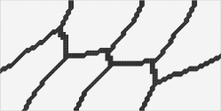
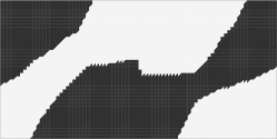
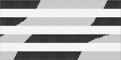
$N=8$ subdomains	$E=10^{5}$ (dark) or $10^{8}$ (light)	$E\mathrel{{+}{=}}10^{9}$ in white stripes
	‘no layers’	‘with layers’

Figure 1: Partition into subdomains, distribution of E without and with harder layers.

Let us recall that the size of the problem is $n=7224$. The computational domain $\Omega$ is partitioned into $N=8$ non-overlapping subdomains with Metis [24] (see Figure 1–left). The value of the coloring constant from Definition 1 is $\mathcal{N}=3$. There are $n_{\Gamma}=546$ degrees of freedom that belong to more than one subdomain. This is an important order of magnitude to compare the size of the coarse spaces to because it is always possible to eliminate all the degrees of freedom that are inside the subdomains and invert the $n_{\Gamma}\times n_{\Gamma}$ Schur complement. For a two-level method to be efficient, the cost of inverting the coarse space must be significantly less than the cost of inverting the Schur complement.

The first distribution of Young’s modulus $E$ is constant per subdomain: $E=10^{5}$ if $s$ is odd and $E=10^{8}$ if $s$ is even. The second distribution of Young’s modulus $E$ is obtained by adding some rigid layers to the first one: $E$ is augmented by $10^{9}$ if $y\in[1/7,2/7]\cup[3/7,4/7]\cup[5/7,6/7]$. These test cases are referred to as ‘no layers’ and ‘with layers’ and the coefficient distributions are plotted in Figure 1.

The first set of results is for Additive Schwarz. The first thing to check is that the condition numbers that are estimated satisfy the theoretical bounds. In Figure 2, the estimated condition numbers for the preconditioners $\mathbf{H}^{\text{AS}}_{ad}$ and $\mathbf{H}^{\text{AS}}_{hyb}$ introduced in Section 5.2.2 are represented for several values of $\tau_{\flat}$, with both $\mu$-scaling and $k$-scaling (i.e., $\mathbf{M}^{s}$ given by (19) or (20) in the generalized eigenvalue problems), and on both test cases. The theoretical bounds are also plotted. All the numerically obtained condition numbers are below the theoretical bound. The theoretical bound is less sharp when $\tau_{\flat}$ becomes larger: the numerically obtained conditioned bounds don’t degrade as much as the worst case scenario that is the theoretical bound. As expected, the hybrid preconditioned operator always has lower condition numbers than the corresponding additive preconditioned operator. Of course, this plot only tells one part of the story since it does not include any information about the cost of the methods. Table  1 gives a lot more information. Only the test case with layers is considered. In all four configurations (hybrid/additive and $\mu$-scaling/$k$-scaling), the choice $\tau_{\flat}=10$ seems to offer a good compromise between the condition number (or number of iterations) and the size of the coarse space. With the same value $\tau_{\flat}=10$, there is a big difference between the size of the coarse space with multiplicity scaling (241) and the size of the coarse space with $k$-scaling (68). With multiplicity scaling the table tells us that there is at least one subdomain that contributes 70 vectors to the coarse space. This is due to the fact that the $k$-scaling already contributes to handling the jumps in $E$ across the subdomains. To better illustrate this behaviour, Figure 3 shows the eigenvalues of the generalized eigenvalue problem solved to compute the coarse space. It becomes clear that the subdomains with $E=10^{8}$ will contribute many vectors for any desirable $\tau_{\flat}$. This may appear to be a failure of the GenEO method but it is highly unlikely that an automatic graph partitioner would produce such a configuration. A human partitioner might choose such a configuration but if that were the case, she would be aware of it and choose the scaling accordingly.

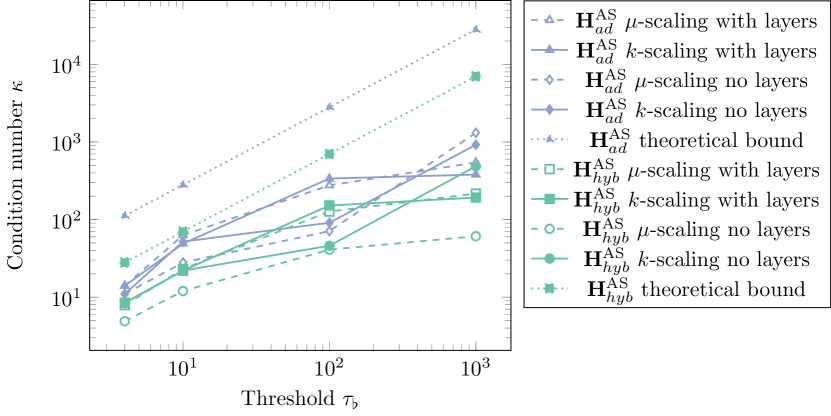
Figure 2: Condition numbers for Additive Schwarz preconditioners: additive and hybrid; $\mu$-scaling and $k$-scaling; with and without layers; $\tau\in[4;\,10;\,100;\,1000]$. All condition numbers are below the theoretical bound.

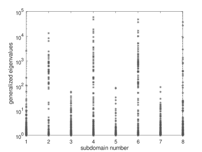
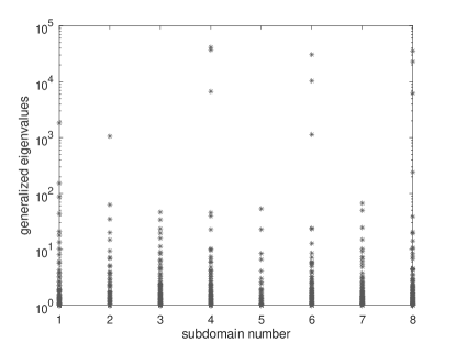
Figure 3: Solution of the generalized eigenvalue problem for computing $V^{0}_{\text{AS}}$ in the case with layers. Left: $\mu$-scaling, right: $k$-scaling.

For lack of space the results for Neumann-Neumann and Inexact Schwarz are presented in a lot less detail. The condition numbers for all methods are plotted with respect to the size of the coarse space for several values of $\tau_{\flat}$ and $\tau_{\sharp}$ (that are not reported here) in Figure 4 (test case without layers) and Figure 5 (test case with layers). In this plot, the best methods are the ones which have data points closest to the origin (small condition number with a small coarse space). It appears clearly that $k$-scaling gives better results. This was previously explained, but it is to be noted that with irregular subdomains, when the jumps in the coefficients become larger, the $k$-scaling can lead to very ill conditioned matrices $\mathbf{D}^{s}_{k}$ that can make the whole method less efficient again. This problem is well known and independent of GenEO. When there are no hard layers, the Neumann-Neumann method is the most impacted by the multiplicity scaling. This is to be expected because the matrices $\mathbf{D}^{s}_{k}$ appear in the definition of the one-level preconditioner and not only through the generalized eigenvalue problem that is solved to compute the coarse space. With $k$-scaling the methods from most to least efficient rank as follows: Neumann-Neumann, Additive Schwarz with hybrid preconditioner, Additive Schwarz with additive preconditioner, Inexact Schwarz. Again, this does not tell the whole story as the cost of one iteration depends on the choice of method. With inexact Schwarz, the local solves are cheapest. With additive Schwarz in the additive variant, the coarse solve can be done in parallel to the local solves. With Neumann-Neumann, the matrices that must be handled with most care numerically (the ones that are singular) are the local solvers whereas they only appear in the generalized eigenvalue problem for the other methods. All these arguments lead only to one conclusion: it is impossible from this data to tell which of the methods is most efficient. Numerical testing with measurements of the CPU time, memory requirements and overall stability of the algorithm is required. The answer would probably be problem dependant and is well beyond the scope of this article. Another question that has not been addressed yet is scalability. It is clearly guaranteed theoretically and illustrations can be found in the original articles [44, 45] with very similar coarse spaces.

As a final remark on Figure 4 and Figure 5, let us comment on the zig-zags in the Inexact Schwarz data in Figure 5. Since there are two parameters for the Inexact Schwarz coarse space, there are several choices of parameters that lead to coarse spaces that have the same size with possibly very different condition numbers. The local solvers being incomplete Cholesky factorizations of $\mathbf{R}^{s}\mathbf{A}{\mathbf{R}^{s}}^{\top}$ it is mostly only adding vectors to $V^{0}_{\flat}$ that makes the method more efficient while adding vectors to $V^{0}_{\sharp}$ makes the coarse space grow very fast and the condition number decrease very little.

Additive Schwarz with $\mu$-scaling ($\mathbf{M}^{s}_{\mu}$ from (19) in gevp) $\lambda_{\min}$ $\lambda_{\max}$ $\kappa$ It (final error) $\#V^{0}$ $\min\#V^{0}_{s}$ $\max\#V^{0}_{s}$ one-level $7.7\cdot 10^{-4}$ 3.0 3875 $>100$ ($6\cdot 10^{-3}$) 0 0 0 $\tau_{\flat}=10^{10}$ hyb 0.003 3.0 959 $>100$ ($1\cdot 10^{-5}$) 18 0 3 (only $\operatorname{Ker}(\mathbf{M}^{s})$) ad 0.002 3.3 1517 $>100$ ($3\cdot 10^{-4}$) 18 0 3 $\tau_{\flat}=1000$ hyb 0.014 3.0 216 $>100$ ($1\cdot 10^{-9}$) 72 1 24 ad 0.007 4.0 545 $>100$ ($1\cdot 10^{-6}$) 72 1 24 $\tau_{\flat}=100$ hyb 0.024 3.0 127 92 159 3 60 ad 0.014 4.0 276 $>100$ ($1\cdot 10^{-7}$) 159 3 60 $\tau_{\flat}=10$ hyb 0.13 3.0 23 42 241 10 70 ad 0.06 4.0 63 64 241 10 70 $\tau_{\flat}=4$ hyb 0.37 3.0 7.9 23 303 14 77 ad 0.28 4.0 14 31 303 14 77 Theory ($\tau_{\flat}$) hyb $1/\tau_{\flat}$ $\mathcal{N}=3$ $3\tau_{\flat}$ ad $1/(7\tau_{\flat})$ $\mathcal{N}+1=4$ $28\tau_{\flat}$ Additive Schwarz with $k$-scaling ($\mathbf{M}^{s}_{k}$ from (20) in gevp) $\lambda_{\min}$ $\lambda_{\max}$ $\kappa$ It (final error) $\#V^{0}$ $\min\#V^{0}_{s}$ $\max\#V^{0}_{s}$ one-level $7.7\cdot 10^{-4}$ 3.0 3875 $>100$ ($6\cdot 10^{-3}$) 0 0 0 $\tau_{\flat}=10^{10}$ hyb 0.0030 3.0 1003 $>100$ ($2\cdot 10^{-5}$) 18 0 3 (only $\operatorname{Ker}(\mathbf{M}^{s})$) ad 0.0025 3.2 1271 $>100$ ($2\cdot 10^{-4}$) 18 0 3 $\tau_{\flat}=1000$ hyb 0.016 3.0 192 98 29 1 6 ad 0.0087 3.3 380 $>100$ ($3\cdot 10^{-7}$) 29 1 6 $\tau_{\flat}=100$ hyb 0.02 3.0 152 93 31 1 7 ad 0.098 3.3 338 $>100$ ($2\cdot 10^{-7}$) 31 1 7 $\tau_{\flat}=10$ hyb 0.13 3.0 22 43 68 5 13 ad 0.069 3.37 49 63 68 5 13 $\tau_{\flat}=4$ hyb 0.35 3.0 8.5 26 118 8 20 ad 0.25 3.4 14 34 118 8 20 Theory ($\tau_{\flat}$) hyb $1/\tau_{\flat}$ $\mathcal{N}=3$ $3\tau_{\flat}$ ad $1/(7\tau_{\flat})$ $\mathcal{N}+1=4$ $28\tau_{\flat}$

Table 1: Test case with hard layers - All additive Schwarz methods - $\lambda_{\min}$ and $\lambda_{\max}$: extreme eigenvalues, $\kappa$: condition number, It: iteration count (with relative error at iteration 100 in parenthesis if the method has not converged), $\#V^{0}$ : dimension of the coarse space, $\min\#V^{0}_{s}$: number of coarse vectors contributed by the subdomain that contributes the fewest vectors, $\max\#V^{0}_{s}$: number of coarse vectors contributed by the subdomain that contributes the most eigenvectors, gevp: generalized eigenvalue problem. The one-level method does not satisfy any theoretical bound for $\lambda_{\min}$.

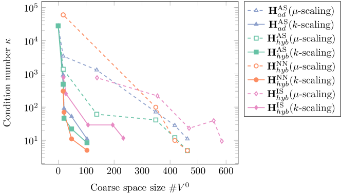
Figure 4: Efficiency of the methods for the test case without layers

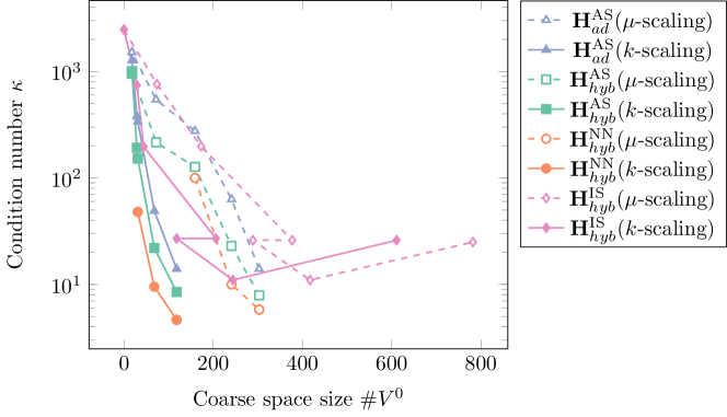
Figure 5: Efficiency of the methods for the test case with layers

6 Conclusion

GenEO coarse spaces have been introduced for all domain decomposition methods in the abstract Schwarz framework that satisfy some clearly stated assumptions. By solving one or two generalized eigenvalue problems in each subdomain, it is possible to construct a method for which the eigenvalues of the preconditioned operator are bounded as desired. Proofs of these bounds were given for the projected preconditioned operators, the hybrid operators and, when possible, the additive operators. Finally, the method was applied to a linear elasticity problem discretized by $\mathbb{P}_{1}$ finite elements. The results in the last section could very easily be applied to any elliptic PDE, just by changing the definitions of $\mathbf{A}$ and the matrices $\mathbf{A}_{|\Omega^{s}}^{s}$. The most restrictive assumption in the construction of the coarse space is Assumption 5. If a two-level method with guaranteed convergence existed without that assumption it would be even easier to implement in a black box fashion and this will be the topic of future work.

References

- [1] E. Agullo, L. Giraud, and L. Poirel. Robust preconditioners via generalized eigenproblems for hybrid sparse linear solvers. SIAM Journal on Matrix Analysis and Applications, 40(2):417–439, 2019.
- [2] A. Ben-Israel. The Moore of the Moore-Penrose inverse. The Electronic Journal of Linear Algebra, 9, 2002.
- [3] M. Brezina, C. Heberton, J. Mandel, and P. Vaněk. An iterative method with convergence rate chosen a priori. Technical Report 140, University of Colorado Denver, April 1999.
- [4] J. G. Calvo and O. B. Widlund. An adaptive choice of primal constraints for BDDC domain decomposition algorithms. Electron. Trans. Numer. Anal, 45:524–544, 2016.
- [5] T. F. Chan and H. A. Van Der Vorst. Approximate and incomplete factorizations. In Parallel numerical algorithms, pages 167–202. Springer, 1997.
- [6] T. Chartier, R. D. Falgout, V. E. Henson, J. Jones, T. Manteuffel, S. McCormick, J. Ruge, and P. S. Vassilevski. Spectral AMGe (AMGe). SIAM J. Sci. Comput., 25(1):1–26, 2003.
- [7] L. B. Da Veiga, L. F. Pavarino, S. Scacchi, O. B. Widlund, and S. Zampini. Adaptive selection of primal constraints for isogeometric BDDC deluxe preconditioners. SIAM Journal on Scientific Computing, 39(1):A281–A302, 2017.
- [8] V. Dolean, P. Jolivet, and F. Nataf. An introduction to domain decomposition methods. Society for Industrial and Applied Mathematics (SIAM), Philadelphia, PA, 2015. Algorithms, theory, and parallel implementation.
- [9] V. Dolean, F. Nataf, R. Scheichl, and N. Spillane. Analysis of a two-level Schwarz method with coarse spaces based on local Dirichlet-to-Neumann maps. Comput. Methods Appl. Math., 12(4):391–414, 2012.
- [10] Z. Dostál. Conjugate gradient method with preconditioning by projector. International Journal of Computer Mathematics, 23(3-4):315–323, 1988.
- [11] M. Dryja and O. B. Widlund. Schwarz methods of Neumann-Neumann type for three-dimensional elliptic finite element problems. Communications on pure and applied mathematics, 48(2):121–155, 1995.
- [12] J. W. Eaton, D. Bateman, S. Hauberg, and R. Wehbring. GNU Octave version 5.2.0 manual: a high-level interactive language for numerical computations, 2020.
- [13] Y. Efendiev, J. Galvis, R. Lazarov, and J. Willems. Robust domain decomposition preconditioners for abstract symmetric positive definite bilinear forms. ESAIM Math. Model. Numer. Anal., 46(5):1175–1199, 2012.
- [14] C. Farhat and F.-X. Roux. A method of finite element tearing and interconnecting and its parallel solution algorithm. Internat. J. Numer. Methods Engrg., 32:1205–1227, 1991.
- [15] J. Galvis and Y. Efendiev. Domain decomposition preconditioners for multiscale flows in high-contrast media. Multiscale Model. Simul., 8(4):1461–1483, 2010.
- [16] J. Galvis and Y. Efendiev. Domain decomposition preconditioners for multiscale flows in high contrast media: reduced dimension coarse spaces. Multiscale Model. Simul., 8(5):1621–1644, 2010.
- [17] M. J. Gander and A. Loneland. Shem: An optimal coarse space for ras and its multiscale approximation. In Domain decomposition methods in science and engineering XXIII, pages 313–321. Springer, 2017.
- [18] G. H. Golub and C. F. van Loan. Matrix Computations. JHU Press, fourth edition, 2013.
- [19] I. G. Graham, P. Lechner, and R. Scheichl. Domain decomposition for multiscale PDEs. Numerische Mathematik, 106(4):589–626, 2007.
- [20] R. Haferssas, P. Jolivet, and F. Nataf. An additive Schwarz method type theory for Lions’s algorithm and a symmetrized optimized restricted additive Schwarz method. SIAM Journal on Scientific Computing, 39(4):A1345–A1365, 2017.
- [21] F. Hecht. New development in FreeFem++. J. Numer. Math., 20(3-4):251–265, 2012.
- [22] A. Heinlein, A. Klawonn, J. Knepper, and O. Rheinbach. Adaptive gdsw coarse spaces for overlapping schwarz methods in three dimensions. SIAM Journal on Scientific Computing, 41(5):A3045–A3072, 2019.
- [23] V. Hernandez, J. E. Roman, and V. Vidal. SLEPc: A scalable and flexible toolkit for the solution of eigenvalue problems. ACM Trans. Math. Software, 31(3):351–362, 2005.
- [24] G. Karypis and V. Kumar. A fast and high quality multilevel scheme for partitioning irregular graphs. SIAM J. Sci. Comput., 20(1):359–392 (electronic), 1998.
- [25] H. H. Kim, E. Chung, and J. Wang. BDDC and FETI-DP preconditioners with adaptive coarse spaces for three-dimensional elliptic problems with oscillatory and high contrast coefficients. Journal of Computational Physics, 349:191–214, 2017.
- [26] A. Klawonn, M. Kuhn, and O. Rheinbach. Adaptive coarse spaces for FETI-DP in three dimensions. SIAM Journal on Scientific Computing, 38(5):A2880–A2911, 2016.
- [27] A. Klawonn, M. Lanser, and O. Rheinbach. Toward extremely scalable nonlinear domain decomposition methods for elliptic partial differential equations. SIAM Journal on Scientific Computing, 37(6):C667–C696, 2015.
- [28] A. Klawonn, P. Radtke, and O. Rheinbach. A comparison of adaptive coarse spaces for iterative substructuring in two dimensions. Electron. Trans. Numer. Anal, 45:75–106, 2016.
- [29] A. Klawonn and O. Rheinbach. Deflation, projector preconditioning, and balancing in iterative substructuring methods: connections and new results. SIAM J. Sci. Comput., 34(1):A459–A484, 2012.
- [30] A. Klawonn and O. B. Widlund. FETI and Neumann-Neumann iterative substructuring methods: connections and new results. Comm. Pure Appl. Math., 54(1):57–90, 2001.
- [31] J. Mandel and B. Sousedík. Adaptive selection of face coarse degrees of freedom in the BDDC and the FETI-DP iterative substructuring methods. Comput. Methods Appl. Mech. Engrg., 196(8):1389–1399, 2007.
- [32] P. Marchand, X. Claeys, P. Jolivet, F. Nataf, and P.-H. Tournier. Two-level preconditioning for h-version boundary element approximation of hypersingular operator with GenEO. Numerische Mathematik, 146(3):597–628, 2020.
- [33] G. Meurant and P. Tichỳ. Approximating the extreme Ritz values and upper bounds for the A-norm of the error in CG. Numerical Algorithms, 82(3):937–968, 2019.
- [34] F. Nataf, H. Xiang, and V. Dolean. A two level domain decomposition preconditioner based on local Dirichlet-to-Neumann maps. C. R. Math. Acad. Sci. Paris, 348(21-22):1163–1167, 2010.
- [35] F. Nataf, H. Xiang, V. Dolean, and N. Spillane. A coarse space construction based on local Dirichlet-to-Neumann maps. SIAM J. Sci. Comput., 33(4):1623–1642, 2011.
- [36] C. Pechstein and C. R. Dohrmann. A unified framework for adaptive BDDC. Electron. Trans. Numer. Anal, 46(273-336):3, 2017.
- [37] C. Pechstein and R. Scheichl. Analysis of FETI methods for multiscale PDEs. Numer. Math., 111(2):293–333, 2008.
- [38] C. Pechstein and R. Scheichl. Scaling up through domain decomposition. Appl. Anal., 88(10-11):1589–1608, 2009.
- [39] C. Pechstein and R. Scheichl. Analysis of FETI methods for multiscale PDEs. Part II: interface variation. Numer. Math., 118(3):485–529, 2011.
- [40] C. Pechstein and R. Scheichl. Weighted Poincaré inequalities. IMA J. Numer. Anal., 33(2):652–686, 2013.
- [41] M. Sarkis. Partition of unity coarse spaces: enhanced versions, discontinuous coefficients and applications to elasticity. Domain decomposition methods in science and engineering, pages 149–158, 2003.
- [42] B. Sousedík, J. Šístek, and J. Mandel. Adaptive-Multilevel BDDC and its parallel implementation. Computing, 95(12):1087–1119, 2013.
- [43] N. Spillane, V. Dolean, P. Hauret, F. Nataf, C. Pechstein, and R. Scheichl. A robust two-level domain decomposition preconditioner for systems of PDEs. C. R. Math. Acad. Sci. Paris, 349(23-24):1255–1259, 2011.
- [44] N. Spillane, V. Dolean, P. Hauret, F. Nataf, C. Pechstein, and R. Scheichl. Abstract robust coarse spaces for systems of PDEs via generalized eigenproblems in the overlaps. Numer. Math., 126(4):741–770, 2014.
- [45] N. Spillane and D. J. Rixen. Automatic spectral coarse spaces for robust FETI and BDD algorithms. Int. J. Numer. Meth. Engng., 95(11):953–990, 2013.
- [46] J. M. Tang, R. Nabben, C. Vuik, and Y. A. Erlangga. Comparison of two-level preconditioners derived from deflation, domain decomposition and multigrid methods. J. Sci. Comput., 39(3):340–370, 2009.
- [47] A. Toselli and O. Widlund. Domain decomposition methods—algorithms and theory, volume 34 of Springer Series in Computational Mathematics. Springer-Verlag, Berlin, 2005.
- [48] Y. Yu, M. Dryja, and M. Sarkis. From Additive Average Schwarz Methods to Non-overlapping Spectral Additive Schwarz Methods. arXiv preprint arXiv:2012.13610, 2020.
- [49] S. Zampini. PCBDDC: a class of robust dual-primal methods in PETSc. SIAM Journal on Scientific Computing, 38(5):S282–S306, 2016.