Efficient Set-Based Approaches for the Reliable Computation of Robot Capabilities

Abstract

To reliably model real robot characteristics, interval linear systems of equations allow to describe families of problems that consider sets of values. This allows to easily account for typical complexities such as sets of joint states and design parameter uncertainties. Inner approximations of the solutions to the interval linear systems can be used to describe the common capabilities of a robotic manipulator corresponding to the considered sets of values. In this work, several classes of problems are considered. For each class, reliable and efficient polytope, n-cube, and n-ball inner approximations are presented.

The interval approaches usually proposed are inefficient because they are too computationally heavy for certain applications, such as control. We propose efficient new inner approximation theorems for the considered classes of problems. This allows for usage with real-time applications as well as rapid analysis of potential designs. Several applications are presented for a redundant planar manipulator including locally evaluating the manipulator’s velocity, acceleration, and static force capabilities, and evaluating its future acceleration capabilities over a given time horizon.

I Introduction

The capability of a robot to autonomously adapt to an open dynamic environment is one of the ultimate challenges of robotics.

One of the keys to solve this challenge lies in the ability to dynamically control the motion of the robot as a function of the prediction of the environment dynamics in order to both optimally achieve the goals assigned to the robot while ensuring safety at all times. In other words, planning and control can no longer be considered as two separated problems solved sequentially. Indeed, this kind of approach works well only for simple robots evolving in static environments and solving basic tasks, where a large amount of time can be spent planning the motion offline and where the control problem consists of tracking, with almost no adaptation, the planned trajectory.

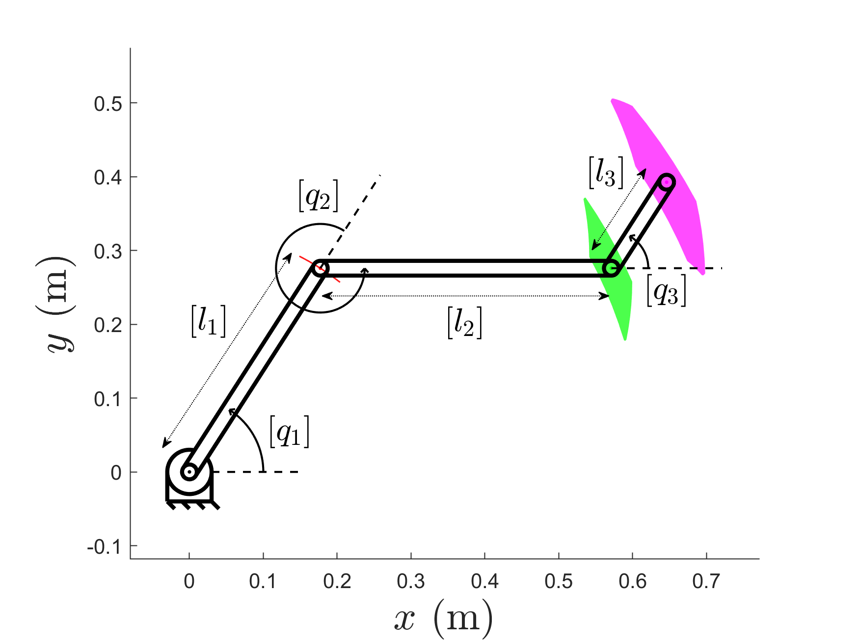
Figure 1: The sets of positions associated with the distal ends of the links for the set of configurations $[\operatorname{{\bf q}}]=(1.0,-1.0,1.0)\pm 0.1$ rads for a family of three-link planar manipulators with parameter values $[\operatorname{{\bf l}}]=(0.3280,0.3940,0.1385)\pm 0.001$ m. The red, green, and purple regions are the corresponding positions of the distal ends of the first, second, and third links respectively.

Beyond the perception abilities needed to estimate the state of the robot with respect to its environment, dynamic contexts require to adapt the planned motion at all time. For this adaptation to be optimal, it should not be purely reactive but rather adapt the overall plan online, i.e., at each control instant. While the concept of online re-planning is appealing, it raises the question of the real-time tractability of the corresponding optimization problems. As explained in [1], in the very challenging case of humanoid robots, accounting for limited computation power, one can choose to make use of rather precise models of the robot’s dynamics and constraints but the price to pay for this modeling complexity is the limited time horizon over which planning can be considered, leading to feasible but potentially sub-optimal robot behaviours. On the other hand, one can decide to plan over longer time horizons, for example using optimal control approaches or their receding horizon version such as Model Predictive Control (MPC). In return, one has to make use of simpler models to maintain a low computation complexity for online re-planning to be possible. This is typically the approach taken when planning for locomotion in humanoid robotics: given a target position in Cartesian space, one first computes a desired trajectory for an abstracted version of the system, typically its centre of mass (CoM) and the associated centroidal dynamics. Then one defines a sequence of contacts and associated stances that are both compatible with the desired CoM trajectory and physically viable. Finally, using a more complete model of the system, a whole-body control approach is used to compute the actuation inputs allowing to follow the trajectory joining two consecutive stances and associated contact states [2]. The latter approach seems more appropriate in terms of the optimality of the obtained behaviours but also in terms of the involved computations. Indeed, while recent works on Differential Dynamic Programming [3] tackle the full model problem over the full horizon, these approaches remain computationally too complex for online re-planning on real robots and it actually does not seem quite necessary to plan precisely joint level actuation over a long time horizon.

If approaches resorting to simplified models seem more appropriate, an abstract model of the system still requires to be connected to a more physically realistic one for control purposes. While this connection can be made through task level abstractions, it is also necessary to account for the low level limits of the robot at the planning level in order to produce plans that can be achieved by the robots given its intrinsic (e.g., joint limits) and extrinsic (e.g., collision avoidance) constraints. Often in robotics, accounting for the joint level limitations at the more abstract level of task description is a matter of manual tuning and heuristics as solving this problem formally and in a computationally efficient manner is complex. Going beyond simple heuristics and assuming constant task level acceleration capabilities (e.g. the ones provided by robot manufacturers), some work have been performed in the past to account for acceleration limits at the joint level while accounting for the potential incompatibilities between these acceleration limits and position ones [4, 5, 6]. While of interest, these works fail short at accounting in a formal way for the true limits of robots which are best expressed at the joint level in terms of joint position, velocity, torque and torque derivative. Indeed, one of the main difficulties with joint level acceleration limits is that they are state dependant. This is all the more true when considering the expression of these limits in Cartesian space as the mappings from joint space to task space, being them at the static or dynamic level, are both state dependant and non-linear. In order to tackle this complexity, there is a need for new methodologies that are able to efficiently, accurately and with a limited computation cost predict the robot’s capabilities in static but more importantly in dynamic scenarios. Furthermore, these methodologies should be able to handle imprecise/variable systems by accounting for system complexities such as sets of joint states and design parameter uncertainties to produce reliable results. Accounting for these uncertainties is of high importance when dealing with floating base systems such as humanoids or mobile robots in general [7]. Thus, modeling errors and state changes over a given time horizon should be properly accounted for when computing capabilities.

With this overall motivation in mind, this work presents several classes of problems that can be used to reliably and efficiently compute polytope, n-cube, and n-ball inner approximations of the capabilities of robotic systems, being them imprecise or uncertain.

The descriptions of the capabilities of many robotics systems can be formulated in terms of linear systems of equations

$$\operatorname{{\bf A}}\operatorname{{\bf x}}=\operatorname{{\bf b}}$$ (1)

with $\operatorname{{\bf A}}\in\mathbb{R}^{m\times n}$, $\operatorname{{\bf x}}\in\mathbb{R}^{n}$, and $\operatorname{{\bf b}}\in\mathbb{R}^{m}$. These linear equations may be used to describe specific capabilities of a robotic manipulator for a unique configuration ${\operatorname{{\bf q}}}$ or state $\{{\operatorname{{\bf q}}},{\bf\dot{q}}\}$. In offline applications, the evaluation of robot capabilities allows to analyze the performance of a given design and may be used during the dimensional synthesis stage of robotic design. In online applications, the current and/or future robot capabilities can be computed and may be used to autonomously re-plan and control the motion of the robot.

For example, for serial manipulators at the velocity kinematic level one may consider the:

• velocity kinematics model:

  $${\operatorname{{\bf J}}}({\operatorname{{\bf q}}})\dot{\operatorname{{\bf q}}}=\dot{\operatorname{{\bf x}}}$$ (2)

  where ${\operatorname{{\bf J}}}({\operatorname{{\bf q}}})$ is the Jacobian matrix, and $\dot{\operatorname{{\bf q}}}$ and $\dot{\operatorname{{\bf x}}}$ are the joint and operational velocities respectively.

• kinetostatic model

  $${\operatorname{{\bf J}}}({\operatorname{{\bf q}}})^{T}{\bf f}=\boldsymbol{\tau}$$ (3)

  where ${\bf f}$ is the operational wrench and $\boldsymbol{\tau}$ is the joint torque/force vector.

At the dynamic level, one may also characterize the capabilities of a robot through the:

• forward acceleration model:

  $$\dot{\operatorname{{\bf J}}}({\operatorname{{\bf q}}},\dot{\operatorname{{\bf q}}})\dot{\operatorname{{\bf q}}}+{\operatorname{{\bf J}}}({\operatorname{{\bf q}}})\ddot{\operatorname{{\bf q}}}=\ddot{\operatorname{{\bf x}}}$$ (4)

  where $\dot{\operatorname{{\bf J}}}({\operatorname{{\bf q}}},\dot{\operatorname{{\bf q}}})$ is the time derivative of the Jacobian matrix, and $\ddot{\operatorname{{\bf q}}}$ and $\ddot{\operatorname{{\bf x}}}$ are the joint and operational accelerations respectively.

• configuration-space dynamic model:

  $${\bf M}({\operatorname{{\bf q}}})\ddot{\operatorname{{\bf q}}}=\boldsymbol{\tau}-{\operatorname{{\bf c}}}({\operatorname{{\bf q}}},\dot{\operatorname{{\bf q}}})-{\operatorname{{\bf g}}}({\operatorname{{\bf q}}})$$ (5)

  where ${\bf M({\operatorname{{\bf q}}})}$ is the mass matrix, ${\operatorname{{\bf c}}}({\operatorname{{\bf q}}},\dot{\operatorname{{\bf q}}})$ is the centrifugal and Coriolis vector and ${\operatorname{{\bf g}}}({\operatorname{{\bf q}}})$ is the gravity vector.

• operational-space dynamic problem:

  $$\boldsymbol{\Lambda}({\operatorname{{\bf q}}})\ddot{\operatorname{{\bf x}}}={\bf f}-\boldsymbol{\mu}({\operatorname{{\bf q}}},\dot{\operatorname{{\bf q}}})-{\bf p}({\operatorname{{\bf q}}})$$ (6)

  where $\boldsymbol{\Lambda}({\operatorname{{\bf q}}})$ is the Cartesian mass matrix, $\boldsymbol{\mu}({\operatorname{{\bf q}}},\dot{\operatorname{{\bf q}}})$ is the centrifugal and Coriolis vector in Cartesian space and ${\bf p}({\operatorname{{\bf q}}})$ is the gravity vector in Cartesian space.

Due to the many sources of uncertainties that exist (e.g., noisy sensor data, modeling errors), to reliably predict the capabilities of the robot it can be desirable to consider sets of robot models and states. Using interval analysis (see [8, 9, 10]), it is possible to extend these problems in order to describe a family of problems that consider sets of values (e.g., sets of design parameters, sets of configurations $[{\operatorname{{\bf q}}}]$, sets of joint velocities $[\dot{\operatorname{{\bf q}}}]$, etc.). Figure 1 depicts a family of three-link planar manipulators with sets of link lengths, $[l_{1}]$, $[l_{2}]$, and $[l_{3}]$, and sets of configurations, $[q_{1}]$, $[q_{2}]$, and $[q_{3}]$, and shows the corresponding sets of positions associated with the distal ends of the links for the given configurations (53) and design parameters (51). The set of configurations may be used to model dimensional uncertainties in the system, and may also be used to model the temporal evolution of the system. The set-based approaches presented in this work can be used to reliably predict the robot’s various capabilities for these type of problems, where the reliable and efficient evaluation of imprecise/variable systems and their current or future capabilities over a given prediction period provides many avenues for improving the performance and safety of robotic manipulators. Classes of problems may be described in terms of quantifiers which allow to describe reliable inner approximations of the capabilities of a robot over sets of values. Alternatively, reliable outer approximations may also be computed [11, 12, 13, 14], although these types of problems are not considered in this work. Considering velocity kinematics related models, when a set of configurations $[{\operatorname{{\bf q}}}]$ are considered the Jacobian matrix ${\operatorname{{\bf J}}}$ becomes an interval matrix $[{\operatorname{{\bf J}}}]$. Generally, the evaluation of $[{\operatorname{{\bf J}}}]$ is overestimated due to the interval wrapping effect [15] and dependency problem [16] and there exists some matrices ${\operatorname{{\bf J}}}_{o}\in[{\operatorname{{\bf J}}}]$ such that ${\operatorname{{\bf J}}}_{o}\not\in\{{\operatorname{{\bf J}}}({\operatorname{{\bf q}}})~{}|~{}{\operatorname{{\bf q}}}\in[{\operatorname{{\bf q}}}]\}$. Nevertheless, each ${\operatorname{{\bf J}}}\in[{\operatorname{{\bf J}}}]$ has associated capabilities and the intersection of these capabilities describes the common capabilities for all configurations ${\operatorname{{\bf q}}}\in[{\operatorname{{\bf q}}}]$. This extends to the dynamic models similarly.

The interval analysis framework has proven to be a useful tool for the analysis and synthesis of robotic mechanisms as it guarantees certified numerical solutions to problems [17]. When combined with classical branch-and-bound approaches, entire parameter spaces can be thoroughly and reliably explored allowing the worst-case conditions throughout the parameter space to be properly understood. Such an approach has been widely used for workspace analysis, e.g., considering flexure-jointed mechanisms [18], evaluating wrench capabilities [19, 20] and positioning errors [21], and computing collision-free poses [22] and singularity-free poses [23, 24].

By considering the intersections of manipulator capabilities for all values in the sets, this allows to compute common capabilities of the robotic manipulator corresponding to the considered sets of values. To reliably describe the capabilities of a robotic manipulator corresponding to a set of values, inner approximations of the intersections of manipulator capabilities must be computed. For a given interval linear system of equations, several classes of problems may be considered. The main contribution of this work is the development of efficient polytope, n-cube, and n-ball inner approximations which are applicable to each class of problem considered. Furthermore, these inner approximations are applied to several relevant robotics problems to demonstrate their capability to easily handle typical complexities such as sets of joint states and design parameter uncertainties.

The remainder of this paper is as follows. First, in Section II the relevant interval notations are introduced. Next, in Section III the classes of interval linear system of equation problems considered in this work are described. In Section IV the polytope, n-cube, and n-ball inner approximations for each class of problem are presented. Several applications are presented in Section V for a redundant planar manipulator to locally evaluate the manipulator’s velocity, static force, and acceleration capabilities, and also its future acceleration capabilities over a given time horizon.

II Notation

The interval extension of a variable $x$ is given by

$$[x]=\{x~{}|~{}\underline{{x}}\leq x\leq\overline{{x}}\}$$ (7)

where $\underline{{x}}$ is the lower bound (infimum) $\underline{{x}}={\operatorname{inf}{\left({x}\right)}}$ and $\overline{{x}}$ is the upper bound (supremum) $\overline{{x}}={\operatorname{sup}{\left({x}\right)}}$ of the interval.

A few terms useful in this work are:

1. The midpoint of an interval is the real value given by

   $${\operatorname{mid}\left\lparen[x]\right\rparen}=\frac{1}{2}(\underline{{x}}+\overline{{x}})$$ (8)

2. The radius of an interval is the real value given by

   $${\operatorname{\Delta}{[}}x]=\frac{1}{2}(\overline{{x}}-\underline{{x}})$$ (9)

3. The mignitude of an interval is the real value given by

   $${\operatorname{mig}{\left({[x]}\right)}}=\min(\{{|{x}|}~{}|~{}x\in[x]\})$$ (10)

4. The magnitude of an interval is the real value given by

   $${\operatorname{mag}\left\lparen[x]\right\rparen}=\max(\{{|{x}|}~{}|~{}x\in[x]\})$$ (11)

5. The absolute value of an interval is the interval given by

   $${|{[x]}|}=[{\operatorname{mig}{\left({[x]}\right)}},{\operatorname{mag}\left\lparen[x]\right\rparen}]$$ (12)

Let a vector and matrix be given by $\operatorname{{\bf x}}$ and $\operatorname{{\bf A}}$ respectively. The interval extensions of the vector and matrix are then given by $[\operatorname{{\bf x}}]$ and $[\operatorname{{\bf A}}]$ and the previously described terms may be applied to each element in the vector or matrix. Classes of problems may be described with the $\forall$ (for all) and $\exists$ (there exists) quantifiers which allow to describe reliable inner approximations to the interval linear system of equations over the considered sets of values.

III Classes of Problems

Several classes of problems are considered in this work which are presented in a general form $\operatorname{{\bf A}}\operatorname{{\bf x}}=\operatorname{{\bf b}}$. These problems and their corresponding sub-problems are as follows.

III-A Problems $\operatorname{\Omega_{\forall\exists}\left([\operatorname{{\bf A}}],[\operatorname{{\bf x}}]\right)}$ and $\operatorname{\Omega_{\forall\exists}\left(\operatorname{{\bf A}},[\operatorname{{\bf x}}]\right)}$

The first class of problems considered are of the form

$$\operatorname{\Omega_{\forall\exists}\left([\operatorname{{\bf A}}],[\operatorname{{\bf x}}]\right)}=\{\operatorname{{\bf b}}~{}|~{}(\forall\operatorname{{\bf A}}\in[\operatorname{{\bf A}}])(\exists\operatorname{{\bf x}}\in[\operatorname{{\bf x}}])(\operatorname{{\bf A}}\operatorname{{\bf x}}=\operatorname{{\bf b}})\}$$ (13)

which applies a set of linear transformations $[\operatorname{{\bf A}}]$ to a set of vectors $[\operatorname{{\bf x}}]$. The sub-problem

$$\operatorname{\Omega_{\forall\exists}\left(\operatorname{{\bf A}},[\operatorname{{\bf x}}]\right)}=\{\operatorname{{\bf b}}~{}|~{}(\exists\operatorname{{\bf x}}\in[\operatorname{{\bf x}}])(\operatorname{{\bf A}}\operatorname{{\bf x}}=\operatorname{{\bf b}})\}$$ (14)

is geometrically a convex polytope [25, 26, 27]. Therefore, (13) is equivalent to the intersection of all sub-problems $\operatorname{{\bf A}}\in[\operatorname{{\bf A}}]$. That is,

$$\operatorname{\Omega_{\forall\exists}\left([\operatorname{{\bf A}}],[\operatorname{{\bf x}}]\right)}=\bigcap_{\operatorname{{\bf A}}\in[\operatorname{{\bf A}}]}\operatorname{\Omega_{\forall\exists}\left(\operatorname{{\bf A}},[\operatorname{{\bf x}}]\right)}$$ (15)

III-B Problems $\operatorname{\Sigma_{\forall\exists}\left([\operatorname{{\bf A}}],[\operatorname{{\bf b}}]\right)}$ and $\operatorname{\Sigma_{\forall\exists}\left(\operatorname{{\bf A}},[\operatorname{{\bf b}}]\right)}$

The second class of problems considered are of the form

$$\operatorname{\Sigma_{\forall\exists}\left([\operatorname{{\bf A}}],[\operatorname{{\bf b}}]\right)}=\{\operatorname{{\bf x}}~{}|~{}(\forall\operatorname{{\bf A}}\in[\operatorname{{\bf A}}])(\exists~{}\operatorname{{\bf b}}\in[\operatorname{{\bf b}}])(\operatorname{{\bf A}}\operatorname{{\bf x}}=\operatorname{{\bf b}})\}$$ (16)

which is precisely the tolerance solution set of the interval linear system as described in [28]. Considering the sub-problem

$$\operatorname{\Sigma_{\forall\exists}\left(\operatorname{{\bf A}},[\operatorname{{\bf b}}]\right)}=\{\operatorname{{\bf x}}~{}|~{}(\exists~{}\operatorname{{\bf b}}\in[\operatorname{{\bf b}}])(\operatorname{{\bf A}}\operatorname{{\bf x}}=\operatorname{{\bf b}})\}$$ (17)

which is also geometrically a convex polytope, it is clear that

$$\operatorname{\Sigma_{\forall\exists}\left([\operatorname{{\bf A}}],[\operatorname{{\bf b}}]\right)}=\bigcap_{\operatorname{{\bf A}}\in[\operatorname{{\bf A}}]}\operatorname{\Sigma_{\forall\exists}\left(\operatorname{{\bf A}},[\operatorname{{\bf b}}]\right)}$$ (18)

III-C Robotics Use Cases

The use cases of each class of problem applied to the relevant robotics problems (2) – (6) are outlined in Tables I and II. The classes $\operatorname{\Omega_{\forall\exists}\left(\operatorname{{\bf A}},[\operatorname{{\bf x}}]\right)}$ and $\operatorname{\Sigma_{\forall\exists}\left(\operatorname{{\bf A}},[\operatorname{{\bf b}}]\right)}$ consider a unique configuration $\operatorname{{\bf q}}$ or state $\{\operatorname{{\bf q}},\dot{\operatorname{{\bf q}}}\}$ whereas the classes $\operatorname{\Omega_{\forall\exists}\left([\operatorname{{\bf A}}],[\operatorname{{\bf x}}]\right)}$ and $\operatorname{\Sigma_{\forall\exists}\left([\operatorname{{\bf A}}],[\operatorname{{\bf b}}]\right)}$ can consider a set of configuration $[\operatorname{{\bf q}}]$ or states $\{[\operatorname{{\bf q}}],[\dot{\operatorname{{\bf q}}}]\}$.

TABLE I: Inner approximation use cases for $\operatorname{\Omega_{\forall\exists}\left(\operatorname{{\bf A}},[\operatorname{{\bf x}}]\right)}$ and $\operatorname{\Omega_{\forall\exists}\left([\operatorname{{\bf A}}],[\operatorname{{\bf x}}]\right)}$

Problems	Unknown	Description of $\operatorname{\Omega_{\forall\exists}\left(\operatorname{{\bf A}},[\operatorname{{\bf x}}]\right)}$	Description of $\operatorname{\Omega_{\forall\exists}\left([\operatorname{{\bf A}}],[\operatorname{{\bf x}}]\right)}$
${\operatorname{{\bf J}}}({\operatorname{{\bf q}}})\dot{\operatorname{{\bf q}}}=\dot{\operatorname{{\bf x}}}$	$\dot{\operatorname{{\bf x}}}$	$\{\dot{\operatorname{{\bf x}}}~{}|~{}(\exists\dot{\operatorname{{\bf q}}}\in[\dot{\operatorname{{\bf q}}}])({\operatorname{{\bf J}}}({\operatorname{{\bf q}}})\dot{\operatorname{{\bf q}}}=\dot{\operatorname{{\bf x}}})\}$	$\{\dot{\operatorname{{\bf x}}}~{}|~{}(\forall{\operatorname{{\bf J}}}({\operatorname{{\bf q}}})\in{\operatorname{{\bf J}}}([{\operatorname{{\bf q}}}]))(\exists\dot{\operatorname{{\bf q}}}\in[\dot{\operatorname{{\bf q}}}])({\operatorname{{\bf J}}}({\operatorname{{\bf q}}})\dot{\operatorname{{\bf q}}}=\dot{\operatorname{{\bf x}}})\}$
${\operatorname{{\bf J}}}({\operatorname{{\bf q}}})^{T}{\bf f}=\boldsymbol{\tau}$	$\boldsymbol{\tau}$	$\{\boldsymbol{\tau}~{}|~{}(\exists{\bf f}\in[{\bf f}])({\operatorname{{\bf J}}}({\operatorname{{\bf q}}})^{T}{\bf f}=\boldsymbol{\tau})\}$	$\{\boldsymbol{\tau}~{}|~{}(\forall{\operatorname{{\bf J}}}({\operatorname{{\bf q}}})\in{\operatorname{{\bf J}}}([{\operatorname{{\bf q}}}]))(\exists{\bf f}\in[{\bf f}])({\operatorname{{\bf J}}}({\operatorname{{\bf q}}})^{T}{\bf f}=\boldsymbol{\tau})\}$
$\dot{\operatorname{{\bf J}}}({\operatorname{{\bf q}}},\dot{\operatorname{{\bf q}}})\dot{\operatorname{{\bf q}}}+{\operatorname{{\bf J}}}({\operatorname{{\bf q}}})\ddot{\operatorname{{\bf q}}}=\ddot{\operatorname{{\bf x}}}$	$\ddot{\operatorname{{\bf x}}}$	$\{\ddot{\operatorname{{\bf x}}}~{}|~{}(\exists\dot{\operatorname{{\bf q}}}\in[\dot{\operatorname{{\bf q}}}])(\dot{\operatorname{{\bf J}}}({\operatorname{{\bf q}}},\dot{\operatorname{{\bf q}}})\dot{\operatorname{{\bf q}}}=\ddot{\operatorname{{\bf x}}})\}$	$\{\ddot{\operatorname{{\bf x}}}~{}|~{}(\forall\dot{\operatorname{{\bf J}}}({\operatorname{{\bf q}}},\dot{\operatorname{{\bf q}}})\in\dot{\operatorname{{\bf J}}}([{\operatorname{{\bf q}}}],[\dot{\operatorname{{\bf q}}}]))(\exists\dot{\operatorname{{\bf q}}}\in[\dot{\operatorname{{\bf q}}}])(\dot{\operatorname{{\bf J}}}({\operatorname{{\bf q}}},\dot{\operatorname{{\bf q}}})\dot{\operatorname{{\bf q}}}=\ddot{\operatorname{{\bf x}}})\}$
		$+\{\ddot{\operatorname{{\bf x}}}~{}|~{}(\exists\ddot{\operatorname{{\bf q}}}\in[\ddot{\operatorname{{\bf q}}}])({\operatorname{{\bf J}}}({\operatorname{{\bf q}}})\ddot{\operatorname{{\bf q}}}=\ddot{\operatorname{{\bf x}}})\}$	$+\{\ddot{\operatorname{{\bf x}}}~{}|~{}(\forall{\operatorname{{\bf J}}}({\operatorname{{\bf q}}})\in{\operatorname{{\bf J}}}([{\operatorname{{\bf q}}}]))(\exists\ddot{\operatorname{{\bf q}}}\in[\ddot{\operatorname{{\bf q}}}])({\operatorname{{\bf J}}}({\operatorname{{\bf q}}})\ddot{\operatorname{{\bf q}}}=\ddot{\operatorname{{\bf x}}})\}$

TABLE II: Inner approximation use cases for $\operatorname{\Sigma_{\forall\exists}\left(\operatorname{{\bf A}},[\operatorname{{\bf b}}]\right)}$ and $\operatorname{\Sigma_{\forall\exists}\left([\operatorname{{\bf A}}],[\operatorname{{\bf b}}]\right)}$.

Problems	Unknown	Description of $\operatorname{\Sigma_{\forall\exists}\left(\operatorname{{\bf A}},[\operatorname{{\bf b}}]\right)}$	Description of $\operatorname{\Sigma_{\forall\exists}\left([\operatorname{{\bf A}}],[\operatorname{{\bf b}}]\right)}$
${\operatorname{{\bf J}}}({\operatorname{{\bf q}}})\dot{\operatorname{{\bf q}}}=\dot{\operatorname{{\bf x}}}$	$\dot{\operatorname{{\bf q}}}$	$\{\dot{\operatorname{{\bf q}}}~{}|~{}(\exists\dot{\operatorname{{\bf x}}}\in[\dot{\operatorname{{\bf x}}}])({\operatorname{{\bf J}}}({\operatorname{{\bf q}}})\dot{\operatorname{{\bf q}}}=\dot{\operatorname{{\bf x}}})\}$	$\{\dot{\operatorname{{\bf q}}}~{}|~{}(\forall{\operatorname{{\bf J}}}({\operatorname{{\bf q}}})\in{\operatorname{{\bf J}}}([{\operatorname{{\bf q}}}]))(\exists\dot{\operatorname{{\bf x}}}\in[\dot{\operatorname{{\bf x}}}])({\operatorname{{\bf J}}}({\operatorname{{\bf q}}})\dot{\operatorname{{\bf q}}}=\dot{\operatorname{{\bf x}}})\}$
${\operatorname{{\bf J}}}({\operatorname{{\bf q}}})^{T}{\bf f}=\boldsymbol{\tau}$	${\bf f}$	$\{{\bf f}~{}|~{}(\exists\boldsymbol{\tau}\in[\boldsymbol{\tau}])({\operatorname{{\bf J}}}({\operatorname{{\bf q}}})^{T}{\bf f}=\boldsymbol{\tau})\}$	$\{{\bf f}~{}|~{}(\forall{\operatorname{{\bf J}}}({\operatorname{{\bf q}}})\in{\operatorname{{\bf J}}}([{\operatorname{{\bf q}}}]))(\exists\boldsymbol{\tau}\in[\boldsymbol{\tau}])({\operatorname{{\bf J}}}({\operatorname{{\bf q}}})^{T}{\bf f}=\boldsymbol{\tau})\}$
${\bf M}({\operatorname{{\bf q}}})\ddot{\operatorname{{\bf q}}}=\boldsymbol{\tau}-{\operatorname{{\bf c}}}({\operatorname{{\bf q}}},\dot{\operatorname{{\bf q}}})-{\operatorname{{\bf g}}}({\operatorname{{\bf q}}})$	$\ddot{\operatorname{{\bf q}}}$	$\{\ddot{\operatorname{{\bf q}}}~{}|~{}(\exists\boldsymbol{\tau}\in[\boldsymbol{\tau}])(\exists\operatorname{{\bf q}}\in[\operatorname{{\bf q}}])(\exists\dot{\operatorname{{\bf q}}}\in[\dot{\operatorname{{\bf q}}}])$	$\{\ddot{\operatorname{{\bf q}}}~{}|~{}(\forall{\bf M}({\operatorname{{\bf q}}})\in{\bf M}([{\operatorname{{\bf q}}}]))(\exists\boldsymbol{\tau}\in[\boldsymbol{\tau}])(\exists\operatorname{{\bf q}}\in[\operatorname{{\bf q}}])(\exists\dot{\operatorname{{\bf q}}}\in[\dot{\operatorname{{\bf q}}}])$
		$({\bf M}({\operatorname{{\bf q}}})\ddot{\operatorname{{\bf q}}}=\boldsymbol{\tau}-{\operatorname{{\bf c}}}({\operatorname{{\bf q}}},\dot{\operatorname{{\bf q}}})-{\operatorname{{\bf g}}}({\operatorname{{\bf q}}}))\}$	$({\bf M}({\operatorname{{\bf q}}})\ddot{\operatorname{{\bf q}}}=\boldsymbol{\tau}-{\operatorname{{\bf c}}}({\operatorname{{\bf q}}},\dot{\operatorname{{\bf q}}})-{\operatorname{{\bf g}}}({\operatorname{{\bf q}}}))\}$
$\boldsymbol{\Lambda}({\operatorname{{\bf q}}})\ddot{\operatorname{{\bf x}}}={\bf f}-\boldsymbol{\mu}({\operatorname{{\bf q}}},\dot{\operatorname{{\bf q}}})-{\bf p}({\operatorname{{\bf q}}})$	$\ddot{\operatorname{{\bf x}}}$	$\{\ddot{\operatorname{{\bf x}}}~{}|~{}(\exists{\bf f}\in[{\bf f}])(\exists\operatorname{{\bf q}}\in[\operatorname{{\bf q}}])(\exists\dot{\operatorname{{\bf q}}}\in[\dot{\operatorname{{\bf q}}}])$	$\{\ddot{\operatorname{{\bf x}}}~{}|~{}(\forall\boldsymbol{\Lambda}({\operatorname{{\bf q}}})\in\boldsymbol{\Lambda}([{\operatorname{{\bf q}}}]))(\exists{\bf f}\in[{\bf f}])(\exists\operatorname{{\bf q}}\in[\operatorname{{\bf q}}])(\exists\dot{\operatorname{{\bf q}}}\in[\dot{\operatorname{{\bf q}}}])$
		$(\boldsymbol{\Lambda}({\operatorname{{\bf q}}})\ddot{\operatorname{{\bf x}}}={\bf f}-\boldsymbol{\mu}({\operatorname{{\bf q}}},\dot{\operatorname{{\bf q}}})-{\bf p}({\operatorname{{\bf q}}}))\}$	$(\boldsymbol{\Lambda}({\operatorname{{\bf q}}})\ddot{\operatorname{{\bf x}}}={\bf f}-\boldsymbol{\mu}({\operatorname{{\bf q}}},\dot{\operatorname{{\bf q}}})-{\bf p}({\operatorname{{\bf q}}}))\}$

IV Inner Approximations

IV-A $\operatorname{\Omega_{\forall\exists}\left(\operatorname{{\bf A}},[\operatorname{{\bf x}}]\right)}$ Inner Approximations

Geometrically, polytope $\operatorname{\Omega_{\forall\exists}\left(\operatorname{{\bf A}},[\operatorname{{\bf x}}]\right)}$ represents a so called zonotope [29]. The $\operatorname{\Omega_{\forall\exists}\left(\operatorname{{\bf A}},[\operatorname{{\bf x}}]\right)}$ polytope can be obtained as the convex hull ($\operatorname{conv}$) of the set of $\operatorname{{\bf b}}$ associated with the $2^{n}$ vertices ($\operatorname{vert}$) of $[\operatorname{{\bf x}}]$. That is, the $\operatorname{\Omega_{\forall\exists}\left(\operatorname{{\bf A}},[\operatorname{{\bf x}}]\right)}$ polytope can be computed by

$$\operatorname{\Omega_{\forall\exists}\left(\operatorname{{\bf A}},[\operatorname{{\bf x}}]\right)}=\operatorname{conv}(\{\operatorname{{\bf b}}~{}|~{}(\exists\operatorname{{\bf x}}\in\operatorname{vert}([\operatorname{{\bf x}}]))(\operatorname{{\bf A}}\operatorname{{\bf x}}=\operatorname{{\bf b}})\})$$ (19)

An equivalent non-iterative approach called the hyperplane shifting method, proposed in [25] and further improved in [27], may be used as a fast alternative in place of the convex hull routine. It requires to consider sub-matrices formed from all of the possible combinations of $m-1$ columns of $\operatorname{{\bf A}}$ and directly computes the corresponding set of shifted hyperplanes.

Inner approximations of the largest inscribed n-ball and n-cube can be computed from the half-space representation of the $\operatorname{\Omega_{\forall\exists}\left(\operatorname{{\bf A}},[\operatorname{{\bf x}}]\right)}$ polytope. Let the half-space representation of the $\operatorname{\Omega_{\forall\exists}\left(\operatorname{{\bf A}},[\operatorname{{\bf x}}]\right)}$, describing the associated set of $\operatorname{{\bf b}}$, be given by

$${\bf H}\operatorname{{\bf b}}\leq{\bf d}$$ (20)

with ${\bf H}\in\mathbb{R}^{k\times m}$ and ${\bf d}\in\mathbb{R}^{k}$. The hyperplane shifting method provides an efficient means of evaluating the half-space representation, especially when $m$ is close to $n$ as is common for many robotics problems.

Theorem 1 (Largest inscribed n-cube centered at ${\operatorname{{\bf b}}_{c}}$).

If ${\operatorname{{\bf b}}_{c}}$ belongs to $\operatorname{\Omega_{\forall\exists}\left(\operatorname{{\bf A}},[\operatorname{{\bf x}}]\right)}$, then the n-cube

$$[\operatorname{{\bf c}}]={\operatorname{{\bf b}}_{c}}+r[\operatorname{{\bf e}}]$$ (21)

where $[\operatorname{{\bf e}}]$ is a vector of $[-1,1]$ intervals and

$$r=\min_{i=1,\ldots,k}\frac{-\operatorname{{\bf h}}_{i}{\operatorname{{\bf b}}_{c}}+d_{i}}{\|\operatorname{{\bf h}}_{i}\|_{1}}$$ (22)

where $\operatorname{{\bf h}}_{i}$ is the $i^{th}$ row of ${\bf H}$ and ${\|\cdot\|_{1}}$ is the 1-norm, is contained in $\operatorname{\Omega_{\forall\exists}\left(\operatorname{{\bf A}},[\operatorname{{\bf x}}]\right)}$.

Proof.

The Chebyshev center ${\operatorname{{\bf b}}_{c}}$ of a polytope yielding the largest inscribed n-cube can be determined by solving the linear program

$$\max r$$ (23)

subject to $$\operatorname{{\bf h}}_{i}{\operatorname{{\bf b}}_{c}}+r\|\operatorname{{\bf h}}_{i}\|_{1}\leq d_{i}$$

$$r\geq 0$$

$$i=1,\ldots,k$$

The maximum value for $r$ may be computed directly for a given ${\operatorname{{\bf b}}_{c}}$ as (22). ∎

Many extensions have been considered for Theorem 1, especially on the topic of tolerance sensitivity analysis (see [30, 31]).

Theorem 2 (Largest inscribed n-ball centered at ${\operatorname{{\bf b}}_{c}}$).

If ${\operatorname{{\bf b}}_{c}}$ belongs to $\operatorname{\Omega_{\forall\exists}\left(\operatorname{{\bf A}},[\operatorname{{\bf x}}]\right)}$, then the n-ball

$$\mathcal{B}=\{\operatorname{{\bf b}}~{}|~{}\|\operatorname{{\bf b}}-{\operatorname{{\bf b}}_{c}}\|_{2}\leq r\}$$ (24)

with

$$r=\min_{i=1,\ldots,k}\frac{-\operatorname{{\bf h}}_{i}{\operatorname{{\bf b}}_{c}}+d_{i}}{\|\operatorname{{\bf h}}_{i}\|_{2}}$$ (25)

where ${\|\cdot\|_{2}}$ is the 2-norm, is contained in $\operatorname{\Omega_{\forall\exists}\left(\operatorname{{\bf A}},[\operatorname{{\bf x}}]\right)}$.

Proof.

The Chebyshev center ${\operatorname{{\bf b}}_{c}}$ of a polytope yielding the largest inscribed n-ball can be determined by solving the linear program

$$\max r$$ (26)

subject to $$\operatorname{{\bf h}}_{i}{\operatorname{{\bf b}}_{c}}+r\|\operatorname{{\bf h}}_{i}\|_{2}\leq d_{i}$$

$$r\geq 0$$

$$i=1,\ldots,k$$

The maximum value for $r$ may be computed directly for a given ${\operatorname{{\bf b}}_{c}}$ as (25). ∎

As an example, consider the $\operatorname{\Omega_{\forall\exists}\left(\operatorname{{\bf A}},[\operatorname{{\bf x}}]\right)}$ problem given

$$\operatorname{{\bf A}}=\begin{pmatrix}0.8947&0.6707&0.2409\\ 0.3348&0.3899&0.6958\\ \end{pmatrix},[\operatorname{{\bf x}}]=\begin{pmatrix}[-1,1]\\ [-1,1]\\ [-1,1]\\ \end{pmatrix}.$$ (27)

The following inner approximations of $\operatorname{\Omega_{\forall\exists}\left(\operatorname{{\bf A}},[\operatorname{{\bf x}}]\right)}$ are given in Figure 2:

• the associated polytope (purple);

• the largest n-cube centered at the origin with $r=0.4686$ (red);

• the largest n-ball centered at the origin with $r=0.6407$ (green);

• the largest n-cube with variable center with $b_{c}=(0.4855,0.2823)$ and $r=0.4686$ (dashed line);

• the largest n-ball with variable center with $b_{c}=(0.2921,0.1698)$ and $r=0.6407$ (dashed line).

When reliable arithmetic operations are used which account for round-off errors, the computed inner approximations provide a reliable description of the solution of the linear transformation. In this example there is a diagonal line of optimal solutions corresponding to the parallel edges that the variable center inner approximation algorithm can return.

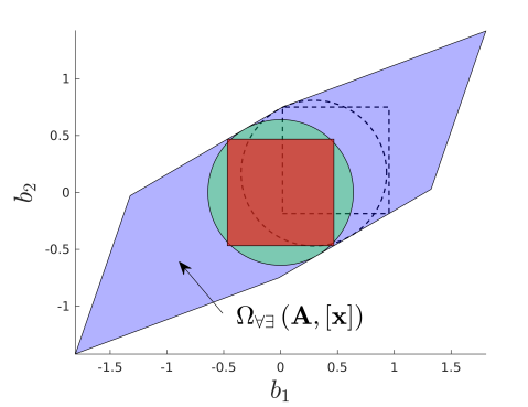
Figure 2: The associated polytope, n-cube, and n-ball inner approximations of $\operatorname{\Omega_{\forall\exists}\left(\operatorname{{\bf A}},[\operatorname{{\bf x}}]\right)}$.

IV-B $\operatorname{\Omega_{\forall\exists}\left([\operatorname{{\bf A}}],[\operatorname{{\bf x}}]\right)}$ Inner Approximations

As stated in (15), the common capabilities are the intersection of the capabilities for all sub-problems $\operatorname{{\bf A}}\in[\operatorname{{\bf A}}]$. Since the capabilities associated with each sub-problem are geometrically convex polytopes, the common capabilities are the intersection of the convex polytopes for all sub-problems.

Theorem 3.

We have $\operatorname{{\bf b}}\in\operatorname{\Omega_{\forall\exists}\left([\operatorname{{\bf A}}],[\operatorname{{\bf x}}]\right)}$ if and only if the linear system

$$\operatorname{{\bf b}}=({\operatorname{mid}\left\lparen[\operatorname{{\bf A}}]\right\rparen}-\operatorname{diag}(\operatorname{{\bf s}})\operatorname{\Delta}[\operatorname{{\bf A}}])\operatorname{{\bf x}}_{1}$$

$$~{}~{}~{}~{}~{}~{}~{}~{}-({\operatorname{mid}\left\lparen[\operatorname{{\bf A}}]\right\rparen}~{}+\operatorname{diag}(\operatorname{{\bf s}})\operatorname{\Delta}[\operatorname{{\bf A}}])\operatorname{{\bf x}}_{2},$$

$$\operatorname{{\bf x}}_{1},\operatorname{{\bf x}}_{2}\geq 0,$$

$$\underline{{\operatorname{{\bf x}}}}\leq\operatorname{{\bf x}}_{1}-\operatorname{{\bf x}}_{2}\leq\overline{{\operatorname{{\bf x}}}}$$

is solvable for each $\operatorname{{\bf s}}\in\{\pm 1\}^{m}$, where $\operatorname{diag}(\operatorname{{\bf s}})$ generates a diagonal matrix from the vector $\operatorname{{\bf s}}$.

Proof.

For a fixed $\operatorname{{\bf b}}$, we have $\operatorname{{\bf b}}\in\operatorname{\Omega_{\forall\exists}\left([\operatorname{{\bf A}}],[\operatorname{{\bf x}}]\right)}$ if and only if the linear system

$$\operatorname{{\bf b}}=\operatorname{{\bf A}}\operatorname{{\bf x}},\ \ \underline{{\operatorname{{\bf x}}}}\leq\operatorname{{\bf x}}\leq\overline{{\operatorname{{\bf x}}}}$$ (28)

is solvable in variable $\operatorname{{\bf x}}$ for each $\operatorname{{\bf A}}\in[\operatorname{{\bf A}}]$. By [32], this kind of strong solvability is equivalent to solvability of the system from the theorem statement. ∎

The above test requires to solve $2^{m}$ linear systems. This can be a large number, however, it can hardly be decreased in general since the problem is intractable.

Theorem 4.

The test $\operatorname{{\bf b}}\in\operatorname{\Omega_{\forall\exists}\left([\operatorname{{\bf A}}],[\operatorname{{\bf x}}]\right)}$ is co-NP-hard.

Proof.

Suppose that $[\operatorname{{\bf x}}]$ is sufficiently large. Then the test $\operatorname{{\bf b}}\in\operatorname{\Omega_{\forall\exists}\left([\operatorname{{\bf A}}],[\operatorname{{\bf x}}]\right)}$ is equivalent to stating that for each $\operatorname{{\bf A}}\in[\operatorname{{\bf A}}]$ there is $\operatorname{{\bf x}}$ such that $\operatorname{{\bf A}}\operatorname{{\bf x}}=\operatorname{{\bf b}}$. That is equivalent with claiming that the interval linear system $[\operatorname{{\bf A}}]\operatorname{{\bf x}}=\operatorname{{\bf b}}$ is strongly solvable. Strong solvability is, however, known to be co-NP-hard [33]. The real valued right-hand side $\operatorname{{\bf b}}$ of the linear system can be easily deduced. ∎

To make the problem tractable, we first construct an inner approximation of $\operatorname{\Omega_{\forall\exists}\left([\operatorname{{\bf A}}],[\operatorname{{\bf x}}]\right)}$ by a zonotope, that is, by a set of the form $\Omega_{\forall\exists}\left(\operatorname{{\bf A}},[\operatorname{{\bf y}}]\right)$ for some $\operatorname{{\bf A}}$ and $[\operatorname{{\bf y}}]$. In particular, we will choose $\operatorname{{\bf A}}:={\operatorname{mid}\left\lparen[\operatorname{{\bf A}}]\right\rparen}$ and $[\operatorname{{\bf y}}]:={\operatorname{mid}\left\lparen[\operatorname{{\bf x}}]\right\rparen}+[-r,r]\operatorname{\Delta}[\operatorname{{\bf x}}]$. The task is now to compute as large as possible value $r\in[0,1]$ such that $\Omega_{\forall\exists}\left({\operatorname{mid}\left\lparen[\operatorname{{\bf A}}]\right\rparen},[\operatorname{{\bf y}}]\right)\subseteq\operatorname{\Omega_{\forall\exists}\left([\operatorname{{\bf A}}],[\operatorname{{\bf x}}]\right)}$. Notice that this need not be satisfied even for $r=0$, so we present a sufficient condition below.

Theorem 5.

Suppose that ${\operatorname{mid}\left\lparen[\operatorname{{\bf A}}]\right\rparen}$ has full row rank and put

$$r=\min_{i=1,\dots,n}\left(\frac{\left(\operatorname{\Delta}[\operatorname{{\bf x}}]-|{\operatorname{mid}\left\lparen[\operatorname{{\bf A}}]\right\rparen}^{\dagger}|\cdot\operatorname{\Delta}[\operatorname{{\bf A}}]\cdot{\operatorname{mag}\left\lparen[\operatorname{{\bf x}}]\right\rparen}\right)_{i}}{\operatorname{\Delta}[\operatorname{{\bf x}}]_{i}}\right),$$ (29)

where $(\cdot)^{{\dagger}}$ denotes the Moore–Penrose pseudoinverse. If $r\geq 0$, then $\Omega_{\forall\exists}\left({\operatorname{mid}\left\lparen[\operatorname{{\bf A}}]\right\rparen},[\operatorname{{\bf y}}]\right)\subseteq\operatorname{\Omega_{\forall\exists}\left([\operatorname{{\bf A}}],[\operatorname{{\bf x}}]\right)}$.

Proof.

We want $\Omega_{\forall\exists}\left({\operatorname{mid}\left\lparen[\operatorname{{\bf A}}]\right\rparen},[\operatorname{{\bf y}}]\right)\subseteq\operatorname{\Omega_{\forall\exists}\left(\operatorname{{\bf A}},[\operatorname{{\bf x}}]\right)}$ for each $\operatorname{{\bf A}}\in[\operatorname{{\bf A}}]$. That is, for each $\operatorname{{\bf y}}\in[\operatorname{{\bf y}}]$ there must be $\operatorname{{\bf x}}\in[\operatorname{{\bf x}}]$ such that ${\operatorname{mid}\left\lparen[\operatorname{{\bf A}}]\right\rparen}\operatorname{{\bf y}}=\operatorname{{\bf A}}\operatorname{{\bf x}}$. Putting $\operatorname{{\bf A}}^{\prime}:={\operatorname{mid}\left\lparen[\operatorname{{\bf A}}]\right\rparen}-\operatorname{{\bf A}}$, we can write it as

$${\operatorname{mid}\left\lparen[\operatorname{{\bf A}}]\right\rparen}\operatorname{{\bf y}}+\operatorname{{\bf A}}^{\prime}\operatorname{{\bf x}}={\operatorname{mid}\left\lparen[\operatorname{{\bf A}}]\right\rparen}\operatorname{{\bf x}}.$$

When $\operatorname{{\bf x}}\in[\operatorname{{\bf x}}]$ and $\operatorname{{\bf A}}\in[\operatorname{{\bf A}}]$, the value of $\operatorname{{\bf A}}^{\prime}\operatorname{{\bf x}}$ ranges in the interval

$$[\operatorname{{\bf z}}]:=[-1,1]\operatorname{\Delta}[\operatorname{{\bf A}}]{\operatorname{mag}\left\lparen[\operatorname{{\bf x}}]\right\rparen}.$$

Thus it is sufficient to find $[\operatorname{{\bf y}}]$ such that

$$\Omega_{\forall\exists}\left({\operatorname{mid}\left\lparen[\operatorname{{\bf A}}]\right\rparen},[\operatorname{{\bf y}}]\right)+[\operatorname{{\bf z}}]\subseteq\Omega_{\forall\exists}\left({\operatorname{mid}\left\lparen[\operatorname{{\bf A}}]\right\rparen},[\operatorname{{\bf x}}]\right).$$

That is, for each $\operatorname{{\bf y}}\in[\operatorname{{\bf y}}]$ and $\operatorname{{\bf z}}\in[\operatorname{{\bf z}}]$, there must be $\operatorname{{\bf x}}\in[\operatorname{{\bf x}}]$ such that

$${\operatorname{mid}\left\lparen[\operatorname{{\bf A}}]\right\rparen}\operatorname{{\bf y}}+\operatorname{{\bf z}}={\operatorname{mid}\left\lparen[\operatorname{{\bf A}}]\right\rparen}\operatorname{{\bf x}},$$

or, equivalently

$$\operatorname{{\bf z}}={\operatorname{mid}\left\lparen[\operatorname{{\bf A}}]\right\rparen}(\operatorname{{\bf x}}-\operatorname{{\bf y}}).$$

If ${\operatorname{mid}\left\lparen[\operatorname{{\bf A}}]\right\rparen}$ has full row rank, this equation can be deduced from

$${\operatorname{mid}\left\lparen[\operatorname{{\bf A}}]\right\rparen}^{\dagger}\operatorname{{\bf z}}=\operatorname{{\bf x}}-\operatorname{{\bf y}}.$$

By choosing an appropriate $\operatorname{{\bf x}}$, the right-hand side can attain any vector in $[-1,1](1-r)\operatorname{\Delta}[\operatorname{{\bf x}}]$. Since the interval vector $[\operatorname{{\bf z}}]$ is symmetric around zero, it is sufficient to compare the radii

$$|{\operatorname{mid}\left\lparen[\operatorname{{\bf A}}]\right\rparen}^{\dagger}|\operatorname{\Delta}[\operatorname{{\bf z}}]\leq(1-r)\operatorname{\Delta}[\operatorname{{\bf x}}],$$

from which the statement follows. ∎

This approach to computing an inner polytope approximation of $\operatorname{\Omega_{\forall\exists}\left([\operatorname{{\bf A}}],[\operatorname{{\bf x}}]\right)}$ by a set of the form $\Omega_{\forall\exists}\left({\operatorname{mid}\left\lparen[\operatorname{{\bf A}}]\right\rparen},[\operatorname{{\bf y}}]\right)$ is particularly convenient when the intervals in $[\operatorname{{\bf A}}]$ are narrow relatively to those in $[\operatorname{{\bf x}}]$. In that case, the value of $r$ is close to 1, and the inner approximation is tight. Inner approximations for the largest inscribed n-ball and n-cube in $\operatorname{\Omega_{\forall\exists}\left([\operatorname{{\bf A}}],[\operatorname{{\bf x}}]\right)}$ may then be computed from the inner polytope approximation $\Omega_{\forall\exists}\left({\operatorname{mid}\left\lparen[\operatorname{{\bf A}}]\right\rparen},[\operatorname{{\bf y}}]\right)$ using Theorems 1 and 2 respectively.

As an example, given $\operatorname{{\bf A}}$ and $[\operatorname{{\bf x}}]$ from (27) and adding uncertainties of $[-0.01,0.01]$ to each matrix element gives the following inner approximation of $\operatorname{\Omega_{\forall\exists}\left([\operatorname{{\bf A}}],[\operatorname{{\bf x}}]\right)}$ shown in Figure 3:

• the associated polytope with $r=0.9289$ (purple);

• the largest n-cube centered at the origin with $r=0.4353$ (red);

• the largest n-ball centered at the origin with $r=0.5951$ (green);

• the largest n-cube with variable center with $b_{c}=(0.4510,0.2622)$ and $r=0.4353$ (dashed line);

• the largest n-ball with variable center with $b_{c}=(0.2714,0.1577)$ and $r=0.5951$ (dashed line).

For comparison the polytope $\operatorname{\Omega_{\forall\exists}\left(mid([\operatorname{{\bf A}}]),[\operatorname{{\bf x}}]\right)}$ is also shown which necessarily contains the polytope $\operatorname{\Omega_{\forall\exists}\left([\operatorname{{\bf A}}],[\operatorname{{\bf x}}]\right)}$ due to (15).

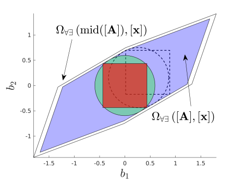
Figure 3: The associated polytope, n-cube, and n-ball inner approximations for $\operatorname{\Omega_{\forall\exists}\left([\operatorname{{\bf A}}],[\operatorname{{\bf x}}]\right)}$. For comparison the polytope $\operatorname{\Omega_{\forall\exists}\left(mid([\operatorname{{\bf A}}]),[\operatorname{{\bf x}}]\right)}$ is also shown.

IV-C Inner Approximations of $\operatorname{\Sigma_{\forall\exists}\left([\operatorname{{\bf A}}],[\operatorname{{\bf b}}]\right)}$

According to [34], a vector $\operatorname{{\bf x}}$ belongs to $\operatorname{\Sigma_{\forall\exists}\left([\operatorname{{\bf A}}],[\operatorname{{\bf b}}]\right)}$ (i.e., is a tolerance solution) if an only if

$$\left|{\operatorname{mid}\left\lparen[\operatorname{{\bf A}}]\right\rparen}\operatorname{{\bf x}}-{\operatorname{mid}\left\lparen[\operatorname{{\bf b}}]\right\rparen}\right|\leq-{\operatorname{\Delta}{[\operatorname{{\bf A}}]}}|\operatorname{{\bf x}}|+{\operatorname{\Delta}{[\operatorname{{\bf b}}]}}$$ (30)

This allows to quickly verify if a desired property exists locally. Furthermore, the following theorems are proposed for directly computing inner approximations of the local capabilities, which may be used for real-time applications. The problems of computing outer approximations of the tolerable solution set have been addressed in [11].

Theorem 6 (Largest inscribed n-cube centered at ${\operatorname{{\bf x}}_{c}}$).

If ${\operatorname{{\bf x}}_{c}}$ belongs to $\operatorname{\Sigma_{\forall\exists}\left([\operatorname{{\bf A}}],[\operatorname{{\bf b}}]\right)}$ then an n-cube

$$~{}[\operatorname{{\bf c}}]={\operatorname{{\bf x}}_{c}}+r[\operatorname{{\bf e}}]$$ (31)

with

$$r=\min_{i=1,\ldots,m}{\operatorname{inf}{\left({\frac{{\operatorname{\Delta}{b_{i}}}-\left|{\operatorname{mid}\left\lparen[b_{i}]\right\rparen}-[\operatorname{{\bf a}}_{i}]{\operatorname{{\bf x}}_{c}}\right|}{\|[\operatorname{{\bf a}}_{i}]\|_{1}}}\right)}}$$ (32)

where $[\operatorname{{\bf a}}_{i}]$ is the $i^{th}$ row of $[\operatorname{{\bf A}}]$, is contained in $\operatorname{\Sigma_{\forall\exists}\left([\operatorname{{\bf A}}],[\operatorname{{\bf b}}]\right)}$.

The proof for Theorem 6 is given in [35]. Notice that it provides the largest n-cube centered in ${\operatorname{{\bf x}}_{c}}$. Notice also that it requires that the right-hand side of (32) is evaluated exactly. If we evaluate it by interval arithmetic, it provides a lower bound on the largest cube only. In [36], the problems of computing inner approximations of the tolerable solution set are also considered.

On the other hand, the test $[\operatorname{{\bf c}}]\subseteq\operatorname{\Sigma_{\forall\exists}\left([\operatorname{{\bf A}}],[\operatorname{{\bf b}}]\right)}$ can be simply performed by interval evaluation $[\operatorname{{\bf A}}][\operatorname{{\bf c}}]\subseteq[\operatorname{{\bf b}}]$. Therefore, we can extend the above inner n-cube $[\operatorname{{\bf c}}]$ by $\varepsilon$-inflation approach to $[\operatorname{{\bf c}}]:=[\operatorname{{\bf c}}]+\varepsilon[\operatorname{{\bf e}}]$ and repeat it while the test does not break.

To overcome the above drawbacks, we propose a more general method. It finds the optimal center point of the n-cube and it computes exactly its radius, too.

Theorem 7 (Largest inscribed n-cube with variable center).

The largest inscribed n-cube to $\operatorname{\Sigma_{\forall\exists}\left([\operatorname{{\bf A}}],[\operatorname{{\bf b}}]\right)}$ reads $[\operatorname{{\bf c}}]=\operatorname{{\bf x}}_{c}+r[\operatorname{{\bf e}}]$, where $\operatorname{{\bf x}}_{c},r$ is an optimal solution to

$$\max\ \ r$$ (33a)

subject to $$\sum_{j}y^{i}_{j}\leq\overline{{b}}_{i},\quad\forall i,$$ (33b)

$$y^{i}_{j}\geq\overline{{a}}_{ij}({x_{c}}_{j}+r),$$ (33c)

$$y^{i}_{j}\geq\overline{{a}}_{ij}({x_{c}}_{j}-r),$$ (33d)

$$y^{i}_{j}\geq\underline{{a}}_{ij}({x_{c}}_{j}+r),$$ (33e)

$$y^{i}_{j}\geq\underline{{a}}_{ij}({x_{c}}_{j}-r),$$ (33f)

$$\sum_{j}z^{i}_{j}\geq\underline{{b}}_{i},\quad\forall i,$$ (33g)

$$z^{i}_{j}\leq\overline{{a}}_{ij}({x_{c}}_{j}+r),$$ (33h)

$$z^{i}_{j}\leq\overline{{a}}_{ij}({x_{c}}_{j}-r),$$ (33i)

$$z^{i}_{j}\leq\underline{{a}}_{ij}({x_{c}}_{j}+r),$$ (33j)

$$z^{i}_{j}\leq\underline{{a}}_{ij}({x_{c}}_{j}-r).$$ (33k)

Proof.

Our problem reads

$$\max\ \ r$$

subject to $${\operatorname{sup}{\left({[\operatorname{{\bf a}}_{i}](\operatorname{{\bf x}}_{c}+r[\operatorname{{\bf e}}])}\right)}}\leq\overline{{b}}_{i}\quad\forall i,$$

$${\operatorname{inf}{\left({[\operatorname{{\bf a}}_{i}](\operatorname{{\bf x}}_{c}+r[\operatorname{{\bf e}}])}\right)}}\geq\underline{{b}}_{i}\quad\forall i.$$

Denoting by $y^{i}_{j}$ and $z^{i}_{j}$ the supremum and the infimum of the product $[a_{ij}]({x_{c}}_{j}+r[-1,1])$, respectively, the resulting optimization model follows. ∎

Notice that (33) is a linear programming problem, so it can be solved efficiently. The number of variables is $1+n+2mn$, so the problem is still polynomially solvable.

Theorem 8 (Largest inscribed n-ball centered at ${\operatorname{{\bf x}}_{c}}$).

If ${\operatorname{{\bf x}}_{c}}$ belongs to $\operatorname{\Sigma_{\forall\exists}\left([\operatorname{{\bf A}}],[\operatorname{{\bf b}}]\right)}$, then the n-ball

$$\mathcal{B}=\{\operatorname{{\bf x}}~{}|~{}\|\operatorname{{\bf x}}-{\operatorname{{\bf x}}_{c}}\|\leq r\}$$ (34)

with

$$r =\min_{i=1,\ldots,m}$$ (35)

$$\operatorname{min}\left({\operatorname{inf}{\left({\frac{-[\operatorname{{\bf a}}_{i}]{\operatorname{{\bf x}}_{c}}+\overline{{b}}_{i}}{\|[\operatorname{{\bf a}}_{i}]\|_{2}}}\right)}},\,{\operatorname{inf}{\left({\frac{[\operatorname{{\bf a}}_{i}]{\operatorname{{\bf x}}_{c}}-\underline{{b}}_{i}}{\|[\operatorname{{\bf a}}_{i}]\|_{2}}}\right)}}\right)$$

where ${\|\cdot\|_{2}}$ is the 2-norm, is contained in $\operatorname{\Sigma_{\forall\exists}\left([\operatorname{{\bf A}}],[\operatorname{{\bf b}}]\right)}$.

Proof.

According to [34], we know that any $\operatorname{{\bf x}}\in\operatorname{\Sigma_{\forall\exists}\left([\operatorname{{\bf A}}],[\operatorname{{\bf b}}]\right)}$ must satisfy

$$\{\operatorname{{\bf A}}\operatorname{{\bf x}}~{}|~{}\operatorname{{\bf A}}\in[\operatorname{{\bf A}}]\}\subseteq[\underline{\operatorname{{\bf b}}},\overline{\operatorname{{\bf b}}}]$$ (36)

Therefore, $\operatorname{\Sigma_{\forall\exists}\left([\operatorname{{\bf A}}],[\operatorname{{\bf b}}]\right)}$ is described by the convex polytope given by the following inequalities

$${\operatorname{sup}{\left({[\operatorname{{\bf a}}_{i}]\operatorname{{\bf x}}}\right)}}\leq\overline{{b}}_{i},$$ (37)

$${\operatorname{sup}{\left({-[\operatorname{{\bf a}}_{i}]\operatorname{{\bf x}}}\right)}}\leq-\underline{{b}}_{i},$$

$$\operatorname{{\bf x}}\in\mathbb{R}^{n}$$

$$i=1,\ldots,m$$

where $\operatorname{sup}$ ensures the inequalities are well-defined. In other words, (37) describes the intersection of a set of half-spaces.

For a given $\operatorname{{\bf A}}\in[\operatorname{{\bf A}}]$, the largest n-ball centered at ${\operatorname{{\bf x}}_{c}}$ and inscribed to $\operatorname{\Sigma_{\forall\exists}\left(\operatorname{{\bf A}},[\operatorname{{\bf b}}]\right)}$ is computed by the linear program

$$\max r$$

subject to $${\operatorname{{\bf a}}_{i}{\operatorname{{\bf x}}_{c}}+r\|\operatorname{{\bf a}}_{i}\|_{2}}\leq\overline{{b}}_{i},\quad\forall i,$$

$${-\operatorname{{\bf a}}_{i}{\operatorname{{\bf x}}_{c}}+r\|\operatorname{{\bf a}}_{i}\|_{2}}\leq-\underline{{b}}_{i},\quad\forall i,$$

$$r\geq 0,$$

from which

$$r=\min_{i=1,\ldots,m}\operatorname{min}\left({\frac{-\operatorname{{\bf a}}_{i}{\operatorname{{\bf x}}_{c}}+\overline{{b}}_{i}}{\|\operatorname{{\bf a}}_{i}\|_{2}}},\,{\frac{\operatorname{{\bf a}}_{i}{\operatorname{{\bf x}}_{c}}-\underline{{b}}_{i}}{\|\operatorname{{\bf a}}_{i}\|_{2}}}\right).$$

Now, for the radius of the largest n-ball centered at ${\operatorname{{\bf x}}_{c}}$ inscribed to $\operatorname{\Sigma_{\forall\exists}\left([\operatorname{{\bf A}}],[\operatorname{{\bf b}}]\right)}$ we just minimize subject to $\operatorname{{\bf a}}_{i}\in[\operatorname{{\bf a}}_{i}]$.

∎

The theorem provides the largest n-ball which is centered in a given point ${\operatorname{{\bf x}}_{c}}$. Notice also that it requires that the right-hand side of (35) is evaluated exactly. If we evaluate it by interval arithmetic, it provides a lower bound on the largest ball only.

Lemma 1.

The function $f(a)=\frac{a^{T}x+b}{\|a\|}$ is quasiconcave on the domain $a\not=0$, $a^{T}x+b\geq 0$.

Proof.

Let $\alpha\geq 0$ be fixed. The set of $a\not=0$ satisfying $f(a)\geq\alpha$ is characterized by

$$a^{T}x+b\geq\alpha\|a\|,$$

which describes a convex set. ∎

The elements of the right-hand side of (35) fulfill the assumptions of the lemma. Since quasiconcave functions attain the minima on the border of the domain, we have the corollary below; the second item follows from the fact that (35) is monotone in some cases.

Corollary 1.

For every $i,j$ we have:

1. The right-hand side of (35) is attained for $a_{ij}\in\{\underline{{a}}_{ij},\overline{{a}}_{ij}\}$.

2. If ${x_{c}}_{j}\geq 0$ and ${a}_{ij}\geq 0$, then we can fix $a_{ij}:=\overline{{a}}_{ij}$ in the first infimum of (35).

3. If ${x_{c}}_{j}\leq 0$ and ${a}_{ij}\leq 0$, then we can fix $a_{ij}:=\underline{{a}}_{ij}$ in the first infimum of (35).

4. If ${x_{c}}_{j}\leq 0$ and ${a}_{ij}\geq 0$, then we can fix $a_{ij}:=\overline{{a}}_{ij}$ in the second infimum of (35).

5. If ${x_{c}}_{j}\geq 0$ and ${a}_{ij}\leq 0$, then we can fix $a_{ij}:=\underline{{a}}_{ij}$ in the second infimum of (35).

Therefore, we may quickly check if ${\operatorname{{\bf x}}_{c}}$ belongs to $\operatorname{\Sigma_{\forall\exists}\left([\operatorname{{\bf A}}],[\operatorname{{\bf b}}]\right)}$ by using (30). If so, the corresponding inscribed n-cube and n-ball are computed directly from (32) and (35) respectively. The proposed theorems are also valid for the $\operatorname{\Sigma_{\forall\exists}\left(\operatorname{{\bf A}},[\operatorname{{\bf b}}]\right)}$ sub-problems.

Theorem 9 (Inscribed n-ball with variable center).

Denote $s_{i}\coloneqq{\operatorname{sup}{\left({\|[\operatorname{{\bf a}}_{i}]\|_{2}}\right)}}$ $\forall i$. Let $r,{\operatorname{{\bf x}}_{c}},\operatorname{{\bf y}}$ be an optimal solution of the linear programming problem

$$\max r$$ (38)

subject to $${\operatorname{mid}\left\lparen\operatorname{{\bf a}}_{i}\right\rparen}\operatorname{{\bf x}}_{c}+{\operatorname{\Delta}{\operatorname{{\bf a}}_{i}}}\operatorname{{\bf y}}+rs_{i}\leq\overline{{b}}_{i},\quad\forall i,$$

$$-{\operatorname{mid}\left\lparen\operatorname{{\bf a}}_{i}\right\rparen}\operatorname{{\bf x}}_{c}+{\operatorname{\Delta}{\operatorname{{\bf a}}_{i}}}\operatorname{{\bf y}}+rs_{i}\leq-\underline{{b}}_{i},\quad\forall i,$$

$$r\geq 0,\ \operatorname{{\bf y}}\geq\operatorname{{\bf x}}_{c},\ \operatorname{{\bf y}}\geq-\operatorname{{\bf x}}_{c}.$$

Then the ball (34) is contained in $\operatorname{\Sigma_{\forall\exists}\left([\operatorname{{\bf A}}],[\operatorname{{\bf b}}]\right)}$.

Proof.

As in the proof of Theorem 8, $\operatorname{\Sigma_{\forall\exists}\left([\operatorname{{\bf A}}],[\operatorname{{\bf b}}]\right)}$ is described by (37). The Chebyshev center ${\operatorname{{\bf x}}_{c}}$ of a polytope can be determined by the linear programming problem which reads

$$\max r$$ (39)

subject to $${\operatorname{sup}{\left({[\operatorname{{\bf a}}_{i}]{\operatorname{{\bf x}}_{c}}+r\|[\operatorname{{\bf a}}_{i}]\|_{2}}\right)}}\leq\overline{{b}}_{i},\quad\forall i,$$

$${\operatorname{sup}{\left({-[\operatorname{{\bf a}}_{i}]{\operatorname{{\bf x}}_{c}}+r\|[\operatorname{{\bf a}}_{i}]\|_{2}}\right)}}\leq-\underline{{b}}_{i},\quad\forall i,$$

$$r\geq 0$$

It is hard to express the suprema explicitly, so we estimate them from above, resulting in a lower bound to the maximum inscribed n-ball

$$\max r$$ (40)

subject to $${\operatorname{sup}{\left({[\operatorname{{\bf a}}_{i}]{\operatorname{{\bf x}}_{c}}}\right)}}+rs_{i}\leq\overline{{b}}_{i},\quad\forall i,$$

$${\operatorname{sup}{\left({-[\operatorname{{\bf a}}_{i}]{\operatorname{{\bf x}}_{c}}}\right)}}+rs_{i}\leq-\underline{{b}}_{i},\quad\forall i,$$

$$r\geq 0$$

Since ${\operatorname{sup}{\left({[\operatorname{{\bf a}}_{i}]{\operatorname{{\bf x}}_{c}}}\right)}}={\operatorname{mid}\left\lparen\operatorname{{\bf a}}_{i}\right\rparen}\operatorname{{\bf x}}_{c}+{\operatorname{\Delta}{\operatorname{{\bf a}}_{i}}}|\operatorname{{\bf x}}_{c}|$, we equivalently have (38), where $\operatorname{{\bf y}}$ substitutes for $|\operatorname{{\bf x}}_{c}|$. ∎

By the first item of Corollary 1, the largest inscribed n-ball is attained for a vertex of $\operatorname{{\bf A}}$. This is true not only for the fixed center $\operatorname{{\bf x}}_{c}$, but even when the center is variable (because we can fix the center at the optimal one). This yields the following method of exponential complexity (with respect to the size of $[\operatorname{{\bf A}}]$). It remains an open question if the problem is computationally tractable or not.

Theorem 10 (Largest inscribed n-ball with variable center).

Let $r,{\operatorname{{\bf x}}_{c}}$ be an optimal solution of the linear programming problem

$$\max r$$ (41)

subject to $$\operatorname{{\bf a}}_{i}\operatorname{{\bf x}}_{c}+r\|\operatorname{{\bf a}}_{i}\|_{2}\leq\overline{{b}}_{i},\quad\forall i,\forall\operatorname{{\bf a}}_{i}\in\operatorname{vert}([\operatorname{{\bf a}}_{i}]),$$

$$-\operatorname{{\bf a}}_{i}\operatorname{{\bf x}}_{c}+r\|\operatorname{{\bf a}}_{i}\|_{2}\leq-\underline{{b}}_{i},\quad\forall i,\forall\operatorname{{\bf a}}_{i}\in\operatorname{vert}([\operatorname{{\bf a}}_{i}]),$$

$$r\geq 0.$$

Then the ball (34) is the largest ball contained in $\operatorname{\Sigma_{\forall\exists}\left([\operatorname{{\bf A}}],[\operatorname{{\bf b}}]\right)}$.

The polytope $\operatorname{\Sigma_{\forall\exists}\left([\operatorname{{\bf A}}],[\operatorname{{\bf b}}]\right)}$ may be represented as the set of all feasible solutions of a linear programming problem. The corresponding linear program (42) was first presented in [37].

Theorem 11.

$\operatorname{{\bf x}}\in\operatorname{\Sigma_{\forall\exists}\left([\operatorname{{\bf A}}],[\operatorname{{\bf b}}]\right)}$ if and only if $\operatorname{{\bf x}}=\operatorname{{\bf x}}_{1}-\operatorname{{\bf x}}_{2}$ is a solution to the system of linear inequalities

$$\overline{{\operatorname{{\bf A}}}}\operatorname{{\bf x}}_{1}-\underline{{\operatorname{{\bf A}}}}\operatorname{{\bf x}}_{2} \leq\overline{{\operatorname{{\bf b}}}}$$ (42)

$$-\underline{{\operatorname{{\bf A}}}}\operatorname{{\bf x}}_{1}+\overline{{\operatorname{{\bf A}}}}\operatorname{{\bf x}}_{2} \leq\underline{{\operatorname{{\bf b}}}}$$

$$\operatorname{{\bf x}}_{1}\geq 0,~{}\operatorname{{\bf x}}_{2} \geq 0$$

The proof for Theorem 11 is given in [37].

For example, given $\operatorname{{\bf A}}$ as the transpose from (27) and adding uncertainties of $[-0.01,0.01]$ to each matrix element and an arbitrary non-symmetric box $[\operatorname{{\bf b}}]$

$$[\operatorname{{\bf b}}]=\begin{pmatrix}[-74.0,95.0]\\ [-24.0,20.0]\\ [-22.0,33.0]\end{pmatrix}$$ (43)

the following inner approximations of $\operatorname{\Sigma_{\forall\exists}\left([\operatorname{{\bf A}}],[\operatorname{{\bf b}}]\right)}$ are given in Figure 4:

• the associated polytope (purple);

• the largest n-cube centered at the origin with $r=18.5082$ (red);

• the largest n-ball centered at the origin with $r=25.3333$ (green);

• the largest n-cube with variable center with $x_{c}=(-1.0599,-3.1972)$ and $r=20.3591$ (dashed line);

• the largest n-ball with variable center with $x_{c}=(-2.5291,-0.6963)$ and $r=27.8666$ (dashed line).

For comparison the polytope $\operatorname{\Sigma_{\forall\exists}\left(mid([\operatorname{{\bf A}}]),[\operatorname{{\bf b}}]\right)}$ is also shown which necessarily contains the polytope $\operatorname{\Sigma_{\forall\exists}\left([\operatorname{{\bf A}}],[\operatorname{{\bf b}}]\right)}$ due to (18).

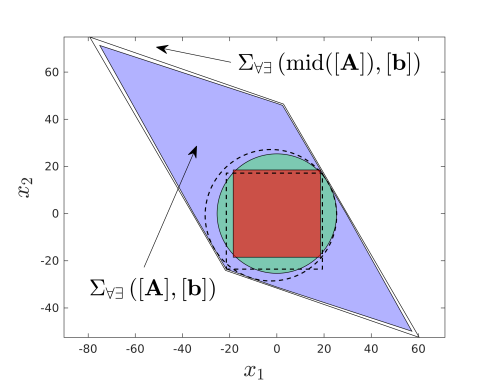
Figure 4: The associated polytope, n-cube, and n-ball inner approximations of $\operatorname{\Sigma_{\forall\exists}\left([\operatorname{{\bf A}}],[\operatorname{{\bf b}}]\right)}$. For comparison the polytope $\operatorname{\Sigma_{\forall\exists}\left(mid([\operatorname{{\bf A}}]),[\operatorname{{\bf b}}]\right)}$ is also shown.

IV-D $\operatorname{\Sigma_{\forall\exists}\left(\operatorname{{\bf A}},[\operatorname{{\bf b}}]\right)}$ Inner Approximations

When $\operatorname{{\bf A}}$ is square, the $\operatorname{\Sigma_{\forall\exists}\left(\operatorname{{\bf A}},[\operatorname{{\bf b}}]\right)}$ polytope can be obtained as the convex hull of the set of $\operatorname{{\bf x}}$ associated with the $2^{m}$ vertices of $[\operatorname{{\bf b}}]$ as

$$\operatorname{\Sigma_{\forall\exists}\left(\operatorname{{\bf A}},[\operatorname{{\bf b}}]\right)}=\operatorname{conv}(\{\operatorname{{\bf x}}~{}|~{}(\exists\operatorname{{\bf b}}\in\operatorname{vert}([\operatorname{{\bf b}}]))(\operatorname{{\bf x}}=\operatorname{{\bf A}}^{-1}\operatorname{{\bf b}})\})$$ (44)

When $\operatorname{{\bf A}}$ is non-square and $m>n$ the linear system of equations is over-determined and the Moore–Penrose pseudoinverse solution

$$\operatorname{{\bf x}}=\operatorname{{\bf A}}^{{\dagger}}\operatorname{{\bf b}},$$ (45)

where $\operatorname{{\bf A}}^{{\dagger}}=(\operatorname{{\bf A}}^{T}\operatorname{{\bf A}})^{-1}\operatorname{{\bf A}}^{T}$, only ensures that the norm of the error $\operatorname{{\bf b}}-\operatorname{{\bf A}}\operatorname{{\bf x}}$ is minimized. This error is zero and (45) has a solution if and only if the set of $\operatorname{{\bf b}}$ belongs to the image ($\operatorname{Im}$) of $\operatorname{{\bf A}}$. In [38] the authors propose finding a reduced polytope that is given by the intersection $[\operatorname{{\bf b}}]\cap\operatorname{Im}(\operatorname{{\bf A}})$ and apply this method to solve the wrench problem of redundant serial manipulators. This approach has been recently extended to allow for online computation of the polytope [39]. For many robotics applications, this is equivalent to considering only the set of $\operatorname{{\bf b}}$ that do not cause internal motions. For example, when considering the velocity kinematics model, only the joint states resulting in motions at the end-effector are considered, as states in the null space produce only internal motions.

The associated $\operatorname{{\bf x}}$ for each vertex of the reduced polytope can be computed from (45) and the convex hull of the resulting set gives the polytope $\operatorname{\Sigma_{\forall\exists}\left(\operatorname{{\bf A}},[\operatorname{{\bf b}}]\right)}$. The $\operatorname{\Sigma_{\forall\exists}\left(\operatorname{{\bf A}},[\operatorname{{\bf b}}]\right)}$ polytope for over-determined systems is given by

$$\operatorname{\Sigma_{\forall\exists}\left(\operatorname{{\bf A}},[\operatorname{{\bf b}}]\right)}=$$ (46)

$$\operatorname{conv}(\{\operatorname{{\bf x}}~{}|~{}(\exists\operatorname{{\bf b}}\in\operatorname{vert}([\operatorname{{\bf b}}]\cap\operatorname{Im}(\operatorname{{\bf A}})))(\operatorname{{\bf x}}=\operatorname{{\bf A}}^{{\dagger}}\operatorname{{\bf b}})\})$$

The proposed n-cube and n-ball theorems (Theorems 6, 7, and 8) are also valid and applicable to the $\operatorname{\Sigma_{\forall\exists}\left(\operatorname{{\bf A}},[\operatorname{{\bf b}}]\right)}$ sub-problems.

For example, given $\operatorname{{\bf A}}$ as the transpose from (27) and $[\operatorname{{\bf b}}]$ from (43), the box $[\operatorname{{\bf b}}]$ and corresponding reduced polytope $[\operatorname{{\bf b}}]\cap\operatorname{Im}(\operatorname{{\bf A}})$, and the following inner approximations of $\operatorname{\Sigma_{\forall\exists}\left(\operatorname{{\bf A}},[\operatorname{{\bf b}}]\right)}$ are given in Figure 5:

• the associated polytope (purple);

• the largest n-cube centered at the origin with $r=18.8573$ (red);

• the largest n-ball centered at the origin with $r=25.7800$ (green);

• the largest n-cube with variable center with $x_{c}=(-1.0450,-3.3319)$ and $r=20.7430$ (dashed line);

• the largest n-ball with variable center with $x_{c}=(-2.5624,-0.7216)$ and $r=28.3579$ (dashed line).

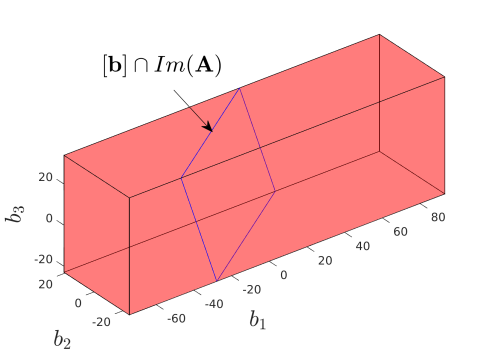
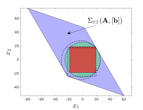
Figure 5: (Top) The box $[\operatorname{{\bf b}}]$ and the corresponding reduced polytope $[\operatorname{{\bf b}}]\cap\operatorname{Im}(\operatorname{{\bf A}})$. (Bottom) The associated polytope, n-cube, and n-ball inner approximations of $\operatorname{\Sigma_{\forall\exists}\left(\operatorname{{\bf A}},[\operatorname{{\bf b}}]\right)}$.

IV-E Inner Approximations Summary

The equations associated with each inner approximation for each class of problem are summarized in Table III. Software implementations of the proposed inner approximation algorithms are made available at [40] for Matlab. To get an estimate of the computational times for typical 7-degree-of-freedom redundant robotics applications, for each problem the mean computational times and standard deviations (over 20 runs) evaluated for a random system with $n=7$ and $m=6$ are provided in Table III. The fixed center point is taken as the origin. It can be noted that the Matlab implementations are not optimized for speed and the computational times can be significantly reduced with more efficient implementations. However, the already low computational times for many of the inner approximations demonstrates the suitability for real-time applications.

TABLE III: Inner approximation summary.

Approximations	$\operatorname{\Omega_{\forall\exists}\left(\operatorname{{\bf A}},[\operatorname{{\bf x}}]\right)}$	ms $\pm$ std	$\operatorname{\Omega_{\forall\exists}\left([\operatorname{{\bf A}}],[\operatorname{{\bf x}}]\right)}$	ms $\pm$ std	$\operatorname{\Sigma_{\forall\exists}\left(\operatorname{{\bf A}},[\operatorname{{\bf b}}]\right)}$	ms $\pm$ std	$\operatorname{\Sigma_{\forall\exists}\left([\operatorname{{\bf A}}],[\operatorname{{\bf b}}]\right)}$	ms$\pm$ std
Polytope inner	(19)	56.842	(29) + (19)	56.719	(44) or (46)	187.374	(42)	381.568
approximation		$\pm$1.090		$\pm$0.430		$\pm$0.982		$\pm$3.544
Largest inscribed n-cube	(19) + (22)	1.496	(29) + (22)	1.537	(32)	0.024	(32)	0.024
centered at a point		$\pm$0.033		$\pm$0.030		$\pm$0.002		$\pm$0.001
Largest inscribed n-cube	(19) + (23)	20.748	(29) + (23)	20.807	(33) – exact	30.690	(33) – exact	33.154
with variable center		$\pm$0.389		$\pm$0.310		$\pm$0.414		$\pm$0.675
Largest inscribed n-ball	(19) + (25)	1.509	(29) + (25)	1.541	(35)	0.036	(35)	0.036
centered at a point		$\pm$0.029		$\pm$0.023		$\pm$0.004		$\pm$0.002
Largest inscribed n-ball	(19) + (26)	19.872	(29) + (26)	19.883	(38)	17.287	(38)	17.560
with variable center		$\pm$0.322		$\pm$0.294		$\pm$0.181		$\pm$0.434
					(41) – exact	34.701	(41) – exact	48.459
						$\pm$ 0.466		$\pm$0.481

V Applications

One application of this work is to improve the reliability of the computed capabilities, since all sources of error can be easily modeled and managed. Methods for reliably modeling sources of error are described within the appropriate design framework [21, 41]. This allows to compute certifiable results providing confidence of the calculated capabilities of a manipulator. Other applications of this work are to provide reliable inner approximations of the common capabilities of a robotic manipulator over a given time horizon. This allows to reliably compute local capabilities, in real-time in many cases, that can be used online to evaluate the manipulator’s current capabilities as well as its future capabilities within a time horizon.

As a simple example, consider a redundant three-link planar manipulator for a positioning task with point masses $m_{1},m_{2},m_{3}$ at distal ends of links of lengths $l_{1},l_{2},l_{3}$. The manipulator is depicted in Figure 6.

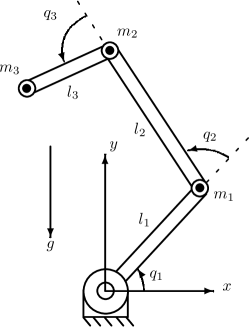
Figure 6: Three-link planar manipulator with point masses at distal ends of links.

The manipulator’s $2\times 3$ Jacobian matrix is given by

$${\operatorname{{\bf J}}}(\operatorname{{\bf q}})= \begin{pmatrix}J_{1}-sq_{12}l_{2}-sq_{1}l_{1}&J_{1}-sq_{12}l_{2}&J_{1}\\ J_{2}+cq_{12}l_{2}+cq_{1}l_{1}&J_{2}+cq_{12}l_{2}&J_{2}\\ \end{pmatrix}$$ (47)

where $q_{ijk}=(q_{i}+q_{j}+q_{k})$, $sq_{i}=\sin(q_{i})$, $cq_{i}=\cos(q_{i})$, $J_{1}=-sq_{123}l_{3}$, and $J_{2}=cq_{123}l_{3}$.

The $2\times 3$ time derivative of the Jacobian matrix is given by

$$\dot{\operatorname{{\bf J}}}(\operatorname{{\bf q}},\dot{\operatorname{{\bf q}}})= \begin{pmatrix}-J_{6}-J_{3}-cq_{1}l_{1}\dot{q}_{1}&-J_{6}-J_{3}&-J_{6}\\ J_{5}-J_{4}-sq_{1}l_{1}\dot{q}_{1}&J_{5}-J_{4}&J_{5}\\ \end{pmatrix}$$ (48)

where $\dot{q}_{ijk}=\dot{q}_{i}+\dot{q}_{j}+\dot{q}_{k}$, $J_{3}=cq_{12}l_{2}\dot{q}_{12}$, $J_{4}=sq_{12}l_{2}\dot{q}_{12}$, $J_{5}=J_{1}\dot{q}_{123}$, and $J_{6}=J_{2}\dot{q}_{123}$.

The mass matrix, centrifugal and Coriolis vector, and gravity vector are given by

$${\bf M}(\operatorname{{\bf q}})= \begin{pmatrix}K_{7}&K_{1}+K_{3}+K_{4}&K_{2}+K_{6}\\ K_{1}+K_{3}+K_{4}&2K_{5}+K_{4}&K_{5}+K_{6}\\ K_{2}+K_{6}&K_{5}+K_{6}&K_{6}\\ \end{pmatrix}$$ (49)

$${\bf c}(\operatorname{{\bf q}},\dot{\operatorname{{\bf q}}})= \begin{pmatrix}K_{10}(K_{8}+K_{12})+K_{11}(K_{8}+K_{9})\\ \dot{q_{1}}^{2}(K_{8}+K_{12})+K_{9}K_{11}\\ -K_{9}K_{10}+\dot{q_{1}}^{2}(K_{8}+K_{9})\\ \end{pmatrix}$$

$${\operatorname{{\bf g}}}(\operatorname{{\bf q}})= g\begin{pmatrix}cq_{123}l_{3}m_{3}+l_{2}cq_{12}m_{23}+l_{1}cq_{1}m_{123}\\ cq_{123}l_{3}m_{3}+l_{2}cq_{12}m_{23}\\ cq_{123}l_{3}m_{3}\\ \end{pmatrix}$$

where

$$K_{1} =l_{1}l_{2}m_{23}cq_{2}$$ (50)

$$K_{2} =l_{3}m_{3}(l_{1}cq_{23}+l_{2}cq_{3})$$

$$K_{3} =l_{3}m_{3}(l_{1}cq_{23}+2l_{2}cq_{3})$$

$$K_{4} =l_{2}^{2}m_{23}+K_{6}$$

$$K_{5} =l_{2}l_{3}m_{3}cq_{3}$$

$$K_{6} =l_{3}^{2}m_{3}$$

$$K_{7} =2K_{1}+2K_{2}+K_{4}+l_{1}^{2}m_{123}$$

$$K_{8} =l_{1}l_{3}m_{3}sq_{23}$$

$$K_{9} =l_{2}l_{3}m_{3}sq_{3}$$

$$K_{10} =-(2\dot{q}_{1}\dot{q}_{2}+\dot{q}_{2}^{2})$$

$$K_{11} =-(2\dot{q}_{1}\dot{q}_{3}+2\dot{q}_{2}\dot{q}_{3}+\dot{q}_{3}^{2})$$

$$K_{12} =l_{1}l_{2}m_{23}sq_{2}$$

with $m_{ijk}=m_{i}+m_{j}+m_{k}$, and $g$ is the gravitational constant.

For the following examples, realistic parameters and joint state limits are selected to approximate a simplified planar model of joints 2, 4, and 6 of the Franka Emika Panda robot. The parameter values with assumed uncertainties are

$$=0.328\pm 0.0001~{}\text{m}$$ (51)

$$[l_{2}] =0.394\pm 0.0001~{}\text{m}$$

$$[l_{3}] =0.1385\pm 0.0001~{}\text{m}$$

$$[m_{1}] =1.9\pm 0.001~{}\text{kg}$$

$$[m_{2}] =1.6\pm 0.001~{}\text{kg}$$

$$[m_{3}] =1.3\pm 0.001~{}\text{kg}$$

and the corresponding joint state limits (i.e., $[{\operatorname{{\bf q}}}_{lim}]$, $[\dot{\operatorname{{\bf q}}}_{lim}]$, $[\ddot{\operatorname{{\bf q}}}_{lim}]$, $[\boldsymbol{\tau}_{lim}]$, $[\dot{\boldsymbol{\tau}}_{lim}]$) are taken from the manufacturer’s specifications as

$$[{\operatorname{{\bf q}}}_{lim}] =\begin{pmatrix}[-1.7628,1.7628]\\ [-3.0718,-0.0698]\\ [-0.0175,3.7525]\end{pmatrix}~{}\text{rad}$$ (52)

$$[\dot{\operatorname{{\bf q}}}_{lim}] =\begin{pmatrix}[-2.175,2.175]\\ [-2.175,2.175]\\ [-2.610,2.610]\end{pmatrix}~{}\text{rad/s}$$

$$[\ddot{\operatorname{{\bf q}}}_{lim}] =\begin{pmatrix}[-7.5,7.5]\\ [-12.5,12.5]\\ [-20,20]\end{pmatrix}~{}\text{rad/s}^{2}$$

$$[\boldsymbol{\tau}_{lim}] =\begin{pmatrix}[-87,87]\\ [-87,87]\\ [-12,12]\end{pmatrix}~{}\text{Nm}$$

$$[\dot{\boldsymbol{\tau}}_{lim}] =\begin{pmatrix}[-1000,1000]\\ [-1000,1000]\\ [-1000,1000]\end{pmatrix}~{}\text{Nm/s}$$

To visualize the effects of considering a set of configurations, for

$$[{\operatorname{{\bf q}}}] =(1.0,-1.0,1.0)\pm 0.1~{}\text{rads}$$ (53)

an approximation of the set of positions associated with the distal ends of the links is depicted in Figure 1. The proposed inner approximations provide a convenient means of evaluating the robot’s common capabilities over the corresponding set of poses, provided that the intersection of capabilities is not empty.

V-A Evaluating the Velocity Problem

A necessary procedure when analyzing the performance of a robotic manipulator is to evaluate the possible end-effector velocities through the mapping of known joint velocity limits with (2). The velocity problem is of the class $\operatorname{\Omega_{\forall\exists}\left(\operatorname{{\bf A}},[\operatorname{{\bf x}}]\right)}$ and the associated inner approximations of section IV-A may be used to evaluate the possible end-effector velocities of the manipulator at a given configuration ${\operatorname{{\bf q}}}$. When considering a set of configurations $[{\operatorname{{\bf q}}}]$, the manipulator’s Jacobian matrix becomes an interval matrix and the associated inner approximations of section IV-B may be used.

At the following configurations

$$[{\operatorname{{\bf q}}}] =(0.0,-1.5708,1.8675)\pm 0.01~{}\text{rads}$$ (54)

and with the joint velocities $[\dot{\operatorname{{\bf q}}}]=[\dot{\operatorname{{\bf q}}}_{lim}]$ the inner approximations – associated polytope with $r=0.9136$, largest n-cube centered at the origin with $r=0.4748$ m/s, and largest n-ball centered at the origin with $r=0.6657$ m/s approximations of $\Omega_{\forall\exists}\left({\operatorname{{\bf J}}}([{\operatorname{{\bf q}}}]),[\dot{\operatorname{{\bf q}}}]\right)$ – are given in Figure 7.

Analysis of the manipulator’s velocity capabilities is performed by bisecting the joint configuration space (given in terms of an interval vector $[\operatorname{{\bf q}}]$) into a set of $k$ sub-intervals $[\operatorname{{\bf q}}_{1}],\ldots,[\operatorname{{\bf q}}_{k}]$ at a desired resolution. Each sub-interval is used to evaluate an inner approximation of the corresponding n-ball centered at the origin, thus the continuous configuration space is completely explored without sampling. Plots of the values of $r$ throughout the configuration space (see Figure 7) can be quickly generated and due to the independence of each sub-interval the performance can benefit significantly from parallel computing. Furthermore, if given a desired velocity capability, a branch-and-bound loop can iteratively refine the joint configuration space $[\operatorname{{\bf q}}]$ finding all satisfying configurations for a desired resolution. This has applications for trajectory planning in the redundant configuration space, where feasibility requires a connected path of satisfying configurations and planning involves selection of an optimal path [42]. Note that the use of outer approximations of the manipulator’s velocity capabilities, which are outside of the scope of this current work, can provide a complementary test allowing to quickly remove non-satisfying configurations from the branch-and-bound loop.

Considering the relationship between the velocity kinematics model (2) and manipulability, the largest n-cube and n-ball inner approximations can be used to rapidly evaluate manipulability measures that correspond to given sets of robot states.

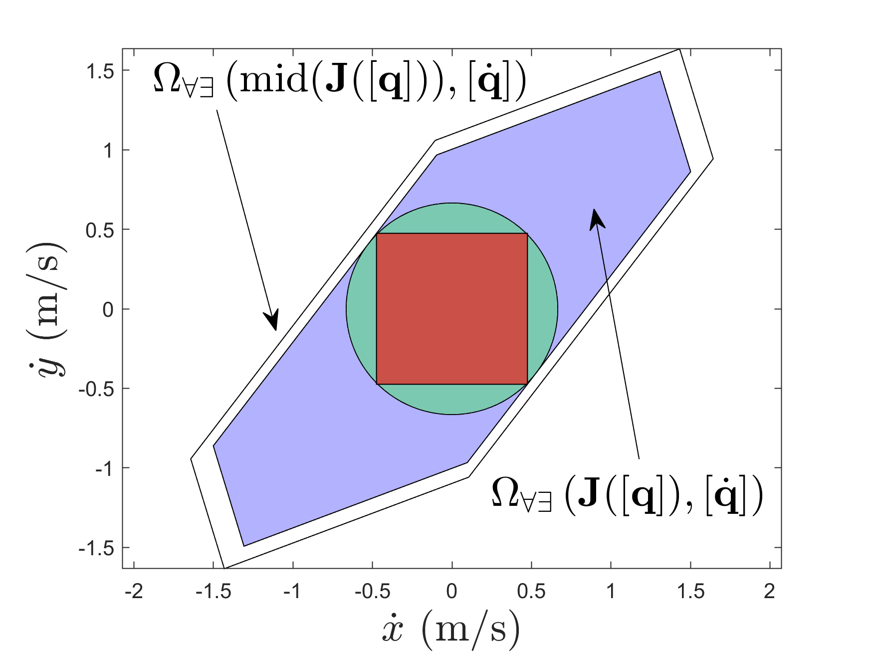
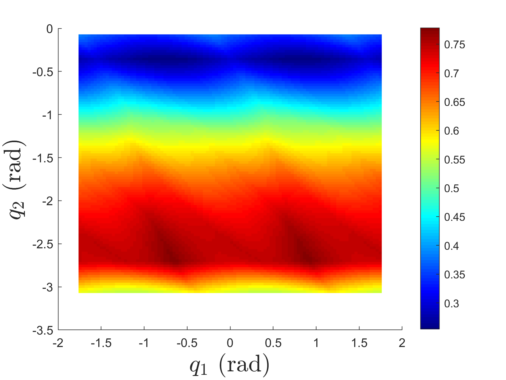
Figure 7: (Top) The associated polytope, largest n-cube centered at the origin, and largest n-ball centered at the origin for the example velocity problem $\Omega_{\forall\exists}\left({\operatorname{{\bf J}}}([{\operatorname{{\bf q}}}]),[\dot{\operatorname{{\bf q}}}]\right)$. (Bottom) A plot of the values of $r$ throughout the configuration space (with $[{q}_{3}]=1.8675\pm 0.01~{}\text{rads}$) for the largest n-ball centered at the origin.

V-B Evaluating the Kinetostatic Problem

Another necessary procedure when analyzing the performance of a robotic manipulator is to evaluate the possible end-effector wrenches through the mapping of known joint torque/force limits with (3). The kinetostatic problem is of the class $\operatorname{\Sigma_{\forall\exists}\left(\operatorname{{\bf A}},[\operatorname{{\bf b}}]\right)}$ and the associated inner approximations of section IV-D may be used to evaluate the possible end-effector wrenches of the manipulator at a given configuration ${\operatorname{{\bf q}}}$. For a set of configurations $[{\operatorname{{\bf q}}}]$, the kinetostatic problem is of the class $\operatorname{\Sigma_{\forall\exists}\left([\operatorname{{\bf A}}],[\operatorname{{\bf b}}]\right)}$ and the associated inner approximations of section IV-C may be used.

At the same configurations (54) and with the joint torques $[\boldsymbol{\tau}]=[\boldsymbol{\tau}_{lim}]$, the inner approximations – associated polytope, largest n-cube centered at the origin with $r=67.3479$ N, and largest n-ball centered at the origin with $r=85.1640$ N approximations of $\Sigma_{\forall\exists}\left({\operatorname{{\bf J}}}([{\operatorname{{\bf q}}}])^{T},[\boldsymbol{\tau}]\right)$ – are given in Figure 8. In addition, the joint configuration space is bisected into sub-intervals and inner approximations of the corresponding n-ball centered at the origin allow to analyze the manipulator’s force capabilities.

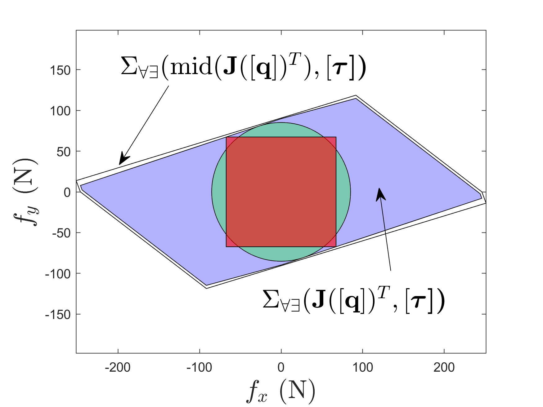
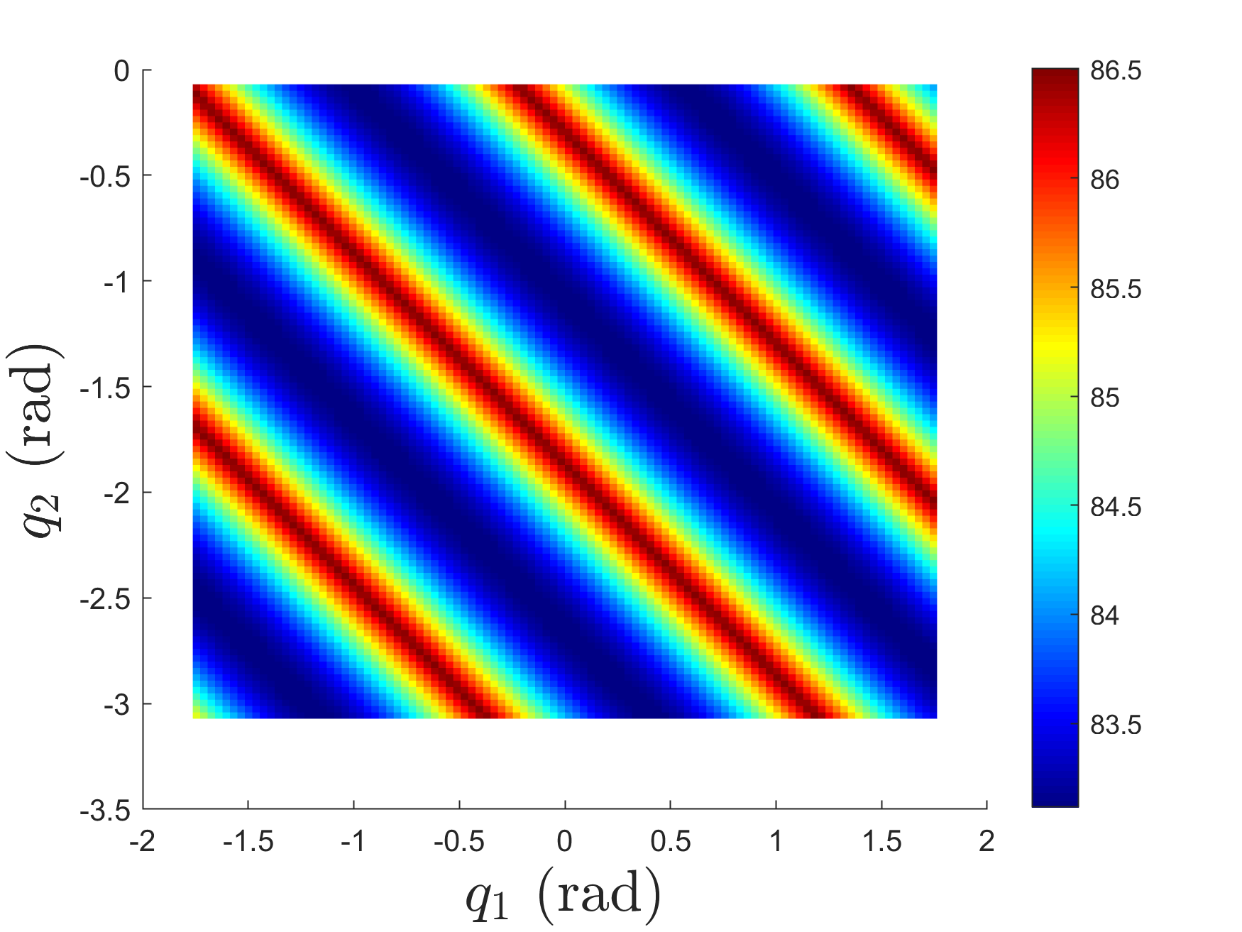
Figure 8: (Top) The associated polytope, largest n-cube centered at the origin, and largest n-ball centered at the origin for the example kinetostatic problem $\Sigma_{\forall\exists}\left({\operatorname{{\bf J}}}([{\operatorname{{\bf q}}}])^{T},[\boldsymbol{\tau}]\right)$. (Bottom) A plot of the values of $r$ throughout the configuration space (with $[{q}_{3}]=1.8675\pm 0.01~{}\text{rads}$) for the largest n-ball centered at the origin.

V-C Evaluating the Forward Acceleration Problem

The local operational acceleration capabilities can be determined from the forward acceleration model (4). The problem can be split into two interval linear systems of equations where each system needs to be solved to give a corresponding set of operational accelerations (see Tables I). The Minkowski sum of the two sets then gives the local operational acceleration capabilities. Inner polytope approximations of the two sets of class $\operatorname{\Omega_{\forall\exists}\left(\operatorname{{\bf A}},[\operatorname{{\bf x}}]\right)}$ or $\operatorname{\Omega_{\forall\exists}\left([\operatorname{{\bf A}}],[\operatorname{{\bf x}}]\right)}$ are obtained from:

$$\ddot{\operatorname{{\bf x}}}_{1} =\dot{\operatorname{{\bf J}}}({\operatorname{{\bf q}}},\dot{\operatorname{{\bf q}}})\dot{\operatorname{{\bf q}}}$$ (55)

$$\ddot{\operatorname{{\bf x}}}_{2} ={\operatorname{{\bf J}}}({\operatorname{{\bf q}}})\ddot{\operatorname{{\bf q}}}$$

Since each inner polytope approximation is convex, the Minkowski sum of the two sets is easily computed as the convex hull of all combinations of polytope vertices. The inner approximations (22) and (25) can then be applied.

Let $\dot{\operatorname{{\bf J}}}({\operatorname{{\bf q}}},\dot{\operatorname{{\bf q}}})$ and ${\operatorname{{\bf J}}}({\operatorname{{\bf q}}})$ be evaluated at the same configurations (54) and with the joint velocities

$$[\dot{\operatorname{{\bf q}}}]=(1.0,1.0,1.0)\pm 0.01~{}\text{rads/s}\\$$ (56)

As more uncertainties or variabilities in the system are considered, the greater the widths of the intervals in the matrices $[\operatorname{{\bf A}}]$ become and therefore the greater the widths of the vectors $[\operatorname{{\bf x}}]$ must be to in order to determine an inner polytope approximation with $r$ greater than zero. Considering the joint state limits $[\dot{\operatorname{{\bf q}}}_{lim}]$ and $[\ddot{\operatorname{{\bf q}}}_{lim}]$, the resulting inner polytope approximations of $\Omega_{\forall\exists}(\dot{\operatorname{{\bf J}}}([{\operatorname{{\bf q}}}],[\dot{\operatorname{{\bf q}}}]),[\dot{\operatorname{{\bf q}}}_{lim}])$ and $\Omega_{\forall\exists}({\operatorname{{\bf J}}}([{\operatorname{{\bf q}}}]),[\ddot{\operatorname{{\bf q}}}_{lim}])$ are $r=0.8446$ and $r=0.9237$, respectively (see Figure 9 top). The inner approximations of the operational acceleration capabilities is Minkowski sum of the two sets (see Figure 9 bottom) with: largest n-cube centered at the origin with $r=5.7386$ m/s², and largest n-ball centered at the origin with $r=7.7526$ m/s². While uncertainties may be largely ignored from a control point of view, accounting for these uncertainties is the only way to truly certify the capabilities of the system.

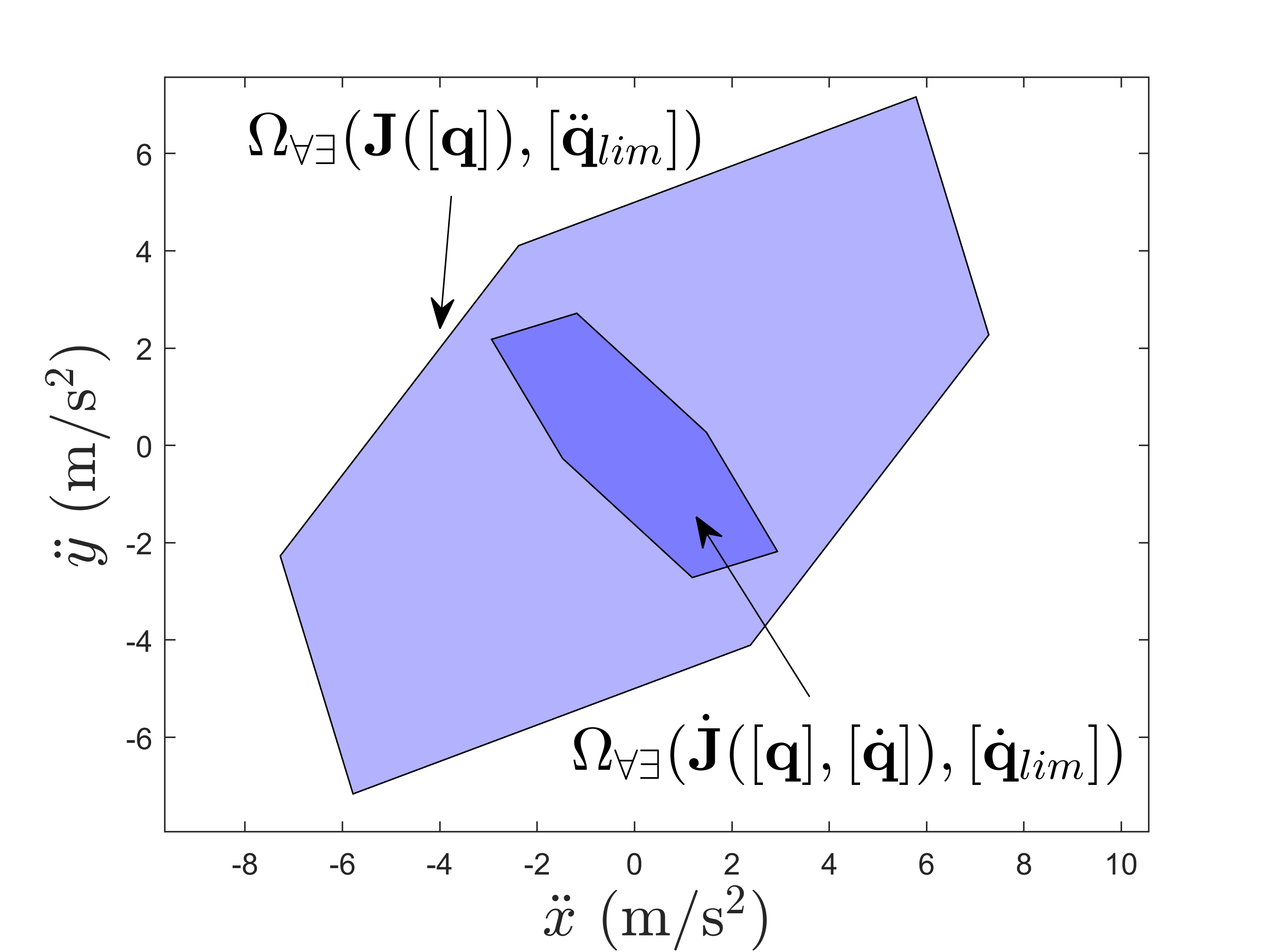
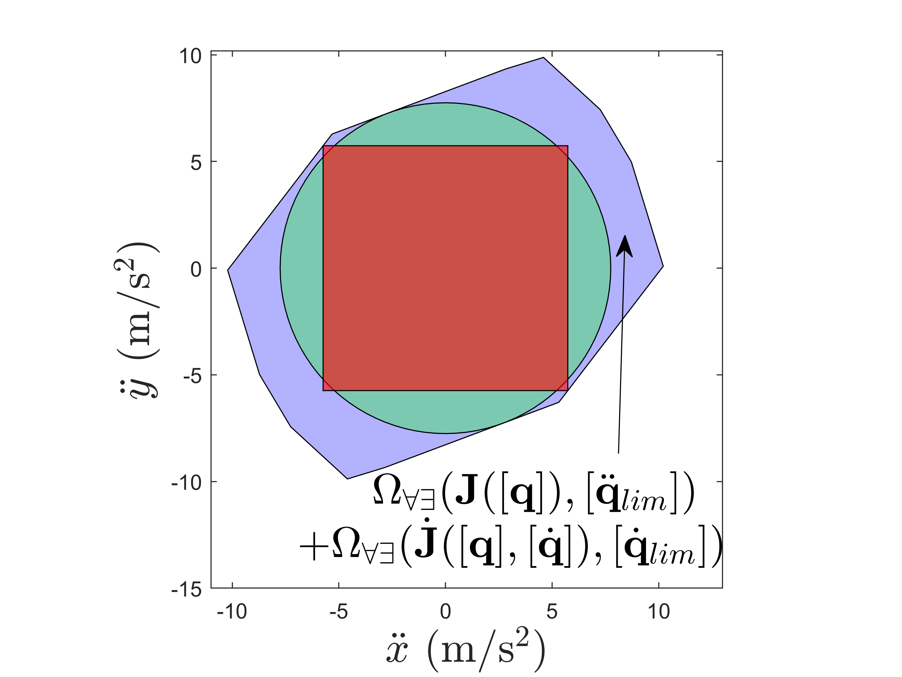
Figure 9: (Top) The associated inner polytope approximations for $\Omega_{\forall\exists}(\dot{\operatorname{{\bf J}}}({\operatorname{{\bf q}}},\dot{\operatorname{{\bf q}}}),[\dot{\operatorname{{\bf q}}}_{lim}])$ and $\Omega_{\forall\exists}({\operatorname{{\bf J}}}({\operatorname{{\bf q}}}),[\ddot{\operatorname{{\bf q}}}_{lim}])$. (Bottom) The associated inner approximations for $\Omega_{\forall\exists}(\dot{\operatorname{{\bf J}}}({\operatorname{{\bf q}}},\dot{\operatorname{{\bf q}}}),[\dot{\operatorname{{\bf q}}}_{lim}])+\Omega_{\forall\exists}({\operatorname{{\bf J}}}({\operatorname{{\bf q}}}),[\ddot{\operatorname{{\bf q}}}_{lim}])$.

V-D Evaluating Future Dynamic Capabilities

Let the current state of a robot be given by $\{\operatorname{{\bf q}},\dot{\operatorname{{\bf q}}},\boldsymbol{\tau}\}$ and let the joint state limits be given by the intervals $\{[\operatorname{{\bf q}}_{lim}],[\dot{\operatorname{{\bf q}}}_{lim}],[\boldsymbol{\tau}_{lim}]\}$ and the control limit be given by the interval $[\dot{\boldsymbol{\tau}}_{lim}]$. Consider a prediction period interval $[t]=[0,t_{max}]$. The future joint torques $[\boldsymbol{\tau}_{f}]$ are bounded by

$$[\boldsymbol{\tau}_{f}]=\left(\boldsymbol{\tau}+[\dot{\boldsymbol{\tau}}_{lim}][t]\right)\cap[\boldsymbol{\tau}_{lim}]$$ (57)

The future joint accelerations $[\ddot{\operatorname{{\bf q}}}_{f}]$ are estimated from joint torque at the current state by

$$[\ddot{\operatorname{{\bf q}}}_{f}]={\bf M}({\operatorname{{\bf q}}})^{-1}\left([\boldsymbol{\tau}_{f}]-\operatorname{{\bf c}}({\operatorname{{\bf q}}},\dot{{\operatorname{{\bf q}}}})-{\operatorname{{\bf g}}}({\operatorname{{\bf q}}})\right).$$ (58)

The future joint velocities $[\dot{\operatorname{{\bf q}}}_{f}]$ are given by

$$[\dot{\operatorname{{\bf q}}}_{f}]=\left(\dot{\operatorname{{\bf q}}}+[\ddot{\operatorname{{\bf q}}}_{{f}}][t]\right)\cap[\dot{\operatorname{{\bf q}}}_{lim}].$$ (59)

The future joint configurations $[\boldsymbol{{{\operatorname{{\bf q}}}}}_{f}]$ are given by

$$[\boldsymbol{{{\operatorname{{\bf q}}}}}_{f}]=\left(\boldsymbol{{{\operatorname{{\bf q}}}}}+[\dot{\operatorname{{\bf q}}}_{f}][t]+\frac{1}{2}[\ddot{\operatorname{{\bf q}}}_{{f}}][t]^{2}\right)\cap[\boldsymbol{{{\operatorname{{\bf q}}}}}_{lim}].$$ (60)

The joint state limit intersections ensure that the limits are not exceeded during the prediction of the future set of states.

It is clear that joint acceleration capabilities are state dependent and therefore if constant joint acceleration limits are enforced, the controller may either require infeasible accelerations from the system or sub-optimally use its actual capabilities. Furthermore, due to the noise associated with the estimation of the current $\ddot{\operatorname{{\bf q}}}$, enforcing constant joint acceleration limits is difficult in practice. Alternatively, the use of joint torques to evaluate joint acceleration capabilities can provide a much better estimate of the capabilities of the system.

The joint acceleration capabilities achievable during the prediction period $[t]$ can be determined from the configuration-space dynamic model (5). However, the right hand side of (5) should not be overestimated. Therefore, let the effective joint torques be given by $[\boldsymbol{\tau}_{e}]=[\underline{\boldsymbol{\tau}_{f}}+\overline{\bf cg},\overline{\boldsymbol{\tau}_{f}}+\underline{\bf cg}]$, where $[{\bf cg}]=-{\operatorname{{\bf c}}}([{\operatorname{{\bf q}}}_{f}],[\dot{\operatorname{{\bf q}}}_{f}])-{\operatorname{{\bf g}}}([{\operatorname{{\bf q}}}_{f}])$. Inner approximations of the joint acceleration capabilities are then computed from

$${\bf M}([{\operatorname{{\bf q}}}_{f}])\ddot{\operatorname{{\bf q}}}=[\boldsymbol{\tau}_{e}].$$ (61)

The problem is of class $\operatorname{\Sigma_{\forall\exists}\left([\operatorname{{\bf A}}],[\operatorname{{\bf b}}]\right)}$ and the associated inner approximations of section IV-C may be used.

As an example, let the current states be given by (54) and (56) and

$$\boldsymbol{\tau}=(18.0,1.0,2.0)~{}\pm 0.01~{}\text{Nm}\\$$ (62)

Selecting the time $[t]=[0,0.01]$ s, the corresponding joint acceleration inner approximation polytope, the largest n-cube centered at the origin with $r=2.3382~{}\text{rad/s}^{2}$, and the largest n-ball centered at the origin with $r=3.2315~{}\text{rad/s}^{2}$ are shown in Figure 10. For visibility reasons only, the polytope is bounded by the manufacturer’s limits $[\ddot{\operatorname{{\bf q}}}_{lim}]$.

The inner polytope approximation of the joint acceleration capabilities represents a set of valid joint accelerations which better describe the future operational accelerations during a prediction period $[t]$. This can be used in the form of inequality constraints inside the robot controller, augmenting the manufacturer’s default limits, to ensure that the robot’s capabilities are properly considered to select valid control actions.

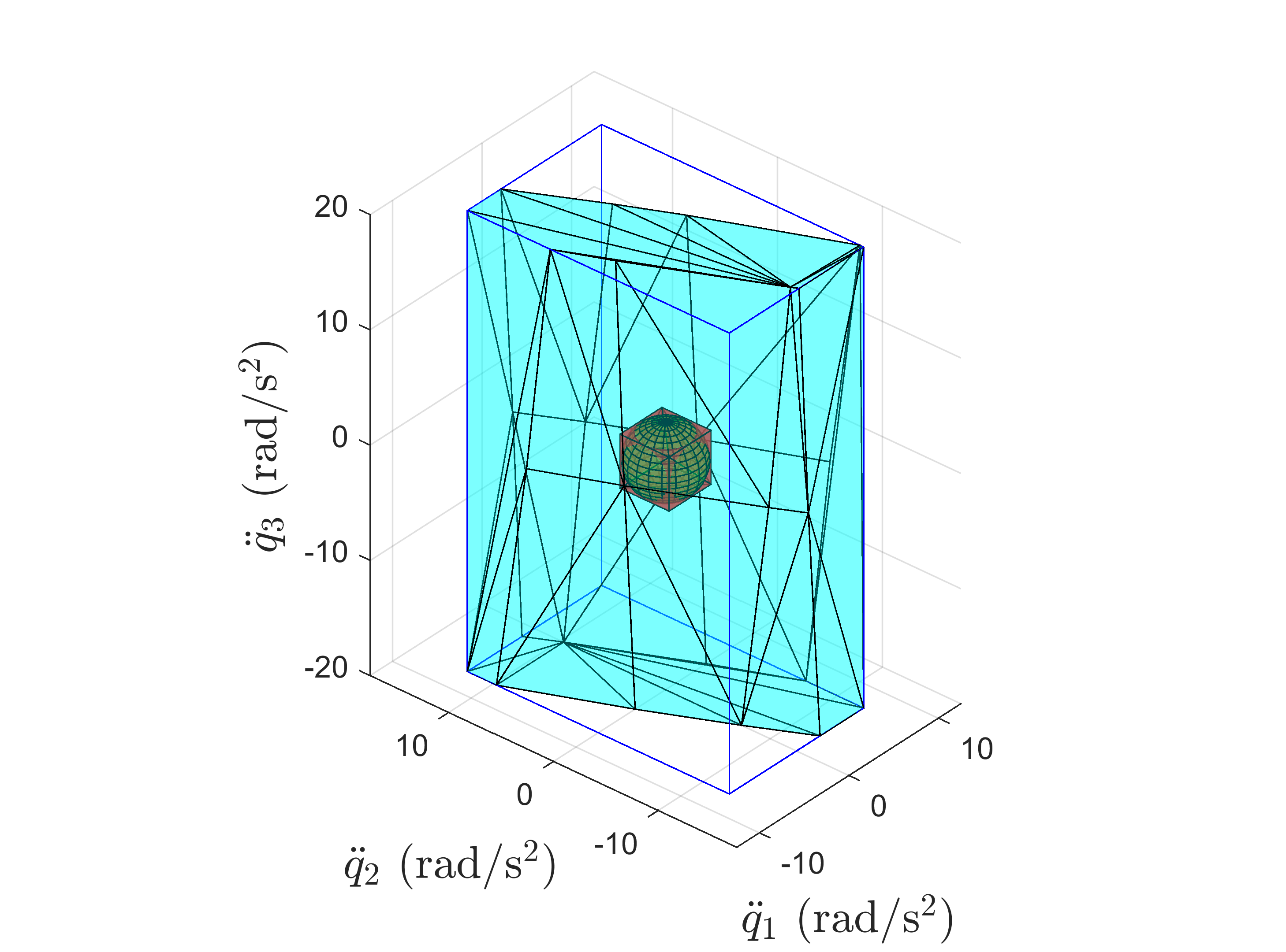
Figure 10: Future joint acceleration capability inner approximations during a prediction period $[t]$. For visibility, the polytope is bounded by the manufacturer’s limits $[\ddot{\operatorname{{\bf q}}}_{lim}]$.

VI Conclusion

Efficient set-based approaches for computing reliable inner approximations of a robot’s common capabilities over sets of joint states and with design parameter uncertainties are presented in this work. These approaches allow to not only consider the temporal evolution of the system over a small time horizon when computing the localized capabilities, but also allow to manage uncertainties to handle an imprecise/variable system describing a family of robotic manipulators.

The use of set-based approaches to evaluate capabilities provides many benefits over conventional approaches. One key benefit is the computation of certified inner approximations of the robot’s capabilities, allowing these approaches to be used in offline and online scenarios to improve the safety of robotic systems. The ability to automatically handle design parameter uncertainties and other system uncertainties affecting performance (e.g., inertial parameter errors [43]) allows for the use of simpler imprecise/variable models that accurately describe a complex system (e.g., modeling flexure-jointed mechanisms [18]). Also, the ability to consider sets of joint states allows to locally evaluate capabilities over a small time horizon, such that the robot’s performance in the near future can be better understood. The sets of joint states may also be used to analyze the capabilities along continuous trajectories via the use of branch-and-bound methods, as opposed to the standard sampling-based approach, allowing to properly understand worst-case conditions which can be used to improve the overall performance of the robot.

The low computation costs of many of the proposed inner approximations allow for real-time applications, enabling their use for rapid design analysis as well as their potential integration directly in to the robot controller. Therefore, a future application of this work may be the development of a certifiably safe robot controller which will use a properly formulated imprecise/variable system to safely estimate the robot’s true capabilities over a given time horizon. These capabilities may then be used directly in the controller to ensure that each controller action is achievable. Furthermore, by computing and incorporating the robot’s deceleration capabilities into the controller, it is be possible to enforce strict braking criteria to guarantee that collaborative systems are safe when in close proximity to a human.

Joshua K. Pickard received a B.Sc.E. degree in mechanical engineering with a mechatronics option in 2012, and a Ph.D. in mechanical engineering on uncertainty analysis and mechanism synthesis in 2018 from from the University of New Brunswick, Fredericton, New Brunswick, Canada. From 2018 to 2020 he was a postdoctoral fellow at Inria Bordeaux Sud-Ouest, Bordeaux, France, with the Auctus Team working on a modeling and analysis framework for imprecise and variable kinematic chains for the study of human motor-variabilities. Currently, he is a postdoctoral fellow at the University of New Brunswick working on research related to factories of the future and Industry 4.0.

Vincent Padois is a senior research scientist at Inria, centre Bordeaux Sud-Ouest in the Auctus team (Talence, France). From 2007 to 2020, he was an associate professor of Robotics at Sorbonne Université and ISIR (Paris, France). From 2006 to 2007 he was a postdoctoral researcher at the Stanford Artificial Intelligence Laboratory in the group of Prof. O. Khatib (Stanford, USA). He received his Ph.D. degree in Robotics and Automatic Control from INP de Toulouse in 2005. His main research interest is robot control in constrained contexts and dynamic environments, including wheeled mobile manipulators, humanoid robots and collaborative robots. Beyond control, his research activities in collaborative robotics are focused on virtual human models for the ergonomic quantification of the physical assistance of collaborative robots. He is also involved in research activities aiming at bridging the gap between adaptation and decision making techniques and model-based control through the use of machine learning and evolutionary algorithms.

Milan Hladík is an associate professor at the Department of Applied Mathematics of the Faculty of Mathematics and Physics, Charles University, Prague, Czech Republic. His research interests include interval computation, numerical analysis, optimization and operations research. He is a member of the editorial board of four international journals, including European Journal of Operational Research.

David Daney is a researcher at Inria Bordeaux Sud-Ouest, and leads the Project-Team Auctus, Inria-IMS (Univ. Bordeaux, Bordeaux INP, CNRS UMR 5218), Talence, France. He received the B. Eng in applied mathematics and computer science from University of Toulouse in 1996 and the M.Sc. and Ph.D. degrees in robotics from the University of Nice, Sophia Antipolis, France, in 1997 and 2000, respectively. He spent two years as a postdoctoral associate with C.M.W., France, to design a robotics system (2000) and with the LORIA Lab, Nancy, France, on computer arithmetic (2001). In 2002, he was an invited researcher with McGill University, Rutgers University, Laval University. From 2003 to 2013, he has been an Inria Research Scientist with the Inria Sophia Antipolis Research Center. His research interests are in the areas of parallel robotics, calibration, interval analysis, mechanical design, and assistive systems. Since 2013, he has been at the Inria research center in Bordeaux and in 2017 he founded the Auctus team in collaboration with the ENSC and the IMS. The aim of this team is to design collaborative robotic systems for man at work in industrial environments.

References

- [1] A. Ibanez, P. Bidaud, and V. Padois, Optimization-Based Control Approaches to Humanoid Balancing. Springer Netherlands, 2017, pp. 1–27.
- [2] S. Tonneau, A. Del Prete, J. Pettré, C. Park, D. Manocha, and N. Mansard, “An efficient acyclic contact planner for multiped robots,” IEEE Transactions on Robotics, vol. 34, no. 3, pp. 586–601, 2018.
- [3] C. Mastalli, R. Budhiraja, W. Merkt, G. Saurel, B. Hammoud, M. Naveau, J. Carpentier, L. Righetti, S. Vijayakumar, and N. Mansard, “Crocoddyl: An efficient and versatile framework for multi-contact optimal control,” in Proceedings of the IEEE RAS International Conference in Robotics and Automation, Paris, France, May 2020.
- [4] A. D. Prete, “Joint position and velocity bounds in discrete-time acceleration/torque control of robot manipulators,” IEEE Robotics and Automation Letters, vol. 3, no. 1, pp. 281–288, 2018.
- [5] S. Rubrecht, V. Padois, P. Bidaud, M. De Broissia, and M. D. S. Simoes, “Motion safety and constraints compatibility for multibody robots,” Autonomous Robots, vol. 32, no. 3, pp. 333–349, 2012.
- [6] W. Decre, R. Smits, H. Bruyninckx, and J. De Schutter, “Extending itasc to support inequality constraints and non-instantaneous task specification,” in 2009 IEEE International Conference on Robotics and Automation, 2009, pp. 964–971.
- [7] J. G. N. D. Carvalho Filho, E. A. N. Carvalho, L. Molina, and E. O. Freire, “The impact of parametric uncertainties on mobile robots velocities and pose estimation,” IEEE Access, vol. 7, pp. 69 070–69 086, 2019.
- [8] R. E. Moore, Interval analysis, ser. Prentice-Hall series in automatic computation. Englewood Cliffs, NJ: Prentice-Hall, 1966.
- [9] L. Jaulin, M. Kieffer, O. Didrit, and E. Walter, Applied Interval Analysis with Examples in Parameter and State Estimation, Robust Control and Robotics. Springer London, Aug. 2001.
- [10] R. E. Moore, R. B. Kearfott, and M. J. Cloud, Introduction to Interval Analysis. Philadelphia, PA: SIAM, 2009.
- [11] E. D. Popova and M. Hladík, “Outer enclosures to the parametric AE solution set,” Soft Comput., vol. 17, no. 8, pp. 1403–1414, 2013.
- [12] S. P. Shary, “Interval gauss-seidel method for generalized solution sets to interval linear systems,” Reliable Computing, vol. 7, no. 2, pp. 141–155, Apr 2001.
- [13] L. V. Kolev, “A method for outer interval solution of linear parametric systems,” Reliab. Comput., vol. 10, no. 3, pp. 227–239, 2004.
- [14] E. D. Popova and W. Krämer, “Inner and outer bounds for the solution set of parametric linear systems,” J. Comput. Appl. Math., vol. 199, no. 2, pp. 310–316, 2007.
- [15] A. Neumaier, “The wrapping effect, ellipsoid arithmetic, stability and confidence regions,” in Validation Numerics: Theory and Applications, R. Albrecht, G. Alefeld, and H. J. Stetter, Eds. Vienna: Springer, 1993, pp. 175–190.
- [16] N. Nedialkov, V. Kreinovich, and S. Starks, “Interval arithmetic, affine arithmetic, Taylor series methods: Why, what next?” Numerical Algorithms, vol. 37, pp. 325–336, 12 2004.
- [17] J.-P. Merlet, “Interval analysis for Certified Numerical Solution of Problems in Robotics,” International Journal of Applied Mathematics and Computer Science, 2009.
- [18] D. Oetomo, D. Daney, B. Shirinzadeh, and J.-P. Merlet, “An Interval-Based Method for Workspace Analysis of Planar Flexure-Jointed Mechanism,” Journal of Mechanical Design, vol. 131, no. 1, 12 2008.
- [19] M. Gouttefarde, D. Daney, and J.-P. Merlet, “Interval-analysis-based determination of the wrench-feasible workspace of parallel cable-driven robots,” IEEE Transactions on Robotics, vol. 27, no. 1, pp. 1–13, Feb 2011.
- [20] J. K. Pickard and J. A. Carretero, “An interval analysis method for wrench workspace determination of parallel manipulator architectures,” Transactions of the Canadian Society for Mechanical Engineering, vol. 40, no. 2, pp. 139–154, 2016.
- [21] J.-P. Merlet and D. Daney, “Appropriate design of parallel manipulators,” in Smart Devices and Machines for Advanced Manufacturing, L. Wang and J. Xi, Eds. London: Springer, 2008, pp. 1–25.
- [22] M. H. F. Kaloorazi, M. T. Masouleh, and S. Caro, “Collision-free workspace of parallel mechanisms based on an interval analysis approach,” Robotica, vol. 35, no. 8, p. 1747–1760, 2017.
- [23] J.-P. Merlet, “Interval analysis and robotics,” in Robotics Research, M. Kaneko and Y. Nakamura, Eds. Berlin, Heidelberg: Springer, 2011, pp. 147–156.
- [24] J.-P. Merlet and P. Donelan, “On the regularity of the inverse jacobian of parallel robots,” in Advances in Robot Kinematics, J. Lenarčič and B. Roth, Eds. Dordrecht: Springer Netherlands, 2006, pp. 41–48.
- [25] S. Bouchard, C. M. Gosselin, and B. Moore, “On the ability of a cable-driven robot to generate a prescribed set of wrenches,” ASME. J. Mechanisms Robotics, vol. 2, no. 1, 2009.
- [26] J. A. Carretero and C. M. Gosselin, “Wrench capabilities of cable-driven parallel mechanisms using wrench polytopes,” in Proceeding of the 2010 IFToMM Symposium on Mechanism Design for Robotics, Universidad Panamericana, Mexico City, Mexico, September 28–30 2010.
- [27] M. Gouttefarde and S. Krut, “Characterization of parallel manipulator available wrench set facets,” in Advances in Robot Kinematics: Motion in Man and Machine, J. Lenarčič and M. M. Stanisic, Eds. Dordrecht: Springer Netherlands, 2010, pp. 475–482.
- [28] S. P. Shary, “A new technique in systems analysis under interval uncertainty and ambiguity,” Reliable Computing, vol. 8, no. 5, pp. 321–418, Oct 2002.
- [29] G. M. Ziegler, Lectures on Polytopes, ser. Graduate Texts in Mathematics. Berlin: Springer, 1995, vol. 152.
- [30] R. E. Wendell and W. Chen, “Tolerance sensitivity analysis: Thirty years later,” Croatian Oper. Res. Rev., vol. 1, pp. 12–21, 2010.
- [31] M. Hladík, “Tolerance analysis in linear systems and linear programming,” Optim. Methods Softw., vol. 26, no. 3, pp. 381–396, 2011.
- [32] ——, “Weak and strong solvability of interval linear systems of equations and inequalities,” Linear Algebra Appl., vol. 438, no. 11, pp. 4156–4165, 2013.
- [33] J. Rohn, “Linear programming with inexact data is NP-hard,” ZAMM, Z. Angew. Math. Mech., vol. 78, no. Supplement 3, pp. S1051–S1052, 1998.
- [34] ——, “Solvability of systems of interval linear equations and inequalities,” in Linear Optimization Problems with Inexact Data, M. Fiedler et al., Ed. Boston, MA: Springer, 2006, ch. 2, pp. 35–77.
- [35] S. P. Shary, “Solving the linear interval tolerance problem,” Mathematics and Computers in Simulation, vol. 39, no. 1, pp. 53 – 85, 1995.
- [36] E. D. Popova, “Inner estimation of the parametric tolerable solution set,” Comput. Math. Appl., vol. 66, no. 9, pp. 1655–1665, 2013.
- [37] J. Rohn, “Inner solutions of linear interval systems,” in Proceedings of the International Symposium on Interval Mathematics on Interval Mathematics 1985. Berlin, Heidelberg: Springer, 1986, pp. 157–158.
- [38] P. Chiacchio, Y. Bouffard-Vercelli, and F. Pierrot, “Evaluation of force capabilities for redundant manipulators,” in Proceedings of IEEE International Conference on Robotics and Automation, vol. 4, April 1996, pp. 3520–3525.
- [39] A. Skuric, V. Padois, and D. Daney, “On-line force capability evaluation based on efficient polytope vertex search,” 2020.
- [40] J. K. Pickard, “Software: Inner Approximation Algorithms for Interval Linear Systems of Equations,” June 2020. [Online]. Available: https://figshare.com/articles/Software_Inner_Approximation_Algorithms_for_Interval_Linear_Systems_of_Equations/12472748
- [41] J. K. Pickard, J. A. Carretero, and J.-P. Merlet, “Appropriate analysis of the four-bar linkage,” Mechanism and Machine Theory, vol. 139, pp. 237 – 250, 2019.
- [42] L. Jaulin, “Path planning using intervals and graphs,” Reliable Computing, vol. 7, pp. 1–15, 02 2001.
- [43] N. Giftsun, A. Del Prete, and F. Lamiraux, “Robustness to Inertial Parameter Errors for Legged Robots Balancing on Level Ground,” in International Conference on Informatics in Control, Automation and Robotics (ICINCO 2017), Madrid, Spain, Jul. 2017.