LinDA: linear models for differential abundance analysis of microbiome compositional data

Huijuan Zhou (zhouhuijuan@mail.shufe.edu.cn) Shanghai University of Finance and Economics Texas A&M University Renmin University of China Kejun He (kejunhe@ruc.edu.cn) Renmin University of China Jun Chen (chen.jun2@mayo.edu) Mayo Clinic Corresponding author Xianyang Zhang (zhangxiany@stat.tamu.edu) Texas A&M University Corresponding author
Abstract

Differential abundance analysis is at the core of statistical analysis of microbiome data. The compositional nature of microbiome sequencing data makes false positive control challenging. Here, we show that the compositional effects can be addressed by a simple, yet highly flexible and scalable, approach. The proposed method, LinDA, only requires fitting linear regression models on the centered log-ratio transformed data, and correcting the bias due to compositional effects. We show that LinDA enjoys asymptotic FDR control and can be extended to mixed-effect models for correlated microbiome data. Using simulations and real examples, we demonstrate the effectiveness of LinDA.


Keywords: Compositional effect, Differential abundance analysis, False discovery rate, Multiple testing.

1 Background

The role of the human microbiome in health and disease has been intensively studied over the past few years, see, e.g., [1, 2], for several reviews. Potentially pathogenic or probiotic microorganisms can be identified by analyzing their abundances in a microbial ecosystem (e.g., the human gut) with respect to some covariate of interest such as disease status. Current prevailing technologies for studying the human microbiome use metagenomic sequencing, where either the DNA of a taxonomically informative gene (e.g. 16S rRNA) or all the genomic DNA in the microbial genome is sequenced. After obtaining the raw sequencing reads, the reads can be clustered into operational taxonomic units (OTUs), denoised into amplicon sequence variants (ASVs), or mapped to a microbial reference database (taxa) using existing bioinformatics pipelines such as UPARSE, DADA2, and MetaPhlAn [3, 4, 5]. For simplicity, we use the term taxon (pl. taxa) to represent any taxonomic unit (OTU/ASV/taxon) from a bioinformatics pipeline. Therefore, after bioinformatics processing, we have an abundance table recording the frequencies of detected taxa in the samples, together with a meta data table capturing the sample-level information. Differential abundance analysis is then carried out based on the abundance and meta data table.

Ideally, we want to measure the absolute abundance of the microorganisms, i.e., the number of microorganisms per unit area/volume at the microbial ecosystem, and differential abundance analysis is performed on the absolute abundance data. However, the data from a sequencing experiment only captures the relative abundance (compositional) information since the total sequence read count, also known as sequencing depth or library size, does not reflect the total microbial load in the specimen due to the complex chemistry involved in sequencing [6, 7]. Although there are several experimental techniques such as qPCR, spike-in and flow cytometry that can be used to achieve absolute abundance measurement, the severe limitations of these techniques prevent their wide adoption [8]. Therefore, the prevailing sequencing protocol is still only able to measure the relative abundances. Drawing inferences about the changes on the unknown absolute abundance based on the measured relative abundance data is challenging due to missing the total microbial load information. The increase or decrease in the abundance of some taxa with respect to a covariate of interest automatically results in changes in the relative abundances of all other taxa, a statistical phenomenon known as compositional effects. Therefore, using the standard statistical techniques such as two-sample t-test, Wilcoxon rank sum test, and linear regression analysis ignoring the compositional nature of the data could lead to a large number of false discoveries.

For the differential abundance problem to be well defined, one has to make assumptions. One major assumption is that the differential signal is sparse, i.e., only a small proportion of taxa are associated with the covariate of interest. Although many studies have supported the sparse signal assumption, there are also studies support dense signal hypotheses, where a large number of taxa are differential with small effect sizes [9, 10]. Therefore, the validity of a method and the definition of true or false positive depends on the specific assumption one is willing to accept. Here our goal is to provide a statistical tool that could be potentially useful for pinpointing top candidate taxa for further biological validation.

To address compositional effects in differential analysis, one popular approach is robust normalization. It involves calculating a normalizing factor (scale factor), which is robust to a small number of differential taxa and could well capture the sequencing effort for the non-differential part. Therefore, dividing by such a normalizing factor will bring the abundance of the non-differential taxa to the same scale while retaining the differences for those differential ones. Assuming the number of differential taxa is small, different strategies have been used to calculate a robust normalizing factor including TMM, RLE, CSS, and GMPR [11, 12, 13, 14]. We list these methods in Additional file Supplementary material: Table S1. In contrast, the naive total sum scaling (TSS) normalization, which divides the counts by the library size, is not a robust normalization method [14].

These normalization techniques can be combined with different statistical procedures in differential abundance analysis. For example, we can divide the counts by the normalizing factor from the normalization techniques in Additional file Supplementary material: Table S1 and then apply standard statistical tools based on the normalized data. The normalizing factor could also be included as an offset in regression models such as edgeR [15], DESeq2 [16], MicrobiomeDDA [17], and metagenomeSeq [13], where the TMM, RLE, GMPR, and CSS normalization are the accompanying normalization methods. The recently developed MaAsLin2 [18] uses log linear models on the normalized abundance data. Different normalization approaches including TSS, TMM, CSS, and CLR are options in MaAsLin2. A variant to the robust normalization approach is to find a reference taxon or a set of reference taxa, which are assumed to be non-differential with respect to the covariate of interest. The data are then normalized by the count of the reference taxon (or the sum of the counts of the reference taxa). This strategy was used in RAIDA [19] and DACOMP [20].

Another line of methods to tackle the compositional effect uses (log) ratio approach since only ratios are well defined for compositional data [21]. The ALDEx2 method by [22] uses the centered log-ratio (CLR) transformation, where the counts of a sample are divided by their geometric mean before taking logarithms. Differential abundance analysis is then performed using Wilcoxon rank sum test or t-test based on the CLR transformed data. In the CLR approach, the geometric mean can also be regarded as a robust normalizing factor. The ANCOM proposed by [23] computes the pairwise ratios of the relative abundances and identifies the taxa with the most differential ratios. This is based on the observation that the abundance ratios for those differential taxa to other taxa are all differential assuming distinct effect sizes while the ratios for those non-differential taxa are mostly non-differential. Therefore, by analyzing the pattern of the pairwise ratios, one could distinguish the differential taxa from a background of non-differential taxa with high accuracy. Recently, a bias-corrected version of ANCOM (called ANCOM-BC) has been proposed [24], which uses a linear regression framework based on log-transformed taxa count and estimates the unknown bias term due to the compositional effect through an EM algorithm.

In the work of [25, 26], the authors evaluated several popular methods in differential abundance analysis (ANCOM-BC/MaAsLin2 not included) and showed that the inflation of the false discovery rate (FDR) is still a ubiquitous problem, and no method is satisfactory in all aspects. A method that is computationally efficient, relatively robust and powerful, and flexible enough to allow covariate adjustment and application to correlated microbiome data is still lacking in the field. In this paper, we propose a linear regression framework for differential abundance analysis (LinDA) to fill the methodological gap. LinDA involves three simple steps that can be carried out efficiently. First, it runs linear regressions using the CLR transformed abundance data as the response. Then it identifies a bias term due to the compositional effect and corrects for the bias using the mode of the regression coefficients across different taxa. Finally, it computes the p-values based on the bias-corrected regression coefficients and applies the Benjamini-Hochberg (BH) procedure to control the FDR. We rigorously prove the asymptotic FDR control of the proposed method, making it the first procedure that enjoys a theoretical FDR control guarantee. Our approach is related to ANCOM-BC but differs in several aspects. (i) Our derivation provides a clear interpretation of the bias term and suggests a simple way to correct it. (ii) Our procedure does not involve the EM-algorithm and can be 100–1000 times faster than ANCOM-BC in our numerical studies. (iii) Our method can be directly extended to the mixed-effect models. Longitudinal and repeated measurement-based microbiome studies have been increasingly common [27, 28] but statistical tools for correlated microbiome data analysis remain scarce. LinDA can analyze the correlated microbiome data using the classic linear mixed effects models. Through extensive simulation studies and real data analyses, we show that the new method outperforms the state-of-the-art approaches in terms of FDR control and power.

2 Results

2.1 Numerical studies

Setups We conducted comprehensive simulations to evaluate the performance of the proposed method under different setups. We set m=500π‘š500m=500 as the baseline for the number of taxa, which is similar to the number of tests at the species level for a typical microbiome study. We investigated the sample size n=50, 200𝑛50200n=50,\;200 representing small and large sample sizes, respectively. More combinations of mπ‘šm and n𝑛n were studied in additional settings. We generated the absolute abundances from the log normal distribution and considered three cases for the covariate of interest and confounders: the covariate of interest follows the Bernoulli distribution and no confounder (denoted as C0), the covariate of interest follows the standard normal distribution and no confounder (C1), and the covariate of interest follows the Bernoulli distribution and two confounders (C2). In addition to the basic setting (log normal abundance distribution, denoted as S0), we investigated other settings to study the robustness of the proposed method including zero-inflated absolute abundances (S1), correlated absolute abundances (S2), gamma abundance distribution (S3), smaller mπ‘šm (S4), smaller n𝑛n (S5), 10-fold difference in library size (S6), negative binomial abundance distribution (S7) and correlated microbiome data generated by mixed-effect model (S8). See section 5.6 for more details.


Competing methods We compared our method with ANCOM-BC, ALDEx2, DESeq2, edgeR, metagenomeSeq and MaAsLin2. For DESeq2 and edgeR, we replaced their native normalization methods with GMPR normalization, which was shown to improve the power and false positive control in differential abundance analysis [14]. For metagenomeSeq, there are two implementations, fitZig and fitFeatureModel, in the R Bioconductor package metagenomeSeq. Currently, fitFeatureModel is only applicable to binary covariate case (C0). We use metagenomeSeq2 and metagenomeSeq to denote the fitFeatureModel and fitZig procedures, respectively. We also compared with the standard non-parametric methods: Wilcoxon rank sum test for case C0 (a binary covariate) and Spearman correlation test for case C1 (a continuous covariate), both with the GMPR normalized data.

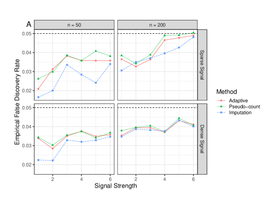
For the proposed method, we considered two zero-handling approaches. The first approach adds a pseudo count of 0.5 to all the counts, which is widely used in microbiome data analysis on the log scale. However, it has been shown to be problematic under certain situations [20]. We thus designed a new imputation-based approach, where the zeros were imputed by Ns/(maxk:Yi​k=0⁑Nk)subscript𝑁𝑠subscript:π‘˜subscriptπ‘Œπ‘–π‘˜0subscriptπ‘π‘˜N_{s}/(\max_{k:Y_{ik}=0}N_{k}) for i𝑖ith taxon in s𝑠sth sample, where Nssubscript𝑁𝑠N_{s} denotes the library size (sequencing depth) of s𝑠sth sample and Yi​ksubscriptπ‘Œπ‘–π‘˜Y_{ik} denotes the read count of i𝑖ith taxon in kπ‘˜kth sample. In other words, zeros were imputed differently according to the library size of the sample, and zeros in the sample with a larger library size were replaced with larger fractions. In this imputation approach, we treat zeros as left-censored missing data. Suppose we only know the library sizes, then a natural strategy is to impute zeros in proportion to the library size with the sample of the largest library size receiving a fractional count close to 1 (in our approach, we simply set it as 1). The purpose of the imputation strategy is to reduce false positives when the library size is correlated with the covariate of interest. As shown in the simulation studies, the pseudo-count approach worked sufficiently well in most settings except the setting S6, where the library size between the groups differed by 10 folds. In contrast, the imputation approach reduced the false positive rate extensively for the setting S6 (Additional file Supplementary material: Fig. S1). However, it was slightly less powerful than the pseudo-count approach when the library size was a not confounder (Additional file Supplementary material: Fig. S2). Thus, in the implementation, we used an adaptive approach: we first tested the association between the covariate of interest and the library size. If the p-value was smaller than 0.1, we used the imputation approach conservatively; otherwise, we used the pseudo-count approach. Additional file Supplementary material: Fig. S1 and S2 show that the adaptive method controls the false positives when the library sizes are very different among groups while retaining the power when the library sizes are similar.

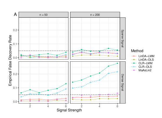
The proposed LinDA method can be viewed as a three-step procedure: CLR-OLS-BC (OLS stands for ordinary least squares and BC stands for bias correction), which can be easily extended to the linear mixed-effects model using CLR-LMM-BC (LMM stands for linear mixed-effect model). In the setting S8 (correlated microbiome data), we compared CLR-LMM-BC to CLR-OLS-BC, CLR-OLS, and CLR-LMM to demonstrate the utility of LinDA for correlated microbiome data analysis.


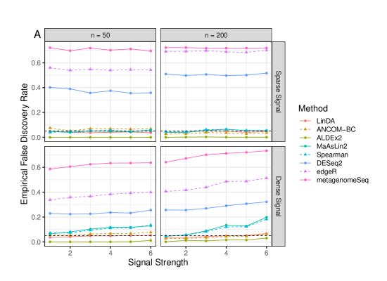
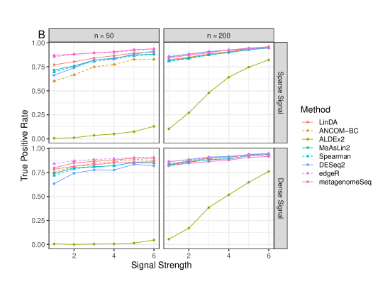
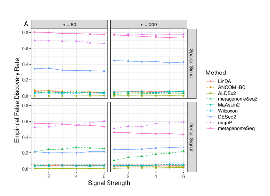
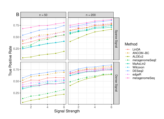
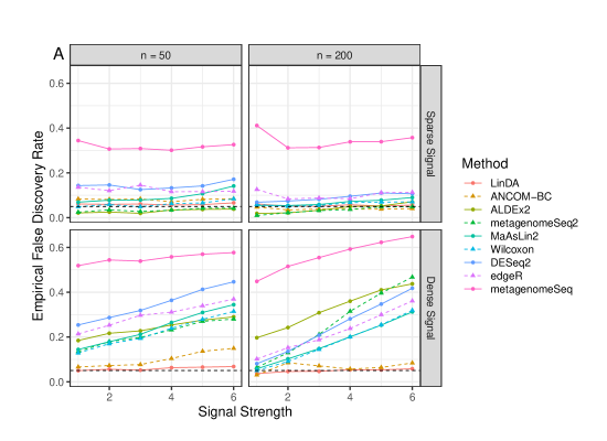
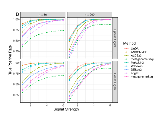
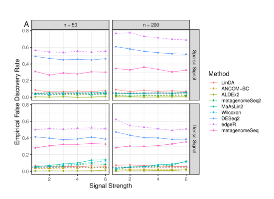
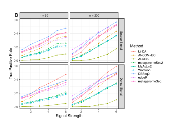
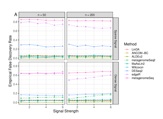
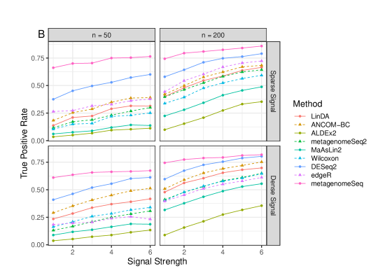
Results We use S0C0 (log normal abundance distribution, a binary covariate) to denote the setting S0 (log normal abundance distribution) with the covariate design C0 (a binary covariate) and likewise for other setups. For S0, we studied all the three covariate designs (C0–C2), and for S1–S8, we only performed C0 for demonstration. We found that DESeq2, edgeR and metagenomeSeq had severe FDR inflation under most settings. To increase the readability of the results (presented in figures), we did not include them in the main comparison and focused on the comparison between LinDA, ANCOM-BC, ALDEx2, metagenomeSeq2, MaAsLin2 and Wilcoxon (Fig. 1–2 and Additional file Supplementary material: Fig. S1–S15). Full results of all methods are presented in Additional file Supplementary material: Fig. S20–S30.

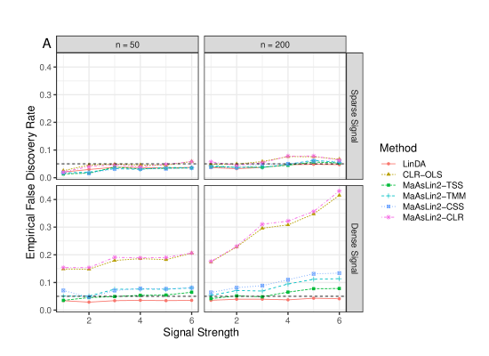
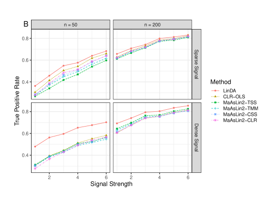
We first point out that MaAsLin2 with CLR normalization is essentially the same as the CLR-OLS procedure we described earlier. Additional file Supplementary material: Fig. S3 compares LinDA, CLR-OLS, MaAsLin2-TSS, MaAsLin2-TMM, MaAsLin2-CSS and MaAsLin2-CLR under the setting S0C0 (log normal abundance distribution, a binary covariate). We can see that MaAsLin2-CLR is close to CLR-OLS, both of which suffer from FDR inflation. We included MaAsLin2 with its default configuration (i.e., TSS normalization) in our comparisons below.

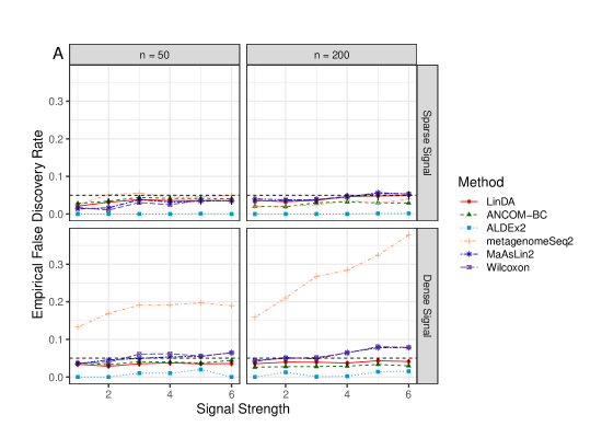
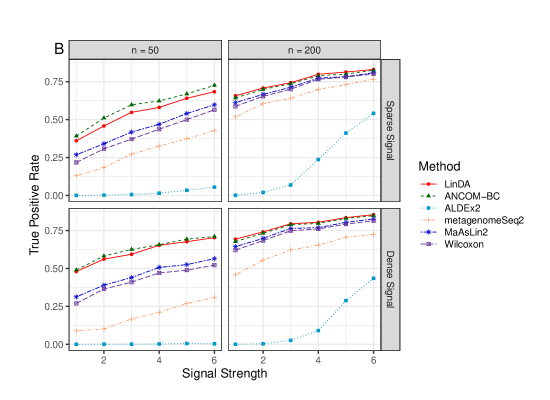
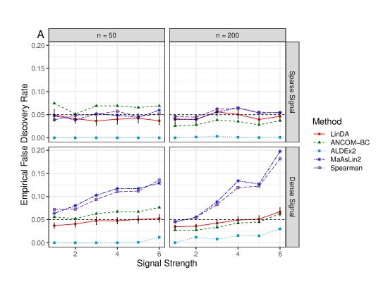
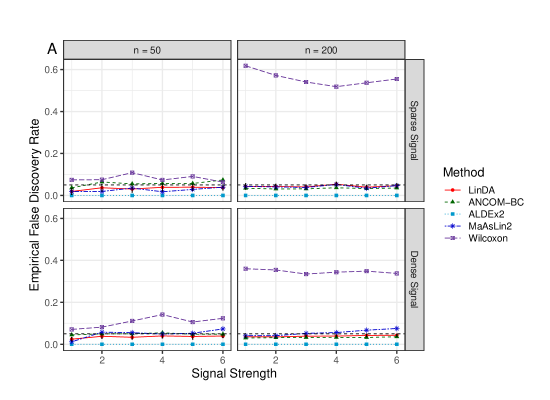
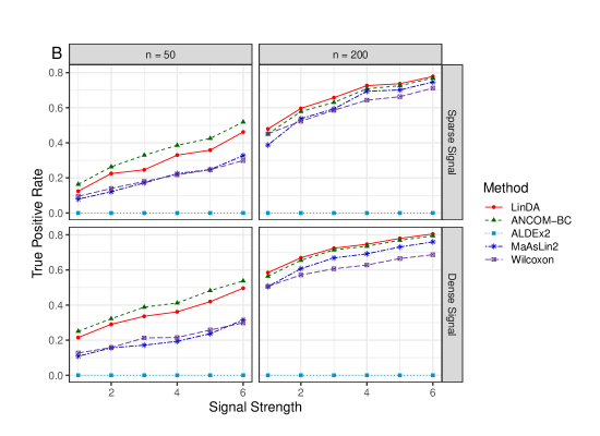
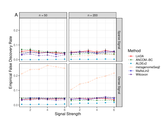
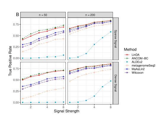
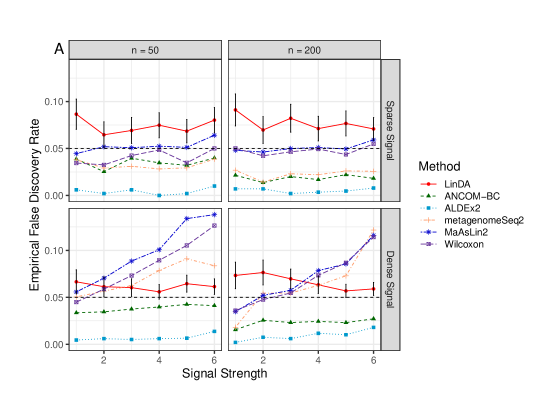
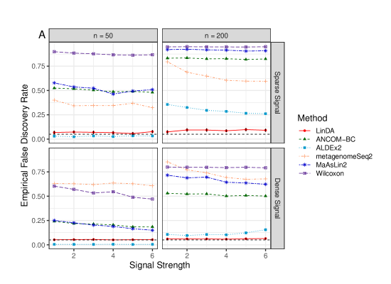
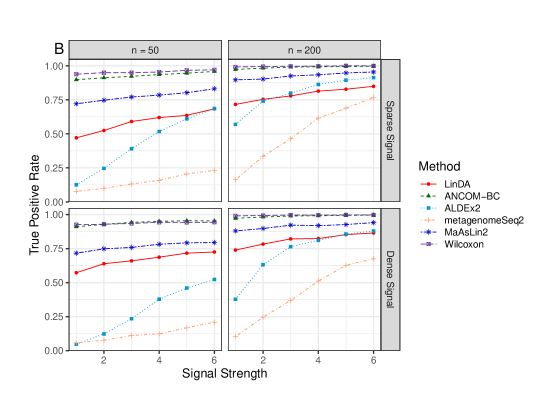
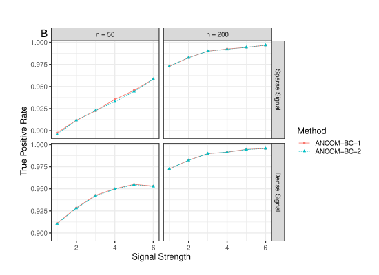
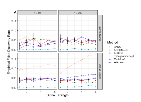
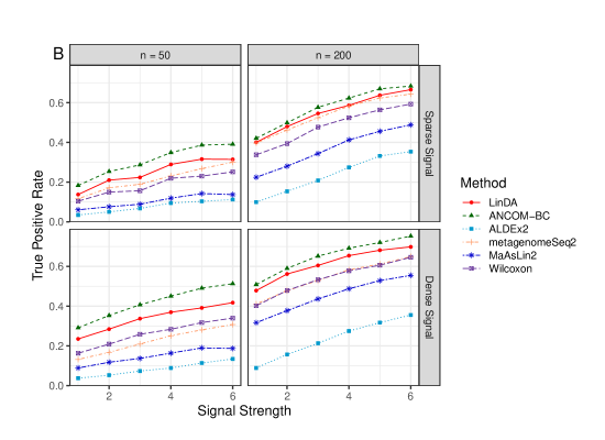
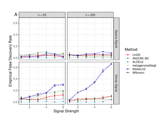
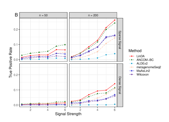
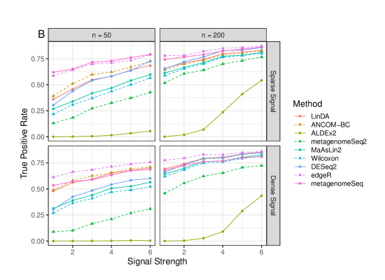
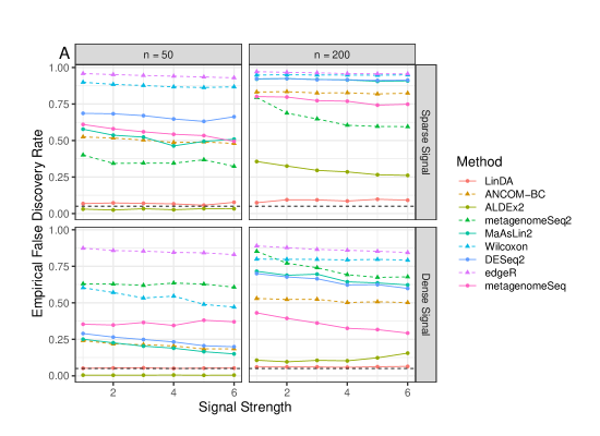
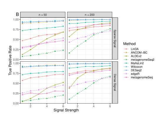
Fig. 1 and Additional file Supplementary material: Fig. S4 and S5 show the results of the competing methods under the log-normal abundance distribution with three covariate designs: a binary covariate (S0C0), a continuous covariate (S0C1), and a binary variable of interest with confounders (S0C2), respectively. Generally speaking, LinDA and ANCOM-BC have the best FDR and power trade-off. Under C0 and C2 (Fig. 1 and Additional file Supplementary material: Fig. S5), both methods control the FDR around the target level, and ANCOM-BC is slightly more powerful than LinDA when the sample size is small. However, under C1 (Additional file Supplementary material: Fig. S4), LinDA controls FDR at the target level at both sample sizes while ANCOM-BC has slight FDR inflation when the sample size is small. LinDA is also slightly more powerful than ANCOM-BC at a small sample size. The Wilcoxon rank sum test based on GMPR normalized data and MaAsLin2 perform well under C0 (a binary covariate, Fig. 1) with slightly inflated FDR at larger effect sizes and reasonable power across settings. In contrast, for a continuous covariate (C1, Additional file Supplementary material: Fig. S4), the Spearman rank correlation test and MaAsLin2 have large FDR inflation when the signal is dense. When there are confounders (C2, Additional file Supplementary material: Fig. S5), Wilcoxon has severe FDR inflation when the sample size is large due to its inability to adjust for confounders, while MaAsLin2 provides acceptable results as under C0. ALDEx2 is a conservative method, which offers the strongest FDR control but is much less powerful. metagenomeSeq2 performs well when the signal is sparse but fails to control the FDR when the signal is dense. We also studied the effect of zero inflation and the correlations among taxa (S1C0 and S2C0, Additional file Supplementary material: Fig. S6 and S7), where we observed similar patterns such that LinDA and ANCOM-BC had overall the best performance among the compared methods.

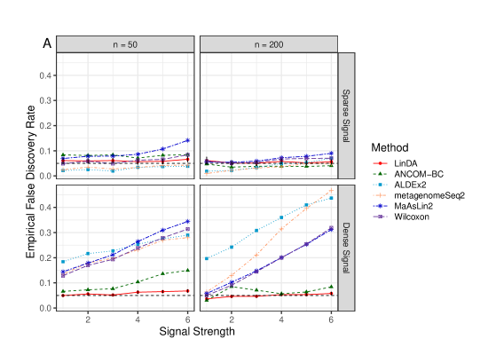
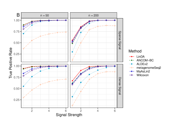
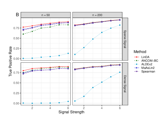
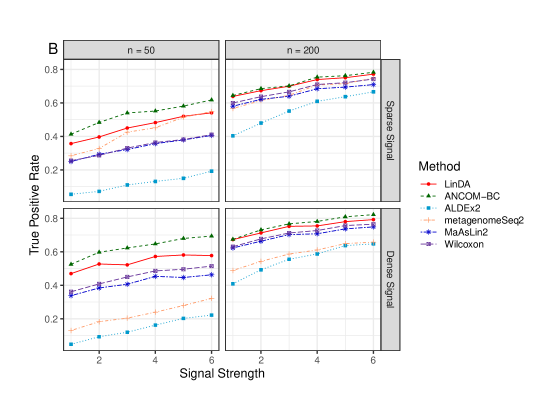
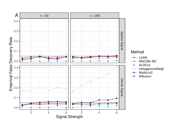
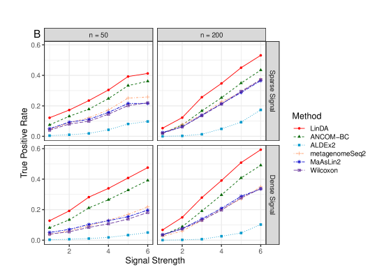
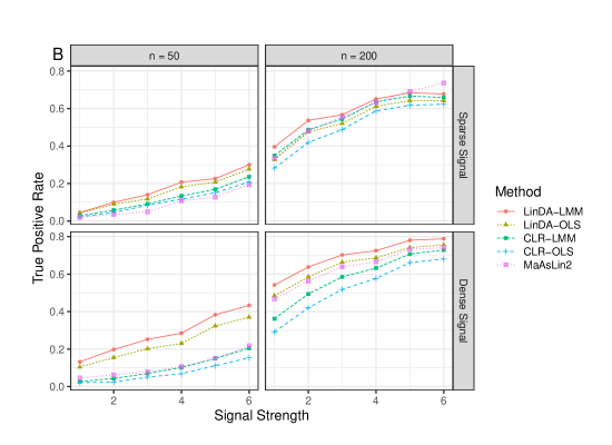
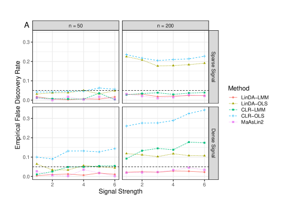
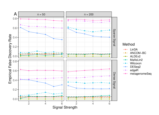
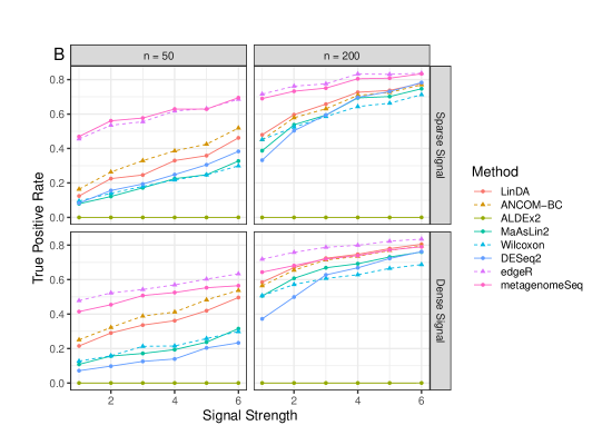
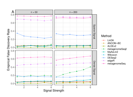
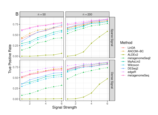
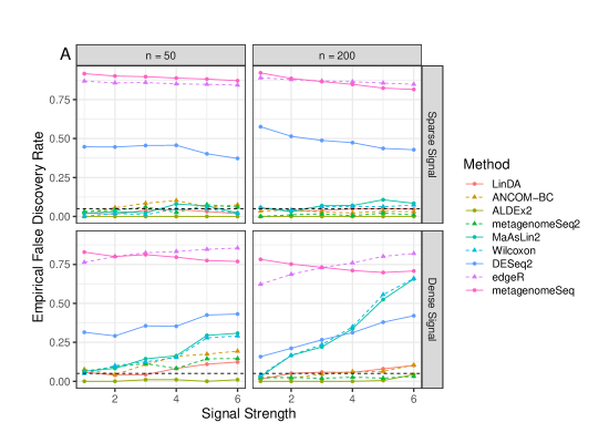
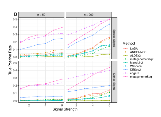
Since LinDA assumes a log normal distribution of the absolute abundance, it is interesting to evaluate its performance when the log normal assumption is violated. We thus simulated the absolute abundance data using a gamma distribution (S3C0), and the results are depicted in Fig. 2. It shows that LinDA controls the FDR close to the target level and has the highest power. When the signal is dense (20%), ANCOM-BC has a noticeable FDR inflation while ALDEx2, metagenomeSeq2, MaAsLin2 and Wilcoxon have severe FDR inflation when the signal is dense.

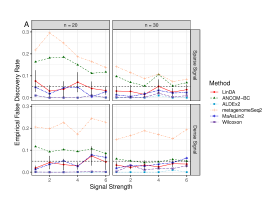
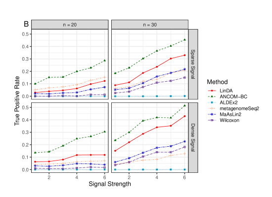
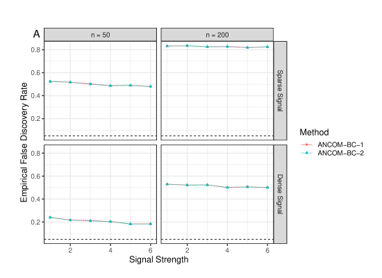
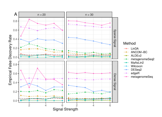
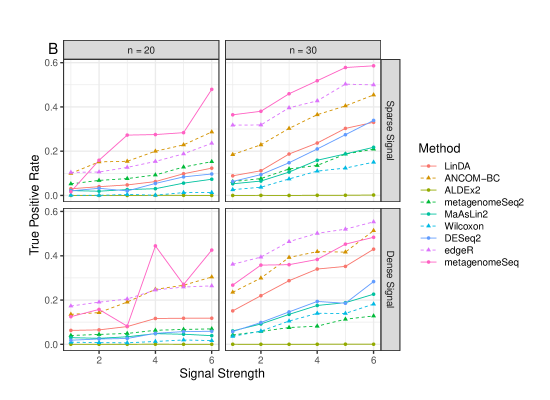
With a smaller number of taxa (m=50π‘š50m=50, S4C0, Additional file Supplementary material: Fig. S8), ANCOM-BC controls the FDR and the power is also high. LinDA is the most powerful but it has slight FDR inflation. metagenomeSeq2, MaAsLin2 and Wilcoxon control the FDR but are less powerful in the case of sparse signal. However, when the signal is dense, they could not control the FDR properly. When the sample size is very small (n=20𝑛20n=20 or 30, S5C0), LinDA controls the FDR around the target level and maintains high power (Additional file Supplementary material: Fig. S9). ANCOM-BC and metagenomeSeq2 have large FDR inflation and the inflation seems to increase as the sample size gets smaller. MaAsLin2 and Wilcoxon are much less powerful and ALDEx2 has virtually no power. Under the setting S6C0, where the sequencing depth differs by 10 folds, only ALDEx2 and our proposed method with adaptive zero-handling approach are able to control the FDR (Additional file Supplementary material: Fig. S10). LinDA achieves a better performance in both the FDR control and power than ALDEx2. It is interesting that ALDEx2 performs better under S6C0 than under other settings. We point out here that when we implemented ANCOM-BC, we disabled its zero treatment. To further investigate whether its zero treatment option improves its performance, we also run the procedure enabling its zero treatment (zero_cut = 0.9, lib_cut = 1000, struc_zero = TRUE), and found the results were very similar (S6C0, Additional file Supplementary material: Fig. S11).

Under the previous simulation settings, we found that DESeq2 and edgeR had the worst false positive control (Additional file Supplementary material: Fig. S20–S28). As the two methods assume negative binomial distribution for the counts, it is interesting to see their performance when the data are generated by their assumed model (S7C0). Additional file Supplementary material: Fig. S29 shows that DESeq2 and edgeR (and metagenomeSeq) remain to have serious FDR inflation, indicating that the normalization approach to address the compositional effect is not sufficient. In contrast, LinDA and ANCOM-BC perform the best among competitors as in other settings, and ANCOM-BC achieves higher power than LinDA (Additional file Supplementary material: Fig. S12).

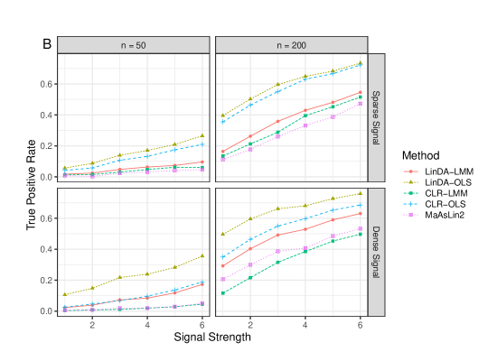
Finally, we applied LinDA to correlated microbiome data (S8C0), where the other competing methods except MaAsLin2 are not applicable to correlated samples. Additional file Supplementary material: Fig. S13 and S14 compare the methods CLR-LMM-BC (LinDA-LMM), CLR-OLS-BC (LinDA-OLS), CLR-LMM, CLR-OLS and MaAsLin2 for correlated data. In the scenario of comparing the pre-treatment and post-treatment samples (S8.1, Additional file Supplementary material: Fig. S13), we could clearly see that ignoring the bias tremendously increases the FDR level especially under dense signals (LinDA-LMM vs CLR-LMM). In addition, LinDA-LMM is more powerful than LinDA-OLS due to its ability to exploit the correlation between pre- and post-treatment samples. Under the replicate sampling setting (S8.2, Additional file Supplementary material: Fig. S14), we see that the LinDA-OLS has significant FDR inflation by treating the replicate samples as independent ones. In contrast, LinDA-LMM controls the FDR at the target level. MaAsLin2 control the FDR under both settings but is less powerful than LinDA-LMM.

Based on the presented simulation settings, we summarize that LinDA and ANCOM-BC have overall the most robust performance among the methods evaluated. However, ANCOM-BC is computationally intensive. As shown in Table 1, LinDA could be 100–1000 times faster than ANCOM-BC, making LinDA a highly scalable method in practice. In addition, the extension of LinDA to the mixed-effect models is easily carried out and performs well.

2.2 Real data applications

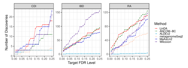
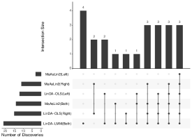
Datasets We applied LinDA and the competing methods to three real datasets with independent samples from the studies of C. difficile infection [CDI, 29], inflammatory bowel disease [IBD, 30], and rheumatoid arthritis [RA, 31]. To demonstrate the use of LinDA on correlated microbiome samples, we applied LinDA to a dataset from the study of the smoking effect on the human upper respiratory tract [SMOKE, 32]. We used the microbiome samples from the throat for illustration, where each subject has two samples from the left and right sides of the throat. The CDI and RA datasets were provided by the authors while the IBD and the SMOKE datasets were downloaded from the Qiita database [33] with the study ID 1460 and 524. All the datasets have binary phenotypes. Antibiotics use is the confounder for the IBD dataset (p=0.03𝑝0.03p=0.03 and OR = 0) while sex is the confounder for the SMOKE dataset (p=0.02𝑝0.02p=0.02 and OR= 2.26). They will be adjusted in methods that are capable of covariate adjustment. We excluded samples with less than 1000 read counts and taxa which appear in less than 10% of the samples. The basic characteristics for the four filtered datasets are summarized in Table 2. We compared the detection power as well as their overlap patterns for LinDA, ANCOM-BC, ALDEx2, metagenomeSeq2, MaAsLin2 and Wilcoxon. Specifically, we compared the number of discoveries at different FDR levels (0.01–0.25) and used UpSet plot [34] to show the overlap at the target FDR of 0.1. We used winsorization at quantile 0.97 to reduce the impact of potential outliers as recommended in [17].


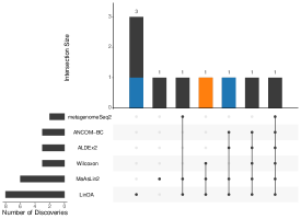
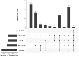
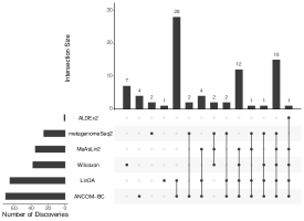
Results For the CDI dataset, LinDA or MaAsLin2 made the most discoveries at different FDR levels (Fig. 3). At 10% FDR, LinDA discovered eight and MaAsLin2 discovered six taxa associated with CDI. In contrast, ANCOM-BC, ALDEx2, and Wilcoxon discovered three while metagenomeSeq2 discovered two. As discussed in [29], subjects with CDI were more likely to have the bacterial family Lachnospiraceae and Erysipelotrichaceae. LinDA found one more taxon belonging to Lachnospiraceae than other methods (blue bars in Fig. 4). Besides, LinDA, MaAsLin2 and Wilcoxon found one differential taxon belonging to Erysipelotrichaceae while the other three methods did not identify any (orange bar in Fig. 4). For the IBD dataset, LinDA detected a similar number of taxa as ANCOM-BC and MaAsLin2. Wilcoxon rank sum test detected a large number of taxa associated with the disease status, but this could be due to the confounding effects of antibiotics use since it could not adjust for covariates. From Fig. 4, we observe that most discoveries by LinDA are shared by ANCOM-BC, MaAsLin2 or Wilcoxon. For the RA dataset, LinDA detected a similar number of taxa as ANCOM-BC and more taxa than other methods. The differential taxa detected by LinDA and ANCOM-BC largely overlapped. Overall, the results are consistent with the simulation studies.

Finally, we applied LinDA-LMM and MaAsLin2 to the SMOKE dataset, where each subject has two replicate samples from the throat. The aim is to identify smoking-associated taxa adjusting for the sex. To account for the correlation between the replicate samples, we included a subject-level random intercept in LinDA-LMM. As a comparison, we also applied LinDA-OLS and MaAsLin2 to the right and left throat samples separately. LinDA-OLS based on the left or right throat samples alone discovered 12 and 15 differential taxa at 10% FDR. When both left and right samples were used in LinDA-LMM, 21 differential taxa were identified, covering the majority of the taxa identified based on the left or right throat samples alone (Fig. 4). In addition, LinDA-LMM detected five taxa that were missed by analyzing the left or right samples separately. Compared to MaAsLin2, LinDA-LMM discovered seven more differential taxa. Therefore, LinDA-LMM provides a convenient way to analyze correlated microbiome datasets and enjoys the power improvement by analyzing all samples together.

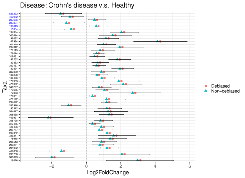
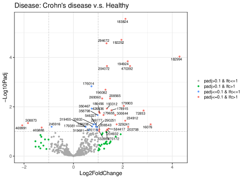
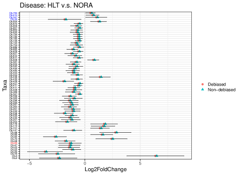
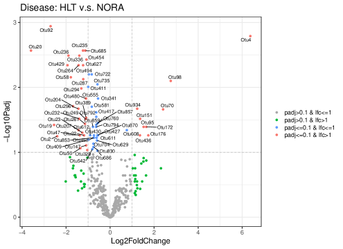
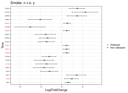
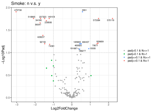
To visualize the results, LinDA provides a function to generate the effect size plot and volcano plot for differential taxa. Additional file Supplementary material: Fig. S16–S19 display the effect size plots of differential taxa at FDR level of 0.1 and volcano plots for the four datasets, respectively. In the effect size plots (Additional file Supplementary material: Fig. S16A–S19A), the taxa in black are detected by LinDA and taxa in red are detected solely by LinDA. In Additional file Supplementary material: Fig. S16A (CDI), the taxa in blue are missed by LinDA but detected by one or more other methods. In Additional file Supplementary material: Fig. S17A (IBD) and S18A (RA), the taxa in blue are missed by LinDA but detected by two or more other methods. No taxa are detected by MaAsLin2 but missed by LinDA-LMM for the SMOKE dataset. Based on the effect size plots for the CDI, IBD and RA datasets, we can see that, for the taxa solely detected by LinDA, the effect sizes tend to be underestimated without bias correction and bias correction improves the power in these cases. On the contrary, for the taxa missed by LinDA, the effect sizes tend to be overestimated without bias correction. In addition, we observe that the differential taxa for the IBD, CDI and RA datasets are more unbalanced (i.e., more negative or positive associations) while the differential taxa for the SMOKE dataset are relatively balanced (i.e., similar numbers of negative and positive associations). Indeed, the effect size plots, where we plot both the debiased and un-debiased coefficients, revealed larger biases for the IBD, CDI, and RA datasets.

3 Discussion

Differential abundance analysis is at the core of the statistical analysis of microbiome data. Microbiome data are compositional in nature and all we know are the relative abundances, making the identification of differentially abundant taxa at the ecological site particularly challenging [6, 7]. Numerous differential abundance analysis methods have been proposed focusing on addressing the compositional effects [15, 16, 17, 13, 19, 20, 22, 23, 24]. Among all the competing methods, ANCOM-BC is the state-of-the-art method, it has been demonstrated to be more robust and powerful than the competing methods. However, there are two drawbacks of ANCOM-BC. First, it is computationally intensive for large-scale microbiome datasets such as the AmericanGut dataset. Due to the huge inter-subject variation, large-scale microbiome studies have been increasingly popular, resulting in larger sample sizes. On the other hand, metagenomic sequencing has become increasingly deeper to have a high-resolution view of the microbiome, leading to an unprecedented number of new microbial features. To meet the analysis need for such large-scale datasets, a computationally efficient tool is much needed. Secondly, ANCOM-BC is not applicable to correlated/clustered microbiome datasets such as those from family/longitudinal microbiome studies or studies with paired and repeated measurements [27, 28]. Longitudinal microbiome analysis, which enables the study of the trajectory of the microbiome as well as controls for potential confounders, has been increasingly employed in human microbiome studies. Unfortunately, statistical tools for longitudinal microbiome studies are scarce. In contrast, LinDA is computationally efficient since it only involves fitting regular linear regression models and could be easily scaled to hundreds of thousands of taxa. Moreover, the extension of LinDA to linear mixed effects models (LMM) is straightforward and we have highly efficient tools such as the R lme4 package [35] for fitting LMM. Therefore, differential abundance analysis of correlated/clustered microbiome datasets could be easily performed using LinDA. Our framework also gives more insights into the CLR-based approach, which has been widely used in compositional data analysis [21]. However, the bias of CLR regression models has not been formally recognized to our best knowledge. Our framework justifies the use of CLR regression and provides a solution to correct the bias associated with CLR regression.

In the simulation, we found that Wilcoxon rank sum test and MaAsLin2 showed similar FDR/power curves and performed fairly well in most settings. As we mentioned earlier, MaAsLin2 is based on log linear models on the normalized count data, and it is essentially a two-sample t-test when no confounders are included, which explains why MaAsLin2 is close to Wilcoxon rank sum test. However, when we simulated an even stronger compositional effect by drawing the differential taxa from the top 25% most abundant taxa, we found that Wilcoxon rank sum test and MaAsLin2 began to break down (Additional file Supplementary material: Fig. S15). ANCOM-BC was overall robust and powerful, but it had inflated type I error at small sample sizes. metagenomeSeq2 did not perform well when the signal was dense and was generally less powerful than ANCOM-BC and LinDA. ALDEx2 was the most conservative method: its strong FDR control was at the expense of statistical power. LinDA was as competitive as ANCOM-BC in most settings. It had better FDR control than ANCOM-BC when the sample size was small or the covariate of interest was continuous. However, LinDA had some FDR inflation when the number of taxa was small. Under a very strong compositional effect (Additional file Supplementary material: Fig. S15), LinDA also showed some FDR inflation but overall it had the best FDR and power trade-off.

When the library size was associated with the covariate of interest, all existing methods had severe type I error inflation. Fortunately, such association is detectable and if we see a significant association, rarefaction should be used for those methods. Although rarefaction controls the effect of uneven library sizes, it discards a significant portion of the reads and thus loses much information in the data. When there are many samples with small library sizes, the users have to decide whether to retain more reads or more samples. In LinDA, we implemented a heuristic imputation method, where the imputed values are proportional to the library sizes. This procedure makes the imputed data after CLR transformation independent of the library size and substantially reduces the inflated type I error due to library size confounding.

Although the presented simulation settings could give basic insights into the performance of various methods, such model-based simulations might not be able to capture the full characteristics of the real microbiome data. It is very likely that the performance of the compared methods will change using a different simulation framework. Moreover, our simulation strategy purposely creates strong compositional effects, where all differential taxa show the same direction of change. Such setting is used to test the limit of the various methods in addressing the compositional effects. However, in real data, the compositional effects may not be always strong, and the FDR inflation of many methods could be very moderate. Therefore, a future benchmarking study, which uses real data-based simulation strategy and investigates all biologically plausible differential settings, is much needed to have a comprehensive and objective evaluation of existing differential abundance analysis methods.

As for all model-based approaches, LinDA has several assumptions and limitations. First, LinDA relies on the assumption that there is a mode at 0 for the regression coefficients (Condition (vi) in Theorem 1). This assumption is easy to be met if the signal is sparse. In the simulation, we show that when the signal density is around 20%, LinDA is still very robust. However, when the signal is extremely dense, LinDA could fail. Second, LinDA assumes a log linear model on the absolute abundance. Although this is a reasonable assumption, which has been widely adopted in the analysis of abundance data, the interaction between the host and the microbiome could be more complex than the simple log linear relationship. Analysis of the residuals from the CLR regression could provide evidence about whether the assumption is reasonable. If the model assumption is violated, a permutation test or transformation of the variables may be performed. Finally, although LinDA provides asymptotic FDR control, its finite-sample FDR control is not guaranteed. Based on numerical simulations, we found that LinDA performed well under small sample sizes. However, we did observe some FDR inflation under a small feature size due to inefficiency in mode estimation with few features. Therefore, we do not recommend applying LinDA to datasets with small feature sizes (e.g., m << 50) such as phylum-level abundance data.

LinDA uses the relative abundance data and does not model the sampling variability of the read counts. This could reduce the statistical power for those less abundant taxa, whose sampling variability is larger than those abundant taxa. To remedy the power loss, another multinomial sampling layer could be imposed on top of LinDA. However, the computational complexity will be increased significantly and breaking the simplicity of LinDA. Another approach is to perform posterior inference of the underlying proportions based on a Bayes approach. Once we obtain the posterior samples, LinDA can be applied to the posterior samples and results are then aggregated, similar in the spirit to the multiple imputation method [36].

Besides microbiome data, LinDA could be applied to other sequencing data such as RNA-Seq data since all sequencing data are compositional in nature [37]. Thus, LinDA could be an alternative for differential expression analysis if there are strong compositional effects, for example, when the highly abundant genes are differential with the same direction of change.

Finally, we comment that addressing compostionality is more relevant when analyzing individual microbial features such as differential abundance analysis, since the major interest to biomedical investigators is to find those truly differential features (β€œdriver”) instead of those driven by the compositional effect (β€œpassenger”). However, for community-wide analysis such as distance-based analysis [38, 39], addressing the compositionality may not be necessary in order to control the type I error. This is because that compositional effect is only relevant under the alternative hypotheses. Considering compositionality in the community-wide analysis has also been found to have small effects on the statistical power [40, 25]. Additionally, in microbiome-based predictive models [41], the relative abundances and/or their ratios could already be informative features for prediction and addressing compositionality may not necessarily increase the prediction accuracy significantly. Therefore, whether to address compositionality depends on the specific problems.

4 Conclusions

In summary, we proposed LinDA for differential abundance analysis of microbiome compositional data. LinDA identified a bias associated with traditional linear regression models based on CLR transformed abundance data and proposed a strategy to estimate and correct the bias. LinDA can be extended to linear mixed effects model for analysis of correlated microbiome data. As a general methodology, LinDA can be applied to differential abundance analysis of other high-dimensional compositional data.

5 Methods

5.1 Setup

We use C𝐢C, C1subscript𝐢1C_{1}, and C2subscript𝐢2C_{2} to denote positive constants, which can be different from line to line. As summarized in the background, there are two ways to tackle the compositional effects in differential abundance analysis, namely normalization and log-ratio transformation. In this paper, we adopt the CLR transformation and develop a bias-correction procedure to address the compositional effects. Denote the absolute abundance and the observed read count of the i𝑖ith taxon in the s𝑠sth sample by Xi​ssubscript𝑋𝑖𝑠X_{is} and Yi​ssubscriptπ‘Œπ‘–π‘ Y_{is}, respectively. For the s𝑠sth sample, the total read count of all taxa, Ns=βˆ‘i=1mYi​ssubscript𝑁𝑠subscriptsuperscriptπ‘šπ‘–1subscriptπ‘Œπ‘–π‘ N_{s}=\sum^{m}_{i=1}Y_{is}, is determined by the sequencing depth and DNA materials. Given Nssubscript𝑁𝑠N_{s}, it is natural to model the stratified count data over mπ‘šm taxa through a multinomial distribution as

P​(Y1​s=y1​s,…,Ym​s=ym​s)=Ns!∏i=1myi​s!β€‹βˆj=1m(Xj​sβˆ‘i=1mXi​s)yj​s𝑃formulae-sequencesubscriptπ‘Œ1𝑠subscript𝑦1𝑠…subscriptπ‘Œπ‘šπ‘ subscriptπ‘¦π‘šπ‘ subscript𝑁𝑠subscriptsuperscriptproductπ‘šπ‘–1subscript𝑦𝑖𝑠subscriptsuperscriptproductπ‘šπ‘—1superscriptsubscript𝑋𝑗𝑠superscriptsubscript𝑖1π‘šsubscript𝑋𝑖𝑠subscript𝑦𝑗𝑠\displaystyle P(Y_{1s}=y_{1s},\dots,Y_{ms}=y_{ms})=\frac{N_{s}!}{\prod^{m}_{i=1}y_{is}!}\prod^{m}_{j=1}\left(\frac{X_{js}}{\sum_{i=1}^{m}X_{is}}\right)^{y_{js}} (1)

Under (1), we have

log⁑(Yi​sβˆ‘j=1mYj​s)=log⁑(Xi​sβˆ‘j=1mXj​s)+ei​s,subscriptπ‘Œπ‘–π‘ subscriptsuperscriptπ‘šπ‘—1subscriptπ‘Œπ‘—π‘ subscript𝑋𝑖𝑠subscriptsuperscriptπ‘šπ‘—1subscript𝑋𝑗𝑠subscript𝑒𝑖𝑠\displaystyle\log\left(\frac{Y_{is}}{\sum^{m}_{j=1}Y_{js}}\right)=\log\left(\frac{X_{is}}{\sum^{m}_{j=1}X_{js}}\right)+e_{is}, (2)

where ei​ssubscript𝑒𝑖𝑠e_{is} denotes the estimation error, which is expected to diminish as Nssubscript𝑁𝑠N_{s} gets large.

5.2 OLS estimation

We consider the log linear model on the absolute abundance

log⁑(Xi​s)=us​αi+(1,𝐜s⊀)β€‹πœ·i+Ο΅i​s,subscript𝑋𝑖𝑠subscript𝑒𝑠subscript𝛼𝑖1superscriptsubscriptπœπ‘ topsubscriptπœ·π‘–subscriptitalic-ϡ𝑖𝑠\displaystyle\log\left(X_{is}\right)=u_{s}\alpha_{i}+(1,\mathbf{c}_{s}^{\top})\boldsymbol{\beta}_{i}+\epsilon_{is}, (3)

where 𝐜s=(cs​1,…,cs​d)⊀subscriptπœπ‘ superscriptsubscript𝑐𝑠1…subscript𝑐𝑠𝑑top\mathbf{c}_{s}=(c_{s1},...,c_{sd})^{\top} is the d𝑑d-dimensional covariates to be adjusted, ussubscript𝑒𝑠u_{s} is the covariate of interest, and Ο΅i​ssubscriptitalic-ϡ𝑖𝑠\epsilon_{is} is the error term. Our goal is to discover taxa that are differentially abundant with respect to ussubscript𝑒𝑠u_{s}. Statistically, we want to simultaneously test the following mπ‘šm hypotheses

H0,i:Ξ±i=0​ versus ​Ha,i:Ξ±iβ‰ 0.:subscript𝐻0𝑖subscript𝛼𝑖0Β versusΒ subscriptπ»π‘Žπ‘–:subscript𝛼𝑖0H_{0,i}:\alpha_{i}=0\text{ versus }H_{a,i}:\alpha_{i}\neq 0.

Set Ξ΅i​s=Ο΅i​s+ei​ssubscriptπœ€π‘–π‘ subscriptitalic-ϡ𝑖𝑠subscript𝑒𝑖𝑠\varepsilon_{is}=\epsilon_{is}+e_{is}. Under (2) and (3), the CLR-transformed data satisfies the following linear model

Wi​s::subscriptπ‘Šπ‘–π‘ absent\displaystyle W_{is}: =log⁑{Yi​s(∏j=1mYj​s)1/m}=log⁑(Yi​sβˆ‘k=1mYk​s)βˆ’1mβ€‹βˆ‘j=1mlog⁑(Yj​sβˆ‘k=1mYk​s)absentsubscriptπ‘Œπ‘–π‘ superscriptsubscriptsuperscriptproductπ‘šπ‘—1subscriptπ‘Œπ‘—π‘ 1π‘šsubscriptπ‘Œπ‘–π‘ subscriptsuperscriptπ‘šπ‘˜1subscriptπ‘Œπ‘˜π‘ 1π‘šsuperscriptsubscript𝑗1π‘šsubscriptπ‘Œπ‘—π‘ subscriptsuperscriptπ‘šπ‘˜1subscriptπ‘Œπ‘˜π‘ \displaystyle=\log\left\{\frac{Y_{is}}{(\prod^{m}_{j=1}Y_{js})^{1/m}}\right\}=\log\left(\frac{Y_{is}}{\sum^{m}_{k=1}Y_{ks}}\right)-\frac{1}{m}\sum_{j=1}^{m}\log\left(\frac{Y_{js}}{\sum^{m}_{k=1}Y_{ks}}\right)
=log⁑(Xi​s)βˆ’1mβ€‹βˆ‘j=1mlog⁑(Xj​s)+ei​sβˆ’1mβ€‹βˆ‘j=1mej​sabsentsubscript𝑋𝑖𝑠1π‘šsuperscriptsubscript𝑗1π‘šsubscript𝑋𝑗𝑠subscript𝑒𝑖𝑠1π‘šsuperscriptsubscript𝑗1π‘šsubscript𝑒𝑗𝑠\displaystyle=\log(X_{is})-\frac{1}{m}\sum_{j=1}^{m}\log(X_{js})+e_{is}-\frac{1}{m}\sum_{j=1}^{m}e_{js}
=us​(Ξ±iβˆ’Ξ±Β―)+(1,𝐜s⊀)​(𝜷iβˆ’πœ·Β―)+Ξ΅i​sβˆ’Ξ΅Β―s,absentsubscript𝑒𝑠subscript𝛼𝑖¯𝛼1subscriptsuperscript𝐜top𝑠subscriptπœ·π‘–Β―πœ·subscriptπœ€π‘–π‘ subscriptΒ―πœ€π‘ \displaystyle=u_{s}\left(\alpha_{i}-\bar{\alpha}\right)+(1,\mathbf{c}^{\top}_{s})\left(\boldsymbol{\beta}_{i}-\bar{\boldsymbol{\beta}}\right)+\varepsilon_{is}-\bar{\varepsilon}_{s}, (4)

where Ξ±Β―=mβˆ’1β€‹βˆ‘i=1mΞ±i¯𝛼superscriptπ‘š1superscriptsubscript𝑖1π‘šsubscript𝛼𝑖\bar{\alpha}=m^{-1}\sum_{i=1}^{m}\alpha_{i}, 𝜷¯=mβˆ’1β€‹βˆ‘i=1m𝜷i¯𝜷superscriptπ‘š1superscriptsubscript𝑖1π‘šsubscriptπœ·π‘–\bar{\boldsymbol{\beta}}=m^{-1}\sum_{i=1}^{m}\boldsymbol{\beta}_{i}, and Ρ¯s=mβˆ’1β€‹βˆ‘i=1mΞ΅i​ssubscriptΒ―πœ€π‘ superscriptπ‘š1superscriptsubscript𝑖1π‘šsubscriptπœ€π‘–π‘ \bar{\varepsilon}_{s}=m^{-1}\sum_{i=1}^{m}\varepsilon_{is}. From (4), we can see that the OLS estimator for α𝛼\alpha based on the CLR transformed data is biased with the bias term being α¯¯𝛼\bar{\alpha}. Let Ξ±Β―i=Ξ±iβˆ’Ξ±Β―subscript¯𝛼𝑖subscript𝛼𝑖¯𝛼\bar{\alpha}_{i}=\alpha_{i}-\bar{\alpha}, 𝜷¯i=𝜷iβˆ’πœ·Β―subscriptΒ―πœ·π‘–subscriptπœ·π‘–Β―πœ·\bar{\boldsymbol{\beta}}_{i}=\boldsymbol{\beta}_{i}-\bar{\boldsymbol{\beta}}, Ρ¯i​s=Ξ΅i​sβˆ’Ξ΅Β―ssubscriptΒ―πœ€π‘–π‘ subscriptπœ€π‘–π‘ subscriptΒ―πœ€π‘ \bar{\varepsilon}_{is}=\varepsilon_{is}-\bar{\varepsilon}_{s}, and σ¯i2=var​(Ρ¯i​s)superscriptsubscriptΒ―πœŽπ‘–2varsubscriptΒ―πœ€π‘–π‘ \bar{\sigma}_{i}^{2}=\text{var}(\bar{\varepsilon}_{is}). Denote by Ξ±~isubscript~𝛼𝑖\tilde{\alpha}_{i}, 𝜷~isubscript~πœ·π‘–\tilde{\boldsymbol{\beta}}_{i}, and Οƒ^i2superscriptsubscript^πœŽπ‘–2\hat{\sigma}_{i}^{2} the OLS estimators of Ξ±Β―isubscript¯𝛼𝑖\bar{\alpha}_{i}, 𝜷¯isubscriptΒ―πœ·π‘–\bar{\boldsymbol{\beta}}_{i}, and σ¯i2superscriptsubscriptΒ―πœŽπ‘–2\bar{\sigma}_{i}^{2}, respectively. We then have

(Ξ±~i,𝜷~i⊀)⊀=(βˆ‘s=1n𝐳s​𝐳s⊀)βˆ’1​(βˆ‘s=1n𝐳s​Wi​s),Οƒ^i2=1nβˆ’dβˆ’2β€‹βˆ‘s=1n{Wi​sβˆ’(Ξ±~i,𝜷~i⊀)​𝐳s}2,formulae-sequencesuperscriptsubscript~𝛼𝑖superscriptsubscript~πœ·π‘–toptopsuperscriptsuperscriptsubscript𝑠1𝑛subscript𝐳𝑠superscriptsubscript𝐳𝑠top1superscriptsubscript𝑠1𝑛subscript𝐳𝑠subscriptπ‘Šπ‘–π‘ superscriptsubscript^πœŽπ‘–21𝑛𝑑2superscriptsubscript𝑠1𝑛superscriptsubscriptπ‘Šπ‘–π‘ subscript~𝛼𝑖superscriptsubscript~πœ·π‘–topsubscript𝐳𝑠2\displaystyle(\tilde{\alpha}_{i},\tilde{\boldsymbol{\beta}}_{i}^{\top})^{\top}=\left(\sum_{s=1}^{n}\mathbf{z}_{s}\mathbf{z}_{s}^{\top}\right)^{-1}\left(\sum_{s=1}^{n}\mathbf{z}_{s}W_{is}\right),\quad\hat{\sigma}_{i}^{2}=\frac{1}{n-d-2}\sum_{s=1}^{n}\left\{W_{is}-\left(\tilde{\alpha}_{i},\tilde{\boldsymbol{\beta}}_{i}^{\top}\right)\mathbf{z}_{s}\right\}^{2}, (5)

where 𝐳s=(us,1,𝐜s⊀)⊀subscript𝐳𝑠superscriptsubscript𝑒𝑠1superscriptsubscriptπœπ‘ toptop\mathbf{z}_{s}=(u_{s},1,\mathbf{c}_{s}^{\top})^{\top}. We respectively let var𝐳​(β‹…)subscriptvar𝐳⋅\text{var}_{\mathbf{z}}(\cdot) and cov𝐳​(β‹…,β‹…)subscriptcov𝐳⋅⋅\text{cov}_{\mathbf{z}}(\cdot,\cdot) denote the variance and covariance computed conditional on 𝐳1,…,𝐳nsubscript𝐳1…subscript𝐳𝑛\mathbf{z}_{1},...,\mathbf{z}_{n}. It can be shown that

var𝐳​(Ξ±~i)=ρ^​nβˆ’1​σ¯i2=ρ^​nβˆ’1​mβˆ’1​{(mβˆ’2)​σi2+mβˆ’1β€‹βˆ‘i=1mΟƒi2},subscriptvar𝐳subscript~𝛼𝑖^𝜌superscript𝑛1superscriptsubscriptΒ―πœŽπ‘–2^𝜌superscript𝑛1superscriptπ‘š1π‘š2superscriptsubscriptπœŽπ‘–2superscriptπ‘š1superscriptsubscript𝑖1π‘šsuperscriptsubscriptπœŽπ‘–2\displaystyle\text{var}_{\mathbf{z}}(\tilde{\alpha}_{i})=\hat{\rho}n^{-1}\bar{\sigma}_{i}^{2}=\hat{\rho}n^{-1}m^{-1}\left\{(m-2)\sigma_{i}^{2}+m^{-1}\sum_{i=1}^{m}\sigma_{i}^{2}\right\},
cov𝐳​(Ξ±~i,Ξ±~j)=ρ^​nβˆ’1​mβˆ’1​{βˆ’(Οƒi2+Οƒj2)+mβˆ’1β€‹βˆ‘i=1mΟƒi2},for ​iβ‰ j,formulae-sequencesubscriptcov𝐳subscript~𝛼𝑖subscript~𝛼𝑗^𝜌superscript𝑛1superscriptπ‘š1superscriptsubscriptπœŽπ‘–2superscriptsubscriptπœŽπ‘—2superscriptπ‘š1superscriptsubscript𝑖1π‘šsuperscriptsubscriptπœŽπ‘–2for 𝑖𝑗\displaystyle\text{cov}_{\mathbf{z}}(\tilde{\alpha}_{i},\tilde{\alpha}_{j})=\hat{\rho}n^{-1}m^{-1}\left\{-(\sigma_{i}^{2}+\sigma_{j}^{2})+m^{-1}\sum_{i=1}^{m}\sigma_{i}^{2}\right\},\quad\text{for }i\neq j,

where ρ^^𝜌\hat{\rho} is the (1,1)11(1,1)th element of (nβˆ’1β€‹βˆ‘s=1n𝐳s​𝐳s⊀)βˆ’1superscriptsuperscript𝑛1superscriptsubscript𝑠1𝑛subscript𝐳𝑠superscriptsubscript𝐳𝑠top1(n^{-1}\sum_{s=1}^{n}\mathbf{z}_{s}\mathbf{z}_{s}^{\top})^{-1}.

5.3 Bias correction

In many applications, it is reasonable to assume that there is only a small portion of differential taxa, i.e., most Ξ±isubscript𝛼𝑖\alpha_{i}’s are equal to 0. Under this assumption, as Ξ±~isubscript~𝛼𝑖\tilde{\alpha}_{i} is an unbiased estimator for Ξ±Β―i=Ξ±iβˆ’Ξ±Β―subscript¯𝛼𝑖subscript𝛼𝑖¯𝛼\bar{\alpha}_{i}=\alpha_{i}-\bar{\alpha}, the mode of Ξ±~isubscript~𝛼𝑖\tilde{\alpha}_{i} is expected to be close to βˆ’Ξ±Β―Β―π›Ό-\bar{\alpha}. This observation motivates us to estimate βˆ’Ξ±Β―Β―π›Ό-\bar{\alpha} by

βˆ’Ξ±~=mode^​({n​α~i}i=1m)n,wheremode^​({n​α~i}i=1m)=arg​maxxβˆˆβ„β‘1m​hβ€‹βˆ‘i=1mK​(xβˆ’n​α~ih).formulae-sequence~𝛼^modesubscriptsuperscript𝑛subscript~π›Όπ‘–π‘šπ‘–1𝑛where^modesubscriptsuperscript𝑛subscript~π›Όπ‘–π‘šπ‘–1subscriptargmaxπ‘₯ℝ1π‘šβ„Žsuperscriptsubscript𝑖1π‘šπΎπ‘₯𝑛subscript~π›Όπ‘–β„Ž\displaystyle-\tilde{\alpha}=\frac{\widehat{\text{mode}}(\{\sqrt{n}\tilde{\alpha}_{i}\}^{m}_{i=1})}{\sqrt{n}},\quad\text{where}\quad\widehat{\text{mode}}(\{\sqrt{n}\tilde{\alpha}_{i}\}^{m}_{i=1})=\operatornamewithlimits{arg\,max}_{x\in\mathbb{R}}\frac{1}{mh}\sum_{i=1}^{m}K\left(\frac{x-\sqrt{n}\tilde{\alpha}_{i}}{h}\right). (6)

In (6), K𝐾K is a non-negative even function with βˆ«βˆ’βˆžβˆžK​(y)​𝑑y=1superscriptsubscript𝐾𝑦differential-d𝑦1\int_{-\infty}^{\infty}K(y)dy=1, and hβ„Žh is the bandwidth parameter. Under some regular conditions, we have

n​(Ξ±~βˆ’Ξ±Β―)=oℙ​(1)𝑛~𝛼¯𝛼subscriptπ‘œβ„™1\sqrt{n}(\tilde{\alpha}-\bar{\alpha})=o_{\mathbb{P}}(1)

as m,nβ†’βˆžβ†’π‘šπ‘›m,n\to\infty (see the supplementary material for the proof). Therefore, one can estimate Ξ±isubscript𝛼𝑖\alpha_{i} by the bias-corrected estimator Ξ±^i=Ξ±~i+Ξ±~subscript^𝛼𝑖subscript~𝛼𝑖~𝛼\hat{\alpha}_{i}=\tilde{\alpha}_{i}+\tilde{\alpha}.

5.4 Testing procedure

To construct a statistic for testing H0,isubscript𝐻0𝑖H_{0,i}, we need to find a proper estimator for the variance of Ξ±^isubscript^𝛼𝑖\hat{\alpha}_{i}. To this end, we note that

var𝐳​(Ξ±^i)=var𝐳​(Ξ±~i)+var𝐳​(Ξ±~)+2​cov𝐳​(Ξ±~i,Ξ±~).subscriptvar𝐳subscript^𝛼𝑖subscriptvar𝐳subscript~𝛼𝑖subscriptvar𝐳~𝛼2subscriptcov𝐳subscript~𝛼𝑖~𝛼\displaystyle\text{var}_{\mathbf{z}}(\hat{\alpha}_{i})=\text{var}_{\mathbf{z}}(\tilde{\alpha}_{i})+\text{var}_{\mathbf{z}}(\tilde{\alpha})+2\text{cov}_{\mathbf{z}}(\tilde{\alpha}_{i},\tilde{\alpha}).

Since var𝐳​(Ξ±~i)subscriptvar𝐳subscript~𝛼𝑖\text{var}_{\mathbf{z}}(\tilde{\alpha}_{i}) is ρ^​σ¯i2/n^𝜌superscriptsubscriptΒ―πœŽπ‘–2𝑛\hat{\rho}\bar{\sigma}_{i}^{2}/n, it dominates var𝐳​(Ξ±~)subscriptvar𝐳~𝛼\text{var}_{\mathbf{z}}(\tilde{\alpha}) and cov𝐳​(Ξ±~i,Ξ±~)subscriptcov𝐳subscript~𝛼𝑖~𝛼\text{cov}_{\mathbf{z}}(\tilde{\alpha}_{i},\tilde{\alpha}) as n,mβ†’βˆžβ†’π‘›π‘šn,m\to\infty under mild conditions. Thus, we estimate the variance of Ξ±^isubscript^𝛼𝑖\hat{\alpha}_{i} by ρ^​σ^i2/n^𝜌superscriptsubscript^πœŽπ‘–2𝑛\hat{\rho}\hat{\sigma}_{i}^{2}/n. As shown in the next section, the studentized statistic Ti:=n​α^i/ρ^​σ^i2assignsubscript𝑇𝑖𝑛subscript^𝛼𝑖^𝜌superscriptsubscript^πœŽπ‘–2T_{i}:=\sqrt{n}\hat{\alpha}_{i}/\sqrt{\hat{\rho}\hat{\sigma}_{i}^{2}} is asymptotically normal. However, for small sample, we found that t distribution provides a better approximation to the sampling distribution of Tisubscript𝑇𝑖T_{i}. We define the p-value for testing H0,isubscript𝐻0𝑖H_{0,i} as

pi=2​Fnβˆ’dβˆ’2​(βˆ’|Ti|),subscript𝑝𝑖2subscript𝐹𝑛𝑑2subscript𝑇𝑖\displaystyle p_{i}=2F_{n-d-2}\left(-|T_{i}|\right), (7)

where Fnβˆ’dβˆ’2​(β‹…)subscript𝐹𝑛𝑑2β‹…F_{n-d-2}(\cdot) denotes the cumulative distribution function of t distribution with nβˆ’dβˆ’2𝑛𝑑2n-d-2 degrees of freedom. Based on the p-values in (7), we can use the BH procedure to control the FDR. The above discussion leads to the following Algorithm 1.

Algorithm 1 Linear models for differential abundance analysis (LinDA)
  1. 1.

    Step 1: Run OLS based on the CLR transformed observations and calculate Ξ±~isubscript~𝛼𝑖\tilde{\alpha}_{i} and Οƒ^i2superscriptsubscript^πœŽπ‘–2\hat{\sigma}_{i}^{2} as in (5).

  2. 2.

    Step 2: Compute the bias-corrected estimates Ξ±^i=Ξ±~i+Ξ±~subscript^𝛼𝑖subscript~𝛼𝑖~𝛼\hat{\alpha}_{i}=\tilde{\alpha}_{i}+\tilde{\alpha} with Ξ±~~𝛼\tilde{\alpha} defined in (6).

  3. 3.

    Step 3: Calculate the p-values as in (7) and run the BH procedure.

Remark 1.

Built upon the linear regression framework, our method could be easily extended to the mixed-effect model:

log⁑(Xi​s)=us​αi+(1,𝐜s⊀)β€‹πœ·i+𝐫sβŠ€β€‹πœΈi+Ξ΅i​s,subscript𝑋𝑖𝑠subscript𝑒𝑠subscript𝛼𝑖1superscriptsubscriptπœπ‘ topsubscriptπœ·π‘–superscriptsubscript𝐫𝑠topsubscriptπœΈπ‘–subscriptπœ€π‘–π‘ \displaystyle\log(X_{is})=u_{s}\alpha_{i}+(1,\mathbf{c}_{s}^{\top})\boldsymbol{\beta}_{i}+\mathbf{r}_{s}^{\top}\boldsymbol{\gamma}_{i}+\varepsilon_{is},

where 𝜸isubscriptπœΈπ‘–\boldsymbol{\gamma}_{i} is the random effect and 𝐫ssubscript𝐫𝑠\mathbf{r}_{s} is the corresponding design. Mixed effects can be used to analyze correlated microbiome data from studies involving replicates or spatial sampling as well as family-based and longitudinal microbiome studies. We suggest using the R function lmer to estimate the parameters for the CLR-transformed data. Denote by Ξ±~i,lmersubscript~𝛼𝑖lmer\tilde{\alpha}_{i,\text{lmer}}, Οƒ^i,lmer2superscriptsubscript^πœŽπ‘–lmer2\hat{\sigma}_{i,\text{lmer}}^{2}, and dfi,lmersubscriptdf𝑖lmer\text{df}_{i,\text{lmer}} the estimations for Ξ±Β―isubscript¯𝛼𝑖\bar{\alpha}_{i}, the variance of Ξ±~i,lmersubscript~𝛼𝑖lmer\tilde{\alpha}_{i,\text{lmer}}, and the degrees of freedom of Ξ±~i,lmersubscript~𝛼𝑖lmer\tilde{\alpha}_{i,\text{lmer}} from the lmer function. We compute the bias-corrected estimates Ξ±^i,lmer=Ξ±~i,lmer+Ξ±~lmersubscript^𝛼𝑖lmersubscript~𝛼𝑖lmersubscript~𝛼lmer\hat{\alpha}_{i,\text{lmer}}=\tilde{\alpha}_{i,\text{lmer}}+\tilde{\alpha}_{\text{lmer}}, where Ξ±~lmersubscript~𝛼lmer\tilde{\alpha}_{\text{lmer}} is obtained as the same procedure used in (6). Similarly, we let Ti,lmer=Ξ±^i,lmer/Οƒ^i,lmersubscript𝑇𝑖lmersubscript^𝛼𝑖lmersubscript^πœŽπ‘–lmerT_{i,\text{lmer}}=\hat{\alpha}_{i,\text{lmer}}/\hat{\sigma}_{i,\text{lmer}} and pi,lmer=2​Fdfi,lmer​(βˆ’|Ti,lmer|)subscript𝑝𝑖lmer2subscript𝐹subscriptdf𝑖lmersubscript𝑇𝑖lmerp_{i,\text{lmer}}=2F_{\text{df}_{i,\text{lmer}}}(-|T_{i,\text{lmer}}|). The BH procedure on pi,lmersubscript𝑝𝑖lmerp_{i,\text{lmer}} is finally used to control the FDR.

Remark 2.

Compared to the existing methods based on either normalization or CLR transformation, our method is computationally much more efficient and can be easily scaled to problems with tens of thousands of taxa. Table 1 compares the computation time of LinDA and ANCOM-BC based on simulated datasets. We observe that our method is 100–1000 times faster than ANCOM-BC. We also tested on a massive dataset of the similar scale of the AmericanGut project [42] (m=5000π‘š5000m=5000 and n=10000𝑛10000n=10000). ANCOM-BC completed the analysis in 85 minutes compared to 28 seconds for our method (see the column of S0C0 in Table 1). Large-scale microbiome studies have been increasingly common to overcome the large inter-subject variability, making our method practically useful for the analysis of big microbiome datasets.

5.5 Asymptotic FDR control

Suppose the target FDR controlling level is qπ‘žq. The BH procedure is equivalent to finding the smallest tβˆ—superscript𝑑t^{*} such that FDP^​(tβˆ—)≀q^FDPsuperscriptπ‘‘π‘ž\widehat{\text{FDP}}(t^{*})\leq q, where

FDP^​(t)=2​m​Fnβˆ’dβˆ’2​(βˆ’t)βˆ‘i=1m𝕀​(n​|Ξ±^i|/ρ^​σ^i2>t).^FDP𝑑2π‘šsubscript𝐹𝑛𝑑2𝑑superscriptsubscript𝑖1π‘šπ•€π‘›subscript^𝛼𝑖^𝜌superscriptsubscript^πœŽπ‘–2𝑑\displaystyle\widehat{\text{FDP}}(t)=\frac{2mF_{n-d-2}(-t)}{\sum_{i=1}^{m}\mathbb{I}\left(\sqrt{n}|\hat{\alpha}_{i}|/\sqrt{\hat{\rho}\hat{\sigma}_{i}^{2}}>t\right)}.

Here 𝕀𝕀\mathbb{I} denotes the indicator function. To show the asymptotic FDR control as m,nβ†’βˆžβ†’π‘šπ‘›m,n\to\infty, we take a Bayesian perspective by assuming that the parameters Ξ±isubscript𝛼𝑖\alpha_{i}’s are independently generated from a common distribution. The key result is summarized in the following theorem and technical details can be found in the supplementary note.

Theorem 1.

Let ρ𝜌\rho be the (1,1)11(1,1)th element of {𝔼​(𝐳s​𝐳s⊀)}βˆ’1superscript𝔼subscript𝐳𝑠superscriptsubscript𝐳𝑠top1\{\mathbb{E}(\mathbf{z}_{s}\mathbf{z}_{s}^{\top})\}^{-1}. Suppose the following conditions are satisfied:
(i) 𝐳ssubscript𝐳𝑠\mathbf{z}_{s}’s are i.i.d.; ussubscript𝑒𝑠u_{s} and cs​a,a=1,…,dformulae-sequencesubscriptπ‘π‘ π‘Žπ‘Ž1…𝑑c_{sa},a=1,...,d, are sub-Gaussian; Οƒmin​{𝔼​(𝐳s​𝐳s⊀)}>Csubscript𝜎min𝔼subscript𝐳𝑠superscriptsubscript𝐳𝑠top𝐢\sigma_{\text{min}}\{\mathbb{E}(\mathbf{z}_{s}\mathbf{z}_{s}^{\top})\}>C, where Οƒmin​(𝐀)subscript𝜎min𝐀\sigma_{\text{min}}(\mathbf{A}) represents the minimum eigenvalue of a matrix 𝐀𝐀\mathbf{A}.
(ii) ΟƒisubscriptπœŽπ‘–\sigma_{i}’s are i.i.d. and ℙ​(C1<Οƒi<C2)=1β„™subscript𝐢1subscriptπœŽπ‘–subscript𝐢21\mathbb{P}(C_{1}<\sigma_{i}<C_{2})=1.
(iii) Ξ΅i​s/Οƒi∼i.i.d.β„°=dN​(0,1)superscriptsimilar-toi.i.d.subscriptπœ€π‘–π‘ subscriptπœŽπ‘–β„°superscript𝑑𝑁01\varepsilon_{is}/\sigma_{i}\sim^{\text{i.i.d.}}\mathcal{E}=^{d}N(0,1) for i=1,…,m𝑖1β€¦π‘ši=1,...,m and s=1,…,n𝑠1…𝑛s=1,...,n.
(iv) Ξ±isubscript𝛼𝑖\alpha_{i}’s are i.i.d.
(v) 𝐳s,Οƒi,Ξ΅i​s/Οƒisubscript𝐳𝑠subscriptπœŽπ‘–subscriptπœ€π‘–π‘ subscriptπœŽπ‘–\mathbf{z}_{s},\sigma_{i},\varepsilon_{is}/\sigma_{i}, and Ξ±isubscript𝛼𝑖\alpha_{i} for i=1,…,m𝑖1β€¦π‘ši=1,...,m and s=1,…,n𝑠1…𝑛s=1,...,n are mutually independent.
(vi) Denote by fn​(β‹…;a)subscriptπ‘“π‘›β‹…π‘Žf_{n}(\cdot;a) the density function of n​αi+a​Ρi​s𝑛subscriptπ›Όπ‘–π‘Žsubscriptπœ€π‘–π‘ \sqrt{n}\alpha_{i}+\sqrt{a}\varepsilon_{is} for any a>0π‘Ž0a>0. For large enough n𝑛n, the density fn​(β‹…;ρ)subscriptπ‘“π‘›β‹…πœŒf_{n}(\cdot;\rho) has a unique mode at 0, i.e., arg⁑maxxβˆˆβ„β‘fn​(x;ρ)=0subscriptπ‘₯ℝsubscript𝑓𝑛π‘₯𝜌0\arg\max_{x\in\mathbb{R}}f_{n}(x;\rho)=0; for any Ο΅>0italic-Ο΅0\epsilon>0, there exists a Ξ΄>0𝛿0\delta>0 such that minn​inf|x|>Ο΅|fn​(x;ρ)βˆ’fn​(0;ρ)|>Ξ΄subscript𝑛subscriptinfimumπ‘₯italic-Ο΅subscript𝑓𝑛π‘₯𝜌subscript𝑓𝑛0πœŒπ›Ώ\min_{n}\inf_{|x|>\epsilon}|f_{n}(x;\rho)-f_{n}(0;\rho)|>\delta.
(vii) The Fourier transform k​(u)=βˆ«βˆ’βˆžβˆžeβˆ’Δ±β€‹u​y​K​(y)​𝑑yπ‘˜π‘’superscriptsubscriptsuperscript𝑒italic-ı𝑒𝑦𝐾𝑦differential-d𝑦k(u)=\int_{-\infty}^{\infty}e^{-\imath uy}K(y)dy is absolutely integrable, where Δ±=βˆ’1italic-Δ±1\imath=\sqrt{-1} is the imaginary unit.
(viii) h=o​(1)β„Žπ‘œ1h=o(1) and 1/(m​h2)=o​(1)1π‘šsuperscriptβ„Ž2π‘œ11/(mh^{2})=o(1).
(ix) m=o​(eC​n)π‘šπ‘œsuperscript𝑒𝐢𝑛m=o(e^{Cn}).
(x) Let S∞,n​(t)=ℙ​(|β„°+n​αi/ρ​σi2|>t)subscript𝑆𝑛𝑑ℙℰ𝑛subscriptπ›Όπ‘–πœŒsuperscriptsubscriptπœŽπ‘–2𝑑S_{\infty,n}(t)=\mathbb{P}(|\mathcal{E}+\sqrt{n}\alpha_{i}/\sqrt{\rho\sigma_{i}^{2}}|>t). There exists t0subscript𝑑0t_{0} such that for large enough n𝑛n, 2​Fnβˆ’dβˆ’2​(βˆ’t0)/S∞,n​(t0)≀q2subscript𝐹𝑛𝑑2subscript𝑑0subscript𝑆𝑛subscript𝑑0π‘ž2F_{n-d-2}(-t_{0})/S_{\infty,n}(t_{0})\leq q.
Let

FDRm,n​(t)=𝔼​{βˆ‘i:Ξ±i=0𝕀​(|n​α^i|/ρ^​σ^i2>t)1βˆ¨βˆ‘i=1m𝕀​(|n​α^i|/ρ^​σ^i2>t)}.subscriptFDRπ‘šπ‘›π‘‘π”Όsubscript:𝑖subscript𝛼𝑖0𝕀𝑛subscript^𝛼𝑖^𝜌superscriptsubscript^πœŽπ‘–2𝑑1superscriptsubscript𝑖1π‘šπ•€π‘›subscript^𝛼𝑖^𝜌superscriptsubscript^πœŽπ‘–2𝑑\displaystyle\text{FDR}_{m,n}(t)=\mathbb{E}\left\{\frac{\sum_{i:\alpha_{i}=0}\mathbb{I}\left(|\sqrt{n}\hat{\alpha}_{i}|/\sqrt{\hat{\rho}\hat{\sigma}_{i}^{2}}>t\right)}{1\vee\sum_{i=1}^{m}\mathbb{I}\left(|\sqrt{n}\hat{\alpha}_{i}|/\sqrt{\hat{\rho}\hat{\sigma}_{i}^{2}}>t\right)}\right\}.

Under the above conditions, we have

lim supmβ†’βˆž,nβ†’βˆžFDRm,n​(tβˆ—)≀q.subscriptlimit-supremumformulae-sequenceβ†’π‘šβ†’π‘›subscriptFDRπ‘šπ‘›superscriptπ‘‘π‘ž\displaystyle\limsup_{m\to\infty,n\to\infty}\text{FDR}_{m,n}(t^{*})\leq q.

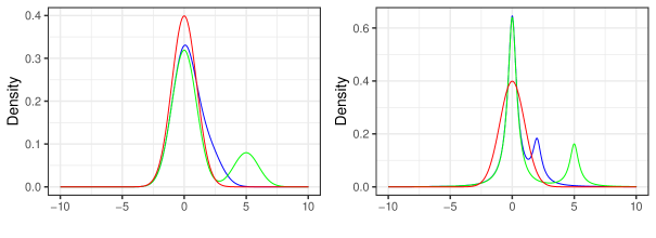
Conditions (i)–(v) help prove the consistency of the variance estimators and the mode of the regression coefficients. By assuming that the errors follow the normal distributions (Condition (iii)), we can integrate all the relevant covariate information in a single parameter ρ^^𝜌\hat{\rho}, which facilitates the establishment of the consistency of the kernel density estimation and hence the estimator of mode. In the simulation studies, we also investigated the scenario of non-normal distribution. We use an example to illustrate Condition (vi). In particular, we assume that n​αi𝑛subscript𝛼𝑖\sqrt{n}\alpha_{i} follows a discrete distribution with ℙ​(n​αi=an,l)=Ο€lℙ𝑛subscript𝛼𝑖subscriptπ‘Žπ‘›π‘™subscriptπœ‹π‘™\mathbb{P}(\sqrt{n}\alpha_{i}=a_{n,l})=\pi_{l} for l=0,1𝑙01l=0,1, where an,0=0subscriptπ‘Žπ‘›00a_{n,0}=0, an,1β‰ 0subscriptπ‘Žπ‘›10a_{n,1}\neq 0, Ο€l>0subscriptπœ‹π‘™0\pi_{l}>0, and Ο€0+Ο€1=1subscriptπœ‹0subscriptπœ‹11\pi_{0}+\pi_{1}=1. To reflect the sparsity, Ο€0subscriptπœ‹0\pi_{0} is set to be 0.80.80.8. We choose an,1=2subscriptπ‘Žπ‘›12a_{n,1}=2 and 555 representing weak and strong signals, respectively. We consider two cases for the error variance: (i) Οƒi=1subscriptπœŽπ‘–1\sigma_{i}=1; (ii) Οƒi∼IG​(a,b)similar-tosubscriptπœŽπ‘–IGπ‘Žπ‘\sigma_{i}\sim\text{IG}(a,b), i.e., ΟƒisubscriptπœŽπ‘–\sigma_{i} follows the inverse-gamma distribution with the shape parameter aπ‘Ža and scale parameter b𝑏b. As seen from Fig. 5, when the signal strength is weak, the mode of n​αi+ρ​Ρi​s𝑛subscriptπ›Όπ‘–πœŒsubscriptπœ€π‘–π‘ \sqrt{n}\alpha_{i}+\sqrt{\rho}\varepsilon_{is} slightly deviates from 0 as the blue curve in the left panel indicates. For strong signals, the mode is exactly equal to zero. As shown in [43], Condition (vii) is fulfilled by many commonly used kernels such as the Gaussian kernel and the uniform kernel on [βˆ’1,1]11[-1,1]. Condition (ix) allows the number of taxa to be exponentially larger than the sample size. Condition (x) ensures the existence of a cut-off value to control the FDR at level qπ‘žq. A similar assumption was imposed in Theorem 4 of [44].

5.6 Detailed setups for numerical studies

The differential taxa were randomly drawn from the entire set. In particular, let Hi=0subscript𝐻𝑖0H_{i}=0 if the i𝑖ith taxon is differentially abundant and Hi=1subscript𝐻𝑖1H_{i}=1 otherwise. The underlying truth Hisubscript𝐻𝑖H_{i} was generated from

Hi∼i.i.d.Bernoulli​(Ξ³).superscriptsimilar-toi.i.d.subscript𝐻𝑖Bernoulli𝛾H_{i}\sim^{\text{i.i.d.}}\text{Bernoulli}(\gamma).

We simulated two levels of signal density (i.e., percentage of differential taxa) γ𝛾\gamma = 5%, 20%, roughly corresponding to sparse and dense signals. We assumed that the baseline absolute abundance Xi​s(0)superscriptsubscript𝑋𝑖𝑠0X_{is}^{(0)} follows

log⁑(Xi​s(0))∼i.i.d.N​(Ξ²i(0),Οƒi2),superscriptsimilar-toi.i.d.superscriptsubscript𝑋𝑖𝑠0𝑁superscriptsubscript𝛽𝑖0superscriptsubscriptπœŽπ‘–2\displaystyle\log\left(X_{is}^{(0)}\right)\sim^{\text{i.i.d.}}N\left(\beta_{i}^{(0)},\sigma_{i}^{2}\right),

and correspondingly the absolute abundance Xi​ssubscript𝑋𝑖𝑠X_{is} were draw based on

log⁑(Xi​s)∼i.i.d.N​(Ξ²i(0)+us​αi+𝐜sβŠ€β€‹πœ·iβˆ’(0),Οƒi2),superscriptsimilar-toi.i.d.subscript𝑋𝑖𝑠𝑁superscriptsubscript𝛽𝑖0subscript𝑒𝑠subscript𝛼𝑖superscriptsubscriptπœπ‘ topsuperscriptsubscriptπœ·π‘–0superscriptsubscriptπœŽπ‘–2\displaystyle\log(X_{is})\sim^{\text{i.i.d.}}N\left(\beta_{i}^{(0)}+u_{s}\alpha_{i}+\mathbf{c}_{s}^{\top}\boldsymbol{\beta}_{i}^{-(0)},\sigma_{i}^{2}\right),

where 𝜷iβˆ’(0)superscriptsubscriptπœ·π‘–0\boldsymbol{\beta}_{i}^{-(0)} represents the coefficients of the confounders, i=1,…,m𝑖1β€¦π‘ši=1,\dots,m. Let

Ο€i​s(0)=Xi​s(0)βˆ‘j=1mXj​s(0)andΟ€i​s=Xi​sβˆ‘j=1mXj​s.formulae-sequencesuperscriptsubscriptπœ‹π‘–π‘ 0superscriptsubscript𝑋𝑖𝑠0superscriptsubscript𝑗1π‘šsuperscriptsubscript𝑋𝑗𝑠0andsubscriptπœ‹π‘–π‘ subscript𝑋𝑖𝑠superscriptsubscript𝑗1π‘šsubscript𝑋𝑗𝑠\displaystyle\pi_{is}^{(0)}=\frac{X_{is}^{(0)}}{\sum_{j=1}^{m}X_{js}^{(0)}}\quad\mbox{and}\quad\pi_{is}=\frac{X_{is}}{\sum_{j=1}^{m}X_{js}}.

The observed OTUs data were simulated by

(Y1​s,…,Ym​s)∼i.i.d.Multinomial​(Ns,Ο€1​s,…,Ο€m​s).superscriptsimilar-toi.i.d.subscriptπ‘Œ1𝑠…subscriptπ‘Œπ‘šπ‘ Multinomialsubscript𝑁𝑠subscriptπœ‹1𝑠…subscriptπœ‹π‘šπ‘ \displaystyle(Y_{1s},\dots,Y_{ms})\sim^{\text{i.i.d.}}\text{Multinomial}(N_{s},\pi_{1s},\dots,\pi_{ms}).

To create a power curve, we included six effect sizes labeled as {1,2,…,6}12…6\{1,2,...,6\} in the figures. We made the effect sizes have the same signs for differential taxa (i.e., the differential taxa have the same direction of change), creating a relatively strong compositional effect. Since low-abundance taxa have much less statistical power, we up-weighted their effects so that the power will not be dominated by those abundant ones. Specifically, for a randomly drawn differential taxon i𝑖i, we set

Ξ±i={log⁑(2​μ)​𝕀​(π¯i(0)>0.005)+log⁑{2​μ​(0.005/π¯i(0))1/3}​𝕀​(π¯i(0)≀0.005)​ for ​n=50,log⁑(ΞΌ)​𝕀​(π¯i(0)>0.005)+log⁑{μ​(0.005/π¯i(0))1/3}​𝕀​(π¯i(0)≀0.005)​ for ​n=200,subscript𝛼𝑖casesotherwise2πœ‡π•€subscriptsuperscriptΒ―πœ‹0𝑖0.0052πœ‡superscript0.005superscriptsubscriptΒ―πœ‹π‘–013𝕀subscriptsuperscriptΒ―πœ‹0𝑖0.005Β for 𝑛50otherwiseπœ‡π•€subscriptsuperscriptΒ―πœ‹0𝑖0.005πœ‡superscript0.005superscriptsubscriptΒ―πœ‹π‘–013𝕀subscriptsuperscriptΒ―πœ‹0𝑖0.005Β for 𝑛200\displaystyle\alpha_{i}=\begin{cases}&\log(2\mu)\mathbb{I}\left(\bar{\pi}^{(0)}_{i}>0.005\right)+\log\left\{2\mu\left(0.005/\bar{\pi}_{i}^{(0)}\right)^{{1}/{3}}\right\}\mathbb{I}\left(\bar{\pi}^{(0)}_{i}\leq 0.005\right)\text{ for }n=50,\\ &\log(\mu)\mathbb{I}\left(\bar{\pi}^{(0)}_{i}>0.005\right)+\log\left\{\mu\left(0.005/\bar{\pi}_{i}^{(0)}\right)^{{1}/{3}}\right\}\mathbb{I}\left(\bar{\pi}^{(0)}_{i}\leq 0.005\right)\text{ for }n=200,\end{cases}

where ΞΌπœ‡\mu is equally spaced on [1.05,2]1.052[1.05,2] and π¯i(0)=βˆ‘s=1nΟ€i​s(0)/nsuperscriptsubscriptΒ―πœ‹π‘–0superscriptsubscript𝑠1𝑛superscriptsubscriptπœ‹π‘–π‘ 0𝑛\bar{\pi}_{i}^{(0)}=\sum_{s=1}^{n}\pi_{is}^{(0)}/n. We considered three cases for the covariate and confounders:

  • C0.

    A binary covariate. us∼i.i.d.Bernoulli​(1/2)superscriptsimilar-toi.i.d.subscript𝑒𝑠Bernoulli12u_{s}\sim^{\text{i.i.d.}}\text{Bernoulli}(1/2) and no confounder.

  • C1.

    A continuous covariate. us∼i.i.d.N​(0,1)superscriptsimilar-toi.i.d.subscript𝑒𝑠𝑁01u_{s}\sim^{\text{i.i.d.}}N(0,1) and no confounder.

  • C2.

    A binary covariate of interest and two confounders. us∼Bernoulli​({1+exp⁑(βˆ’0.5​cs​1βˆ’0.5​cs​2)}βˆ’1)similar-tosubscript𝑒𝑠Bernoullisuperscript10.5subscript𝑐𝑠10.5subscript𝑐𝑠21u_{s}\sim\text{Bernoulli}(\{1+\exp(-0.5c_{s1}-0.5c_{s2})\}^{-1}) independently, where cs​1subscript𝑐𝑠1c_{s1} and cs​2subscript𝑐𝑠2c_{s2} are confounders (i.e., 𝐜s=(cs​1,cs​2)⊀subscriptπœπ‘ superscriptsubscript𝑐𝑠1subscript𝑐𝑠2top\mathbf{c}_{s}=(c_{s1},c_{s2})^{\top}). In the above, cs​1subscript𝑐𝑠1c_{s1} is specified to independently follow the Rademacher distribution and cs​2∼i.i.d.N​(0,1)superscriptsimilar-toi.i.d.subscript𝑐𝑠2𝑁01c_{s2}\sim^{\text{i.i.d.}}N(0,1). The corresponding coefficients of the confounders 𝜷iβˆ’(0)=(Ξ²i(1),Ξ²i(2))⊀superscriptsubscriptπœ·π‘–0superscriptsubscriptsuperscript𝛽1𝑖subscriptsuperscript𝛽2𝑖top\boldsymbol{\beta}_{i}^{-(0)}=(\beta^{(1)}_{i},\beta^{(2)}_{i})^{\top}, i=1,…,m𝑖1β€¦π‘ši=1,\dots,m, were independently generated from a 2-dimensional normal distribution with mean (1,2)⊀superscript12top(1,2)^{\top} and variance 𝐈2subscript𝐈2\mathbf{I}_{2}, where 𝐈2subscript𝐈2\mathbf{I}_{2} denotes the 2 by 2 identity matrix.

The parameters Ξ²i(0)superscriptsubscript𝛽𝑖0\beta_{i}^{(0)}, Οƒi2superscriptsubscriptπœŽπ‘–2\sigma_{i}^{2}, and Nssubscript𝑁𝑠N_{s} were generated based on the estimation for a real dataset (COMBO) from the study of the gut microbiota in a general population [45], which consists of 98 samples and 6674 taxa. We only used its 500 most abundant taxa. Since Ξ²i(0)superscriptsubscript𝛽𝑖0\beta_{i}^{(0)} and Οƒi2superscriptsubscriptπœŽπ‘–2\sigma_{i}^{2} were not directly estimable using the relative abundance data, we estimated Ξ²i(0)βˆ’Ξ²j(0)superscriptsubscript𝛽𝑖0superscriptsubscript𝛽𝑗0\beta_{i}^{(0)}-\beta_{j}^{(0)} and Οƒi2+Οƒj2superscriptsubscriptπœŽπ‘–2superscriptsubscriptπœŽπ‘—2\sigma_{i}^{2}+\sigma_{j}^{2} based on the pairwise log ratios, forced some Ξ²i(0)superscriptsubscript𝛽𝑖0\beta_{i}^{(0)}’s to be zeros to obtain the estimators of Ξ²1(0),…,Ξ²m(0)superscriptsubscript𝛽10…superscriptsubscriptπ›½π‘š0\beta_{1}^{(0)},\dots,\beta_{m}^{(0)}, and derived Οƒi2superscriptsubscriptπœŽπ‘–2\sigma_{i}^{2} from the values of {Οƒi2+Οƒj2}i,jsubscriptsuperscriptsubscriptπœŽπ‘–2superscriptsubscriptπœŽπ‘—2𝑖𝑗\{\sigma_{i}^{2}+\sigma_{j}^{2}\}_{i,j}. We assume that the library size for each sample follows the negative binomial distribution

Ns∼i.i.d.NB​(7645,5.3),superscriptsimilar-toi.i.d.subscript𝑁𝑠NB76455.3N_{s}\sim^{\text{i.i.d.}}\text{NB}(7645,5.3),

where the mean and dispersion parameters were estimated based on the combo data. The resulting sparsity (percent of zeros) of the count matrix is around 65%–75%.

In addition to the basic setting (S0, log normal abundance distribution), we designed seven other settings to study the robustness of the proposed method. Specifically, on top of S0 and C0 (a binary covariate), we studied

  • S1.

    zero-inflated absolute abundances. The microbiome data contains excessive zeros and many zeros in the microbiome data can be explained by insufficient sampling [46] since majority of the taxa are of low-abundance. However, it is also possible that zeros are due to physical absence of the taxa [47]. To study the effect of zero inflation on differential abundance analysis, we randomly forced 30% of the absolute abundance data to be 0.

  • S2.

    Correlated absolute abundances. Existing differential abundance analysis methods assume independence among taxa. However, in practice, taxa are interconnected forming networks [48]. It is interesting to see if the methods compared are robust to the correlations among the taxa. In this setting, we simulated block-correlation structure by dividing the 500 taxa into 25 equal-sized blocks. Within each block, we further divided the block into 2 by 2 sub-blocks and simulated equal positive correlations (0.5) within each sub-block and equal negative correlations (βˆ’0.50.5-0.5) between the two sub-blocks. This mimics the scenario that there are mutualistic relationships within the group and competitive relationships between groups.

  • S3.

    Gamma abundance distribution. Although the log normal distribution has been widely used for modeling species abundance data, other models such as gamma distribution are also possible [49]. We thus did additional simulation studies using the gamma distribution. Let Xi​s(0)∼i.i.d.Gamma​(Ξ·i(0),1)superscriptsimilar-toi.i.d.superscriptsubscript𝑋𝑖𝑠0Gammasuperscriptsubscriptπœ‚π‘–01X_{is}^{(0)}\sim^{\text{i.i.d.}}\text{Gamma}(\eta_{i}^{(0)},1) and Xi​s∼i.i.d.Gamma​(Ξ·i(0)​exp⁑(us​αi+𝐜sβŠ€β€‹πœ·iβˆ’(0)),1)superscriptsimilar-toi.i.d.subscript𝑋𝑖𝑠Gammasuperscriptsubscriptπœ‚π‘–0subscript𝑒𝑠subscript𝛼𝑖superscriptsubscriptπœπ‘ topsuperscriptsubscriptπœ·π‘–01X_{is}\sim^{\text{i.i.d.}}\text{Gamma}(\eta_{i}^{(0)}\exp(u_{s}\alpha_{i}+\mathbf{c}_{s}^{\top}\boldsymbol{\beta}_{i}^{-(0)}),1). Similarly, we estimated Ξ·i(0)superscriptsubscriptπœ‚π‘–0\eta_{i}^{(0)} from the COMBO data, where we first estimated the baseline proportion Ο€i(0)superscriptsubscriptπœ‹π‘–0\pi_{i}^{(0)} based on the Dirichlet-multinomial distribution using the R function dirmult and set the over-dispersion parameter ΞΈ(0)superscriptπœƒ0\theta^{(0)} to be 0.003, then let Ξ·i(0)=Ο€i(0)​(1/ΞΈ(0)βˆ’1)superscriptsubscriptπœ‚π‘–0subscriptsuperscriptπœ‹0𝑖1superscriptπœƒ01\eta_{i}^{(0)}=\pi^{(0)}_{i}(1/\theta^{(0)}-1).

  • S4.

    Smaller mπ‘šm. In microbiome data, each taxon can be assigned a taxonomic lineage and taxa abundances can be aggregated at different taxonomic ranks. Differential abundance analysis at higher ranks such as family and genus is also routinely performed. At the higher ranks, the number of taxa is much smaller. We thus studied a small number of taxa (m=50π‘š50m=50) to see if the proposed method is robust to a small mπ‘šm. In this setting, we randomly chose 50 elements from 𝜷(0)=(Ξ²1(0),…,Ξ²500(0))⊀superscript𝜷0superscriptsuperscriptsubscript𝛽10…superscriptsubscript𝛽5000top\boldsymbol{\beta}^{(0)}=(\beta_{1}^{(0)},...,\beta_{500}^{(0)})^{\top} and 𝝈2=(Οƒ12,…,Οƒ5002)⊀superscript𝝈2superscriptsuperscriptsubscript𝜎12…superscriptsubscript𝜎5002top\boldsymbol{\sigma}^{2}=(\sigma_{1}^{2},...,\sigma_{500}^{2})^{\top} in each simulation run. We set Ns∼NB​(1500,5.3)similar-tosubscript𝑁𝑠NB15005.3N_{s}\sim\text{NB}(1500,5.3).

  • S5.

    Smaller n𝑛n. In pilot microbiome studies, the sample sizes are usually small. It is interesting to study the performance of the methods at a much smaller sample size. We studied n=20, 30𝑛2030n=20,\;30, and used the same effect size as n=50𝑛50n=50.

  • S6.

    10-fold difference in library size. When the microbiome samples are not fully randomized in sequencing, it is likely that samples of the two groups end up in two separate sequencing runs leading to very different library sizes for the two groups. Since the presence/absence of a taxon strongly depends on the library size, the differential library size will confound the two-sample comparison, especially for those rare taxa [25]. To create differential library sizes, we generated the library size from Ns∼NB​(5000,5.3)similar-tosubscript𝑁𝑠NB50005.3N_{s}\sim\text{NB}(5000,5.3) and Ns∼NB​(50000,5.3)similar-tosubscript𝑁𝑠NB500005.3N_{s}\sim\text{NB}(50000,5.3) for the two groups, respectively.

  • S7.

    Negative bionomial abundance distribution. DESeq2 and edgeR assume negative binomial distribution for the counts, thus we included one more simulation setting, where we generated the counts from the negative binomial distribution. Let Xi​s(0)∼i.i.d.NB​(exp​(7645​κi(0)),ΞΈi(0))superscriptsimilar-toi.i.d.superscriptsubscript𝑋𝑖𝑠0NBexp7645superscriptsubscriptπœ…π‘–0superscriptsubscriptπœƒπ‘–0X_{is}^{(0)}\sim^{\text{i.i.d.}}\text{NB}(\text{exp}(7645\kappa_{i}^{(0)}),\theta_{i}^{(0)}) and Yi​s∼i.i.d.NB​(exp​(Ns​κi(0)+us​αi+𝐜sβŠ€β€‹πœ·iβˆ’(0)),ΞΈi(0))superscriptsimilar-toi.i.d.subscriptπ‘Œπ‘–π‘ NBexpsubscript𝑁𝑠superscriptsubscriptπœ…π‘–0subscript𝑒𝑠subscript𝛼𝑖superscriptsubscriptπœπ‘ topsuperscriptsubscriptπœ·π‘–0superscriptsubscriptπœƒπ‘–0Y_{is}\sim^{\text{i.i.d.}}\text{NB}(\text{exp}(N_{s}\kappa_{i}^{(0)}+u_{s}\alpha_{i}+\mathbf{c}_{s}^{\top}\boldsymbol{\beta}_{i}^{-(0)}),\theta_{i}^{(0)}). Similarly, we estimated the ΞΊi(0)superscriptsubscriptπœ…π‘–0\kappa_{i}^{(0)} (regression coefficient for the library size with respect to the log of the count of i𝑖ith taxon) and ΞΈi(0)superscriptsubscriptπœƒπ‘–0\theta_{i}^{(0)} (dispersion parameter) from the COMBO data using the R function glm.nb.

  • S8.

    Mixed-effect model. We considered two scenarios: Pre-treatment and post-treatment comparison (S8.1) and Replicate sampling (S8.2). Under S8.1, for n=50𝑛50n=50 (or 200), we simulated 252525 (or 100) subjects and each has paired pre-treatment and post-treatment samples. The aim is to detect taxa affected by treatment. Under S8.2, each subject has multiple measurements. For n=50𝑛50n=50 (or 200), we generated 25 (or 50) subjects with each having 2 (or 4) replicates. Specifically, we let

    log⁑(Xi​s)∼𝐫sβŠ€β€‹πœΈi+N​(Ξ²i(0)+us​αi+𝐜sβŠ€β€‹πœ·iβˆ’(0),Οƒi2),similar-tosubscript𝑋𝑖𝑠superscriptsubscript𝐫𝑠topsubscriptπœΈπ‘–π‘superscriptsubscript𝛽𝑖0subscript𝑒𝑠subscript𝛼𝑖superscriptsubscriptπœπ‘ topsuperscriptsubscriptπœ·π‘–0superscriptsubscriptπœŽπ‘–2\log(X_{is})\sim\mathbf{r}_{s}^{\top}\boldsymbol{\gamma}_{i}+N(\beta_{i}^{(0)}+u_{s}\alpha_{i}+\mathbf{c}_{s}^{\top}\boldsymbol{\beta}_{i}^{-(0)},\sigma_{i}^{2}),

    where 𝐫ssubscript𝐫𝑠\mathbf{r}_{s} has one element equal to 1 and all the others equal to 0 indicating the subject ID of sample s𝑠s. Each element of 𝜸isubscriptπœΈπ‘–\boldsymbol{\gamma}_{i} follows N​(0,Ο„i2)𝑁0superscriptsubscriptπœπ‘–2N(0,\tau_{i}^{2}) independently, where we let Ο„i2=ai​σi2superscriptsubscriptπœπ‘–2subscriptπ‘Žπ‘–superscriptsubscriptπœŽπ‘–2\tau_{i}^{2}=a_{i}\sigma_{i}^{2} with ai∼Unif​([0,1])similar-tosubscriptπ‘Žπ‘–Unif01a_{i}\sim\text{Unif}([0,1]).

Declarations

Ethics approval and consent to participate

Not applicable.

Consent for publication

Not applicable.

Availability of data and materials

LinDA is implemented as the linda function in the CRAN R package MicrobiomeStat (https://CRAN.R-project.org/package=MicrobiomeStat). The LinDA package is also available at GitHub (https://github.com/zhouhj1994/LinDA). The entire codes and data for generating the presented results are available at the repository Zenodo (https://doi.org/10.5281/zenodo.6326019) and at GitHub (https://github.com/zhouhj1994/LinDA-manuscript-result) under MIT License. The CDI, IBD, RA, SMOKE and COMBO datasets are from [29, 30, 31, 32, 45], respectively.

Competing interests

The authors declare no competing interests.

Funding

This work was supported by National Institute of Health R01GM144351 (Chen & Zhang), National Science Foundation DMS-1830392, DMS2113359, DMS1811747 (Zhang & Zhou) and National Science Foundation DMS2113360 and Mayo Clinic Center for Individualized Medicine (Chen).

Authors’ contributions

J.C. and X.Z. conceived, designed and supervised the work together. X.Z. developed the method. X.Z., K.H and H.Z. performed the theoretical analysis. H.Z. and J.C. performed the evaluation and developed the software. J.C., H.Z., X.Z. and K.H wrote and revised the manuscript together.

Acknowledgements

Not applicable.

Figures and Tables

Fig. 1 Performance comparison (S0C0: log normal abundance distribution, a binary covariate). Empirical false discovery rate (A) and true positive rates (B) were averaged over 100 simulation runs. Error bars (A) represent the 95% confidence intervals (CIs) of the method LinDA and the dashed horizontal line indicates the target FDR level of 0.05.

Fig. 2 Performance comparison (S3C0: gamma abundance distribution, a binary covariate). Empirical false discovery rate (A) and true positive rates (B) were averaged over 100 simulation runs. Error bars (A) represent the 95% CIs of the method LinDA and the dashed horizontal line indicates the target FDR level of 0.05.

Fig. 3 Number of discoveries v.s. target FDR level (0.01–0.25) for the three real datasets.

Fig. 4 Overlaps of differential taxa with target FDR level of 0.1 for the four real datasets.

Fig. 5 Density of n​αi+Ξ΅i​s𝑛subscript𝛼𝑖subscriptπœ€π‘–π‘ \sqrt{n}\alpha_{i}+\varepsilon_{is}. The panels on the left and right correspond to Οƒi=1subscriptπœŽπ‘–1\sigma_{i}=1 and Οƒi∼IG​(2,1)similar-tosubscriptπœŽπ‘–IG21\sigma_{i}\sim\text{IG}(2,1) respectively, where IG denotes the inverse-gamma distribution. The red curve is the density of the standard normal distribution. The blue and green curves are the densities of n​αi+Ξ΅i​s𝑛subscript𝛼𝑖subscriptπœ€π‘–π‘ \sqrt{n}\alpha_{i}+\varepsilon_{is} with ℙ​(n​αi=0)=0.8ℙ𝑛subscript𝛼𝑖00.8\mathbb{P}(\sqrt{n}\alpha_{i}=0)=0.8 and ℙ​(n​αi=2)=0.2ℙ𝑛subscript𝛼𝑖20.2\mathbb{P}(\sqrt{n}\alpha_{i}=2)=0.2, and ℙ​(n​αi=0)=0.8ℙ𝑛subscript𝛼𝑖00.8\mathbb{P}(\sqrt{n}\alpha_{i}=0)=0.8 and ℙ​(n​αi=5)=0.2ℙ𝑛subscript𝛼𝑖50.2\mathbb{P}(\sqrt{n}\alpha_{i}=5)=0.2, respectively.

Table 1 Runtime (in second) comparison under different settings (R version 4.0.3 (2020-10-10); Platform: x86_64-pc-linux-gnu (64-bit); CPU: E5-2670 v2 @ 2.50GHz; Memory: 67.7 GB). The result is based on one simulation run. Theβ€œelapsed” from the R command system.time() was used.

Table 2 Characteristics of four real microbiome datasets. NORA represents new-onset untreated rheumatoid arthritis. The second and the third columns respectively list the number of taxa and sample size of each filtered dataset (prevalence β‰₯\geq 10%, library size β‰₯\geq 1000).

Supplementary material

Additional file 1: supplementary notes. Table S1 lists some robust normalization methods [11, 12, 13, 14]. Lemmas S1 – S4 present intermediate results for proving Theorem 1. The proof depends on some useful results from [Zhou:2021, 51, 52, 53].

Additional file 2: supplementary figures. Fig. S1 and S2 compare the proposed method LinDA with different zero-handling approaches under settings S6C0 and S0C0. Fig. S3 depicts the results of LinDA, CLR-OLS and MaAsLin2 with different normalization approaches under setting S0C0. Fig. S4–S10 and S12–S14 show the results of settings S0C1, S0C2, S1C0, S2C0, S4C0, S5C0, S6C0, S7C0, S8.1C0, and S8.2C0, respectively. The comparison between disabling and enabling zero treatment of the ANCOM-BC method is depicted in Fig. S11 under setting S6C0. Fig. S15 shows the results of setting S0C0 with stronger compositional effects. Fig. S16–S19 show the effect size plots and volcano plots for the four datasets (CDI, IBD, RA, and SMOKE) respectively. Fig. S20–S30 present the full result of all methods under different simulation settings.

References

  • Fan & Pedersen [2021] Fan, Y. and Pedersen, O. (2021). Gut microbiota in human metabolic health and disease. Nature Reviews Microbiology 19, 55–71.
  • Valdes et al. [2018] Valdes, A. M., Walter, J., Segal, E., and Spector, T.Β M. (2018). Role of the gut microbiota in nutrition and health. BMJ 361, k2179.
  • Edgar [2013] Edgar, R. C. (2013). UPARSE: highly accurate OTU sequences from microbial amplicon reads. Nature Methods 10, 996–998.
  • Callahan et al. [2016] Callahan, B. J., McMurdie, P. J., Rosen, M. J., Han, A. W., Johnson, A. J. A., and Holmes, S. P. (2016). DADA2: High-resolution sample inference from Illumina amplicon data. Nature Methods 13, 581–583.
  • Segata et al. [2012] Segata, N., Waldron, L., Ballarini, A., Narasimhan, V., Jousson, O., and Huttenhower, C. (2012). Metagenomic microbial community profiling using unique clade-specific marker genes. Nature Methods 9, 811–814.
  • Gloor et al. [2017] Gloor, G. B., Macklaim, J. M., Pawlowsky-Glahn, V., and Egozcue, J. J (2017). Microbiome datasets are compositional: and this is not optional. Frontiers in Microbiology 8, 2224.
  • Tsilimigras & Fodor [2016] Tsilimigras, M. C. B. and Fodor, A. A. (2016). Compositional data analysis of the microbiome: fundamentals, tools, and challenges. Annals of Epidemiology 26, 330–335.
  • Morton et al. [2019] Morton, J. T., Marotz, C., Washburne, A., Silverman, J., Zaramela, L. S., Edlund, A., Zengler, K., and Knight, R. (2019). Establishing microbial composition measurement standards with reference frames. Nature communications 10, 2719.
  • Xiao et al. [2018:1] Xiao, J., Chen, L., Yu, Y., Zhang, X., and Chen, J. (2018). A phylogeny-regularized sparse regression model for predictive modeling of microbial community data. Frontiers in Microbiology 9, 3112.
  • Xiao et al. [2018:2] Xiao, J., Chen, L., Johnson, S., Yu, Y., Zhang, X., and Chen, J. (2018). Predictive modeling of microbiome data using a phylogeny-regularized generalized linear mixed model. Frontiers in Microbiology 9, 1391.
  • Robinson & Oshlack [2010] Robinson, M. D. and Oshlack, A. (2010). A scaling normalization method for differential expression analysis of RNA-seq data. Genome Biology 11, R25.
  • Anders & Huber [2010] Anders, S. and Huber, W. (2010). Differential expression analysis for sequence count data. Genome Biology 11, R106.
  • Paulson et al. [2013] Paulson, J. N., Stine, O. C., Bravo, H. C., and Pop, M. (2013). Differential abundance analysis for microbial marker-gene surveys. Nature Methods 10, 1200–1202.
  • Chen et al. [2018] Chen, L., Reeve, J., Zhang, L., Huang, S., Wang, X., and Chen, J. (2018). GMPR: A robust normalization method for zero-inflated count data with application to microbiome sequencing data. PeerJ 6, e4600.
  • Robinson et al. [2010] Robinson, M. D., McCarthy, D. J., and Smyth, G. K. (2010). edgeR: a Bioconductor package for differential expression analysis of digital gene expression data. Bioinformatics 26, 139–140.
  • Love et al. [2014] Love, M. I., Huber, W., and Anders, S. (2014). Moderated estimation of fold change and dispersion for RNA-seq data with DESeq2. Genome Biology 15, 550.
  • Chen et al. [2018] Chen, J., King, E., Deek, R., Wei, Z., Yu, Y., Grill, D., Ballman, K., and Stegle, O. (2018). An omnibus test for differential distribution analysis of microbiome sequencing data. Bioinformatics 34, 643–651.
  • Mallick et al. [2020] Mallick H., Rahnavard A., Mclver L. J., Ma S., Zhang Y., Nguyen L. H., Tickle T. L., Weingart G., Ren B., Schwager E. H., et al. (2021). Multivariable association discovery in population-scale meta-omics studies. PLoS computational biology 17, e1009442.
  • Sohn et al. [2015] Sohn, M. B., Du, R., and An, L. (2015). A robust approach for identifying differentially abundant features in metagenomic samples. Bioinformatics 31, 2269–2275.
  • Brill et al. [2020] Brill, B., Amir, A., and Heller, R. (2020). Testing for differential abundance in compositional counts data, with application to microbiome studies. arXiv preprint arXiv:1904.08937.
  • Aitchison [1986] Aitchison J. (1986). The statistical analysis of compositional data. Chapman and Hall.
  • Fernandes et al. [2014] Fernandes, A. D., Reid, J. N., Macklaim, J. M., McMurrough, T. A., Edgell, D. R., and Gloor, G. B. (2014). Unifying the analysis of high-throughput sequencing datasets: characterizing RNA-seq, 16S rRNA gene sequencing and selective growth experiments by compositional data analysis. Microbiome 2, 15.
  • Mandal et al. [2015] Mandal, S., Treuren, W. V., White, R. A., EggesbΓΈ, M., Knight, R., and Peddada, S. D. (2015). Analysis of composition of microbiomes: a novel method for studying microbial composition. Microbial Ecology in Health & Disease 26, 27663.
  • Lin & Peddada [2020] Lin, H. and Peddada, S. D. (2020). Analysis of compositions of microbiomes with bias correction. Nature Communications 11, 3514.
  • Weiss et al. [2017] Weiss, S., Xu, Z. Z., Peddada, S., Amir, A., Bittinger, K., Gonzalez, A., Lozupone, C., Zaneveld, J. R., Va´´a\acute{\text{a}}zquez-Baeza, Y., Birmingham, A., et al. (2017). Normalization and microbial differential abundance strategies depend upon data characteristics. Microbiome 5, 27.
  • Hawinkel et al. [2019] Hawinkel, S., Mattiello, F., Bijnens, L., and Thas, O. (2019). A broken promise: microbiome differential abundance methods do not control the false discovery rate. Briefings in Bioinformatics 20, 210–221.
  • Faust et al. [2015] Faust, K., Lahti, L., Gonze, D., Vos, W. M. D., and Raes, J. (2015). Metagenomics meets time series analysis: unraveling microbial community dynamics. Current Opinion in Microbiology 25, 56–66.
  • Lewis et al. [2015] Lewis, J. D., Chen, E. Z., Baldassano, R. N., Otley, A. R., Griffiths, A. M., Lee, D., Bittinger, K., Bailey, A., Friedman, E. S., Hoffmann, C., et al. (2015). Inflammation, antibiotics, and diet as environmental stressors of the gut microbiome in pediatric crohn’s Disease. Cell Host & Microbe 18, 489–500.
  • Schubert et al. [2014] Schubert, A. M., Rogers, M.Β A.Β M., Ring, C., Mogle, J., Petrosino, J.Β P., Young, V. B., Aronoff, D. M., and Schloss, P. D. (2014). Microbiome data distinguish patients with clostridium difficile infection and non-C. difficile-associated diarrhea from healthy controls. mBio 5, e01021-14.
  • Morgan et al. [2012] Morgan, X. C., Tickle, T. L., Sokol, H., Gevers, D., Devaney, K. L., Ward, D. V., Reyes, J. A., Shah, S. A., LeLeiko, N., Snapper, S. B., et al. (2012). Dysfunction of the intestinal microbiome in inflammatory bowel disease and treatment. Genome Biology 13, R79.
  • Scher et al. [2013] Scher, J. U., Sczesnak, A., Longman, R. S., Segata, N., Ubeda, C., Bielski, C., Rostron, T., Cerundolo, V., Pamer, E. G., Abramson, S. B., et al. (2013). Expansion of intestinal Prevotella copri correlates with enhanced susceptibility to arthritis. eLife 2, e01202.
  • Charlson et al. [2010] Charlson, E. S., Chen, J., Custers-Allen, R., Bittinger, K., Li, H., Sinha, R., Hwang, J., Bushman, F. D., and Collman, R. G. (2010). Disordered microbial communities in the upper respiratory tract of cigarette smokers. PloS One 5, e15216.
  • Gonzalez [2018] Gonzalez, A., Navas-Molina, J. A., Kosciolek, T., McDonald, D., Va´´a\acute{\text{a}}zquez-Baeza, Y., Ack- ermann, G., DeReus, J., Janssen, S., Swafford, A. D., Orchanian, S. B., et al. (2018). Qiita: rapid, web-enabled microbiome meta-analysis. Nature Methods 15, 796–798.
  • Lex et al. [2014] Lex, A., Gehlenborg, N., Strobelt, H., Vuillemot, R., and Pfister, H. (2014). UpSet: visualization of intersecting sets. IEEE Transactions on Visualization and Computer Graphics 20, 1983–1992.
  • Bates et al. [2015] Bates, D., Ma¨¨a\ddot{\text{a}}chler, M., Bolker, B. M., and Walker, S. C. (2015). Fitting linear mixed-effects models using lme4. Journal of Statistical Software 67.
  • Carpenter & Kenward [2012] Carpenter, J. and Kenward, M. (2012). Multiple imputation and its application. John Wiley & Sons.
  • Quinn et al. [2018] Quinn, T. P., Erb, I., Richardson, M. F., and Crowley, T. M. (2018). Understanding sequencing data as compositions: an outlook and review. Bioinformatics 34, 2870–2878.
  • Chen et al. [2012] Chen, J., Bittinger, K., Charlson, E. S., Hoffmann, C., Lewis, J., Wu, G. D., Collman, R. G., Bushman, F. D., and Li, H. (2012.) Associating microbiome composition with environmental covariates using generalized UniFrac distances. Bioinformatics, 28 2106–2113.
  • Chen & Zhang [2021] Chen, J. and Zhang, X. (2022). D-MANOVA: fast distance-based multivariate analysis of variance for large-scale microbiome association studies. Bioinformatics 38, 286–288.
  • Thorsen et al. [2016] Thorsen, J., Brejnrod, A., Mortensen, M., Rasmussen, M. A., Stokholm, J., Al-Soud, W. A., SΓΈrensen, S., Bisgaard, H., and Waage, J. (2016). Large-scale benchmarking reveals false discoveries and count transformation sensitivity in 16S rRNA gene amplicon data analysis methods used in microbiome studies. Microbiome 4, 62.
  • Zhou & Gallins [2019] Zhou, Y. H. and Gallins, P. (2019). A review and tutorial of machine learning methods for microbiome host trait prediction. Frontiers in Genetics 10, 579.
  • McDonald et al. [2018] McDonald, D., Hyde, E., Debelius, J. W., Morton, J. T., Gonzalez, A., Ackermann, G., Aksenov, A. A., Behsaz, B., Brennan, C., Chen, Y., et al. (2018). American Gut: an Open Platform for Citizen Science Microbiome Research. mSystems 3, e00031-18.
  • Parzen [1962] Parzen, E. (1962). On estimation of a probability density function and mode. Annals of Mathematical Statistics 33, 1065–1076.
  • Storey et al. [2004] Storey, J. D., Taylor, J. E., and Siegmund, D. (2004). Strong control, conservative point estimation and simultaneous conservative consistency of false discovery rates: a unified approach. Journal of the Royal Statistical Society, Series B 66, 187–205.
  • Wu et al. [2011] Wu, G. D., Chen, J., Hoffmann, C., Bittinger, K., Chen, Y.-Y., Keilbaugh, S. A., Bewtra, M., Knights, D., Walters, W. A., Knight, R., et al. (2011). Linking long-term dietary patterns with gut microbial enterotypes. Science 334, 105-108.
  • Silverman et al. [2020] Silverman, J. D., Roche, K., Mukherjee, S., and David, L. A. (2020). Naught all zeros in sequence count data are the same. Computational and Structural Biotechnology Journal 18, 2789–2798.
  • Kaul et al. [2017] Kaul, A., Mandal, S., Davidov, O., and Peddada, S. D. (2017). Analysis of microbiome data in the presence of excess zeros. Frontiers in Microbiology 8, 2114.
  • Kurtz et al. [2015] Kurtz, Z. D., Mu¨¨u\ddot{\text{u}}ller, C. L., Miraldi, E. R., Littman, D. R., Blaser, M. J., and Bonneau, R. A. (2015). Sparse and compositionally robust inference of microbial ecological networks. PLoS Computational Biology 11, e1004226.
  • Connolly [2014] Connolly, S. R., MacNeil, M. A., Caley, M. J., Knowlton, N., Cripps, E., Hisano, M., Thibaut, L. M., Bhattacharya, B. D., Benedetti-Cecchi, L., Brainard, R. E., et al. (2014). Commonness and rarity in the marine biosphere. Proceedings of the National Academy of Sciences 111, 8524–-8529.
  • Zhou et al. [2020] Zhou, H., Zhang, X., and Chen, J. (2021). Covariate adaptive family-wise error rate control for genome-wide association studies. Biometrika 108, 915–931.
  • Vershynin [2018] Vershynin, R. (2018). High-dimensional probability: An introduction with applications in data science. Cambridge University Press.
  • Wainwright [2019] Wainwright, M. J. (2019). High-dimensional statistics: A non-asymptotic viewpoint. Cambridge University Press.
  • Cao et al. [2021] Cao, H., Chen, J., and Zhang, X. (2021). Optimal false discovery rate control for large scale multiple testing with auxiliary information. The Annals of Statistics, forthcoming. https://web.stat.tamu.edu/Β zhangxiany/Order-FDR.pdf.
Refer to caption
Refer to caption
Fig. 1:
Refer to caption
Refer to caption
Fig. 2:
Refer to caption
Fig. 3:
Refer to caption
(a) CDI
Refer to caption
(b) IBD
Refer to caption
(c) RA
Refer to caption
(d) SMOKE
Fig. 4:
Refer to caption
Fig. 5:
Table 1:
S0C0 S0C1 S0C2
LinDA ANCOM-BC LinDA ANCOM-BC LinDA ANCOM-BC
m=500π‘š500m=500 n=200𝑛200n=200 0.4540.454\bf{0.454} 21.83521.83521.835 0.2180.218\bf{0.218} 22.05722.05722.057 0.2060.206\bf{0.206} 64.51964.51964.519
n=10000𝑛10000n=10000 6.8446.844\bf{6.844} 162.218162.218162.218 4.0434.043\bf{4.043} 163.552163.552163.552 5.0735.073\bf{5.073} 216.564216.564216.564
m=5000π‘š5000m=5000 n=200𝑛200n=200 1.5981.598\bf{1.598} 184.972184.972184.972 1.6071.607\bf{1.607} 162.611162.611162.611 1.6151.615\bf{1.615} 599.985599.985599.985
n=10000𝑛10000n=10000 28.25328.253\bf{28.253} 5,135.3935135.3935,135.393 15.31415.314\bf{15.314} 5,157.1485157.1485,157.148 15.49415.494\bf{15.494} 5,506.3535506.3535,506.353
Table 2:
mπ‘šm n𝑛n u𝑒u 𝐜𝐜\mathbf{c}
CDI 123 183 CDI/Diarrhea control (94 v.s. 89)
IBD 579 81 Crohn’s disease/Healthy (62 v.s. 19) Antibiotic use (n/y, 48 + 19 v.s. 14 + 0)
RA 438 72 NORA/Healthy (44 v.s. 28)
SMOKE 209 132 Smoke (n/y, 67 v.s. 65) Female/Male (31 + 16 v.s. 36 + 49)

Supplementary notes for β€œLinDA: linear models for differential abundance analysis of microbiome compositional data”

S1 Normalization approaches

Table S1: Some robust normalization methods
Method Description
Trimmed mean of M-values (TMM) [11, Robinson & Oshlack, 2010] TMM (in log scale) is the weighted mean of the log-ratio between the relative abundances and a referenced relative abundance after excluding the most abundant taxa and the taxa with the largest log-fold changes.
DESeq normalization (RLE) [12, Anders & Huber, 2010] In RLE, the normalizing factor is the median of the ratios between the counts and the geometric mean of the counts of all samples.
Cumulative-sum scaling (CSS) [13, Paulson et al., 2013] In CSS, counts are divided by the cumulative sum of counts, up to a quantile determined by a data-driven approach.
Geometric mean of pairwise ratios (GMPR) [14, Chen et al., 2018] GMPR is the geometric mean of the medians of the ratios between the pairs of counts of two samples, which reverses the order of the two steps in the RLE.

Note that the first number in the square brackets represents the reference number in the manuscript.

S2 Technical details

In the following, we use FX​(β‹…)subscript𝐹𝑋⋅F_{X}(\cdot) to denote the cumulative distribution function of a random variable X𝑋X. Denote by oβ„™msubscriptπ‘œsubscriptβ„™π‘šo_{\mathbb{P}_{m}} (Oβ„™msubscript𝑂subscriptβ„™π‘šO_{\mathbb{P}_{m}}), oβ„™nsubscriptπ‘œsubscriptℙ𝑛o_{\mathbb{P}_{n}} (Oβ„™nsubscript𝑂subscriptℙ𝑛O_{\mathbb{P}_{n}}), and oβ„™subscriptπ‘œβ„™o_{\mathbb{P}} (Oβ„™subscript𝑂ℙO_{\mathbb{P}}) the corresponding rates of convergence as mβ†’βˆžβ†’π‘šm\to\infty, nβ†’βˆžβ†’π‘›n\to\infty, and m,nβ†’βˆžβ†’π‘šπ‘›m,n\to\infty simultaneously, respectively. We first introduce some useful lemmas before proving Theorem 1.

Lemma S1.

Under Condition (i) in Theorem 1, we have

|ρ^βˆ’Ο|=oβ„™n​(1).^𝜌𝜌subscriptπ‘œsubscriptℙ𝑛1\displaystyle|\hat{\rho}-\rho|=o_{\mathbb{P}_{n}}(1).
Lemma S2.

Under Conditions (i), (ii), (iii), (v), and (ix) in Theorem 1, we have

maxi⁑|Οƒ^i2βˆ’Οƒi2|=oℙ​(1).subscript𝑖superscriptsubscript^πœŽπ‘–2superscriptsubscriptπœŽπ‘–2subscriptπ‘œβ„™1\displaystyle\max_{i}|\hat{\sigma}_{i}^{2}-\sigma_{i}^{2}|=o_{\mathbb{P}}(1).
Lemma S3.

Under Conditions (i)–(viii) in Theorem 1, we have

n​(Ξ±~βˆ’Ξ±Β―)=oℙ​(1).𝑛~𝛼¯𝛼subscriptπ‘œβ„™1\displaystyle\sqrt{n}(\tilde{\alpha}-\bar{\alpha})=o_{\mathbb{P}}(1).
Lemma S4.

Suppose Conditions (i)–(ix) in Theorem 1 are satisfied. Let m0subscriptπ‘š0m_{0} be the number of true null hypotheses and

Vm,n​(t)=βˆ‘i:Ξ±i=0𝕀​(|n​α^i|/ρ^​σ^i2>t),subscriptπ‘‰π‘šπ‘›π‘‘subscript:𝑖subscript𝛼𝑖0𝕀𝑛subscript^𝛼𝑖^𝜌superscriptsubscript^πœŽπ‘–2𝑑\displaystyle V_{m,n}(t)=\sum_{i:\alpha_{i}=0}\mathbb{I}\left(|\sqrt{n}\hat{\alpha}_{i}|/\sqrt{\hat{\rho}\hat{\sigma}_{i}^{2}}>t\right),
Sm,n​(t)=βˆ‘i=1m𝕀​(|n​α^i|/ρ^​σ^i2>t),subscriptπ‘†π‘šπ‘›π‘‘superscriptsubscript𝑖1π‘šπ•€π‘›subscript^𝛼𝑖^𝜌superscriptsubscript^πœŽπ‘–2𝑑\displaystyle S_{m,n}(t)=\sum_{i=1}^{m}\mathbb{I}\left(|\sqrt{n}\hat{\alpha}_{i}|/\sqrt{\hat{\rho}\hat{\sigma}_{i}^{2}}>t\right),
S∞,n​(t)=ℙ​(|β„°+n​αi/ρ​σi2|>t).subscript𝑆𝑛𝑑ℙℰ𝑛subscriptπ›Όπ‘–πœŒsuperscriptsubscriptπœŽπ‘–2𝑑\displaystyle S_{\infty,n}(t)=\mathbb{P}\left(\Big{|}\mathcal{E}+\sqrt{n}\alpha_{i}/\sqrt{\rho\sigma_{i}^{2}}\Big{|}>t\right).

Then for any 0<t0<∞0subscript𝑑00<t_{0}<\infty,

sup0<t<t0|mβˆ’1​Sm,n​(t)βˆ’S∞,n​(t)|=oℙ​(1)​ and ​sup0<t<t0|m0βˆ’1​Vm,n​(t)βˆ’2​Fnβˆ’dβˆ’2​(βˆ’t)|=oℙ​(1).subscriptsupremum0𝑑subscript𝑑0superscriptπ‘š1subscriptπ‘†π‘šπ‘›π‘‘subscript𝑆𝑛𝑑subscriptπ‘œβ„™1Β andΒ subscriptsupremum0𝑑subscript𝑑0superscriptsubscriptπ‘š01subscriptπ‘‰π‘šπ‘›π‘‘2subscript𝐹𝑛𝑑2𝑑subscriptπ‘œβ„™1\sup_{0<t<t_{0}}\left|m^{-1}S_{m,n}(t)-S_{\infty,n}(t)\right|=o_{\mathbb{P}}(1)\,\mbox{ and }\,\sup_{0<t<t_{0}}\left|m_{0}^{-1}V_{m,n}(t)-2F_{n-d-2}(-t)\right|=o_{\mathbb{P}}(1).
Proof of Lemma S1.

From Condition (i), we know that each element of 𝔼​(𝐳s​𝐳s⊀)𝔼subscript𝐳𝑠superscriptsubscript𝐳𝑠top\mathbb{E}(\mathbf{z}_{s}\mathbf{z}_{s}^{\top}) is finite and det​{𝔼​(𝐳s​𝐳s⊀)}>Cdet𝔼subscript𝐳𝑠superscriptsubscript𝐳𝑠top𝐢\text{det}\{\mathbb{E}(\mathbf{z}_{s}\mathbf{z}_{s}^{\top})\}>C. We have ρ^=det​(𝐁^)/det​(𝐀^)^𝜌det^𝐁det^𝐀\hat{\rho}=\text{det}(\hat{\mathbf{B}})/\text{det}(\hat{\mathbf{A}}) and ρ=det​(𝐁)/det​(𝐀)𝜌det𝐁det𝐀\rho=\text{det}(\mathbf{B})/\text{det}(\mathbf{A}), where 𝐀=𝔼​(𝐳s​𝐳s⊀)𝐀𝔼subscript𝐳𝑠superscriptsubscript𝐳𝑠top\mathbf{A}=\mathbb{E}(\mathbf{z}_{s}\mathbf{z}_{s}^{\top}), 𝐀^=nβˆ’1β€‹βˆ‘s=1n𝐳s​𝐳s⊀^𝐀superscript𝑛1superscriptsubscript𝑠1𝑛subscript𝐳𝑠superscriptsubscript𝐳𝑠top\hat{\mathbf{A}}=n^{-1}\sum_{s=1}^{n}\mathbf{z}_{s}\mathbf{z}_{s}^{\top}, and 𝐁𝐁\mathbf{B} and 𝐁^^𝐁\hat{\mathbf{B}} are the principal submatrices obtained by deleting the first row and first column of 𝐀𝐀\mathbf{A} and 𝐀^^𝐀\hat{\mathbf{A}} respectively. Thus we have that |det​(𝐁^)βˆ’det​(𝐁)|=oℙ​(1)det^𝐁det𝐁subscriptπ‘œβ„™1|\text{det}(\hat{\mathbf{B}})-\text{det}(\mathbf{B})|=o_{\mathbb{P}}(1) and |det​(𝐀^)βˆ’det​(𝐀)|=oℙ​(1)det^𝐀det𝐀subscriptπ‘œβ„™1|\text{det}(\hat{\mathbf{A}})-\text{det}(\mathbf{A})|=o_{\mathbb{P}}(1) using the law of large numbers. The Slutsky’s theorem thus implies that |ρ^βˆ’Ο|=oβ„™n​(1)^𝜌𝜌subscriptπ‘œsubscriptℙ𝑛1|\hat{\rho}-\rho|=o_{\mathbb{P}_{n}}(1). ∎

Proof of Lemma S2.

Throughout the proof, we shall assume that Ξ΅i​s/Οƒisubscriptπœ€π‘–π‘ subscriptπœŽπ‘–\varepsilon_{is}/\sigma_{i} is C𝐢C-sub-Gaussian, which is indeed slightly weaker than Condition (iii). For any Ξ»>0πœ†0\lambda>0, we have

𝔼​[eλ​Ρi​sβˆ£Οƒi]=𝔼​[eλ​σi​(Ξ΅i​s/Οƒi)βˆ£Οƒi]≀eΞ»2​σi2​C2/2,𝔼delimited-[]conditionalsuperscriptπ‘’πœ†subscriptπœ€π‘–π‘ subscriptπœŽπ‘–π”Όdelimited-[]conditionalsuperscriptπ‘’πœ†subscriptπœŽπ‘–subscriptπœ€π‘–π‘ subscriptπœŽπ‘–subscriptπœŽπ‘–superscript𝑒superscriptπœ†2superscriptsubscriptπœŽπ‘–2superscript𝐢22\displaystyle\mathbb{E}[e^{\lambda\varepsilon_{is}}\mid\sigma_{i}]=\mathbb{E}\left[e^{\lambda\sigma_{i}(\varepsilon_{is}/\sigma_{i})}\mid\sigma_{i}\right]\leq e^{\lambda^{2}\sigma_{i}^{2}C^{2}/2},
𝔼​[eλ​Ρ¯i​s∣{Οƒi}]=𝔼​[eλ​{(mβˆ’1)​mβˆ’1​Ρi​sβˆ’mβˆ’1β€‹βˆ‘jβ‰ iΞ΅j​s}∣{Οƒi}]≀eΞ»2​(maxi⁑σi2)​C2/2.𝔼delimited-[]conditionalsuperscriptπ‘’πœ†subscriptΒ―πœ€π‘–π‘ subscriptπœŽπ‘–π”Όdelimited-[]conditionalsuperscriptπ‘’πœ†π‘š1superscriptπ‘š1subscriptπœ€π‘–π‘ superscriptπ‘š1subscript𝑗𝑖subscriptπœ€π‘—π‘ subscriptπœŽπ‘–superscript𝑒superscriptπœ†2subscript𝑖superscriptsubscriptπœŽπ‘–2superscript𝐢22\displaystyle\mathbb{E}[e^{\lambda\bar{\varepsilon}_{is}}\mid\{\sigma_{i}\}]=\mathbb{E}\left[e^{\lambda\left\{(m-1)m^{-1}\varepsilon_{is}-m^{-1}\sum_{j\neq i}\varepsilon_{js}\right\}}\mid\{\sigma_{i}\}\right]\leq e^{\lambda^{2}(\max_{i}\sigma_{i}^{2})C^{2}/2}.

Thus Ρ¯i​ssubscriptΒ―πœ€π‘–π‘ \bar{\varepsilon}_{is} conditional on {Οƒi}subscriptπœŽπ‘–\{\sigma_{i}\} is sub-Gaussian by Condition (ii). Let 𝜽¯i=(Ξ±Β―i,𝜷¯i⊀)⊀subscriptΒ―πœ½π‘–superscriptsubscript¯𝛼𝑖superscriptsubscriptΒ―πœ·π‘–toptop\bar{\boldsymbol{\theta}}_{i}=(\bar{\alpha}_{i},\bar{\boldsymbol{\beta}}_{i}^{\top})^{\top} and 𝜽~i=(Ξ±~i,𝜷~i⊀)⊀subscript~πœ½π‘–superscriptsubscript~𝛼𝑖superscriptsubscript~πœ·π‘–toptop\tilde{\boldsymbol{\theta}}_{i}=(\tilde{\alpha}_{i},\tilde{\boldsymbol{\beta}}_{i}^{\top})^{\top}. Note that

𝜽~isubscript~πœ½π‘–\displaystyle\tilde{\boldsymbol{\theta}}_{i} =𝜽¯i+(βˆ‘s=1n𝐳s​𝐳s⊀)βˆ’1​(βˆ‘s=1n𝐳s​Ρ¯i​s),absentsubscriptΒ―πœ½π‘–superscriptsuperscriptsubscript𝑠1𝑛subscript𝐳𝑠superscriptsubscript𝐳𝑠top1superscriptsubscript𝑠1𝑛subscript𝐳𝑠subscriptΒ―πœ€π‘–π‘ \displaystyle=\bar{\boldsymbol{\theta}}_{i}+\left(\sum_{s=1}^{n}\mathbf{z}_{s}\mathbf{z}_{s}^{\top}\right)^{-1}\left(\sum_{s=1}^{n}\mathbf{z}_{s}\bar{\varepsilon}_{is}\right),
Οƒ^i2superscriptsubscript^πœŽπ‘–2\displaystyle\hat{\sigma}_{i}^{2} =1nβˆ’dβˆ’2β€‹βˆ‘s=1n(Wi​sβˆ’π³sβŠ€β€‹πœ½~i)2=1nβˆ’dβˆ’2β€‹βˆ‘s=1n(Wi​sβˆ’π³sβŠ€β€‹πœ½Β―i+𝐳sβŠ€β€‹πœ½Β―iβˆ’π³sβŠ€β€‹πœ½~i)2absent1𝑛𝑑2superscriptsubscript𝑠1𝑛superscriptsubscriptπ‘Šπ‘–π‘ superscriptsubscript𝐳𝑠topsubscript~πœ½π‘–21𝑛𝑑2superscriptsubscript𝑠1𝑛superscriptsubscriptπ‘Šπ‘–π‘ superscriptsubscript𝐳𝑠topsubscriptΒ―πœ½π‘–superscriptsubscript𝐳𝑠topsubscriptΒ―πœ½π‘–superscriptsubscript𝐳𝑠topsubscript~πœ½π‘–2\displaystyle=\frac{1}{n-d-2}\sum_{s=1}^{n}\left(W_{is}-\mathbf{z}_{s}^{\top}\tilde{\boldsymbol{\theta}}_{i}\right)^{2}=\frac{1}{n-d-2}\sum_{s=1}^{n}\left(W_{is}-\mathbf{z}_{s}^{\top}\bar{\boldsymbol{\theta}}_{i}+\mathbf{z}_{s}^{\top}\bar{\boldsymbol{\theta}}_{i}-\mathbf{z}_{s}^{\top}\tilde{\boldsymbol{\theta}}_{i}\right)^{2}
=1nβˆ’dβˆ’2β€‹βˆ‘s=1nΡ¯i​s2+2nβˆ’dβˆ’2​(𝜽¯iβˆ’πœ½~i)βŠ€β€‹βˆ‘s=1n𝐳s​Ρ¯i​sabsent1𝑛𝑑2superscriptsubscript𝑠1𝑛superscriptsubscriptΒ―πœ€π‘–π‘ 22𝑛𝑑2superscriptsubscriptΒ―πœ½π‘–subscript~πœ½π‘–topsuperscriptsubscript𝑠1𝑛subscript𝐳𝑠subscriptΒ―πœ€π‘–π‘ \displaystyle=\frac{1}{n-d-2}\sum_{s=1}^{n}\bar{\varepsilon}_{is}^{2}+\frac{2}{n-d-2}(\bar{\boldsymbol{\theta}}_{i}-\tilde{\boldsymbol{\theta}}_{i})^{\top}\sum_{s=1}^{n}\mathbf{z}_{s}\bar{\varepsilon}_{is}
+1nβˆ’dβˆ’2​(𝜽¯iβˆ’πœ½~i)βŠ€β€‹(βˆ‘s=1n𝐳s​𝐳s⊀)​(𝜽¯iβˆ’πœ½~i)1𝑛𝑑2superscriptsubscriptΒ―πœ½π‘–subscript~πœ½π‘–topsuperscriptsubscript𝑠1𝑛subscript𝐳𝑠superscriptsubscript𝐳𝑠topsubscriptΒ―πœ½π‘–subscript~πœ½π‘–\displaystyle\qquad\qquad+\frac{1}{n-d-2}(\bar{\boldsymbol{\theta}}_{i}-\tilde{\boldsymbol{\theta}}_{i})^{\top}\left(\sum_{s=1}^{n}\mathbf{z}_{s}\mathbf{z}_{s}^{\top}\right)(\bar{\boldsymbol{\theta}}_{i}-\tilde{\boldsymbol{\theta}}_{i})
=1nβˆ’dβˆ’2β€‹βˆ‘s=1nΡ¯i​s2βˆ’1nβˆ’dβˆ’2​(βˆ‘s=1n𝐳s​Ρ¯i​s)βŠ€β€‹(βˆ‘s=1n𝐳s​𝐳s⊀)βˆ’1​(βˆ‘s=1n𝐳s​Ρ¯i​s),absent1𝑛𝑑2superscriptsubscript𝑠1𝑛superscriptsubscriptΒ―πœ€π‘–π‘ 21𝑛𝑑2superscriptsuperscriptsubscript𝑠1𝑛subscript𝐳𝑠subscriptΒ―πœ€π‘–π‘ topsuperscriptsuperscriptsubscript𝑠1𝑛subscript𝐳𝑠superscriptsubscript𝐳𝑠top1superscriptsubscript𝑠1𝑛subscript𝐳𝑠subscriptΒ―πœ€π‘–π‘ \displaystyle=\frac{1}{n-d-2}\sum_{s=1}^{n}\bar{\varepsilon}_{is}^{2}-\frac{1}{n-d-2}\left(\sum_{s=1}^{n}\mathbf{z}_{s}\bar{\varepsilon}_{is}\right)^{\top}\left(\sum_{s=1}^{n}\mathbf{z}_{s}\mathbf{z}_{s}^{\top}\right)^{-1}\left(\sum_{s=1}^{n}\mathbf{z}_{s}\bar{\varepsilon}_{is}\right),

and for any Ξ΄>0𝛿0\delta>0,

ℙ​(|Οƒ^i2βˆ’ΟƒΒ―i2|>Ξ΄)β„™superscriptsubscript^πœŽπ‘–2superscriptsubscriptΒ―πœŽπ‘–2𝛿\displaystyle\mathbb{P}\left(\left|\hat{\sigma}_{i}^{2}-\bar{\sigma}_{i}^{2}\right|>\delta\right) ≀ℙ​(|1nβˆ’dβˆ’2β€‹βˆ‘s=1nΡ¯i​s2βˆ’ΟƒΒ―i2|>Ξ΄2)absentβ„™1𝑛𝑑2superscriptsubscript𝑠1𝑛superscriptsubscriptΒ―πœ€π‘–π‘ 2superscriptsubscriptΒ―πœŽπ‘–2𝛿2\displaystyle\leq\mathbb{P}\left(\left|\frac{1}{n-d-2}\sum_{s=1}^{n}\bar{\varepsilon}_{is}^{2}-\bar{\sigma}_{i}^{2}\right|>\frac{\delta}{2}\right)
+ℙ​{(βˆ‘s=1n𝐳s​Ρ¯i​s)βŠ€β€‹(βˆ‘s=1n𝐳s​𝐳s⊀)βˆ’1​(βˆ‘s=1n𝐳s​Ρ¯i​s)>(nβˆ’dβˆ’2)​δ2}.β„™superscriptsuperscriptsubscript𝑠1𝑛subscript𝐳𝑠subscriptΒ―πœ€π‘–π‘ topsuperscriptsuperscriptsubscript𝑠1𝑛subscript𝐳𝑠superscriptsubscript𝐳𝑠top1superscriptsubscript𝑠1𝑛subscript𝐳𝑠subscriptΒ―πœ€π‘–π‘ π‘›π‘‘2𝛿2\displaystyle\qquad+\mathbb{P}\left\{\left(\sum_{s=1}^{n}\mathbf{z}_{s}\bar{\varepsilon}_{is}\right)^{\top}\left(\sum_{s=1}^{n}\mathbf{z}_{s}\mathbf{z}_{s}^{\top}\right)^{-1}\left(\sum_{s=1}^{n}\mathbf{z}_{s}\bar{\varepsilon}_{is}\right)>\frac{(n-d-2)\delta}{2}\right\}.

For the first term, we have

ℙ​(|1nβˆ’dβˆ’2β€‹βˆ‘s=1nΡ¯i​s2βˆ’ΟƒΒ―i2|>Ξ΄2)β„™1𝑛𝑑2superscriptsubscript𝑠1𝑛superscriptsubscriptΒ―πœ€π‘–π‘ 2superscriptsubscriptΒ―πœŽπ‘–2𝛿2\displaystyle\mathbb{P}\left(\left|\frac{1}{n-d-2}\sum_{s=1}^{n}\bar{\varepsilon}_{is}^{2}-\bar{\sigma}_{i}^{2}\right|>\frac{\delta}{2}\right) ≀ℙ​{|1nβ€‹βˆ‘s=1nΡ¯i​s2βˆ’ΟƒΒ―i2|>(nβˆ’dβˆ’2)​δ4​n}absentβ„™1𝑛superscriptsubscript𝑠1𝑛superscriptsubscriptΒ―πœ€π‘–π‘ 2superscriptsubscriptΒ―πœŽπ‘–2𝑛𝑑2𝛿4𝑛\displaystyle\leq\mathbb{P}\left\{\left|\frac{1}{n}\sum_{s=1}^{n}\bar{\varepsilon}_{is}^{2}-\bar{\sigma}_{i}^{2}\right|>\frac{(n-d-2)\delta}{4n}\right\}
+ℙ​(d+2nβˆ’dβˆ’2​σ¯i2>Ξ΄4).ℙ𝑑2𝑛𝑑2superscriptsubscriptΒ―πœŽπ‘–2𝛿4\displaystyle\qquad+\mathbb{P}\left(\frac{d+2}{n-d-2}\bar{\sigma}_{i}^{2}>\frac{\delta}{4}\right).

For the second term, it can be shown that

ℙ​{(βˆ‘s=1n𝐳s​Ρ¯i​s)βŠ€β€‹(βˆ‘s=1n𝐳s​𝐳s⊀)βˆ’1​(βˆ‘s=1n𝐳s​Ρ¯i​s)>(nβˆ’dβˆ’2)​δ2}β„™superscriptsuperscriptsubscript𝑠1𝑛subscript𝐳𝑠subscriptΒ―πœ€π‘–π‘ topsuperscriptsuperscriptsubscript𝑠1𝑛subscript𝐳𝑠superscriptsubscript𝐳𝑠top1superscriptsubscript𝑠1𝑛subscript𝐳𝑠subscriptΒ―πœ€π‘–π‘ π‘›π‘‘2𝛿2\displaystyle\mathbb{P}\left\{\left(\sum_{s=1}^{n}\mathbf{z}_{s}\bar{\varepsilon}_{is}\right)^{\top}\left(\sum_{s=1}^{n}\mathbf{z}_{s}\mathbf{z}_{s}^{\top}\right)^{-1}\left(\sum_{s=1}^{n}\mathbf{z}_{s}\bar{\varepsilon}_{is}\right)>\frac{(n-d-2)\delta}{2}\right\}
≀ℙ{(1nβˆ‘s=1n𝐳sΡ¯i​s)⊀(1nβˆ‘s=1n𝐳s𝐳s⊀)βˆ’1(1nβˆ‘s=1n𝐳sΡ¯i​s)>(nβˆ’dβˆ’2)​δ2​n,\displaystyle\qquad\leq\mathbb{P}\Bigg{\{}\left(\frac{1}{n}\sum_{s=1}^{n}\mathbf{z}_{s}\bar{\varepsilon}_{is}\right)^{\top}\left(\frac{1}{n}\sum_{s=1}^{n}\mathbf{z}_{s}\mathbf{z}_{s}^{\top}\right)^{-1}\left(\frac{1}{n}\sum_{s=1}^{n}\mathbf{z}_{s}\bar{\varepsilon}_{is}\right)>\frac{(n-d-2)\delta}{2n},
βˆ₯1nβˆ‘s=1n𝐳s𝐳sβŠ€βˆ’π”Ό(𝐳s𝐳s⊀)βˆ₯≀δ1}+β„™{βˆ₯1nβˆ‘s=1n𝐳s𝐳sβŠ€βˆ’π”Ό(𝐳s𝐳s⊀)βˆ₯>Ξ΄1}\displaystyle\qquad\qquad\qquad\qquad\left\|\frac{1}{n}\sum_{s=1}^{n}\mathbf{z}_{s}\mathbf{z}_{s}^{\top}-\mathbb{E}(\mathbf{z}_{s}\mathbf{z}_{s}^{\top})\right\|\leq\delta_{1}\Bigg{\}}+\mathbb{P}\left\{\left\|\frac{1}{n}\sum_{s=1}^{n}\mathbf{z}_{s}\mathbf{z}_{s}^{\top}-\mathbb{E}(\mathbf{z}_{s}\mathbf{z}_{s}^{\top})\right\|>\delta_{1}\right\}
≀ℙ​{β€–1nβ€‹βˆ‘s=1n𝐳s​Ρ¯i​sβ€–>C​(nβˆ’dβˆ’2)​δn}+ℙ​{β€–1nβ€‹βˆ‘s=1n𝐳s​𝐳sβŠ€βˆ’π”Όβ€‹(𝐳s​𝐳s⊀)β€–>Ξ΄1},absentβ„™norm1𝑛superscriptsubscript𝑠1𝑛subscript𝐳𝑠subscriptΒ―πœ€π‘–π‘ πΆπ‘›π‘‘2𝛿𝑛ℙnorm1𝑛superscriptsubscript𝑠1𝑛subscript𝐳𝑠superscriptsubscript𝐳𝑠top𝔼subscript𝐳𝑠superscriptsubscript𝐳𝑠topsubscript𝛿1\displaystyle\qquad\leq\mathbb{P}\Bigg{\{}\left\|\frac{1}{n}\sum_{s=1}^{n}\mathbf{z}_{s}\bar{\varepsilon}_{is}\right\|>\sqrt{\frac{C(n-d-2)\delta}{n}}\Bigg{\}}+\mathbb{P}\left\{\left\|\frac{1}{n}\sum_{s=1}^{n}\mathbf{z}_{s}\mathbf{z}_{s}^{\top}-\mathbb{E}(\mathbf{z}_{s}\mathbf{z}_{s}^{\top})\right\|>\delta_{1}\right\},

with Ξ΄1>0subscript𝛿10\delta_{1}>0 being a small enough constant. In the above, the last inequality is due to the condition Οƒmin​{𝔼​(𝐳s​𝐳s⊀)}>Csubscript𝜎min𝔼subscript𝐳𝑠superscriptsubscript𝐳𝑠top𝐢\sigma_{\text{min}}\{\mathbb{E}(\mathbf{z}_{s}\mathbf{z}_{s}^{\top})\}>C and Lemma S8 of [50, Zhou et al., 2021]. We conclude that |Οƒ^i2βˆ’ΟƒΒ―i2|superscriptsubscript^πœŽπ‘–2superscriptsubscriptΒ―πœŽπ‘–2|\hat{\sigma}_{i}^{2}-\bar{\sigma}_{i}^{2}| has an exponential tail of the order O​(eβˆ’C1​n)𝑂superscript𝑒subscript𝐢1𝑛O(e^{-C_{1}n}) by using the Chernoff bound and the fact that the product of two sub-Gaussian variables is sub-exponential [51, Vershynin, 2018]. Thus by the union bound and Condition (ix), we have maxi⁑|Οƒ^i2βˆ’ΟƒΒ―i2|=oℙ​(1)subscript𝑖superscriptsubscript^πœŽπ‘–2superscriptsubscriptΒ―πœŽπ‘–2subscriptπ‘œβ„™1\max_{i}|\hat{\sigma}_{i}^{2}-\bar{\sigma}_{i}^{2}|=o_{\mathbb{P}}(1). Observing that

|σ¯i2βˆ’Οƒi2|=superscriptsubscriptΒ―πœŽπ‘–2superscriptsubscriptπœŽπ‘–2absent\displaystyle|\bar{\sigma}_{i}^{2}-\sigma_{i}^{2}|= |1m​{(mβˆ’2)​σi2+mβˆ’1β€‹βˆ‘i=1mΟƒi2}βˆ’Οƒi2|=|βˆ’2m​σi2βˆ’1m2β€‹βˆ‘i=1mΟƒi2|=oβ„™m​(1),1π‘šπ‘š2superscriptsubscriptπœŽπ‘–2superscriptπ‘š1superscriptsubscript𝑖1π‘šsuperscriptsubscriptπœŽπ‘–2superscriptsubscriptπœŽπ‘–22π‘šsuperscriptsubscriptπœŽπ‘–21superscriptπ‘š2superscriptsubscript𝑖1π‘šsuperscriptsubscriptπœŽπ‘–2subscriptπ‘œsubscriptβ„™π‘š1\displaystyle\left|\frac{1}{m}\left\{(m-2)\sigma_{i}^{2}+m^{-1}\sum_{i=1}^{m}\sigma_{i}^{2}\right\}-\sigma_{i}^{2}\right|=\left|\frac{-2}{m}\sigma_{i}^{2}-\frac{1}{m^{2}}\sum_{i=1}^{m}\sigma_{i}^{2}\right|=o_{\mathbb{P}_{m}}(1),

we obtain the desired result that maxi⁑|Οƒ^i2βˆ’Οƒi2|=oℙ​(1)subscript𝑖superscriptsubscript^πœŽπ‘–2superscriptsubscriptπœŽπ‘–2subscriptπ‘œβ„™1\max_{i}|\hat{\sigma}_{i}^{2}-\sigma_{i}^{2}|=o_{\mathbb{P}}(1). ∎

Proof of Lemma S3.

We have

n​α~i=n​α¯i+nβ€‹πœΌ^βŠ€β€‹nβˆ’1β€‹βˆ‘s=1n𝐳s​Ρ¯i​s=n​αiβˆ’n​α¯+Uiβˆ’U,𝑛subscript~𝛼𝑖𝑛subscript¯𝛼𝑖𝑛superscript^𝜼topsuperscript𝑛1superscriptsubscript𝑠1𝑛subscript𝐳𝑠subscriptΒ―πœ€π‘–π‘ π‘›subscript𝛼𝑖𝑛¯𝛼subscriptπ‘ˆπ‘–π‘ˆ\displaystyle\sqrt{n}\tilde{\alpha}_{i}=\sqrt{n}\bar{\alpha}_{i}+\sqrt{n}\hat{\boldsymbol{\eta}}^{\top}n^{-1}\sum_{s=1}^{n}\mathbf{z}_{s}\bar{\varepsilon}_{is}=\sqrt{n}\alpha_{i}-\sqrt{n}\bar{\alpha}+U_{i}-U,

where

Ui=𝜼^βŠ€β€‹1nβ€‹βˆ‘s=1n𝐳s​Ρi​s,U=𝜼^βŠ€β€‹1nβ€‹βˆ‘s=1n𝐳s​(1mβ€‹βˆ‘i=1mΞ΅i​s),formulae-sequencesubscriptπ‘ˆπ‘–superscript^𝜼top1𝑛superscriptsubscript𝑠1𝑛subscript𝐳𝑠subscriptπœ€π‘–π‘ π‘ˆsuperscript^𝜼top1𝑛superscriptsubscript𝑠1𝑛subscript𝐳𝑠1π‘šsuperscriptsubscript𝑖1π‘šsubscriptπœ€π‘–π‘ \displaystyle U_{i}=\hat{\boldsymbol{\eta}}^{\top}\frac{1}{\sqrt{n}}\sum_{s=1}^{n}\mathbf{z}_{s}\varepsilon_{is},\quad U=\hat{\boldsymbol{\eta}}^{\top}\frac{1}{\sqrt{n}}\sum_{s=1}^{n}\mathbf{z}_{s}\left(\frac{1}{m}\sum_{i=1}^{m}\varepsilon_{is}\right),

and 𝜼^^𝜼\hat{\boldsymbol{\eta}} is the first row of (nβˆ’1β€‹βˆ‘s=1n𝐳s​𝐳s⊀)βˆ’1superscriptsuperscript𝑛1superscriptsubscript𝑠1𝑛subscript𝐳𝑠superscriptsubscript𝐳𝑠top1(n^{-1}\sum_{s=1}^{n}\mathbf{z}_{s}\mathbf{z}_{s}^{\top})^{-1}. We first prove that U=oℙ​(1)π‘ˆsubscriptπ‘œβ„™1U=o_{\mathbb{P}}(1). Using similar arguments as in the proof of Lemma S1, we have |𝜼^βˆ’πœΌ|=oβ„™n​(1)^𝜼𝜼subscriptπ‘œsubscriptℙ𝑛1|\hat{\boldsymbol{\eta}}-\boldsymbol{\eta}|=o_{\mathbb{P}_{n}}(1), where 𝜼𝜼\boldsymbol{\eta} is the first row of {𝔼​(𝐳s​𝐳s⊀)}βˆ’1superscript𝔼subscript𝐳𝑠superscriptsubscript𝐳𝑠top1\{\mathbb{E}(\mathbf{z}_{s}\mathbf{z}_{s}^{\top})\}^{-1}. Under Conditions (i), (iii), and (v), 𝐳s​(βˆ‘i=1mΞ΅i​s)/msubscript𝐳𝑠superscriptsubscript𝑖1π‘šsubscriptπœ€π‘–π‘ π‘š\mathbf{z}_{s}(\sum_{i=1}^{m}\varepsilon_{is})/\sqrt{m} are conditionally i.i.d. given Οƒ1,…,Οƒmsubscript𝜎1…subscriptπœŽπ‘š\sigma_{1},\dots,\sigma_{m}. Thus,

𝔼​{𝐳s​(1mβ€‹βˆ‘i=1mΞ΅i​s)|Οƒ1,…,Οƒm}=0,𝔼conditional-setsubscript𝐳𝑠1π‘šsuperscriptsubscript𝑖1π‘šsubscriptπœ€π‘–π‘ subscript𝜎1…subscriptπœŽπ‘š0\displaystyle\mathbb{E}\left\{\mathbf{z}_{s}\left(\frac{1}{\sqrt{m}}\sum_{i=1}^{m}\varepsilon_{is}\right)\;\bigg{|}\;\sigma_{1},...,\sigma_{m}\right\}=0,
𝔼​{(𝐳sβŠ™π³s)​(1mβ€‹βˆ‘i=1mΞ΅i​s)2|Οƒ1,…,Οƒm}=𝔼​(𝐳sβŠ™π³s)mβ€‹βˆ‘i=1mΟƒi2,𝔼conditional-setdirect-productsubscript𝐳𝑠subscript𝐳𝑠superscript1π‘šsuperscriptsubscript𝑖1π‘šsubscriptπœ€π‘–π‘ 2subscript𝜎1…subscriptπœŽπ‘šπ”Όdirect-productsubscript𝐳𝑠subscriptπ³π‘ π‘šsuperscriptsubscript𝑖1π‘šsuperscriptsubscriptπœŽπ‘–2\displaystyle\mathbb{E}\left\{(\mathbf{z}_{s}\odot\mathbf{z}_{s})\left(\frac{1}{\sqrt{m}}\sum_{i=1}^{m}\varepsilon_{is}\right)^{2}\;\bigg{|}\;\sigma_{1},\dots,\sigma_{m}\right\}=\frac{\mathbb{E}(\mathbf{z}_{s}\odot\mathbf{z}_{s})}{m}\sum_{i=1}^{m}\sigma_{i}^{2},

where βŠ™direct-product\odot denotes the Hadamard product (element-wise product). The above implies that

1nβ€‹βˆ‘s=1n𝐳s​(1mβ€‹βˆ‘i=1mΞ΅i​s)=Oβ„™n​(1)1𝑛superscriptsubscript𝑠1𝑛subscript𝐳𝑠1π‘šsuperscriptsubscript𝑖1π‘šsubscriptπœ€π‘–π‘ subscript𝑂subscriptℙ𝑛1\displaystyle\frac{1}{\sqrt{n}}\sum_{s=1}^{n}\mathbf{z}_{s}\left(\frac{1}{\sqrt{m}}\sum_{i=1}^{m}\varepsilon_{is}\right)=O_{\mathbb{P}_{n}}(1)

whenever βˆ‘i=1mΟƒi2/m<∞superscriptsubscript𝑖1π‘šsuperscriptsubscriptπœŽπ‘–2π‘š\sum_{i=1}^{m}\sigma_{i}^{2}/m<\infty. Using Condition (ii), we have ℙ​(βˆ‘i=1mΟƒi2/m<∞)=1β„™superscriptsubscript𝑖1π‘šsuperscriptsubscriptπœŽπ‘–2π‘š1\mathbb{P}(\sum_{i=1}^{m}\sigma_{i}^{2}/m<\infty)=1. Thus U=Oℙ​(mβˆ’1/2)π‘ˆsubscript𝑂ℙsuperscriptπ‘š12U=O_{\mathbb{P}}(m^{-1/2}). Recall that

mode^​({Xi}i=1m)=arg​maxxβˆˆβ„β‘1m​hβ€‹βˆ‘i=1mK​(xβˆ’Xih).^modesubscriptsuperscriptsubscriptπ‘‹π‘–π‘šπ‘–1subscriptargmaxπ‘₯ℝ1π‘šβ„Žsuperscriptsubscript𝑖1π‘šπΎπ‘₯subscriptπ‘‹π‘–β„Ž\widehat{\text{mode}}(\{X_{i}\}^{m}_{i=1})=\operatornamewithlimits{arg\,max}_{x\in\mathbb{R}}\frac{1}{mh}\sum_{i=1}^{m}K\left(\frac{x-X_{i}}{h}\right).

It is not hard to see that mode^​({Xi+a}i=1m)=mode^​({Xi}i=1m)+a,^modesuperscriptsubscriptsubscriptπ‘‹π‘–π‘Žπ‘–1π‘š^modesuperscriptsubscriptsubscript𝑋𝑖𝑖1π‘šπ‘Ž\widehat{\text{mode}}(\{X_{i}+a\}_{i=1}^{m})=\widehat{\text{mode}}(\{X_{i}\}_{i=1}^{m})+a, for any aπ‘Ža, which may be related to mπ‘šm but is independent of i𝑖i. We then have

mode^​({n​α~i}i=1m)=mode^​({n​αiβˆ’n​α¯+Uiβˆ’U}i=1m)=mode^​({n​αi+Ui}i=1m)βˆ’nβ€‹Ξ±Β―βˆ’U.^modesuperscriptsubscript𝑛subscript~𝛼𝑖𝑖1π‘š^modesuperscriptsubscript𝑛subscript𝛼𝑖𝑛¯𝛼subscriptπ‘ˆπ‘–π‘ˆπ‘–1π‘š^modesuperscriptsubscript𝑛subscript𝛼𝑖subscriptπ‘ˆπ‘–π‘–1π‘šπ‘›Β―π›Όπ‘ˆ\displaystyle\widehat{\text{mode}}(\{\sqrt{n}\tilde{\alpha}_{i}\}_{i=1}^{m})=\widehat{\text{mode}}(\{\sqrt{n}\alpha_{i}-\sqrt{n}\bar{\alpha}+U_{i}-U\}_{i=1}^{m})=\widehat{\text{mode}}(\{\sqrt{n}\alpha_{i}+U_{i}\}_{i=1}^{m})-\sqrt{n}\bar{\alpha}-U.

Therefore, we only need to show that M~:=mode^​({n​αi+Ui}i=1m)=oℙ​(1)assign~𝑀^modesuperscriptsubscript𝑛subscript𝛼𝑖subscriptπ‘ˆπ‘–π‘–1π‘šsubscriptπ‘œβ„™1\tilde{M}:=\widehat{\text{mode}}(\{\sqrt{n}\alpha_{i}+U_{i}\}_{i=1}^{m})=o_{\mathbb{P}}(1). To this end, let

fm,h​(x)=1m​hβ€‹βˆ‘i=1mK​(xβˆ’(n​αi+Ui)h).subscriptπ‘“π‘šβ„Žπ‘₯1π‘šβ„Žsuperscriptsubscript𝑖1π‘šπΎπ‘₯𝑛subscript𝛼𝑖subscriptπ‘ˆπ‘–β„Ž\displaystyle f_{m,h}(x)=\frac{1}{mh}\sum_{i=1}^{m}K\left(\frac{x-(\sqrt{n}\alpha_{i}+U_{i})}{h}\right).

Given Condition (vi), we have that for large enough n𝑛n,

|fn​(M~;ρ)βˆ’fn​(0;ρ)|subscript𝑓𝑛~π‘€πœŒsubscript𝑓𝑛0𝜌\displaystyle|f_{n}(\tilde{M};\rho)-f_{n}(0;\rho)| ≀|fn​(M~;ρ)βˆ’fm,h​(M~)|+|fm,h​(M~)βˆ’fn​(0;ρ)|absentsubscript𝑓𝑛~π‘€πœŒsubscriptπ‘“π‘šβ„Ž~𝑀subscriptπ‘“π‘šβ„Ž~𝑀subscript𝑓𝑛0𝜌\displaystyle\leq|f_{n}(\tilde{M};\rho)-f_{m,h}(\tilde{M})|+|f_{m,h}(\tilde{M})-f_{n}(0;\rho)|
=|fn​(M~;ρ)βˆ’fm,h​(M~)|+|supxβˆˆβ„fm,h​(x)βˆ’supxβˆˆβ„fn​(x;ρ)|absentsubscript𝑓𝑛~π‘€πœŒsubscriptπ‘“π‘šβ„Ž~𝑀subscriptsupremumπ‘₯ℝsubscriptπ‘“π‘šβ„Žπ‘₯subscriptsupremumπ‘₯ℝsubscript𝑓𝑛π‘₯𝜌\displaystyle=|f_{n}(\tilde{M};\rho)-f_{m,h}(\tilde{M})|+\left|\sup_{x\in\mathbb{R}}f_{m,h}(x)-\sup_{x\in\mathbb{R}}f_{n}(x;\rho)\right|
≀2​supxβˆˆβ„|fm,h​(x)βˆ’fn​(x;ρ)|,absent2subscriptsupremumπ‘₯ℝsubscriptπ‘“π‘šβ„Žπ‘₯subscript𝑓𝑛π‘₯𝜌\displaystyle\leq 2\sup_{x\in\mathbb{R}}|f_{m,h}(x)-f_{n}(x;\rho)|,

and then it boils down to show that

supxβˆˆβ„|fm,h​(x)βˆ’fn​(x;ρ)|=oℙ​(1).subscriptsupremumπ‘₯ℝsubscriptπ‘“π‘šβ„Žπ‘₯subscript𝑓𝑛π‘₯𝜌subscriptπ‘œβ„™1\displaystyle\sup_{x\in\mathbb{R}}|f_{m,h}(x)-f_{n}(x;\rho)|=o_{\mathbb{P}}(1).

Note that

fn​(x;a)=∫∫1a​u​ϕ​(xβˆ’va​u)​𝑑FΟƒi​(u)​𝑑Fn​αi​(v)subscript𝑓𝑛π‘₯π‘Ž1π‘Žπ‘’italic-Ο•π‘₯π‘£π‘Žπ‘’differential-dsubscript𝐹subscriptπœŽπ‘–π‘’differential-dsubscript𝐹𝑛subscript𝛼𝑖𝑣\displaystyle f_{n}(x;a)=\int\int\frac{1}{\sqrt{a}u}\phi\left(\frac{x-v}{\sqrt{a}u}\right)dF_{\sigma_{i}}(u)dF_{\sqrt{n}\alpha_{i}}(v)

for any a>0π‘Ž0a>0, where ϕ​(β‹…)italic-Ο•β‹…\phi(\cdot) denotes the density function of the standard normal distribution. It implies that fn​(x;a)subscript𝑓𝑛π‘₯π‘Žf_{n}(x;a) is uniformly continuous and bounded uniformly over n𝑛n and a>Cπ‘ŽπΆa>C. In other words, for any Ο΅>0italic-Ο΅0\epsilon>0, there exists a Ξ΄>0𝛿0\delta>0 such that supn,a>C,|x1βˆ’x2|<Ξ΄|fn​(x1;a)βˆ’fn​(x2;a)|<Ο΅subscriptsupremumformulae-sequenceπ‘›π‘ŽπΆsubscriptπ‘₯1subscriptπ‘₯2𝛿subscript𝑓𝑛subscriptπ‘₯1π‘Žsubscript𝑓𝑛subscriptπ‘₯2π‘Žitalic-Ο΅\sup_{n,a>C,|x_{1}-x_{2}|<\delta}|f_{n}(x_{1};a)-f_{n}(x_{2};a)|<\epsilon and supn,a>C,xβˆˆβ„fn​(x;a)<∞subscriptsupremumformulae-sequenceπ‘›π‘ŽπΆπ‘₯ℝsubscript𝑓𝑛π‘₯π‘Ž\sup_{n,a>C,x\in\mathbb{R}}f_{n}(x;a)<\infty. Besides, supn,xβˆˆβ„|fn​(x;ρ^)βˆ’fn​(x;ρ)|subscriptsupremum𝑛π‘₯ℝsubscript𝑓𝑛π‘₯^𝜌subscript𝑓𝑛π‘₯𝜌\sup_{n,x\in\mathbb{R}}|f_{n}(x;\hat{\rho})-f_{n}(x;\rho)| can be made arbitrarily small as long as |ρ^βˆ’Ο|^𝜌𝜌|\hat{\rho}-\rho| is small enough and ρ>C>0𝜌𝐢0\rho>C>0. Thus we have

ℙ​{supxβˆˆβ„|fm,h​(x)βˆ’fn​(x;ρ)|>Ξ΄}β„™subscriptsupremumπ‘₯ℝsubscriptπ‘“π‘šβ„Žπ‘₯subscript𝑓𝑛π‘₯πœŒπ›Ώ\displaystyle\mathbb{P}\left\{\sup_{x\in\mathbb{R}}\left|f_{m,h}(x)-f_{n}(x;\rho)\right|>\delta\right\}
≀ℙ​{supxβˆˆβ„|fm,h​(x)βˆ’fn​(x;ρ)|>Ξ΄,|ρ^βˆ’Ο|≀δ1}+ℙ​(|ρ^βˆ’Ο|>Ξ΄1)absentβ„™formulae-sequencesubscriptsupremumπ‘₯ℝsubscriptπ‘“π‘šβ„Žπ‘₯subscript𝑓𝑛π‘₯πœŒπ›Ώ^𝜌𝜌subscript𝛿1β„™^𝜌𝜌subscript𝛿1\displaystyle\qquad\leq\mathbb{P}\left\{\sup_{x\in\mathbb{R}}\left|f_{m,h}(x)-f_{n}(x;\rho)\right|>\delta,|\hat{\rho}-\rho|\leq\delta_{1}\right\}+\mathbb{P}\left(|\hat{\rho}-\rho|>\delta_{1}\right)
≀ℙ​{supxβˆˆβ„|fm,h​(x)βˆ’fn​(x;ρ^)|>Ξ΄/2,|ρ^βˆ’Ο|≀δ1}+ℙ​(|ρ^βˆ’Ο|>Ξ΄1)absentβ„™formulae-sequencesubscriptsupremumπ‘₯ℝsubscriptπ‘“π‘šβ„Žπ‘₯subscript𝑓𝑛π‘₯^πœŒπ›Ώ2^𝜌𝜌subscript𝛿1β„™^𝜌𝜌subscript𝛿1\displaystyle\qquad\leq\mathbb{P}\left\{\sup_{x\in\mathbb{R}}\left|f_{m,h}(x)-f_{n}(x;\hat{\rho})\right|>\delta/2,|\hat{\rho}-\rho|\leq\delta_{1}\right\}+\mathbb{P}\left(|\hat{\rho}-\rho|>\delta_{1}\right)
=∫|uβˆ’Ο|≀δ1ℙ​{supxβˆˆβ„|fm,h​(x)βˆ’fn​(x;ρ^)|>Ξ΄/2∣ρ^=u}​𝑑Fρ^​(u)+ℙ​(|ρ^βˆ’Ο|>Ξ΄1)absentsubscriptπ‘’πœŒsubscript𝛿1β„™subscriptsupremumπ‘₯ℝsubscriptπ‘“π‘šβ„Žπ‘₯subscript𝑓𝑛π‘₯^𝜌conditional𝛿2^πœŒπ‘’differential-dsubscript𝐹^πœŒπ‘’β„™^𝜌𝜌subscript𝛿1\displaystyle\qquad=\int_{|u-\rho|\leq\delta_{1}}\mathbb{P}\left\{\sup_{x\in\mathbb{R}}|f_{m,h}(x)-f_{n}(x;\hat{\rho})|>\delta/2\mid\hat{\rho}=u\right\}dF_{\hat{\rho}}(u)+\mathbb{P}\left(|\hat{\rho}-\rho|>\delta_{1}\right)

for any Ξ΄>0𝛿0\delta>0 and small enough Ξ΄1>0subscript𝛿10\delta_{1}>0. Because |ρ^βˆ’Ο|=oβ„™n​(1)^𝜌𝜌subscriptπ‘œsubscriptℙ𝑛1|\hat{\rho}-\rho|=o_{\mathbb{P}_{n}}(1) as shown in Lemma S1, our goal narrows down to proving that for any Ξ΄>0𝛿0\delta>0 and Ο΅>0italic-Ο΅0\epsilon>0, there exists a ΞΎ>0πœ‰0\xi>0 such that when mπ‘šm is large enough,

supn,|ρ^βˆ’Ο|≀ξℙ​{supxβˆˆβ„|fm,h​(x)βˆ’fn​(x;ρ^)|>δ∣ρ^}<Ο΅.subscriptsupremum𝑛^πœŒπœŒπœ‰β„™subscriptsupremumπ‘₯ℝsubscriptπ‘“π‘šβ„Žπ‘₯subscript𝑓𝑛π‘₯^𝜌conditional𝛿^𝜌italic-Ο΅\displaystyle\sup_{n,\,|\hat{\rho}-\rho|\leq\xi}\mathbb{P}\left\{\sup_{x\in\mathbb{R}}|f_{m,h}(x)-f_{n}(x;\hat{\rho})|>\delta\mid\hat{\rho}\right\}<\epsilon.

To show the above displayed inequality holds for some ΞΎ>0πœ‰0\xi>0, it is sufficient to show

supn,xβˆˆβ„,|ρ^βˆ’Ο|≀ξ|𝔼​{fm,h​(x)∣ρ^}βˆ’fn​(x;ρ^)|<Ο΅subscriptsupremum𝑛π‘₯ℝ^πœŒπœŒπœ‰π”Όconditional-setsubscriptπ‘“π‘šβ„Žπ‘₯^𝜌subscript𝑓𝑛π‘₯^𝜌italic-Ο΅\sup_{\begin{subarray}{c}n,\,x\in\mathbb{R},\\ |\hat{\rho}-\rho|\leq\xi\end{subarray}}\left|\mathbb{E}\{f_{m,h}(x)\mid\hat{\rho}\}-f_{n}(x;\hat{\rho})\right|<\epsilon (S1)

and

supn,|ρ^βˆ’Ο|≀ξ𝔼​[supxβˆˆβ„|fm,h​(x)βˆ’π”Όβ€‹{fm,h​(x)∣ρ^}|2∣ρ^]<Ο΅subscriptsupremum𝑛^πœŒπœŒπœ‰π”Όdelimited-[]conditionalsubscriptsupremumπ‘₯ℝsuperscriptsubscriptπ‘“π‘šβ„Žπ‘₯𝔼conditional-setsubscriptπ‘“π‘šβ„Žπ‘₯^𝜌2^𝜌italic-Ο΅\sup_{n,\,|\hat{\rho}-\rho|\leq\xi}\mathbb{E}\left[\sup_{x\in\mathbb{R}}\left|f_{m,h}(x)-\mathbb{E}\{f_{m,h}(x)\mid\hat{\rho}\}\right|^{2}\mid\hat{\rho}\right]<\epsilon (S2)

are fulfilled for some small enough ΞΎ>0πœ‰0\xi>0.

For (S1), using βˆ«βˆ’βˆžβˆžK​(y)​𝑑y=1superscriptsubscript𝐾𝑦differential-d𝑦1\int_{-\infty}^{\infty}K(y)dy=1 with K​(y)β‰₯0𝐾𝑦0K(y)\geq 0, we observe that

supn,xβˆˆβ„,|ρ^βˆ’Ο|≀ξ|𝔼​{fm,h​(x)∣ρ^}βˆ’fn​(x;ρ^)|subscriptsupremum𝑛π‘₯ℝ^πœŒπœŒπœ‰π”Όconditional-setsubscriptπ‘“π‘šβ„Žπ‘₯^𝜌subscript𝑓𝑛π‘₯^𝜌\displaystyle\sup_{\begin{subarray}{c}n,\,x\in\mathbb{R},\\ |\hat{\rho}-\rho|\leq\xi\end{subarray}}\left|\mathbb{E}\{f_{m,h}(x)\mid\hat{\rho}\}-f_{n}(x;\hat{\rho})\right|
=supn,xβˆˆβ„,|ρ^βˆ’Ο|≀ξ|βˆ«βˆ’βˆžβˆž1h​K​(xβˆ’yh)​fn​(y;ρ^)​𝑑yβˆ’fn​(x;ρ^)|absentsubscriptsupremum𝑛π‘₯ℝ^πœŒπœŒπœ‰superscriptsubscript1β„ŽπΎπ‘₯π‘¦β„Žsubscript𝑓𝑛𝑦^𝜌differential-d𝑦subscript𝑓𝑛π‘₯^𝜌\displaystyle\qquad\qquad=\sup_{\begin{subarray}{c}n,\,x\in\mathbb{R},\\ |\hat{\rho}-\rho|\leq\xi\end{subarray}}\left|\int_{-\infty}^{\infty}\frac{1}{h}K\left(\frac{x-y}{h}\right)f_{n}(y;\hat{\rho})dy-f_{n}(x;\hat{\rho})\right|
=supn,xβˆˆβ„,|ρ^βˆ’Ο|≀ξ|βˆ«βˆ’βˆžβˆž1h​K​(yh)​{fn​(xβˆ’y;ρ^)βˆ’fn​(x;ρ^)}​𝑑y|absentsubscriptsupremum𝑛π‘₯ℝ^πœŒπœŒπœ‰superscriptsubscript1β„ŽπΎπ‘¦β„Žsubscript𝑓𝑛π‘₯𝑦^𝜌subscript𝑓𝑛π‘₯^𝜌differential-d𝑦\displaystyle\qquad\qquad=\sup_{\begin{subarray}{c}n,\,x\in\mathbb{R},\\ |\hat{\rho}-\rho|\leq\xi\end{subarray}}\left|\int_{-\infty}^{\infty}\frac{1}{h}K\left(\frac{y}{h}\right)\left\{f_{n}(x-y;\hat{\rho})-f_{n}(x;\hat{\rho})\right\}dy\right|
=supn,xβˆˆβ„,|ρ^βˆ’Ο|≀ξ|∫|y|≀ν1h​K​(yh)​{fn​(xβˆ’y;ρ^)βˆ’fn​(x;ρ^)}​𝑑y|absentsubscriptsupremum𝑛π‘₯ℝ^πœŒπœŒπœ‰subscriptπ‘¦πœˆ1β„ŽπΎπ‘¦β„Žsubscript𝑓𝑛π‘₯𝑦^𝜌subscript𝑓𝑛π‘₯^𝜌differential-d𝑦\displaystyle\qquad\qquad=\sup_{\begin{subarray}{c}n,\,x\in\mathbb{R},\\ |\hat{\rho}-\rho|\leq\xi\end{subarray}}\left|\int_{|y|\leq\nu}\frac{1}{h}K\left(\frac{y}{h}\right)\left\{f_{n}(x-y;\hat{\rho})-f_{n}(x;\hat{\rho})\right\}dy\right|
+supn,xβˆˆβ„,|ρ^βˆ’Ο|≀ξ|∫|y|>Ξ½1h​K​(yh)​{fn​(xβˆ’y;ρ^)βˆ’fn​(x;ρ^)}​𝑑y|subscriptsupremum𝑛π‘₯ℝ^πœŒπœŒπœ‰subscriptπ‘¦πœˆ1β„ŽπΎπ‘¦β„Žsubscript𝑓𝑛π‘₯𝑦^𝜌subscript𝑓𝑛π‘₯^𝜌differential-d𝑦\displaystyle\qquad\qquad\qquad\qquad+\sup_{\begin{subarray}{c}n,\,x\in\mathbb{R},\\ |\hat{\rho}-\rho|\leq\xi\end{subarray}}\left|\int_{|y|>\nu}\frac{1}{h}K\left(\frac{y}{h}\right)\left\{f_{n}(x-y;\hat{\rho})-f_{n}(x;\hat{\rho})\right\}dy\right|
≀supn,|ρ^βˆ’Ο|≀ξ,xβˆˆβ„,|y|≀ν|fn​(xβˆ’y;ρ^)βˆ’fn​(x;ρ^)|β€‹βˆ«|u|≀ν/hK​(u)​𝑑uabsentsubscriptsupremum𝑛^πœŒπœŒπœ‰formulae-sequenceπ‘₯β„π‘¦πœˆsubscript𝑓𝑛π‘₯𝑦^𝜌subscript𝑓𝑛π‘₯^𝜌subscriptπ‘’πœˆβ„ŽπΎπ‘’differential-d𝑒\displaystyle\qquad\qquad\leq\sup_{\begin{subarray}{c}n,\,|\hat{\rho}-\rho|\leq\xi,\\ x\in\mathbb{R},\,|y|\leq\nu\end{subarray}}|f_{n}(x-y;\hat{\rho})-f_{n}(x;\hat{\rho})|\int_{|u|\leq\nu/h}K(u)du
+supn,xβˆˆβ„,|ρ^βˆ’Ο|≀ξfn​(x;ρ^)β€‹βˆ«|u|>Ξ½/hK​(u)​𝑑u.subscriptsupremum𝑛π‘₯ℝ^πœŒπœŒπœ‰subscript𝑓𝑛π‘₯^𝜌subscriptπ‘’πœˆβ„ŽπΎπ‘’differential-d𝑒\displaystyle\qquad\qquad\qquad\qquad+\sup_{\begin{subarray}{c}n,\,x\in\mathbb{R},\\ |\hat{\rho}-\rho|\leq\xi\end{subarray}}f_{n}(x;\hat{\rho})\int_{|u|>\nu/h}K(u)du. (S3)

Due to the condition that fn​(x;a)subscript𝑓𝑛π‘₯π‘Žf_{n}(x;a) is uniformly continuous and upper bounded uniformly over n𝑛n, (S2) is less than Ο΅italic-Ο΅\epsilon for some small enough ΞΎ>0πœ‰0\xi>0 and Ξ½>0𝜈0\nu>0 (depending on Ο΅italic-Ο΅\epsilon). It completes (S1) for some ΞΎπœ‰\xi.

For (S2), note that Uisubscriptπ‘ˆπ‘–U_{i}’s have the same distribution as ρ^​Ρi​s^𝜌subscriptπœ€π‘–π‘ \sqrt{\hat{\rho}}\varepsilon_{is} and are independent given ρ^^𝜌\hat{\rho}. Let Xi=n​αi+Uisubscript𝑋𝑖𝑛subscript𝛼𝑖subscriptπ‘ˆπ‘–X_{i}=\sqrt{n}\alpha_{i}+U_{i}. Define

Ο†m​(u)=mβˆ’1β€‹βˆ‘i=1meı​u​Xi.subscriptπœ‘π‘šπ‘’superscriptπ‘š1superscriptsubscript𝑖1π‘šsuperscript𝑒italic-ı𝑒subscript𝑋𝑖\displaystyle\varphi_{m}(u)=m^{-1}\sum_{i=1}^{m}e^{\imath uX_{i}}.

The inverse Fourier transformation provides

K​(y)=(2​π)βˆ’1β€‹βˆ«βˆ’βˆžβˆžk​(u)​eı​u​y​𝑑u.𝐾𝑦superscript2πœ‹1superscriptsubscriptπ‘˜π‘’superscript𝑒italic-ı𝑒𝑦differential-d𝑒\displaystyle K(y)=(2\pi)^{-1}\int_{-\infty}^{\infty}k(u)e^{\imath uy}du.

After plugging this expression into the definition of fm,hsubscriptπ‘“π‘šβ„Žf_{m,h}, it shows that

fm,h​(x)subscriptπ‘“π‘šβ„Žπ‘₯\displaystyle f_{m,h}(x) =1m​hβ€‹βˆ‘i=1mK​(xβˆ’Xih)absent1π‘šβ„Žsuperscriptsubscript𝑖1π‘šπΎπ‘₯subscriptπ‘‹π‘–β„Ž\displaystyle=\frac{1}{mh}\sum_{i=1}^{m}K\left(\frac{x-X_{i}}{h}\right)
=(2​π​m​h)βˆ’1β€‹βˆ‘i=1mβˆ«βˆ’βˆžβˆžk​(u)​eı​u​xβˆ’Xih​𝑑uabsentsuperscript2πœ‹π‘šβ„Ž1superscriptsubscript𝑖1π‘šsuperscriptsubscriptπ‘˜π‘’superscript𝑒italic-ı𝑒π‘₯subscriptπ‘‹π‘–β„Ždifferential-d𝑒\displaystyle=(2\pi mh)^{-1}\sum_{i=1}^{m}\int_{-\infty}^{\infty}k(u)e^{\imath u\frac{x-X_{i}}{h}}du
=(2​π​m)βˆ’1β€‹βˆ‘i=1mβˆ«βˆ’βˆžβˆžk​(h​u)​eı​u​(xβˆ’Xi)​𝑑uabsentsuperscript2πœ‹π‘š1superscriptsubscript𝑖1π‘šsuperscriptsubscriptπ‘˜β„Žπ‘’superscript𝑒italic-ı𝑒π‘₯subscript𝑋𝑖differential-d𝑒\displaystyle=(2\pi m)^{-1}\sum_{i=1}^{m}\int_{-\infty}^{\infty}k(hu)e^{\imath u(x-X_{i})}du
=(2​π)βˆ’1β€‹βˆ«βˆ’βˆžβˆžeβˆ’Δ±β€‹u​x​k​(h​u)​φm​(u)​𝑑u,absentsuperscript2πœ‹1superscriptsubscriptsuperscript𝑒italic-ı𝑒π‘₯π‘˜β„Žπ‘’subscriptπœ‘π‘šπ‘’differential-d𝑒\displaystyle=(2\pi)^{-1}\int_{-\infty}^{\infty}e^{-\imath ux}k(hu)\varphi_{m}(u)du,

where the last equality is because k​(u)π‘˜π‘’k(u) is even. This result further implies

supxβˆˆβ„|fm,h​(x)βˆ’π”Όβ€‹{fm,h​(x)∣ρ^}|≀(2​π)βˆ’1β€‹βˆ«βˆ’βˆžβˆž|k​(h​u)|​|Ο†m​(u)βˆ’π”Όβ€‹{Ο†m​(u)∣ρ^}|​𝑑u.subscriptsupremumπ‘₯ℝsubscriptπ‘“π‘šβ„Žπ‘₯𝔼conditional-setsubscriptπ‘“π‘šβ„Žπ‘₯^𝜌superscript2πœ‹1superscriptsubscriptπ‘˜β„Žπ‘’subscriptπœ‘π‘šπ‘’π”Όconditional-setsubscriptπœ‘π‘šπ‘’^𝜌differential-d𝑒\displaystyle\sup_{x\in\mathbb{R}}\left|f_{m,h}(x)-\mathbb{E}\{f_{m,h}(x)\mid\hat{\rho}\}\right|\leq(2\pi)^{-1}\int_{-\infty}^{\infty}|k(hu)|\,|\varphi_{m}(u)-\mathbb{E}\{\varphi_{m}(u)\mid\hat{\rho}\}|\,du.

Using the above inequality, the Cauchy-Schwartz inequality, and Euler’s identity (i.e., |eı​x|=1superscript𝑒italic-Δ±π‘₯1|e^{\imath x}|=1), it shows that the left hand side of (S2) satisfies

supn,|ρ^βˆ’Ο|≀ξ𝔼​[supxβˆˆβ„|fm,h​(x)βˆ’π”Όβ€‹{fm,h​(x)∣ρ^}|2∣ρ^]subscriptsupremum𝑛^πœŒπœŒπœ‰π”Όdelimited-[]conditionalsubscriptsupremumπ‘₯ℝsuperscriptsubscriptπ‘“π‘šβ„Žπ‘₯𝔼conditional-setsubscriptπ‘“π‘šβ„Žπ‘₯^𝜌2^𝜌\displaystyle\sup_{n,\,|\hat{\rho}-\rho|\leq\xi}\mathbb{E}\left[\sup_{x\in\mathbb{R}}\left|f_{m,h}(x)-\mathbb{E}\{f_{m,h}(x)\mid\hat{\rho}\}\right|^{2}\mid\hat{\rho}\right]
≀supn,|ρ^βˆ’Ο|≀ξ𝔼​([(2​π)βˆ’1β€‹βˆ«βˆ’βˆžβˆž|k​(h​u)|​|Ο†m​(u)βˆ’π”Όβ€‹{Ο†m​(u)∣ρ^}|​𝑑u]2∣ρ^)absentsubscriptsupremum𝑛^πœŒπœŒπœ‰π”Όconditionalsuperscriptdelimited-[]superscript2πœ‹1superscriptsubscriptπ‘˜β„Žπ‘’subscriptπœ‘π‘šπ‘’π”Όconditional-setsubscriptπœ‘π‘šπ‘’^𝜌differential-d𝑒2^𝜌\displaystyle\qquad\qquad\leq\sup_{n,\,|\hat{\rho}-\rho|\leq\xi}\mathbb{E}\left(\left[(2\pi)^{-1}\int_{-\infty}^{\infty}|k(hu)|\,|\varphi_{m}(u)-\mathbb{E}\{\varphi_{m}(u)\mid\hat{\rho}\}|\,du\right]^{2}\mid\hat{\rho}\right)
≀supn,|ρ^βˆ’Ο|≀ξ(2​π)βˆ’2β€‹βˆ«βˆ’βˆžβˆž|k​(h​u)|​𝑑uβ€‹βˆ«βˆ’βˆžβˆž|k​(h​u)|​𝔼​[|Ο†m​(u)βˆ’π”Όβ€‹{Ο†m​(u)∣ρ^}|2∣ρ^]​𝑑uabsentsubscriptsupremum𝑛^πœŒπœŒπœ‰superscript2πœ‹2superscriptsubscriptπ‘˜β„Žπ‘’differential-d𝑒superscriptsubscriptπ‘˜β„Žπ‘’π”Όdelimited-[]conditionalsuperscriptsubscriptπœ‘π‘šπ‘’π”Όconditional-setsubscriptπœ‘π‘šπ‘’^𝜌2^𝜌differential-d𝑒\displaystyle\qquad\qquad\leq\sup_{n,\,|\hat{\rho}-\rho|\leq\xi}(2\pi)^{-2}\int_{-\infty}^{\infty}|k(hu)|du\int_{-\infty}^{\infty}|k(hu)|\,\mathbb{E}\left[|\varphi_{m}(u)-\mathbb{E}\{\varphi_{m}(u)\mid\hat{\rho}\}|^{2}\mid\hat{\rho}\right]du
=supn,|ρ^βˆ’Ο|≀ξ(2​π)βˆ’2​mβˆ’1β€‹βˆ«βˆ’βˆžβˆž|k​(h​u)|​𝑑uβ€‹βˆ«βˆ’βˆžβˆž|k​(h​u)|​𝔼​[|eı​u​Xiβˆ’π”Όβ€‹{eı​u​Xi∣ρ^}|2∣ρ^]​𝑑uabsentsubscriptsupremum𝑛^πœŒπœŒπœ‰superscript2πœ‹2superscriptπ‘š1superscriptsubscriptπ‘˜β„Žπ‘’differential-d𝑒superscriptsubscriptπ‘˜β„Žπ‘’π”Όdelimited-[]conditionalsuperscriptsuperscript𝑒italic-ı𝑒subscript𝑋𝑖𝔼conditional-setsuperscript𝑒italic-ı𝑒subscript𝑋𝑖^𝜌2^𝜌differential-d𝑒\displaystyle\qquad\qquad=\sup_{n,\,|\hat{\rho}-\rho|\leq\xi}(2\pi)^{-2}m^{-1}\int_{-\infty}^{\infty}|k(hu)|du\int_{-\infty}^{\infty}|k(hu)|\,\mathbb{E}\left[|e^{\imath uX_{i}}-\mathbb{E}\{e^{\imath uX_{i}}\mid\hat{\rho}\}|^{2}\mid\hat{\rho}\right]du
β‰€Ο€βˆ’2​mβˆ’1​hβˆ’2​{βˆ«βˆ’βˆžβˆž|k​(u)|d​u}2β†’0,absentsuperscriptπœ‹2superscriptπ‘š1superscriptβ„Ž2superscriptconditional-setsuperscriptsubscriptconditionalπ‘˜π‘’π‘‘π‘’2β†’0\displaystyle\qquad\qquad\leq\pi^{-2}m^{-1}h^{-2}\left\{\int_{-\infty}^{\infty}|k(u)|du\right\}^{2}\to 0,

where the result of converging to 00 is due to Conditions (vii) and (viii). Therefore, (S2) is satisfied, which completes the proof. ∎

Proof of Lemma S4.

In the following, we focus on showing sup0<t<t0|mβˆ’1​Sm,n​(t)βˆ’S∞,n​(t)|=oℙ​(1)subscriptsupremum0𝑑subscript𝑑0superscriptπ‘š1subscriptπ‘†π‘šπ‘›π‘‘subscript𝑆𝑛𝑑subscriptπ‘œβ„™1\sup_{0<t<t_{0}}\left|m^{-1}S_{m,n}(t)-S_{\infty,n}(t)\right|=o_{\mathbb{P}}(1). The proof of the second statement can be obtained by similar arguments, and thus is omitted.

Let

Sm,nβˆ’β€‹(t)=βˆ‘i=1m𝕀​(n​α^i/ρ^​σ^i2<βˆ’t).superscriptsubscriptπ‘†π‘šπ‘›π‘‘superscriptsubscript𝑖1π‘šπ•€π‘›subscript^𝛼𝑖^𝜌superscriptsubscript^πœŽπ‘–2𝑑S_{m,n}^{-}(t)=\sum_{i=1}^{m}\mathbb{I}\left(\sqrt{n}\hat{\alpha}_{i}/\sqrt{\hat{\rho}\hat{\sigma}_{i}^{2}}<-t\right).

The goal is to show

sup0<t<t0|1m​Sm,nβˆ’β€‹(t)βˆ’β„™β€‹(β„°+n​αi/ρ​σi2<βˆ’t)|=oℙ​(1).subscriptsupremum0𝑑subscript𝑑01π‘šsuperscriptsubscriptπ‘†π‘šπ‘›π‘‘β„™β„°π‘›subscriptπ›Όπ‘–πœŒsuperscriptsubscriptπœŽπ‘–2𝑑subscriptπ‘œβ„™1\displaystyle\sup_{0<t<t_{0}}\left|\frac{1}{m}S_{m,n}^{-}(t)-\mathbb{P}\left(\mathcal{E}+\sqrt{n}\alpha_{i}/\sqrt{\rho\sigma_{i}^{2}}<-t\right)\right|=o_{\mathbb{P}}(1).

Recall in the proof of Lemma S3, we have

n​α^i=n​(Ξ±~i+Ξ±~)=n​αi+n​(Ξ±~βˆ’Ξ±Β―)+Uiβˆ’U,𝑛subscript^𝛼𝑖𝑛subscript~𝛼𝑖~𝛼𝑛subscript𝛼𝑖𝑛~𝛼¯𝛼subscriptπ‘ˆπ‘–π‘ˆ\displaystyle\sqrt{n}\hat{\alpha}_{i}=\sqrt{n}(\tilde{\alpha}_{i}+\tilde{\alpha})=\sqrt{n}\alpha_{i}+\sqrt{n}(\tilde{\alpha}-\bar{\alpha})+U_{i}-U,

where Ui/ρ^​σi2∼i.i.d.N​(0,1)superscriptsimilar-toi.i.d.subscriptπ‘ˆπ‘–^𝜌superscriptsubscriptπœŽπ‘–2𝑁01U_{i}/\sqrt{\hat{\rho}\sigma_{i}^{2}}\sim^{\text{i.i.d.}}N(0,1), U=oℙ​(1)π‘ˆsubscriptπ‘œβ„™1U=o_{\mathbb{P}}(1), and n​(Ξ±~βˆ’Ξ±Β―)=oℙ​(1)𝑛~𝛼¯𝛼subscriptπ‘œβ„™1\sqrt{n}(\tilde{\alpha}-\bar{\alpha})=o_{\mathbb{P}}(1). These results imply that

1m​Sm,nβˆ’β€‹(t)=1mβ€‹βˆ‘i=1m𝕀​{Uiρ^​σi2+Ξ±iρ^​σi2/n<βˆ’t​σ^iΟƒi+Uβˆ’n​(Ξ±~βˆ’Ξ±Β―)ρ^​σi2},1π‘šsuperscriptsubscriptπ‘†π‘šπ‘›π‘‘1π‘šsuperscriptsubscript𝑖1π‘šπ•€subscriptπ‘ˆπ‘–^𝜌superscriptsubscriptπœŽπ‘–2subscript𝛼𝑖^𝜌superscriptsubscriptπœŽπ‘–2𝑛𝑑subscript^πœŽπ‘–subscriptπœŽπ‘–π‘ˆπ‘›~𝛼¯𝛼^𝜌superscriptsubscriptπœŽπ‘–2\displaystyle\frac{1}{m}S_{m,n}^{-}(t)=\frac{1}{m}\sum_{i=1}^{m}\mathbb{I}\left\{\frac{U_{i}}{\sqrt{\hat{\rho}\sigma_{i}^{2}}}+\frac{\alpha_{i}}{\sqrt{\hat{\rho}\sigma_{i}^{2}/n}}<-t\frac{\hat{\sigma}_{i}}{\sigma_{i}}+\frac{U-\sqrt{n}(\tilde{\alpha}-\bar{\alpha})}{\sqrt{\hat{\rho}\sigma_{i}^{2}}}\right\},

and

ℙ​{sup0<t<t0|1m​Sm,nβˆ’β€‹(t)βˆ’β„™β€‹(β„°+Ξ±i/ρ​σi2/n<βˆ’t)|>Ξ΄}β„™subscriptsupremum0𝑑subscript𝑑01π‘šsuperscriptsubscriptπ‘†π‘šπ‘›π‘‘β„™β„°subscriptπ›Όπ‘–πœŒsuperscriptsubscriptπœŽπ‘–2𝑛𝑑𝛿\displaystyle\mathbb{P}\left\{\sup_{0<t<t_{0}}\left|\frac{1}{m}S_{m,n}^{-}(t)-\mathbb{P}\left(\mathcal{E}+\alpha_{i}/\sqrt{\rho\sigma_{i}^{2}/n}<-t\right)\right|>\delta\right\}
≀ℙ[sup0<t<t0|1mβˆ‘i=1m𝕀{Uiρ^​σi2+Ξ±iρ^​σi2/n<βˆ’tΟƒ^iΟƒi+Uβˆ’n​(Ξ±~βˆ’Ξ±Β―)ρ^​σi2}\displaystyle\leq\mathbb{P}\Bigg{[}\sup_{0<t<t_{0}}\Bigg{|}\frac{1}{m}\sum_{i=1}^{m}\mathbb{I}\Bigg{\{}\frac{U_{i}}{\sqrt{\hat{\rho}\sigma_{i}^{2}}}+\frac{\alpha_{i}}{\sqrt{\hat{\rho}\sigma_{i}^{2}/n}}<-t\frac{\hat{\sigma}_{i}}{\sigma_{i}}+\frac{U-\sqrt{n}(\tilde{\alpha}-\bar{\alpha})}{\sqrt{\hat{\rho}\sigma_{i}^{2}}}\Bigg{\}}
βˆ’β„™(β„°+Ξ±iρ​σi2/n<βˆ’t)|>Ξ΄,supi|Οƒ^iΟƒiβˆ’1|≀δ1,supi|Uβˆ’n​(Ξ±~βˆ’Ξ±Β―)ρ^​σi2|≀δ2]\displaystyle\qquad\qquad-\mathbb{P}\left(\mathcal{E}+\frac{\alpha_{i}}{\sqrt{\rho\sigma_{i}^{2}/n}}<-t\right)\Bigg{|}>\delta,\,\sup_{i}\left|\frac{\hat{\sigma}_{i}}{\sigma_{i}}-1\right|\leq\delta_{1},\,\sup_{i}\Bigg{|}\frac{U-\sqrt{n}(\tilde{\alpha}-\bar{\alpha})}{\sqrt{\hat{\rho}\sigma_{i}^{2}}}\Bigg{|}\leq\delta_{2}\Bigg{]}
+ℙ​(supi|Οƒ^iΟƒiβˆ’1|>Ξ΄1)+ℙ​{supi|Uβˆ’n​(Ξ±~βˆ’Ξ±Β―)ρ^​σi2|>Ξ΄2}β„™subscriptsupremum𝑖subscript^πœŽπ‘–subscriptπœŽπ‘–1subscript𝛿1β„™subscriptsupremumπ‘–π‘ˆπ‘›~𝛼¯𝛼^𝜌superscriptsubscriptπœŽπ‘–2subscript𝛿2\displaystyle\qquad+\mathbb{P}\left(\sup_{i}\left|\frac{\hat{\sigma}_{i}}{\sigma_{i}}-1\right|>\delta_{1}\right)+\mathbb{P}\Bigg{\{}\sup_{i}\Bigg{|}\frac{U-\sqrt{n}(\tilde{\alpha}-\bar{\alpha})}{\sqrt{\hat{\rho}\sigma_{i}^{2}}}\Bigg{|}>\delta_{2}\Bigg{\}}
≀ℙ​{sup0<t<t0|1mβ€‹βˆ‘i=1m𝕀​(Uiρ^​σi2+Ξ±iρ^​σi2/n<βˆ’tβˆ’t​δ1βˆ’Ξ΄2)βˆ’β„™β€‹(β„°+Ξ±iρ​σi2/n<βˆ’t)|>Ξ΄}absentβ„™subscriptsupremum0𝑑subscript𝑑01π‘šsuperscriptsubscript𝑖1π‘šπ•€subscriptπ‘ˆπ‘–^𝜌superscriptsubscriptπœŽπ‘–2subscript𝛼𝑖^𝜌superscriptsubscriptπœŽπ‘–2𝑛𝑑𝑑subscript𝛿1subscript𝛿2β„™β„°subscriptπ›Όπ‘–πœŒsuperscriptsubscriptπœŽπ‘–2𝑛𝑑𝛿\displaystyle\leq\mathbb{P}\Bigg{\{}\sup_{0<t<t_{0}}\Bigg{|}\frac{1}{m}\sum_{i=1}^{m}\mathbb{I}\Bigg{(}\frac{U_{i}}{\sqrt{\hat{\rho}\sigma_{i}^{2}}}+\frac{\alpha_{i}}{\sqrt{\hat{\rho}\sigma_{i}^{2}/n}}<-t-t\delta_{1}-\delta_{2}\Bigg{)}-\mathbb{P}\Bigg{(}\mathcal{E}+\frac{\alpha_{i}}{\sqrt{\rho\sigma_{i}^{2}/n}}<-t\Bigg{)}\Bigg{|}>\delta\Bigg{\}}
+ℙ​{sup0<t<t0|1mβ€‹βˆ‘i=1m𝕀​(Uiρ^​σi2+Ξ±iρ^​σi2/n<βˆ’t+t​δ1+Ξ΄2)βˆ’β„™β€‹(β„°+Ξ±iρ​σi2/n<βˆ’t)|>Ξ΄}β„™subscriptsupremum0𝑑subscript𝑑01π‘šsuperscriptsubscript𝑖1π‘šπ•€subscriptπ‘ˆπ‘–^𝜌superscriptsubscriptπœŽπ‘–2subscript𝛼𝑖^𝜌superscriptsubscriptπœŽπ‘–2𝑛𝑑𝑑subscript𝛿1subscript𝛿2β„™β„°subscriptπ›Όπ‘–πœŒsuperscriptsubscriptπœŽπ‘–2𝑛𝑑𝛿\displaystyle\qquad+\mathbb{P}\Bigg{\{}\sup_{0<t<t_{0}}\Bigg{|}\frac{1}{m}\sum_{i=1}^{m}\mathbb{I}\Bigg{(}\frac{U_{i}}{\sqrt{\hat{\rho}\sigma_{i}^{2}}}+\frac{\alpha_{i}}{\sqrt{\hat{\rho}\sigma_{i}^{2}/n}}<-t+t\delta_{1}+\delta_{2}\Bigg{)}-\mathbb{P}\Bigg{(}\mathcal{E}+\frac{\alpha_{i}}{\sqrt{\rho\sigma_{i}^{2}/n}}<-t\Bigg{)}\Bigg{|}>\delta\Bigg{\}}
+o​(1)π‘œ1\displaystyle\qquad+o(1)

for any positive constants δ𝛿\delta, Ξ΄1subscript𝛿1\delta_{1}, and Ξ΄2subscript𝛿2\delta_{2}, where the last step is due to ρ>C𝜌𝐢\rho>C, Οƒi>CsubscriptπœŽπ‘–πΆ\sigma_{i}>C, and the results from Lemmas S1–S3. Thus we only need to show that for any Ξ΄>0𝛿0\delta>0 and Ο΅>0italic-Ο΅0\epsilon>0, there exist ΞΎ>0πœ‰0\xi>0, Ξ΄1β‰ 0subscript𝛿10\delta_{1}\neq 0 and Ξ΄2β‰ 0subscript𝛿20\delta_{2}\neq 0 such that for large enough mπ‘šm,

supn,|ρ^βˆ’Ο|<ΞΎβ„™{sup0<t<t0|1mβˆ‘i=1m𝕀(Uiρ^​σi2+Ξ±iρ^​σi2/n<βˆ’t+tΞ΄1+Ξ΄2)βˆ’β„™(β„°+Ξ±iρ​σi2/n<βˆ’t)|>Ξ΄|ρ^}<Ο΅,\displaystyle\begin{split}&\sup_{n,\,|\hat{\rho}-\rho|<\xi}\mathbb{P}\Bigg{\{}\sup_{0<t<t_{0}}\Bigg{|}\frac{1}{m}\sum_{i=1}^{m}\mathbb{I}\Bigg{(}\frac{U_{i}}{\sqrt{\hat{\rho}\sigma_{i}^{2}}}+\frac{\alpha_{i}}{\sqrt{\hat{\rho}\sigma_{i}^{2}/n}}<-t+t\delta_{1}+\delta_{2}\Bigg{)}\\ &\qquad\qquad\qquad\qquad\;\;\;-\mathbb{P}\Bigg{(}\mathcal{E}+\frac{\alpha_{i}}{\sqrt{\rho\sigma_{i}^{2}/n}}<-t\Bigg{)}\Bigg{|}>\delta\;\bigg{|}\;\hat{\rho}\Bigg{\}}<\epsilon,\end{split}

or sufficiently,

supn,|ρ^βˆ’Ο|<ΞΎβ„™{sup0<t<t0|1mβˆ‘i=1m𝕀(Uiρ^​σi2+Ξ±iρ^​σi2/n<βˆ’t+tΞ΄1+Ξ΄2)\displaystyle\sup_{n,\,|\hat{\rho}-\rho|<\xi}\mathbb{P}\Bigg{\{}\sup_{0<t<t_{0}}\Bigg{|}\frac{1}{m}\sum_{i=1}^{m}\mathbb{I}\Bigg{(}\frac{U_{i}}{\sqrt{\hat{\rho}\sigma_{i}^{2}}}+\frac{\alpha_{i}}{\sqrt{\hat{\rho}\sigma_{i}^{2}/n}}<-t+t\delta_{1}+\delta_{2}\Bigg{)}
βˆ’β„™(β„°+Ξ±iρ^​σi2/n<βˆ’t+tΞ΄1+Ξ΄2|ρ^)|>Ξ΄|ρ^}<Ο΅,\displaystyle\qquad\qquad\qquad\qquad\;\;\;-\mathbb{P}\Bigg{(}\mathcal{E}+\frac{\alpha_{i}}{\sqrt{\hat{\rho}\sigma_{i}^{2}/n}}<-t+t\delta_{1}+\delta_{2}\;\bigg{|}\;\hat{\rho}\Bigg{)}\Bigg{|}>\delta\;\bigg{|}\;\hat{\rho}\Bigg{\}}<\epsilon, (S4)
supn,|ρ^βˆ’Ο|<ΞΎ,0<t<t0|ℙ​(β„°+Ξ±iρ^​σi2/n​<βˆ’t+t​δ1+Ξ΄2|​ρ^)βˆ’β„™β€‹(β„°+Ξ±iρ^​σi2/n​<βˆ’t|​ρ^)|<Ο΅,subscriptsupremum𝑛^πœŒπœŒπœ‰0𝑑subscript𝑑0β„™β„°subscript𝛼𝑖^𝜌superscriptsubscriptπœŽπ‘–2𝑛bra𝑑𝑑subscript𝛿1subscript𝛿2^πœŒβ„™β„°subscript𝛼𝑖^𝜌superscriptsubscriptπœŽπ‘–2𝑛bra𝑑^𝜌italic-Ο΅\displaystyle\sup_{\begin{subarray}{c}n,\,|\hat{\rho}-\rho|<\xi,\\ 0<t<t_{0}\end{subarray}}\Bigg{|}\mathbb{P}\Bigg{(}\mathcal{E}+\frac{\alpha_{i}}{\sqrt{\hat{\rho}\sigma_{i}^{2}/n}}<-t+t\delta_{1}+\delta_{2}\;\bigg{|}\;\hat{\rho}\Bigg{)}-\mathbb{P}\Bigg{(}\mathcal{E}+\frac{\alpha_{i}}{\sqrt{\hat{\rho}\sigma_{i}^{2}/n}}<-t\;\bigg{|}\;\hat{\rho}\Bigg{)}\Bigg{|}<\epsilon, (S5)

and

supn,|ρ^βˆ’Ο|<ΞΎ,0<t<t0|ℙ​(β„°+Ξ±iρ^​σi2/n​<βˆ’t|​ρ^)βˆ’β„™β€‹(β„°+Ξ±iρ​σi2/n<βˆ’t)|<Ο΅.subscriptsupremum𝑛^πœŒπœŒπœ‰0𝑑subscript𝑑0β„™β„°subscript𝛼𝑖^𝜌superscriptsubscriptπœŽπ‘–2𝑛bra𝑑^πœŒβ„™β„°subscriptπ›Όπ‘–πœŒsuperscriptsubscriptπœŽπ‘–2𝑛𝑑italic-Ο΅\displaystyle\sup_{\begin{subarray}{c}n,\,|\hat{\rho}-\rho|<\xi,\\ 0<t<t_{0}\end{subarray}}\Bigg{|}\mathbb{P}\Bigg{(}\mathcal{E}+\frac{\alpha_{i}}{\sqrt{\hat{\rho}\sigma_{i}^{2}/n}}<-t\;\bigg{|}\;\hat{\rho}\Bigg{)}-\mathbb{P}\Bigg{(}\mathcal{E}+\frac{\alpha_{i}}{\sqrt{\rho\sigma_{i}^{2}/n}}<-t\Bigg{)}\Bigg{|}<\epsilon. (S6)

First, (S4) is a direct result of applying the Glivenko-Cantelli theorem [52, Wainwright, 2019]. For (S5), we note that the cumulative distribution function of β„°+Ξ±i/a​σi2/nβ„°subscriptπ›Όπ‘–π‘ŽsuperscriptsubscriptπœŽπ‘–2𝑛\mathcal{E}+\alpha_{i}/\sqrt{a\sigma_{i}^{2}/n} for any a>0π‘Ž0a>0, denoted by Gn​(β‹…;a)subscriptπΊπ‘›β‹…π‘ŽG_{n}(\cdot;a), can be expressed as

Gn​(x;a)=βˆ«βˆ’βˆžβˆžΞ¦β€‹(xβˆ’u)​𝑑FΞ±i/a​σi2/n​(u)=βˆ«βˆ’βˆžβˆžΞ¦β€‹(xβˆ’Οa​u)​𝑑FΞ±i/ρ​σi2/n​(u),subscript𝐺𝑛π‘₯π‘ŽsuperscriptsubscriptΞ¦π‘₯𝑒differential-dsubscript𝐹subscriptπ›Όπ‘–π‘ŽsuperscriptsubscriptπœŽπ‘–2𝑛𝑒superscriptsubscriptΞ¦π‘₯πœŒπ‘Žπ‘’differential-dsubscript𝐹subscriptπ›Όπ‘–πœŒsuperscriptsubscriptπœŽπ‘–2𝑛𝑒\displaystyle G_{n}(x;a)=\int_{-\infty}^{\infty}\Phi\left(x-u\right)dF_{\alpha_{i}/\sqrt{a\sigma_{i}^{2}/n}}(u)=\int_{-\infty}^{\infty}\Phi\left(x-\sqrt{\frac{\rho}{a}}u\right)dF_{\alpha_{i}/\sqrt{\rho\sigma_{i}^{2}/n}}(u),

where Φ​(β‹…)Ξ¦β‹…\Phi(\cdot) represents the cumulative distribution function of the standard normal distribution. Thus Gn​(x;a)subscript𝐺𝑛π‘₯π‘ŽG_{n}(x;a) is equicontinuous uniformly over n𝑛n and a>0π‘Ž0a>0. In other words, for any Ο΅>0italic-Ο΅0\epsilon>0, there exists a Ξ΄>0𝛿0\delta>0 such that

supn,a>0,|x1βˆ’x2|<Ξ΄|Gn​(x1;a)βˆ’Gn​(x2;a)|<Ο΅,subscriptsupremumπ‘›π‘Ž0subscriptπ‘₯1subscriptπ‘₯2𝛿subscript𝐺𝑛subscriptπ‘₯1π‘Žsubscript𝐺𝑛subscriptπ‘₯2π‘Žitalic-Ο΅\sup_{\begin{subarray}{c}n,\,a>0,\\ |x_{1}-x_{2}|<\delta\end{subarray}}|G_{n}(x_{1};a)-G_{n}(x_{2};a)|<\epsilon,

which verifies the (S5). Further,

supn,|ρ^βˆ’Ο|<ΞΎ,|x|<t0|Gn​(x;ρ^)βˆ’Gn​(x;ρ)|subscriptsupremum𝑛^πœŒπœŒπœ‰π‘₯subscript𝑑0subscript𝐺𝑛π‘₯^𝜌subscript𝐺𝑛π‘₯𝜌\sup_{\begin{subarray}{c}n,\,|\hat{\rho}-\rho|<\xi,\\ |x|<t_{0}\end{subarray}}|G_{n}(x;\hat{\rho})-G_{n}(x;\rho)|

can be arbitrarily small as long as ΞΎπœ‰\xi is small enough, which confirms (S6). ∎

Proof of Theorem 1.

Observe that

|FDP^​(t)βˆ’2​Fnβˆ’dβˆ’2​(βˆ’t)S∞,n​(t)|=|2​Fnβˆ’dβˆ’2​(βˆ’t)​{1Sm,n​(t)/mβˆ’1S∞,n​(t)}|,^FDP𝑑2subscript𝐹𝑛𝑑2𝑑subscript𝑆𝑛𝑑2subscript𝐹𝑛𝑑2𝑑1subscriptπ‘†π‘šπ‘›π‘‘π‘š1subscript𝑆𝑛𝑑\displaystyle\left|\widehat{\text{FDP}}(t)-\frac{2F_{n-d-2}(-t)}{S_{\infty,n}(t)}\right|=\left|2F_{n-d-2}(-t)\left\{\frac{1}{S_{m,n}(t)/m}-\frac{1}{S_{\infty,n}(t)}\right\}\right|,

where Sm,n​(t)subscriptπ‘†π‘šπ‘›π‘‘S_{m,n}(t) and S∞,n​(t)subscript𝑆𝑛𝑑S_{\infty,n}(t) are defined in Lemma S4. Together with Lemma S4 and Condition (x), we deduce that there exists some t0subscript𝑑0t_{0} such that tβˆ—<t0superscript𝑑subscript𝑑0t^{*}<t_{0} for large enough n𝑛n,

sup0<t<t0|Vm,n​(t)1∨Sm,n​(t)βˆ’m0m​2​Fnβˆ’dβˆ’2​(βˆ’t)S∞,n​(t)|subscriptsupremum0𝑑subscript𝑑0subscriptπ‘‰π‘šπ‘›π‘‘1subscriptπ‘†π‘šπ‘›π‘‘subscriptπ‘š0π‘š2subscript𝐹𝑛𝑑2𝑑subscript𝑆𝑛𝑑\displaystyle\sup_{0<t<t_{0}}\left|\frac{V_{m,n}(t)}{1\vee S_{m,n}(t)}-\frac{m_{0}}{m}\frac{2F_{n-d-2}(-t)}{S_{\infty,n}(t)}\right|
=\displaystyle= sup0<t<t0|Vm,n​(t)1∨Sm,n​(t)βˆ’2​Fnβˆ’dβˆ’2​(βˆ’t){1∨Sm,n​(t)}/m0+2​Fnβˆ’dβˆ’2​(βˆ’t){1∨Sm,n​(t)}/m0βˆ’m0m​2​Fnβˆ’dβˆ’2​(βˆ’t)S∞,n​(t)|subscriptsupremum0𝑑subscript𝑑0subscriptπ‘‰π‘šπ‘›π‘‘1subscriptπ‘†π‘šπ‘›π‘‘2subscript𝐹𝑛𝑑2𝑑1subscriptπ‘†π‘šπ‘›π‘‘subscriptπ‘š02subscript𝐹𝑛𝑑2𝑑1subscriptπ‘†π‘šπ‘›π‘‘subscriptπ‘š0subscriptπ‘š0π‘š2subscript𝐹𝑛𝑑2𝑑subscript𝑆𝑛𝑑\displaystyle\sup_{0<t<t_{0}}\left|\frac{V_{m,n}(t)}{1\vee S_{m,n}(t)}-\frac{2F_{n-d-2}(-t)}{\{1\vee S_{m,n}(t)\}/m_{0}}+\frac{2F_{n-d-2}(-t)}{\{1\vee S_{m,n}(t)\}/m_{0}}-\frac{m_{0}}{m}\frac{2F_{n-d-2}(-t)}{S_{\infty,n}(t)}\right|
≀\displaystyle\leq sup0<t<t0|m0βˆ’1​Vm,n​(t)βˆ’2​Fnβˆ’dβˆ’2​(βˆ’t){1∨Sm,n​(t)}/m0|+sup0<t<t0|2​m0​Fnβˆ’dβˆ’2​(βˆ’t)m​[1{1∨Sm,n​(t)}/mβˆ’1S∞,n​(t)]|subscriptsupremum0𝑑subscript𝑑0superscriptsubscriptπ‘š01subscriptπ‘‰π‘šπ‘›π‘‘2subscript𝐹𝑛𝑑2𝑑1subscriptπ‘†π‘šπ‘›π‘‘subscriptπ‘š0subscriptsupremum0𝑑subscript𝑑02subscriptπ‘š0subscript𝐹𝑛𝑑2π‘‘π‘šdelimited-[]11subscriptπ‘†π‘šπ‘›π‘‘π‘š1subscript𝑆𝑛𝑑\displaystyle\sup_{0<t<t_{0}}\left|\frac{m_{0}^{-1}V_{m,n}(t)-2F_{n-d-2}(-t)}{\{1\vee S_{m,n}(t)\}/m_{0}}\right|+\sup_{0<t<t_{0}}\left|\frac{2m_{0}F_{n-d-2}(-t)}{m}\left[\frac{1}{\{1\vee S_{m,n}(t)\}/m}-\frac{1}{S_{\infty,n}(t)}\right]\right|
=\displaystyle= oℙ​(1),subscriptπ‘œβ„™1\displaystyle o_{\mathbb{P}}(1),

and

sup0<t<t0|FDP^​(t)βˆ’2​Fnβˆ’dβˆ’2​(βˆ’t)S∞,n​(t)|=sup0<t<t0|2​Fnβˆ’dβˆ’2​(βˆ’t)​{1Sm,n​(t)/mβˆ’1S∞,n​(t)}|=oℙ​(1).subscriptsupremum0𝑑subscript𝑑0^FDP𝑑2subscript𝐹𝑛𝑑2𝑑subscript𝑆𝑛𝑑subscriptsupremum0𝑑subscript𝑑02subscript𝐹𝑛𝑑2𝑑1subscriptπ‘†π‘šπ‘›π‘‘π‘š1subscript𝑆𝑛𝑑subscriptπ‘œβ„™1\displaystyle\sup_{0<t<t_{0}}\left|\widehat{\text{FDP}}(t)-\frac{2F_{n-d-2}(-t)}{S_{\infty,n}(t)}\right|=\sup_{0<t<t_{0}}\left|2F_{n-d-2}(-t)\left\{\frac{1}{S_{m,n}(t)/m}-\frac{1}{S_{\infty,n}(t)}\right\}\right|=o_{\mathbb{P}}(1).

Therefore, we have

Vm,n​(tβˆ—)1∨Sm,n​(tβˆ—)subscriptπ‘‰π‘šπ‘›superscript𝑑1subscriptπ‘†π‘šπ‘›superscript𝑑\displaystyle\frac{V_{m,n}(t^{*})}{1\vee S_{m,n}(t^{*})} ≀Vm,n​(tβˆ—)1∨Sm,n​(tβˆ—)βˆ’m0m​2​Fnβˆ’dβˆ’2​(βˆ’tβˆ—)S∞,n​(tβˆ—)+2​Fnβˆ’dβˆ’2​(βˆ’tβˆ—)S∞,n​(tβˆ—)βˆ’FDP^​(tβˆ—)+FDP^​(tβˆ—)absentsubscriptπ‘‰π‘šπ‘›superscript𝑑1subscriptπ‘†π‘šπ‘›superscript𝑑subscriptπ‘š0π‘š2subscript𝐹𝑛𝑑2superscript𝑑subscript𝑆𝑛superscript𝑑2subscript𝐹𝑛𝑑2superscript𝑑subscript𝑆𝑛superscript𝑑^FDPsuperscript𝑑^FDPsuperscript𝑑\displaystyle\leq\frac{V_{m,n}(t^{*})}{1\vee S_{m,n}(t^{*})}-\frac{m_{0}}{m}\frac{2F_{n-d-2}(-t^{*})}{S_{\infty,n}(t^{*})}+\frac{2F_{n-d-2}(-t^{*})}{S_{\infty,n}(t^{*})}-\widehat{\text{FDP}}(t^{*})+\widehat{\text{FDP}}(t^{*})
≀q+oℙ​(1).absentπ‘žsubscriptπ‘œβ„™1\displaystyle\leq q+o_{\mathbb{P}}(1).

The conclusion follows by using Lemma 8.3 of [53, Cao et al., 2021]. ∎

Supplementary figures for β€œLinDA: linear models for differential abundance analysis of microbiome compositional data”

S1 Additional main comparisons of numerical studies

Fig. S1 and Fig. S2 compare the proposed method LinDA with different zero-handling approaches under settings S6C0 and S0C0. Fig. S3 depicts the results of LinDA, CLR-OLS and MaAsLin2 with different normalization approaches under setting S0C0. Fig. S4–S10, S12 and S13–S14 show the results of settings S0C1, S0C2, S1C0, S2C0, S4C0, S5C0, S6C0, S7C0, S8.1C0, and S8.2C0, respectively. The comparison between disabling and enabling zero treatment of the ANCOM-BC method is depicted in Fig. S11 under setting S6C0. Fig. S15 shows the results of setting S0C0 with stronger compositional effects.

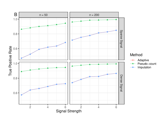
Refer to caption
Refer to caption
Fig. S1: Performance of LinDA with different zero-handling approaches (S6C0: 10-fold difference in library size, a binary covariate). Empirical false discovery rate (A) and true positive rates (B) were averaged over 100 simulation runs. The dashed horizontal line (A) indicates the target FDR level of 0.05. Note that the red and blue lines are overlapped as the covariate and sequencing depth are significantly correlated.
Refer to caption
Refer to caption
Fig. S2: Performance of LinDA with different zero-handling approaches (S0C0: log normal abundance distribution, a binary covariate). Empirical false discovery rate (A) and true positive rates (B) were averaged over 100 simulation runs. The dashed horizontal line (A) indicates the target FDR level of 0.05.
Refer to caption
Refer to caption
Fig. S3: Performance comparison between LinDA and MaAsLin2 (S0C0: log normal abundance distribution, a binary covariate). Empirical false discovery rate (A) and true positive rates (B) were averaged over 100 simulation runs. The dashed horizontal line (A) indicates the target FDR level of 0.05.
Refer to caption
Refer to caption
Fig. S4: Performance comparison (S0C1: log normal abundance distribution, a continuous covariate). Empirical false discovery rate (A) and true positive rates (B) were averaged over 100 simulation runs. Error bars (A) represent the 95% CIs of the method LinDA and the dashed horizontal line indicates the target FDR level of 0.05.
Refer to caption
Refer to caption
Fig. S5: Performance comparison (S0C2: log normal abundance distribution, a binary variable of interest and two confounders). Empirical false discovery rate (A) and true positive rates (B) were averaged over 100 simulation runs. Error bars (A) represent the 95% CIs of the method LinDA and the dashed horizontal line indicates the target FDR level of 0.05.
Refer to caption
Refer to caption
Fig. S6: Performance comparison (S1C0: zero inflated absolute abundances, a binary covariate). Empirical false discovery rate (A) and true positive rates (B) were averaged over 100 simulation runs. Error bars (A) represent the 95% CIs of the method LinDA and the dashed horizontal line indicates the target FDR level of 0.05.
Refer to caption
Refer to caption
Fig. S7: Performance comparison (S2C0: correlated absolute abundances, a binary covariate). Empirical false discovery rate (A) and true positive rates (B) were averaged over 100 simulation runs. Error bars (A) represent the 95% CIs of the method LinDA and the dashed horizontal line indicates the target FDR level of 0.05.
Refer to caption
Refer to caption
Fig. S8: Performance comparison (S4C0: smaller mπ‘šm, a binary covariate). Empirical false discovery rate (A) and true positive rates (B) were averaged over 1000 simulation runs. Error bars (A) represent the 95% CIs of the method LinDA and the dashed horizontal line indicates the target FDR level of 0.05.
Refer to caption
Refer to caption
Fig. S9: Performance comparison (S5C0: smaller n𝑛n, a binary covariate). Empirical false discovery rate (A) and true positive rates (B) were averaged over 100 simulation runs. Error bars (A) represent the 95% CIs of the method LinDA and the dashed horizontal line indicates the target FDR level of 0.05.
Refer to caption
Refer to caption
Fig. S10: Performance comparison (S6C0: 10-fold difference in library size, a binary covariate). Empirical false discovery rate (A) and true positive rates (B) were averaged over 100 simulation runs. Error bars (A) represent the 95% CIs of the method LinDA and the dashed horizontal line indicates the target FDR level of 0.05.
Refer to caption
Refer to caption
Fig. S11: Performance of ANCOM-BC disabling (ANCOM-BC-1) and enabling (ANCOM-BC-2) zero treatment (S6C0: 10-fold difference in library size, a binary covariate). Empirical false discovery rate (A) and true positive rates (B) were averaged over 100 simulation runs. The dashed horizontal line (A) indicates the target FDR level of 0.05.
Refer to caption
Refer to caption
Fig. S12: Performance comparison (S7C0: negative binomial abundance distribution, a binary covariate). Empirical false discovery rate (A) and true positive rates (B) were averaged over 100 simulation runs. Error bars (A) represent the 95% CIs of the method LinDA and the dashed horizontal line indicates the target FDR level of 0.05.
Refer to caption
Refer to caption
Fig. S13: Performance comparison (S8.1C0: pre-treatment and post-treatment comparison, a binary covariate). Empirical false discovery rate (A) and true positive rates (B) were averaged over 100 simulation runs. The dashed horizontal line (A) indicates the target FDR level of 0.05.
Refer to caption
Refer to caption
Fig. S14: Performance comparison (S8.2C0: replicate sampling, a binary covariate). Empirical false discovery rate (A) and true positive rates (B) were averaged over 100 simulation runs. The dashed horizontal line (A) indicates the target FDR level of 0.05.
Refer to caption
Refer to caption
Fig. S15: Performance comparison (S0C0 with strong compositional effects). Empirical false discovery rate (A) and true positive rates (B) were averaged over 100 simulation runs. Error bars (A) represent the 95% CIs of the method LinDA and the dashed horizontal line indicates the target FDR level of 0.05.

S2 Additional results of real data applications

Fig. S16–S19 show the effect size plots and volcano plots for the four datasets (CDI, IBD, RA, and SMOKE) respectively.
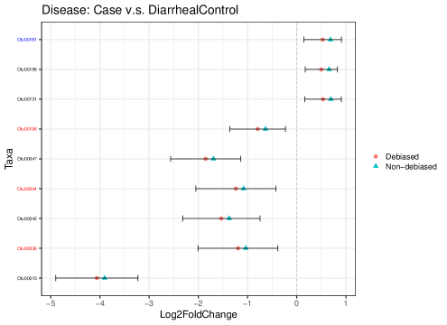
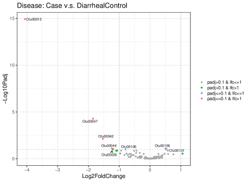
(a) A
Refer to caption
(b) B
Refer to caption
Fig. S16: Effect size plot (A) of differential taxa at FDR level of 0.1 and volcano plot (B) for the CDI dataset. The β€œDebiased” points represent the bias-corrected regression coefficients, and β€œNon-debiased” points represent the original (biased) regression coefficients. The error bars represent the 95% CIs of the β€œDebiased” points. The taxa in black are detected by LinDA, taxa in red are detected solely by LinDA, and the taxa in blue are missed by LinDA but detected by one or more of the other methods (A).
(a) A
Refer to caption
(b) B
Refer to caption
Fig. S17: Effect size plot (A) of differential taxa at FDR level of 0.1 and volcano plot (B) for the IBD dataset. The β€œDebiased” points represent the bias-corrected regression coefficients, and β€œNon-debiased” points represent the original (biased) regression coefficients. The error bars represent the 95% CIs of the β€œDebiased” points. The taxa in black are detected by LinDA, taxa in red are detected solely by LinDA, and taxa in blue are missed by LinDA but detected by two or more of the other methods (A).
(a) A
Refer to caption
(b) B
Refer to caption
Fig. S18: Effect size plot (A) of differential taxa at FDR level of 0.1 and volcano plot (B) for the RA dataset. The β€œDebiased” points represent the bias-corrected regression coefficients, and β€œNon-debiased” points represent the original (biased) regression coefficients. The error bars represent the 95% CIs of the β€œDebiased” points. The taxa in black are detected by LinDA, taxa in red are detected solely by LinDA, and taxa in blue are missed by LinDA but detected by two or more of the other methods (A).
(a) A
Refer to caption
(b) B
Refer to caption
Fig. S19: Effect size plot (A) of differential taxa detected by LinDA at FDR level of 0.1 and volcano plot (B) for the SMOKE dataset. The β€œDebiased” points represent the bias-corrected regression coefficients, and β€œNon-debiased” points represent the original (biased) regression coefficients. The error bars represent the 95% CIs of the β€œDebiased” points. The taxa in black are detected by LinDA, taxa in red are detected by LinDA but missed by MaAsLin2, and no taxa are detected by MaAsLin2 but missed by LinDA (A).

S3 Full comparisons of numerical studies
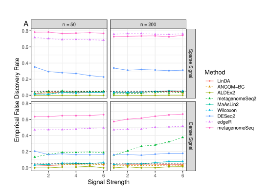
Fig. S20–S30 present the full result of all methods under different simulation settings.

Refer to caption
Refer to caption
Fig. S20: Full performance comparison (S0C0: log normal abundance distribution, a binary covariate). Empirical false discovery rate (A) and true positive rates (B) were averaged over 100 simulation runs. The dashed horizontal line (A) indicates the target FDR level of 0.05.
Refer to caption
Refer to caption
Fig. S21: Full performance comparison (S0C1: log normal abundance distribution, a continuous covariate). Empirical false discovery rate (A) and true positive rates (B) were averaged over 100 simulation runs. The dashed horizontal line (A) indicates the target FDR level of 0.05.
Refer to caption
Refer to caption
Fig. S22: Full performance comparison (S0C2: log normal abundance distribution, a binary variable of interest and two confounders). Empirical false discovery rate (A) and true positive rates (B) were averaged over 100 simulation runs. The dashed horizontal line (A) indicates the target FDR level of 0.05.
Refer to caption
Refer to caption
Fig. S23: Full performance comparison (S1C0: zero inflated absolute abundances, a binary covariate). Empirical false discovery rate (A) and true positive rates (B) were averaged over 100 simulation runs. The dashed horizontal line (A) indicates the target FDR level of 0.05.
Refer to caption
Refer to caption
Fig. S24: Full performance comparison (S2C0: correlated absolute abundances, a binary covariate). Empirical false discovery rate (A) and true positive rates (B) were averaged over 100 simulation runs. The dashed horizontal line (A) indicates the target FDR level of 0.05.
Refer to caption
Refer to caption
Fig. S25: Full performance comparison (S3C0: gamma abundance distribution, a binary covariate). Empirical false discovery rate (A) and true positive rates (B) were averaged over 100 simulation runs. The dashed horizontal line (A) indicates the target FDR level of 0.05.
Refer to caption
Refer to caption
Fig. S26: Full performance comparison (S4C0: smaller mπ‘šm, a binary covariate). Empirical false discovery rate (A) and true positive rates (B) were averaged over 1000 simulation runs. The dashed horizontal line (A) indicates the target FDR level of 0.05.
Refer to caption
Refer to caption
Fig. S27: Full performance comparison (S5C0: smaller n𝑛n, a binary covariate). Empirical false discovery rate (A) and true positive rates (B) were averaged over 100 simulation runs. The dashed horizontal line (A) indicates the target FDR level of 0.05.
Refer to caption
Refer to caption
Fig. S28: Full performance comparison (S6C0: 10-fold difference in library size, a binary covariate). Empirical false discovery rate (A) and true positive rates (B) were averaged over 100 simulation runs. The dashed horizontal line (A) indicates the target FDR level of 0.05.
Refer to caption
Refer to caption
Fig. S29: Full performance comparison (S7C0: negative binomial abundance distribution, a binary covariate). Empirical false discovery rate (A) and true positive rates (B) were averaged over 100 simulation runs. The dashed horizontal line (A) indicates the target FDR level of 0.05.
Refer to caption
Refer to caption
Fig. S30: Full performance comparison (S0C0 with strong compositional effects). Empirical false discovery rate (A) and true positive rates (B) were averaged over 100 simulation runs. The dashed horizontal line (A) indicates the target FDR level of 0.05.