ARA
Absolute Risk Aversion
VI
Variational Inference
VI-MPC
Variational Inference-Model Predictive Control
SOC
Stochastic Optimal Control
SVGD
Stein Variational Gradient Descent
SS
Stochastic Search
MPPI
Model Predictive Path Integral
MPC
Model Predictive Control
CEM
Cross Entropy Method
RL
Reinforcement Learning
KL
Kullback-Leibler
EM
Expectation Maximization
\externaldocument

paper/supplementary

Variational Inference MPC using Tsallis Divergence

Ziyi Wang12, Oswin So1, Jason Gibson, Bogdan Vlahov, Manan S. Gandhi
Guan-Horng Liu and Evangelos A. Theodorou
Autonomous Control and Decision Systems Lab
Georgia Institute of Technology, Atlanta, Georgia
1These authors contributed equally
2Correspondence to: ZiyiWang@gatech.edu
Abstract

In this paper, we provide a generalized framework for Variational Inference-Stochastic Optimal Control by using the non-extensive Tsallis divergence. By incorporating the deformed exponential function into the optimality likelihood function, a novel Tsallis Variational Inference-Model Predictive Control algorithm is derived, which includes prior works such as Variational Inference-Model Predictive Control, Model Predictive Path Integral Control, Cross Entropy Method, and Stein Variational Inference Model Predictive Control as special cases. The proposed algorithm allows for effective control of the cost/reward transform and is characterized by superior performance in terms of mean and variance reduction of the associated cost. The aforementioned features are supported by a theoretical and numerical analysis on the level of risk sensitivity of the proposed algorithm as well as simulation experiments on 5 different robotic systems with 3 different policy parameterizations.

I Introduction

Variational Inference (VI) is a powerful tool for approximating the posterior distribution of the unobserved random variables [1]. VI recasts the approximation problem as an optimization problem. Instead of directly approximating the target distribution p(z|x)𝑝conditional𝑧𝑥p(z|x) of the latent variable z𝑧z, VI minimizes the Kullback-Leibler (KL) divergence between a tractable variational distribution q(z)𝑞𝑧q(z) and the target distribution. Due to its faster convergence and comparable performance to Markov Chain Monte Carlo sampling methods, VI has received increasing attention in machine learning and robotics [2, 3, 4].

VI has been applied to Stochastic Optimal Control (SOC) problems recently. In Okada and Taniguchi [5], the authors formulated the SOC problem as a VI problem by setting the desired policy distribution as the target distribution. The VI-SOC framework works directly in the space of policy distributions instead of specific policy parameterizations in most SOC and Reinforcement Learning (RL) frameworks. This gives rise to a unified derivation for a variety of parametric policy distributions, such as unimodal Gaussian and Gaussian mixture in Okada and Taniguchi [5]. Lambert et al. [6] derived the VI-SOC algorithm for non-parametric policy distribution using Stein variational gradient descent. Apart from the policy distribution, the VI-SOC framework is characterized by two components, the optimality likelihood function and distributional distance metric. The optimality likelihood function measures the likelihood of trajectory samples to be optimal and defines the cost/reward transform to allow for different algorithmic developments. The distributional distance metric is the measure of distance between the variational distribution and target distribution.

In existing VI-SOC works, the KL divergence is used as the distributional distance metric due to its simplicity. On the other hand, recent advances in VI research involve extending the framework to other statistical divergences, such as the α𝛼\alpha-divergence [7] and χ𝜒\chi-divergence [8]. In Wang et al. [9], Regli and Silva [10], the authors proposed variants of the α𝛼\alpha-divergence to improve the performance and robustness of the inference algorithm. Wan et al. [11] further extended the VI framework to f𝑓f-divergence, which is a broad statistical divergence family that recovers the KL, α𝛼\alpha and χ𝜒\chi-divergence as special cases.

Tsallis divergence is another generalized divergence rooted in non-extensive statistical mechanics [12]. Tsallis divergence and Tsallis entropy are generalizations of the KL divergence and Shannon entropy respectively. The Tsallis entropy is non-additive (hence non-extensive) in the sense that for a system composed of (probabilistically) independent subsystems, the total entropy differs from the sum of the entropies of the subsystems [13]. Over the last two decades, an increasing number of complex natural, artificial and social systems have verified the predictions and consequences derived from the Tsallis entropy and divergence [14, 15, 16, 17]. Lee et al. [17] demonstrated that Tsallis entropy regularization leads to improved performance and faster convergence in RL applications.

In this paper, we provide a generalized formulation of the VI-SOC framework using the Tsallis divergence and introduce a novel Model Predictive Control (MPC) algorithm. The main contribution of our work is threefold:

  • We propose the Tsallis VI-MPC algorithm, which allows for additional control of the shape of the cost transform compared to previous VI-MPC algorithms using KL divergence.

  • We provide a holistic view of connections between Tsallis VI-SOC and the state-of-the-art Model Predictive Path Integral (MPPI) control, Cross Entropy Method (CEM) and Stochastic Search (SS) methods.

  • We show, both analytically and numerically, that the proposed Tsallis VI-SOC framework achieves lower cost variance than MPPI and CEM. We further demonstrate the superior performance of Tsallis VI-SOC in mean cost and variance minimization on simulated systems from control theory and robotics for 3 different choices of policy distributions.

The rest of this paper is organized as follows: in Section II, we review KL VI-SOC and derive the Tsallis VI-SOC framework. In Section III, we discuss the connections between Tsallis VI-SOC and related works. A reparameterization and analysis of the framework is included in Section IV, and we propose the novel Tsallis VI-MPC algorithm in Section V. We showcase the performance of the proposed algorithm against related works in Section VI and conclude the paper in Section VII.

II Tsallis Variational Inference-Stochastic Optimal Control

In this section, we review the VI-SOC formulation using KL divergence [5] and derive the novel Tsallis divergence VI-SOC framework.

II-A SOC Problem Formulation

In discrete time SOC, we work with trajectories τ{X,U}𝜏𝑋𝑈\tau\coloneqq\{X,U\} of state, X{x0,x1,,xT}nx×T+1𝑋subscript𝑥0subscript𝑥1subscript𝑥𝑇superscriptsubscript𝑛𝑥𝑇1X\coloneqq\{x_{0},x_{1},\dots,x_{T}\}\in\mathbb{R}^{n_{x}\times{T+1}}, and control, U{u0,u1,,uT1}nu×T𝑈subscript𝑢0subscript𝑢1subscript𝑢𝑇1superscriptsubscript𝑛𝑢𝑇U\coloneqq\{u_{0},u_{1},\dots,u_{T-1}\}\in\mathbb{R}^{n_{u}\times T} over a finite time horizon T>0𝑇0T>0. The goal in SOC problems is to minimize the expected cost defined by an arbitrary cost function J:nx×T×nu×T1+:𝐽superscriptsubscript𝑛𝑥𝑇superscriptsubscript𝑛𝑢𝑇1superscriptJ:\mathbb{R}^{n_{x}\times T}\times\mathbb{R}^{n_{u}\times T-1}\rightarrow\mathbb{R}^{+} with initial state distribution p(x0)𝑝subscript𝑥0p(x_{0}) and state transition probability p(xt+1|xt,ut)𝑝conditionalsubscript𝑥𝑡1subscript𝑥𝑡subscript𝑢𝑡p(x_{t+1}|x_{t},u_{t}) corresponding to stochastic dynamics xt+1=F(xt,ut,ϵt)subscript𝑥𝑡1𝐹subscript𝑥𝑡subscript𝑢𝑡subscriptitalic-ϵ𝑡x_{t+1}=F(x_{t},u_{t},\epsilon_{t}) where ϵtnϵsubscriptitalic-ϵ𝑡superscriptsubscript𝑛italic-ϵ\epsilon_{t}\in\mathbb{R}^{n_{\epsilon}} is the system stochasticity.

II-B KL VI-SOC

We can formulate the SOC problem as an inference problem and apply methods from VI. To apply VI to SOC, we introduce a dummy optimality variable o{0,1}𝑜01o\in\{0,1\} with o=1𝑜1o=1 indicating that the trajectory τ={X,U}𝜏𝑋𝑈\tau=\{X,U\} is optimal. Table I compares the differences in notation between conventional VI methods and SOC formulated as a VI problem.

The objective of VI-SOC is to sample from the posterior distribution

p(τ|o)=p(o=1|τ)p(τ)p(o)=p(o=1|τ)p(o=1)p(x0)t=0T1p(xt+1|xt,ut)p(ut).𝑝conditional𝜏𝑜𝑝𝑜conditional1𝜏𝑝𝜏𝑝𝑜𝑝𝑜conditional1𝜏𝑝𝑜1𝑝subscript𝑥0superscriptsubscriptproduct𝑡0𝑇1𝑝conditionalsubscript𝑥𝑡1subscript𝑥𝑡subscript𝑢𝑡𝑝subscript𝑢𝑡\begin{split}p(\tau|o)&=\frac{p(o=1|\tau)p(\tau)}{p(o)}\\ &=\frac{p(o=1|\tau)}{p(o=1)}p(x_{0})\prod_{t=0}^{T-1}p(x_{t+1}|x_{t},u_{t})p(u_{t}).\end{split} (1)

Here p(xt+1|xt,ut)𝑝conditionalsubscript𝑥𝑡1subscript𝑥𝑡subscript𝑢𝑡p(x_{t+1}|x_{t},u_{t}) is the state transition probability, p(x0)𝑝subscript𝑥0p(x_{0}) is the initial state distribution and p(ut)𝑝subscript𝑢𝑡p(u_{t}) is some prior control distribution (e.g. zero mean Gaussian or uniform distribution). For simplicity, we use o𝑜o to indicate o=1𝑜1o=1 and osuperscript𝑜o^{\prime} for o=0𝑜0o=0 from here on. We can now formulate the VI-SOC objective as minimizing the distance between a controlled distribution q(τ)𝑞𝜏q(\tau) and the target distribution p(τ|o)𝑝conditional𝜏𝑜p(\tau|o)

q(τ)=argminq(τ)𝒟KL(q(τ)p(τ|o))=argminq(τ)𝔼q(τ)[logp(X|U)q(U)p(o|τ)p(o)p(X|U)p(U)]=argminq(τ)𝔼q(τ)[logp(o|τ)+t=0T1logq(ut)p(ut)],\begin{split}q^{*}(\tau)&=\operatorname*{arg\,min}_{q(\tau)}\mathcal{D}_{KL}\left({q(\tau)}\parallel{p(\tau|o)}\right)\\ &=\operatorname*{arg\,min}_{q(\tau)}\mathbb{E}_{q(\tau)}\Bigg{[}\log\frac{p(X|U)q(U)}{\frac{p(o|\tau)}{p(o)}p(X|U)p(U)}\Bigg{]}\\ &=\operatorname*{arg\,min}_{q(\tau)}\mathbb{E}_{q(\tau)}\Bigg{[}-\log p(o|\tau)+\sum_{t=0}^{T-1}\log\frac{q(u_{t})}{p(u_{t})}\Bigg{]},\end{split} (2)

where the constant p(o)𝑝𝑜p(o) is dropped. The first term in the objective measures the likelihood of a trajectory being optimal while the second term serves as regularization. Splitting the expectation in the first term, we get

q(U)=argminq(U){𝔼q(U)[𝔼p(X|U)[logp(o|τ)]]+𝒟KL(q(U)p(U))},superscript𝑞𝑈subscriptargmin𝑞𝑈subscript𝔼𝑞𝑈delimited-[]subscript𝔼𝑝conditional𝑋𝑈delimited-[]𝑝|𝑜𝜏subscript𝒟𝐾𝐿parallel-to𝑞𝑈𝑝𝑈\begin{split}q^{*}(U)=\operatorname*{arg\,min}_{q(U)}&\Big{\{}-\mathbb{E}_{q(U)}[\mathbb{E}_{p{(X|U)}}[\log p(o|\tau)]]\\ &+\mathcal{D}_{KL}\left({q(U)}\parallel{p(U)}\right)\Big{\}},\end{split} (3)

where p(U)𝑝𝑈p(U) and q(U)𝑞𝑈q(U) represent t=0T1p(ut)superscriptsubscriptproduct𝑡0𝑇1𝑝subscript𝑢𝑡\prod_{t=0}^{T-1}p(u_{t}) and t=0T1q(ut)superscriptsubscriptproduct𝑡0𝑇1𝑞subscript𝑢𝑡\prod_{t=0}^{T-1}q(u_{t}) respectively due to independence and p(X|U)=p(x0)t=0T1p(xt+1|xt,ut)𝑝conditional𝑋𝑈𝑝subscript𝑥0superscriptsubscriptproduct𝑡0𝑇1𝑝conditionalsubscript𝑥𝑡1subscript𝑥𝑡subscript𝑢𝑡p(X|U)=p(x_{0})\prod_{t=0}^{T-1}p(x_{t+1}|x_{t},u_{t}).

Optimality Likelihood: The optimality likelihood in Eq. 3 can be parameterized by a non-increasing function of the trajectory cost J(X,U)𝐽𝑋𝑈J(X,U) as p(o|τ)f(J(X,U))𝑝conditional𝑜𝜏𝑓𝐽𝑋𝑈p(o|\tau)\coloneqq f(J(X,U)). The monotonicity requirement ensures that trajectories incurring higher costs are always less likely to be optimal. Common choices of f𝑓f include f(x)=exp(x)𝑓𝑥𝑥f(x)=\exp(-x) and f(x)=𝟏{xγ}𝑓𝑥subscript1𝑥𝛾f(x)=\bm{1}_{\{x\leq\gamma\}}. In this paper, we choose f(x)=exp(x)𝑓𝑥𝑥f(x)=\exp(-x) such that logp(o|τ)=J(X,U)𝑝conditional𝑜𝜏𝐽𝑋𝑈\log p(o|\tau)=-J(X,U). To avoid excessive notation, we abuse the notation to define J(U)𝔼p(X|U)[J(X,U)]𝐽𝑈subscript𝔼𝑝conditional𝑋𝑈delimited-[]𝐽𝑋𝑈J(U)\coloneqq\mathbb{E}_{p(X|U)}[J(X,U)] and the N𝑁N-sample empirical approximation of the expectation J=n=1N[J(n)]𝐽superscriptsubscript𝑛1𝑁delimited-[]superscript𝐽𝑛J=\sum_{n=1}^{N}[J^{(n)}]. Hence, Eq. 3 takes the form

q(U)=argminq(U)𝔼q(U)[J(X,U)]+𝒟KL(q(U)p(U)),superscript𝑞𝑈subscriptargmin𝑞𝑈subscript𝔼𝑞𝑈delimited-[]𝐽𝑋𝑈subscript𝒟𝐾𝐿conditional𝑞𝑈𝑝𝑈q^{*}(U)=\operatorname*{arg\,min}_{q(U)}\mathbb{E}_{q(U)}[J(X,U)]+\mathcal{D}_{KL}\left({q(U)}\parallel{p(U)}\right), (4)

which can be interpreted as an application of the famous maximum entropy principle.

TABLE I: Notation comparison between Variational Inference and Variational Inference-Stochastic Optimal Control.
VI VI-SOC
Notation Meaning Notation Meaning
x𝑥x data o𝑜o optimality
z𝑧z latent variable τ𝜏\tau trajectory
p(z)𝑝𝑧p(z) prior distribution p(τ)𝑝𝜏p(\tau) prior distribution
q(z)𝑞𝑧q(z) variational distribution q(τ)𝑞𝜏q(\tau) controlled distribution
p(x|z)𝑝conditional𝑥𝑧p(x|z) generative model p(o|τ)𝑝conditional𝑜𝜏p(o|\tau) optimality likelihood
p(z|x)𝑝conditional𝑧𝑥p(z|x) posterior distribution p(τ|o)𝑝conditional𝜏𝑜p(\tau|o) optimal distribution

II-C Tsallis VI-SOC

In this subsection, we use the Tsallis divergence as the regularization function and derive the Tsallis-VI-SOC algorithm. First, we define the deformed logarithm and exponential as

logr(x)subscript𝑟𝑥\displaystyle\log_{r}(x) =xr11r1,absentsuperscript𝑥𝑟11𝑟1\displaystyle=\frac{x^{r-1}-1}{r-1}, (5)
expr(x)subscript𝑟𝑥\displaystyle\exp_{r}(x) =(1+(r1)x)+1r1,absentsuperscriptsubscript1𝑟1𝑥1𝑟1\displaystyle=(1+(r-1)x)_{+}^{\frac{1}{r-1}}, (6)

where ()+max(0,)subscript0(\cdot)_{+}\coloneqq\max(0,\cdot) and r>0𝑟0r>0. Using logrsubscript𝑟\log_{r} and exprsubscript𝑟\exp_{r} we can define the Tsallis entropy and the corresponding Tsallis divergence [12] as

𝒮r(q(z))𝔼q[logrq(z)]=1r1(q(z)rdz1),subscript𝒮𝑟𝑞𝑧subscript𝔼𝑞delimited-[]subscript𝑟𝑞𝑧1𝑟1𝑞superscript𝑧𝑟d𝑧1\begin{split}\mathcal{S}_{r}(q(z))\coloneqq&-\mathbb{E}_{q}[\log_{r}q(z)]\\ =&-\frac{1}{r-1}\left(\int q(z)^{r}{\textnormal{d}}z-1\right),\end{split} (7)

and

𝒟r(q(z)p(z))𝔼q[logrq(z)p(z)]=1r1(q(z)(q(z)p(z))r1dz1).subscript𝒟𝑟conditional𝑞𝑧𝑝𝑧subscript𝔼𝑞delimited-[]subscript𝑟𝑞𝑧𝑝𝑧1𝑟1𝑞𝑧superscript𝑞𝑧𝑝𝑧𝑟1d𝑧1\begin{split}\mathcal{D}_{r}\left({q(z)}\parallel{p(z)}\right)\coloneqq&\mathbb{E}_{q}\left[\log_{r}\frac{q(z)}{p(z)}\right]\\ =&\frac{1}{r-1}\left(\int q(z)\left(\frac{q(z)}{p(z)}\right)^{r-1}{\textnormal{d}}z-1\right).\end{split} (8)

Note that as r1𝑟1r\rightarrow 1, logrlogsubscript𝑟\log_{r}\rightarrow\log, exprexpsubscript𝑟\exp_{r}\rightarrow\exp, 𝒟r𝒟KLsubscript𝒟𝑟subscript𝒟𝐾𝐿\mathcal{D}_{r}\rightarrow\mathcal{D}_{KL} and 𝒮r𝒮subscript𝒮𝑟𝒮\mathcal{S}_{r}\rightarrow\mathcal{S}, where 𝒮𝒮\mathcal{S} is the Shannon entropy, recovering the KL VI-SOC framework.

Versions of Tsallis Statistics: In our definition of the deformed logarithm and exponential in Eqs. 5 and 6, we use the variable r𝑟r instead of the q𝑞q used in most literature to avoid assigning multiple meanings to q𝑞q. Also, our definition of logrsubscript𝑟\log_{r} and exprsubscript𝑟\exp_{r} differ from its original definitions [18], but the original can be recovered with r=2rsuperscript𝑟2𝑟r^{\prime}=2-r, where rsuperscript𝑟r^{\prime} corresponding to the value used in [18]. Additionally, there are multiple formulations of the Tsallis entropy differing in their definitions of the internal energy and how expectations are taken [12, 19, 20]. We have chosen to use the formulation from [12] due to its simplicity in computing the expectation. However, as shown in [21], they are equivalent and can be recovered from each other via a change of variables.

We can now define a new objective by replacing the KL divergence regularizer in Eq. 4 with the Tsallis divergence and introducing a parameter λ𝜆\lambda that multiplies the optimality likelihood to make the regularization strength tunable:

q(U)=argminq(U)λ1𝔼q(U)[J]+𝒟r(q(U)p(U)).superscript𝑞𝑈subscriptargmin𝑞𝑈superscript𝜆1subscript𝔼𝑞𝑈delimited-[]𝐽subscript𝒟𝑟conditional𝑞𝑈𝑝𝑈q^{*}(U)=\operatorname*{arg\,min}_{q(U)}\lambda^{-1}\mathbb{E}_{q(U)}[J]+\mathcal{D}_{r}\left({q(U)}\parallel{p(U)}\right). (9)

The controlled distribution has to satisfy the additional constraint of q(U)dU=1𝑞𝑈d𝑈1\int q(U)\,{\textnormal{d}}U=1. The optimal policy distribution qsuperscript𝑞q^{*} can be explicitly solved for with the form

q(U)=expr(λ~1J)p(U)expr(λ~1J)p(U)dU,superscript𝑞𝑈subscript𝑟superscript~𝜆1𝐽𝑝𝑈subscript𝑟superscript~𝜆1𝐽𝑝𝑈d𝑈q^{*}(U)=\frac{\exp_{r}\left(-\tilde{\lambda}^{-1}J\right)p(U)}{\int\exp_{r}\left(-\tilde{\lambda}^{-1}J\right)p(U)\,{\textnormal{d}}U}, (10)

where λ~=α(r1)λ~𝜆𝛼𝑟1𝜆\tilde{\lambda}=\alpha(r-1)\lambda with α𝛼\alpha being the Lagrange multiplier for the constraint that qsuperscript𝑞q^{*} integrates to 111. A detailed derivation can be found in Section SM-1 of the supplementary materials. We can now use Eq. 10 to obtain the optimal control distribution by transforming the prior distribution.

II-D Update Laws

In general, it is computationally inefficient to sample from q(U)superscript𝑞𝑈q^{*}(U) via Eq. 10 directly. Instead, we can approximate q(U)superscript𝑞𝑈q^{*}(U) by some policy π(U)𝜋𝑈\pi(U) lying in a class ΠΠ\Pi of tractable distributions and solve for an iterative update law by minimizing the KL divergence between π(U)𝜋𝑈\pi(U) and q(U)superscript𝑞𝑈q^{*}(U):

πk+1(U)=argminπ(U)Π𝒟KL(q(U)π(U)).superscript𝜋𝑘1𝑈subscriptargmin𝜋𝑈Πsubscript𝒟𝐾𝐿conditionalsuperscript𝑞𝑈𝜋𝑈\pi^{k+1}(U)=\operatorname*{arg\,min}_{\pi(U)\in\Pi}\mathcal{D}_{KL}\left({q^{*}(U)}\parallel{\pi(U)}\right). (11)

However, because one can only evaluate q(U)superscript𝑞𝑈q^{*}(U) at a finite number of points {U(n)}n=1Nsuperscriptsubscriptsuperscript𝑈𝑛𝑛1𝑁\{U^{(n)}\}_{n=1}^{N}, we instead approximate q(U)superscript𝑞𝑈q^{*}(U) by the empirical distribution q~(U)superscript~𝑞𝑈\tilde{q}^{*}(U) with weights w(n)superscript𝑤𝑛w^{(n)}:

q~(U)=n=1Nw(n)𝟏{U=U(n)},superscript~𝑞𝑈superscriptsubscript𝑛1𝑁superscript𝑤𝑛subscript1𝑈superscript𝑈𝑛\displaystyle\tilde{q}^{*}(U)=\sum_{n=1}^{N}w^{(n)}\bm{1}_{\{U=U^{(n)}\}}, (12)
w(n)=q(U(n))n=1Nq(U(n)).superscript𝑤𝑛superscript𝑞superscript𝑈𝑛superscriptsubscriptsuperscript𝑛1𝑁superscript𝑞superscript𝑈superscript𝑛\displaystyle w^{(n)}=\frac{q^{*}(U^{(n)})}{\sum_{n^{\prime}=1}^{N}q^{*}(U^{(n^{\prime})})}. (13)

We now solve Eq. 11 for 3 different policy classes: unimodal Gaussian, Gaussian mixture and a nonparametric policy corresponding to Stein Variational Gradient Descent (SVGD) [6, 22]. The full derivations for each can be found in the supplementary material in Section SM-2.

Unimodal Gaussian: For a unimodal Gaussian policy distribution with parameters Θ{(μt,Σt)}t=0T1Θsuperscriptsubscriptsubscript𝜇𝑡subscriptΣ𝑡𝑡0𝑇1\Theta\coloneqq\{(\mu_{t},\Sigma_{t})\}_{t=0}^{T-1}, the update laws for the k+1𝑘1k+1th iteration take the form of

μtk+1subscriptsuperscript𝜇𝑘1𝑡\displaystyle\mu^{k+1}_{t} =n=1Nw(n)ut(n),absentsuperscriptsubscript𝑛1𝑁superscript𝑤𝑛superscriptsubscript𝑢𝑡𝑛\displaystyle=\sum_{n=1}^{N}w^{(n)}u_{t}^{(n)}, (14)
Σtk+1subscriptsuperscriptΣ𝑘1𝑡\displaystyle\Sigma^{k+1}_{t} =n=1Nw(n)(ut(n)μtk+1)(ut(n)μtk+1)T.absentsuperscriptsubscript𝑛1𝑁superscript𝑤𝑛superscriptsubscript𝑢𝑡𝑛superscriptsubscript𝜇𝑡𝑘1superscriptsuperscriptsubscript𝑢𝑡𝑛superscriptsubscript𝜇𝑡𝑘1T\displaystyle=\sum_{n=1}^{N}w^{(n)}(u_{t}^{(n)}-\mu_{t}^{k+1})(u_{t}^{(n)}-\mu_{t}^{k+1})^{\mathrm{T}}. (15)

Gaussian Mixture: Alternatively, the policy distribution can be an L𝐿L-mode mixture of Gaussian distribution with parameters Θ{θl}l=1LΘsuperscriptsubscriptsubscript𝜃𝑙𝑙1𝐿\Theta\coloneqq\{\theta_{l}\}_{l=1}^{L} for θl(ϕl,{μl,t,Σl,t}t=0T1)subscript𝜃𝑙subscriptitalic-ϕ𝑙superscriptsubscriptsubscript𝜇𝑙𝑡subscriptΣ𝑙𝑡𝑡0𝑇1\theta_{l}\coloneqq(\phi_{l},\{\mu_{l,t},\Sigma_{l,t}\}_{t=0}^{T-1}), where ϕlsubscriptitalic-ϕ𝑙\phi_{l} is the mixture weight for the l𝑙lth component. Although it is not possible to directly solve Eq. 11 in this case, we draw from Expectation Maximization (EM) to derive an iterative update scheme for the k+1𝑘1k+1th iteration with the form

ϕlk+1superscriptsubscriptitalic-ϕ𝑙𝑘1\displaystyle\phi_{l}^{k+1} =Nll=1LNl,absentsubscript𝑁𝑙superscriptsubscriptsuperscript𝑙1𝐿subscript𝑁superscript𝑙\displaystyle=\frac{N_{l}}{\sum_{l^{\prime}=1}^{L}N_{l^{\prime}}}, (16)
μl,tk+1superscriptsubscript𝜇𝑙𝑡𝑘1\displaystyle\mu_{l,t}^{k+1} =1Nln=1Nηl(utn)w(n)utn,absent1subscript𝑁𝑙superscriptsubscript𝑛1𝑁subscript𝜂𝑙superscriptsubscript𝑢𝑡𝑛superscript𝑤𝑛superscriptsubscript𝑢𝑡𝑛\displaystyle=\frac{1}{N_{l}}\sum_{n=1}^{N}\eta_{l}(u_{t}^{n})w^{(n)}u_{t}^{n}, (17)
Σl,tk+1superscriptsubscriptΣ𝑙𝑡𝑘1\displaystyle\Sigma_{l,t}^{k+1} =1Nln=1Nηl(utn)w(n)(utnμl,tk+1)(utnμl,tk+1)T,absent1subscript𝑁𝑙superscriptsubscript𝑛1𝑁subscript𝜂𝑙superscriptsubscript𝑢𝑡𝑛superscript𝑤𝑛subscriptsuperscript𝑢𝑛𝑡superscriptsubscript𝜇𝑙𝑡𝑘1superscriptsubscriptsuperscript𝑢𝑛𝑡superscriptsubscript𝜇𝑙𝑡𝑘1T\displaystyle=\frac{1}{N_{l}}\sum_{n=1}^{N}\eta_{l}(u_{t}^{n})w^{(n)}(u^{n}_{t}-\mu_{l,t}^{k+1})(u^{n}_{t}-\mu_{l,t}^{k+1})^{\mathrm{T}}, (18)

where

ηl(ut(n))subscript𝜂𝑙superscriptsubscript𝑢𝑡𝑛\displaystyle\eta_{l}(u_{t}^{(n)}) =ϕlk𝒩(ut(n)|μl,tk,Σl,tk)l=1Lϕlk𝒩(ut(n)|μl,tk,Σl,tk),absentsuperscriptsubscriptitalic-ϕ𝑙𝑘𝒩conditionalsuperscriptsubscript𝑢𝑡𝑛superscriptsubscript𝜇𝑙𝑡𝑘superscriptsubscriptΣ𝑙𝑡𝑘superscriptsubscriptsuperscript𝑙1𝐿superscriptsubscriptitalic-ϕsuperscript𝑙𝑘𝒩conditionalsuperscriptsubscript𝑢𝑡𝑛superscriptsubscript𝜇superscript𝑙𝑡𝑘superscriptsubscriptΣsuperscript𝑙𝑡𝑘\displaystyle=\frac{\phi_{l}^{k}{\mathcal{N}}(u_{t}^{(n)}|\mu_{l,t}^{k},\Sigma_{l,t}^{k})}{\sum_{l^{\prime}=1}^{L}\phi_{l^{\prime}}^{k}{\mathcal{N}}(u_{t}^{(n)}|\mu_{l^{\prime},t}^{k},\Sigma_{l^{\prime},t}^{k})}, (19)
Nlsubscript𝑁𝑙\displaystyle N_{l} =n=1Nt=0T1ηl(ut(n))w(n).absentsuperscriptsubscript𝑛1𝑁superscriptsubscript𝑡0𝑇1subscript𝜂𝑙superscriptsubscript𝑢𝑡𝑛superscript𝑤𝑛\displaystyle=\sum_{n=1}^{N}\sum_{t=0}^{T-1}\eta_{l}(u_{t}^{(n)})w^{(n)}. (20)

Stein Variational Policy: The policy can also be a non-parametric distribution approximated by a set of particles Θ{θl}l=1LΘsuperscriptsubscriptsubscript𝜃𝑙𝑙1𝐿\Theta\coloneqq\{\theta_{l}\}_{l=1}^{L} for some parametrized policy π^(U;θ)^𝜋𝑈𝜃\hat{\pi}(U;\theta). In [6], π^^𝜋\hat{\pi} is taken to be a unimodal Gaussian with fixed variance, where θnx×(T1)𝜃superscriptsubscript𝑛𝑥𝑇1\theta\in\mathbb{R}^{n_{x}\times(T-1)} corresponds to the mean. The update law of each Stein particle for the k+1𝑘1k+1th iteration has the form

θlk+1superscriptsubscript𝜃𝑙𝑘1\displaystyle\theta_{l}^{k+1} =θlk+ϵϕ^(θlk),absentsuperscriptsubscript𝜃𝑙𝑘italic-ϵsuperscript^italic-ϕsuperscriptsubscript𝜃𝑙𝑘\displaystyle=\theta_{l}^{k}+\epsilon\hat{\phi}^{*}(\theta_{l}^{k}), (21)
ϕ^(θ)superscript^italic-ϕ𝜃\displaystyle\hat{\phi}^{*}(\theta) =l=1Lk^(θl,θ)G(θm)+θlk^(θl,θ),absentsuperscriptsubscript𝑙1𝐿^𝑘subscript𝜃𝑙𝜃𝐺subscript𝜃𝑚subscriptsubscript𝜃𝑙^𝑘subscript𝜃𝑙𝜃\displaystyle=\sum_{l=1}^{L}\hat{k}(\theta_{l},\theta)G(\theta_{m})+\nabla_{\theta_{l}}\hat{k}(\theta_{l},\theta), (22)
G(θl)𝐺subscript𝜃𝑙\displaystyle G(\theta_{l}) =s=1Sw(l,s)θlogπ^(U(n),θl)s=1Sw(l,s),absentsuperscriptsubscript𝑠1𝑆superscript𝑤𝑙𝑠subscript𝜃^𝜋superscript𝑈𝑛subscript𝜃𝑙superscriptsubscript𝑠1𝑆superscript𝑤𝑙𝑠\displaystyle=\frac{\sum_{s=1}^{S}w^{(l,s)}\nabla_{\theta}\log\hat{\pi}(U^{(n)},\theta_{l})}{\sum_{s=1}^{S}w^{(l,s)}}, (23)

where the N𝑁N is chosen such that N=LS𝑁𝐿𝑆N=LS, k^^𝑘\hat{k} is a kernel function, and w(l,s)=w(m+L(l1))superscript𝑤𝑙𝑠superscript𝑤𝑚𝐿𝑙1w^{(l,s)}=w^{(m+L(l-1))}, where S𝑆S denotes the number of rollouts for each of the L𝐿L particle. As noted in [23], SVGD becomes less effective as the dimensionality of the particles increases due to the inverse relationship between the repulsion force in the update law and the dimensionality. Hence, we follow [6] in choosing a sum of local kernel functions as our choice of k^^𝑘\hat{k}.

TABLE II: Comparison of the objective and the update law for a unimodal Gaussian policy with fixed variance between different SOC approaches.
Formulation Objective (Minimize) Update Law for Unimodal Gaussian
Tsallis VI-SOC λ𝔼[logp(o|τ)]+𝒟r(qp)𝜆𝔼delimited-[]𝑝conditional𝑜𝜏subscript𝒟𝑟conditional𝑞𝑝-\lambda\mathbb{E}[\log p(o|\tau)]+\mathcal{D}_{r}\left({q}\parallel{p}\right) θtk+1=n=1Nexpr(λ~1Jn)s(utn)utnn=1Nexpr(λ~1Jn)s(utn)superscriptsubscript𝜃𝑡𝑘1superscriptsubscript𝑛1𝑁subscript𝑟superscript~𝜆1superscript𝐽𝑛𝑠subscriptsuperscript𝑢𝑛𝑡subscriptsuperscript𝑢𝑛𝑡superscriptsubscriptsuperscript𝑛1𝑁subscript𝑟superscript~𝜆1superscript𝐽superscript𝑛𝑠subscriptsuperscript𝑢superscript𝑛𝑡\theta_{t}^{k+1}=\sum_{n=1}^{N}\frac{\exp_{r}\left(-\tilde{\lambda}^{-1}J^{n}\right)s(u^{n}_{t})u^{n}_{t}}{\sum_{n^{\prime}=1}^{N}\exp_{r}\left(-\tilde{\lambda}^{-1}J^{n^{\prime}}\right)s(u^{n^{\prime}}_{t})}
KL VI-SOC λ𝔼[logp(o|τ)]+𝒟KL(qp)𝜆𝔼delimited-[]𝑝conditional𝑜𝜏subscript𝒟𝐾𝐿conditional𝑞𝑝-\lambda\mathbb{E}[\log p(o|\tau)]+\mathcal{D}_{KL}\left({q}\parallel{p}\right) θtk+1=n=1Nexp(λ1Jn)s(utn)utnn=1Nexp(λ1Jn)s(utn)superscriptsubscript𝜃𝑡𝑘1superscriptsubscript𝑛1𝑁superscript𝜆1superscript𝐽𝑛𝑠subscriptsuperscript𝑢𝑛𝑡subscriptsuperscript𝑢𝑛𝑡superscriptsubscriptsuperscript𝑛1𝑁superscript𝜆1superscript𝐽superscript𝑛𝑠subscriptsuperscript𝑢superscript𝑛𝑡\theta_{t}^{k+1}=\sum_{n=1}^{N}\frac{\exp\left(-\lambda^{-1}J^{n}\right)s(u^{n}_{t})u^{n}_{t}}{\sum_{n^{\prime}=1}^{N}\exp\left(-\lambda^{-1}J^{n^{\prime}}\right)s(u^{n^{\prime}}_{t})}
SS-SOC 𝔼[S(J)]𝔼delimited-[]𝑆𝐽\mathbb{E}[S(J)] θtk+1=θtk+βn=1NS(Jn)(utn1Nn~=1Nutn~)n=1NS(Jn)utnsuperscriptsubscript𝜃𝑡𝑘1superscriptsubscript𝜃𝑡𝑘𝛽superscriptsubscript𝑛1𝑁𝑆superscript𝐽𝑛superscriptsubscript𝑢𝑡𝑛1𝑁superscriptsubscript~𝑛1𝑁superscriptsubscript𝑢𝑡~𝑛superscriptsubscriptsuperscript𝑛1𝑁𝑆superscript𝐽superscript𝑛superscriptsubscript𝑢𝑡superscript𝑛\theta_{t}^{k+1}=\theta_{t}^{k}+\beta\sum_{n=1}^{N}\frac{S(J^{n})(u_{t}^{n}-\frac{1}{N}\sum_{\tilde{n}=1}^{N}u_{t}^{\tilde{n}})}{\sum_{n^{\prime}=1}^{N}S(J^{n^{\prime}})u_{t}^{n^{\prime}}}
MPPI 𝔼[J]+𝒟KL(qp)𝔼delimited-[]𝐽subscript𝒟𝐾𝐿conditional𝑞𝑝\mathbb{E}[J]+\mathcal{D}_{KL}\left({q}\parallel{p}\right) θtk+1=θtk+n=1Nexp(λ1Jn)s(utn)utnn=1Nexp(λ1Jn)s(utn)superscriptsubscript𝜃𝑡𝑘1superscriptsubscript𝜃𝑡𝑘superscriptsubscript𝑛1𝑁superscript𝜆1superscript𝐽𝑛𝑠superscriptsubscript𝑢𝑡𝑛superscriptsubscript𝑢𝑡𝑛superscriptsubscriptsuperscript𝑛1𝑁superscript𝜆1superscript𝐽superscript𝑛𝑠superscriptsubscript𝑢𝑡superscript𝑛\theta_{t}^{k+1}=\theta_{t}^{k}+\sum_{n=1}^{N}\frac{\exp(-\lambda^{-1}J^{n})s(u_{t}^{n})u_{t}^{n}}{\sum_{n^{\prime}=1}^{N}\exp(-\lambda^{-1}J^{n^{\prime}})s(u_{t}^{n^{\prime}})}
CEM 𝔼[J]𝔼delimited-[]𝐽\mathbb{E}[J] θtk+1=αθtk+(1α)n=1N𝟏{Jnγ}utnn=1N𝟏{Jnγ}superscriptsubscript𝜃𝑡𝑘1𝛼superscriptsubscript𝜃𝑡𝑘1𝛼superscriptsubscript𝑛1𝑁subscript1superscript𝐽𝑛𝛾superscriptsubscript𝑢𝑡𝑛superscriptsubscriptsuperscript𝑛1𝑁subscript1superscript𝐽superscript𝑛𝛾\theta_{t}^{k+1}=\alpha\theta_{t}^{k}+(1-\alpha)\sum_{n=1}^{N}\frac{\bm{1}_{\{J^{n}\leq\gamma\}}u_{t}^{n}}{\sum_{n^{\prime}=1}^{N}\bm{1}_{\{J^{n^{\prime}}\leq\gamma\}}}

III Connections to Related Works

In this section, we compare VI-SOC with three sampling-based methods from optimization, thermodynamics, and information theory that have been applied to stochastic control problems. A comparison of problem formulations and update laws for different approaches with a unimodal Gaussian policy is in Table II.

III-A Stochastic Search

SS [24] is a stochastic optimization scheme and has also been applied to the SOC setting [25, 26]. SS-SOC parameterizes the control policy with a distribution from the exponential family during problem formulation and optimizes with respect to policy parameters whereas VI-SOC performs optimization at the distribution level. The SS-SOC framework formulates the problem as

θ=argmaxθ𝔼π(U;θ)[S(𝔼p(X|U)[J(X,U)])],superscript𝜃subscriptargmax𝜃subscript𝔼𝜋𝑈𝜃delimited-[]𝑆subscript𝔼𝑝conditional𝑋𝑈delimited-[]𝐽𝑋𝑈\theta^{*}=\operatorname*{arg\,max}_{\theta}\mathbb{E}_{\pi(U;\theta)}\left[S(\mathbb{E}_{p(X|U)}[J(X,U)])\right], (24)

where S()𝑆S(\cdot) is a monotonically decreasing shape function. Note that in Eq. 24, the expectation taken with respect to p(X|U)𝑝conditional𝑋𝑈p(X|U) is inside the shape function S𝑆S as opposed to outside as in Eq. 3. For convex shape/optimality likelihood functions, the objective in VI-SOC corresponds to an upper bound of that in SS-SOC, i.e.,

S(𝔼p(X|U)[J(X,U)])𝔼p(X|U)[S(J(X,U))].𝑆subscript𝔼𝑝conditional𝑋𝑈delimited-[]𝐽𝑋𝑈subscript𝔼𝑝conditional𝑋𝑈delimited-[]𝑆𝐽𝑋𝑈S(\mathbb{E}_{p(X|U)}[J(X,U)])\leq\mathbb{E}_{p(X|U)}[S(J(X,U))]. (25)

A detailed comparison of the two formulations can be found in [5].

The parameter update of SS-SOC has the form

θtk+1=θtk+βn=1NS(J(n))(T(ut(n))1Nn~=1NT(ut(n~)))n=1NS(J(n)),superscriptsubscript𝜃𝑡𝑘1superscriptsubscript𝜃𝑡𝑘𝛽superscriptsubscript𝑛1𝑁𝑆superscript𝐽𝑛𝑇superscriptsubscript𝑢𝑡𝑛1𝑁superscriptsubscript~𝑛1𝑁𝑇subscriptsuperscript𝑢~𝑛𝑡superscriptsubscriptsuperscript𝑛1𝑁𝑆superscript𝐽superscript𝑛\theta_{t}^{k+1}=\theta_{t}^{k}+\beta\sum_{n=1}^{N}\frac{S(J^{(n)})(T(u_{t}^{(n)})-\frac{1}{N}\sum_{\tilde{n}=1}^{N}T(u^{(\tilde{n})}_{t}))}{\sum_{n^{\prime}=1}^{N}S(J^{(n^{\prime})})}, (26)

where T()𝑇T(\cdot) denotes the sufficient statistic for the corresponding parameter and β𝛽\beta is the step size. In the case of a unimodal Gaussian policy, the update in Eq. 26 is equivalent to Eqs. 14 and 15 with S(J)=expr(λ~1J)𝑆𝐽subscript𝑟superscript~𝜆1𝐽S(J)=\exp_{r}(-\tilde{\lambda}^{-1}J).

III-B Cross Entropy Method

CEM [27] is a widely used algorithm in reinforcement learning and optimal control problems [28, 29]. The objective function of CEM minimizes the expected cost 𝔼[J]𝔼delimited-[]𝐽\mathbb{E}[J]. The policy update law for CEM corresponds to that of SS-SOC in Eq. 26 with shape function S(J)=𝟏{Jγ}𝑆𝐽subscript1𝐽𝛾S(J)=\bm{1}_{\{J\leq\gamma\}} where γ𝛾\gamma is the elite threshold. As will be shown in Section IV-A, CEM is also a special case of the reparameterized Tsallis VI-SOC with r𝑟r\rightarrow\infty.

III-C Model Predictive Path Integral Control

MPPI is another approach closely related to VI-SOC and SS-SOC [30, 31]. The framework solves for the controls by minimizing the KL divergence between a controlled distribution and the optimal control distribution

q(U)=exp(λ1J)p(U)exp(λ1J)p(U)dU.superscript𝑞𝑈superscript𝜆1𝐽𝑝𝑈superscript𝜆1𝐽𝑝𝑈d𝑈q^{*}(U)=\frac{\exp\left(-\lambda^{-1}J\right)p(U)}{\int\exp\left(-\lambda^{-1}J\right)p(U)\;{\textnormal{d}}U}. (27)

The optimal distribution achieves the free energy lower bound, =λlog𝔼p(U)[exp(1λJ)]𝜆subscript𝔼𝑝𝑈delimited-[]1𝜆𝐽{\mathcal{F}}=-\lambda\log\mathbb{E}_{p(U)}[\exp(-\frac{1}{\lambda}J)], which has been shown to be the solution of the Hamilton-Jacobi-Bellman equation [32]. The optimal distribution here is equivalent to Eq. 10 when r1𝑟1r\to 1. The corresponding update law can also be obtained from the SS-SOC framework with S(J)=exp(λ1J)𝑆𝐽superscript𝜆1𝐽S(J)=\exp(-\lambda^{-1}J).

IV Analysis

Refer to caption
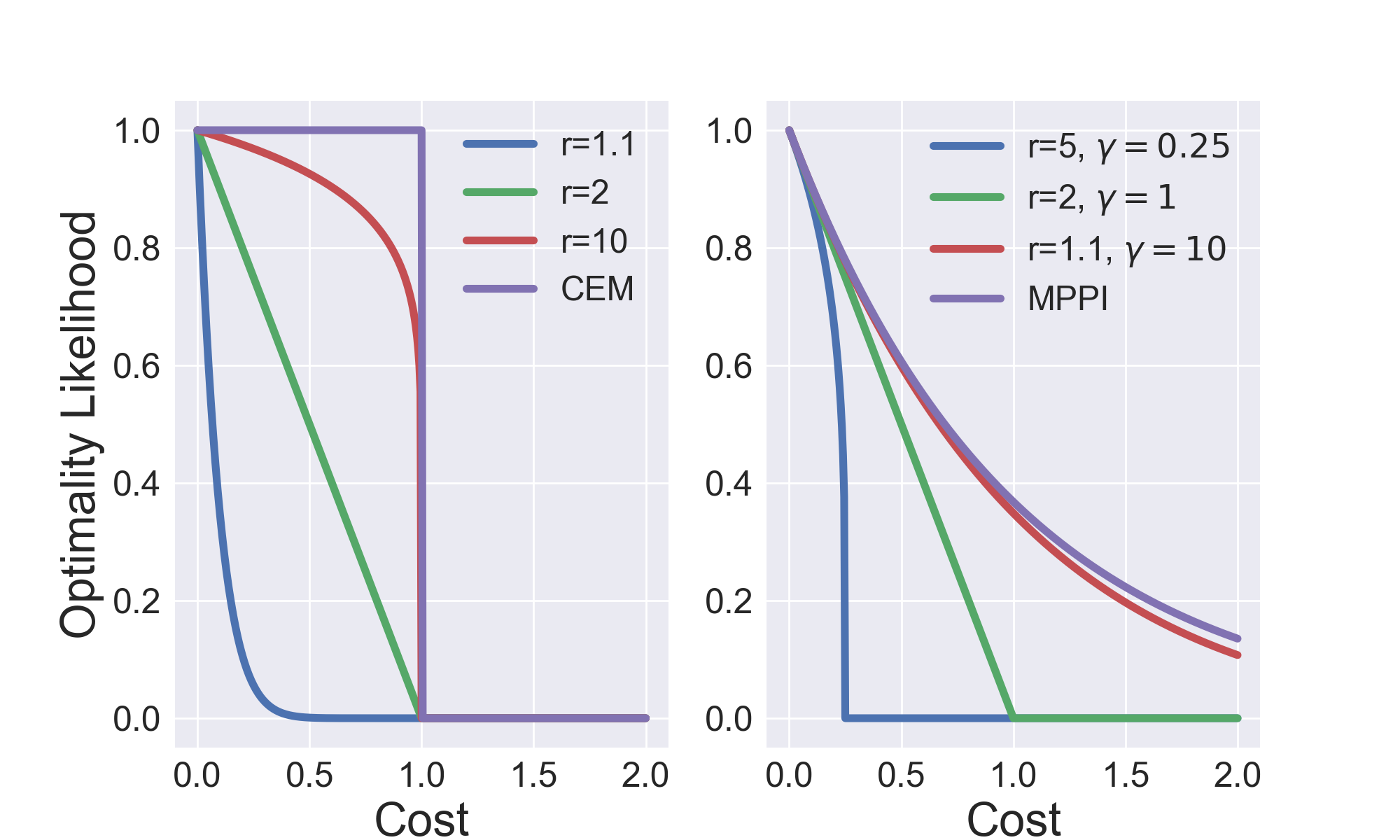
Figure 1: Reparameterized exprsubscript𝑟\exp_{r} (Eq. 28)Eq. 28(\lx@cref{creftype~refnum}{eq:reparameterization}). Left: r𝑟r is varied with fixed γ=1𝛾1\gamma=1. It is clear that exprsubscript𝑟absent\exp_{r}\to CEM as r𝑟r\to\infty. Right: γ𝛾\gamma is adjusted accordingly such that exprsubscript𝑟absent\exp_{r}\to MPPI as r1𝑟1r\to 1.

IV-A Effect of exprsubscript𝑟\exp_{r}

To facilitate the analysis, we focus on the exprsubscript𝑟\exp_{r} term in Eq. 10. Reparametrizing λ~=(r1)γ~𝜆𝑟1𝛾\tilde{\lambda}=(r-1)\gamma, we get

expr(λ~1J)=(1Jγ)+1r1={exp(1r1log(1Jγ)),J<γ0,Jγ,subscript𝑟superscript~𝜆1𝐽superscriptsubscript1𝐽𝛾1𝑟1cases1𝑟11𝐽𝛾𝐽𝛾otherwise0𝐽𝛾otherwise\begin{split}\exp_{r}(-\tilde{\lambda}^{-1}J)&=\left(1-\frac{J}{\gamma}\right)_{+}^{\frac{1}{r-1}}\\ &=\begin{cases}\exp\left(\frac{1}{r-1}\log\left(1-\frac{J}{\gamma}\right)\right),\,J<\gamma\\ 0,\hskip 96.0002ptJ\geq\gamma\end{cases},\end{split} (28)

where γ𝛾\gamma is now the threshold beyond which the optimality weight is set to 0. The reparameterization adjusts the original parameter λ~~𝜆\tilde{\lambda} at every iteration to maintain the same threshold γ𝛾\gamma, which is a more intuitive parameter. In addition, we have observed that the reparameterized framework is easier to tune and achieves better performance than the original formulation. Therefore, we focus our analysis and simulations on only the reparameterized version hereon after. Note that in practice, it is easier to define an elite fraction, which adjusts γ𝛾\gamma based on the scale of the costs, instead of using γ𝛾\gamma for easier tuning.

Figure 1 illustrates the shapes of the function corresponding to different r𝑟r and γ𝛾\gamma values. For J<γ𝐽𝛾J<\gamma, as r𝑟r\rightarrow\infty, expr(λ~1J)1subscript𝑟superscript~𝜆1𝐽1\exp_{r}(-\tilde{\lambda}^{-1}J)\rightarrow 1. Hence, expr(λ~1J)subscript𝑟superscript~𝜆1𝐽\exp_{r}(-\tilde{\lambda}^{-1}J) converges pointwise to the step function 𝟏{Jγ}subscript1𝐽𝛾\bm{1}_{\{J\leq\gamma\}} with r𝑟r\to\infty. On the other hand, for any 0<Jγ<10𝐽𝛾10<\frac{J}{\gamma}<1, we have that

expr(λ~10)expr(λ~1J)=exp(1r1log(1Jγ)),subscript𝑟superscript~𝜆10subscript𝑟superscript~𝜆1𝐽1𝑟11𝐽𝛾\frac{\exp_{r}(-\tilde{\lambda}^{-1}0)}{\exp_{r}(-\tilde{\lambda}^{-1}J)}=\exp\left(-\frac{1}{r-1}\log\left(1-\frac{J}{\gamma}\right)\right), (29)

which tends to 0 as r1𝑟1r\to 1. Hence, exp(1r1log(1Jγ))1𝑟11𝐽𝛾\exp\left(\frac{1}{r-1}\log\left(1-\frac{J}{\gamma}\right)\right) converges to 𝟏{J=0}subscript1𝐽0\bm{1}_{\{J=0\}} as r1𝑟1r\to 1.

IV-B Variance Reduction

With the connection to SS, the effect of Tsallis divergence can be analyzed through the equivalent problem formulation in optimization. In Section III-A, it is shown that Tsallis VI-SOC corresponds to an upper bound of SS-SOC with objective

θ=argmaxθ𝔼π(U;θ)[expr(λ~1J)].superscript𝜃subscriptargmax𝜃subscript𝔼𝜋𝑈𝜃delimited-[]subscript𝑟superscript~𝜆1𝐽\theta^{*}=\operatorname*{arg\,max}_{\theta}\mathbb{E}_{\pi(U;\theta)}\left[\exp_{r}(-\tilde{\lambda}^{-1}J)\right]. (30)

The variance reduction effect can be analyzed through the coefficient of Absolute Risk Aversion (ARA) [33]

A(J)=S′′(J)S(J),𝐴𝐽superscript𝑆′′𝐽superscript𝑆𝐽A(J)=-\frac{S^{\prime\prime}(J)}{S^{\prime}(J)}, (31)

for the optimization problem

minθ𝔼p(X|U),π(U;θ)[S(J(X,U))],subscript𝜃subscript𝔼𝑝conditional𝑋𝑈𝜋𝑈𝜃delimited-[]𝑆𝐽𝑋𝑈\min_{\theta}\mathbb{E}_{p(X|U),\pi(U;\theta)}[S(J(X,U))], (32)

where Tsallis VI-SOC corresponds to S(J)=expr(λ~1J)𝑆𝐽subscript𝑟superscript~𝜆1𝐽S(J)=\exp_{r}(-\tilde{\lambda}^{-1}J)). The ARA coefficient measures a scaled ratio of terms corresponding to the mean and variance terms in the Taylor series expansion of the objective. Negative value of the coefficient corresponds to a risk-averse objective, and positive value of the coefficient corresponds to risk-seeking behavior.111ARA is originally used for utility maximization, where a larger ARA corresponds to greater risk aversion. This is the opposite in our case when we are performing cost minimization.The ARA coefficient of Tsallis VI-SOC is

ATsallis(J)=r2(r1)(γJ).subscript𝐴Tsallis𝐽𝑟2𝑟1𝛾𝐽A_{\text{Tsallis}}(J)=-\frac{r-2}{(r-1)(\gamma-J)}. (33)

The ARA coefficients for MPPI and CEM are

AMPPI(J)subscript𝐴MPPI𝐽\displaystyle A_{\text{MPPI}}(J) =1λ,absent1𝜆\displaystyle=\frac{1}{\lambda}, (34)
ACEM(J)subscript𝐴CEM𝐽\displaystyle A_{\text{CEM}}(J) =limkktanh(12k(γJ)).absentsubscript𝑘𝑘12𝑘𝛾𝐽\displaystyle=\lim_{k\rightarrow\infty}-k\tanh\left(\frac{1}{2}k(\gamma-J)\right). (35)

Since AMPPIsubscript𝐴MPPIA_{\text{MPPI}} is a positive constant, it corresponds to a risk-seeking algorithm. For a cost below the elite threshold, J<γ𝐽𝛾J<\gamma, ACEM=subscript𝐴CEMA_{\text{CEM}}=-\infty and ATsallis0less-than-or-greater-thansubscript𝐴Tsallis0A_{\text{Tsallis}}\lessgtr 0 for r2less-than-or-greater-than𝑟2r\lessgtr 2. This leads to the Tsallis VI-SOC framework achieving lower variance than MPPI. For the same elite threshold γ𝛾\gamma and a properly selected r𝑟r, we hypothesize that Tsallis VI-SOC results in lower mean cost than CEM since CEM penalizes variance infinitely harder than the mean and assigns equal weights to all elite samples. A more detailed analysis and the derivation of ARA coefficient are included in Section SM-3 of the supplementary material.

V Model Predictive Control Algorithm

Algorithm 1 Tsallis Variational Inference MPC
1:  Given: p(x0)𝑝subscript𝑥0p(x_{0}): initial state distribution; N𝑁N: number of policy samples; M𝑀M: number of state samples; T𝑇T: MPC horizon; Tsuperscript𝑇T^{\prime}: number of MPC steps; K𝐾K: optimization iterations per MPC step
2:  Initialize Θ00subscriptsuperscriptΘ00\Theta^{0}_{0}
3:  {x0n,m}n,m=1N,Mp(x0)similar-tosuperscriptsubscriptsuperscriptsubscript𝑥0𝑛𝑚𝑛𝑚1𝑁𝑀𝑝subscript𝑥0\{x_{0}^{n,m}\}_{n,m=1}^{N,M}\sim p(x_{0})
4:  for t=0superscript𝑡0t^{\prime}=0 to T1superscript𝑇1T^{\prime}-1 do
5:     for k=0𝑘0k=0 to K𝐾K do
6:        for n=1𝑛1n=1 to N𝑁N in parallel do
7:           for m=1𝑚1m=1 to M𝑀M in parallel do
8:              Xn,m,Un=frollout(x0n,m,Θtk)superscript𝑋𝑛𝑚superscript𝑈𝑛subscript𝑓rolloutsuperscriptsubscript𝑥0𝑛𝑚subscriptsuperscriptΘ𝑘superscript𝑡X^{n,m},U^{n}=f_{\text{rollout}}(x_{0}^{n,m},\Theta^{k}_{t^{\prime}})
9:              Jn,m=fcost(Xn,m,Un)superscript𝐽𝑛𝑚subscript𝑓costsuperscript𝑋𝑛𝑚superscript𝑈𝑛J^{n,m}=f_{\text{cost}}(X^{n,m},U^{n})
10:           end for
11:           Jn=1Mm=1Mf(Jn,mminJn,mmaxJn,mminJn,m)superscript𝐽𝑛1𝑀superscriptsubscript𝑚1𝑀𝑓superscript𝐽𝑛𝑚superscript𝐽𝑛𝑚superscript𝐽𝑛𝑚superscript𝐽𝑛𝑚J^{n}=\frac{1}{M}\sum_{m=1}^{M}f(\frac{J^{n,m}-\min J^{n,m}}{\max J^{n,m}-\min J^{n,m}})
12:        end for
13:        Θtk+1=fupdate({Jn,Un}n=1N)subscriptsuperscriptΘ𝑘1superscript𝑡subscript𝑓updatesuperscriptsubscriptsuperscript𝐽𝑛superscript𝑈𝑛𝑛1𝑁\Theta^{k+1}_{t^{\prime}}=f_{\text{update}}(\{J^{n},U^{n}\}_{n=1}^{N})
14:     end for
15:     Execute qK(ut,0)superscript𝑞𝐾subscript𝑢superscript𝑡0q^{K}(u_{t^{\prime},0})
16:     Θt+10=frecede(ΘtK)subscriptsuperscriptΘ0superscript𝑡1subscript𝑓recedesubscriptsuperscriptΘ𝐾superscript𝑡\Theta^{0}_{t^{\prime}+1}=f_{\text{recede}}(\Theta^{K}_{t^{\prime}})
17:  end for

With the update laws in Section II-D and a choice of the optimality likelihood function f𝑓f, we propose the novel Tsallis VI-MPC algorithm, summarized in Algorithm 1.

Given the initial state distribution p(x0)𝑝subscript𝑥0p(x_{0}) and a prior policy distribution, N×M𝑁𝑀N\times M initial states are sampled. Given the initial states, N𝑁N control trajectories are sampled from the policy distribution. For each control trajectory sample, M𝑀M state trajectories are propagated for a total of N×M𝑁𝑀N\times M rollouts. The state transitions at each timestep are sampled from the stochastic dynamics F(x,u,ϵ)𝐹𝑥𝑢italic-ϵF(x,u,\epsilon) where ϵitalic-ϵ\epsilon corresponds to system stochasticity (zero mean Gaussian ϵ𝒩(0,σϵ2𝐈)similar-toitalic-ϵ𝒩0subscriptsuperscript𝜎2italic-ϵ𝐈\epsilon\sim\mathcal{N}(0,\sigma^{2}_{\epsilon}\bf{I}) used in this paper). The cost of each trajectory is normalized to [0,1]01[0,1] for numerical stability and easier tuning. Depending on the choice of policy distribution class, the policy parameters are updated based on the update laws in Section II-D.
Refer to caption
Refer to caption
Refer to caption
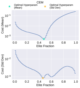
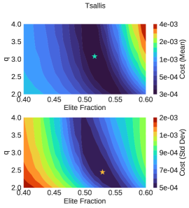
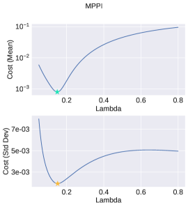
Figure 2: Comparison of mean cost and cost variance for the numerical analysis system Eq. 36. The cost achieved using the updated u𝑢u from a single update step, averaged over 409640964096 different seeds, is shown over the entire range of the hyperparameter set for CEM, MPPI and Tsallis VI-SOC. The hyperparameters which minimize the mean and standard deviation of the cost are shown as a cyan and orange star respectively.
TABLE III: Comparison on a simple single stage stochastic optimization problem Eq. 36. The best values are boldfaced.
Algorithm Cost (Mean) Cost (Std Dev) Mean Control Error
Tsallis 0.000 2650.0002650.000\,265 0.000 4800.0004800.000\,480 0.022 0420.0220420.022\,042
CEM 0.000 5360.0005360.000\,536 0.000 9260.0009260.000\,926 0.050 4150.0504150.050\,415
MPPI 0.000 7950.0007950.000\,795 0.001 1570.0011570.001\,157 0.043 3110.0433110.043\,311
Refer to caption
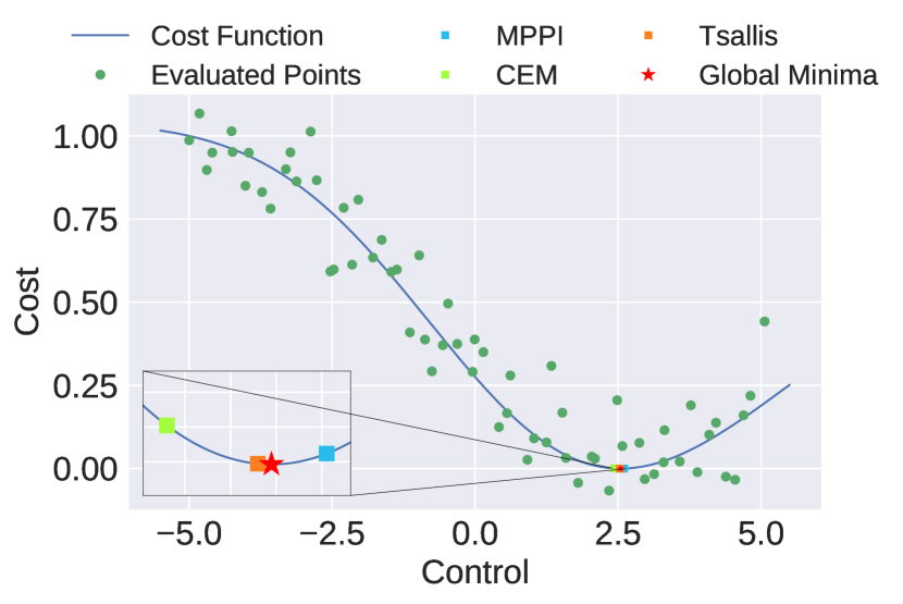
Figure 3: A comparison of the updated means for CEM, MPPI and Tsallis VI-SOC using the best set of hyperparameters on a single realization of 646464 noisy samples of u𝑢u (green) for the numerical analysis system. Each sample is a noisy realization.

For the first iteration, we perform additional warm-up iterations by running the optimization loop (line 5 to 14) for a larger Kwarmupsubscript𝐾warmupK_{\text{warmup}} iterations before executing the first control and performing K𝐾K optimization iterations in the ensuing MPC steps.

Control Selection: With the optimized policy distribution from the VI-SOC framework, the control to be executed on the real system is selected differently based on the choice of policy class. For the unimodal Gaussian policy, the mean of the distribution is used. For the Gaussian mixture policy, the mean of the model with the highest mixture weight is executed. In terms of the Stein policy, the Stein particle with the highest weight is used.

Receding Horizon: After the control execution, the policy distribution is shifted to warm start the optimization at the next MPC timestep. Let θsuperscript𝜃\theta^{\prime} be the next iteration’s starting sequence and θ𝜃\theta be the current iteration’s sequence and set θt=θt+1subscriptsuperscript𝜃𝑡subscript𝜃𝑡1\theta^{\prime}_{t}=\theta_{t+1} for t=0,,T2𝑡0𝑇2t=0,...,T-2. Finally, set the last item in the new sequence as θT1=θT1subscriptsuperscript𝜃𝑇1subscript𝜃𝑇1\theta^{\prime}_{T-1}=\theta_{T-1}. This is known as the receding horizon technique in MPC. Note that in Algorithm 1, Θ={θ0,,θT1}Θsubscript𝜃0subscript𝜃𝑇1\Theta=\{\theta_{0},\cdots,\theta_{T-1}\}.

VI Simulations

In this section, we compare the proposed Tsallis VI-MPC algorithm against MPPI and CEM, which represent state-of-the-art sampling-based SOC algorithms. Since in practice, the shape functions used in SS-SOC corresponds to the ones which result in MPPI and CEM, we have chosen to only compare to MPPI and CEM. We first validate our analysis on a simple numerical experiment. We then showcase the scalability and performance of the Tsallis VI-MPC algorithm on 2D point mass, quadcopter, ant, manipulator and humanoid systems in simulation under the 3 aforementioned policy distributions.

VI-A Numerical Analysis

We verify the analysis in Section IV-B that Tsallis VI-SOC results in greater variance reduction by comparing the exprsubscript𝑟\exp_{r} cost transform with the CEM and MPPI cost transforms on the following simple single-stage stochastic optimization problem:

minu𝔼ξ[λ2eλ2(λσ22u)erf(λσ2u2σ)cd+0.1ξ],subscript𝑢subscript𝔼𝜉delimited-[]𝜆2superscript𝑒𝜆2𝜆superscript𝜎22𝑢erf𝜆superscript𝜎2𝑢2𝜎𝑐𝑑0.1𝜉\min_{u}\,\mathbb{E}_{\xi}\left[\frac{-\frac{\lambda}{2}e^{\frac{\lambda}{2}(\lambda\sigma^{2}-2u)}\operatorname{erf}\left(\frac{\lambda\sigma^{2}-u}{\sqrt{2}\sigma}\right)-c}{d}+0.1\xi\right], (36)

where ξ𝒩(0,1)similar-to𝜉𝒩01\xi\sim\mathcal{N}(0,1), erferf\operatorname{erf} is the corresponding error function, the constants λ𝜆\lambda and σ𝜎\sigma are chosen to be λ=0.2,σ=2.5formulae-sequence𝜆0.2𝜎2.5\lambda=0.2,\sigma=2.5, and c𝑐c and d𝑑d are chosen such that the noiseless objective function is normalized between 00 and 111 for u[5,5]𝑢55u\in[-5,5]. Figure 3 plots the objective function near its minimum and the noisy objective values.

To ensure that only the weight computation of the three methods is tested, we sample 646464 instances of u𝑢u uniformly from [5,5]55[-5,5] and use the same set of samples for all three methods. We use the update law corresponding to the unimodal Gaussian with fixed variance for each algorithm and compare the resulting mean and standard deviation of the cost obtained from each method after a single optimization iteration. A grid search is performed over 409640964096 different hyperparameters, and the optimization metric is computed as the cost averaged over 409640964096 random seeds. The results for the best performing hyperparameters are shown in Table III and agree with our intuition that the objective function of Tsallis VI-SOC should result in a lower variance compared to MPPI and a lower mean compared to CEM. In addition, in Fig. 2, we observe that mean cost increases slower as the elite fraction decreases from the optimal value than when increases, while the opposite is true for cost standard deviation.

VI-B Controls and Robotics Systems

The dynamics for the planar navigation and quadcopter tasks are solved via an Euler discretization. Details of the dynamics can be found in Section SM-4. For the manipulator, ant, and humanoid tasks, we use the GPU-accelerated Isaac-Gym [34] to sample trajectory rollouts in parallel. Additional system stochasticity is injected to each system through the controls channel such that F(xt,ut,ϵt)=F(xt,ut+ϵt)𝐹subscript𝑥𝑡subscript𝑢𝑡subscriptitalic-ϵ𝑡𝐹subscript𝑥𝑡subscript𝑢𝑡subscriptitalic-ϵ𝑡F(x_{t},u_{t},\epsilon_{t})=F(x_{t},u_{t}+\epsilon_{t}).

The hyperparameters and system configurations for all simulations are included in Section SM-4. To ensure fair comparisons, all hyperparameters for each method are tuned using a combination of the TPE algorithm [35] from the Neural Network Intelligence (NNI) AutoML framework and hand tuning.

TABLE IV: Comparisons of mean and standard deviation of cost against MPPI and CEM on different systems and policy classes. The policy classes are defined as Unimodal Gaussian (UG), Gaussian Mixture (GM), and Stein (S). Note that the negative of the reward is used for the locomotion tasks (ant and humanoid). The best mean cost and cost variance for each system-policy distribution pair is boldfaced. The mean and standard deviation reduction percentages are included to the right where positive values correspond to a reduction.
MPPI CEM Tsallis Tsallis vs MPPI Tsallis vs CEM
System Policy Mean Std Mean Std Mean Std ΔΔ\DeltaMean% ΔΔ\DeltaStd% ΔΔ\DeltaMean% ΔΔ\DeltaStd%
Planar Navigation
UG
30 023.7330023.7330\,023.73 3644.073644.073644.07 34 617.4734617.4734\,617.47 2523.342523.342523.34 28 714.7428714.7428\,714.74 570.23570.23570.23 4.364.364.36 84.3584.3584.35 17.0517.0517.05 77.4077.4077.40
GM
39 313.8439313.8439\,313.84 8924.768924.768924.76 53 385.3053385.3053\,385.30 5493.975493.975493.97 31 369.2231369.2231\,369.22 5683.235683.235683.23 20.2120.2120.21 36.3236.3236.32 41.2441.2441.24 3.44-3.44-3.44
S 38 224.9538224.9538\,224.95 5169.925169.925169.92 38 847.5638847.5638\,847.56 6641.786641.786641.78 33 324.4833324.4833\,324.48 4006.434006.434006.43 12.8212.8212.82 22.5022.5022.50 14.2214.2214.22 39.6839.6839.68
Quadcopter
UG
15 266.1515266.1515\,266.15 1374.041374.041374.04 15 756.7515756.7515\,756.75 2707.082707.082707.08 14 673.4014673.4014\,673.40 1458.361458.361458.36 3.883.883.88 6.14-6.14-6.14 6.886.886.88 46.1346.1346.13
GM
22 145.5122145.5122\,145.51 4007.334007.334007.33 17 654.0817654.0817\,654.08 1593.861593.861593.86 16 430.5616430.5616\,430.56 1498.241498.241498.24 25.8125.8125.81 62.6162.6162.61 6.936.936.93 6.06.06.0
S 29 238.2529238.2529\,238.25 5084.315084.315084.31 21 064.7321064.7321\,064.73 2218.022218.022218.02 15 976.0215976.0215\,976.02 1218.321218.321218.32 45.3645.3645.36 76.0476.0476.04 24.1624.1624.16 45.0745.0745.07
Franka
UG
64.1764.1764.17 8.438.438.43 66.3766.3766.37 18.4018.4018.40 57.4157.4157.41 5.535.535.53 10.610.610.6 34.534.534.5 13.613.613.6 70.170.170.1
GM
67.1667.1667.16 8.268.268.26 68.7468.7468.74 13.0113.0113.01 59.1559.1559.15 5.375.375.37 11.9811.9811.98 34.934.934.9 13.9013.9013.90 58.558.558.5
S 72.4072.4072.40 4.224.224.22 80.3580.3580.35 13.9613.9613.96 71.7771.7771.77 3.293.293.29 0.80.80.8 21.421.421.4 10.710.710.7 76.476.476.4
Ant
UG
528.7-528.7-528.7 54.154.154.1 652.6-652.6-652.6 26.726.726.7 692.9-692.9-692.9 37.237.237.2 31.131.131.1 31.331.331.3 6.26.26.2 39.0-39.0-39.0
GM
621.0-621.0-621.0 55.555.555.5 659.1-659.1-659.1 53.653.653.6 663.8-663.8-663.8 36.336.336.3 6.96.96.9 34.734.734.7 0.70.70.7 32.432.432.4
S 673.7-673.7-673.7 36.136.136.1 670.0-670.0-670.0 32.232.232.2 677.4-677.4-677.4 13.413.413.4 0.60.60.6 62.862.862.8 1.11.11.1 58.358.358.3
Humanoid
UG
423.79-423.79-423.79 233.81233.81233.81 660.80-660.80-660.80 208.48208.48208.48 899.27-899.27-899.27 80.0980.0980.09 112.20112.20112.20 65.7465.7465.74 36.0936.0936.09 61.5861.5861.58
GM
592.85-592.85-592.85 170.15170.15170.15 725.92-725.92-725.92 164.92164.92164.92 738.08-738.08-738.08 103.76103.76103.76 24.5024.5024.50 39.0239.0239.02 1.671.671.67 37.0937.0937.09
S 794.69-794.69-794.69 173.96173.96173.96 840.81-840.81-840.81 168.12168.12168.12 919.67-919.67-919.67 105.85105.85105.85 15.7315.7315.73 39.1539.1539.15 9.389.389.38 37.0437.0437.04

VI-B1 Planar Navigation

We first test the different algorithms on a point-mass planar navigation problem. The task is for the point-mass with double-integrator stochastic dynamics to navigate through an obstacle field to reach the target location. The dynamics and obstacle field are set up the same way as [6]. If a crash occurs, a crash cost is incurred and no further movement is allowed.

VI-B2 Quadcopter

We also set up a quadcopter 3-D navigation task. The task is for the quadcopter to reach a target location while avoiding obstacles. The quadcopter dynamics are taken from [36]. The quadcopter task is similiar to the planar navigation task, where the system is expected to fly through a randomly generated forest to reach the target location. If a crash occurs, a crash cost is incurred and no further movement is allowed.

VI-B3 Franka Manipulator

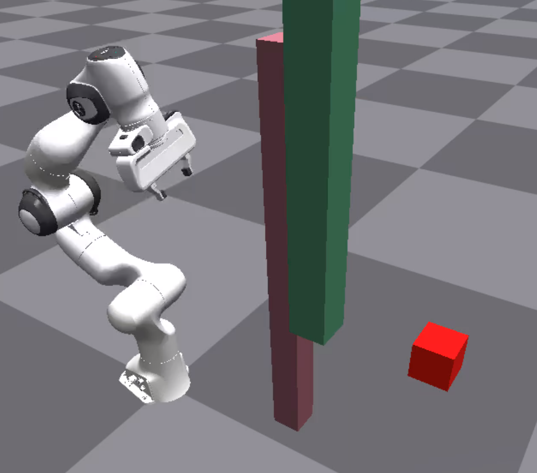
We next test on the Franka manipulator modified to have 7-DOF by removing the last joint and fixing the fingers. The objective of this task is to move the end effector around the obstacles to the goal. An illustration of the task is in Fig. 4. It is worth noting that no crash cost is in place for the Franka manipulator. Instead, contact is included as a part of the simulation dynamics.
Refer to caption
Figure 4: Task setup for Franka manipulator. The goal is to reach the red block while avoiding the pink and green obstacles.

VI-B4 Ant

We also consider the task of locomotion. We test on the ant system, which has 292929 state dimensions, 888 control dimensions, and is a widely used testbed for RL algorithms.

VI-B5 Humanoid

Finally, we test our approach on the complex humanoid locomotion task. The humanoid system has 565656 state dimensions, 212121 control dimensions, and has very unstable dynamics.

VI-C Discussion

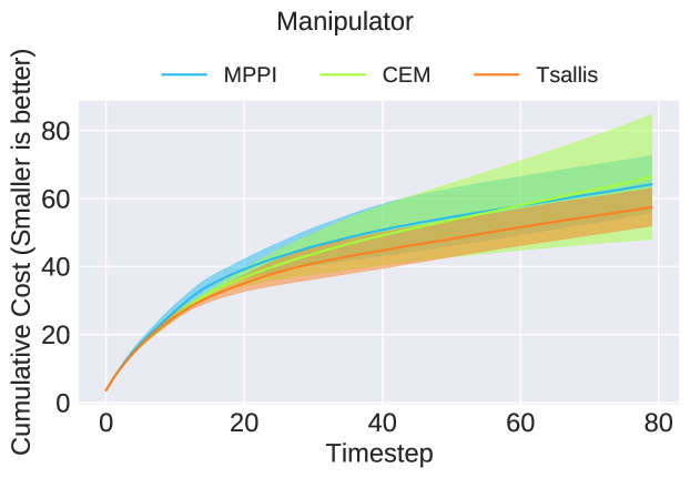
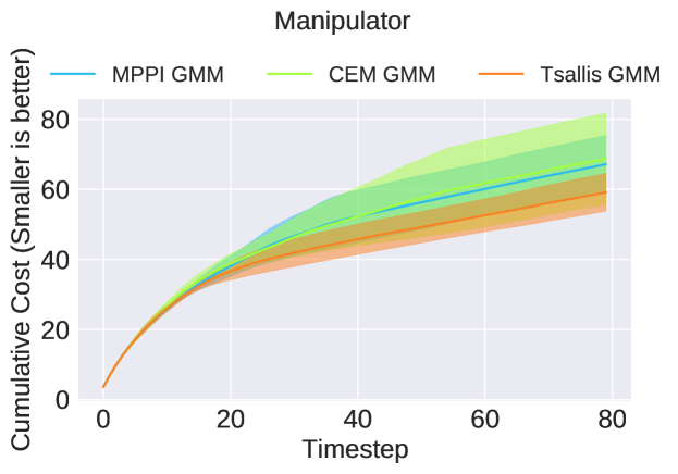
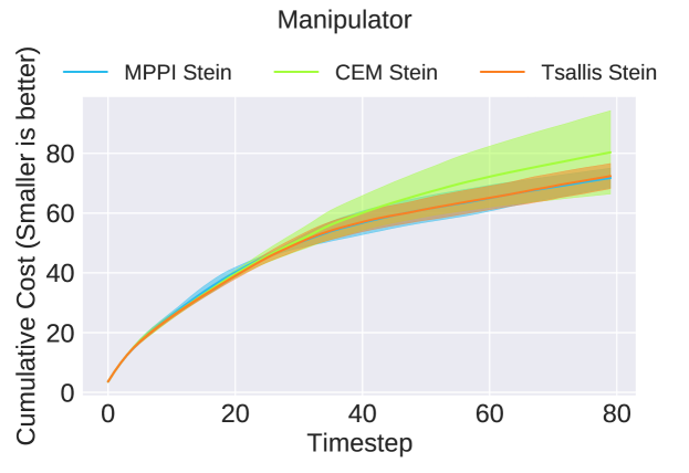
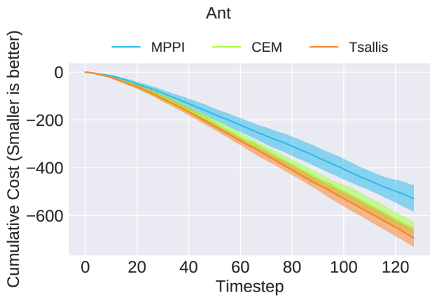
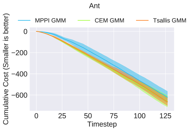
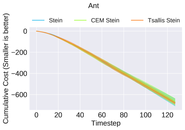
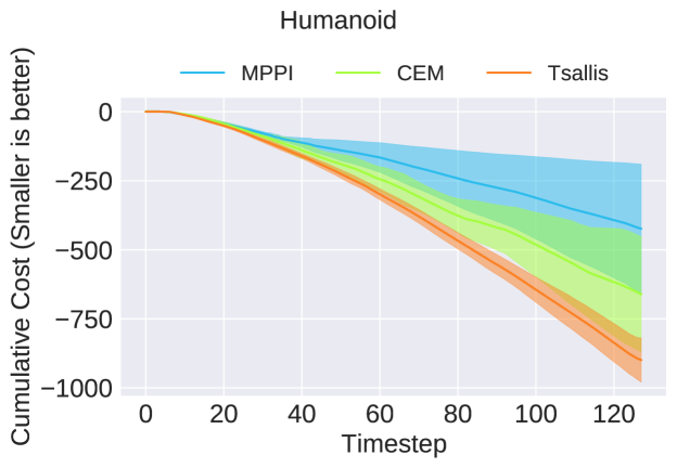
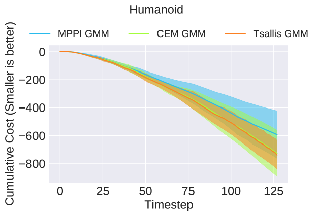
In Table IV, we can see the results of each experiment summarized between each robotic system, policy parameterization, and choice of SOC framework. Across all systems we can see Tsallis VI-MPC results in lower means and variances in most policy parameterizations. The trend continues even as the complexity of the dynamics increases showing that the flexibility provided by the VI-MPC framework is useful even in high dimensional systems.

First in the planar navigation case, we see that Tsallis VI-MPC outperforms the other algorithms in almost all policy parameterizations. During testing, there was high variability in the trajectories computed by each algorithm. The best performing algorithms would have a large increase in velocity towards the goal state, and would have enough variation in sampled trajectories to ”see“ obstacles via large costs in order to avoid them. When comparing the trajectories computed through the GM policy parameterization we tend to see a reduced ability to stabilize at the goal resulting in larger costs overall when compared to other parameterizations. For these systems, the Stein policy results in longer trajectories to the goal. Next in the Quadcopter experiments, we observe that the Tsallis VI-MPC outperforms both MPPI and CEM in mean cost for the unimodal Gaussian and Stein policies. When looking at the high dimensional simulation environments, we see the same trend of Tsallis VI-MPC reducing the mean and variance in comparison to CEM and MPPI holds even for complex systems with contact dynamics.

The performance of the Tsallis VI-MPC can be attributed to the ability of the algorithm to sample policies that are low cost (via the elite fraction), but then improve beyond the CEM by performing the cost weighted averaging similar to MPPI. These characteristics of Tsallis VI-MPC are additionally heavily related to the choice of hyperparameters. From hand tuning, we observe that reducing the elite fraction generally results in lower mean cost but higher standard deviation and vice versa. As the cost transform approaches that of CEM or MPPI, the mean and standard deviation approaches their corresponding value. This verifies that the Tsallis VI-SOC framework can be thought of as an interpolation between CEM and MPPI to a certain degree. The best performing configuration is usually somewhere in between these two extremes.

Finally note that even though the Tsallis VI-SOC framework is typically used over multiple iterations in optimization schemes where the parameters can evolve as the optimization progresses, we have shown the benefits even in MPC mode, where a single iteration of optimization is performed, reiterating the empirical result that a single step has higher reduction in mean cost and variance compared to traditional MPC methods.

VII Conclusion

We present a generalized Variational Inference-Stochastic Optimal Control framework using Tsallis divergence, which allows for additional control of the cost/reward transform and results in lower cost/reward variance. We provide a unifying study of the connections between Tsallis VI-SOC, MPPI, CEM, and SS methods. The performance and variance reduction benefits of the proposed Tsallis VI-SOC framework is verified analytically and numerically. We further showcase advantages of the Tsallis VI-MPC algorithm against MPPI and CEM on 5 different systems with 3 different policy distributions. We leave 2 extensions of this work as future research directions: 1. Implementation of the proposed algorithm on real systems; 2. Comparison against VI-MPC algorithms using other generalized divergences.

Acknowledgments

This work is supported by NASA Langley and the NSF-CPS award #1932288. This work is supported by Sandia National Laboratories, a multimission laboratory managed and operated by National Technology and Engineering Solutions of Sandia, LLC., a wholly owned subsidiary of Honeywell International, Inc., for the U.S. Department of Energy’s National Nuclear Security Administration under contract DE-NA-0003525. Additionally, this work is supported by NASA LaRC.

References

SM-1 Derivation of Optimal Distribution

To solve for the optimal distribution, we first formulate the Lagrangian as

(U,λ,α)𝑈𝜆𝛼\displaystyle\mathcal{L}(U,\lambda,\alpha) =λ1𝔼q(U)[J]+𝒟r(q(U)p(U))absentsuperscript𝜆1subscript𝔼𝑞𝑈delimited-[]𝐽subscript𝒟𝑟conditional𝑞𝑈𝑝𝑈\displaystyle=\lambda^{-1}\mathbb{E}_{q(U)}[J]+\mathcal{D}_{r}\left({q(U)}\parallel{p(U)}\right) (37)
+α(1q(U)dU),𝛼1𝑞𝑈d𝑈\displaystyle+\alpha\left(1-\int q(U){\textnormal{d}}U\right), (38)

which can be solved by setting q=0𝑞0\frac{\partial\mathcal{L}}{\partial q}=0 as

q𝑞\displaystyle\frac{\partial\mathcal{L}}{\partial q} =λ1J+rr1(q(U)p(U))r1α=0absentsuperscript𝜆1𝐽𝑟𝑟1superscript𝑞𝑈𝑝𝑈𝑟1𝛼0\displaystyle=\lambda^{-1}J+\frac{r}{r-1}\left(\frac{q(U)}{p(U)}\right)^{r-1}-\alpha=0 (39)
q(U)absentsuperscript𝑞𝑈\displaystyle\Rightarrow q^{*}(U) =(r1r)1r1(αλ1J)1r1p(U).absentsuperscript𝑟1𝑟1𝑟1superscript𝛼superscript𝜆1𝐽1𝑟1𝑝𝑈\displaystyle=\left(\frac{r-1}{r}\right)^{\frac{1}{r-1}}\left(\alpha-\lambda^{-1}J\right)^{\frac{1}{r-1}}p(U). (40)

Setting λ1=α(r1)λ~1superscript𝜆1𝛼𝑟1superscript~𝜆1\lambda^{-1}=\alpha(r-1)\tilde{\lambda}^{-1}, we get

q(U)superscript𝑞𝑈\displaystyle q^{*}(U) =(α(r1)r)1r1(1(r1)λ~1J)1r1p(U)absentsuperscript𝛼𝑟1𝑟1𝑟1superscript1𝑟1superscript~𝜆1𝐽1𝑟1𝑝𝑈\displaystyle=\left(\frac{\alpha(r-1)}{r}\right)^{\frac{1}{r-1}}\left(1-(r-1)\tilde{\lambda}^{-1}J\right)^{\frac{1}{r-1}}p(U) (41)
=(α(r1)r)1r1expr(λ~1J)p(U).absentsuperscript𝛼𝑟1𝑟1𝑟1subscript𝑟superscript~𝜆1𝐽𝑝𝑈\displaystyle=\left(\frac{\alpha(r-1)}{r}\right)^{\frac{1}{r-1}}\exp_{r}\left(-\tilde{\lambda}^{-1}J\right)p(U). (42)

We now use the constraint that q(U)dU=1𝑞𝑈d𝑈1\int q(U)\,{\textnormal{d}}U=1 by integrating both sides to get

1=(α(r1)r)1r1expr(λ~1J)p(U)dU1superscript𝛼𝑟1𝑟1𝑟1subscript𝑟superscript~𝜆1𝐽𝑝𝑈d𝑈\displaystyle 1=\left(\frac{\alpha(r-1)}{r}\right)^{\frac{1}{r-1}}\int\exp_{r}\left(-\tilde{\lambda}^{-1}J\right)p(U)\,{\textnormal{d}}U (43)
\displaystyle\Rightarrow (α(r1)r)1r1=1expr(λ~1J)p(U)dU.superscript𝛼𝑟1𝑟1𝑟11subscript𝑟superscript~𝜆1𝐽𝑝𝑈d𝑈\displaystyle\left(\frac{\alpha(r-1)}{r}\right)^{\frac{1}{r-1}}=\frac{1}{\int\exp_{r}\left(-\tilde{\lambda}^{-1}J\right)p(U)\,{\textnormal{d}}U}. (44)

Plugging the normalizing constants back in we can get the optimal policy qsuperscript𝑞q^{*} to be

q(U)=expr(λ~1J)p(U)expr(λ~1J)p(U)dU.superscript𝑞𝑈subscript𝑟superscript~𝜆1𝐽𝑝𝑈subscript𝑟superscript~𝜆1𝐽𝑝𝑈d𝑈q^{*}(U)=\frac{\exp_{r}\left(-\tilde{\lambda}^{-1}J\right)p(U)}{\int\exp_{r}\left(-\tilde{\lambda}^{-1}J\right)p(U)\,{\textnormal{d}}U}. (45)

SM-2 Derivation of Update Laws

For each of the following update laws, we make use of the following equality:

πk+1(U)superscript𝜋𝑘1𝑈\displaystyle\pi^{k+1}(U) =argminπ(U)Π𝒟KL(q~(U)π(U))absentsubscriptargmin𝜋𝑈Πsubscript𝒟𝐾𝐿conditionalsuperscript~𝑞𝑈𝜋𝑈\displaystyle=\operatorname*{arg\,min}_{\pi(U)\in\Pi}\mathcal{D}_{KL}\left({\tilde{q}^{*}(U)}\parallel{\pi(U)}\right) (46)
=argminπ(U)Πq~(U)logq~(U)dUq~(U)logπ(U)dU.absentsubscriptargmin𝜋𝑈Πsuperscript~𝑞𝑈superscript~𝑞𝑈d𝑈superscript~𝑞𝑈𝜋𝑈d𝑈\displaystyle=\operatorname*{arg\,min}_{\pi(U)\in\Pi}\int\tilde{q}^{*}(U)\log\tilde{q}^{*}(U){\textnormal{d}}U-\int\tilde{q}^{*}(U)\log\pi(U){\textnormal{d}}U. (47)

We can drop the first term as it doesn’t relate to the argminπ(U)Πsubscriptargmin𝜋𝑈Π\operatorname*{arg\,min}_{\pi(U)\in\Pi}:

=argminπ(U)Πq~(U)logπ(U)dUabsentsubscriptargmin𝜋𝑈Πsuperscript~𝑞𝑈𝜋𝑈d𝑈\displaystyle=\operatorname*{arg\,min}_{\pi(U)\in\Pi}-\int\tilde{q}^{*}(U)\log\pi(U){\textnormal{d}}U (48)
=argmaxπ(U)Πq~(U)logπ(U)dUabsentsubscriptargmax𝜋𝑈Πsuperscript~𝑞𝑈𝜋𝑈d𝑈\displaystyle=\operatorname*{arg\,max}_{\pi(U)\in\Pi}\int\tilde{q}^{*}(U)\log\pi(U){\textnormal{d}}U (49)
=argmaxπ(U)Πn=1Nw(n)logπ(U(n)).absentsubscriptargmax𝜋𝑈Πsuperscriptsubscript𝑛1𝑁superscript𝑤𝑛𝜋superscript𝑈𝑛\displaystyle=\operatorname*{arg\,max}_{\pi(U)\in\Pi}\sum_{n=1}^{N}w^{(n)}\log\pi(U^{(n)}). (50)

SM-2-A Unimodal Gaussian

For the case of a policy class of unimodal Gaussian distributions where the controls utnusubscript𝑢𝑡superscriptsubscript𝑛𝑢u_{t}\in\mathbb{R}^{n_{u}} of each timestep are independent, the p.d.f. for each timestep’s control has the form

𝒩(ut;μt,Σt)=1(2π)nu|Σt|exp(12(utμt)TΣt1(utμt)).𝒩subscript𝑢𝑡subscript𝜇𝑡subscriptΣ𝑡1superscript2𝜋subscript𝑛𝑢subscriptΣ𝑡12superscriptsubscript𝑢𝑡subscript𝜇𝑡TsuperscriptsubscriptΣ𝑡1subscript𝑢𝑡subscript𝜇𝑡\mathcal{N}(u_{t};\mu_{t},\Sigma_{t})=\frac{1}{\sqrt{(2\pi)^{n_{u}}\lvert\Sigma_{t}\rvert}}\exp\left(-\frac{1}{2}(u_{t}-\mu_{t})^{\mathrm{T}}\Sigma_{t}^{-1}(u_{t}-\mu_{t})\right). (51)

where we have that

μtlog𝒩(ut;μt,Σt)subscriptsubscript𝜇𝑡𝒩subscript𝑢𝑡subscript𝜇𝑡subscriptΣ𝑡\displaystyle\nabla_{\mu_{t}}\log\mathcal{N}(u_{t};\mu_{t},\Sigma_{t}) =(utμt)TΣt1absentsuperscriptsubscript𝑢𝑡subscript𝜇𝑡TsuperscriptsubscriptΣ𝑡1\displaystyle=(u_{t}-\mu_{t})^{\mathrm{T}}\Sigma_{t}^{-1} (52)
Σt1log𝒩(ut;μt,Σt)subscriptsuperscriptsubscriptΣ𝑡1𝒩subscript𝑢𝑡subscript𝜇𝑡subscriptΣ𝑡\displaystyle\nabla_{\Sigma_{t}^{-1}}\log\mathcal{N}(u_{t};\mu_{t},\Sigma_{t}) =12Σt12(utμt)(utμt)T.absent12subscriptΣ𝑡12subscript𝑢𝑡subscript𝜇𝑡superscriptsubscript𝑢𝑡subscript𝜇𝑡T\displaystyle=\frac{1}{2}\Sigma_{t}-\frac{1}{2}(u_{t}-\mu_{t})(u_{t}-\mu_{t})^{\mathrm{T}}. (53)

Minimizing the KL divergence between π(U)𝜋𝑈\pi(U) and q~(U)superscript~𝑞𝑈\tilde{q}^{*}(U) and using Eq. 46, we have

πk+1(U)superscript𝜋𝑘1𝑈\displaystyle\pi^{k+1}(U) =argminπ(U)Π𝒟KL(q~(U)π(U))absentsubscriptargmin𝜋𝑈Πsubscript𝒟𝐾𝐿conditionalsuperscript~𝑞𝑈𝜋𝑈\displaystyle=\operatorname*{arg\,min}_{\pi(U)\in\Pi}\mathcal{D}_{KL}\left({\tilde{q}^{*}(U)}\parallel{\pi(U)}\right) (54)
=argmaxμ,Σn=1Nt=0T1w(n)log𝒩(U(n);μt,Σt).absentsubscriptargmax𝜇Σsuperscriptsubscript𝑛1𝑁superscriptsubscript𝑡0𝑇1superscript𝑤𝑛𝒩superscript𝑈𝑛subscript𝜇𝑡subscriptΣ𝑡\displaystyle=\operatorname*{arg\,max}_{\mu,\Sigma}\sum_{n=1}^{N}\sum_{t=0}^{T-1}w^{(n)}\log\mathcal{N}(U^{(n)};\mu_{t},\Sigma_{t}). (55)

Hence, we have that

00\displaystyle 0 =n=1Nw(n)μtlog𝒩(U(n);μt,Σt)absentsuperscriptsubscript𝑛1𝑁superscript𝑤𝑛subscriptsubscript𝜇𝑡𝒩superscript𝑈𝑛subscript𝜇𝑡subscriptΣ𝑡\displaystyle=\sum_{n=1}^{N}w^{(n)}\nabla_{\mu_{t}}\log\mathcal{N}(U^{(n)};\mu_{t},\Sigma_{t}) (56)
00\displaystyle 0 =n=1Nw(n)Σtlog𝒩(ut(n);μt,Σt).absentsuperscriptsubscript𝑛1𝑁superscript𝑤𝑛subscriptsubscriptΣ𝑡𝒩superscriptsubscript𝑢𝑡𝑛subscript𝜇𝑡subscriptΣ𝑡\displaystyle=\sum_{n=1}^{N}w^{(n)}\nabla_{\Sigma_{t}}\log\mathcal{N}(u_{t}^{(n)};\mu_{t},\Sigma_{t}). (57)

Using Eqs. 52 and 53 then results in the update laws

μtsubscript𝜇𝑡\displaystyle\mu_{t} =n=1Nw(n)ut(n)absentsuperscriptsubscript𝑛1𝑁superscript𝑤𝑛superscriptsubscript𝑢𝑡𝑛\displaystyle=\sum_{n=1}^{N}w^{(n)}u_{t}^{(n)} (58)
ΣtsubscriptΣ𝑡\displaystyle\Sigma_{t} =n=1Nw(n)(ut(n)μt)(ut(n)μt)T.absentsuperscriptsubscript𝑛1𝑁superscript𝑤𝑛superscriptsubscript𝑢𝑡𝑛subscript𝜇𝑡superscriptsuperscriptsubscript𝑢𝑡𝑛subscript𝜇𝑡T\displaystyle=\sum_{n=1}^{N}w^{(n)}(u_{t}^{(n)}-\mu_{t})(u_{t}^{(n)}-\mu_{t})^{\mathrm{T}}. (59)

SM-2-B Mixture of Gaussian

For a Gaussian mixture model π(U;θ)𝜋𝑈𝜃\pi(U;\theta) with L𝐿L components with parameters θ{θl}l=1L𝜃superscriptsubscriptsubscript𝜃𝑙𝑙1𝐿\theta\coloneqq\{\theta_{l}\}_{l=1}^{L} and θl{(ϕl,{μl,t,Σl,t}t=0T1)\theta_{l}\coloneqq\{(\phi_{l},\{\mu_{l,t},\Sigma_{l,t}\}_{t=0}^{T-1}) such that

π(U;θ)𝜋𝑈𝜃\displaystyle\pi(U;\theta) =t=0T1πt(ut;θ)absentsuperscriptsubscriptproduct𝑡0𝑇1subscript𝜋𝑡subscript𝑢𝑡𝜃\displaystyle=\prod_{t=0}^{T-1}\pi_{t}(u_{t};\theta) (60)
πt(ut;θ)subscript𝜋𝑡subscript𝑢𝑡𝜃\displaystyle\pi_{t}(u_{t};\theta) l=1Lπm𝒩(ut;μl,Σl).absentsuperscriptsubscript𝑙1𝐿subscript𝜋𝑚𝒩subscript𝑢𝑡subscript𝜇𝑙subscriptΣ𝑙\displaystyle\coloneqq\sum_{l=1}^{L}\pi_{m}\mathcal{N}(u_{t};\mu_{l},\Sigma_{l}). (61)

Directly trying to minimize the KL divergence between π(U;θ)𝜋𝑈𝜃\pi(U;\theta) and q~(U)superscript~𝑞𝑈\tilde{q}^{*}(U) and using Eq. 46 gives us

θsuperscript𝜃\displaystyle\theta^{*} =argmaxθn=1Nt=0T1(w(n)logl=1Lϕl𝒩(ut(n);μl,t,Σl,t)).absentsubscriptargmax𝜃superscriptsubscript𝑛1𝑁superscriptsubscript𝑡0𝑇1superscript𝑤𝑛superscriptsubscript𝑙1𝐿subscriptitalic-ϕ𝑙𝒩superscriptsubscript𝑢𝑡𝑛subscript𝜇𝑙𝑡subscriptΣ𝑙𝑡\displaystyle=\operatorname*{arg\,max}_{\theta}\sum_{n=1}^{N}\sum_{t=0}^{T-1}\left(w^{(n)}\log\sum_{l=1}^{L}\phi_{l}\mathcal{N}(u_{t}^{(n)};\mu_{l,t},\Sigma_{l,t})\right). (62)

However, it is not straightforward to solve Eq. 62 directly.

Instead, we can use the expectation maximization algorithm and introduce the latent variables {Zn}n=1Nsuperscriptsubscriptsubscript𝑍𝑛𝑛1𝑁\{Z_{n}\}_{n=1}^{N}, Zn[L]subscript𝑍𝑛delimited-[]𝐿Z_{n}\in[L] which form a categorical distribution q(Z)𝑞𝑍q(Z) over each of the L𝐿L mixtures and denotes which mixture each sample U(n)superscript𝑈𝑛U^{(n)} was sampled from. Then, we can write logπ(U;θ)𝜋𝑈𝜃\log\pi(U;\theta) as

logπ(U;θ)𝜋𝑈𝜃\displaystyle\log\pi(U;\theta) =q(z)logπ(U;θ)dzabsent𝑞𝑧𝜋𝑈𝜃d𝑧\displaystyle=\int q(z)\log\pi(U;\theta){\textnormal{d}}z (63)
=q(z)logπ(U;θ)p(z|U;θ)p(z|U;θ)dzabsent𝑞𝑧𝜋𝑈𝜃𝑝conditional𝑧𝑈𝜃𝑝conditional𝑧𝑈𝜃d𝑧\displaystyle=\int q(z)\log\frac{\pi(U;\theta)p(z|U;\theta)}{p(z|U;\theta)}{\textnormal{d}}z (64)
=q(z)logp(U,z;θ)p(z|U;θ)dzabsent𝑞𝑧𝑝𝑈𝑧𝜃𝑝conditional𝑧𝑈𝜃d𝑧\displaystyle=\int q(z)\log\frac{p(U,z;\theta)}{p(z|U;\theta)}{\textnormal{d}}z (65)
=q(z)logp(U,z;θ)q(z)dzq(z)logp(z|U;θ)q(z)dzabsent𝑞𝑧𝑝𝑈𝑧𝜃𝑞𝑧d𝑧𝑞𝑧𝑝conditional𝑧𝑈𝜃𝑞𝑧d𝑧\displaystyle=\int q(z)\log\frac{p(U,z;\theta)}{q(z)}{\textnormal{d}}z-\int q(z)\log\frac{p(z|U;\theta)}{q(z)}{\textnormal{d}}z (66)
=F(q,θ)+𝒟KL(qp).absent𝐹𝑞𝜃subscript𝒟𝐾𝐿conditional𝑞𝑝\displaystyle=F(q,\theta)+\mathcal{D}_{KL}\left({q}\parallel{p}\right). (67)

where F(q,θ)𝐹𝑞𝜃F(q,\theta) is the ELBO, and provides a lower bound for the log likelihood logp(U;θ)𝑝𝑈𝜃\log p(U;\theta). Now, to optimize F(q,θ)𝐹𝑞𝜃F(q,\theta), we estimate q(z)𝑞𝑧q(z) via p(z|U;θk)𝑝conditional𝑧𝑈superscript𝜃𝑘p(z|U;\theta^{k}), where θksuperscript𝜃𝑘\theta^{k} is the previous iteration’s parameters. Then, the ELBO becomes

F(q,θ)𝐹𝑞𝜃\displaystyle F(q,\theta) =q(z)logp(U,z;θ)q(z)dzabsent𝑞𝑧𝑝𝑈𝑧𝜃𝑞𝑧d𝑧\displaystyle=\int q(z)\log\frac{p(U,z;\theta)}{q(z)}{\textnormal{d}}z (68)
=q(z)logp(U,z;θ)dzq(z)logq(z)dzabsent𝑞𝑧𝑝𝑈𝑧𝜃d𝑧𝑞𝑧𝑞𝑧d𝑧\displaystyle=\int q(z)\log p(U,z;\theta){\textnormal{d}}z-\int q(z)\log q(z){\textnormal{d}}z (69)
=p(z|U;θk)logp(U,z;θ)dzp(z|U;θk)logp(z|U;θk)dzabsent𝑝conditional𝑧𝑈superscript𝜃𝑘𝑝𝑈𝑧𝜃d𝑧𝑝conditional𝑧𝑈superscript𝜃𝑘𝑝conditional𝑧𝑈superscript𝜃𝑘d𝑧\displaystyle=\int p(z|U;\theta^{k})\log p(U,z;\theta){\textnormal{d}}z-\int p(z|U;\theta^{k})\log p(z|U;\theta^{k}){\textnormal{d}}z (70)
=Q(θ,θk)+H(z|U).absent𝑄𝜃superscript𝜃𝑘𝐻conditional𝑧𝑈\displaystyle=Q(\theta,\theta^{k})+H(z|U). (71)

Since the second term is a function of θksuperscript𝜃𝑘\theta^{k} and thus is not dependent on θ𝜃\theta, it suffices to optimize Q(θ,θk)𝑄𝜃superscript𝜃𝑘Q(\theta,\theta^{k}). To do so, the EM algorithm separates this into two steps:

  1. 1.

    E-step: Compute p(z|U;θk)𝑝conditional𝑧𝑈superscript𝜃𝑘p(z|U;\theta^{k}).

  2. 2.

    M-step: Compute argmaxθQ(θ,θk)subscriptargmax𝜃𝑄𝜃superscript𝜃𝑘\operatorname*{arg\,max}_{\theta}Q(\theta,\theta^{k}).

In our case, we have that

Q(θ,θk)𝑄𝜃superscript𝜃𝑘\displaystyle Q(\theta,\theta^{k}) =p(z|U;θk)logp(U,z;θ)dzabsent𝑝conditional𝑧𝑈superscript𝜃𝑘𝑝𝑈𝑧𝜃d𝑧\displaystyle=\int p(z|U;\theta^{k})\log p(U,z;\theta){\textnormal{d}}z (72)
=𝔼zp(z|U;θk)[n=1Nl=1Lt=0T1𝟙{Zn=l}w(n)(logϕl+log𝒩(ut(n)|μl,t,Σl,t))]absentsubscript𝔼similar-to𝑧𝑝conditional𝑧𝑈superscript𝜃𝑘delimited-[]superscriptsubscript𝑛1𝑁superscriptsubscript𝑙1𝐿superscriptsubscript𝑡0𝑇11subscript𝑍𝑛𝑙superscript𝑤𝑛subscriptitalic-ϕ𝑙𝒩conditionalsuperscriptsubscript𝑢𝑡𝑛subscript𝜇𝑙𝑡subscriptΣ𝑙𝑡\displaystyle=\mathbb{E}_{{z\sim p(z|U;\theta^{k})}}{\left[\sum_{n=1}^{N}\sum_{l=1}^{L}\sum_{t=0}^{T-1}\mathbbm{1}\{Z_{n}=l\}w^{(n)}\left(\log\phi_{l}+\log\mathcal{N}(u_{t}^{(n)}|\mu_{l,t},\Sigma_{l,t})\right)\right]} (73)
=n=1Nl=1Lt=0T1p(Zn=l|ut(n);θk)w(n)(logϕl+log𝒩(ut(n)|μl,t,Σl,t))absentsuperscriptsubscript𝑛1𝑁superscriptsubscript𝑙1𝐿superscriptsubscript𝑡0𝑇1𝑝subscript𝑍𝑛conditional𝑙superscriptsubscript𝑢𝑡𝑛superscript𝜃𝑘superscript𝑤𝑛subscriptitalic-ϕ𝑙𝒩conditionalsuperscriptsubscript𝑢𝑡𝑛subscript𝜇𝑙𝑡subscriptΣ𝑙𝑡\displaystyle=\sum_{n=1}^{N}\sum_{l=1}^{L}\sum_{t=0}^{T-1}p(Z_{n}=l|u_{t}^{(n)};\theta^{k})w^{(n)}\left(\log\phi_{l}+\log\mathcal{N}(u_{t}^{(n)}|\mu_{l,t},\Sigma_{l,t})\right) (74)
=n=1Nl=1Lt=0T1ηl(ut(n))w(n)(logϕl+log𝒩(ut(n)|μl,t,Σl,t)).absentsuperscriptsubscript𝑛1𝑁superscriptsubscript𝑙1𝐿superscriptsubscript𝑡0𝑇1subscript𝜂𝑙superscriptsubscript𝑢𝑡𝑛superscript𝑤𝑛subscriptitalic-ϕ𝑙𝒩conditionalsuperscriptsubscript𝑢𝑡𝑛subscript𝜇𝑙𝑡subscriptΣ𝑙𝑡\displaystyle=\sum_{n=1}^{N}\sum_{l=1}^{L}\sum_{t=0}^{T-1}\eta_{l}(u_{t}^{(n)})w^{(n)}\left(\log\phi_{l}+\log\mathcal{N}(u_{t}^{(n)}|\mu_{l,t},\Sigma_{l,t})\right). (75)

where we have defined ηl(ut(n))p(Zn=l|ut(n);θk)subscript𝜂𝑙superscriptsubscript𝑢𝑡𝑛𝑝subscript𝑍𝑛conditional𝑙superscriptsubscript𝑢𝑡𝑛superscript𝜃𝑘\eta_{l}(u_{t}^{(n)})\coloneqq p(Z_{n}=l|u_{t}^{(n)};\theta^{k}) for simplicity. To compute this, note that

p(Zk=l|ut(n);θk)𝑝subscript𝑍𝑘conditional𝑙superscriptsubscript𝑢𝑡𝑛superscript𝜃𝑘\displaystyle p(Z_{k}=l|u_{t}^{(n)};\theta^{k}) =p(u|Zn=l;θk)p(Zn=l;θk)l=1Lp(u|Zn=l;θk)p(Zn=l;θk)absent𝑝conditional𝑢subscript𝑍𝑛𝑙superscript𝜃𝑘𝑝subscript𝑍𝑛𝑙superscript𝜃𝑘superscriptsubscriptsuperscript𝑙1𝐿𝑝conditional𝑢subscript𝑍𝑛superscript𝑙superscript𝜃𝑘𝑝subscript𝑍𝑛superscript𝑙superscript𝜃𝑘\displaystyle=\frac{p(u|Z_{n}=l;\theta^{k})p(Z_{n}=l;\theta^{k})}{\sum_{l^{\prime}=1}^{L}p(u|Z_{n}=l^{\prime};\theta^{k})p(Z_{n}=l^{\prime};\theta^{k})} (76)
=ϕl𝒩(ut(n);μlk,Σlk)l=1Lϕl𝒩(u(n);μlk,Σlk).absentsubscriptitalic-ϕ𝑙𝒩superscriptsubscript𝑢𝑡𝑛superscriptsubscript𝜇𝑙𝑘superscriptsubscriptΣ𝑙𝑘superscriptsubscriptsuperscript𝑙1𝐿subscriptitalic-ϕ𝑙𝒩superscript𝑢𝑛superscriptsubscript𝜇superscript𝑙𝑘superscriptsubscriptΣsuperscript𝑙𝑘\displaystyle=\frac{\phi_{l}\mathcal{N}(u_{t}^{(n)};\mu_{l}^{k},\Sigma_{l}^{k})}{\sum_{l^{\prime}=1}^{L}\phi_{l}\mathcal{N}(u^{(n)};\mu_{l^{\prime}}^{k},\Sigma_{l^{\prime}}^{k})}. (77)

To solve for the optimal θsuperscript𝜃\theta^{*} in the M-step, we apply the first order conditions to μl,tsubscript𝜇𝑙𝑡\mu_{l,t} and Σl,tsubscriptΣ𝑙𝑡\Sigma_{l,t} to obtain

00\displaystyle 0 =n=1Nηl(ut(n))w(n)(ut(n)μl,tk+1)Σl,t1absentsuperscriptsubscript𝑛1𝑁subscript𝜂𝑙superscriptsubscript𝑢𝑡𝑛superscript𝑤𝑛superscriptsubscript𝑢𝑡𝑛superscriptsubscript𝜇𝑙𝑡𝑘1superscriptsubscriptΣ𝑙𝑡1\displaystyle=\sum_{n=1}^{N}\eta_{l}(u_{t}^{(n)})w^{(n)}(u_{t}^{(n)}-\mu_{l,t}^{k+1})\Sigma_{l,t}^{-1} (78)
μl,tk+1absentsuperscriptsubscript𝜇𝑙𝑡𝑘1\displaystyle\implies\mu_{l,t}^{k+1} =1Nl,tn=1Nηl(ut(n))w(n)ut(n).absent1subscript𝑁𝑙𝑡superscriptsubscript𝑛1𝑁subscript𝜂𝑙superscriptsubscript𝑢𝑡𝑛superscript𝑤𝑛superscriptsubscript𝑢𝑡𝑛\displaystyle=\frac{1}{N_{l,t}}\sum_{n=1}^{N}\eta_{l}(u_{t}^{(n)})w^{(n)}u_{t}^{(n)}. (79)

and

00\displaystyle 0 =n=1Nηl(ut(n))w(n)(12Σl,tk+112(ul,tμl,tk+1)(ul,tμl,tk+1)T)absentsuperscriptsubscript𝑛1𝑁subscript𝜂𝑙superscriptsubscript𝑢𝑡𝑛superscript𝑤𝑛12superscriptsubscriptΣ𝑙𝑡𝑘112subscript𝑢𝑙𝑡superscriptsubscript𝜇𝑙𝑡𝑘1superscriptsubscript𝑢𝑙𝑡superscriptsubscript𝜇𝑙𝑡𝑘1T\displaystyle=\sum_{n=1}^{N}\eta_{l}(u_{t}^{(n)})w^{(n)}\left(\frac{1}{2}\Sigma_{l,t}^{k+1}-\frac{1}{2}(u_{l,t}-\mu_{l,t}^{k+1})(u_{l,t}-\mu_{l,t}^{k+1})^{\mathrm{T}}\right) (80)
Σl,tk+1absentsuperscriptsubscriptΣ𝑙𝑡𝑘1\displaystyle\implies\Sigma_{l,t}^{k+1} =1Nl,tn=1Nηl(ut(n))w(n)(ut(n)μl,tk+1)(ut(n)μl,tk+1)T.absent1subscript𝑁𝑙𝑡superscriptsubscript𝑛1𝑁subscript𝜂𝑙superscriptsubscript𝑢𝑡𝑛superscript𝑤𝑛superscriptsubscript𝑢𝑡𝑛superscriptsubscript𝜇𝑙𝑡𝑘1superscriptsuperscriptsubscript𝑢𝑡𝑛superscriptsubscript𝜇𝑙𝑡𝑘1T\displaystyle=\frac{1}{N_{l,t}}\sum_{n=1}^{N}\eta_{l}(u_{t}^{(n)})w^{(n)}(u_{t}^{(n)}-\mu_{l,t}^{k+1})(u_{t}^{(n)}-\mu_{l,t}^{k+1})^{\mathrm{T}}. (81)

where we have defined Nl,tn=0Nηl(ut(n))w(n)subscript𝑁𝑙𝑡superscriptsubscript𝑛0𝑁subscript𝜂𝑙superscriptsubscript𝑢𝑡𝑛superscript𝑤𝑛N_{l,t}\coloneqq\sum_{n=0}^{N}\eta_{l}(u_{t}^{(n)})w^{(n)} for convenience. Since ϕlsuperscriptsubscriptitalic-ϕ𝑙\phi_{l}^{*} has the constraint l=1Lϕl=1superscriptsubscript𝑙1𝐿superscriptsubscriptitalic-ϕ𝑙1\sum_{l=1}^{L}\phi_{l}^{*}=1, we solve for ϕlsuperscriptsubscriptitalic-ϕ𝑙\phi_{l}^{*} by applying the Lagrangian multiplier λ𝜆\lambda, yielding the following Lagrangian:

Lt=n=1Nl=1Lt=0T1ηl(ut(n))w(n)(logϕl+log𝒩(ut(n)|μl,t,Σl,t)+λ(1l=1Lϕl).L_{t}=\sum_{n=1}^{N}\sum_{l=1}^{L}\sum_{t=0}^{T-1}\eta_{l}(u_{t}^{(n)})w^{(n)}\big{(}\log\phi_{l}+\log\mathcal{N}(u_{t}^{(n)}|\mu_{l,t},\Sigma_{l,t}\big{)}+\lambda\left(1-\sum_{l=1}^{L}\phi_{l}\right). (82)

Applying first order conditions for ϕlsubscriptitalic-ϕ𝑙\phi_{l} gives

00\displaystyle 0 =n=1Nt=0T1ηl(ut(n))w(n)1ϕlk+1λabsentsuperscriptsubscript𝑛1𝑁superscriptsubscript𝑡0𝑇1subscript𝜂𝑙superscriptsubscript𝑢𝑡𝑛superscript𝑤𝑛1superscriptsubscriptitalic-ϕ𝑙𝑘1𝜆\displaystyle=\sum_{n=1}^{N}\sum_{t=0}^{T-1}\eta_{l}(u_{t}^{(n)})w^{(n)}\frac{1}{\phi_{l}^{k+1}}-\lambda (83)
ϕlk+1absentsuperscriptsubscriptitalic-ϕ𝑙𝑘1\displaystyle\implies\phi_{l}^{k+1} =1λn=1Nt=0T1ηl(ut(n))w(n)absent1𝜆superscriptsubscript𝑛1𝑁superscriptsubscript𝑡0𝑇1subscript𝜂𝑙superscriptsubscript𝑢𝑡𝑛superscript𝑤𝑛\displaystyle=\frac{1}{\lambda}\sum_{n=1}^{N}\sum_{t=0}^{T-1}\eta_{l}(u_{t}^{(n)})w^{(n)} (84)
=1λt=0T1Nl,t.absent1𝜆superscriptsubscript𝑡0𝑇1subscript𝑁𝑙𝑡\displaystyle=\frac{1}{\lambda}\sum_{t=0}^{T-1}N_{l,t}. (85)

To solve for the Lagrange multiplier λ𝜆\lambda, we plug in the constraint to get

λ=l=1Ln=1Nt=0T1ηl(ut(n))w(n)=l=1Lt=1T1Nl,t.𝜆superscriptsubscript𝑙1𝐿superscriptsubscript𝑛1𝑁superscriptsubscript𝑡0𝑇1subscript𝜂𝑙superscriptsubscript𝑢𝑡𝑛superscript𝑤𝑛superscriptsubscript𝑙1𝐿superscriptsubscript𝑡1𝑇1subscript𝑁𝑙𝑡\lambda=\sum_{l=1}^{L}\sum_{n=1}^{N}\sum_{t=0}^{T-1}\eta_{l}(u_{t}^{(n)})w^{(n)}=\sum_{l=1}^{L}\sum_{t=1}^{T-1}N_{l,t}. (86)

Hence, we finally get that

ϕl=Nll=1LNl.subscriptitalic-ϕ𝑙subscript𝑁𝑙superscriptsubscriptsuperscript𝑙1𝐿subscript𝑁superscript𝑙\phi_{l}=\frac{N_{l}}{\sum_{l^{\prime}=1}^{L}N_{l^{\prime}}}. (87)

where we have defined Nlt=0T1Nl,tsubscript𝑁𝑙superscriptsubscript𝑡0𝑇1subscript𝑁𝑙𝑡N_{l}\coloneqq\sum_{t=0}^{T-1}N_{l,t}.

SM-2-C Non-parametric Policy via SVGD

We now derive the update law for the choice of a fully non-parametric policy via SVGD. SVGD solves the variational inference problem

π=argminπΠ{𝒟KL(π(U)q(U))}.superscript𝜋subscriptargmin𝜋Πsubscript𝒟𝐾𝐿conditional𝜋𝑈superscript𝑞𝑈\pi^{*}=\operatorname*{arg\,min}_{\pi\in\Pi}\{\mathcal{D}_{KL}\left({\pi(U)}\parallel{q^{*}(U)}\right)\}. (88)

over the set Π{z|z=T(x)}Πconditional-set𝑧𝑧𝑇𝑥\Pi\coloneqq\{z|z=T(x)\} consisting of all distributions obtained by smooth transforms T𝑇T of random variables x𝑥x, where x𝑥x is drawn from some tractable reference distribution.

One can show that the direction of steepest descent ϕsuperscriptitalic-ϕ\phi^{*} which maximizes the negative gradient ϵ𝒟KL(q[T]p)|ϵ=0evaluated-atsubscriptitalic-ϵsubscript𝒟𝐾𝐿conditionalsubscript𝑞delimited-[]𝑇𝑝italic-ϵ0-\nabla_{\epsilon}\mathcal{D}_{KL}\left({q_{[T]}}\parallel{p}\right)|_{\epsilon=0} in zero-centered balls in the RKHS dsuperscript𝑑\mathcal{H}^{d} has the form

ϕ()=𝔼Uπ[k(U,)Ulogq(U)+Uk(U,)].superscriptitalic-ϕsubscript𝔼similar-to𝑈𝜋delimited-[]𝑘𝑈subscript𝑈superscript𝑞𝑈subscript𝑈𝑘𝑈\displaystyle\phi^{*}(\cdot)=\mathbb{E}_{U\sim\pi}\left[k(U,\cdot)\nabla_{U}\log q^{*}(U)+\nabla_{U}k(U,\cdot)\right]. (89)

Hence, one can then compute the optimal distribution πsuperscript𝜋\pi^{*} by iteratively applying ϕsuperscriptitalic-ϕ\phi^{*} to some initial distribution p0subscript𝑝0p_{0}. However, given that we only have an empirical approximation q~superscript~𝑞\tilde{q}^{*} of the optimal distribution qsuperscript𝑞q^{*}, the gradient of logqsuperscript𝑞\log q^{*} cannot be easily computed. To solve this, following [6], instead of optimizing directly over the distribution of controls U𝑈U, one can instead optimize over some distribution g𝑔g of parameters θ𝜃\theta of a parametrized policy π^(U;θ)^𝜋𝑈𝜃\hat{\pi}(U;\theta), such that

π(U)=𝔼θg[π^θ(U)]andq(θ)=𝔼Uπ^(;θ)[q(U)].formulae-sequence𝜋𝑈subscript𝔼similar-to𝜃𝑔delimited-[]subscript^𝜋𝜃𝑈andsuperscript𝑞𝜃subscript𝔼similar-to𝑈^𝜋𝜃delimited-[]superscript𝑞𝑈\pi(U)=\mathbb{E}_{\theta\sim g}\left[\hat{\pi}_{\theta}(U)\right]\quad\text{and}\quad q^{*}(\theta)=\mathbb{E}_{U\sim\hat{\pi}(\cdot;\theta)}\left[q^{*}(U)\right]. (90)

By doing so, we obtain the following new VI problem and steepest descent direction respectively:

gsuperscript𝑔\displaystyle g^{*} =argminθΘ{𝒟KL(g(θ)q(θ))}absentsubscriptargmin𝜃Θsubscript𝒟𝐾𝐿conditional𝑔𝜃superscript𝑞𝜃\displaystyle=\operatorname*{arg\,min}_{\theta\in\Theta}\{\mathcal{D}_{KL}\left({g(\theta)}\parallel{q^{*}(\theta)}\right)\} (91)
ϕ^()superscript^italic-ϕ\displaystyle\hat{\phi}^{*}(\cdot) =𝔼θg[k^(θ,)θlog𝔼Uπ^(;θ)[q(U)]+θk^(θ,)],absentsubscript𝔼similar-to𝜃𝑔delimited-[]^𝑘𝜃subscript𝜃subscript𝔼similar-to𝑈^𝜋𝜃delimited-[]superscript𝑞𝑈subscript𝜃^𝑘𝜃\displaystyle=\mathbb{E}_{\theta\sim g}\Big{[}\hat{k}(\theta,\cdot)\nabla_{\theta}\log\mathbb{E}_{U\sim\hat{\pi}(\cdot;\theta)}[q^{*}(U)]+\nabla_{\theta}\hat{k}(\theta,\cdot)\Big{]}, (92)

As a result, we can now take the gradient of log𝔼Uπ^(;θ)[q(U)]subscript𝔼similar-to𝑈^𝜋𝜃delimited-[]superscript𝑞𝑈\log\mathbb{E}_{U\sim\hat{\pi}(\cdot;\theta)}[q^{*}(U)] as

θlog𝔼Uπ^(;θ)[q(U)]subscript𝜃subscript𝔼similar-to𝑈^𝜋𝜃delimited-[]superscript𝑞𝑈\displaystyle\nabla_{\theta}\log\mathbb{E}_{U\sim\hat{\pi}(\cdot;\theta)}[q^{*}(U)] =θ𝔼Uπ^(;θ)[q(U)]𝔼Uπ^(;θ)[q(U)]absentsubscript𝜃subscript𝔼similar-to𝑈^𝜋𝜃delimited-[]superscript𝑞𝑈subscript𝔼similar-to𝑈^𝜋𝜃delimited-[]superscript𝑞𝑈\displaystyle=\frac{\nabla_{\theta}\mathbb{E}_{U\sim\hat{\pi}(\cdot;\theta)}[q^{*}(U)]}{\mathbb{E}_{U\sim\hat{\pi}(\cdot;\theta)}[q^{*}(U)]} (93)
=q(U)θπ^(U;θ)dU𝔼Uπ^(;θ)[q(U)]absentsuperscript𝑞𝑈subscript𝜃^𝜋𝑈𝜃d𝑈subscript𝔼similar-to𝑈^𝜋𝜃delimited-[]superscript𝑞𝑈\displaystyle=\frac{\int q^{*}(U)\nabla_{\theta}\hat{\pi}(U;\theta)\,{\textnormal{d}}U}{\mathbb{E}_{U\sim\hat{\pi}(\cdot;\theta)}[q^{*}(U)]} (94)
=𝔼Uπ^(;θ)[q(U)θlogπ^(U;θ)]𝔼Uπ^(;θ)[q(U)].absentsubscript𝔼similar-to𝑈^𝜋𝜃delimited-[]superscript𝑞𝑈subscript𝜃^𝜋𝑈𝜃subscript𝔼similar-to𝑈^𝜋𝜃delimited-[]superscript𝑞𝑈\displaystyle=\frac{\mathbb{E}_{U\sim\hat{\pi}(\cdot;\theta)}[q^{*}(U)\nabla_{\theta}\log\hat{\pi}(U;\theta)]}{\mathbb{E}_{U\sim\hat{\pi}(\cdot;\theta)}[q^{*}(U)]}. (95)

Discretizing the above since we only have a discrete approximation q~superscript~𝑞\tilde{q}^{*} of qsuperscript𝑞q^{*}, we get that

θlog𝔼Uπ^(;θ)[q(U)]=n=1Nq~(U(n))θlogπ^(U(n);θ)n=1Nq~(U(n)).subscript𝜃subscript𝔼similar-to𝑈^𝜋𝜃delimited-[]superscript𝑞𝑈superscriptsubscript𝑛1𝑁superscript~𝑞superscript𝑈𝑛subscript𝜃^𝜋superscript𝑈𝑛𝜃superscriptsubscript𝑛1𝑁superscript~𝑞superscript𝑈𝑛\nabla_{\theta}\log\mathbb{E}_{U\sim\hat{\pi}(\cdot;\theta)}[q^{*}(U)]=\frac{\sum_{n=1}^{N}\tilde{q}^{*}(U^{(n)})\nabla_{\theta}\log\hat{\pi}(U^{(n)};\theta)}{\sum_{n=1}^{N}\tilde{q}^{*}(U^{(n)})}. (96)

Hence, by letting g𝑔g be an empirical distribution g(θ)=l=1L𝟏{θl}𝑔𝜃superscriptsubscript𝑙1𝐿subscript1subscript𝜃𝑙g(\theta)=\sum_{l=1}^{L}\bm{1}_{\{\theta_{l}\}}, we obtain the following update rule for the particles {θl}l=1Lsuperscriptsubscriptsubscript𝜃𝑙𝑙1𝐿\{\theta_{l}\}_{l=1}^{L}:

θlk+1=θlk+ϕ^(θlk).superscriptsubscript𝜃𝑙𝑘1superscriptsubscript𝜃𝑙𝑘superscript^italic-ϕsuperscriptsubscript𝜃𝑙𝑘\theta_{l}^{k+1}=\theta_{l}^{k}+\hat{\phi}^{*}(\theta_{l}^{k}). (97)

SM-3 Variance Reduction Analysis

The variance reduction analysis is conducted through the connection between Tsallis VI-SOC, MPPI, CEM, and SS-SOC. With the appropriate selection of the shape function, the update laws of Tsallis VI-SOC, MPPI and CEM can be derived from SS-SOC. Associated with the SS-SOC update laws are their corresponding problem formulation in stochastic optimization. For the reparameterized Tsallis VI-SOC framework, its associated problem formulation in optimization is

θ=argmaxθ𝔼p(u;θ)[exp(1r1log(1Jγ))].superscript𝜃subscriptargmax𝜃subscript𝔼𝑝𝑢𝜃delimited-[]1𝑟11𝐽𝛾\theta^{*}=\operatorname*{arg\,max}_{\theta}\mathbb{E}_{p(u;\theta)}\left[\exp\left(\frac{1}{r-1}\log\left(1-\frac{J}{\gamma}\right)\right)\right]. (98)

Note that the scenario where Jγ𝐽𝛾J\geq\gamma is ignored since the Taylor series expansion and analysis will be around 0<J<γ0𝐽𝛾0<J<\gamma. Similarly, the optimization problem formulation corresponding to MPPI is

θ=argmaxθ𝔼p(u;θ)[exp(λ1J)].superscript𝜃subscriptargmax𝜃subscript𝔼𝑝𝑢𝜃delimited-[]superscript𝜆1𝐽\theta^{*}=\operatorname*{arg\,max}_{\theta}\mathbb{E}_{p(u;\theta)}\left[\exp(-\lambda^{-1}J)\right]. (99)

For CEM, the corresponding problem formulation is

θ=argmaxθ𝔼p(u;θ)[𝟏Jγ].superscript𝜃subscriptargmax𝜃subscript𝔼𝑝𝑢𝜃delimited-[]subscript1𝐽𝛾\theta^{*}=\operatorname*{arg\,max}_{\theta}\mathbb{E}_{p(u;\theta)}\left[\bm{1}_{J\leq\gamma}\right]. (100)

To analyze degree of risk aversion of each problem formulation, we can look at its Taylor series expansion. For a cost likelihood function c(Jθ)𝑐subscript𝐽𝜃c(J_{\theta}) where Jθsubscript𝐽𝜃J_{\theta} is a stochastic cost term parametrized by the parameter θ𝜃\theta, the Taylor series expansion around 𝔼[Jθ]J~θ𝔼delimited-[]subscript𝐽𝜃subscript~𝐽𝜃\mathbb{E}{\left[J_{\theta}\right]}\coloneqq\tilde{J}_{\theta} has the form:

c(Jθ)=c(J~θ)+c(J~θ)(JθJ~θ)+12c′′(J~θ)(JθJ~θ)2+O(Jθ3).𝑐subscript𝐽𝜃𝑐subscript~𝐽𝜃superscript𝑐subscript~𝐽𝜃subscript𝐽𝜃subscript~𝐽𝜃12superscript𝑐′′subscript~𝐽𝜃superscriptsubscript𝐽𝜃subscript~𝐽𝜃2𝑂superscriptsubscript𝐽𝜃3c(J_{\theta})=c(\tilde{J}_{\theta})+c^{\prime}(\tilde{J}_{\theta})\Big{(}J_{\theta}-\tilde{J}_{\theta}\Big{)}+\frac{1}{2}c^{\prime\prime}(\tilde{J}_{\theta})\Big{(}J_{\theta}-\tilde{J}_{\theta}\Big{)}^{2}+O(J_{\theta}^{3}). (101)

Taking the expectation:

𝔼[c(Jθ)]c(J~θ)+12c′′(J~θ)Var(Jθ).𝔼delimited-[]𝑐subscript𝐽𝜃𝑐subscript~𝐽𝜃12superscript𝑐′′subscript~𝐽𝜃Varsubscript𝐽𝜃\mathbb{E}{\left[c(J_{\theta})\right]}\approx c(\tilde{J}_{\theta})+\frac{1}{2}c^{\prime\prime}(\tilde{J}_{\theta})\mathrm{Var}(J_{\theta}). (102)

On the other hand, if we define the certainty equivalent cost JθCEsubscriptsubscript𝐽𝜃𝐶𝐸{J_{\theta}}_{CE} such that c(JθCE)=𝔼[c(Jθ)]𝑐subscriptsubscript𝐽𝜃𝐶𝐸𝔼delimited-[]𝑐subscript𝐽𝜃c({J_{\theta}}_{CE})=\mathbb{E}{\left[c(J_{\theta})\right]}, we have that

f(JθCE)=c(J~θ)+c(J~θ)(JθCEJ~θ)+O(JθCE2).𝑓subscriptsubscript𝐽𝜃𝐶𝐸𝑐subscript~𝐽𝜃superscript𝑐subscript~𝐽𝜃subscriptsubscript𝐽𝜃𝐶𝐸subscript~𝐽𝜃𝑂superscriptsubscriptsubscript𝐽𝜃𝐶𝐸2f({J_{\theta}}_{CE})=c(\tilde{J}_{\theta})+c^{\prime}(\tilde{J}_{\theta})\Big{(}{J_{\theta}}_{CE}-\tilde{J}_{\theta}\Big{)}+O({J_{\theta}}_{CE}^{2}). (103)

Hence,

c(J~θ)(JθCEJ~θ)12c′′(J~θ)Var(Jθ).superscript𝑐subscript~𝐽𝜃subscriptsubscript𝐽𝜃𝐶𝐸subscript~𝐽𝜃12superscript𝑐′′subscript~𝐽𝜃Varsubscript𝐽𝜃\displaystyle c^{\prime}(\tilde{J}_{\theta})\Big{(}{J_{\theta}}_{CE}-\tilde{J}_{\theta}\Big{)}\approx\frac{1}{2}c^{\prime\prime}(\tilde{J}_{\theta})\mathrm{Var}(J_{\theta}). (104)

Defining πAJ~θJθCEsubscript𝜋𝐴subscript~𝐽𝜃subscriptsubscript𝐽𝜃𝐶𝐸\pi_{A}\coloneqq\tilde{J}_{\theta}-{J_{\theta}}_{CE} as the Absolute Risk Premium (which is a negative quantity for cost minimization as opposed to a positive quantity for utility/reward maximization), we now have that

πAsubscript𝜋𝐴\displaystyle\pi_{A} 12c′′(J~θ)c(J~θ)Var(Jθ)absent12superscript𝑐′′subscript~𝐽𝜃superscript𝑐subscript~𝐽𝜃Varsubscript𝐽𝜃\displaystyle\approx\frac{-1}{2}\frac{c^{\prime\prime}(\tilde{J}_{\theta})}{c^{\prime}(\tilde{J}_{\theta})}\mathrm{Var}(J_{\theta}) (105)
=12A(J~θ)Var(Jθ),absent12𝐴subscript~𝐽𝜃Varsubscript𝐽𝜃\displaystyle=\frac{1}{2}A(\tilde{J}_{\theta})\mathrm{Var}(J_{\theta}), (106)

where A()𝐴A(\cdot) is the ARA coefficient, defined by

A(J)=c′′(J)c(J).𝐴𝐽superscript𝑐′′𝐽superscript𝑐𝐽A(J)=-\frac{c^{\prime\prime}(J)}{c^{\prime}(J)}. (107)

The absolute risk premium measures the difference between the mean cost and average cost scaled by the cost transform as a function of the cost function variance. Therefore, the ARA coefficient indicates the degree of risk aversion with respect to the cost function variance.

The ARA coefficients for Tsallis VI-SOC and MPPI can be easily computed from equation 107 as

ATsallis(J)subscript𝐴Tsallis𝐽\displaystyle A_{\text{Tsallis}}(J) =r2(r1)(γJ)absent𝑟2𝑟1𝛾𝐽\displaystyle=-\frac{r-2}{(r-1)(\gamma-J)} (108)
AMPPI(J)subscript𝐴MPPI𝐽\displaystyle A_{\text{MPPI}}(J) =1λ.absent1𝜆\displaystyle=\frac{1}{\lambda}. (109)

Since CEM’s problem formulation includes the non-differentiable indicator function, we cannot directly apply the same analysis. However, by taking the indicator function as the limit of the sigmoid function σ𝜎\sigma

𝟏{Jγ}=limkσ(k(Jγ)),subscript1𝐽𝛾subscript𝑘𝜎𝑘𝐽𝛾\bm{1}_{\{J\leq\gamma\}}=\lim_{k\to\infty}\sigma(-k(J-\gamma)), (110)

we can state the CEM problem formulation as

θ=argmaxθ𝔼p(u;θ)[limkσ(k(Jγ))].superscript𝜃subscriptargmax𝜃subscript𝔼𝑝𝑢𝜃delimited-[]subscript𝑘𝜎𝑘𝐽𝛾\theta^{*}=\operatorname*{arg\,max}_{\theta}\mathbb{E}_{{p(u;\theta)}}{\left[\lim_{k\rightarrow\infty}\sigma(-k(J-\gamma))\right]}. (111)

With this, the ARA coefficient can be computed as

ACEM(J)=limkktanh(12k(γJ)).subscript𝐴CEM𝐽subscript𝑘𝑘12𝑘𝛾𝐽A_{\text{CEM}}(J)=\lim_{k\rightarrow\infty}-k\tanh\left(\frac{1}{2}k(\gamma-J)\right). (112)

SM-4 Simulation Details

A table of the system parameters is shown in Section SM-4-E.

SM-4-A Planar Navigation
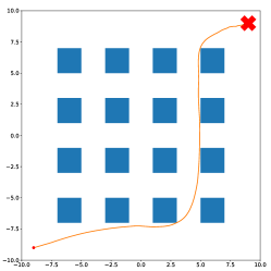
Refer to caption
Figure 5: Setup for the Planar Navigation task. The goal is for the robot (orange dot) to reach the goal location (red cross) while avoiding the obstacles (blue squares) in the middle. A crash cost of 100001000010000 is incurred for crashing into the obstacles.

We consider the task of navigating a 2D2𝐷2D double integrator through an obstacle field (see Fig. 5). The state consists of (xt,x˙t)subscript𝑥𝑡subscript˙𝑥𝑡(x_{t},\dot{x}_{t}), while the control is ut=xt¨subscript𝑢𝑡¨subscript𝑥𝑡u_{t}=\ddot{x_{t}}, where xt,x˙t,x¨t2subscript𝑥𝑡subscript˙𝑥𝑡subscript¨𝑥𝑡superscript2x_{t},\dot{x}_{t},\ddot{x}_{t}\in\mathbb{R}^{2} represent the position, velocity and acceleration of the system. For the initial position x0([99]T,[00]T)subscript𝑥0superscriptmatrix99Tsuperscriptmatrix00Tx_{0}\coloneqq(\begin{bmatrix}-9&-9\end{bmatrix}^{\mathrm{T}},\begin{bmatrix}0&0\end{bmatrix}^{\mathrm{T}}) and goal position xgoal([99]T,[00]T)subscript𝑥𝑔𝑜𝑎𝑙superscriptmatrix99Tsuperscriptmatrix00Tx_{goal}\coloneqq(\begin{bmatrix}9&9\end{bmatrix}^{\mathrm{T}},\begin{bmatrix}0&0\end{bmatrix}^{\mathrm{T}}), we defined the quadratic cost function:

J(X,U)=10000ccrash+(xTxgoal)TQf(xTxgoal)+t=0T1(xtxgoal)TQt(xtxgoal)+utTRut,𝐽𝑋𝑈10000subscript𝑐crashsuperscriptsubscript𝑥𝑇subscript𝑥goalTsubscript𝑄𝑓subscript𝑥𝑇subscript𝑥goalsuperscriptsubscript𝑡0𝑇1superscriptsubscript𝑥𝑡subscript𝑥goalTsubscript𝑄𝑡subscript𝑥𝑡subscript𝑥goalsuperscriptsubscript𝑢𝑡T𝑅subscript𝑢𝑡J(X,U)=10000c_{\text{crash}}+(x_{T}-x_{\text{goal}})^{\mathrm{T}}Q_{f}(x_{T}-x_{\text{goal}})+\sum_{t=0}^{T-1}(x_{t}-x_{\text{goal}})^{\mathrm{T}}Q_{t}(x_{t}-x_{\text{goal}})+u_{t}^{\mathrm{T}}Ru_{t}, (113)

where ccrashsubscript𝑐crashc_{\text{crash}} is the indicator variable for crashing into an obstacle, and

Qtsubscript𝑄𝑡\displaystyle Q_{t} diag([0.50.50.20.2])absentdiagmatrix0.50.50.20.2\displaystyle\coloneqq\operatorname{diag}(\begin{bmatrix}0.5&0.5&0.2&0.2\end{bmatrix}) (114)
QTsubscript𝑄𝑇\displaystyle Q_{T} diag([0.250.2511])absentdiagmatrix0.250.2511\displaystyle\coloneqq\operatorname{diag}(\begin{bmatrix}0.25&0.25&1&1\end{bmatrix}) (115)
R𝑅\displaystyle R diag([0.010.01]).absentdiagmatrix0.010.01\displaystyle\coloneqq\operatorname{diag}(\begin{bmatrix}0.01&0.01\end{bmatrix}). (116)

SM-4-B Quadrotor

The quadrotor task includes navigating a 3D obstacle course with 35 randomly placed obstacles while trying to reach a target location and hover. The control of the quadrotor is done through angular rates and a thrust command, we assume a low level tracking controller that is common for flight systems. The state of the quadrotor x𝑥x is composed of the 3 coordinates x,y,z𝑥𝑦𝑧x,y,z angular position represented in quaternions and linear and angular velocities for a total of 13 states. The location of target is represented in cartersian coordinates by xtargetsubscript𝑥𝑡𝑎𝑟𝑔𝑒𝑡x_{target} and is located at (25,25,5). The initial location x0subscript𝑥0x_{0} of the quadrotor is at (0,0,5). For this task, we use the following quadratic cost function:

J(X,U)=t=0T140xtargetx+10x˙+2ω+1e7ccrash,𝐽𝑋𝑈superscriptsubscript𝑡0𝑇140normsubscript𝑥𝑡𝑎𝑟𝑔𝑒𝑡𝑥10norm˙𝑥2norm𝜔1𝑒7subscript𝑐𝑐𝑟𝑎𝑠J(X,U)=\sum_{t=0}^{T-1}40\|x_{target}-x\|+10\|\dot{x}\|+2\|\omega\|+1e7c_{crash}, (117)

where x𝑥x is the cartesian coordinates of the quadrotor, x˙˙𝑥\dot{x} is the linear velocity, ω𝜔\omega is the angular rates, and ccrashsubscript𝑐𝑐𝑟𝑎𝑠c_{crash} is the indicator function that is 111 if the following conditions are met, and 00 otherwise

  1. 1.

    If the vehicle gets within 0.75 of an obstacle.

  2. 2.

    If the vehicle goes above 10 meters or below 0 meters in the z axis.

SM-4-C Franka

The Franka manipulator is modified to have 777-DOF by removing the last joint and fixing the fingers in place. For state x(e,e˙)𝑥𝑒˙𝑒x\coloneqq(e,\dot{e}) and control uq˙𝑢˙𝑞u\coloneqq\dot{q}, where e,e˙3𝑒˙𝑒superscript3e,\dot{e}\in\mathbb{R}^{3} are the position and velocity of the end-effector, and q˙7˙𝑞superscript7\dot{q}\in\mathbb{R}^{7} are the joint velocities, the objective is to reach the goal position xgoalsubscript𝑥goalx_{\text{goal}} with obstacles between the starting position of the end effector and the goal. For this task, we use the following quadratic cost function:

J(X,U)=t=0T15etxgoal+0.1e˙t.𝐽𝑋𝑈superscriptsubscript𝑡0𝑇15delimited-∥∥subscript𝑒𝑡subscript𝑥goal0.1delimited-∥∥subscript˙𝑒𝑡J(X,U)=\sum_{t=0}^{T-1}5\lVert e_{t}-x_{\text{goal}}\rVert+0.1\lVert\dot{e}_{t}\rVert. (118)

SM-4-D Ant

For the Ant, we take inspiration from the cost function for the HalfCheetah from [5] and modify the cost function to reward forward velocity. For the instantaneous x velocity vtsubscript𝑣𝑡v_{t}, torso height htsubscript𝑡h_{t} and angle to the vertical axis α𝛼\alpha, the cost function J𝐽J is defined as

J(X,U)=t=0T1vt𝟏{ht0.7}𝟏{|α|0.5}+0.005ut2.𝐽𝑋𝑈superscriptsubscript𝑡0𝑇1subscript𝑣𝑡subscript1subscript𝑡0.7subscript1𝛼0.50.005superscriptdelimited-∥∥subscript𝑢𝑡2J(X,U)=\sum_{t=0}^{T-1}-v_{t}\bm{1}_{\{h_{t}\leq 0.7\}}\bm{1}_{\{\lvert\alpha\rvert\geq 0.5\}}+0.005\lVert u_{t}\rVert^{2}. (119)

SM-4-E Humanoid

Similar to the Ant, we modify the cost function to reward forward velocity only if the height of the agent’s root is not too close or far from the ground and the humanoid is oriented upwards. For the instantaneous x velocity vtsubscript𝑣𝑡v_{t}, torso height htsubscript𝑡h_{t} and angle to the vertical axis α𝛼\alpha,

J(X,U)=t=0T1vt𝟏{0.85ht1.4}𝟏{|α|0.5}+0.005ut2.𝐽𝑋𝑈superscriptsubscript𝑡0𝑇1subscript𝑣𝑡subscript10.85subscript𝑡1.4subscript1𝛼0.50.005superscriptdelimited-∥∥subscript𝑢𝑡2J(X,U)=\sum_{t=0}^{T-1}-v_{t}\bm{1}_{\{0.85\leq h_{t}\leq 1.4\}}\bm{1}_{\{\lvert\alpha\rvert\geq 0.5\}}+0.005\lVert u_{t}\rVert^{2}. (120)
TABLE V: System parameters
Timestep
System
Noise
(xtsubscript𝑥𝑡absentx_{t}\in) (utsubscript𝑢𝑡absentu_{t}\in) (ΔΔ\Deltat) (σ𝜎\sigma)
Planar Navigation 300 100 4superscript4\mathbb{R}^{4} 2superscript2\mathbb{R}^{2} 0.010.010.01 1.01.01.0
Quadcopter 400 100 13superscript13\mathbb{R}^{13} 4superscript4\mathbb{R}^{4} 0.0150.0150.015 6.676.676.67
Franka 80 8 14superscript14\mathbb{R}^{14} 7superscript7\mathbb{R}^{7} 0.0050.0050.005 0.50.50.5
Ant 128 8 29superscript29\mathbb{R}^{29} 8superscript8\mathbb{R}^{8} 0.050.050.05 0.0050.0050.005
Humanoid 128 8 55superscript55\mathbb{R}^{55} 21superscript21\mathbb{R}^{21} 0.0330.0330.033 0.050.050.05
TABLE VI: Optimization Hyperparameters Per Dynamics
System Warmup Iterations Iterations per Timestep Number of Samples MPC Horizon T𝑇T
Planar Navigation 8 1 256 96
Quadcopter 64 1 1024 150
Franka 32 2 256 20
Ant 32 4 256 20
Humanoid 32 4 1024 20
TABLE VII: Hyperparameters for Unimodal Gaussian

SystemOptimizerNumber of Mixtures L𝐿Lλ1superscript𝜆1\lambda^{-1}Elite Fractionr𝑟r Planar NavigationMPPI4443.0513.0513.051 CEM4440.770.770.77 Tsallis4440.0360.0360.03633.29433.29433.294 QuadcopterMPPI4440.6500.6500.650 CEM4440.0150.0150.015 Tsallis4440.0100.0100.0101.0401.0401.040 FrankaMPPI44437.030 8937.0308937.030\,89 CEM4440.027 253 10.02725310.027\,253\,1 Tsallis4440.450.450.451.151.151.15 AntMPPI44416.942816.942816.9428 CEM4440.050.050.05 Tsallis4440.0240.0240.0245.05.05.0 HumanoidMPPI44465.220 904 334 656 5565.2209043346565565.220\,904\,334\,656\,55 CEM4440.012 840 730 283 384 2330.0128407302833842330.012\,840\,730\,283\,384\,233 Tsallis4440.036 912 542 032 967 3160.0369125420329673160.036\,912\,542\,032\,967\,3166.280 917 657 828 7226.2809176578287226.280\,917\,657\,828\,722

TABLE X: Hyperparameters for Stein Policy

SystemOptimizerNumber of Particles N𝑁N   Kernel Bandwidth Multiplier   λ1superscript𝜆1\lambda^{-1}Elite Fractionr𝑟r Planar NavigationMPPI8881.031.031.0371.271.271.2 CEM8880.4620.4620.4620.0230.0230.023 Tsallis8889.4449.4449.4440.3820.3820.3823.420 QuadcopterMPPI8882.8692.8692.8693.8293.8293.829 CEM88812.90212.90212.9020.0710.0710.071 Tsallis8882.322.322.320.0470.0470.0472.077 FrankaMPPI8882.568 642.568642.568\,6450.159650.159650.1596 CEM88811.188111.188111.18810.228 7330.2287330.228\,733 Tsallis8887.17.17.10.370.370.372.0 AntMPPI8886.682 7126.6827126.682\,7128.159 6748.1596748.159\,674 CEM8887.17.17.10.150.150.15 Tsallis8887.17.17.10.40.40.42.5 HumanoidMPPI1616169.157 033 311 343 4769.1570333113434769.157\,033\,311\,343\,47663.527 052 042 637 09563.52705204263709563.527\,052\,042\,637\,095 CEM16161614.816 129 955 170 15614.81612995517015614.816\,129\,955\,170\,1560.021 217 670 912 240 6380.0212176709122406380.021\,217\,670\,912\,240\,638 Tsallis1616166.06.06.00.10.10.13.0

SM-6 Additional Results

In this section we include the results of different framework’s sensitivity with respect to its hyperparpameters on the planar navigation example with fixed variance unimodal Gaussian policy in LABEL:tab:sensitity. We also include the cumulative cost comparison plots of the simulator systems. All plots in this section show error bars of ±1plus-or-minus1\pm 1 standard deviation of the cost.

: TABLE VIIISensitivity Results for hyperparameters on planar navigation example with fixed variance unimodal Gaussian policy. Tsallis mean variation results are bolded. Note that Tsallis hyperparameters demonstrate lower cost sensitivity when perturbed from their baseline values.

MPPI       CEM           Tsallis       λ𝜆\lambda       γ𝛾\gamma       γ𝛾\gamma        r𝑟r    MeanStdMeanStdMeanStdMeanStd +10%30294.443499.193499.193499.1935 557.0735557.0735\,557.071753.461753.461753.4628 806.3428806.3428\,806.34531.6128873.70572.90 Baseline30023.733644.073644.073644.0734 617.4734617.4734\,617.472523.342523.342523.3428 714.7028714.7028\,714.70570.2028714.70570.20 -10%30143.854273.514273.514273.5134 427.0634427.0634\,427.062654.512654.512654.5128 571.6428571.6428\,571.64591.3728535.40657.00 Mean Variation (%)0.656.656.656.651.081.081.0812.6612.66-12.660.090.09-0.09-1.53-0.047.85

Refer to caption
TABLE X: Unimodal Gaussian on Manipulator
Refer to caption
TABLE X: Gaussian Mixture on Manipulator
Refer to caption
TABLE X: Nonparametric Stein Policy on Manipulator
Refer to caption
TABLE X: Unimodal Gaussian on Ant
Refer to caption
TABLE X: Gaussian Mixture on Ant
Refer to caption
TABLE X: Nonparametric Stein Policy on Ant
Refer to caption
TABLE X: Unimodal Gaussian on Humanoid
Refer to caption
TABLE X: Gaussian Mixture on Humanoid
Refer to caption
TABLE X: Nonparametric Stein Policy on Humanoid