Weighted Prime Powers Truncation of the Asymptotic Expansion for the Logarithmic Integral: Properties and Applications.

Abstract.

Given the asymptotic expansion for the logarithmic integral $\int_{0}^{n}\frac{dt}{\ln(t)}$, obtained from repeated integration by parts until the expansion terms reach a minimum; approaching zero. Which determines a cut-off for the number of terms in the expansion and this truncation is a function of $n$. By dropping the minimization constraint and introducing a new variable $x$ for the number of expansion terms, consider the question: Where to truncate the asymptotic expansion for the logarithmic integral to equal the prime count function $\pi(n)$?. Although constructing this new truncation function requires using the non-trivial zeros $\rho$ of the Riemann zeta function. There exists a closed form approximation that does not utilize the zeros at all. From this, a new bound is obtained on the summation $\sum_{\rho}li(n^{\rho})$. Which is then compared to an equivalent form of the Schoenfeld bound derived for this same summation. Resulting in a proof that the Riemann Hypothesis is true.

Keywords. Logarithmic Integral, Lambert W Function, Riemann Zeta Function, Riemann Hypothesis, Schoenfeld Bound.

1. Introduction

After a chance, re-introduction to the asymptotic expansion for the logarithmic integral. A question arose: Where would the expansion have to be truncated so that it equals the prime count function $\pi(n)$? Answering this question, and following through on exploring others it will raise, shall be the focus of all that follows.

Beginning with a definition for the logarithmic integral, with a case including offset integration limits to account for the singularity, needed for numeric calculations:

Definition 1.1.

$li(n):=\int_{0}^{n}\frac{dt}{\ln(t)}=li(2)+\int_{2}^{n}\frac{dt}{\ln(t)}\approx 1.04516+\int_{2}^{n}\frac{dt}{\ln(t)}$

The dependent variable $n$ can be real-valued, the notation adopted here refers back to $\pi(n)$, where the input is generally taken as integer-valued. Being a non-elementary integral, one method of solution is to use repeated integration by parts to generate an asymptotic expansion. Given as follows:

Definition 1.2.

$\int_{0}^{n}\frac{dt}{\ln(t)}=\frac{n}{\ln(n)}\sum_{k=0}^{\lfloor x\rfloor-1}\frac{k!}{\ln^{k}(n)}+x!\int_{0}^{n}\frac{dt}{\ln^{x+1}(t)}$

Since this expansion diverges with increasing $x$, to best approximate $li(n)$, it’s truncated at the value of $x$ that minimizes the integral term. Which will generally not be integer valued, requiring the floor function for the summation to make sense; in addition to using $x!:=\Gamma(x+1)$. Although the method of constructing the expansion forces $x$ to be integral valued, minimization means it must be viewed as continuous when appearing in the integral term. A notion that is then extended to the summation. When $x$ isn’t integer valued, some authors have added a linear interpolating or fractional term for real $x$ to reduce the truncation error.

Stieltjes in [Ref17] calculated the minimizing truncation, the first two terms are $\tau=\tau(n)\approx\ln(n)-1/3$; all other terms are reciprocal powers of $\ln(n)$. Stieltjes’s paper, originally in French, was reviewed in van Boven et. al. [Ref3], where a fractional term is included, ”derived from a heuristic reasoning about the remainder” of the expansion.

Another instance of using a fractional term occurs in the appendix of Stoll & Demichael [Ref16], along with additional correction terms and error bounds. For reference that information, preserving their notation, is reproduced here; where they use $x$ as a general input variable, same as $n$ is used just above. Also, notationally, $\log(x):=\ln(x)$ and $L_{1}:=\log(x),L_{2}:=\log(\log(x)),\cdots,L_{j}:=\log(\log(\cdots\log(x)))$.

This summation begins to diverge at $k=\lfloor L_{1}\rfloor$ so we stop at $k=\lfloor L_{1}-1\rfloor$. The error is almost logarithmically linear between integer changes in $L_{1}$, but the envelope of the error is not symmetric:

$$li(x)\cong\frac{x}{L_{1}}\sum_{k=0}^{\lfloor L_{1}-1\rfloor}\dfrac{k!}{L_{1}^{k}}\enspace\Big{\{}+1.2/\sqrt{L_{1}},-0.6/\sqrt{L_{1}}$$

For significantly higher accuracy, $li(x)$ can be expressed as a finite sum with smaller, symmetric errors as

$$\begin{split}li(x)\cong&\frac{x}{L_{1}}\Big{(}\sum_{k=0}^{\lfloor L_{1}-1\rfloor}\dfrac{k!}{L_{1}^{k}}+\frac{(L_{1}-\lfloor L_{1}\rfloor)\lfloor L_{1}\rfloor!\enspace}{L_{1}^{\lfloor L_{1}\rfloor}}\Big{)}\\ &-\Big{(}\frac{300L_{1}^{3/2}}{359L_{1}^{2}+L_{2}L_{1}-3L_{3}+3}\Big{)}-\Big{(}\frac{\sin(2\pi L_{1})}{7/3L_{1}^{2}61(L_{1}-2)}\Big{)}.\end{split}$$

The remaining error is estimated to be $<\frac{23L_{2}^{2}}{(L_{1}^{2}+48L_{1})^{2}}$ for $x>113$.

Although there are small differences between all the expansions for $li(n)$ given so far; e.g. location of truncation point and when the floor is applied to the upper summation limit. These are minor enough that one can still infer properties relating them. The property needed here is the error bound applying to an expansion with only the fractional term $\frac{(L_{1}-\lfloor L_{1}\rfloor)\lfloor L_{1}\rfloor!\enspace}{L_{1}^{\lfloor L_{1}\rfloor}}$ added. Expecting that within the quoted range of error bounds from $\frac{1}{\sqrt{L_{1}}}$ to $\frac{23L_{2}^{2}}{(L_{1}^{2}+48L_{1})^{2}}\sim\frac{1}{L_{1}^{4}}$, is where the error for including only this fractional term exists. Using this to guide a computational investigation into the approximation error to $li(n)$ incurred by using and expansion of the form:

Definition 1.3.

$li(n;x):=\frac{n}{\ln(n)}\sum_{k=0}^{\lfloor x\rfloor-1}\frac{k!}{\ln^{k}(n)}+\frac{(x-\lfloor x\rfloor)\lfloor x\rfloor!\enspace n}{\ln^{\lfloor x\rfloor+1}(n)},\forall n>1$, and $x\geq 1$.

The $x$ in definition (1.3) can take values independent of $n$. But to approximate $li(n)$ by using the Stieltjes truncation gives $li(n;\tau)$, that now fixes $x$ as a function of $n$. Computation using the pracma package in R to compute $li(n)$, shows that $li(n;\tau)$ has an error bound of at least, $|li(n)-li(n;\tau)|<\frac{0.5}{\ln^{2}(n)},\forall n\geq e^{4/3}$. Where the restriction on $n$ is to keep the truncation $\tau$ from becoming negative. From here on, this error will be assumed implicitly anytime $li(n)$ is replaced by the asymptotic expansion with a linear interpolation term.

Definition (1.3), must be modified to restore the connection with the integral term in definition (1.2). As it’s the summation’s source, determining both form and number of terms by imposing a minimization constraint. It essentially builds the expansion, except for the fractional term, and is then dropped; being effectively zero at it’s minimum. To sufficiently generalize this situation to be of use later, the main definition going forward is:

Definition 1.4.

$li(n;x):=\frac{n}{\ln(n)}\sum_{k=0}^{\lfloor x\rfloor-1}\frac{k!}{\ln^{k}(n)}+\frac{(x-\lfloor x\rfloor)\lfloor x\rfloor!\enspace n}{\ln^{\lfloor x\rfloor+1}(n)},\enspace\forall n>1$ & $x\geq 1$, s.t. for some fixed $V\geq 0$ have that $x$ is defined by $V:=x!\int_{0}^{n}\frac{dt}{\ln^{x+1}(t)}$.

For a fixed $n$, choosing $x$ to minimize $V$ gives the $li(n;\tau)$ case, making $x$ solely a function of $n$. Definition (1.4) works by using $n$ and $V$ to determine $x$, where the source integral term is not part of the expansion as it is in definition (1.2). Now, even though $V\not\approx 0$, it’s not added to the expansion, it only determines the number of terms. Using this more general view of the asymptotic expansion for the logarithmic integral. Treat the interpolation formula of definition (1.4) as defining a continuous ‘asymptotic expansion variable’ $x$, with a constraint condition. Ultimately $V$ will be a function of $n$, so it’s not included in the notation $li(n;x)$.

The fractional term allows for the asymptotic expansion function $li(n;x)$ to be jointly continuous. Technically, this is only the logarithmic integral for one specific truncation point $x=\tau$, so that referring to it generally as such is an abuse of the name. Done, as always, with the intention to maintain simplicity.

The layout of this paper is as follows. Section 2 will define, prove the existence of, and examine the exact prime truncation. Section 3 will do the same for the average prime truncation. Section 4 will derive the asymptotic form approximating an average of the prime truncation function, and then a specific form for large values of n. Finally, section 5 closes with an application of these new truncation functions to bounds on the summation over the zeta functions non-trivial zeros, and then compare them to Schoenfeld’s bound. Finally showing that the Riemann Hypothesis is true.

2. Exact Prime Truncation

2.1.

Using definition (1.4) to re-express the question posed at the beginning of the introduction: Where to truncate $li(n;x)$ to equal $\pi(n)$? Is expressed in the following definition;

Definition 2.1.

Exact Prime Truncation Function: Let $x_{\pi}(n)$ be such that, $li(n;x_{\pi}(n))=\pi(n).$

Note that no value for $V$ has been given, leaving the constraint condition of definition (2.1) unfulfilled. Part of the investigation here is to find a suitable $V$ to constrain the integral term to give $x_{\pi}(n)$. The idea used to find such a value is to compute $x_{\pi}(n)$ directly, and then determine the appropriate $V$. But, this will not be solved till the next section, and apply to a variant of $x_{\pi}(n)$. From that point it will be shown how to construct a $V$ for definition (2.1) to also fulfill the requirements of definition (1.4). The task at hand is to determine what constraint on the source integral’s value achieves the desired truncation of the $li(n;x)$ function.

Using the programming language R, and prime counting function from the RcppAlgos package, the question posed above was computationally examined. Solving the equation in definition (2.1) for $x$, gives the exact prime truncation point $x_{\pi}(n)$, to obtain the prime count from the asymptotic expansion function of the logarithmic integral. The result has strong local variations in value, that can be viewed as an average variation about a steadily increasing function; shown in figure (1). Most variation about this average is in fact determined by the zeta-zeros of Riemann’s exact formula, as it is the same information contained within $\pi(n)$. Something to be verified later on; in addition to clarifying what is meant by average in this case. Now, presenting graphs of the truncation value $x_{\pi}=x_{\pi}(n)$ that satisfies definition (2.1).

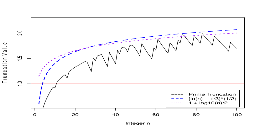
(a) Prime Truncation $x_{\pi}$ of $li(n),\ \forall n\in[2,100]$.

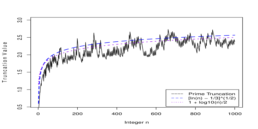
(b) Prime Truncation $x_{\pi}$ of $li(n),\ \forall n\in[2,1000]$.

Figure 1. Prime Truncation $x_{\pi}$ of $li(n)$.

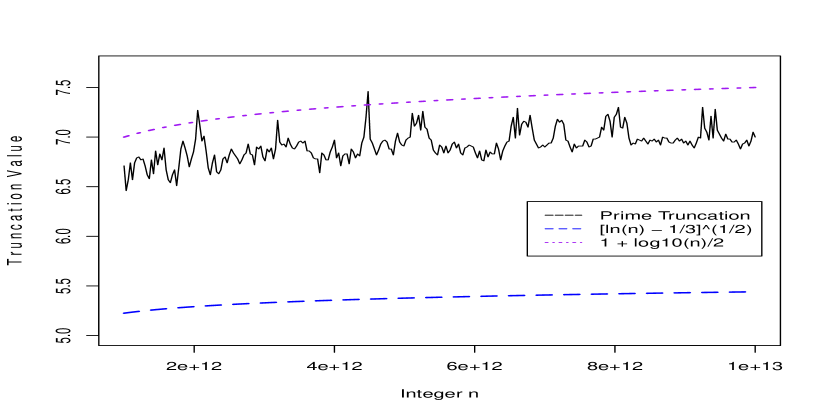
Figure 2. Prime Truncation $x_{\pi}$ of $li(n)$ such that $10^{12}\leq n\leq 10^{13}$.

The overall shape, seen in figures (1) &  (2) seems to possibly be derivable analytically, in part since it is fit well by the initial estimates $[\ln(n)-1/3]^{1/2}$ and $1+\log_{10}(n)/2$. Looking at figure (LABEL:PRIMETRUNC2TO100), can see that these functions miss the prime truncation function. Yet rather quickly assume something similar to an average for $n>100$, as seen in figure (LABEL:PRIMETRUNC2TO1000). The vertical line occurs at $n=11$, while the horizontal line is at a truncation value of $1$; signifying that the asymptotic expansion is undefined below this line, as cannot have less than one term, but is valid $\forall n\geq 11$. Altering the asymptotic expansion’s definition to allow the higher order terms to be subtractive to the initial term when $2\leq n<11$ provides a nice fit, since that is what’s shown in figure (LABEL:PRIMETRUNC2TO100); a bit more detail is given in second remark of Theorem 2.4. More investigation shows that $[\ln(n)-1/3]^{1/2}$ begins to fall short at about n $=10^{6}$, only becoming a worse fit for larger $n$; as seen in figure (2). After more examination, found $1+\log_{10}(n)/2$ to be a better fit up to about $n=10^{12}$; though it seems to surpass the mark as $n\rightarrow\infty$. Later on, will show why this function is so close to the average, and why it appears to exceed it.

Another feature to note is that the magnitude of the variation about what would be the average of the prime truncation is rather small to start, around $1/2$ and seems to decrease for $n>10^{12}$ to about $1/4$. The variations themselves are a direct consequence of the jumps and plateaus in the $\pi(n)$ function. Additionally, on a computational note, figure (1) displays all integer values in the specified ranges, while figure (2) only samples $301$ values.

Even though can compute such a solution for the equation in definition (2.1) up to $n\leq 10^{16}$, a proof is need $\for alln\geq 2$. Utilizing an analytical approach, such as that used by Axler [Ref1] and Dusart [Ref6] to prove various bounding inequalities for $\pi(n)$ shows the prime truncation solution always exists. In fact, these inequalities use specific truncations or alterations of the logarithmic integral’s asymptotic expansion. Which requires a specified range of applicability for the inequality, tying the truncation variable $x$ of the expansion to the input variable $n$. While generalizing this connection for such inequalities, and referencing Dusart’s work in  [Ref7] on similar inequalities. Axler in  [Ref1] packaged this idea into a functional form $g_{1}(x)$, taking integral values. E.g. Axler referenced Dusart obtaining the results, $g_{1}(2)=599$ & $g_{1}(3)=88,783$. Meaning that a 2-term expansion bounds $\pi(599)$, while a 3-term bounds $\pi(88,783)$.

Some notational differences to note from the referenced works. Use of the variables $n$ and $x$ is reversed, and the truncation $x_{\pi}$ in definition (2.1) is related to the inverse of $g_{1}(x)$, denoted here simply as $g(n)$; re-defined by the following:

Definition 2.2.

Let $g(n)$ be such that, $\pi(n)>li(n;g(n))=\frac{n}{\ln(n)}\sum_{k=0}^{g(n)-1}\dfrac{k!}{\ln^{k}(n)}.$

Although, a few values for $g(n)$ where given in relation to the inequalities discussed, no general form was shown or conjectured. Compared to the referenced examples, have $g(599)=2$ & $g(88,783)=3$; the actual computed values using the prime truncation are $x_{\pi}(599)=2.15$ & $x_{\pi}(88,783)=3.0$. Bringing Axler’s idea full circle; the same argument implies there exists a $G(n)$, essentially $1+g(n)$ for next tightest bound, that reverses the inequality in definition (2.2):

Definition 2.3.

Let $G(n)$ be such that, $\pi(n)<li(n;G(n))=\frac{n}{\ln(n)}\sum_{k=0}^{G(n)-1}\dfrac{k!}{\ln^{k}(n)}.$

Taken together, there must be an integral valued $g_{\pi}(n)$ such that:

(2.1) $$li(n;g(n))\leq\pi(n)\approx li(n;g_{\pi}(n))\leq li(n;G(n)).$$

Allowing $g_{\pi}(n)$ to be real-valued is the prime truncation $x_{\pi}(n)$ of the logarithmic integral; and the above equivalence can then be set to an equality. Note that since the exact solution will pass through integral values the inequalities have been change to include an equality condition. The linear interpolation term must also be added; since it is zero at integral values the original definitions are recovered. After searching all available references, Axler [Ref1] was the most explicit mention that is the closest to this idea. Proving the existence and uniqueness of such a function will use the basic method underlying the inequalities above.

Theorem 2.4.

(Prime Truncation) There exists, $\forall n\geq 11$, a unique continuous real-valued function $x_{\pi}(n)=g_{\pi}(n)$ such that;

(2.2) $$\pi(n)=li(n;g_{\pi}(n))$$

Proof.

By the prime number theorem $\pi(n)=li(n)+error(n)$; where the error is generally negative, except for Skewes regions where it must be positive. Normally, have no way to adjust $li(n)$, but introducing $li(n;x)$ allows for a fix. For some value of $x$ have that:

(2.3) $$\pi(n)=li(n)+error(n)=li(n;x)$$

By definition (2.1) $x=x_{\pi}$, which must be shown to exist and be unique. Where the idea is that by controlling the truncation point for the asymptotic expansion of $li(n)$ the target function $\pi(n)$ can be hit.

Consider the asymptotic expansion of $li(n)$ as defining a multiplicative correction factor $C(n,x)$ for $\frac{n}{\ln(n)}$. A view that comes from the asymptotic expansion function:

(2.4) $$li(n;x)=\frac{n}{\ln(n)}\sum_{k=0}^{x-1}\dfrac{k!}{\ln^{k}(n)}=\frac{n}{\ln(n)}(1+\frac{1}{\ln(n)}+\frac{2}{\ln^{2}(n)}+...)=\frac{n}{\ln(n)}C(n;x)$$

(2.5) $$C(n;x)=\sum_{k=0}^{x-1}\dfrac{k!}{\ln^{k}(n)}$$

The summation is Stieltjes form, used definition (1.4), denoted here by removing the floor on the upper summation limit; while also suppressing the fractional term, assuming it’s absorbed into the $C(n;x)$ function. Allowing for continuous adjustment of $\frac{n}{\ln(n)}$ by $C(n;x)$ through the asymptotic truncation variable $x$.

Have that $\frac{n}{\ln(n)}\leq\pi(n),\forall n\geq 11$, along with the fact that the correction factor $C(n,x)$ is a continuous monotonically increasing function $\geq 1$; since it’s a sum of positive terms. $C(n;x)$ also approaches infinity as $x$ does, because the asymptotic expansion is divergent. Giving a continuous range; $1\leq C(n,x)\leq\infty$. As $\frac{n}{\ln(n)}$ is a continuous monotonically increasing function, then so is $\frac{n}{\ln(n)}C(n;x)$.

For most $2\leq n<11$, it would require $C(n,x)<1$, which cannot happen with existing definition. When $n\approx 7$ again have $\frac{n}{\ln(n)}<\pi(n)$. Implying the need for a more complicated $C(n,x)$ when $2\leq n<11$; see the second remark following this proof for more elaboration.

Then $\forall n\geq 11$, since $\frac{n}{\ln(n)}\leq\pi(n)$, the correction $C(n;x)$ provides a continuous monotonic increase for $\frac{n}{\ln(n)}$ allowing $li(n;x)$ to meet then surpass $\pi(n)$; as the truncation variable $x$ increases. When $x=\tau$, the Stieltjes truncation, essentially have an equivalent form of the prime number theorem; $\pi(n)=li(n)+error(n)\approx li(n;\tau)+error(n)$. Since generally $error(n)<0$, the usual truncation $x=\tau$ must be cut short before $li(n;x)$ exceeds $\pi(n)$.

Since $\pi(n)$ is a piece-wise continuous, monotonically increasing step function. There must be a crossing point between $li(n;x)$ and $\pi(n)$ for some value of $x$, call it $x_{\pi}$; and by montonicity of both functions it must also be unique in the interval $[2,n]$. Embodied by the equality $C(n,x_{\pi})=\pi(n)\frac{\ln(n)}{n}$.

Therefore for all $n\geq 11$, a unique $x_{\pi}(n)=g_{\pi}(n)$ exists having the property that; $\pi(n)=li(n;g_{\pi}(n))$.

∎

Remark 2.5.

For Skewes regions where $li(n)>\pi(n)$; the theorem still holds, since have infinitely large correction factors $C(n,x)$ to choose from, these finite spikes can always be hit. Requiring a truncation past the usual Stieltjes point $\tau$, and into divergent territory of the asymptotic expansion.

Remark 2.6.

The Stieltjes Interpolation can be altered to allow for $0<C(n,x)<1$, when $2\leq n<11$; which actually works well in practice, again as it’s how the prime truncation $x_{\pi}$ is obtained for the figure (LABEL:PRIMETRUNC2TO100) plot in this range. I.e. subtracting terms of the form $\frac{k!}{\ln^{k}(n)},\ \forall k\geq 1$, from the initial $k=0$ term of $1$; representing a decrease in $\frac{n}{\ln(n)}$.

Remark 2.7.

The two notations $x_{\pi}$ and $g_{\pi}$ occur because $x$ was used to represent a specific truncation point for $li(n;x)$, before the work in Axler [Ref1] and Dusart [Ref7] was known. Where the $g$ notation from Axler and Dusart references a function that controls the number of terms in the asymptotic expansion for $li(n)$, that when allowed to take real values, coincides with $x_{\pi}$. From this point the $g$ notation will be used.

Although the prime truncation exists and is unique, solving for it requires knowing $\pi(n)$, or equivalently Riemann’s explicit formula and all the zeros of the zeta function; regardless of where they may lie. Making this function of interest, but not necessarily useful. Instead the remainder of this paper will focus on finding a closed form solution for it’s average behavior. Along with some applications.

3. Sum of Weighted Prime Powers & Its Relation to $g_{\pi}(n)$

3.1.

Riemann [Ref13] constructed an explicit formula for the prime count function $\pi(n)$, that was later proven by Mangoldt [Ref11], and others. Since then, a number of authors have studied and re-derived the formula; reproduced here from Dittrich [Ref5]. Having a slight symbol change of $Li$ to $li$ in the RHS summation; the source material defines $Li$ from $0$ to $n$; which makes better notational sense compared with $li$; i.e. an uppercase letter is larger than lowercase.

(3.1) $$\sum_{r=1}^{\lfloor\log_{2}(n)\rfloor}\dfrac{\pi(n^{1/r})}{r}=\int_{0}^{n}\frac{dt}{\ln(t)}-\sum_{\rho}^{zeta-zeros}li(n^{\rho})+\int_{n}^{\infty}\frac{dt}{(t^{2}-1)t\ln(t)}-\ln(2)$$

Where the summation over non-trivial zeros of the zeta function must be addressed. Questions concerning the Riemann Hypothesis (RH) now enter, regarding the zeros positioning in the complex plane. To be clear, the RH is not assumed. Everything that follows relies only on the validity of equation (3.1) and the fact that the non-trivial zeros are complex valued. Often, M$\ddot{o}$bius inversion is performed on equation (3.1) to obtain the final form used in practice, Kotnik [Ref10]. In this case the inversion is not needed, instead will work from equation (3.1). Also, note that the sum of weighted prime counts evaluated at the roots of $n$ will be referred to as the sum of weighted prime powers. Highlighting the terms source, rather than the term itself.

3.2.

For now, drop all but the logarithmic integral from the RHS of equation (3.1), and work with the equivalence:

(3.2) $$\sum_{r=1}^{\lfloor\log_{2}(n)\rfloor}\dfrac{\pi(n^{1/r})}{r}\approx\int_{0}^{n}\frac{dt}{\ln(t)}$$

Then separate out the first term of the summation on LHS of equation (3.2), while replacing RHS with its asymptotic expansion from definition (1.4), again suppressing the floor on the upper summation limit, denoting that fractional term is part of the sum. With the offset source integral added back to illustrate its connection to the sum of prime power counts.

(3.3) $$\pi(n)+\sum_{r=2}^{\lfloor\log_{2}(n)\rfloor}\dfrac{\pi(n^{1/r})}{r}\approx\frac{n}{\ln(n)}\sum_{k=0}^{x-1}\dfrac{k!}{\ln^{k}(n)}+x!\int_{2}^{n}\frac{dt}{\ln^{x+1}(t)}+li(2)$$

Essentially, by equating the first terms on each side and then the second terms. Have that the weighted sum of prime powers determines the source integral term, thus giving a truncation value when solving for $x$. Providing an idea on what the missing constraint in definition (2.1) should be. Now, by construction, the remaining expansion in this case is equivalent to $\pi(n)$. Requiring the next step of solving for $x$ in:

(3.4) $$\sum_{r=2}^{\lfloor\log_{2}(n)\rfloor}\dfrac{\pi(n^{1/r})}{r}=x!\int_{2}^{n}\frac{dt}{\ln^{x+1}(t)}+li(2)$$

This method does not seek to minimize the integral term, but set it to a specific value, correcting for the over-count error added to $\pi(n)$.

The LHS of equation (3.4) is the sum weighted prime power counts, and from this point on will refer to only powers $>1$. While the RHS of equation (3.4) will require multiple levels of approximation; e.g. moving to the asymptotic form of the integral and then approximating the inverse factorial. First, a computational investigation into the exact solution to equation (3.4) will be presented before delving into the approximating solution.

Using the prime count function in R to calculate the LHS of equation (3.4), and numeric integration for the RHS, then searching for $x$ values satisfying the equality. Produces the following series of graphs shown in figures (3), (4), & (5). These solutions are denoted by $\bar{g}_{\pi}(n)$, which will be referred to as the average prime truncation.

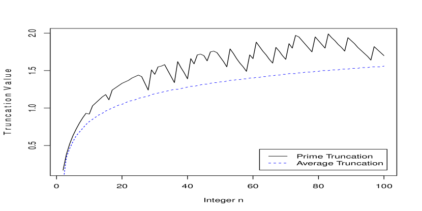
Figure 3. Prime $g_{\pi}(n)$ & Average Prime $\bar{g}_{\pi}(n)$ Truncation Functions; $2\leq n\leq 100$.

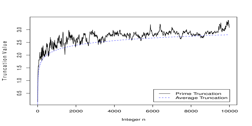
Figure 4. Prime $g_{\pi}(n)$ & Average Prime $\bar{g}_{\pi}(n)$ Truncation Functions; $2\leq n\leq 10^{4}$.

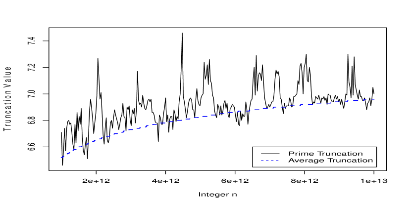
Figure 5. Prime $g_{\pi}(n)$ & Average Prime $\bar{g}_{\pi}(n)$ Truncation Functions; $10^{12}\leq n\leq 10^{13}$.

Notice how the solution follows closely what one would think is an averaging value of the prime truncation function. Here the basic notion of average for a continuous function is extended to a windowed or running average; defined by $average(f(x)):=\frac{1}{b_{x}-a_{x}}\int_{b_{x}}^{a_{x}}f(t)dt$, where the integration limits move with $x$, creating a window $[a_{x},b_{x}]$. In this case, e.g. a possible window would be $[x-1/2,x+1/2]$.

It does start a bit off, likely for two main reasons; its origin is from an equivalence after dropping terms from Riemann’s exact formula equation (3.1), and it relies on prime powers that take time to accumulate. Some computational errors do exist, mostly from numeric integration; e.g. “probably divergent” warnings and jumps in the minimum error. Mostly they are accurate, since extra code was added to check for the proper values; though it did increase run-time. Figure (3) plots all integral values in the given range, while figure (4) plots $1000$ values, and figure (5) plots $301$ values; and is just a close-up of the plot in figure (2).

This computationally verifies that the weighted prime powers determine an approximate average of the prime truncation function. Doing so by not minimizing the integral error term, as with the usual approach when computing $li(n)$, instead setting it equal to the error added to $\pi(n)$ by the over-count introduced from the weighted prime powers. Providing a value for the constraint $V$, that is determined by $n$.

Next, proving this computational verification by looking to Riemann’s equation (3.1). For clarity, will generally refer to $\bar{g}_{\pi}(n)$ as ’the average’ when really it’s just ’an average’, one of possibly many approximating $average(g_{\pi}(n)))$. Only set apart by being a consequence of the relation above involving the sum over weighted prime powers. Again, the averaging is meant in the context of smoothing out the jagged variation in the prime truncation function $g_{\pi}(n)$.

Definition 3.1.

(Average Prime Truncation Function) Let $x=\bar{g}_{\pi}(n)$ solve equation (3.4). I.e. $\bar{g}_{\pi}(n)$ is the truncation determined by the weighted sum of prime power counts as the constraint $V$ on the integral term in definition (1.4). So that;

(3.5) $$\sum_{r=2}^{\lfloor\log_{2}(n)\rfloor}\dfrac{\pi(n^{1/r})}{r}=\bar{g}_{\pi}(n)!\int_{2}^{n}\frac{dt}{\ln^{\bar{g}_{\pi}(n)+1}(t)}+li(2)$$

Next, to prove that $\bar{g}_{\pi}(n)$ behaves as it was computationally shown to in the above figures. While also relating back to $g_{\pi}(n)$, and explaining its variations seen in the figures up to this point. Moreover, it better clarifies the averaging behavior of the function.

Theorem 3.2.

(Average Prime Truncation) The function $\bar{g}_{\pi}(n)$ provides an initial approximation to the average behavior of ${g}_{\pi}(n)$, requiring no information from the non-trivial zeta zeros.

Proof.

Consider that any truncation can be viewed as splitting $li(n)$ into two functions at the truncation point $x$, a head and a tail such that; $li(n)\approx li(n;x)+[li(n;\tau)-li(n;x)]$. Using the truncation implied by equation (3.5), and letting $x=\bar{g}_{\pi}(n)$, then substituting into Riemmann’s equation (3.1).

(3.6) $$\begin{split}\pi(n)+\sum_{r=2}^{\lfloor\log_{2}(n)\rfloor}\dfrac{\pi(n^{1/r})}{r}&\approx li(n;\bar{g}_{\pi}(n))+[li(n;\tau)-li(n;\bar{g}_{\pi}(n))]\\ &-\sum_{\rho}^{zeta-zeros}li(n^{\rho})+\int_{n}^{\infty}\frac{dt}{(t^{2}-1)t\ln(t)}-\ln(2)\end{split}$$

Since, by construction, the prime powers sum on the LHS is equal to the tail function in square brackets on the RHS, they cancel. This tail is the ”error” determined by the source integral, which was set to the sum of weighted prime power counts. Leaving,

(3.7) $$\pi(n)-li(n;\bar{g}_{\pi}(n))\approx-\sum_{\rho}^{zeta-zeros}li(n^{\rho})+\int_{n}^{\infty}\frac{dt}{(t^{2}-1)t\ln(t)}-\ln(2)$$

As the constant and integral terms on the RHS provide diminishing and little influence over the zeros summation, the difference on the LHS must be predominantly controlled by the summation over non-trivial zeta function zeros. Whose oscillatory behavior is well known, shown specifically by Stoll & Demichael [Ref16] to be expressible as a summation in terms of cosines; or sines. When $n$ is considered to be a continuous variable it means that occasionally the LHS difference must be zero, giving an exact solution; the prime truncation from Theorem 2.4. Even though the integral and constant terms will give a small shift to where this zero occurs, it still will occur. In general the RHS summation term’s oscillation about $0$ both bounds and ultimately controls, the LHS difference.

By using the first few zeta-zeros can move some summation terms $li(n^{\rho})$ to modify the constraint $V=\sum_{r=2}^{\lfloor\log_{2}(n)\rfloor}\dfrac{\pi(n^{1/r})}{r}$. Now as more zeros are used, have a sequence of constraints and their related truncations, that move from $\bar{g}_{\pi}$ to $g_{\pi}$. So, $\bar{g}_{\pi}$ can be described as a baseline, or initial term, subject to corrections induced by $li(n^{\rho})$.

Therefore $\bar{g}_{\pi}(n)$ must be an approximation to the average behavior of $g_{\pi}(n)$, determined by equation (3.5); requiring no non-trivial zeta zeros.

∎

Remark 3.3.

The oscillation of the zeta zeros summation about zero requires that the average prime truncation $\bar{g}_{\pi}(n)$ periodically satisfy the definition of the prime truncation $g_{\pi}(n)$, and differ from it by an amount determined by the zeta zeros summation. This implies that given $g_{\pi}$ and then removing the oscillations, have $\bar{g}_{\pi}$ left over. From this; and with the aid of figures (3), (4), & (5); it can been seen that the use of ”average”, as described, is justified. Though possibly baseline or initial term would be better.

Equation (3.5) provides a path towards solving for the average behavior of the prime truncation function. Showing that the truncation point determined by using the proper constraint, $V$ as the sum of weighted prime powers, corresponds to ‘an averaging’ of the prime truncation function. Additionally, the proof shows, in a reverse of the direction used above, that a bound on the LHS difference would also apply to the summation over the zeta-zeros. After a final closed form asymptotic solution for $\bar{g}_{\pi}(n)$ is obtained, will return to this line of inquiry.

As the proof and remark show, using $V=\sum_{r=2}^{\lfloor\log_{2}(n)\rfloor}\dfrac{\pi(n^{1/r})}{r}+\sum_{\rho}^{zeta-zeros}li(n^{\rho})+\int_{n}^{\infty}\frac{dt}{(t^{2}-1)t\ln(t)}-\ln(2)$ to determine a truncation point for $li(n;x)$, gives $x=g_{\pi}(n)$. Fulfilling the constraint lacking in definition (2.1). Since the zeros of the zeta function are not needed to calculate the constraint to obtain $\bar{g}_{\pi}(n)$, this average will be the focus.

3.3.

Briefly looking a little more into how well $li(n;\bar{g}_{\pi}(n)$ approximates $\pi(n)$. Which is largely because $li(n;\bar{g}_{\pi}(n)$ closely approximates Riemann’s correction $R(n)$ for $li(n)$, defined next. Normally, the M$\ddot{o}$bius inversion of Riemann’s explicit equation (3.1), in part, produces a prime power correction function:

Definition 3.4.

(3.8) $$R(n)=\sum_{r=1}^{\lfloor\log_{2}(n)\rfloor}\dfrac{\mu(r)}{r}li(n^{1/r})$$

Whose extra terms work to correct the over count in $li(n)$ from the weighted prime powers. The same goal as $li(n;\bar{g}_{\pi}(n))$. Except $R(n)$ requires more computation on at least two levels; have many more terms to compute with all the instances of $li(n^{1/r})$, and the M$\ddot{o}$bius function’s cost.

A further consequence from the proof of Theorem 3.2, is that the function $li(n;\bar{g}_{\pi}(n))$ behaves a lot like $R(n)$. Below, in figures (6),  (7), &  (8), are a few graphs to show their relative behavior. Using the exact count $\pi(10^{27})$ from the On-Line Encyclopedia of Integer Sequences OEIS: A006880, to compare with the truncation $li(10^{27};\bar{g}_{\pi}(10^{27}))$, giving a relative error of $3.81\cdot 10^{-13}$ %. Compared to $li(10^{27})$ itself which has relative error of $1.64$ % to $\pi(10^{27})$, it’s a much better estimate with less calculation. While $R(10^{27})$ has relative error $1.05\cdot 10^{-13}$ %, nearly four times better than the truncated $li(10^{27})$ function, $li(10^{27};\bar{g}_{\pi}(10^{27}))$. This only adds to the evidence that they are approximately the same function.

As expected, $li(n;\bar{g}_{\pi}(n))$, starts a little off, before it better approximates $\pi(n)$; following from the same behavior of $\bar{g}_{\pi}(n)$. When comparing $R(n)$ and the truncated function $li(n;\bar{g}_{\pi}(n))$, they will generally alternate on which is a better fit to $\pi(n)$. Looking at figure (7), shows $li(n;\bar{g}_{\pi}(n))$ a better fit. While figure (8), shows that $R(n)$ is better; though not as good as $li(n;\bar{g}_{\pi}(n))$ was in the previous range, $R(n)$ can still achieve the same level of accuracy depending on chosen range examined. Overall will state, without proof, that $R(n)$ is the better approximation to $\pi(n)$; precisely how much so is the question.

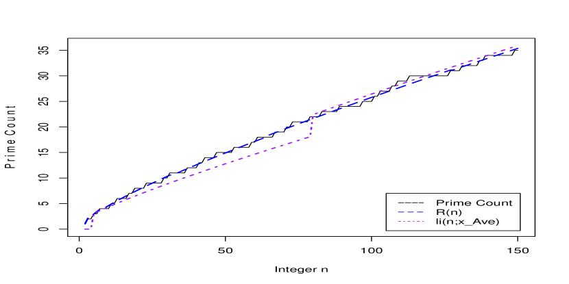
Figure 6. $\pi(n)$ vs. $R(n)$ vs. $li(n;\bar{g}_{\pi})\equiv li(n;x\_Ave);\forall n\in[2,150]$

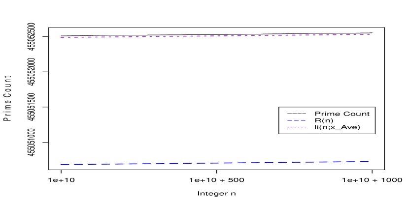
Figure 7. $\pi(n)$ vs. $R(n)$ vs. $li(n;\bar{g}_{\pi})\equiv li(n;x\_Ave);\forall n\in[10^{10},10^{10}+1000]$

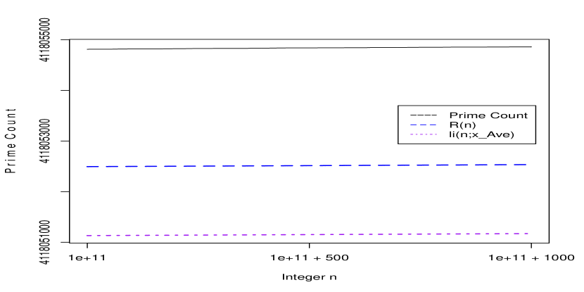
Figure 8. $\pi(n)$ vs. $R(n)$ vs. $li(n;\bar{g}_{\pi})\equiv li(n;x\_Ave);\forall n\in[10^{11},10^{11}+1000]$

4. Asymptotic Solution(s) To  $\sum_{r=2}^{\lfloor\log_{2}(n)\rfloor}\dfrac{\pi(n^{1/r})}{r}=\bar{g}_{\pi}(n)!\int_{0}^{n}\frac{dt}{\ln^{\bar{g}_{\pi}(n)+1}(t)}$

4.1.

The difficulties that arise when solving equation (3.4) are the following: 1) The RHS is a non-elementary anti-derivative. 2) Inverting the factorial function. 3) On LHS, require a means to generally calculate $\pi(n)$. 4) Obtaining a non-asymptotic solution for $x$ solely in terms of $n$; valid for all $n\geq 2$.

Focusing on the third issue for the moment. Up to this point have relied on sheer computational capacity to obtain $\pi(n)$ for up to $n=2^{53}<10^{16}$; currently not much better can be done, at least in a reasonable amount of time for the basic desktop PC tasked here. A Dell Optiplex 7040, with an I7-6700 cpu @3.4GHz and 16GB DDR4 RAM. Using a version the prime number theorem is the only recourse; falling again to the question of what degree of approximation. For the $\frac{n}{ln(n)}$ route, can bound via the asymptotic expansion of $li(n)$; as described above. Instead, using Riemann’s equation (3.1), or its M$\ddot{o}$bius inversion is a possibility, but would still have to mine infinitely many, or a great many, zeros of the zeta function.

A reasonable solution is to use the first few terms of $R(n)$. Normally, only the first two terms are used, since higher order terms are dominated by these two as well as the zeta-zero corrections. Still, to have good behavior for small $n$ as well, will use first five terms; i.e. up to first positive correction, occurring for $r=6$ in equation (3.8). Now, on to the other issues.

First, the anti-derivative can be replaced by its asymptotic approximation. Which is generally less than the integral for small $n$. With an error on the order of $O((x+1)!\ n/\ln^{x+2}(n))$; where $x$ is dependent on $n$.

Because the overall goal is to obtain an asymptotic form for the average prime truncation function, this approximation is valid. Although, its worthwhile to consider introducing a temporary multiplicative correction factor to remove any approximation. Defined by the ratio; where the tilde on $\tilde{\sigma}$ signifies its correcting for an integral:

(4.1) $$\tilde{\sigma}(n,x)=\frac{li(2)+\int_{2}^{n}\frac{dt}{\ln^{x+1}(t)}}{\frac{n}{\ln^{x+1}(n)}}$$

Implying a sigmoid-type correction , approaching $1$ as $n\rightarrow\infty$. Where sigmoid-type is meant to describe a generally monotonic function having two horizontal asymptotes. In this case, since concerned with increasing $n$, only require it to have one asymptote. This correction applies to small $n$, as it will essentially be set to $1$ for large $n$.

Noting that must input both an $n$ and its corresponding $x$ value to accurately check this function. Having to calculate the truncation value $x$, for each $n$, increases the complexity of the investigation into the precise asymptotic behavior of the integral in equation (3.5). Which is then further complicated by being tied to the prime count, causing this integral and its asymptotic form to fluctuate similarly as the other functions seen so far.

Approximating this ratio by a sigmoidal function will allow its product with the asymptotic form to fit the integral over a larger range; i.e. small $n$. With the correction dying off as the asymptotic equivalence is reached. The idea, only to undo some error from forced simplification of the integral for a more precise relationship.

Such a correction would be nice to have on its own, but introduced at this stage will over-complicate the solution. As it interferes with the method used to deal with both instances of the variable $x$, in the factorial and the exponent in the denominator

4.2. For General and Large $\mathbf{n}$

Next will need $W_{-1}(t)$ the lower branch of the Lambert $W$ function. Where $W(t)$ is the compositional inverse for the function $te^{t}$; making $W(t)$ something reminiscent of a logarithm. It takes two values on the negative real-axis, so is not actually a function, but by splitting into two branches, usually denoted $W_{0}$ and $W_{-1}$, single-valued functions are defined. The lower branch, $W_{-1}$, with domain $[-1/e,0)$; and tends back towards the y-axis from $t=-1/e$, taking only negative values.

Finally, an answer to the question posed at the introduction.

Theorem 4.1.

(Asymptotic Form of the Average Prime Truncation) Let $D_{n}$ be the density obtained from dividing the sum of weighted prime powers by $n$, then;

(4.2) $$\bar{g}_{\pi}(n)\sim\frac{\ln(D_{n})}{W_{-1}\Big{[}\frac{\ln(D_{n})}{e\ln(n)}\Big{]}}\enspace\forall n\geq 9$$

Proof.

Starting with equation (3.5), then moving to the asymptotic form of the integral $x!\int_{0}^{n}\frac{dt}{\ln^{x+1}(t)}\sim\frac{x!\ n}{\ln^{x+1}(n)}$ and dividing through by $n$; to obtain a density. Defined by the following;

(4.3) $$D_{n}:=\frac{1}{n}\sum_{r=2}^{\lfloor\log_{2}(n)\rfloor}\dfrac{\pi(n^{1/r})}{r}$$

Need to solve for $x$ in;

(4.4) $$D_{n}=\frac{x!}{\ln^{x+1}(n)}$$

Inverting the factorial function is only part of what is needed. The denominator’s exponent $(x+1)$ must also be dealt with. From Borwein et al [Ref2], a collection of results on the gamma function, showed that in Mumma [Ref12]:

(4.5) $$\lim_{x\rightarrow\infty}\frac{x!^{1/x}}{x}=\frac{1}{e}$$

Additionally, Borwein et al [Ref2] showed that the gamma function can be inverted via the Lambert $W$ function. Interesting, though not used here to directly solve for the factorial, the $W$ function still appears as a means of solution. Next, take the $x^{th}$ root of equation (4.4) then apply relation (4.5):

(4.6) $$D_{n}^{1/x}=\Big{[}\frac{x!}{\ln^{x+1}(n)}\Big{]}^{1/x}\approx\frac{x}{e\ln^{1+1/x}(n)}$$

Since $x$ increases with $n$, for large enough $n$, can assume $1/x\rightarrow 0$; at least much smaller than $1$. Gives a simplified form of equation (4.6) as:

(4.7) $$D_{n}\approx\Big{[}\frac{x}{e\ln(n)}\Big{]}^{x}$$

Using a particular case of a formula in Edwards [Ref8], after a substitution and rearrangement, provides the general solution, using the Lambert $W$ function’s lower branch, is given by:

(4.8) $$x=\frac{\ln(D_{n})}{W_{-1}\Big{[}\frac{\ln(D_{n})}{e\ln(n)}\Big{]}}$$

The details of the derivation are given in this paper’s appendix A1. Therefore, have that equation (4.8) gives an asymptotic solution to equation (3.5) for the average prime truncation function. Lastly, computation shows that for $4\leq n\leq 8$, the $W_{-1}$ function’s input causes it to be undefined for this range; otherwise it’s well-defined $\forall n\geq 9$.

∎

The overall form of function (4.2) fits with that of the prime truncation following a function of logarithmic type. Such as $[\ln(n)-1/3]^{1/2}$ or $1+log_{10}(n)/2$, for example. As the W function is like a logarithm, only growing slower, so then function (4.2) is like a logarithm divided by a weaker logarithm. Plots showing how this function behaves are seen in figures (9) &  (10).

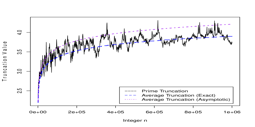
Figure 9. $g_{\pi}(n)$ vs. $\bar{g}_{\pi}(n)$ (Exact) vs. $\bar{g}_{\pi}(n)$ (Asymptotic); where $n\in[10^{3},10^{6}]$

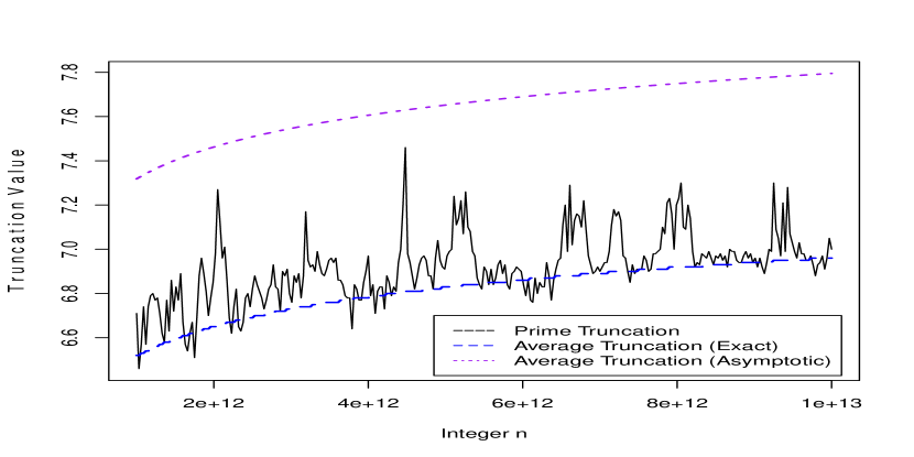
Figure 10. $g_{\pi}(n)$ vs. $\bar{g}_{\pi}(n)$ (Exact) vs. $\bar{g}_{\pi}(n)$ (Asymptotic); where $n\in[10^{12},10^{13}]$

In each figure the prime truncation is plotted along with an exact solution to equation (3.5) using a numerical approximation for the integral, and a solution to the simplified form of this equation that replaces the integral with its asymptotic form. Have already seen plots of the first two functions over the same or similar regions. Now, the asymptotic form can be seen to approximate the prime truncation rather well, but soon appears to grow beyond it. There are essentially three reasons for this behavior, all stemming from the three approximations that where made to obtain a nice functional form; equation (4.2). First the integral was simplified, next used an $x^{th}$-root and limit to simplify $x!$, then finally in the exponent of $\ln$, assumed that $(1+1/x)\rightarrow 1$ for large $n$. The influence of all simplifications diminish as $n$ increases, because $x$ increases along with it, though much slower being essentially logarithmicly related to $n$. The most important is the simplification of the integral, with the $\ln$ exponent being second, and the factorial being third.

Looking back at the sigmoidal correction $\tilde{\sigma}$ in equation (4.1). Examining this using the proper values of $n$ and its corresponding $x$, shows that the asymptotic form is less than the integral it approximates. At least to start with, then the ratio gradually approaches $1$. This is one reason why the plot of the average asymptotic form is larger than the exact solution $\bar{g}_{\pi}(n)$. Being a smaller function requires a larger $x$ value to hit the same mark. Figure (11) &  (12) below plots this sigmoid. Note that some spikes are likely small numeric integration errors, but generally the ratio’s nature is shown. There is a gradual downward trend, though rather erratic because of the variation carried over from the prime truncation.

Additionally, the exponent $1+1/x$ of $\ln$ having been replaced by $1$, means that the denominator involving this term will now be somewhat smaller that otherwise, increasing the ratio. This is largely why equation (4.2) starts off looking like a good fit, then veers off for larger $x$. It unintentionally compensates for the asymptotic form of the integral being smaller than the integral itself.

While the factorial correction is a minor influence by comparison, decreasing smoothly, taking values in the range $[1/e,1]$; when $x=5$, corresponding to $n\approx 10^{9}$, the ratio of limit relation (4.5) is $\approx 0.521034$, which is not too far from $1/e\approx 0.367879$. When $x=10$ the ratio is $\approx 0.4528729$, for $x=150$ it’s $\approx 0.3763755$. Showing a quick convergence on the $x$-scale; though rather slow on the $n$-scale.

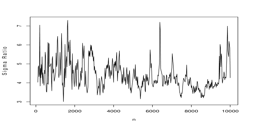
Figure 11. $\tilde{\sigma}(n,x_{\pi}),\ n\in[2,10^{5}]$

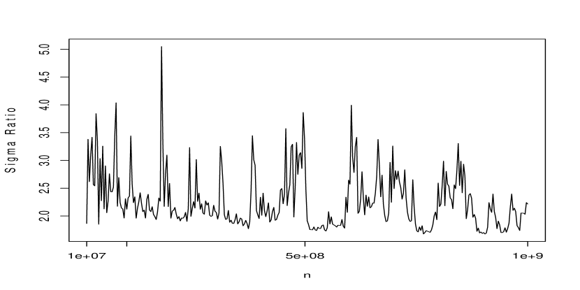
Figure 12. $\tilde{\sigma}(n,x_{\pi}),\ n\in[10^{6},10^{9}]$

Moving on to investigating the large $n$ behavior of function (4.2) by using the first order approximation $\frac{n}{\ln(n)}$ for the prime count function to simplify the following ratio, appearing as input to the $W$ function:

(4.9) $$\begin{split}\frac{\ln(D_{n})}{\ln(n)}&=\frac{\ln\bigg{(}\sum_{r=2}^{\lfloor\log_{2}(n)\rfloor}\dfrac{\pi(n^{1/r})}{r}\bigg{)}-\ln(n)}{\ln(n)}\\ &\approx\frac{\ln\bigg{(}\dfrac{1}{\ln(n)}\sum_{r=2}^{\lfloor\log_{2}(n)\rfloor}n^{1/r}\bigg{)}}{\ln(n)}-1\end{split}$$

In the limit as $n\rightarrow\infty$, using just the first term of the sum, this ratio approaches ${-1/2}^{-}$. Looking closer at the RHS of equation (4.9). Can essentially view the sum of successive roots of $n$ as follows:

(4.10) $$\sum_{r=2}^{\lfloor\log_{2}(n)\rfloor}n^{1/r}=n^{\beta_{n}},1/2\leq\beta_{n}\leq 1$$

Since the upper limit of the sum is an increasing function of $n$, the summation will grow in two ways with $n$. Though still not ultimately enough to dominate its main term and grow in any significant way.

Theorem 4.2.

Given $\beta_{n}$ from equation (4.10), then;

(4.11) $$\lim_{n\rightarrow\infty}\beta_{n}\rightarrow{1/2}^{+}$$

Proof.

Dividing equation (4.10) through by $n^{1/2}$ and simplifying:

(4.12) $$\sum_{r=2}^{\lfloor\log_{2}(n)\rfloor}n^{1/r-1/2}=1+\sum_{r=3}^{\lfloor\log_{2}(n)\rfloor}n^{\frac{-(r-2)}{2r}}=n^{\beta_{n}-1/2}$$

Where the sum of non-constant terms has the limit.

(4.13) $$\lim_{n\rightarrow\infty}\bigg{[}\sum_{r=3}^{\lfloor\log_{2}(n)\rfloor}n^{\frac{-(r-2)}{2r}}=\frac{1}{n^{1/6}}+\frac{1}{n^{1/4}}+\frac{1}{n^{3/10}}+...\bigg{]}\rightarrow 0^{+}$$

Being positive implies that beta takes values in the interval $[1/2,1]$. Leaving the following:

(4.14) $$\lim_{n\rightarrow\infty}n^{\beta_{n}-1/2}\rightarrow 1^{+}$$

This can only be true if the exponent of $n$ approaches $0$ from the right. All requiring beta to approach $1/2$ from the right. Therefore,

(4.15) $$\lim_{n\rightarrow\infty}\beta_{n}\rightarrow 1/2^{+}$$

∎

Using this with equation (4.9), have:

(4.16) $$\lim_{n\rightarrow\infty}\bigg{[}\frac{\ln(D_{n})}{\ln(n)}\approx\frac{\ln(n^{\beta_{n}})-\ln(\ln(n))}{\ln(n)}-1\bigg{]}\rightarrow\lim_{n\rightarrow\infty}\beta_{n}-1\rightarrow-1/2^{+}$$

So that inserting this result back into the Lambert $W$ gives:

(4.17) $$\lim_{n\rightarrow\infty}W_{-1}\bigg{[}\frac{\ln(D_{n})}{e\ln(n)}\bigg{]}\rightarrow W_{-1}\bigg{(}\frac{-1}{2e}\bigg{)}\approx-2.678347$$

Remarkably close to $-e$, which is a rather small, but important, change to the denominator in equation (4.2). After using a similar simplification on the numerator as in the denominator, seen in equation (4.16), have that up to a first-order approximation:

(4.18) $$\bar{g}_{\pi}(n)\approx\frac{(\beta_{n}-1)\ln(n)-\ln(\ln(n))}{W_{-1}\bigg{(}\frac{\beta_{n}-1}{e}\bigg{)}}$$

Combining the last few results with the simplified form in equation (4.18), allows for the following result.

Theorem 4.3.

The limit of the first order approximation to the asymptotic solution for the Average Prime Truncation Function $\bar{g}_{\pi}(n)$ has the following forms;

(4.19) $$\lim_{n\rightarrow\infty}\bar{g}_{\pi}(n)\rightarrow\tilde{g}_{\pi}(n)=0.186682\ln(n)$$

(4.20) $$\lim_{n\rightarrow\infty}\bar{g}_{\pi}(n)\rightarrow\tilde{g}_{\pi}(n)=0.186682\ln(n)+0.373365\ln(\ln(n))$$

Proof.

Proof: Using Theorem 4.2 and equation (4.17) in taking the limit of equation (4.18) as $n\rightarrow\infty$. Have;

(4.21) $$\lim_{n\rightarrow\infty}\bar{g}_{\pi}(n)\approx\frac{-\frac{1}{2}\ln(n)-\ln(\ln(n))}{-2.678347}\rightarrow\frac{\ln(n)}{5.356694}$$

Dividing through by $\ln(n)$, shows the limit approaches the constant $1/5.356694=0.186682$; since the $0.373365\ln(\ln(n))$ term is much smaller than $\ln(n)$ their ratio converges to $0$. Therefore, the given asymptotic form of the average prime truncation function approaches the stated limits, up to first order. ∎

Saying, “limit of asymptotic form”, not only means that equations (4.2),  (4.19) and  (4.20) are asymptotically equivalent; i.e. the limit of their ratio approaches $1$ as $n\rightarrow\infty$. Additionally, they are asymptotically equivalent to the exact solution for equation (3.5) that defines the average prime truncation. Where equation (4.2) is the more precise relation, over its simplified version, equation (4.20). Noting that this implies some analytical approximation is used for calculating the density $D_{n}$. Several options for doing so, having already been discussed. The simplest of which, a first-order approximation, was used to obtain the results just above, starting with equation (4.9).

Theorem 4.3 shows that the average prime truncation, as $n\rightarrow\infty$, is a little less than a fifth of the Stieltjes truncation for the logarithmic integral. Thus, have a better estimate of the prime count by using roughly the first one fifth of terms in the asymptotic expansion for the logarithmic integral. An estimate that parallels Riemann’s $R(n)$; partly shown in the proof of Theorem 3.2 and in the discussion that followed. Though now with less computational overhead than $R(n)$.

5. Connection to the Distribution of the non-Trivial Zeros for the Zeta Function.

5.1.

Returning to the line of inquiry which arose in Theorem 3.2, particularly equation (3.7), relating a summation over non-trivial zeros of the zeta function to a difference between the prime count $\pi(n)$ and the truncated logarithmic integral $li(n;\bar{g}_{\pi}(n))$. Any bound on this difference is then a bound on the summation. Since the truncated version is generally closer to the prime count than $li(n)$. It must be able to provide a tighter bound. With a possible exception for Skewes region’s, where $li(n)<\pi(n)$.

Again, the Riemann Hypothesis (RH) is not being assumed. The aim here is to see what bearing a tighter bound has, if any, on the non-trivial zeta-zeros positioning. So far nothing has relied on the position of the zeta function’s non-trivial zeros. Other than being complex valued and occurring in complex conjugate pairs; as used in the proof of Theorem 3.2.

The general idea for this section is to start from a new bound related to the difference $|\pi(n)-li(n)|$, that does not assume the RH to be true, separate $li(n)$ into two pieces via the average prime truncation point, and then simplify. Finally, apply this new bound to the zeros summation in equation (3.7), and compare to another bound equivalent to the RH.

To help simplify the argument, will refer to the two parts that $li(n)$ is split into as the truncated logarithmic integral and the remainder; same as that used in the proof of Theorem 3.2. Denoted by:

(5.1) $$li(n)\approx li(n;\bar{g}_{\pi})+[li(n;\tau)-li(n;\bar{g}_{\pi})]=li(n;\bar{g}_{\pi})+li_{R}(n;\bar{g}_{\pi})$$

Now, referring back to equation (3.7), reproduced here for convenience. Remembering that the remainder and weighted prime powers have been canceled out.

$$\pi(n)-li(n;\bar{g}_{\pi}(n))\approx-\sum_{\rho}^{zeta-zeros}li(n^{\rho})+\int_{n}^{\infty}\frac{dt}{(t^{2}-1)t\ln(t)}-\ln(2)$$

Require a suitable bound on the LHS difference. Dusart [Ref6] proved the following theorem, with table 1, bounding the Tchebyshev Theta function; defined as the following sum over prime $p$:

(5.2) $$\vartheta(n)=\sum_{\begin{subarray}{c}p\leq n\\ p\ prime\end{subarray}}\ln(p)$$

Theorem 5.2 [Dusart]: $\ \forall k\in\mathbb{N}_{0},\ \exists\eta_{k}$ and $n_{k}$, given in the following table 1, such that;

(5.3) $$|\vartheta-n|<\eta_{k}\frac{n}{\ln^{k}(n)},\forall n\geq n_{k}$$

Table 1. Dusart Theorem 5.2 Parameter Values

$$\begin{array}[b]{|c||c|c|c|c|c|c|c|}\hline\cr k&0&1&1&2&2&2&2\\ \hline\cr\eta_{k}&1&1.2323&0.001&3.965&0.2&0.05&0.01\\ \hline\cr n_{k}&1&2&908,994,923&2&3,594,641&122,568,683&7,713,133,853\\ \hline\cr\end{array}$$

$$\begin{array}[b]{|c||c|c|c|c|c|c|c|}\hline\cr k&3&3&3&3&4\\ \hline\cr\eta_{k}&20.83&10&1&0.78&1300\\ \hline\cr n_{k}&2&32,321&89,967,803&158,822,621&2\\ \hline\cr\end{array}$$

Where for each integral $k$ there are choices for the eta coefficient $\eta_{k}$ and the point $n_{k}$ at which the bound becomes valid. The tables show that several values for the coefficient $\eta_{k}$ can be chosen depending on the smallest allowed value $n_{k}$, for the input variable $n$. Or, the other way around, can choose a minimum $n_{k}$ and then find the associated $\eta_{k}$. Both assume a fixed $k$.

To apply this theorem, the first perspective shall be used. Along with choosing $\eta_{k}=(k-1)!$, which tends to be rather large, there will exist an $n_{k}$ , that should be rather small. From the tables, can see that a larger value for the input $n_{k}$ is required to decrease the $\eta_{k}$ coefficient’s value. Can interpolate and see for example that given $k=3$, have $\eta_{3}=2$, implying $32,321<n_{3}<89,976,803$. The exact value of $n_{k}$ does not matter, only its existence. While the choice for the $\eta_{k}$ coefficient is so that it matches a general term in the asymptotic expansion for $li(n)$.

Creating a key element to proving:

Theorem 5.1.

$|li(n;\bar{g}_{\pi})-\pi(n)|<\dfrac{n}{\ln(n)}\dfrac{(\bar{g}_{\pi}-1)!}{\ln(n)^{\bar{g}_{\pi}-1}},\forall n\geq n_{\bar{g}_{\pi}}$.

Proof.

Using the following identity between the prime counting function and Chebyshev’s function; Axler [Ref1]:

(5.4) $$\pi(n)=\frac{\vartheta(n)}{\ln(n)}+\int_{2}^{n}\frac{\vartheta(t)}{t\ln^{2}(t)}dt$$

Starting with a reverse of the difference that one usually encounters. Generally obtained by expanding $li(n)$ to first order, so that it has the same basic form as equation (5.4), then subtracting the prime count function. While also accounting for the constant term from the expansion, along with the slight offset between the definite integral in equation (5.4) and the one defining $li(n)$.

(5.5) $$li(n)-\pi(n)=\frac{n-\vartheta(n)}{\ln(n)}-\frac{2}{\ln(2)}+li(2)+\int_{2}^{n}\frac{t-\vartheta(t)}{t\ln^{2}(t)}dt$$

The two constant terms sum is approximately $-1.840226$, a small correction for large $n$. Next, using Theorem 5.2 [Dusart] can bound the two RHS non-constant terms. Applying the choice $\eta_{k}=(k-1)!$ for general exponents $k$, on the logarithm, there exists an $n_{k}$ such that:

(5.6) $$\frac{|n-\vartheta(n)|}{\ln(n)}<(k-1)!\frac{n}{\ln^{k}(n)}=\frac{n}{\ln(n)}\frac{(k-1)!}{\ln^{k-1}(n)},\forall n\geq n_{k}$$

(5.7) $$\int_{2}^{n}\frac{|t-\vartheta(t)|}{t\ln^{2}(t)}dt<(k-1)!\int_{2}^{n}\frac{dt}{\ln^{k+1}(t)},\forall n\geq n_{k}$$

Although the same index was used for inequalities (5.6) and  (5.7). This still will not yield the desired form for inequality (5.7). Want this to be of the same form as the source integral term in the expansion for $li(n;x)$. It’s very nearly there, just off by a factor of $k$. To fix this, only need to multiply through by $k$. Resulting in an appropriate inequality with the right form, given as:

(5.8) $$\int_{2}^{n}\frac{|t-\vartheta(t)|}{t\ln^{2}(t)}dt<(k-1)!\int_{2}^{n}\frac{dt}{\ln^{k+1}(t)}<k!\int_{2}^{n}\frac{dt}{\ln^{k+1}(t)},\forall n\geq n_{k}$$

Now, given equation (5.5), split $li(n)$ via equation (5.1), then apply inequalities (5.6) and  (5.8); dropping the constant $-2/\ln(2)$ term, and using the triangle inequality, finally rearranging to obtain:

(5.9) $$\begin{split}|li(n;\bar{g}_{\pi})-\pi(n)|&=\bigg{|}\frac{n-\vartheta(n)}{\ln(n)}-\frac{2}{\ln(2)}+li(2)+\int_{2}^{n}\frac{t-\vartheta(t)}{t\ln^{2}(t)}dt-li_{R}(n;\bar{g}_{\pi})\bigg{|}\\ &<\frac{|n-\vartheta(n)|}{\ln(n)}+\bigg{|}li(2)+\int_{2}^{n}\frac{|t-\vartheta(t)|}{t\ln^{2}(t)}dt-li_{R}(n;\bar{g}_{\pi})\bigg{|}\\ &<\frac{n}{\ln(n)}\frac{(k-1)!}{\ln^{k-1}(n)}+\bigg{|}li(2)+k!\int_{2}^{n}\frac{dt}{\ln^{k+1}(t)}-li_{R}(n;\bar{g}_{\pi})\bigg{|}\end{split}$$

Next step requires the index $k$ to be able to take real values. Nothing truly forces it to be integral. The only time it needs to be integral in Dusart [Ref6] is when it’s used to index the $k^{th}$ prime, but real values still make sense if the index is appropriately rounded. In fact the asymptotic expansion for the $k^{th}$ prime, and others, appear in the source paper. All view $k$ as real-valued.

Now that $k$ can take real values, set all instances of $k$ above to the average prime truncation function $\bar{g}_{\pi}(n)$. Then by construction, from equations (3.5) and  (3.6) used in the proof of Theorem 3.2, looking at the last line for equation (5.9) the RHS term in absolute value is zero. Giving the final inequality:

(5.10) $$|li(n;\bar{g}_{\pi})-\pi(n)|<\dfrac{n}{\ln(n)}\dfrac{(\bar{g}_{\pi}-1)!}{\ln(n)^{\bar{g}_{\pi}-1}},\forall n\geq n_{\bar{g}_{\pi}}$$

Where $n_{\bar{g}_{\pi}}$ also depends on which form of $\bar{g}_{\pi}$ is used. E.g. since the closed form involving the $W_{-1}$ function is valid $\forall n\geq 9$, in this case $n_{\bar{g}_{\pi}}=9$. For the other forms of $\bar{g}_{\pi}$ presented have $n_{\bar{g}_{\pi}}=2$. ∎

Remark 5.2.

Choosing $\eta_{k}=(k-1)!$ so freely is not an issue, since normally the name of the game is to make $\eta_{k}$ as small as possible. But, in this case it’s essentially the opposite and making $\eta_{k}$ larger doesn’t violate the inequality. Also, other choices can work, e.g. $\eta_{k}=(k-2)!$; giving a less tight bound; while the original $\eta_{k}=k!$ choice has some issues with determining where the bound holds, among others.

Independent of the RH, a bound on the zeta-zeros summation can now be expressed in the following theorem. Basically another corollary of Theorem 5.1.

Theorem 5.3.

(Truncation Bound)

(5.11) $$\bigg{|}\sum_{\rho}^{zeta-zeros}li(n^{\rho})\bigg{|}<\dfrac{n}{\ln(n)}\dfrac{(\bar{g}_{\pi}-1)!}{\ln^{\bar{g}_{\pi}-1}(n)}-0.553137,\ \forall n\geq n_{\bar{g}_{\pi}}$$

Proof.

Applying Theorem 5.1 to the RHS of equation (3.7):

(5.12) $$\bigg{|}-\sum_{\rho}^{zeta-zeros}li(n^{\rho})+\int_{n}^{\infty}\frac{dt}{(t^{2}-1)t\ln(t)}-\ln(2)\bigg{|}<\dfrac{n}{\ln(n)}\dfrac{(\bar{g}_{\pi}-1)!}{\ln^{\bar{g}_{\pi}-1}(n)}$$

The integral on the LHS is a decreasing function of $n$, its maximum occurring for $n=2$ is $0.140010$. Then subtracting the constant term $\ln(2)$ gives $0.140010-0.693147\approx-0.553137$; which will very quickly approach $-\ln(2)$ as $n$ increases. Combine these into a single constant. Since both remaining terms in absolute value are negative, can factor out and eliminate $-1$. Using the triangle inequality to obtain:

(5.13) $$\bigg{|}\sum_{\rho}^{zeta-zeros}li(n^{\rho})+0.553137\bigg{|}\leq\bigg{|}\sum_{\rho}^{zeta-zeros}li(n^{\rho})\bigg{|}+0.553137<\dfrac{n}{\ln(n)}\dfrac{(\bar{g}_{\pi}-1)!}{\ln^{\bar{g}_{\pi}-1}(n)}$$

Therefore, upon rearranging the constant term, the proof is complete.

∎

Next, need a bound equivalent to the RH. Turning to corollary $1$ of Theorem $10$ from Schoenfeld [Ref15], reproduced here.

Corollary 1 [Schoenfeld]: If the Riemann Hypothesis (RH) is true, then;

(5.14) $$|\pi(n)-li(n)|<\frac{n^{1/2}\ln(n)}{8\pi},\forall n\geq 2,657$$

Next, will use this bound to find a corresponding bound for the summation over the non-trivial zeta-zeros. Using equation (3.1), re-arrange to get the needed difference, then take the absolute value, then simplify using the triangle inequality:

(5.15) $$\begin{split}|\pi(n)-li(n)|&=\bigg{|}-\sum_{r=2}^{\lfloor\log_{2}(n)\rfloor}\frac{\pi(n^{1/r})}{r}-\sum_{\rho}^{zeta-zeros}li(n^{\rho})+\int_{n}^{\infty}\frac{dt}{(t^{2}-1)t\ln(t)}-\ln(2)\bigg{|}\\ &\approx\bigg{|}-\sum_{r=2}^{\lfloor\log_{2}(n)\rfloor}\frac{\pi(n^{1/r})}{r}-\sum_{\rho}^{zeta-zeros}li(n^{\rho})-0.553137\bigg{|}\\ &\geq\bigg{|}\sum_{\rho}^{zeta-zeros}li(n^{\rho})\bigg{|}-\sum_{r=2}^{\lfloor\log_{2}(n)\rfloor}\frac{\pi(n^{1/r})}{r}-0.553137\end{split}$$

As the negative constant term always dominates the positive integral term, can assume essentially have just three terms, all negative, in the first line. Seen when moving to the equivalence in the next line. Combining this with Corollary 1 [Schoenfeld], which is really just looking at other side of the equal sign, and though it does not explicitly appear in Schoenfeld [Ref15], will refer to as:

Corollary 1B [Schoenfeld]: If the RH is true, then;

(5.16) $$\bigg{|}\sum_{\rho}^{zeta-zeros}li(n^{\rho})\bigg{|}<\frac{n^{1/2}\ln(n)}{8\pi}+\sum_{r=2}^{\lfloor\log_{2}(n)\rfloor}\frac{\pi(n^{1/r})}{r}+0.553137,\forall n\geq 2,657$$

5.2.

To get a idea of the relationship between these two bounds on $|\sum_{\rho}^{zeta-zeros}li(n^{\rho})|$, will first use computational methods then prove some related results. Since the Truncation Bound of Theorem 5.3 can apply to the various approximations for the average prime truncation function $\bar{g}_{\pi}(n)$. The Truncation Bound’s behavior for two of these approximations is compared both to each other and to the related Schoenfeld bound. The exact form of $\bar{g}_{\pi}(n)$ computed from definition (3.1) gives the best case achievable. While the two limits $\tilde{g}_{\pi}(n)$ obtained from the closed form solution, are each worse case by comparison. Generally intend the more accurate limit $\tilde{g}_{\pi}(n)=0.186682\ln(n)+0.373365\ln(\ln(n))$, otherwise will mention when dropping the $\ln(\ln(n))$ term.

In figure (13) the solid black line is Schoenfeld’s Corrollary 1B bound on $|\sum_{\rho}^{zeta-zeros}li(n^{\rho})|$, while the other two lines are the Truncation Bounds with $\bar{g}_{\pi}(n)$ in dot-dash red, and $\tilde{g}_{\pi}(n)$ in dashed blue. The plot shows crossing points where each of the Truncation Bounds drop below the Schoenfeld bound. For the $\bar{g}_{\pi}(n)$ Truncation Bound have an intersection at $n\approx 6,062.860$, and for the $\tilde{g}_{\pi}(n)$ bound an intersection at $n\approx 33,519.932$. For comparison, when dropping $\ln(\ln(n))$ from the $\tilde{g}_{\pi}(n)$ Truncation Bound, now have a crossing at $n\approx 1.458\cdot 10^{12}$. A drastic change in the intersection point, but eventually both forms of $\tilde{g}_{\pi}(n)$ produce bounds that are less than the target bound of Schoenfeld.

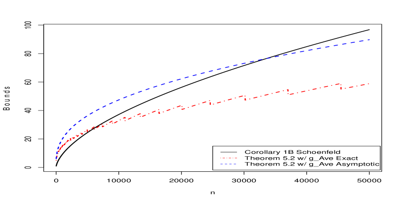
Figure 13. Corollary 1B [Schoenfeld] Vs. Theorem 5.3 w/ $\bar{g}_{\pi}(n)$ and $\tilde{g}_{\pi}(n)$, $\forall n\in[2,5\cdot 10^{4}]$

The question is now whether or not those relationships depicted in figure (13) extend to all $n>5*10^{4}$. Computations up to $n=10^{24}$ support the same ordering among all the bounds. Additionally, the distance between the two Truncation Bounds stays about the same, while their distance from the Schoenfeld bound only increases. These calculational assertions should be proven for the Truncation Bound using $\tilde{g}_{\pi}(n)$. Because $\bar{g}_{\pi}(n)$ is a computed object it cannot be used in such a proof, still it exists, and would fall under similar relations as $\tilde{g}_{\pi}(n)$. Such as the following theorem.

Theorem 5.4.

Let $\tilde{g}_{\pi}(n)=0.1866823\ln(n)$, then;

(5.17) $$\begin{split}|\sum_{\rho}^{zeta-zeros}li(n^{\rho})|&<\frac{n}{\ln(n)}\frac{(\tilde{g}_{\pi}-1)!}{\ln(n)^{\tilde{g}_{\pi}-1}}-0.553137\\ &<\frac{n^{1/2}\ln(n)}{8\pi}+\sum_{r=2}^{\lfloor\log_{2}(n)\rfloor}\frac{\pi(n^{1/r})}{r}+0.553137\ \forall n\geq 1.5\cdot 10^{12}\end{split}$$

Proof.

Let $\tilde{g}_{\pi}(n)=0.1866823\ln(n)$ using the simplest form available, and substitute into RHS of Theorem 5.3 to then define the function;

(5.18) $$f_{1}(n)\equiv\frac{n}{\ln(n)}\frac{(0.1866823\ln(n)-1)!}{\ln(n)^{0.1866823\ln(n)-1}}-0.553137$$

Also, have from Robbins [Ref14] there exists a variable $z$ such that;

(5.19) $$\sqrt{2\pi}z^{z+1/2}e^{-z}e^{\frac{1}{12z+1}}\leq z!\leq\sqrt{2\pi}z^{z+1/2}e^{-z}e^{\frac{1}{12z}},\ \forall z\in\mathbb{N}$$

On RHS take $z=1$ in $e^{\frac{1}{12z}}\Rightarrow e^{\frac{1}{12}}$ is max of this factor for all $z\geq 1$; and $\sqrt{2\pi}e^{\frac{1}{12}}\approx 2.724464$ is very close to $e$, just slightly larger; denote this new constant by $e^{+}$. From this, will use the inequality $z!\leq e^{+}z^{z+1/2}e^{-z}$ to bound $f_{1}$ from above and simplify by letting $z=0.1866823\ln(n)-1$;

(5.20) $$\begin{split}f_{1}(n)&\leq\frac{n}{\ln(n)}\frac{e^{+}[0.1866823\ln(n)-1]^{0.1866823\ln(n)-1+1/2}e^{-0.1866823\ln(n)+1}}{\ln(n)^{0.1866823\ln(n)-1}}-0.553137\\ &\leq\frac{n}{\ln(n)}\frac{e^{+}[0.1866823\ln(n)]^{0.1866823\ln(n)-1+1/2}e^{-0.1866823\ln(n)+1}}{\ln(n)^{0.1866823\ln(n)-1}}-0.553137\\ &=\frac{n}{\ln(n)}\frac{e^{+}e[0.1866823]^{0.1866823\ln(n)-1/2}\ln^{1/2}(n)}{n^{0.1866823}}-0.553137\\ &=n^{0.8133177}\frac{e^{+}e[0.1866823]^{0.1866823\ln(n)-1/2}}{\ln^{1/2}(n)}-0.553137\\ &=n^{0.8133177}\frac{e^{+}e(0.1866823)^{-1/2}[0.1866823^{0.1866823}]^{\ln(n)}}{\ln^{1/2}(n)}-0.553137\\ &=n^{0.8133177}\frac{17.14052\ [0.7310176]^{\ln(n)}}{\ln^{1/2}(n)}-0.553137,\ \forall n\geq 2\end{split}$$

Since the given inequalities on the factorial do not hold till $z\geq 1$, and have $z=0.1866823\ln(n)-1$, solving for $n$ implies requiring $n\geq 44,954$ (the actual value is $n\approx 44,953.71$). A closer check shows the inequality just derived actually holds $\forall n\geq 1.15$. Next let,

(5.21) $$f_{2}(n)\equiv\frac{n^{1/2}\ln(n)}{8\pi}+\sum_{r=2}^{\lfloor\log_{2}(n)\rfloor}\frac{\pi(n^{1/r})}{r}+0.553137$$

All terms are positive. Then have, by dropping last two terms; that $f_{2}(n)>\frac{n^{1/2}\ln(n)}{8\pi},\ \forall n\geq 2$.

To complete proof, must show that $f_{1}<f_{2},\ \forall n\geq n_{0}$; for some $n_{0}$. Combining the expressions for these two functions:

(5.22) $$\begin{split}f_{1}(n)&\leq n^{0.8133177}\frac{17.14052\ [0.7310176]^{\ln(n)}}{\ln^{1/2}(n)}-0.553137\\ &<\frac{n^{1/2}\ln(n)}{8\pi}<f_{2}(n)\end{split}$$

Rearranging the middle terms:

(5.23) $$\begin{split}[0.7310176]^{\ln(n)}&<\frac{n^{0.5-0.8133177}\ln^{3/2}(n)}{17.14052\cdot 8\pi}+\frac{0.553137\ n^{-0.8133177}\ln^{1/2}(n)}{17.14052}\\ &<\frac{n^{-0.3133177}\ln^{3/2}(n)}{17.14052\cdot 8\pi}\end{split}$$

Dropping the last term on the first line, as it decreases much faster than the other; e.g. $n=100$ has $100^{-0.3133177}\approx 0.2362461$ and $100^{-0.8133177}\approx 0.02362461$; and only grows smaller, somewhat quickly, for larger inputs. Taking the natural log of both sides gives:

(5.24) $$\ln(0.7310176)\ln(n)<-0.3133177\ln(n)+\frac{3}{2}\ln(\ln(n))-\ln(17.14052\cdot 8\pi)$$

Since $\ln(0.7310176)=-0.3133177$ the two logarithms on each side nicely cancel out, and calculating the RHS constant term, leaves:

(5.25) $$0<\frac{3}{2}\ln(\ln(n))-6.065617$$

Which is true $\forall n\geq e^{e^{6.065617/1.5}}\approx 5.915022\cdot 10^{24}$; and agrees with the computed intersection for the full inequality (5.23) at $n\approx 5.9144\cdot 10^{24}$. Additional computation using $f_{1}(n)$ and $f_{2}(n)$ puts the actual intersection at $n\approx 1.4579\cdot 10^{12}$, where the inequality has been computationally verified up to $n=10^{25}$. Therefore, have that the above string of inequalities hold, showing:

(5.26) $$f_{1}(n)<f_{2}(n),\ \forall n\geq 1.5\cdot 10^{12}$$

∎

Choosing the simplest form of $\tilde{g}_{\pi}(n)$ was to facilitate a cleaner proof. Using $\tilde{g}_{\pi}(n)=0.186682\ln(n)+0.373365\ln(\ln(n))$ in its place, or some suitable form of $\bar{g}_{\pi}(n)$, will produce similar theorems for these functions. They generally only differ on where the inequality’s validity begins. Referring back to figure (13) though not shown, the plot for the Truncation Bound using $\tilde{g}_{\pi}(n)=0.186682\ln(n)$ would be above that of $\tilde{g}_{\pi}(n)=0.186682\ln(n)+0.373365\ln(\ln(n))$ and $\bar{g}_{\pi}(n)$. Given that these functions are just a coarsening or refinement of each other, along with the supporting computations, the following theorems are also proven by Theorem 5.4.

Theorem 5.5.

Let $\tilde{g}_{\pi}(n)=0.1866823\ln(n)+0.373365\ln(\ln(n))$, then;

(5.27) $$\begin{split}|\sum_{\rho}^{zeta-zeros}li(n^{\rho})|&<\frac{n}{\ln(n)}\frac{(\tilde{g}_{\pi}-1)!}{\ln(n)^{\tilde{g}_{\pi}-1}}-0.553137\\ &<\frac{n^{1/2}\ln(n)}{8\pi}+\sum_{r=2}^{\lfloor\log_{2}(n)\rfloor}\frac{\pi(n^{1/r})}{r}+0.553137\ \forall n\geq 33,520\end{split}$$

Theorem 5.6.

Using the exact, computed form of $\bar{g}_{\pi}(n)$ then;

(5.28) $$\begin{split}|\sum_{\rho}^{zeta-zeros}li(n^{\rho})|&<\frac{n}{\ln(n)}\frac{(\bar{g}_{\pi}-1)!}{\ln(n)^{\bar{g}_{\pi}-1}}-0.553137\\ &<\frac{n^{1/2}\ln(n)}{8\pi}+\sum_{r=2}^{\lfloor\log_{2}(n)\rfloor}\frac{\pi(n^{1/r})}{r}+0.553137\ \forall n\geq 6,063\end{split}$$

Remark 5.7.

Even though the computed form of $\bar{g}_{\pi}(n)$ is used, it really shows that more accurate approximations for this function will approach this result. Improving their range of validity for smaller values of $n$, down to a minimum, providing tighter and tighter bounds.

5.3.

Though Corollary 1 [Schoenfeld] is stated as an implication, proving the bound true, independently of the RH, is equivalent to the RH being proven true. This bound is then equivalent to the Riemann Hypothesis. As would be any other sufficiently tight bound. Sufficient in the general sense defined by von Koch’s [Ref9] well known result; represented in modern form as:

(5.29) $$\lim_{n\rightarrow\infty}\pi(n)=li(n)+O(\sqrt{n}\ln(n))$$

Which can be recast in terms of the summation over the non-trivial zeros; just as Schoenfeld’s original bound was altered to obtain Corollary 1B [Schoenfeld] refocusing on $|\sum_{\rho}^{zeta-zeros}li(n^{\rho})|$.

Since Theorem 5.3 does not assume that the RH is true, and Corollary 1B [Schoenfeld] does assume it is true. If the Truncation Bound in Theorem 5.3 is less than or equal to the bound in Corollary 1B [Schoenfeld], then the RH must be true in general. Which is what Theorems 5.4, 5.5, and 5.6 all show. Finally drawing this section to a close by combining all previous results.

Theorem 5.8.

The Riemann Hypothesis is True.

Proof.

Given that the exact and average prime truncations of the asymptotic expansion for the logarithmic function exist; by Theorems 2.4 and  3.2. With their stated properties, the average truncation must provide a means to analyze the variations of the exact truncation; which are mostly due to the oscillatory behavior induced by the non-trivial zeta-zeros. Realized by using Riemann’s explicit equation (3.1) for the prime count function. By Theorems 4.1 and  4.3 there exists analytic solutions to the average truncation. Allowing for a new explicit bound, Theorem 5.3, on the zeta-zero summation term in equation (3.1), that does not assume anything about the location of those zeros. Again other than being complex-valued and occurring in complex conjugate pairs, to imbue the summation with real-valued sinusoidal properties.

Now, given that the Schoenfeld bound, when recast in terms of the zeta-zeros summation $|\sum_{\rho}^{zeta-zeros}li(n^{\rho})|$ , Corollary 1B [Schoenfeld], which does assume a condition on the location of the non-trivial zeros; i.e. that the RH is true. This bound is equivalent to the RH being true.

Next, considering the computational investigation shown above and Theorems 5.4, 5.5, and 5.6, have that the Theorem 5.3 Truncation Bound is less than the Corollary 1B [Schoenfeld] bound, for the given range, depending on which form of $\bar{g}_{\pi}(n)$ is used in the Truncation Bound. Thus, showing that a sufficiently tight bound is able to be constructed without assuming the RH; $\forall n\geq 6,064$ in the best case.

Since an equivalent to the Schoenfeld bound is beaten by the various Truncation Bounds, all without assuming the Riemann Hypothesis, then the RH must be true. Therefore, all non-trivial zeta-zeros $\rho$ are on the critical line $\Re(\rho)=1/2$.

∎

6. Conclusion

6.1.

As stated at the beginning of this paper, the goal was to answer a question about the asymptotic expansion of the logarithmic integral and explore its consequences. Leading to a verification that the Riemann Hypothesis is correct. This paper proceeded in the same way as the events of the discovery unfolded.

At first it seemed a truncated version of $li(n)$ would just provide a cheap computational short cut for a better approximation to $\pi(n)$, somewhat similar to Riemann’s $R(n)$. Which it does. Instead of calculating multiple instances of the $li(n)$ function with different inputs and combining them via $\mu(r)$ to compute $R(n)$; now just have to calculate about a fifth of the expansion for $li(n)$ and no $\mu(r)$.

But, the application of a truncation function to describe the variation induced by the zeta function’s non-trivial zeros turned out to be far more important. Essentially the main result follows from equating the weighted prime powers over-count to the “tail” or remainder of the logarithmic integral’s asymptotic expansion, and canceling them out. Which is equivalent, via Theorem 3.2, to the idea of the average prime truncation function. Additionally, gain a much tighter bound, Theorem 5.3, on the variation induced by the summation over the zeta-zeros than that provided by Schoenfeld’s equivalent bound on the same term.

Now having seen something of the average prime truncation function’s nature in relation to that of the prime truncation giving $\pi(n)$. It makes sense that it can bound the variation induced by the zeta functions non-trivial zeros so well. Effectively making the newly introduced asymptotic expansion variable $x$, akin to a type of logarithmic-like transform leading to an auxiliary function.

With a possible exception to this log-like transform. No new mathematics has really been introduced, which does make one feel like there is something not quite right. As with some problems, especially this one, it’s generally not only the expectation, but seemingly a necessity that new mathematics must arise to obtain a solution. With that in mind, the work here might best be characterized as using old mathematics by way of a new vantage point.

6.2. Future Work

Finding a better form of the average $\bar{g}_{\pi}(n)$; both in how well it fits the exact solution; i.e. no simplifications; and its ease of calculation. While another interesting route would be to determine how the $li(n^{\rho})$ terms in the zeta-zero summation map their corrections into the asymptotic domain of the truncation functions. Which can then be applied to $\bar{g}_{\pi}(n)$, by improving the constraint $V$ on the integral term, giving a better approximation to $g_{\pi}(n)$. Adding the integral and constant terms of Riemann’s explicit formula to the sum of prime powers constraint would be a small improvement. Further improving the competition between $li(n;\bar{g}_{\pi}(n)$ and $R(n)$.

Remark 6.1.

Consider a convenient notational modification: $\pi(n)\equiv$ $\pi$ $(n)$. Can view it as a symbolic bucket for placing primes $\leq n$.

APPENDIX

A1

Derivation of solution for linear exponential equation (4.8) from proof of Theorem 4.1. Equation & solution (23) reproduced, respectively, from Edwards [Ref8]:

(A-1) $$y=(ax^{b})^{cx^{d}}$$

(A-2) $$x=\frac{e^{\frac{W\big{(}\frac{a^{d/b}d}{bc}\ln(y)\big{)}}{d}}}{a^{1/b}}$$

Now, let $b=1$, $c=1$, and $d=1$, then have,

(A-3) $$y=(ax)^{x}$$

(A-4) $$x=\frac{e^{W(a\ln(y))}}{a}$$

If $a=1/(e\ln(n))$, then,

(A-5) $$x=e\ln(n)\ e^{W\big{(}\frac{\ln(y)}{e\ln(n)}\big{)}}$$

Still not the form needed, but close, since from one of the basic identities for the $W$ function derived directly from its definition is that;

(A-6) $$e^{W(z)}=\frac{z}{W(z)}$$

Using this identity with equation (A-5), have that;

(A-7) $$x=\frac{e\ln(n)\big{[}\frac{\ln(y)}{e\ \ln(n)}\big{]}}{W\big{(}\frac{\ln(y)}{e\ln(n)}\big{)}}=\frac{\ln(y)}{W\big{(}\frac{\ln(y)}{e\ln(n)}\big{)}}$$

Giving the correct form. Finally, setting $y=D_{n}$, the density provides the required solution.