Parallel two-scale finite element implementation of a system with varying microstructures

Abstract

We propose a two-scale finite element method designed for heterogeneous microstructures. Our approach exploits domain diffeomorphisms between the microscopic structures to gain computational efficiency. By using a conveniently constructed pullback operator, we are able to model the different microscopic domains as macroscopically dependent deformations of a reference domain. This allows for a relatively simple finite element framework to approximate the underlying PDE system with a parallel computational structure. We apply this technique to a model problem where we focus on transport in plant tissues. We illustrate the accuracy of the implementation with convergence benchmarks and show satisfactory parallelization speed-ups. We further highlight the effect of the heterogeneous microscopic structure on the output of the two-scale systems. Our implementation (publicly available on GitHub) builds on the deal.II FEM library. Application of this technique allows for an increased capacity of microscopic detail in multiscale modeling, while keeping running costs manageable.

Keywords

Multiscale modeling, varying microstructures, finite elements, computational efficiency

AMS subject classifications

65N30, 65N15, 35K58.

1 Introduction

Transport and diffusion phenomena interacting at multiple scales (multiscale) are ubiquitous in natural sciences and engineering [8]. Multiscale modeling is an effective technique to describe these phenomena, which may easily become computationally intractable. Specifically, scale-separated models allow us to examine the interplay between processes active on vastly different length and time scales; defining, for example, phenomena on macroscales and microscales [20, 45, 11]. Resolving microscale structures of heterogeneous nature is delicate as it requires a lot of computational effort, which left uncontrolled may have a devastating effect on scalability and run-times.

Here, we consider a flow process that takes place on two distinct physical scales. In the simplest setting, we can identify a macroscopic scale where a model governs the behavior of a (macroscopic) fluid in which averages over the microscopic scale enter as source terms, as well as a microscopic scale that includes diffusion-based transport and chemical reactions on heterogeneous domains where the macroscopic fluid concentration plays the role of a parameter. We propose a computational framework to model the effect of heterogeneous microscopic geometries on microscopic and macroscopic solution profiles, where the species involved satisfy a system of partial differential equations (PDEs). Resolving the multiscale structure of the PDEs, especially the heterogeneous microstructure, requires careful consideration to avoid computational overload yet make sure the required accuracy on the macroscale is achieved. We present an efficient and robust parallel two-scale finite element method for the approximation of such systems. Our focus in the present work is the consideration of linear systems of equations that preserve the main challenges that arise from the multiscale nature of the systems whilst sidestepping the added technical complications that arise in the nonlinear systems of more interest in applications. After showing that the model we consider is well-posed and that the finite element approximation we propose converges, we showcase the effects of the heterogeneous microstructures. In addition, we describe the different features of our framework, such as the capacity to run in parallel and the visualization of computational results.

As an example model to test the numerical method, we propose a system of PDEs describing the steady-state profile of transport processes in plants. The transport of many substances such as water, hormones and nutrients, occurs through cell scale processes. An important and widely studied example is that of Auxin transport [46], where active influx and efflux carriers on cell membranes allow for polarity of the transport process. Establishing and maintaining precise concentration profiles of Auxin in plant tissues is crucial in many developmental processes, making the problem inherently multiscale. Plant cells are orders of magnitude smaller than the size of the plant itself. Moreover, these cells vary greatly depending on plant age and location relative to the center of the stem. Taking these considerations into account can greatly complicate the process of developing a reliable computational model. In particular, using a single-scale model to resolve plant geometries in detail is extremely challenging from a computational point of view [46]. A number of recent studies focus on multiscale modeling with contributions ranging from modeling growing process [29, 22, e.g.]) to topological constructions [16, e.g.]. In [40] the author proposes a system of equations that models the consumption of water by plant roots and in [3, 7] the authors consider multiscale modeling of Auxin transport. The framework we develop is of relevance to all of these applications as our simulations of the linear model for transport in plant tissues show in Figure 4.

To the best of our knowledge, there are not many frameworks that treats scale-separated finite element formulations with heterogeneous microstructures. One of our aims is to provide researchers and practitioners with tools that help make problems like these computationally feasible. Moreover, the techniques presented in this manuscript are not limited to the applications described here. They can be flexibly extended to more complex multiscale problems, involving different kinds of physics such as coupling mechanics and fluid transport. One possible application is the modeling of cancer growth; an area where the need for multiscale models has been demonstrated [31].

Multiscale systems of equations have been studied extensively. Among some of the earlier contributions are [19, 44, 39]. A more recent overview of multiscale models can be found in for example [8] or [37].

Solving systems of PDEs, including multiscale ones, on complex geometries and with singular data often requires the use of unstructured grids or meshes. Owing to this, finite element approaches, known for their flexible use in complex geometries and relative ease in adaptive meshing, have received substantial attention for multiscale PDEs since the turn of the century. A review of concepts and advances can be found in [10]. Computational power has increased exponentially, but demands on model features and accuracy have managed to keep pace and use such power. Currently no single stratagem dominates the state-of-the-art.

It strongly depends in the problem at hand whether a given technique will prove effective or not. Rather than a single technique, multiscale modeling is a paradigm on how to relate said scales and make them interact. Multiscale models for PDEs can be classified in several different ways. One classification discriminates on whether the scales are physically embedded in each other or fully scale-separated [8, 37]. The first class thus formed allows for a size relation between a microscopic scale and a macroscopic scale and they must share spatial dimension; this class of models is studied, among others, by [17] and [9]. The second class, referred to as fully separate scale models, allows for different space dimensions at various scales, e.g., a one-dimensional microscopic domain within in a three-dimensional macroscopic domain. Our approach deals with this second class. Other examples of this technique can be found in for instance [36].

Multiscale models can also be classified in terms of how they encode patterns in microscopic structures. Techniques derived from homogenization often assume periodic (if not homogeneous) microscopic structures, as for instance demonstrated in [18] and [39]. This structure provides more tools for a rigorous mathematical analysis, but uses assumptions that are often too strong for practical applications. Since there is often an inherent variation present in microscopic structures, investigations such as [32, 21] focus on developing tools that allow for the modeling of that variation. Among the other contributions that focus specifically on varying or evolving microstructures are [1, 47, 25, 15].

Since a higher heterogeneity in the medium inevitably leads to more computational work, several contributions focus on improving computational strategies for multiscale simulations. Two of the most popular (and often-combined) approaches are employing adaptive grids for the discretization of the system of equations (adaptivity) and distributing the workload over different processors (parallelization): see for instance [14, 24] and [48]. In our framework, we apply a parallelization technique. For completeness, we mention that alternative solution approaches for multiscale flow and transport are studied as well, see [38, 39, 41, 30, e.g.].

The rest of the paper is structured as follows: in Section 2 we discuss the model PDE system and its analytic properties. In Section 3 we propose a finite element method and discuss its implementation. In Section 4 we report on numerical experiments conducted with this method and showcase the computational advantages with benchmarking and comparisons, including a parallel implementation and an application to test the dependence on the microscopic geometry. We close the paper with some conclusions.

2 A two-scale model with varying microstructures

Before posing the model problem, we introduce the two-scale setting and the heterogeneous microscopic structure. Let $\varOmega\subset\mathbb{R}^{d_{1}}$ be the macroscopic domain and $Y\subset\mathbb{R}^{d_{2}}$ be a microscopic domain with $d_{1},d_{2}\in\{1,2,3\}$. For each $x\in\varOmega$ we define a microscopic domain $Y_{x}\subset Y$. We denote the boundary of $\varOmega$ with $\partial\varOmega$, consisting of mutually disjoint parts $\partial\varOmega^{\mathrm{N}}$ and $\partial\varOmega^{\mathrm{D}}$ such that $\partial\varOmega=\partial\varOmega^{\mathrm{N}}\cup\partial\varOmega^{\mathrm{D}}$, and the boundary of $Y_{x}$ with $\varGamma_{x}$, consisting of mutually disjoint parts $\varGamma_{x}^{\text{I}}$ , $\varGamma_{x}^{\text{O}}$ and $\varGamma_{x}^{\text{N}}$, such that $\varGamma_{x}=\varGamma_{x}^{\text{I}}\cup\varGamma_{x}^{\text{O}}\cup\varGamma_{x}^{\text{N}}$. The different boundaries on the microscopic domain are presented in Figure 1. We proceed to define the composite (multiscale) domain $\varLambda$ as

$$\varLambda:=\bigcup_{x\in\varOmega}\{x\}\times Y_{x}.$$ (1)

Let $\zeta\in\operatorname{C}^{0}(\bar{\varOmega};\operatorname{C}^{1}(\bar{Z},\bar{Y}))$ be a mapping. Then, each of the microscopic domains $Y_{x}$ is constructed from a base domain $Z\subset Y$ as follows:

$$\zeta(x,Z)=Y_{x}.$$ (2)

Furthermore, assume that $\zeta(x,\cdot)$ is invertible for each $x$, that

$$c_{*}\leq\mathrm{det}\nabla_{y}\zeta(x,\cdot)\leq c^{*},$$ (3)

and that the partial inverse is smooth

$$\zeta_{y}^{-1}(x,\cdot):=\zeta^{-1}(x,\cdot):\operatorname{C}^{0}(\bar{\varOmega};\operatorname{C}^{1}(\bar{Y},\bar{Z})).$$ (4)

Similar setups of heterogeneous microscopic structures are presented in [32, 26, 47]. In continuum mechanics, this concept is often referred to as motion mapping [6]. See Figure 1 for a schematic representation of $\varOmega$ and $Y_{x}$. The boundary portions $\varGamma_{I}$, $\varGamma_{O}$ and $\varGamma_{N}$ represent the inflow, outflow and no-flow boundary of $Y_{x}$, respectively.

Figure 1: Schematic representation of the multiscale domain: at each macroscopic point $x\in\varOmega$ corresponds a microscopic domain $Y_{x}$ with mixed boundary conditions (pure Neumann or Robin).

2.1 Model problem

The following system of equations should primarily be regarded as a test problem for the two-scale finite element framework that is the main focus of this work. In order to illustrate the applicability of the framework, we describe an interpretation of the model as a description of transport processes in plants mediated by cell-scale influx and efflux. Under such an interpretation the macroscopic quantity $u$ represents a nutrient that the plant absorbs or produces, e.g., water absorbed from the soil. This nutrient is in turn taken in at cell membranes at an influx part of the membrane $\varGamma_{x}^{\text{I}}$, within the cells the nutrient concentration is represented by microscopic quantity $v$. In the cells, the nutrient $v$ is converted to a product $w$ which is emitted into the tissue at outflux regions of the cell membranes $\varGamma_{x}^{\text{O}}$. Such a description is consistent with simplifications of many models for Auxin and water transport in plants present in the literature [46, 7, e.g.]. As mentioned in the introduction, a major novelty of the model and the computational framework is that we allow for quite general cell geometries. In Figure 4 we illustrate the dependence of both macroscopic and microscopic solution profiles on the cell geometries.

Let $u,v:\varOmega\to\mathbb{R}$ and $v:\varLambda\to\mathbb{R}$ satisfy the following system of equations:

$$-\Delta_{x}u=f^{u}-\int_{\varGamma_{x}^{\text{I}}}\kappa_{1}u-\kappa_{2}v\operatorname{d}\!\sigma_{y} \mbox{ in }\varOmega,$$ (5)

$$u=u_{0} \mbox{ on }\partial\varOmega^{\mathrm{D}},$$

$$\nabla_{x}u\cdot n_{\varOmega}=0 \mbox{ on }\partial\varOmega^{\mathrm{N}},$$

$$-D^{v}\Delta_{y}v=f^{v} \mbox{ in }\varLambda,$$

$$D^{v}\nabla_{y}v\cdot n_{Y_{x}} =\begin{cases}\kappa_{1}u-\kappa_{2}v&\mbox{ on }\varGamma_{x}^{\text{I}}\\ \kappa_{3}w-\kappa_{4}v&\mbox{ on }\varGamma_{x}^{\text{O}}\\ 0&\mbox{ on }\varGamma_{x}^{\text{N}}\end{cases},$$

$$-\operatorname{div}\left(D^{w}\nabla_{x}w\right)=f^{w}-\int_{\varGamma_{x}^{\text{0}}}\kappa_{3}w-\kappa_{4}v\operatorname{d}\!\sigma_{y} \mbox{ in }\varOmega,$$

$$D^{w}\nabla_{x}w\cdot n_{\varOmega}=0 \mbox{ on }\partial\varOmega,$$

where $D^{w}\in\operatorname{L}^{\infty}(\varOmega)$, $u_{0}\in\operatorname{L}^{2}(\partial\varOmega^{\mathrm{D}})$ and $D^{v},\kappa_{1},\kappa_{2},\kappa_{3},\kappa_{4}\in\mathbb{R}$. In the rest of this manuscript, this system is referred to as (5). The function space $Q$ is defined as

$$Q:=\operatorname{H}^{1}_{\mathrm{D}}(\varOmega)\times\operatorname{L}^{2}\left(\varOmega;\operatorname{H}^{1}(Y_{x})\right)\times\operatorname{H}^{1}(\varOmega),$$ (6)

where $\operatorname{H}^{1}_{\mathrm{D}}(\varOmega)$ is the Sobolev space with Dirichlet values

$$\operatorname{H}^{1}_{\mathrm{D}}(\varOmega)=\left\{\phi\in\operatorname{H}^{1}(\varOmega)\middle|\phi|_{\partial\varOmega^{\mathrm{D}}}=0\right\}$$ (7)

and the slightly inconsistently denoted $\operatorname{L}^{2}(\varOmega,\operatorname{H}^{1}(Y_{x}))$ is rigorously defined as

$$\left\{\varphi\in\operatorname{L}^{2}(\varLambda):\exists\,\phi\in\operatorname{L}^{2}(\varOmega;\operatorname{H}^{1}(Z)):\varphi(x,\cdot)=\phi(x,\zeta^{-1}(x,\cdot))\text{ a.e. }x\in\varOmega\right\}.$$ (8)

We construct the weak form of (5) by multiplying the equations with test functions from the triplet $(\phi,\psi,\tilde{\phi})\in Q$ and integrating over the respective domains. This results in the following problem: find a triplet of functions $(u,v,w)\in Q$ such that

$$\begin{split}\int_{\varOmega}\nabla_{x}u\cdot\nabla_{x}\phi\operatorname{d}\!x&=\int_{\varOmega}\left(f^{u}-\int_{\varGamma_{x}^{\text{I}}}\kappa_{1}u-\kappa_{2}v\operatorname{d}\!\sigma_{y}\right)\phi\operatorname{d}\!x,\\ \int_{\varOmega}\int_{Y_{x}}D^{v}\nabla_{y}v\cdot\nabla_{y}\psi\operatorname{d}\!y\operatorname{d}\!x&=\int_{\varOmega}\int_{Y_{x}}f^{v}\psi\operatorname{d}\!y\operatorname{d}\!x+\int_{\varOmega}\int_{\varGamma_{x}^{\text{I}}}(\kappa_{1}u-\kappa_{2}v)\psi\operatorname{d}\!\sigma_{y}\operatorname{d}\!x\\ &+\int_{\varOmega}\int_{\varGamma_{x}^{\text{O}}}(\kappa_{3}w-\kappa_{4}v)\psi\operatorname{d}\!\sigma_{y}\operatorname{d}\!x,\\ \int_{\varOmega}D^{w}\nabla_{x}w\cdot\nabla_{x}\tilde{\phi}&=\int_{\varOmega}\left(f^{w}-\int_{\varGamma_{x}^{\text{O}}}\kappa_{3}w-\kappa_{4}v\operatorname{d}\!\sigma_{y}\right)\tilde{\phi}\operatorname{d}\!x,\end{split}$$ (9)

for all triplets of functions $(\phi,\psi,\tilde{\phi})\in Q$.

Definition 1.

We call the triplet $(u,v,w)\in Q$ a weak solution to (5) if it satisfies the identities listed in (9) for any choice of test functions $(\phi,\psi,\tilde{\phi})\in Q$.

2.2 Assumptions on data

Before proceeding with solvability of (5) we state the assumptions on which we base the proof:

1. $\varGamma_{x}^{\text{I}}\neq\emptyset$ and $\varGamma_{x}^{\text{O}}\neq\emptyset$ for all $x\in\varOmega$;

2. $\partial\varOmega^{\mathrm{D}}\neq\emptyset$;

3. $u_{0}\in\operatorname{L}^{2}(\partial\varOmega^{\mathrm{D}})$;

4. $D^{w}\in\operatorname{L}^{\infty}(\varOmega)$, $D^{w},D^{v}>0$, $f^{u},f^{w}\in\operatorname{L}^{2}(\varOmega)$ and $f^{v}\in\operatorname{L}^{2}(\varOmega;\operatorname{L}^{2}(Y_{x}))$;

5. $\kappa_{1},\dots,\kappa_{4}>0$;

6. We impose the following structural relations on the model parameters:

   $$\begin{split}\frac{|\kappa_{1}-\kappa_{2}|}{2}\left|\varGamma_{x}^{\text{I}}\right|&<1.\\ \frac{|\kappa_{3}-\kappa_{4}|}{2}\left|\varGamma_{x}^{\text{O}}\right|&<\min_{x\in\bar{\varOmega}}\{D^{w}(x)\}.\end{split}$$ (10)

Assumptions 1, 2 and 3 are geometric: they allow us to make sense of the function spaces with distributed microstructures without too many technicalities. Assumptions 4 and 5 have a clear physical translation. They point out a set of parameters for which solutions will turn to exist and to be unique. Assumption 6 is a sufficient condition to prove the coercivity of the bilinear form associated to (5), without being disrupted by the Robin boundary conditions. It reveals the physical interactions between the transmission coefficients $\kappa_{1},...,\kappa_{4}$, the size of the microstructure, and the macroscopic diffusion coefficient.

Theorem 1 (weak solvability).

Under assumptions 2.2.1–6 system (5) admits a unique solution in the sense of Definition 1 which is also stable with respect to parameters.

Proof.

Problem (5) is a linear and coupled system of elliptic equations. A standard application of the Lax–Milgram Lemma (cf. Theorem 1, on p. 317 in [12]) clarifies the solvability. A potentially less straightforward aspect is the structure of the function space $\operatorname{L}^{2}(\varOmega;\operatorname{H}^{1}(Y_{x}))$. Based on (A1) and (A2), and relying on [5], $\operatorname{L}^{2}(\varOmega;\operatorname{H}^{1}(Y_{x}))$ is a direct integral of Hilbert spaces, which is itself a Hilbert space together with its corresponding trace spaces $\operatorname{L}^{2}(\varOmega;\operatorname{L}^{2}(\varGamma_{x}^{\text{I}}))$ and $\operatorname{L}^{2}(\varOmega;\operatorname{L}^{2}(\varGamma_{x}^{\text{O}}))$. For more details on this topic, we refer the reader to [33] or to Section 2.2 in [32], which treats the topic of Sobolev spaces in non-cylindrical domains as used in this framework, as well as to the more recent account [13] for the $\operatorname{L}^{p}$ version of these spaces. ∎

3 Finite element implementation

3.1 Approximation

Rather than constructing a mesh for each of the microscopic domains $Y_{x}$, we use the structure in $\zeta(x,\cdot)$ to construct a mesh for the reference domain $Z$ only and pull-back the basis functions of $Y_{x}$ to $Z$. This leads us to mesh partition $\mathcal{B}_{H}$ for $\varOmega$ and mesh partition $\mathcal{K}_{h}$ for $Z$. From these meshes we construct the following macroscopic and microscopic finite element spaces:

$$U_{H} :=\left\{\left.u\in\operatorname{C}(\bar{\varOmega})\right|\,u|_{B}\in\mathbb{P}^{1}(B)\mbox{ for all }B\in\mathcal{B}_{H},\,u=0\mbox{ on }\partial\varOmega^{\mathrm{D}}\right\},$$ (11)

$$V_{h} :=\left\{\left.\hat{v}\in\operatorname{C}(\bar{Z})\right|\,\hat{v}|_{K}\in\mathbb{P}^{1}(K)\mbox{ for all }K\in\mathcal{K}_{h}\right\},$$

$$W_{H} :=\left\{\left.w\in\operatorname{C}(\bar{\varOmega})\right|\,w|_{B}\in\mathbb{P}^{1}(B)\mbox{ for all }B\in\mathcal{B}_{H}\ \right\}.$$

The multispace structure of the finite element space is inspired by constructions from [28, 36, 35].

Let $\mathcal{N}_{1}$ denote the set of degrees of freedom for $\mathcal{B}_{H}$. Let $\xi_{i}$ for $i\in\mathcal{N}_{1}$ denote a set of basis functions such that $W_{H}=\operatorname{span}(\xi_{i})$ and $U_{H}\subset\operatorname{span}(\xi_{i})$. Furthermore, let $\mathcal{N}_{2}$ denote the set of degrees of freedom for $\mathcal{K}_{h}$ and let $\hat{\eta_{j}}$ for $j\in\mathcal{N}_{2}$ denote a set of basis functions such that $V_{h}=\operatorname{span}(\hat{\eta_{j}})$. Note that we use hats on functions to indicate their correspondence to the reference domain $Z$. Now, approximating $(u,v,w)$ in the aforementioned finite element spaces yields:

$$u(x)=\sum_{i}\mathbf{u}_{i}\xi_{i}(x),\quad v(x,y)=\sum_{i,j}\mathbf{v}_{ij}\xi_{i}(x)(\zeta_{i}\circ\eta_{j})(y),\quad w=\sum_{i}\mathbf{w}_{i}\xi_{i},$$ (12)

In addition, we define the expressions

$$K(\cdot,y):=\left(\nabla_{y}\zeta(\cdot,y)\right)^{-1},$$ (13)

and

$$J(\cdot,y):=\det{\nabla_{y}\zeta(\cdot,y)},$$ (14)

to be able to express a function $v$ on $Y_{x}$ as a function of $\hat{v}$ on $Z$. Specifically, we make use of the transformations:

$$\int_{Y_{x}}v\operatorname{d}\!y= \int_{Z}vJ\operatorname{d}\!\hat{y},$$ (15)

$$\int_{Y_{x}}\nabla_{y}v\operatorname{d}\!y= \int_{Z}\nabla_{\hat{y}}\hat{v}KJ\operatorname{d}\!\hat{y},$$

$$\int_{\partial Y_{x}}\nabla_{y}v\cdot n_{y}\operatorname{d}\!\sigma_{y}= \int_{\partial Z}\nabla_{\hat{y}}\hat{v}\cdot KK^{T}n_{\hat{y}}J\operatorname{d}\!\sigma_{\hat{y}},$$

which hold almost everywhere on $\varOmega$ for any function $v\in\operatorname{L}^{2}(\varOmega;\operatorname{H}^{1}(Y_{x}))$.

Discretizing (9) and applying the transformations above we obtain a discrete weak formulation where the microscopic contributions only require reference cell $Z$:

$$\begin{split}&\sum_{i}\int_{\varOmega}\mathbf{u}_{i}\nabla_{x}\xi_{i}\nabla_{x}\xi_{k}\operatorname{d}\!x+\int_{\varOmega}\mathbf{u}_{i}\xi_{i}\xi_{k}\int_{\varGamma^{I}}\kappa_{1}J\operatorname{d}\!\sigma_{\hat{y}}\operatorname{d}\!x\\ &\quad=\int_{\varOmega}f^{u}-\left(\int_{\varGamma^{I}}(-\kappa_{2}\mathbf{v}J\operatorname{d}\!\sigma_{y}\right)\xi_{k}\operatorname{d}\!x,\\ &\sum_{i,j}\int_{\varOmega\times Z}\mathbf{v}_{ij}D^{v}\xi_{i}\nabla_{y}\hat{\eta_{j}}KK^{T}\nabla_{y}\hat{\eta_{l}}\xi_{k}Jd\hat{y}\operatorname{d}\!x+\int_{\varOmega\times\varGamma^{I}}\kappa_{2}\mathbf{v}_{ij}\xi_{i}\xi_{k}\hat{\eta_{j}}\hat{\eta_{l}}J\operatorname{d}\!\sigma_{\hat{y}}\operatorname{d}\!x\\ &\quad+\int_{\varOmega\times\varGamma^{O}}\kappa_{4}\mathbf{v}_{ij}\xi_{i}\xi_{k}\hat{\eta_{j}}\hat{\eta_{l}}J\operatorname{d}\!\sigma_{\hat{\eta_{l}}}\operatorname{d}\!x\\ &\quad=\int_{\varOmega\times Z}f^{v}\xi_{k}\hat{\eta_{l}}Jd\hat{y}\operatorname{d}\!x+\int_{\varOmega\times\varGamma^{I}}\kappa_{1}\mathbf{u}\xi_{k}\hat{\eta_{l}}J\operatorname{d}\!\sigma_{\hat{y}}\operatorname{d}\!x+\int_{\varOmega\times\varGamma^{O}}\kappa_{3}\mathbf{w}\xi_{k}\hat{\eta_{l}}J\operatorname{d}\!\sigma_{\hat{y}}\operatorname{d}\!x,\\ &\sum_{i}\int_{\varOmega}\mathbf{w}_{i}D^{w}\nabla_{x}\xi_{i}\nabla_{x}\xi_{k}+\int_{\varOmega}\mathbf{w}_{i}\xi_{i}\xi_{k}\int_{\varGamma^{O}}\kappa_{3}J\operatorname{d}\!\sigma_{\hat{y}}\\ &\quad=\int_{\varOmega}f^{w}-\left(\int_{\varGamma^{O}}-\kappa_{4}\mathbf{v}J\operatorname{d}\!\sigma_{\hat{y}}\right)\xi_{k}\operatorname{d}\!x.\end{split}$$ (16)

Using techniques similar to the ones presented in for instance [28], it is possible to prove a priori convergence rates of the finite element approximation. We do not provide such an analysis in this manuscript.

3.2 Implementation

We implement (16) using the finite element library deal.II [4], a C++ library that facilitates the creation and management of finite element implementations. The project is released under an open-source license and under active development. The choice for this library is motivated by its features, which include the possibility of dimension-independent implementations, support for many different elements and support for different parallelization options. Since deal.II does not directly support multiscale systems of PDE, we extend it with support for multiscale function and tensor objects. The implementation is available on GitHub [42].

3.3 Structure of FEM implementation

A classic finite element implementation in deal.II is roughly structured along the following steps:

1. Load a domain and generate a triangulation of that domain.

2. Distribute the degrees of freedom based on the triangulation and the degree of finite elements.

3. Initialize the system matrix and the right hand side and solution vector.

4. Assemble the linear system by looping over cells and integrate the discrete weak form for each quadrature point.

5. Apply the boundary conditions of the PDE to the linear system.

6. Precondition and solve the system, either directly or iteratively.

7. Post-process and output the solution.

In our finite element framework, we define a microscopic system for each macroscopic degree of freedom. More precisely, since we use basis functions with local support, the support point of the macroscopic basis function represents the location of the microscopic system. Correspondingly, we associate a specific local value of $u$ with each system: the finite element function value in the coordinates of the support point. This allows us to apply the same finite element framework for the microscopic functions over the macroscopic domains, creating in essence a tensor product of finite element spaces. The system is solved by decoupling the microscopic and macroscopic formulation. Iteratively, we solve first the macroscopic system, using the microscopic solutions of the previous iterations as data, followed by solving the microscopic system, using the most recently obtained macroscopic as data. We do so until we observe the difference between subsequent residuals is within a predetermined tolerance.

From a computational point of view, the effort associated with the creation and solving of microscopic systems can quickly become large. Applications that require solutions with high accuracies place demands on both memory and CPU capacity. For this reason, we address the computational load by customizing the implementation for multiscale systems using caching techniques, domain mappings, multithreaded assembly and distributed solving. Furthermore, we exploit the similarity between the different microscopic scales by using the same data structures for the microscopic systems, where possible.

3.4 Domain mappings

Mapping $\zeta$ is, as described in Section 2 implemented as a bounded, not necessarily linear function of both $x$ and $y$. $\zeta$ is supplied symbolically to the implementation, as well as the inverse of the Jacobian $K(x,y)$ (see (13)) We avoid recomputing these quantities by computing the structures $J$ and $KK^{T}J$ for each quadrature point and storing them in a hashmap for fast access throughout the iterative assembly procedure. Additionally, we apply the mapping in the multiscale functions, so that by using the same assembly objects for each $x$, we can evaluate all microscopic data on $Y_{x}$.

3.5 Parallelization in assembly

As mentioned before, we parallelize the implementation using multithreading. We divide computational the work into different threads which are assigned to processors that share memory, meaning that there is no need to specify communication between processors but that special care is needed to avoid so-called ’race conditions’, where errors are made due to multiple threads writing to the same memory structure at the same time, or one memory structure reading from the memory while another one is updating it.

A commonly used alternative is a distributed memory approach (based on for instance a message passing interface like MPI) where memory is distributed. This has the advantage of being able to be run on clusters of computing nodes that do not share a memory space, but has the disadvantage that data needs to be communicated explicitly and that often leads to communication overhead and idle time when a processor on a node is unused. The advantages of using a multithreading approach is that our settings lends itself well for doing so; there is minimal setup and overhead involved in the parallelization and the multiscale nature of the implementation reveals a structure that lends itself well for threads. A disadvantage is that most larger high performance clusters are composed of smaller compute nodes, requiring some sort of message passing. However, we remark that using a combination of multithreading and MPI is a valid strategy as well and something that could be applied on this setup too, as we discuss in Section 5.

We implement a multithreading approach using the Threading Building Blocks library, for which deal.II has integrations in place. In the assembly loop, we loop over all cells in reference domain $Z$ to compute the contributions of the associated degrees of freedom to the system matrix and the system right hand side vector. Rather than consecutively looping over all cells per microscopic system, we compute the contributions of all cells that correspond to the cell in the reference domain and add them to their respective system matrices. We use a thread-pool that assigns a new cell to a processor as soon as that processor has finished work on its previous cell, since all microscopic systems can be assembled independently. The result of this assembly step is a linear system for each microscopic finite element formulation. Both the macroscopic and microscopic systems are assembled in parallel, with a per-cell approach. This process can be run in parallel, since computing the contribution to the system matrix and the system right hand side of one finite element cell does not require information from other cells. This yields a linear system for each microscopic formulation.

The residual threshold used in this framework is the sum of the macroscopic and average microscopic residuals. The solution procedure is standard: we use the conjugate gradient method to solve the systems. The systems are also solved in parallel, by distributing them over the available processors.

3.6 Visualization

One of the most important post-processing steps of a simulation is visualizing the results. We make use of the visualization toolbox ParaView [2] and the associated library VTK [43]. The multiscale nature of the problem creates non-standard demands for the visualizations. In particular, since we solve the microscopic systems on the same reference domain, visualizing all of them at once is no longer a trivial task.

We need to push-forward the solution to the correct domain $Y_{x}$, since the microscopic systems are solved on $Z$. deal.II outputs data in a VTK-compliant format: an unstructured grid format ([43]). By applying the mapping on the transformation, we obtain a visual representation of the solution on the correct domain. In addition, we apply a translation to the microscopic unit domains to move them to their macroscopic location and scale for visualization purposes. Finally, ParaView can read these data files and render a visualization that provides an intuitive overview of the domain. The solutions to (5) are visualized using this technique and displayed in Figures 10 and 10.

4 Numerical experiments

We test and benchmark the implementation by applying the method of manufactured solutions on a system of PDE that generalizes (5). This allows us to see if our numerical scheme converges with the desired order, by prescribing a solution and deriving the corresponding PDE data. The manufactured system is formulated as follows:

$$-\Delta u =-\int_{\varGamma_{x}^{\text{I}}}\kappa_{1}u-\kappa_{2}v+g_{1}^{v}\operatorname{d}\!\sigma_{y}+f^{u} \mbox{ in }\varOmega,$$ (17)

$$u =u_{0}+g^{u}_{1} \mbox{ on }\partial\varOmega^{\mathrm{D}},$$

$$\nabla u\cdot n_{\varOmega} =g^{u}_{2} \mbox{ on }\partial\varOmega^{\mathrm{N}},$$

$$-D^{v}\Delta v =f^{v} \mbox{ in }\varLambda,$$

$$D^{v}\nabla_{y}v\cdot n_{Y_{x}} =\begin{cases}\kappa_{1}u-\kappa_{2}v+g^{v}_{1}\\ \kappa_{3}w-\kappa_{4}v+g^{v}_{2}\\ g^{v}_{3}\end{cases} \begin{matrix}\mbox{on }\varGamma_{x}^{\text{I}},\\ \mbox{on }\varGamma_{x}^{\text{O}},\\ \mbox{on }\varGamma_{x}^{\text{N}},\end{matrix}$$

$$-\operatorname{div}\left(D^{w}\nabla w\right) =-\int_{\varGamma_{x}^{\text{O}}}\kappa_{3}w-\kappa_{4}v+g_{2}^{v}\operatorname{d}\!\sigma_{y}+f^{w} \mbox{ in }\varOmega,$$

$$D^{w}\nabla w\cdot n_{\varOmega} =g^{w} \mbox{ on }\partial\varOmega.$$

4.1 SymPy

To facilitate the testing and benchmarking of the implementation, we build an interface that given a pair of manufactured solutions $(u,v)$ and a mapping $\zeta$ constructs the data of (17). This interface uses the symbolic algebra package SymPy [34] and outputs all required functions in a deal.II-compliant parameter file. This has three advantages:

• It eliminates the step of manually constructing problem sets.

• No recompilation is necessary to solve different PDE systems.

• It simplifies reproducibility and facilitates testing for different types of systems.

Because the mapping has an explicit form, we can derive the required functions in (19) in the correct domains by composing the functions with $\zeta$.

By computing a parametrization of $\varGamma_{x}^{\text{I}},\varGamma_{x}^{\text{O}}$ and $\varGamma_{x}^{\text{N}}$, we can also construct the contributions of the integral terms in the right hand sides of (17). The interface is available as part of the supplementary material for the manuscript.

4.2 Convergence benchmarking

We benchmark how the solution of the implementation converges by solving (17) for consecutively finer microscopic and macroscopic grids and comparing the numerical error of the approximations. We manufacture the following solution:

$$\begin{split}u(x_{0},x_{1})&=x_{1}\sin(x_{0}),\\ v(x_{0},x_{1},y_{0},y_{1})&=x_{0}+x_{1}+y_{0}y_{1}(1-y_{1}),\\ w(x_{0},x_{1})&=x_{0}\cos(x_{1}),\\ \zeta(x_{0},x_{1},y_{0},y_{1})&=\begin{pmatrix}0.4((x_{0}+1.3)+(1.4y_{0}-0.54y_{1}))\\ 0.3((x_{1}+1.2)+(-0.4y_{0}+0.8y_{1}))\end{pmatrix}.\end{split}$$ (18)

The corresponding data used to solve the system can easily be derived from (18) and is presented below. The truncations indicated with $\approx$ are only for legibility purposes.

$$\begin{split}f^{u}&=D^{v}\left(\frac{324}{5^{5}}x_{0}x_{1}-\frac{108}{5^{6}}x_{0}+\frac{3^{3}}{5^{4}}x_{1}^{2}-\frac{252}{5^{6}}x_{1}-\frac{48762}{5^{7}}\right)+x_{1}\sin(x_{0}),\\ f^{v}&=2D^{v}y_{0},\\ f^{w}&=D^{w}x_{0}\cos(x_{1})-D^{v}\left(\frac{324}{5}x_{0}x_{1}+\frac{1404}{6}x_{0}-\frac{3^{3}}{5^{4}}x_{1}^{2}-\frac{3204}{5^{6}}x_{1}+\frac{131202}{5^{8}}\right),\\ g^{u}_{1}&=x_{1}\sin(x_{0}),\\ g^{u}_{2}&=x_{1}\sin(x_{0}),\\ g^{v}_{1}&\approx D^{v}(0.6690y_{0}y_{1}-0.6690y_{0}(1-y_{1})-0.7432y_{1}(1-y_{1}))\\ \quad&-\kappa_{1}x_{1}\sin(x_{0})+\kappa_{2}(x_{0}+x_{1}+y_{0}y_{1}(1-y_{1})),\\ g^{v}_{2}&\approx D^{v}(-0.6690y_{0}y_{1}+0.6690y_{0}(1-y_{1})+0.7432y_{1}(1-y_{1}))\\ \quad&-\kappa_{3}x_{0}\cos(x_{1})+\kappa_{4}(x_{0}+x_{1}+y_{0}y_{1}(1-y_{1})),\\ g^{v}_{3}&\approx D^{v}(-0.9778y_{0}y_{1}+0.9778y_{0}(1-y_{1})+0.2095y_{1}(1-y_{1})),\\ g^{w}&=D^{w}x_{0}\cos(x_{1}).\end{split}$$ (19)

This system is solved for $x=(x_{0},x_{1})\in\varOmega=[-1,1]^{2}$ and microscopic domains generated by $\zeta$ from (18) applied to $y=(y_{0},y_{1})\in Y_{x}\subset Z=[-1,1]^{2}$. Let us define the following macroscopic and microscopic error norms:

$$e_{uw} :=\|u-u_{H}\|_{\operatorname{L}^{2}(\varOmega)}+\|w-w_{H}\|_{\operatorname{L}^{2}(\varOmega)},$$

$$e_{v} :=\|v-v_{H,h}\|_{\operatorname{L}^{2}(\varOmega;\operatorname{L}^{2}(Y))},$$

$$e_{uw}^{\nabla} :=\|u-u_{H}\|_{\operatorname{H}^{1}(\varOmega)}+\|w-w_{H}\|_{\operatorname{H}^{1}(\varOmega)},$$

$$e_{v}^{\nabla} :=\|v-v_{H,h}\|_{\operatorname{H}^{1}(\varOmega;\operatorname{H}^{1}(Y))}.$$

The macroscopic and microscopic errors of the benchmark for subsequently smaller grids are presented in Tables 1 and 2, respectively. The error norms in the two tables are the result of the same simulation, meaning that the order of the rows in the tables correspond to each other. The mDoFs in Table 2 is the number of microscopic degrees of freedom for a single microscopic formulation. Note that this implies that, for instance, in case of 81 MDoFs, each with 81 mDoFs, the collective number of degrees of freedom is $81^{2}=6561$.

MDoFs	$H$	$e_{uw}$	$e_{uw}^{\nabla}$	$p_{M}$	$q_{M}$
81	$2.500\text{\times}{10}^{-01}$	$7.115\text{\times}{10}^{-03}$	$4.594\text{\times}{10}^{-02}$	-	-
144	$1.818\text{\times}{10}^{-01}$	$3.833\text{\times}{10}^{-03}$	$3.257\text{\times}{10}^{-02}$	2.150	1.196
289	$1.250\text{\times}{10}^{-01}$	$1.794\text{\times}{10}^{-03}$	$2.195\text{\times}{10}^{-02}$	2.180	1.133
576	$8.696\text{\times}{10}^{-02}$	$8.563\text{\times}{10}^{-04}$	$1.509\text{\times}{10}^{-02}$	2.145	1.087
1089	$6.250\text{\times}{10}^{-02}$	$4.492\text{\times}{10}^{-04}$	$1.077\text{\times}{10}^{-02}$	2.026	1.059
2116	$4.444\text{\times}{10}^{-02}$	$2.225\text{\times}{10}^{-04}$	$7.630\text{\times}{10}^{-03}$	2.115	1.038
4225	$3.125\text{\times}{10}^{-02}$	$1.124\text{\times}{10}^{-04}$	$5.351\text{\times}{10}^{-03}$	1.975	1.026
8464	$2.198\text{\times}{10}^{-02}$	$5.458\text{\times}{10}^{-05}$	$3.758\text{\times}{10}^{-03}$	2.079	1.017
16641	$1.562\text{\times}{10}^{-02}$	$2.366\text{\times}{10}^{-05}$	$7.162\text{\times}{10}^{-03}$	2.112	1.008

Table 1: Macroscopic error and convergence rates for the manufactured problems. $p_{M}$ represents the subsequent observed order of convergence of the finite element error, $q_{M}$ represents the subsequent observed order of convergence of the error of its gradient.

mDoFs	$h$	$e_{v}$	$e_{v}^{\nabla}$	$p_{m}$	$q_{m}$
81	$2.500\text{\times}{10}^{-01}$	$6.191\text{\times}{10}^{-03}$	$1.149\text{\times}{10}^{-01}$	-	-
144	$1.818\text{\times}{10}^{-01}$	$3.188\text{\times}{10}^{-03}$	$8.344\text{\times}{10}^{-02}$	2.307	1.112
289	$1.250\text{\times}{10}^{-01}$	$1.531\text{\times}{10}^{-03}$	$5.733\text{\times}{10}^{-02}$	2.106	1.078
576	$8.696\text{\times}{10}^{-02}$	$7.575\text{\times}{10}^{-04}$	$3.987\text{\times}{10}^{-02}$	2.041	1.053
1089	$6.250\text{\times}{10}^{-02}$	$3.807\text{\times}{10}^{-04}$	$2.865\text{\times}{10}^{-02}$	2.160	1.038
2116	$4.444\text{\times}{10}^{-02}$	$1.991\text{\times}{10}^{-04}$	$2.037\text{\times}{10}^{-02}$	1.952	1.027
4225	$3.125\text{\times}{10}^{-02}$	$9.487\text{\times}{10}^{-05}$	$1.432\text{\times}{10}^{-02}$	2.144	1.019
8464	$2.198\text{\times}{10}^{-02}$	$4.831\text{\times}{10}^{-05}$	$1.007\text{\times}{10}^{-02}$	1.943	1.014
16641	$1.562\text{\times}{10}^{-02}$	$2.812\text{\times}{10}^{-05}$	$2.670\text{\times}{10}^{-03}$	1.962	1.011

Table 2: Macroscopic error and convergence rates for the manufactured problems. The microscopic degrees of freedom (mDoFs) are counted for a single microscopic system. $p_{m}$ represents the subsequent observed order of convergence of the finite element error, $q_{m}$ represents the subsequent observed order of convergence of the error of its gradient.

In Figure 2 we present a graphical interpretation of the error.

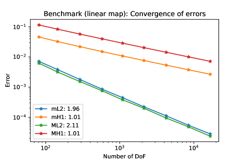
Figure 2: Approximation error as a function of the degrees of freedom. The observed order of convergence is computed from the final step

The convergence of the numerical scheme behaves as expected; The behavior of $e_{uv}$ and $e_{w}$ indicates that the finite element solution converges quadratically to the solution of the PDE. Furthermore, $e_{v}^{\nabla}$ and $e_{uw}^{\nabla}$ indicate that the gradient of the finite element solution converges linearly to the gradient of the solution, also according to expectation.

4.3 Parallel benchmarking

We assess the scalability of the implementation by running it in on a multicore CPU part of the Swedish HPC cluster Kebnekaise. This CPU consists of 28 Intel Xeon nodes with a base frequency of 2.60 GHz. In order to test the parallel scalability of the implementation for different configurations we run two cases: A fine macroscopic grid with coarse microscopic systems and a coarse macroscopic grid with fine microscopic grids. In the first case, the macroscopic system has 4225 degrees of freedom while the microscopic systems each have 81 degrees of freedom. In the second case, the macroscopic system has 81 degrees of freedom while the microscopic systems each have 4225 degrees of freedom.

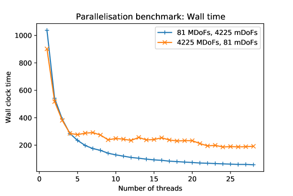
Figure 3: Wall time (total duration of the simulation) as a function of the number of nodes for a fine-macro/coarse-micro system and a coarse-macro/fine-micro system.

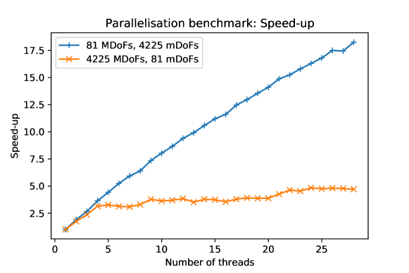
Figure 4: Speed-up as a function of the number of nodes for a fine-macro/coarse-macro system and a coarse-macro/fine-micro system.

Figure 3 displays the duration of the simulation as a function of the number of threads for both configurations. We observe great parallelization performance for runs with fine microscopic grids, but rather poor scalability for runs with fine macroscopic grids. This observation is supported by Figure 4, displaying the speed-up for increasing numbers of nodes. Here it shows that the speed-up of the fine macroscopic grid trails off after 4 threads, while the fine microscopic grids remains scalable at the maximum tested number of 28 threads.

That the parallel performance favors a system with a few fine microscopic grids is a consequence of the implementation. The large microscopic grids mean that there are a lot of individual cells to be assembled, resulting in a lot of independent tasks. This is where a thread-pool performs best.

If one would face the opposite situation; a lot of coarse microscopic grids, one can rely on alternative parallelization strategies. By parallelizing per microscopic system rather than parallelizing per cell, the large number of tasks would once again be independent. The downside of this strategy is that it since the domain deformations are non-linear, it requires duplication of the finite element assembly objects for each microscopic grid, which would place a much larger demand on memory and increases computational load as well.

4.4 Dependence of the microscopic geometry

Having tested and benchmarked the implementation, we use it to solve (5) and examine the dependence of the solution of the microscopic geometry.

We solve (5) using the data presented in Table 3, using the following domain deformation maps.

$$\begin{split}\zeta_{0}(x,y)&:=\begin{pmatrix}y_{1}\\ y_{2}\end{pmatrix},\\ \zeta_{1}(x,y)&:=\frac{1}{20}\begin{pmatrix}-4x_{2}y_{2}+5y_{1}(2x_{1}+3)\\ 5y_{2}(2-x_{2})\end{pmatrix}.\end{split}$$ (20)

We investigate two settings: Case $A$ and Case $B$. As before, $\varOmega=[-1,1]^{2}$, $Z=[-1,1]^{2}$. We model $\partial\varOmega^{\mathrm{D}}=-1\times\left(-1,1\right)$ as a constant source of nutrient $u$. The macroscopic finite element system has 81 degrees of freedom and each microscopic system has 4225 degrees of freedom. In both cases there is no bulk production of any of the species whilst the Dirichlet boundary condition imposed on the left-hand boundary is taken constant. The lack of bulk production terms is enforced to highlight the role played by the microstructure on the macroscopic profiles. In Case $A$ the mapping describing the microstructure is taken to be the identity whilst in Case $B$ a heterogeneous mapping is chosen which results in more elongated cells as the distance from the Dirichlet boundary increases with cell-size increasing from top to bottom. The map in Case $B$ is designed to caricature the heterogeneity observed due to distance from root tips in real plant tissues [29]. In both cases we set $D^{w}\ll D^{v}$ to account for the fact that intracellular transport is much faster than transport within the tissue.

	Case $A$	Case $B$
$D^{w}$	0.1	0.1
$D^{v}$	1	1
$\kappa_{1}$	0.5	0.5
$\kappa_{2}$	1	1
$\kappa_{3}$	0.25	0.25
$\kappa_{4}$	1	1
$f^{u}$	0	0
$f^{w}$	0	0
$u_{0}$	1	1
$\zeta(x,y)$	$\zeta_{0}(x,y)$	$\zeta_{1}(x,y)$

Table 3: Parameter sets used in numerical experiments of (5). Symbol definitions are presented in (20). Solutions to each case are plotted in Figures 10–10.

The solutions to (5) for the cases presented in Table 3 are displayed in Figures 10–10. The effect of the domain deformation is evident. Both on a microscopic level (as displayed in Figure 10) and a macroscopic level (as seen in Figure 10). We observe a quantitative as well as a qualitative effect of the mapping in the macroscopic solutions, specifically the heterogeneous mapping of Case $B$ destroys the symmetry of the problem along the horizontal center line of the (macroscopic) domain and leads to a larger gradient in the concentration of the product of the cells $w$ (compare the scales in Figures 10 and 10). The main driver here is the effect the mapping has on the volume and the aspect ratio of the macroscopic cells. This preliminary numerical investigation therefore suggests that plant cell geometries could act as a significant determinant of tissue level concentration profiles in transport processes in biological tissues.

From a modeling perspective, the coupling of the system comes in play in two places: the right hand side of the macroscopic equations and the boundary terms of the microscopic equations. By tweaking the parameters, the coupling can be made arbitrarily tight. For instance; taking the limit of $D^{w}$ to 0 yields an algebraic relationship between $v$ and $w$. By contrast, choosing $\kappa_{i}\to 0$ for $i=1,...,4$ eliminates the relation between $u,w$ and $v$ and results in a decoupled system.

One of the downsides of this modeling approach is that if the mapping is anisotropic, the resulting degrees of freedom are not equidistributed. This can cause some issues in the accuracy of the microscopic approximations.

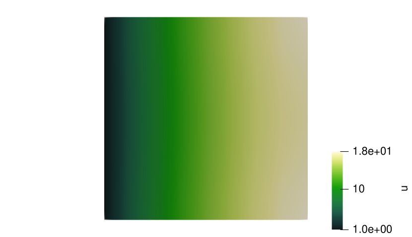
Figure 5: Nutrient concentration $u(x)$ in Case $A$, with the Dirichlet boundary (left) as the only source of nutrient.

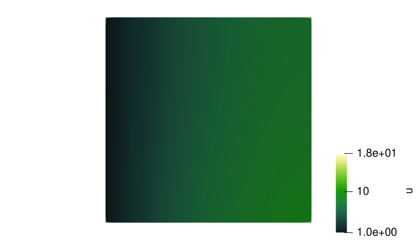
Figure 6: Nutrient concentration $u(x)$ in Case $B$, with the Dirichlet boundary (left) as the only source of nutrient.

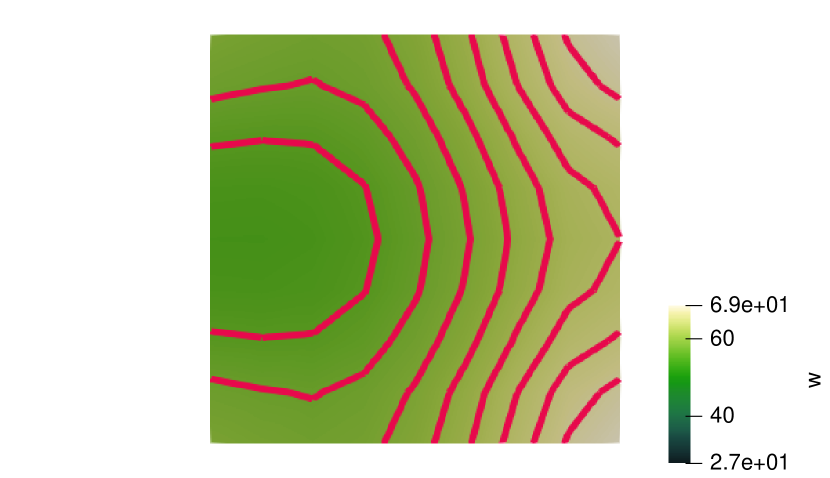
Figure 7: Concentration of the cell product $w(x)$, with the only source of the product the cell-based transmission from $v(x,y)$. Contour indicates level sets.

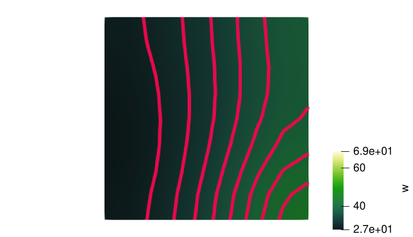
Figure 8: Concentration of the cell product $w(x)$, with the only source of the product the cell-based transmission from $v(x,y)$. Contour indicates level sets.

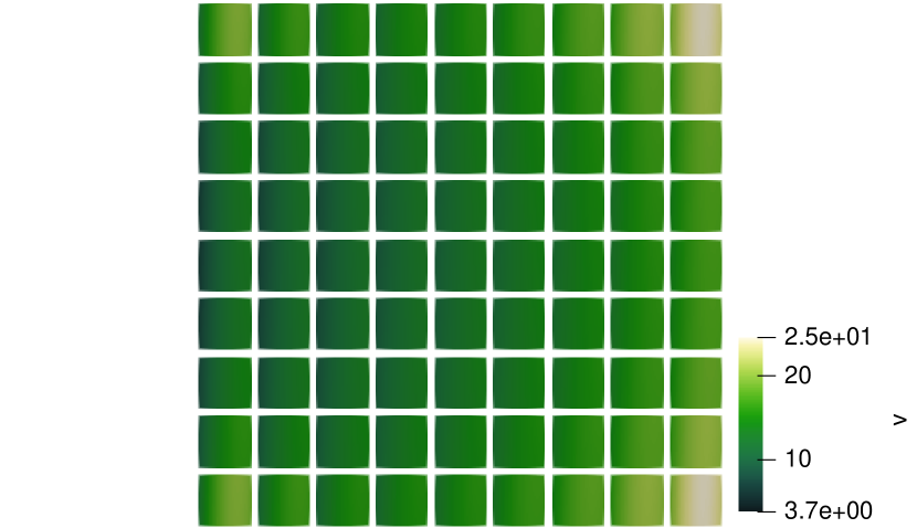
Figure 9: Cell-based nutrient concentration $v(x,y)$ in Case $A$ with an identity domain mapping

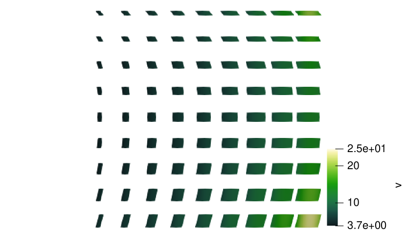
Figure 10: Cell-based nutrient concentration $v(x,y)$, balanced by the consumption of $u(x)$ and the production of $w(x)$.

5 Conclusion

We proposed a parallel finite element treatment of a multiscale model with distributed heterogeneous microstructures. To showcase our framework, we applied it to a system of coupled elliptic PDEs modeling nutrient transport in plants. After imposing a set of constraints on the involved parameters and on the regularity of the macroscopic and microscopic sets so that the underlying coupled system of equations is weakly solvable, we provided a suitable two-scale finite element approximation. Our implementation of this finite element system provides convergent approximations to the weak solution of the original system with the expected theoretical order of convergence. Numerical results demonstrated the influence of the microstructure geometry on both macroscopic and microscopic solution profiles. A parallel implementation scales well for the number of nodes tested.

In practice, the scalability of this setup will not be limited by the implementation; rather, in many cases there might not be access to suitable hardware that has a sufficient number of nodes on a single shared-memory resource. In order to resolve this, we propose the following hybrid parallelization approach: using a macroscopic domain decomposition, we can use classic PDE parallelization techniques to partition the domain on different CPUs, while using the multithreading method to solve each subdomain in parallel on different nodes. This will retain the excellent scaling of the multithreading approach, while also taking full advantage of the performance of parallel domain decomposition. Parallel domain decomposition for single scale problems performs well (see [49, 23, e.g.]) and has been applied in different multiscale finite element contexts as well (see [21, e.g.]). The heterogeneous microstructures are represented and implemented as a continuous map. This allows us to model and compute a family of microscopic domains without explicitly creating meshes for it. The model problem illustrates that, even with relatively simple domain mappings, one retains a lot of modeling flexibility.

Future improvements of this approach should include ways of refining computations at the level of the microscopic systems as a function of error indicators and local geometry. For instance, one improvement to this finite element strategy would be to compute a global microscopic functional: an error indicator defined over all microscopic grids. This quantity could then be used to refine the reference cell and maximize globally the error reduction. Inspired by ideas from [27], another approach would be using random diffeomorphisms instead of deterministic ones. This would allow us to include, under specific conditions, distributions of microscopic defects. It even allows for cases where the choice of the model parameters depends on stationary random ergodic microstructures. We plan to address some of these challenges in a forthcoming work.

References

- [1] A. Abdulle, W. E, B. Engquist, and E. Vanden-Eijnden, The heterogeneous multiscale method, Acta Numerica, 21 (2012), pp. 1–87, https://doi.org/10.1017/S0962492912000025.
- [2] J. Ahrens, B. Geveci, and C. Law, ParaView: An end-user tool for large-data visualization, in The Visualization Handbook, 2005, https://www.researchgate.net/publication/247111133_ParaView_An_End-User_Tool_for_Large_Data_Visualization.
- [3] H. R. Allen and M. Ptashnyk, Mathematical modelling of auxin transport in plant tissues: flux meets signalling and growth, Bulletin of Mathematical Biology, 82 (2020), pp. 1–35, https://doi.org/10.1007/s11538-019-00685-y.
- [4] G. Alzetta, D. Arndt, W. Bangerth, V. Boddu, B. Brands, D. Davydov, R. Gassmoeller, T. Heister, L. Heltai, K. Kormann, M. Kronbichler, M. Maier, J.-P. Pelteret, B. Turcksin, and D. Wells, The deal.II library, version 9.0, Journal of Numerical Mathematics, 26 (2018), pp. 173–183, https://doi.org/10.1515/jnma-2018-0054.
- [5] L. Bin-Ren, Introduction to Operator Algebras, World Scientific, 1992.
- [6] J. Bonet and R. D. Wood, Nonlinear Continuum Mechanics for Finite Element Analysis, Cambridge University Press, 1997.
- [7] A. Chavarría-Krauser and M. Ptashnyk, Homogenization of long-range auxin transport in plant tissues, Nonlinear Analysis: Real World Applications, 11 (2010), pp. 4524–4532, https://doi.org/10.1016/j.nonrwa.2008.12.003.
- [8] W. E, Principles of Multiscale Modeling, Cambridge University Press, 2011.
- [9] Y. Efendiev, J. Galvis, and T. Y. Hou, Generalized multiscale finite element methods (GMsFEM), Journal of Computational Physics, 251 (2013), pp. 116–135, https://doi.org/10.1016/j.jcp.2013.04.045.
- [10] Y. Efendiev and T. Y. Hou, Multiscale Finite Element Methods: Theory and Applications, vol. 4, Springer Science & Business Media, 2009.
- [11] B. Engquist, P. Lötstedt, and O. Runborg, Multiscale Modeling and Simulation in Science, vol. 66, Springer Science & Business Media, 2009.
- [12] L. C. Evans, Partial Differential Equations, vol. 19 of Graduate Studies in Mathematics, American Mathematical Society, Providence, RI, 2010, http://www.worldcat.org/oclc/465190110.
- [13] N. A. Evseev and A. V. Menovschikov, On changing variables in -spaces with distributed-microstructure, Russian Mathematics, 64 (2020), pp. 82–86, https://doi.org/10.3103/S1066369X20030093.
- [14] C. Farhat and F.-X. Roux, A method of finite element tearing and interconnecting and its parallel solution algorithm, International journal for numerical methods in engineering, 32 (1991), pp. 1205–1227, https://doi.org/10.1002/nme.1620320604.
- [15] S. Gärttner, P. Frolkovič, P. Knabner, and N. Ray, Efficiency and accuracy of micro-macro models for mineral dissolution, Water Resources Research, 56 (2020), p. e2020WR027585, https://doi.org/10.1029/2020WR027585.
- [16] C. Godin and Y. Caraglio, A multiscale model of plant topological structures, Journal of Theoretical Biology, 191 (1998), pp. 1–46, https://doi.org/10.1006/jtbi.1997.0561.
- [17] F. Hellman, P. Henning, and A. Målqvist, Multiscale mixed finite elements, Discrete & Continuous Dynamical Systems - S, 9 (2016), https://doi.org/10.3934/dcdss.2016051.
- [18] V. H. Hoang and C. Schwab, High-dimensional finite elements for elliptic problems with multiple scales, Multiscale Modeling & Simulation, 3 (2005), pp. 168–194, https://doi.org/10.1137/030601077.
- [19] U. Hornung and R. E. Showalter, Diffusion models for fractured media, Journal of Mathematical Analysis and Applications, 147 (1990), pp. 69–80, https://doi.org/10.1016/0022-247X(90)90385-S.
- [20] M. F. Horstemeyer, Multiscale modeling: a review, in Practical aspects of computational chemistry, Springer, 2009, pp. 87–135.
- [21] T. Y. Hou and X.-H. Wu, A multiscale finite element method for elliptic problems in composite materials and porous media, Journal of Computational Physics, 134 (1997), pp. 169–189, https://doi.org/10.1006/jcph.1997.5682.
- [22] O. E. Jensen and J. A. Fozard, Multiscale models in the biomechanics of plant growth, Physiology, (2015), https://doi.org/10.1006/jcph.1997.5682.
- [23] A. Klawonn and O. Rheinbach, Highly scalable parallel domain decomposition methods with an application to biomechanics, ZAMM-Journal of Applied Mathematics and Mechanics/Zeitschrift für Angewandte Mathematik und Mechanik: Applied Mathematics and Mechanics, 90 (2010), pp. 5–32, https://doi.org/10.1002/zamm.200900329.
- [24] D. Komatitsch, G. Erlebacher, D. Göddeke, and D. Michéa, High-order finite-element seismic wave propagation modeling with mpi on a large gpu cluster, Journal of computational physics, 229 (2010), pp. 7692–7714, https://doi.org/10.1016/j.jcp.2010.06.024.
- [25] V. Kouznetsova, M. Geers, and W. Brekelmans, Multi-scale second-order computational homogenization of multi-phase materials: a nested finite element solution, Computer Methods in Applied Mechanics and Engineering, 193 (2004), pp. 5525–5550, https://doi.org/10.1016/j.cma.2003.12.073.
- [26] O. Lakkis, A. Madzvamuse, and C. Venkataraman, Implicit–explicit timestepping with finite element approximation of reaction–diffusion systems on evolving domains, SIAM Journal on Numerical Analysis, 51 (2013), pp. 2309–2330, https://doi.org/10.1137/120880112.
- [27] C. Le Bris and F. Legoll, Examples of computational approaches for elliptic, possibly multiscale pdes with random inputs, Journal of Computational Physics, 328 (2017), pp. 455–473, https://doi.org/10.1016/j.jcp.2016.10.027.
- [28] M. Lind, A. Muntean, and O. Richardson, A semidiscrete Galerkin scheme for a coupled two-scale elliptic–parabolic system: well-posedness and convergence approximation rates, BIT Numerical Mathematics, 60 (2020), pp. 999–1031, https://doi.org/10.1007/s10543-020-00805-4.
- [29] J. A. Lockhart, An analysis of irreversible plant cell elongation, Journal of Theoretical Biology, 8 (1965), pp. 264–275, https://doi.org/10.1016/0022-5193(65)90077-9.
- [30] J. Maes and C. Soulaine, A unified single-field volume-of-fluid-based formulation for multi-component interfacial transfer with local volume changes, Journal of Computational Physics, 402 (2020), p. 109024, https://doi.org/10.1016/j.jcp.2019.109024.
- [31] A. Masoudi-Nejad, G. Bidkhori, S. H. Ashtiani, A. Najafi, J. H. Bozorgmehr, and E. Wang, Cancer systems biology and modeling: microscopic scale and multiscale approaches, in Seminars in cancer biology, vol. 30, Elsevier, 2015, pp. 60–69, https://doi.org/10.1016/j.semcancer.2014.03.003.
- [32] S. A. Meier, Two-scale models for reactive transport and evolving microstructure, PhD thesis, Universität Bremen, Germany, 2008.
- [33] S. A. Meier and M. Böhm, A note on the construction of function spaces for distributed-microstructure models with spatially varying cell geometry, Int. J. Numer. Anal. Model, 5 (2008), pp. 109–125.
- [34] A. Meurer, C. P. Smith, M. Paprocki, O. Čertík, S. B. Kirpichev, M. Rocklin, A. Kumar, S. Ivanov, J. K. Moore, S. Singh, T. Rathnayake, S. Vig, B. E. Granger, R. P. Muller, F. Bonazzi, H. Gupta, S. Vats, F. Johansson, F. Pedregosa, M. J. Curry, A. R. Terrel, v. Roučka, A. Saboo, I. Fernando, S. Kulal, R. Cimrman, and A. Scopatz, SymPy: symbolic computing in Python, PeerJ Computer Science, 3 (2017), p. e103, https://doi.org/10.7717/peerj-cs.103.
- [35] A. Muntean and O. Lakkis, Rate of convergence for a Galerkin scheme approximating a two-scale reaction-diffusion system with nonlinear transmission condition, in Nonlinear evolution equations and mathematical modeling, T. Aiki, ed., vol. 1693 of Proceedings RIMS Workshop, Kyoto, Japan, 2010, Research Institute for Mathematical Sciences, RIMS, pp. 85–98, http://arxiv.org/abs/1002.3793. RIMS Workshop held on October 20-23, 2009.
- [36] A. Muntean and M. Neuss-Radu, A multiscale Galerkin approach for a class of nonlinear coupled reaction–diffusion systems in complex media, Journal of Mathematical Analysis and Applications, 371 (2010), pp. 705–718, https://doi.org/10.1016/j.jmaa.2010.05.056.
- [37] G. Pavliotis and A. Stuart, Multiscale Methods: Averaging and Homogenization, Springer Science & Business Media, 2008.
- [38] M. Peszynska and R. E. Showalter, Multiscale elliptic-parabolic systems for flow and transport, Electr. J. Diff. Eqs., 2007 (2007), pp. 1–30.
- [39] P. Raats, Transport in structured porous media, in Proc. Euromech, vol. 143, 1981, pp. 2–4, https://doi.org/10.1023/b:tipm.0000026115.43430.b6.
- [40] P. Raats, Uptake of water from soils by plant roots, Transport in Porous Media, 68 (2007), pp. 5–28, https://doi.org/10.1007/s11242-006-9055-6.
- [41] M. Redeker and C. Eck, A fast and accurate adaptive solution strategy for two-scale models with continuous inter-scale dependencies, Journal of Computational Physics, 240 (2013), pp. 268–283, https://doi.org/10.1016/j.jcp.2012.12.025.
- [42] O. Richardson, Finite element simulation of a two-scale problem implemented in deal.II: 0mar/dealiiscale, 2021, https://github.com/0mar/dealiiscale. original-date: 2019-02-26T11:56:38Z.
- [43] W. Schroeder, K. Martin, and B. Lorensen, VTK Textbook, 2006.
- [44] R. E. Showalter, Distributed microstructure models of porous media, in Flow in Porous Media, U. Hornung, ed., Oberwolfach, 1992, pp. 153–163.
- [45] M. O. Steinhauser, Computational Multiscale Modeling of Fluids and Solids, Springer, 2017.
- [46] J. Twycross, L. R. Band, M. J. Bennett, J. R. King, and N. Krasnogor, Stochastic and deterministic multiscale models for systems biology: an auxin-transport case study, BMC Systems Biology, 4 (2010), pp. 1–11, https://doi.org/10.1186/1752-0509-4-34.
- [47] T. L. van Noorden and A. Muntean, Homogenisation of a locally periodic medium with areas of low and high diffusivity, European Journal of Applied Mathematics, 22 (2011), pp. 493–516, https://doi.org/10.1017/S0956792511000209.
- [48] R. Verfürth, A Posteriori Error Estimation techniques for Finite Element Methods, Numerical Mathematics and Scientific Computation, Oxford University Press, Oxford, 2013, https://doi.org/10.1093/acprof:oso/9780199679423.001.0001, http://www.worldcat.org/oclc/5564393801.
- [49] G. Yagawa and R. Shioya, Parallel finite elements on a massively parallel computer with domain decomposition, Computing Systems in Engineering, 4 (1993), pp. 495–503, https://doi.org/10.1016/0956-0521(93)90017-Q.