Learning Scalable -constrained Near-lossless Image Compression via
Joint Lossy Image and Residual Compression
Abstract
We propose a novel joint lossy image and residual compression framework for learning -constrained near-lossless image compression. Specifically, we obtain a lossy reconstruction of the raw image through lossy image compression and uniformly quantize the corresponding residual to satisfy a given tight error bound. Suppose that the error bound is zero, i.e., lossless image compression, we formulate the joint optimization problem of compressing both the lossy image and the original residual in terms of variational auto-encoders and solve it with end-to-end training. To achieve scalable compression with the error bound larger than zero, we derive the probability model of the quantized residual by quantizing the learned probability model of the original residual, instead of training multiple networks. We further correct the bias of the derived probability model caused by the context mismatch between training and inference. Finally, the quantized residual is encoded according to the bias-corrected probability model and is concatenated with the bitstream of the compressed lossy image. Experimental results demonstrate that our near-lossless codec achieves the state-of-the-art performance for lossless and near-lossless image compression, and achieves competitive PSNR while much smaller error compared with lossy image codecs at high bit rates.
1 Introduction
Image compression is a ubiquitous technique in computer vision. For certain applications with stringent demands on image fidelity, such as medical imaging or image archiving, the most reliable choice is lossless image compression. However, the compression ratio of lossless compression is upper-bounded by Shannon’s source coding theorem [36], and is typically between : and : for practical lossless image codecs [50, 47, 37, 14, 5, 38]. To improve the compression performance while keeping the reliability of the decoded images, -constrained near-lossless image compression is developed [6, 15, 2, 47, 51] and standardized in traditional codecs, \eg, JPEG-LS [47] and CALIC [51]. Different from lossy image compression with Peak Signal-to-Noise Ratio (PSNR) or Multi-Scale Structural SIMilarity index (MS-SSIM) [45, 46] distortion measures, -constrained near-lossless image compression requires the maximum reconstruction error of each pixel to be no larger than a given tight numerical bound. Lossless image compression is a special case of near-lossless image compression, when the tight error bound is zero.
With the fast development of deep neural networks (DNNs), learning-based lossy image compression [40, 3, 39, 41, 34, 24, 4, 31, 27, 22, 8, 7, 23, 25, 29] has achieved tremendous progress over the last four years. Most recent methods for lossy image compression adopt variational auto-encoder (VAE) architecture [17, 18] based on transform coding [11], where the rate is modeled by the entropy of quantized latent variables and the reconstruction distortion is measured by PSNR or MS-SSIM. Through end-to-end rate-distortion optimization, the state-of-the-art methods, such as [7], can achieve comparable performance with the lastest compression standard Versatile Video Coding (VVC) [32]. However, the above transform coding scheme cannot be directly employed on near-lossless image compression, because it is difficult for DNN-based transforms to satisfy a tight bound on the maximum reconstruction error of each pixel, even without quantization. Invertible transforms, such as integer discrete flow [13] or wavelet-like transform [25], are possible solutions to lossless compression but not to general near-lossless compression.
In this paper, we propose a new joint lossy image and residual compression framework for learning near-lossless image compression, inspired by the traditional “lossy plus residual” coding scheme [10, 26, 2]. Specifically, we obtain a lossy reconstruction of the raw image through lossy image compression and uniformly quantize the corresponding residual to satisfy the given error bound . Suppose that the error bound is zero, \ie, lossless image compression, we formulate the joint optimization problem of compressing both the lossy image and the original residual in terms of VAEs [17, 18], and solve it with end-to-end training. Note that our VAE model is novel, different from transform coding based VAEs [3, 39, 4] for simply lossy image compression or bits-back coding based VAEs [42, 19] for lossless image compression.
To achieve scalable near-lossless compression with error bound , we derive the probability model of the quantized residual by quantizing the learned probability model of the original residual at , instead of training multiple networks. Because residual quantization leads to the context mismatch between training and inference, we further propose a bias correction scheme to correct the bias of the derived probability model. An arithmetic coder [48] is adopted to encode the quantized residual according to the bias-corrected probability model. Finally, the near-lossless compressed image is stored including the bitstreams of the encoded lossy image and the quantized residual.
Our main contributions are summarized as follows:
-
•
We propose a joint lossy image and residual compression framework to realize learning-based lossless and near-lossless image compression. The framework is interpreted as a VAE model and can be end-to-end optimized.
-
•
We realize scalable compression by deriving the probability model of the quantized residual from the learned probability model of the original residual, instead of training multiple networks. A bias correction scheme further improves the compression performance.
-
•
Our codec achieves the state-of-the-art performance for lossless and near-lossless image compression, and achieves competitive PSNR while much smaller error compared with lossy image codecs at high bit rates.
2 Related Work
Learning-based Lossy Image Compression. Early learning-based methods [40, 41] for lossy image compression are based on recurrent neural networks (RNNs). Following [3, 39], most recent learned methods [34, 24, 4, 31, 27, 22, 8, 7, 23, 25, 29] adopt convolutional neural networks (CNNs) and can be interpreted as VAEs [17, 18] based on transform coding [11]. In our joint lossy image and residual compression framework, we take advantage of the advanced transform (network structures), quantization and entropy coding techniques in the existing learning-based methods for lossy image compression.
Learning-based Lossless Image Compression. Given the strong connections between lossless compression and unsupervised learning, auto-aggressive models [33, 43, 35], flow models [13], bits-back coding based VAEs [42, 19] and other specific models [28, 30, 25], are introduced to approximate the true distribution of raw images for entropy coding. Previous work [30] uses traditional BPG lossy image codec [5] to compress raw images and proposes a CNN to further compress residuals, which is a special case of our framework. Beyond [30], our lossy image compressor and residual compressor are jointly optimized through end-to-end training and are interpretable as a VAE model.
Near-lossless Image Compression. Basically, previous methods for near-lossless image compression can be divided into three categories: 1) pre-quantization: adjusting raw pixel values to the error bound, and then compressing the pre-processed images with lossless image compression, \eg, near-lossless WebP [14]; 2) predictive coding: predicting subsequent pixels based on previously encoded pixels, then quantizing predication residuals to satisfy the error bound, and finally compressing the quantized residuals, \eg, [6, 15], near-lossless JPEG-LS [47] and near-lossless CALIC [51]; 3) lossy plus residual coding: similar to 2), but replacing predictive coder with lossy image coder, and both the lossy image and the quantized residual are encoded, \eg, in [2].
In this paper, we propose a joint lossy image and residual compression framework for learning-based near-lossless image compression, inspired by lossy plus residual coding. To the best of our knowledge, we propose the first deep-learning-based near-lossless image codec. Recently, CNN-based soft-decoding methods [52, 53] are proposed to improve the reconstruction performance of near-lossless CALIC [51]. However, these methods should belong to image reconstruction rather than image compression.
3 Scalable Near-lossless Image Compression
3.1 Overview of Compression Framework
Given a tight bound , near-lossless codecs compress a raw image satisfying the following distortion measure:
| (1) |
where and are a raw image and its near-lossless reconstructed counterpart. and are the pixels of and , respectively. denotes the -th spatial position in 2D raster-scan order, and denotes the -th channel.
In order to realize the error bound (1), we propose a near-lossless image compression framework by integrating lossy image compression and residual compression. We first obtain a lossy reconstruction of the raw image through lossy image compression. Lossy image compression methods, such as traditional [44, 37, 14, 5] or learned methods [24, 4, 31, 27, 22, 8, 7, 23, 25], can achieve high PSNR results at relatively low bit rates, but it is difficult for these methods to ensure a tight error bound of each pixel in . We then compute the residual and suppose that is quantized to . Let , the reconstruction error is equivalent to the quantization error of . Thus, we adopt a uniform residual quantizer whose bin size is and quantized value is [47, 51]:
| (2) |
where denotes the sign function. and are the elements of and , respectively. With (2), we now have for each in , satisfying the tight error bound (1). Finally, we encode and concatenate it with the compressed , and send them to the decoder.
To compress both the lossy image and the quantized residual effectively leads to a challenging joint optimization problem. In the following subsections, we first propose an end-to-end trainable VAE model [17, 18] to solve the joint optimization problem with . Then, we propose a scalable compression scheme with bias correction for based on the learned VAE model.
3.2 Joint Lossy Image & Residual Compression
Before addressing the joint compression of the lossy image and the quantized residual with variable , we first solve the special case of near-lossless image compression with , \ie, lossless image compression.
Problem Formulation. Assuming that raw images are sampled from an unknown probability distribution , the compression performance of lossless image compression depends on how well we can approximate with an underlying model . We adopt the latent variable model which is formulated by a marginal distribution . is an unobserved latent variable and denote the parameters of this model.
Since directly learning the marginal distribution is typically intractable, one alternative way is to optimize the evidence lower bound (ELBO) via VAEs [17, 18]. By introducing an inference model to approximate the posterior , we can rewrite the logarithm of the marginal likelihood as:
| (3) |
where is the Kullback-Leibler (KL) divergence. denote the parameters of the inference model . Since and , ELBO is the lower bound of .
From (3), we can minimize the expectation of negative ELBO as a proxy for the expected codelength . In our compression framework, we first adopt lossy image compression based on transform coding [11], and the expectation of negative ELBO can be reformulated as follows:
| (4) |
where is quantized from continuous and is transformed from . Like [4], we relax the quantization of by adding noise from , and assume . Thus, is dropped from (4). For simply lossy image compression, such as [4, 31, 8, 7], the first and second terms of (4) are considered as the distortion loss and the rate loss, respectively. Only needs to be encoded.
Beyond lossy image compression, we further take residual compression into consideration. For each and all pairs satisfying , we have . Hence, we substitute for , leading to the upper bound of (4). Let , we have:
| (5) |
The lossy reconstruction is computed by the inverse transform of and quantization. As the quantization is relaxed by adding uniform noise from , we have . The second term and the third term of (5) are the rates of encoding and , respectively.
Notice that no distortion loss of lossy image compression is specified in (5). Therefore, we can embed arbitrary lossy image compressors and optimize (5) to achieve lossless image compression. A special case is the previous lossless image compression method [30], in which the BPG lossy image compressor [5] with a learned quantization parameter classifier optimizes and a CNN-based residual compressor optimizes .
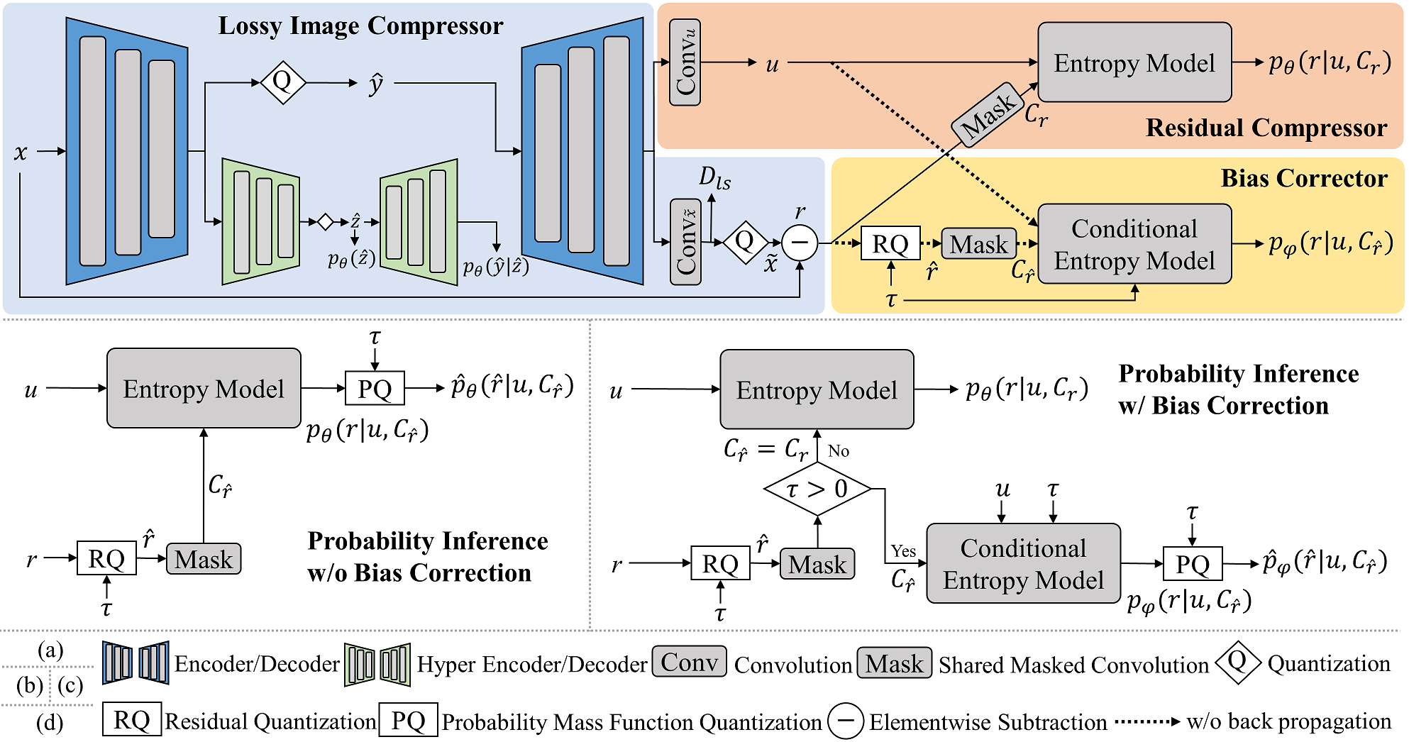
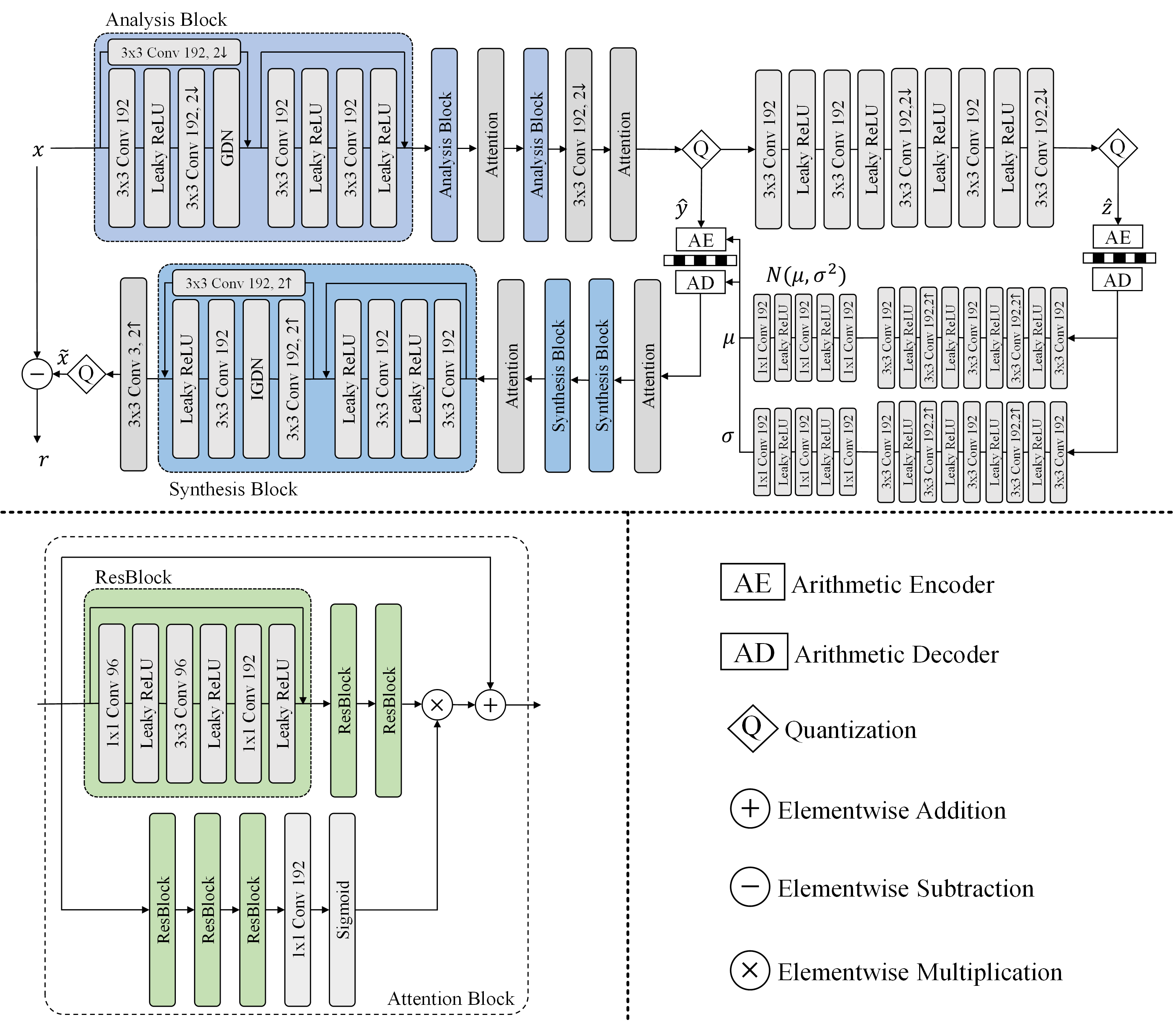
Network Design and Optimization. To realize (5), we propose our network architecture in Fig. 1(a). For lossy image compression, we employ the hyper-prior model proposed in [4], where side information is extracted to model the distribution of . We employ the residual and attention blocks similar to [7, 12] in the encoder and decoder. Detailed structure of the lossy image compressor is described in the supplementary material. is thus extended by
| (6) |
where is the cost of encoding both and .
Denote by , where the feature is extracted from by . Denote by , where the lossy reconstruction is inversely transformed from by . and share the decoder, and only the last convolutional layers are different, as shown in Fig. 1(a). We interpret as the feature of the residual given and ( shares the same height and width with and has 64 channels). As , we can compute and further consider the causal context of during encoding. is thus extended by
| (7) |
where the causal context is shared by of all channels. is extracted from by a masked convolutional layer [31] with 64 channels. denote the residuals encoded before . For RGB images with three channels, we have
| (8) |
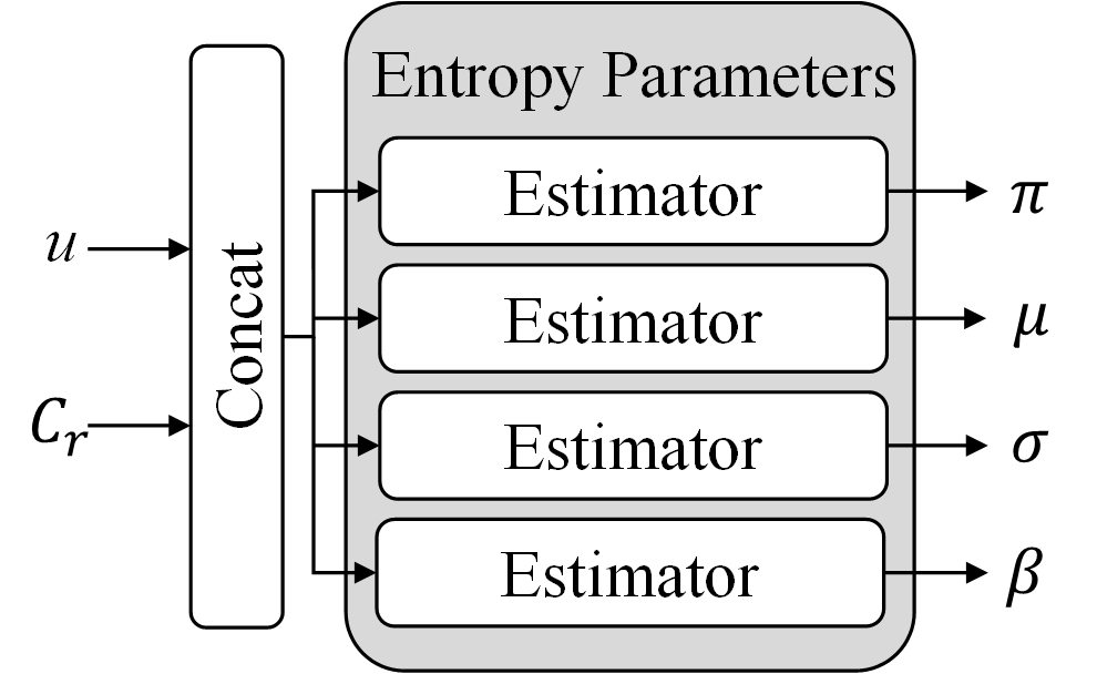
We further model the probability mass function (PMF) of the residual with discrete logistic mixture likelihood [35, 28, 30]. We use a channel autoregression over and reformulate as
| (9) | ||||
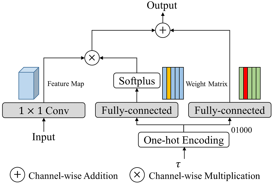
As shown in Fig. 2, we introduce a sub-network to estimate entropy parameters, including mixture weights , means , variances and mixture coefficients . We choose a mixture of logistic distributions. denotes the index of the -th logistic distribution. denotes the channel index of . The channel autoregression over is implemented by updating the means using:
| (10) |
With , and , we have
| (11) |
where is the logistic distribution. For discrete , we evaluate as [35, 28, 30]:
| (12) |
where denotes the sigmoid function. and .
Besides rate terms and , we add a distortion term to minimize the mean square error (MSE) between raw image and lossy reconstruction . As discussed in [4], minimizing MSE loss is equivalent to learning a lossy image compressor that fits residual to a zero-mean factorized Gaussian distribution. However, the discrepancy between the real distribution of and the Gaussian distribution could be large. Thus, a more sophisticated entropy model is proposed to encode . The full loss function for learning near-lossless image compression with , \ie, lossless image compression, is
| (13) |
where controls the “rate-distortion” trade-off. When , becomes a latent variable without any constraints. It leads to the best lossless compression performance but is not suitable for our near-lossless image compression with . We choose empirically in our codec. Experiments with different ’s are conducted in Sec. 4.4.
3.3 Probability Inference of Quantized Residuals
We next propose a scheme to achieve scalable near-lossless image compression with . For variable error bound , we keep the lossy reconstruction fixed and quantize the residual to by (2). Instead of training multiple networks for variably quantized , we derive the probability model of from the learned probability model of at . The resulting cost of encoding , denoted by , is reduced significantly with the increase of .
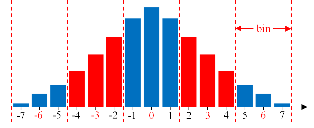
Given and the learned PMF , of quantized can be computed by the following PMF quantization:
| (14) |
An illustrative example is shown in Fig. 3. Together with (8) and (9), we can derive the probability model of , which is ideal given the learned of .
However, encoding with results in undecodable bitstreams, since the original residual is unknown to the decoder. cannot be evaluated without and causal context . Instead, we evaluate PMF using the quantized residual . Because of the mismatch between training (with ) and inference (with ) phases, it leads to a biased PMF of . We then evaluate with (14) and derive for the encoding of . The above probability inference scheme is sketched in Fig. 1(b).
3.4 Bias Correction
Because of the potential discrepancy between the ideal and the biased , encoding with degrades the compression performance. We further propose a bias correction scheme to close the gap between the ideal and the biased , while the resulting bitstreams are still decodable.
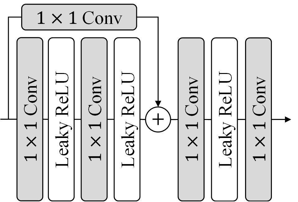
The components of the proposed bias corrector are illustrated in Fig. 1(a). The masked convolutional layer in the bias corrector is shared with that in the residual compressor. The conditional entropy model has the same structure as the entropy model illustrated in Fig. 2, but replaces the convolutional layers with the conditional convolutional layers [43, 8] illustrated in Fig. 4.
During training, we generate random and quantize to with (2). We choose in this paper. Given and the extracted context , we use the conditional entropy model to estimate conditioned on different , and minimize
| (15) |
where denote the parameters of the conditional entropy model. is estimated by the entropy model in the residual compressor. can be considered as an approximate KL-divergence or relative entropy [9] between and . Because the entropy model receives the context extracted from the original residual and is only trained with , approximates the true distribution better than . Thus, is the lower bound of on average.
The probability inference scheme with bias correction is sketched in Fig. 1(c). For , we choose the entropy model to estimate to encode . For , we choose the conditional entropy model to estimate and derive with (14) to encode . As approximates the ideal better than the biased , the compression performance can be improved. Since evaluating is independent of , the resulting bitstreams are decodable. We analyze the efficacy of the proposed bias correction scheme in Sec. 4.4.
Training Strategy. Bias corrector is trained together with the lossy image compressor and the residual compressor, but minimizing (15) only updates the parameters of the conditional entropy model as shown in Fig. 1(a). The masked convolutional layer is shared with that in the residual compressor, thus can be updated by minimizing (13). This leads to three advantages: 1) achieving the target conditional entropy model; 2) circumventing the relaxation of residual quantization; 3) avoiding degrading the estimation of caused by training with mixed .
4 Experiments
4.1 Experimental Setup
Training. We train on DIV2K high resolution training dataset [1] consisting of 800 2K resolution color images. Although DIV2K is originally built for image super-resolution task, it contains large numbers of high-quality images that is suitable for training our near-lossless codec. The images are first cropped into 27958 samples with the size of . To augment training data and prevent overfitting on noise, we use bicubic method to downscale each sample with a random factor selected from and further randomly crop the downscaled sample to during training. Our near-lossless codec is optimized for 400 epochs using Adam [16] with minibatches of size . The learning rate is set to for the first 350 epochs and decays to for the remaining 50 epochs.
Evaluation. We evaluate our near-lossless codec on four datasets: 1) Kodak dataset [20] consists of 24 uncompressed color images. 2) DIV2K high resolution validation dataset [1] consists of 100 2K resolution color images. 3) CLIC professional validation dataset (CLIC.p) [49] consists of 41 color images taken by professional photographers. 4) CLIC mobile validation dataset (CLIC.m) [49] consists of 61 color images taken using mobile phones. Images in CLIC.p and CLIC.m are typically 2K resolution but some of them are of small sizes.
| Codec | Kodak | DIV2K | CLIC.p | CLIC.m |
| PNG | 4.35 | 4.23 | 3.93 | 3.93 |
| JPEG-LS | 3.16 | 2.99 | 2.82 | 2.53 |
| CALIC | 3.18 | 3.07 | 2.87 | 2.59 |
| JPEG2000 | 3.19 | 3.12 | 2.93 | 2.71 |
| WebP | 3.18 | 3.11 | 2.90 | 2.73 |
| BPG | 3.38 | 3.28 | 3.08 | 2.84 |
| FLIF | 2.90 | 2.91 | 2.72 | 2.48 |
| L3C | 3.09 | 2.94 | 2.64 | |
| RC | 3.08 | 2.93 | 2.54 | |
| Ours | 3.04 | 2.81 | 2.66 | 2.51 |
| Codec | Kodak | DIV2K | CLIC.p | CLIC.m | |
| JPEG- LS | 1 | 2.90 | 2.62 | 2.34 | 2.44 |
| 2 | 2.30 | 2.07 | 1.80 | 1.89 | |
| 4 | 1.68 | 1.53 | 1.28 | 1.35 | |
| CALIC | 1 | 2.75 | 2.45 | 2.18 | 2.28 |
| 2 | 2.14 | 1.88 | 1.62 | 1.70 | |
| 4 | 1.51 | 1.31 | 1.07 | 1.13 | |
| WebP nll | 1 | 2.41 | 2.45 | 2.26 | 2.11 |
| 2 | 2.01 | 2.04 | 1.89 | 1.85 | |
| 4 | 1.82 | 1.83 | 1.73 | 1.75 | |
| Ours w/ bc | 1 | 1.84 | 1.72 | 1.60 | 1.53 |
| 2 | 1.38 | 1.29 | 1.15 | 1.10 | |
| 4 | 0.92 | 0.89 | 0.74 | 0.72 |
4.2 Performance Evaluation at
We first evaluate the compression performance of the proposed near-lossless image codec at , measured by bits per subpixel (bpsp). Each RGB pixel has 3 subpixels. We compare with seven traditional lossless image codecs, \ie, PNG, JPEG-LS [47], CALIC [50], JPEG2000 [37], WebP [14], BPG [5], FLIF [38], and two the state-of-the-art learned lossless image codecs, \ie, L3C [28] and RC [30]. Unlike ours, L3C [28] and RC [30] are trained on a much larger dataset (300,000 images from the Open Images dataset [21]). We report the compression performance of L3C [28] and RC [30] published by their authors.
As reported in Table 1, our codec achieves the best performance on DIV2K validation dataset, which shares the same domain with the training dataset. Our codec achieves the best performance on CLIC.p, and the second best performance on Kodak and CLIC.m, only secondary to FLIF. The results demonstrate that the jointly learned lossy image compressor and residual compressor with can effectively model and can be generalized to various domains of natural images. This provides a solid foundation for the near-lossless image compression with .
4.3 Performance Evaluation at
We next evaluate the compression performance of the proposed near-lossless image codec (with bias correction) at . We compare with near-lossless JPEG-LS [47], near-lossless CALIC [51] and near-lossless WebP (WebP nll) [14]. Besides, we compare with six traditional lossy image codecs, \ie, JPEG [44], JPEG2000 [37], WebP [14], BPG [5], lossy FLIF [38] and VVC [32]. Recent learned lossy image codecs published online are trained at relatively low bit rates ( bpp bpsp on Kodak). We re-implement and train two recent learned lossy image codecs, \ie, Ballé-hyper [4] and Minnen-joint [31], at high bit rates ( bpsp on Kodak) for comparison.
Near-lossless WebP simply adjusts pixel values to the error bound and compresses the pre-processed images losslessly. Near-lossless JPEG-LS and CALIC adopt predictive coding schemes, and encode the prediction residuals quantized by (2). The predictors and the probability models used in near-lossless JPEG-LS and CALIC are hand-crafted, which are not effective enough. More effectively, our near-lossless codec is based on jointly trained lossy image compressor and residual compressor. We employ (2) to realize the error bound and the probability models of the quantized residuals can be derived from the learned residual compressor with . Therefore, our codec outperforms near-lossless JPEG-LS, CALIC and WebP by a wide margin, as shown in Table 2.
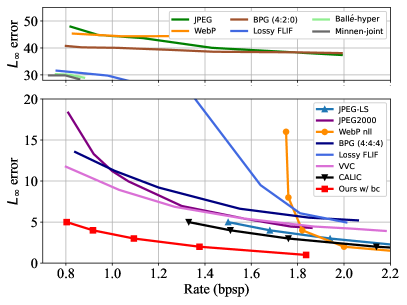
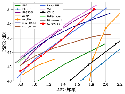
The rate-distortion performance of all codecs on Kodak dataset is reported in Fig. 5. In terms of error defined in (1), our codec consistently yields the best results among all codecs, as shown in Fig. LABEL:sub@fig:rd_error. Besides error, we also compare PSNR of all codecs, as shown in Fig. LABEL:sub@fig:rd_psnr. Our codec is better than or comparable with JPEG, near-lossless JPEG-LS, near-lossless CALIC, WebP, near-lossless WebP, BPG (4:2:0) and lossy FLIF. Our codec is surpassed by JPEG2000, BPG (4:4:4), VVC, Ballé-hyper and Minnen-joint. Overall, our codec achieves competitive performance at bit rates higher than bpsp, although PSNR is not our optimization objective.
4.4 Ablation Study
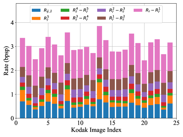
Scalability. In Fig. 6, we show the bit rates of each image compressed by the proposed near-lossless image codec with on Kodak dataset. , on average, accounts for about of at . With the increase of , the bit rate of the quantized residual is significantly reduced. Especially the mode saves about bit rates compared with the lossless image compression mode.

| Total Rate | (PSNR) | |||
| 0 | 2.93 | 0.05 | 2.88 | 24.09 |
| 0.01 | 3.00 | 0.42 | 2.58 | 37.55 |
| 0.03 | 3.04 | 0.55 | 2.49 | 39.29 |
| 0.05 | 3.06 | 0.62 | 2.44 | 39.91 |


Bias Correction. In Fig. 7, we demonstrate the efficacy of bias correction at . Because of the discrepancy between the ideal and the biased , encoding with (without bias correction) degrades the compression performance. Instead, we encode with (with bias correction) resulting in lower bit rates. With the increase of , the PMF of is quantized by larger bins and becomes coarser. Thus, the compression performance with bias correction approaches the “ideal”. However, the gap between the compression performance without bias correction and the “ideal” remains large, as the discrepancy between and is also magnified with the increasing . Note that the compression performance of our codec without bias correction is also better than near-lossless JPEG-LS, CALIC and WebP.
Discussion on different ’s. The in (13) adapts the rate of losslessly encoding the raw image and the distortion of the lossy reconstruction . In Table 3, we evaluate the effects of different on Kodak dataset. With the increase of , the PSNR of is improved but the bpsp of encoding also becomes higher. If we simply do lossless image compression (), we should choose . The is learned by the network without any hand-crafted constraints, leading to the best compression performance.
However, is not suitable for our near-lossless codec with . As the average PSNR of the is dB, the magnitude of is large. To quantize such large residuals with large results in blocking artifacts in the near-lossless reconstruction . As shown in Fig. LABEL:sub@fig:p21_0_ls, with is blurry. If , the quantization bin size is large, \ie, , resulting in blocking artifacts in in Fig. LABEL:sub@fig:p21_0_5. For , we also observe small artifacts in caused by quantization with large , as shown in Fig. LABEL:sub@fig:p09_1_5. In our codec, we choose , which is the best trade-off between compression performance and visual quality in the experiments. As shown in Fig. LABEL:sub@fig:p21_3_5 and Fig. LABEL:sub@fig:p09_3_5, we observe no artifacts in compared with .
5 Conclusion
In this paper, we propose a joint lossy image and residual compression framework to learn a scalable -constrained near-lossless image codec. With our codec, a raw image is first compressed by the lossy image compressor, and the corresponding residual is then quantized to satisfy variable error bounds. To compress the variably quantized residuals, the probability models of the quantized residuals are derived from the learned probability model of the original residual, which is realized by the residual compressor in conjunction with the bias corrector. Experimental results demonstrate the state-of-the-art performance of our near-lossless image codec.
Acknowledgement
This work was supported by National Natural Science Foundation of China under Grants 61922027, 61827804 and U20B2052, National Key Research and Development Project under Grant 2019YFE0109600, China Postdoctoral Science Foundation under Grant 2020M682826.
Appendix A Lossy Image Compressor Architecture
As shown in Fig. 9, we employ the hyper-prior model proposed in [4], where side information is extracted to model the distribution of . We employ the residual and attention blocks to model analysis/synthesis transforms, similar to [7, 12].
Appendix B Proof of Entropy Reduction Resulting from Uniform Quantization
Proposition 1.
Let be a discrete random variable with probability mass function (PMF) , where and are two integers. Suppose that is quantized to by
| (16) |
where denotes the sign function and is an integer. The PMF of the quantized is
| (17) |
Let and be the entropy of and respectively, we have
| (18) |
In words, uniformly quantizing with (16) leads to entropy reduction.
Proof.
Proposition 1 is the theoretical foundation for our scalable compression scheme corresponding to residual quantization.
Appendix C More Visual Results
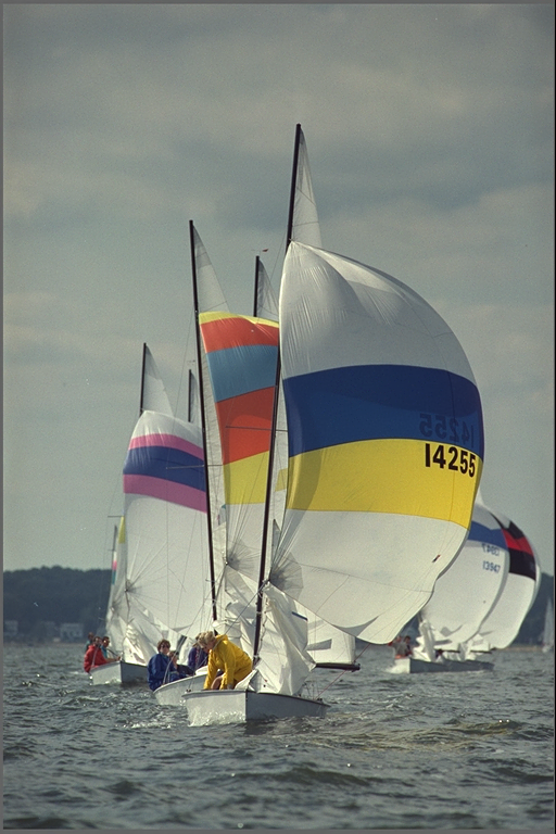
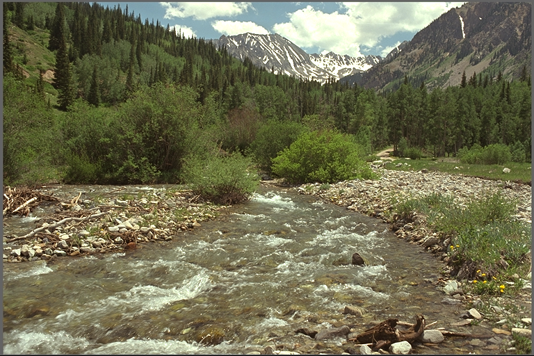
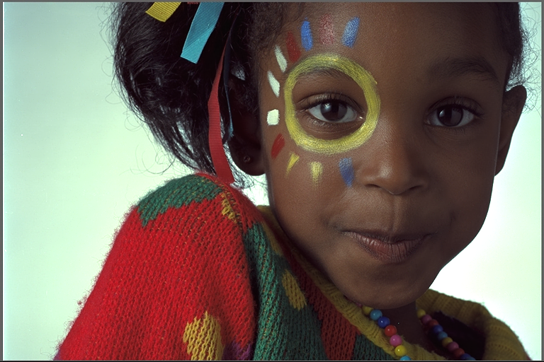
We show more visual results of the near-lossless reconstructions of our codec on Kodak dataset [20] in Fig. 10, 11, 12 and 13. Compared with the raw images, no visual artifacts are introduced by residual quantization. Human eyes can hardly differentiate between the the raw images and the near-lossless reconstructions of our codec at .


References
- [1] Eirikur Agustsson and Radu Timofte. NTIRE 2017 challenge on single image super-resolution: dataset and study. In IEEE Conf. Comput. Vis. Pattern Recog. Worksh., July 2017.
- [2] Rashid Ansari, Nasir D. Memon, and Ersan Ceran. Near-lossless image compression techniques. Journal of Electronic Imaging, 7(3):486 – 494, 1998.
- [3] Johannes Ballé, Valero Laparra, and Eero P Simoncelli. End-to-end optimized image compression. In Int. Conf. Learn. Represent., 2017.
- [4] Johannes Ballé, David Minnen, Saurabh Singh, Sung Jin Hwang, and Nick Johnston. Variational image compression with a scale hyperprior. In Int. Conf. Learn. Represent., 2018.
- [5] Fabrice Bellard. BPG image format. https://bellard.org/bpg/.
- [6] Keshi Chen and Tenkasi V Ramabadran. Near-lossless compression of medical images through entropy-coded dpcm. IEEE Transactions on Medical Imaging, 13(3):538–548, 1994.
- [7] Zhengxue Cheng, Heming Sun, Masaru Takeuchi, and Jiro Katto. Learned image compression with discretized gaussian mixture likelihoods and attention modules. In IEEE Conf. Comput. Vis. Pattern Recog., pages 7939–7948, 2020.
- [8] Yoojin Choi, Mostafa El-Khamy, and Jungwon Lee. Variable rate deep image compression with a conditional autoencoder. In Int. Conf. Comput. Vis., pages 3146–3154, 2019.
- [9] Thomas M. Cover and Joy A. Thomas. Elements of Information Theory (Wiley Series in Telecommunications and Signal Processing). Wiley-Interscience, USA, 2006.
- [10] Sharaf E Elnahas. Data compression with applications to digital radiology. Washington Univ., St. Louis, MO (USA), 1986.
- [11] Vivek K Goyal. Theoretical foundations of transform coding. IEEE Sign. Process. Magazine, 18(5):9–21, 2001.
- [12] Zongyu Guo, Yaojun Wu, Runsen Feng, Zhizheng Zhang, and Zhibo Chen. 3-d context entropy model for improved practical image compression. In IEEE Conf. Comput. Vis. Pattern Recog. Worksh., pages 116–117, 2020.
- [13] Emiel Hoogeboom, Jorn Peters, Rianne van den Berg, and Max Welling. Integer discrete flows and lossless compression. In Adv. Neural Inform. Process. Syst., pages 12134–12144, 2019.
- [14] WebP image format. https://developers.google.com/speed/webp/.
- [15] Ligang Ke and Michael W Marcellin. Near-lossless image compression: minimum-entropy, constrained-error dpcm. IEEE Trans. Image Process., 7(2):225–228, 1998.
- [16] Diederik P Kingma and Jimmy Ba. Adam: A method for stochastic optimization. In Int. Conf. Learn. Represent., 2015.
- [17] Diederik P Kingma and Max Welling. Auto-encoding variational bayes. In Int. Conf. Learn. Represent., 2014.
- [18] Diederik P. Kingma and Max Welling. An introduction to variational autoencoders. Foundations and Trends in Machine Learning, 12(4):307–392, 2019.
- [19] Friso H Kingma, Pieter Abbeel, and Jonathan Ho. Bit-swap: Recursive bits-back coding for lossless compression with hierarchical latent variables. In Int. Conf. Mach. Learn., 2019.
- [20] Eastman Kodak. Kodak lossless true color image suite (photocd pcd0992), 1993. http://r0k.us/graphics/kodak/.
- [21] Ivan Krasin, Tom Duerig, Neil Alldrin, Vittorio Ferrari, Sami Abu-El-Haija, Alina Kuznetsova, Hassan Rom, Jasper Uijlings, Stefan Popov, Andreas Veit, et al. Openimages: A public dataset for large-scale multi-label and multi-class image classification. Dataset available from https://github.com/openimages, 2(3):2–3, 2017.
- [22] Jooyoung Lee, Seunghyun Cho, and Seung-Kwon Beack. Context-adaptive entropy model for end-to-end optimized image compression. In Int. Conf. Learn. Represent., May 2019.
- [23] Mu Li, Wangmeng Zuo, Shuhang Gu, Jane You, and David Zhang. Learning content-weighted deep image compression. IEEE Trans. Pattern Anal. Mach. Intell., 2020.
- [24] M. Li, W. Zuo, S. Gu, D. Zhao, and D. Zhang. Learning convolutional networks for content-weighted image compression. In IEEE Conf. Comput. Vis. Pattern Recog., pages 3214–3223, 2018.
- [25] H. Ma, D. Liu, N. Yan, H. Li, and F. Wu. End-to-end optimized versatile image compression with wavelet-like transform. IEEE Trans. Pattern Anal. Mach. Intell., pages 1–1, 2020.
- [26] Paul W Melnychuck and Majid Rabbani. Survey of lossless image coding techniques. In Digital Image Processing Applications, volume 1075, pages 92–100. International Society for Optics and Photonics, 1989.
- [27] F. Mentzer, E. Agustsson, M. Tschannen, R. Timofte, and L. V. Gool. Conditional probability models for deep image compression. In IEEE Conf. Comput. Vis. Pattern Recog., pages 4394–4402, 2018.
- [28] F. Mentzer, E. Agustsson, M. Tschannen, R. Timofte, and L. Van Gool. Practical full resolution learned lossless image compression. In IEEE Conf. Comput. Vis. Pattern Recog., pages 10621–10630, 2019.
- [29] Fabian Mentzer, George Toderici, Michael Tschannen, and Eirikur Agustsson. High-fidelity generative image compression. In Adv. Neural Inform. Process. Syst., 2020.
- [30] Fabian Mentzer, Luc Van Gool, and Michael Tschannen. Learning better lossless compression using lossy compression. In IEEE Conf. Comput. Vis. Pattern Recog., 2020.
- [31] David Minnen, Johannes Ballé, and George D Toderici. Joint autoregressive and hierarchical priors for learned image compression. In Adv. Neural Inform. Process. Syst., pages 10771–10780, 2018.
- [32] Jens-Rainer Ohm and Gary J Sullivan. Versatile video coding–towards the next generation of video compression. In Picture Coding Symposium, 2018.
- [33] Aäron van den Oord, Nal Kalchbrenner, and Koray Kavukcuoglu. Pixel recurrent neural networks. In Int. Conf. Mach. Learn., pages 1747–1756. JMLR.org, 2016.
- [34] Oren Rippel and Lubomir Bourdev. Real-time adaptive image compression. In Int. Conf. Mach. Learn., volume 70, pages 2922–2930, 2017.
- [35] Tim Salimans, Andrej Karpathy, Xi Chen, and Diederik P Kingma. Pixelcnn++: Improving the pixelcnn with discretized logistic mixture likelihood and other modifications. In Int. Conf. Learn. Represent., 2017.
- [36] Claude E Shannon. A mathematical theory of communication. The Bell system technical journal, 27(3):379–423, 1948.
- [37] Athanassios Skodras, Charilaos Christopoulos, and Touradj Ebrahimi. The jpeg 2000 still image compression standard. IEEE Sign. Process. Magazine, 18(5):36–58, 2001.
- [38] Jon Sneyers and Pieter Wuille. Flif: Free lossless image format based on maniac compression. In IEEE Int. Conf. Image Process., pages 66–70. IEEE, 2016.
- [39] Lucas Theis, Wenzhe Shi, Andrew Cunningham, and Ferenc Huszár. Lossy image compression with compressive autoencoders. In Int. Conf. Learn. Represent., 2017.
- [40] George Toderici, Sean M. O’Malley, Sung Jin Hwang, Damien Vincent, David Minnen, Shumeet Baluja, Michele Covell, and Rahul Sukthankar. Variable rate image compression with recurrent neural networks. In Int. Conf. Learn. Represent., 2016.
- [41] George Toderici, Damien Vincent, Nick Johnston, Sung Jin Hwang, David Minnen, Joel Shor, and Michele Covell. Full resolution image compression with recurrent neural networks. In IEEE Conf. Comput. Vis. Pattern Recog., pages 5306–5314, 2017.
- [42] James Townsend, Tom Bird, and David Barber. Practical lossless compression with latent variables using bits back coding. In Int. Conf. Learn. Represent., 2019.
- [43] Aäron van den Oord, Nal Kalchbrenner, Lasse Espeholt, Oriol Vinyals, and Alex Graves. Conditional image generation with pixelcnn decoders. In Adv. Neural Inform. Process. Syst., pages 4790–4798, 2016.
- [44] Gregory K Wallace. The jpeg still picture compression standard. IEEE Trans. Consumer Electronics, 38(1):xviii–xxxiv, 1992.
- [45] Zhou Wang, Alan C Bovik, Hamid R Sheikh, and Eero P Simoncelli. Image quality assessment: from error visibility to structural similarity. IEEE Trans. Image Process., 13(4):600–612, 2004.
- [46] Zhou Wang, Eero P Simoncelli, and Alan C Bovik. Multiscale structural similarity for image quality assessment. In The Thrity-Seventh Asilomar Conference on Signals, Systems & Computers, 2003, volume 2, pages 1398–1402. Ieee, 2003.
- [47] Marcelo J Weinberger, Gadiel Seroussi, and Guillermo Sapiro. The loco-i lossless image compression algorithm: Principles and standardization into jpeg-ls. IEEE Trans. Image Process., 9(8):1309–1324, 2000.
- [48] Ian H Witten, Radford M Neal, and John G Cleary. Arithmetic coding for data compression. Communications of the ACM, 30(6):520–540, 1987.
- [49] Workshop and Challenge on Learned Image Compression. https://www.compression.cc/challenge/.
- [50] X. Wu and N. Memon. Context-based, adaptive, lossless image coding. IEEE Trans. Communications, 45(4):437–444, 1997.
- [51] Wu Xiaolin and P. Bao. constrained high-fidelity image compression via adaptive context modeling. IEEE Trans. Image Process., 9(4):536–542, 2000.
- [52] X. Zhang and X. Wu. Near-lossless -constrained image decompression via deep neural network. In Data Compression Conference, pages 33–42, 2019.
- [53] X. Zhang and X. Wu. Ultra high fidelity deep image decompression with -constrained compression. IEEE Trans. Image Process., 30:963–975, 2021.