Mid-infrared circumstellar emission of the long-period Cepheid $\ell$ Carinae resolved with VLTI/MATISSE

Abstract

Context. The nature of circumstellar envelopes (CSE) around Cepheids is still a matter of debate. The physical origin of their infrared (IR) excess could be either a shell of ionized gas, or a dust envelope, or both.

Aims. This study aims at constraining the geometry and the IR excess of the environment of the bright long-period Cepheid $\ell$ Car (P=35.5 days) at mid-IR wavelengths to understand its physical nature.

Methods. We first use photometric observations in various bands (from the visible domain to the infrared) and Spitzer Space Telescope spectroscopy to constrain the IR excess of $\ell$ Car. Then, we analyze the VLTI/MATISSE measurements at a specific phase of observation, in order to determine the flux contribution, the size and shape of the environment of the star in the $L$ band. We finally test the hypothesis of a shell of ionized gas in order to model the IR excess.

Results. We report the first detection in the $L$ band of a centro-symmetric extended emission around $\ell$ Car, of about $1.7\,R_{\star}$ in full width at half maximum, producing an excess of about $7.0\%$ in this band. This latter value is used to calibrate the IR excess found when comparing the photometric observations in various bands and quasi-static atmosphere models. In the $N$ band, there is no clear evidence for dust emission from VLTI/MATISSE correlated flux and Spitzer data. On the other side, the modeled shell of ionized gas implies a more compact CSE ($1.13\pm 0.02\,R_{\star}$) and fainter (IR excess of 1% in the $L$ band).

Conclusions. We provide new evidences for a compact CSE of $\ell$ Car and we demonstrate the capabilities of VLTI/MATISSE for determining common properties of CSEs. While the compact CSE of $\ell$ Car is probably of gaseous nature, the tested model of a shell of ionized gas is not able to simultaneously reproduce the IR excess and the interferometric observations. Further Galactic Cepheids observations with VLTI/MATISSE are necessary for determining the properties of CSEs, which may also depend on both the pulsation period and the evolutionary state of the stars.

1 Introduction

Circumstellar envelopes (CSEs) around Cepheids have been spatially resolved by long-baseline interferometry in the $K$ band with the Very Large Telescope Interferometer (VLTI) and the Center for High Angular Resolution Astronomy (CHARA) (Kervella et al. 2006; Mérand et al. 2006). They were detected around four Cepheids including $\ell$ Car, in the $N$ band with VLTI/VISIR and VLTI/MIDI (Kervella et al. 2009; Gallenne et al. 2013). In the $K$ band, the diameter of the envelope appears to be at least 2 stellar radii and the flux contribution is up to 5% of the continuum (Mérand et al. 2007). Both the size and flux contribution are expected to be larger in the $N$ band, as demonstrated by Kervella et al. (2009) for $\ell$ Car, Gallenne et al. (2013) for X Sgr and T Mon, and by Gallenne et al. (2021, submitted) for other Cepheids. Moreover, a CSE has also been discovered in the visible domain with the CHARA/VEGA instrument around $\delta$ Cep (Nardetto et al. 2016). The systematic presence of a CSE is still a matter of debate. While some studies have found no significant observational evidence for circumstellar dust envelopes in a large number of Cepheids (Schmidt 2015; Groenewegen 2020), Gallenne et al. (2021, submitted) found a significant IR excess attributed to a CSE for 10 out of 45 Cepheids.
Recently, Hocdé et al. (2020b) (hereafter Paper I) used an analytical model of free-free and bound-free emission from a thin shell of ionized gas to explain the near and mid-IR excess of Cepheids. They found a typical radius for this shell of ionized gas of about $R_{\mathrm{shell}}$=1.15$\,R_{\star}$. This shell of ionized gas could be due to periodic shocks occurring in both the atmosphere and the chromosphere, which heat up and ionize the gas. Using VLT/UVES data, (Hocdé et al. 2020a) found a radius for the chromosphere of at least $R_{\mathrm{chromo}}$=1.5$\,R_{\star}$ in long-period Cepheids. In addition, they found a motionless H$\alpha$ feature in UVES high-resolution spectra obtained for several long-period Cepheids, including $\ell$ Car. This absorption feature was attributed to a static CSE surrounding the chromosphere above at least 1.5$\,R_{\star}$, and reported by various authors around $\ell$ Car (Rodgers & Bell 1968; Bohm-Vitense & Love 1994; Nardetto et al. 2008).
Determining the IR excess and the size of the CSE is a key to understand the physical processes at play. In this paper, we study the long-period Cepheid $\ell$ Car. Our aim is to determine its IR excess from photometric measurements in various bands and Spitzer spectroscopy, while inferring the size of the CSE and its flux contribution thanks to the unique capabilities provided by the Multi AperTure mid-Infrared SpectroScopic Experiment (VLTI/MATISSE; Lopez et al. (2014); Allouche et al. (2016); Robbe-Dubois et al. (2018)) in the $L$ (2.8-4.0$\,\mu$m), $M$ (4.5 - 5$\,\mu$m) and $N$ bands (8 - 13$\,\mu$m).
We first reconstruct the IR excess in Sect 2. Then, we present the data reduction and calibration process of VLTI/MATISSE data in Sect. 3. We use a simple model of the CSE to reproduce the visibility measurement of VLTI/MATISSE in Sect. 4. In Sect. 5 we discuss the physical origin of this envelope, and present a model of a shell of ionized gas. We summarize our conclusions in Sect. 6.

2 Deriving the infrared excess of $\ell$ Car

2.1 Near-IR excess modeling with SPIPS

Due to their intrisic variability, the photospheres of the Cepheids are difficult to model along the pulsation cycle. However, it is an essential prerequisite for deriving both the IR excess in a given photometric band, and the expected angular stellar diameter at a specific phase of interferometric observations (required in Sect. 3). In order to model the photosphere we use SpectroPhoto-Interferometric modeling of Pulsating Stars (SPIPS), which is a model-based parallax-of-pulsation code which includes photometric, interferometric, effective temperature and radial velocity measurements in a robust model fitting process (Mérand et al. 2015).

SPIPS uses a grid of ATLAS9 atmospheric models (Castelli & Kurucz 2003) with solar metallicity and a standard turbulent velocity of 2 km/s. SPIPS was already extensively described and used in several studies (Mérand et al. 2015; Breitfelder et al. 2016; Kervella et al. 2017; Gallenne et al. 2017), Javanmardi et al. (2021, accepted), Gallenne et al. (2021, submitted), and Paper I. SPIPS also takes into account the possible presence of an IR excess by fitting an ad-hoc analytic power law $\mathrm{IR}_{\mathrm{ex}}$ (see green curve in Fig. 1(a)). We note that Gallenne et al. (2021, submitted) have shown that $\ell$ Car possibly has an IR excess using SPIPS, but its low detection level (2.9 ± 3.2% in $K$ band) is not significant compared to a single-star model (i.e. without IR excess model). Breitfelder et al. (2016) also provided a SPIPS fitting of $\ell$ Car which did not present any significant IR excess. However, this work was done by considering only the $V$, $J$, $H$ and $K$ photometric bands, i.e. not the mid-infrared bands, which are critical to detect such an IR excess. Finally, since a CSE around $\ell$ Car has been detected by interferometry in the infrared (Kervella et al. 2006, 2009), we enable SPIPS to fit an IR excess in the following analysis. SPIPS provides a fit to the photometry along the pulsation cycle, which is in agreement with the observational data (description in Appendix 7). From Fig. 7, we emphasize that the SPIPS fitted model is well constrained by the numerous observations, and thus the physical parameters of the photosphere are accurately derived. However, as noted in the SPIPS original paper, the uncertainties on the derived parameters are purely statistical and do not take into account systematics. While the fitting is satisfactory from the visible domain to the near infrared, SPIPS fits an IR excess for wavelengths above about 1.2$\,\mu$m. Indeed the observed brightness ($m_{\mathrm{obs}}$) significantly exceeds the predictions ($m_{\mathrm{kurucz}}$). The averaged IR excess over a pulsation cycle is presented in Fig. 1(a). In the next section we combine this average IR excess with Spitzer mid-infrared spectroscopy.

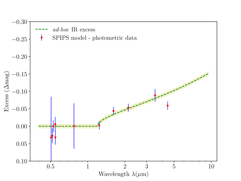
(a) SPIPS cycle-averaged IR excess

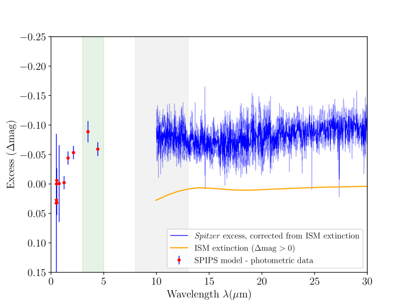
(b) Reconstructed IR excess with SPIPS and Spitzer

Figure 1: (a) Averaged IR excess of $\ell$ Car as derived with the SPIPS algorithm (red dots) and presented with the fitted ad-hoc analytic law $\mathrm{IR}_{\mathrm{ex}}=-0.053(\lambda-1.2)^{0.501}\mathrm{mag}$. For each photometric band (described in Appendix A), the red dots are the mean excess value averaged over the cycle of pulsation of $\ell$ Car while the blue uncertainties correspond to the respective standard deviation. (b) The IR excess of $\ell$ Car is reconstructed at the specific phase of Spitzer observation. It includes the averaged IR excess from SPIPS (red dots) and the Spitzer observations (blue line) corrected for the silicate absorption of the ISM along the line of sight (orange curve). The silicate extinction has been derived using silicate refractive index from Draine & Lee (1984). Green and gray vertical stripes represent the $LM$ and $N$ bands of MATISSE, respectively.

2.2 Mid-IR excess from Spitzer observations

Space-based observations such as those of obtained with the Spitzer space telescope are useful to avoid perturbation caused by the Earth atmosphere, which is essential for the study of dust spectral features. We use spectroscopic observations made with the InfraRed Spectrograph IRS (Houck et al. 2004) on board the Spitzer telescope (Werner et al. 2004). High spectral resolution (R=600) from 10$\,\mu$m to 38$\,\mu$m was used with Short-High (SH) and Long-High (LH) modules placed in the focal plane instrument. The full spectra were retrieved from the CASSIS atlas (Lebouteiller et al. 2011) and the best flux calibrated spectrum was obtained from the optimal extraction using differential method, which eliminates low-level rogue pixels (Lebouteiller et al. 2015). Table 1 provides an overview of the Spitzer observation. The reference epoch at maximum light (MJD₀=50583.742), pulsation period ($P$=35.557 days) and the rate of period change ($\dot{P}$=33.4$\pm 1.0\,$s/yr) used to derive the pulsation phase corresponding to the Spitzer observation are those computed by the SPIPS fitting of $\ell$ Car. We note that the most up-to-date and independent value of rate of period change, derived by Neilson et al. (2016) ($\dot{P}=20.23\pm 1.38\,$s/y) is slightly lower than the value estimated by SPIPS. However adopting this latter value would not change the result of this paper.

Table 1: Spitzer data set of $\ell$ Car (program number 40968). The Astronomical Observation Request (AOR), the date of observation, the corresponding Modified Julian Date (MJD), and the pulsation phase ($\phi$) are indicated. The physical parameters of $\ell$ Car derived by SPIPS at the Spitzer observation phase are indicated: the effective temperature ($T_{\mathrm{eff}}$), the surface gravity (log $g$) and the limb-darkened angular diameter ($\theta_{\mathrm{LD}}$). Statistical uncertainties on $T_{\mathrm{eff}}$ and $\theta$ are provided by SPIPS, whereas uncertainty on log $g$ is arbitrarily set to 10%.

Object	AOR	Date	MJD	$\phi_{\textit{Spitzer}}$	$T_{\mathrm{eff}}(\phi_{\textit{Spitzer}})$	log $g(\phi_{\textit{Spitzer}})$	$\theta_{\mathrm{LD}}(\phi_{\textit{Spitzer}})$
		(yyyy.mm.dd)	(days)		(K)	(cgs)	(mas)
$\ell$ Car	23403520	2008.05.03	54589.502	0.648	$4630^{+15}_{-15}$	$0.98^{+0.10}_{-0.10}$	$2.897^{+0.002}_{-0.002}$

In order to derive the IR excess of Spitzer observation, and correct for the absorption of the interstellar matter (ISM), we followed the method developed in Paper I. First, we derived the IR excess of $\ell$ Car at the specific Spitzer epoch using

$$\Delta\mathrm{mag}=m_{\textit{Spitzer}}-m_{\mathrm{kurucz}}[\phi_{\textit{Spitzer}}]$$ (1)

where $m_{\textit{Spitzer}}$ is the magnitude of the Spitzer observation and $m_{\mathrm{kurucz}}[\phi_{\textit{Spitzer}}]$ is the magnitude of the ATLAS9 atmospheric model interpolated at the phase of Spitzer observations ($\phi_{\textit{Spitzer}}$) using the parameters derived by SPIPS and given in Table 1. We discarded wavelengths of Spitzer observations longer than 30$\,\mu$m due to extremely large uncertainties. Secondly, we corrected the spectrum for ISM extinction by subtracting a synthetic ISM composed of silicates from Draine & Lee (1984) (see orange curve in Fig. 1(b)). This calculation assumes a relation between the extinction E($B-V$) derived by SPIPS (i.e. E($B-V$)=0.148 mag) and the silicate absorption from diffuse interstellar medium (see Eq. 4 in Paper I). Finally, we combine this result with SPIPS averaged IR excess in order to reconstruct the IR excess from the visible to the mid-infrared domain. The determined IR excess is presented in Fig. 1(b) (red dots and blue line).
Similarly to the five Cepheids presented in Paper I, we observe a continuum IR excess increasing up to $-$0.1 mag at 10$\,\mu$m. In particular within the specific bands of MATISSE (see vertical strips in Fig. 1(b)), the IR excess is between $-$0.05 and $-$0.1 mag at 3.5$\,\mu$m and 4.5$\,\mu$m ($L$ and $M$ bands) which represents an excess of 5 to 10% above the stellar continuum. In addition, we find no silicate emission feature in the Spitzer spectrum around 10$\,\mu$m ($N$ band) within the uncertainties, which points toward an absence of significant amount of circumstellar dust with amorphous silicate components.

3 VLTI/MATISSE interferometric observations

MATISSE is the four-telescope beam combiner in the $L$, $M$ and $N$ bands of the Very Large Telescope Interferometer (VLTI). The VLTI array consists of four 1.8-meter auxiliary telescopes (ATs) and four 8-meter unit telescopes (UTs), and provides baseline lengths from 11 meters to 150 meters. As a spectro-interferometer, MATISSE provides dispersed fringes and photometries. The standard observing mode of MATISSE (so-called hybrid) uses the two following photometric measurement modes: SIPHOT for $L$ and $M$ bands, in which the photometry is measured simultaneously with the dispersed interference fringes, and HIGH SENS for $N$ band, in which the photometric flux is measured separately after the interferometric observations. The observations were carried out during the nights of 27 and 28 February 2020 with the so-called large configuration of the ATs quadruplet (A0-G1-J2-J3, with ground baseline lengths from 58 to 132 m) in low spectral resolution (R=$\lambda/\Delta\lambda\approx$30). The log of the MATISSE observations is given in Table 2. The raw data were processed using the version (1.5.5) of the MATISSE data reduction software . The steps of the data reduction process are described in Millour et al. (2016).

The MATISSE absolute visibilities are estimated by dividing the measured correlated flux by the photometric flux. Thermal background effects affect the measurement in the $M$ and $N$ bands significantly more than in the $L$ band. Thus, we use only the $L$ band visibilities in our modeling and analysis, while the $L$ and $M$ photometries are used for deriving the observed total flux (see Sect. 3.2). In the $N$ band, the total flux of $\ell$ Car ($\approx$17 Jy) is at the lower limit of the ATs sensitivity with MATISSE for accurate visibility measurements ($\sim$ 20 Jy, as stated on the ESO webpage of the MATISSE instrument). Thus, we rather use the correlated flux measurements (not normalized by the photometric flux) as an estimate of the $N$ band photometry of $\ell$ Car. In the following of the paper, we discarded the 4.1 to 4.5$\,\mu$m spectral region, where the atmosphere is not transmissive, and also the noisy edges of the atmosphere spectral bands. As a result, we analyze the following spectral region in $L$ (3.1-3.75$\mu$m) for absolute visibility and flux, $M$ (4.75-4.9$\mu$m) for flux, and in $N$ (8.2-12$\mu$m) for correlated flux.

3.1 Calibration of the squared visibility in the $L$ band

Calibrators were selected using the SearchCal tool of the JMMC, with a high confidence level on the derived angular diameter ($\chi^{2}\leq 5$, see Appendix A.2 in Chelli et al. (2016)). Moreover, calibrator fluxes in the $L$ and $N$ bands have to be of the same order than for the science target (i.e. $\approx$10 to 100 Jy in $L$ and $N$) to ensure a reliable calibration (Cruzalèbes et al. 2019). These flux requirements induce the use of partially resolved calibrators at the 132-m longest baseline. The $L$ band uniform-disk (UD) angular diameters for the standard stars as well as the corresponding $L$ and $N$ band fluxes and the spectral type are given in Table 3.
We analyze these calibration stars with a special care. The first calibrator of this night, q Car, was observed in the frame of a different program and was not used in the interferometric visibility calibration process. Indeed, it is a supergiant star of spectral type KII, which makes its angular diameter of 5.2 mas too large (compared to $\ell$ Car), and rather uncertain in the $L$ band. However, q Car appears to be a suitable total flux calibrator for $\ell$ Car in both $L$ and $M$ bands (see Sect. 3.2). Indeed, although q Car is an irregular long-period variable, its photometric variation in the visible is $\Delta$mag$\approx$0.1 (GCVS, Samus’ et al. 2017), thus its flux variation in the Rayleigh-Jeans domain, i.e. in the $L$ and $M$ bands, only represents about 1%. Moreover q Car was observed at an air mass very close to the one of $\ell$ Car (see Table 2). In the analysis, we discarded the calibrator B Cen since it has inconsistent visibilities as explained in Appendix B. Thus, we used $\epsilon$ Ant to calibrate observation $\#$1. For observation $\#$2, we also used $\epsilon$ Ant. For observation $\#3$, we bracketed the science target with the standard CAL-SCI-CAL strategy calibration using $\beta$ Vol. The calibrated squared visibilities ($V^{2}$) in $L$ band are presented in Fig. 2. The visibility curve associated with the limb-darkened angular diameter of the star (without CSE), which was derived from the SPIPS analysis at the specific phase of VLTI/MATISSE ($\phi$=0.07), is shown for comparison.

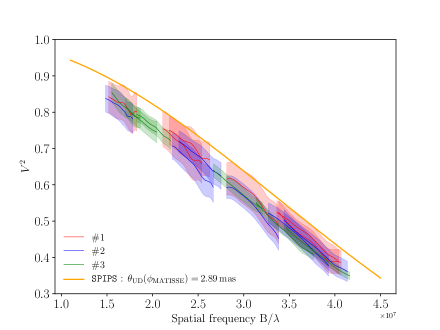
Figure 2: The calibrated squared visibilities of $\ell$ Car as a function of the spatial frequencies in the $L$ band for observations $\#1$, 2 and 3. The theoretical visibility curve corresponding to a uniform disk of $\theta_{\mathrm{UD}}=2.887\pm 0.003\,$mas in the $L$ band, as derived from the SPIPS analysis (i.e. without CSE) is indicated for comparison.

Table 2: Log of the observations for nights of 27 February (observations $\#$1 and 2) and 28 February 2020 (observation $\#$3) with the Modified Julian Date (MJD), the pulsation phase $\phi$, the seeing (in arcsecond), the air mass (AM), integrated water vapour (IWV) at 30 deg elevation (in millimeter) and the coherence time $\tau_{0}$ (in millisecond) are indicated. Stars used in the visibility calibration strategy are marked with an asterisk (see Sect. 3.1). q Car and $\beta$ Vol are used to calibrate the total flux (see Sect. 3.2), while e Cen is used to check the consistency of the other calibrators (see Appendix B). The calibrator B Cen is not used, see Appendix B

.

#	Target	Date	$\phi$	seeing	AM	$\tau_{0}$
		(MJD)		(′′)		(ms)
	q Car	58907.11		0.78	1.40	6.0
1	$\ell$ Car*	58907.12	0.05	0.66	1.32	5.3
	B Cen	58907.13		0.85	1.39	6.1
2	$\ell$ Car*	58907.14	0.05	1.15	1.27	6.0
	$\epsilon$ Ant*	58907.15		0.69	1.02	6.9
	e Cen	58907.28		1.26	1.10	4.8
	bet Vol*	58907.99		0.79	1.51	6.3
3	$\ell$ Car*	58908.00	0.07	0.81	1.66	6.3
	bet Vol*	58908.01		0.91	1.42	15.7

Table 3: Calibrator properties. $\theta_{\mathrm{UD}}$ is the uniform disk (UD) angular diameter in $L$ band from the JSDC V2 catalogue (Bourgés et al. 2014), $F_{L}$ and $F_{N}$ are the flux in the $L$ and $N$ bands from the Mid-infrared stellar Diameters and Fluxes compilation Catalogue (MDFC) (Cruzalèbes et al. 2019).

Calibrator	$\theta_{\mathrm{UD}}$(mas)	$F_{L}$ (Jy)	$F_{N}$(Jy)	Sp. Type
q Car	5.19$\pm$0.60	299.5$\pm$50.6	45.8$\pm 8.2$	K2.5 II
B Cen	2.54$\pm$0.28	72.3$\pm 11.8$	10.6$\pm 1.0$	K3 III
$\epsilon$ Ant	2.86$\pm$0.30	88.1$\pm 1.2$	12.2$\pm 1.8$	K3 III
e Cen	2.97$\pm$0.29	88.9$\pm 10.9$	13.2$\pm 1.6$	K3.5 III
bet Vol	2.90$\pm$0.29	95.4$\pm 23.5$	14.6$\pm 3.4$	K2 III

MATISSE also provides closure phase measurements, which contain information about the spatial centro-symmetry of the brightness distribution of the source. For all the closure phase measurements, we find an average closure phase of about 0^∘ in the $L$, $M$ and the $N$ band from 8.2 to 9.25$\,\mu$m (see Fig. 3). In the $N$ band we indicated the typical peak-to-valley dispersion of the MATISSE closure phase measurements with an error bar ($\approx$10 degrees) and we discarded the spectral region beyond 10$\,\mu$m due to extremely large uncertainties (see Fig. 3). Down to a sub-degree level (resp. 10 degrees level), our closure phase measurements are consistent with the absence of significant brightness spatial asymmetries in the environment around $\ell\leavevmode\nobreak\$Car in $L$ and $M$ bands (resp. $N$ band). That justifies our use of centro-symmetric models in the following of the paper.

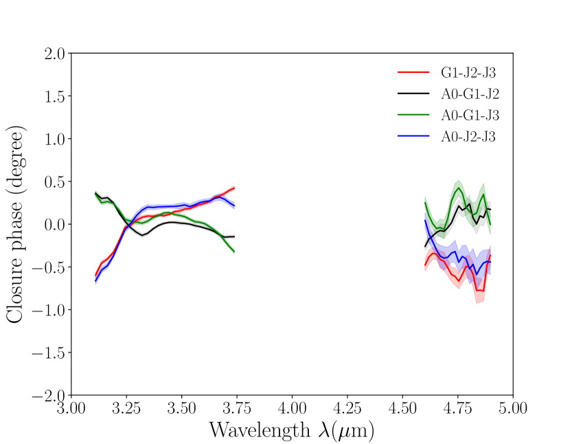
(a) #1 : $LM$ bands

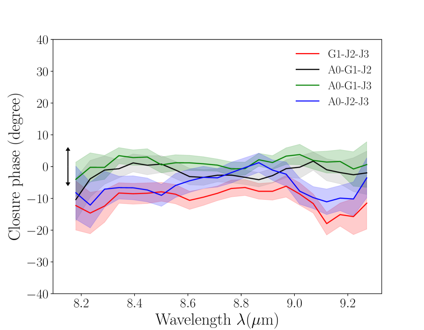
(b) #1 : $N$ band

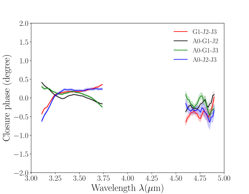
(c) #2 : $LM$ bands

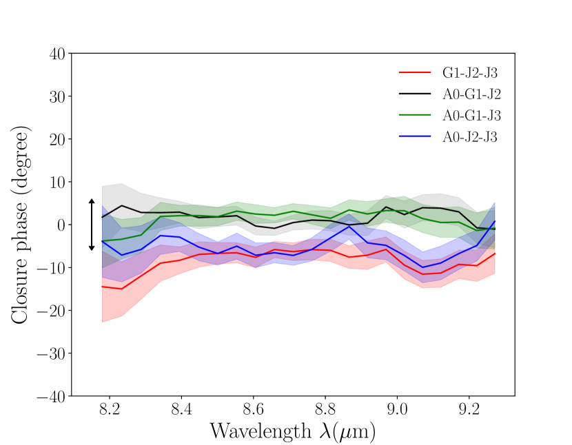
(d) #2 : $N$ band

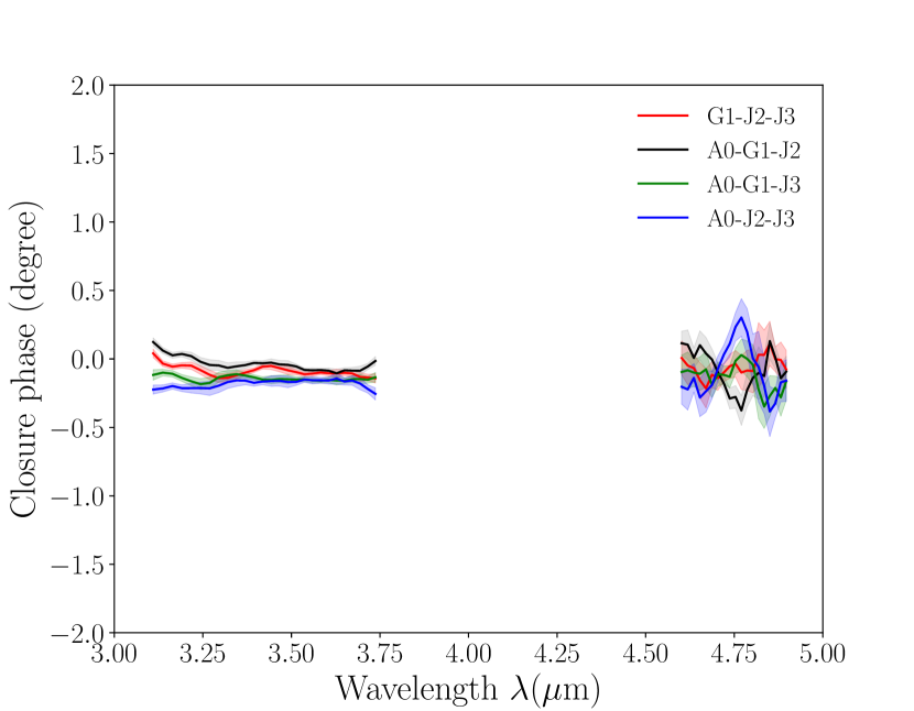
(e) #3 : $LM$ bands

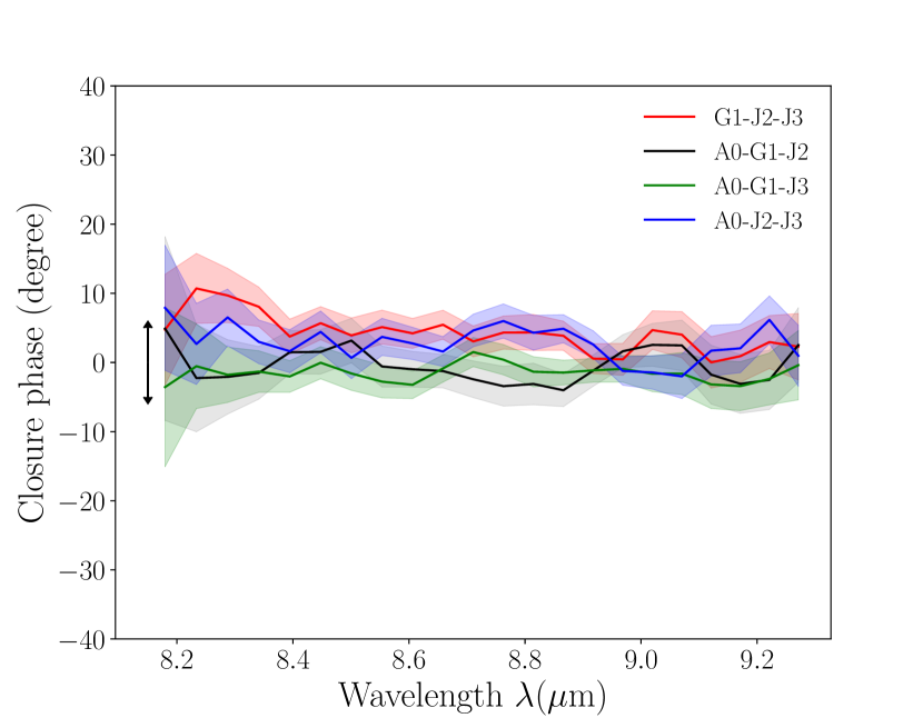
(f) #3 : $N$ band

Figure 3: Closure phase for observations #1, 2 and 3 for $LM$ and the $N$ bands for each ATs triplet. The double arrows in the $N$ band panels represent the typical peak-to-valley variation.

Figure 4: Averaged calibrated total flux for observations $\#1$, 2 and 3 in $LM$ bands plus the correlated flux in $N$ band for observation $\#3$. Panels (a) and (b) refer to $LM$ and $N$ bands respectively. SPIPS photosphere model is interpolated at the phase corresponding to the MATISSE the observation with parameters: $T_{\mathrm{eff}}(\phi_{\mathrm{obs}})$=$5014\pm 15\,$K; log $g(\phi_{\mathrm{obs}})$=$0.96\pm 0.10$; and $\theta_{\mathrm{UD}}(\phi_{\mathrm{obs}})$=$2.887\pm 0.003\,$mas. The Spitzer spectrum used in Sect. 2.2 is plotted for comparison.

3.2 Flux calibration

In $L$ and $M$ bands we calibrate the total flux $F_{\mathrm{tot,sci}}$ of $\ell$ Car using

$$F_{\mathrm{tot,sci}}=\frac{I_{\mathrm{tot,sci}}}{I_{\mathrm{tot,cal}}}\times F_{\mathrm{tot,cal}}$$ (2)

where $I_{\mathrm{tot,sci}}$ and $I_{\mathrm{tot,cal}}$ are the observed total raw flux of the science target and the calibrator respectively. $F_{\mathrm{tot,cal}}$ is the known flux of the standard star. We calibrate $\ell$ Car using standard stars with the closest air mass which are q Car and $\beta$ Vol for the observations of the first and second night respectively. $F_{\mathrm{tot,cal}}$ is given by their atmospheric templates from Cohen et al. (1999). Since the air mass of both target and calibrator are comparable we do not correct for the air mass. Moreover, while a chromatic correction exists for the $N$ band (Schütz & Sterzik 2005) it is not calibrated (to our knowledge) for the $L$ and $M$ bands. Then we average the three observations, adding uncertainties and systematics between each measurement in quadrature.

Since $\ell$ Car is too faint in $N$ band for accurate photometry (and thus absolute visibility) measurements, we use the correlated flux for the $N$ band, which is the flux contribution from the spatially unresolved structures of the source. We calibrated the correlated flux of the science target $F_{\mathrm{corr,sci}}$ following :

$$F_{\mathrm{corr,sci}}=\frac{I_{\mathrm{corr,sci}}}{I_{\mathrm{corr,cal}}}\times F_{\mathrm{tot,cal}}\times V_{\mathrm{cal}}$$ (3)

where $I_{\mathrm{corr,sci}}$ and $I_{\mathrm{corr,cal}}$ are the observed raw correlated flux of the science target and the calibrator respectively, and $V_{\mathrm{cal}}$ the calibrator visibility. For such an absolute calibration of the correlated flux, we need a robust interferometric calibrator with an atmospheric template given by Cohen et al. (1999). Only $\beta$ Vol, observed during the second night, meets these two requirements. Thus we only calibrate the correlated flux measurements from observation $\#3$ using the known flux of $\beta$ Vol. The calibrated correlated fluxes from the different baselines do not present any resolved features, allowing us to average the correlated flux from the different baselines. Note that we have discarded the spectral region between 9.3 and 10$\,\mu$m, due to the presence of a telluric ozone absorption feature around 9.6$\,\mu$m that strongly impacts the data quality. The calibrated total fluxes in $L$ and $M$ bands and the averaged calibrated $N$ band correlated flux are presented in Fig. 4.

We draw here several intermediate conclusions. First, the agreement between the measured flux with MATISSE, Spitzer and the SPIPS atmosphere model of $\ell$ Car is qualitatively satisfactory within the uncertainties. However, the MATISSE flux measurements have rather large uncertainties ($\geq$ 10%), making it difficult to determine the IR excess of $\ell$ Car with a precision at the few percent level. Secondly, we can see that the $N$ band correlated flux follows a pure Rayleigh-Jeans slope. This indicates the absence of silicate emission, which is consistent with the Spitzer data (Sect. 2.2). This is also in agreement with previous MIDI spectrum given by Kervella et al. (2009). Third, a resolved environment around $\ell$ Car is seen in the visibility measurements in the $L$ band. Indeed, the calibrated visibilities are significantly lower than the visibilities corresponding to a model of the star without CSE, as derived from the SPIPS algorithm at the specific phase of VLTI/MATISSE observations (see Fig. 2). Since the interferometric closure phase is zero the resolved structure around the star is centro-symmetric. In the next section we apply a centro-symmetric model of envelope on the observed $V^{2}$ measurements in $L$ band in order to investigate the diameter and flux contribution of the envelope.

4 Gaussian envelope model

In this section we fit a geometrical model on the measured $L$ band visibilities. $\ell$ Car and its CSE are modeled with an uniform disk (UD) and a surimposed Gaussian distribution, as in the previous studies on $\ell$ Car CSE (Kervella et al. 2006, 2009). The UD diameter corresponds to the one at the specific phase of the observation derived by SPIPS that is $\theta_{\mathrm{UD}}=2.887\pm 0.003\,$mas in the $L$ band. To model the CSE, we superimposed a Gaussian intensity distribution centered on the stellar disk. This CSE Gaussian model has two parameters which are the CSE diameter $\theta_{\mathrm{CSE}}$ taken as the Full Width at Half Maximum (FWHM), and the CSE flux contribution normalized to the total flux. We then performed a reduced $\chi_{r}^{2}$ fitting to adjust the total squared visibility of the model $V^{2}_{\mathrm{tot}}$ over the MATISSE observation in $L$ band. We computed the total squared visibility of the star plus CSE model using

$$V_{\mathrm{tot}}^{2}(f)=\Big{(}F_{\star}\,\left\lvert V_{\mathrm{UD}}(f)\right\rvert+F_{\mathrm{CSE}}\,\left\lvert V_{\mathrm{CSE}}(f)\right\rvert\Big{)}^{2}$$ (4)

where $f$=$B_{p}$/$\lambda$ is the spatial frequency ($B_{p}$ the length of the projected baseline), $F_{\star}$ and $F_{\mathrm{CSE}}$ are the normalized stellar and CSE flux contribution to the total flux respectively, normalized to unity $F_{\star}$ + $F_{\mathrm{CSE}}$ = 1. $V_{\mathrm{UD}}(f)$ is the visibility derived from the UD diameter of the star given by

$$V_{\mathrm{UD}}(f)=2\frac{J_{1}(\pi\theta_{\mathrm{UD}}f)}{\pi\theta_{\mathrm{UD}}f}$$ (5)

where $J_{1}$ is the Bessel function of the first order. $V_{\mathrm{CSE}}(f)$ is the visibility of a Gaussian intensity distribution

$$V_{\mathrm{CSE}}(f)=\exp\Big{[}-\frac{(\pi\theta_{\mathrm{CSE}}f)^{2}}{4\mathrm{ln}2}\Big{]}.$$ (6)

We perform the fit on observations $\#1$, 2 and 3 simultaneously, since $\ell$ Car is not expected to vary significantly between $\phi$=0.05 and 0.07. The derived visibility model is shown in Fig. 5 and we present the best-fit parameters in Table 4. The visibility model turns out to be consistent, within the error bars, with the three observations. However, the reduced $\chi_{r}^{2}$ is low (i.e. 0.2), thus the data are overfitted by the model and the uncertainties on the best-fit parameters are underestimated. In that case, to obtain more reliable uncertainties on the best-fit parameters we fit independently the three observations and we take the uncertainty as the standard deviation as of the resulted parameters. We resolve a CSE with a radius of 1.76$\pm 0.28\,R_{\star}$ accounting for about 7.0$\pm 1.4\%$ of the flux contribution in the $L$ band, that gives an IR excess of $-$0.07 mag. Both the size and the flux contribution are in agreement with previous studies which have found a compact environment of size 1.9$\pm$1.4$\,R_{\star}$ in $K$ band with VINCI and 3.0$\pm$1.1$\,R_{\star}$ in $N$ band with MIDI (Kervella et al. 2006), with few percents in flux contribution in both cases. As noted by Kervella et al. (2006), the large uncertainties in the $K$ band diameter is due to a lack of interferometric data for baselines between 15 to 75 m. We also note that cycle-to-cycle amplitude variations discovered in $\ell$ Car (Anderson 2014; Anderson et al. 2016) could slightly affect the diameter in the $K$ band. On the other hand Kervella et al. (2009) found extended emission between 100 and 1000 AU ($\approx$100-1000$\,R_{\star}$) using MIDI and VISIR observations in the $N$ band. Thus it is possible that the CSE have both a compact and an extended component which are observable at different wavelengths. The CSE flux contribution of 7% is also in agreement with the MATISSE total flux within the uncertainties (see Fig. 4), as well as the determined IR excess of about $-$0.05 to $-$0.1 mag we derived from Fig. 1(b) in Sect. 2.2.

Table 4: Fitted parameters of a Gaussian CSE with flux contribution $F_{\mathrm{CSE}}(\%)$ and FWHM $\theta_{\mathrm{CSE}}$(mas) which is also expressed in stellar radius $R_{\mathrm{CSE}}$($R_{\star}$). Parameters $F_{\mathrm{CSE}}$ and $\theta_{\mathrm{CSE}}$ are weakly correlated with a correlation coefficient of 0.09. The uncertainties on the parameters are obtained using the standard deviation of the best-fit parameters for the three observations fitted independently. These results are compared with those obtained with VINCI in $K$ band and MIDI in $N$ band from Kervella et al. (2006).

	This work	VINCI	MIDI
	$L$	$K$	$N$
$f_{\mathrm{CSE}}(\%)$	7.0$\pm$1.4	4.2$\pm$0.2	-
$\theta_{\mathrm{CSE}}$(mas)	5.06$\pm$0.81	5.8$\pm$4.5	8.0$\pm$3.0
$R_{\mathrm{CSE}}$($R_{\star}$)	1.76$\pm$0.28	1.9$\pm$1.4	3.0$\pm$1.1
$\chi_{r}^{2}$	0.2	0.65	-

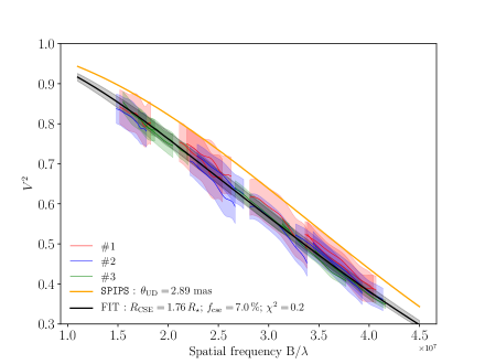
Figure 5: Fitted Gaussian CSE around $\ell$ Car for the combined observations $\#1$, 2 and 3 in the $L$ band. The error on the visibility model is obtained using the covariance matrix of the fitting result.

5 Physical origin of the IR excess

5.1 Dust envelope

The absence of emission features in the $N$ band in both MATISSE and Spitzer spectra rules out the presence of dust from typical oxygen rich star mineralogy with amorphous silicates or aluminum oxide, which present a characteristic spectral shape in $N$ band. A pure iron envelope, which presents a continuum emission, is also unlikely to be created. We already considered then rejected these possibilities in Paper I (see the Figures 8 and 9 in it). We note that the presence of large grains of silicate, with a size of about 1$\,\mu$m and more, would lead to a broader emission which could completely disappear (Henning 2010). However the reason why large grains would preferentially be created in the envelope of Cepheids remains to be explained. In addition, considering the best-fit of the Gaussian CSE model, at a distance of 1.76$\,R_{\star}$ from the stellar center, i.e. 0.76$\,R_{\star}$ from the photosphere, the temperature would exceed 2000 K, therefore dust cannot survive since it would sublimate (Gail & Sedlmayr 1999). These physical difficulties to reproduce the IR excess with dust envelopes were also recently pointed out by Groenewegen (2020) who fitted the SEDs of 477 Cepheids (including $\ell$ Car) with a dust radiative transfer code.

5.2 A thin shell of ionized gas

In Paper I we suggested the presence of a thin shell of ionized gas, with a radius of about 1.15$\,R_{\star}$, to explain the reconstructed IR excess of five Cepheids. We use the same model for $\ell$ Car with a shell of ionized gas, to test its consistency with IR excess and interferometric observations. In this part we perform a reduced $\chi_{r}^{2}$ fitting of the shell parameters on the IR excess reconstructed in Sect. 2.2. This simple model has three physical parameters which are: the shell radius; the temperature; and the mass of ionized gas. An additional parameter is applied as an offset to the whole reconstructed IR excess from Fig. 1(b), allowing the model to present either a deficit or an excess in the visible domain if necessary. Indeed, the key point is when considering a shell of ionized gas, this shell is expected to absorb the light coming from the star in the visible domain, which is currently not considered in the SPIPS algorithm when reconstructing the IR excess (the $V$ magnitude is forced to be zero, see Fig. 1(a)). However, thanks to the VLTI/MATISSE measurements of flux contribution of the CSE in the $L$ band (7%), we can fix this offset parameter consistently to 0.03 magnitude, to force the IR excess in $L$ band from SPIPS (that is $\approx$10%) to be also 7%, within the uncertainties. We present the result of the modeling ($\chi_{r}^{2}$=0.55) constrained by the spectrum of $\ell$ Car in Fig. 6. We find a thin shell radius of $R_{\mathrm{shell}}$=1.13$\pm 0.02\,R_{\star}$ which is lower than the Gaussian CSE of 1.76$\pm 0.28\,R_{\star}$ constrained by MATISSE observations. On the other hand this model also reproduces the Spitzer spectrum better than the SPIPS predicted photometries. In particular its value in the $L$ band is about 1% (see Fig. 6) which is not consistent with the value derived using $L$ band visibilities ($\sim 7$%). This model has also derived weak near-infrared excess for several stars in Paper I (see its Figure 11). This behaviour is physically explained by the free-bound absorption of hydrogen before the free-free emission dominates at longer wavelength. We have explored the spatial parameters to test if a larger ionized envelope has the potential to match MATISSE observations with the IR excess. However, our model is not able to accurately reproduce all the observations. Also, even if our model is complex considering the physics involved (free-free and bound-free opacities description), its geometrical description is rather simple, with a constant density and temperature distribution. Thus, it might not be adapted to the modeling of a larger envelope.

5.3 Limit of the model

The derived parameters of the shell of ionized gas depend on the initial IR excess derived by SPIPS. Any systematics in this calculation could in turn affect the IR excess and the parameters of the shell of ionized gas. As noted by Hocdé et al. (2020b), the derived distance of SPIPS would be systematically affected if the shell of ionized gas is not taken into account, because of its absorption in the visible. This systematic should be only few percents ($10^{\Delta\mathrm{m}/2.5}$) all parameters being unchanged. The direct implementation of the gas model into the SPIPS fitting has to be tested in forthcoming studies to correct this uncertainty. Moreover, Gallenne et al. 2021 (submitted) studied the ad-hoc IR excess derived by SPIPS for a larger sample of stars and found that angular diameter and the colour excess are the most impacted parameters when no ad-hoc IR excess model is included. However in the case of $\ell$ Car these parameters appear to be well constrained by angular diameter measurements, the reddening and the distance are also in agreement with values found in the literature (see Appendix A).

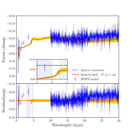
Figure 6: $\ell$ Car IR excess fitting result of ionized gas shell following the method described in Paper I. Yellow region is the error on the magnitude obtained using the covariance matrix of the fitting result. We find a thin shell of ionized gas with radius $R_{\mathrm{shell}}$=1.13$\pm$0.02$\,R_{\star}$; temperature $T_{\mathrm{shell}}$=3791$\pm$85$\,K$; mass of ionized gas $M$=9.10$\times 10^{-8}\pm$8.5$\times 10^{-9}\,$$\mathrm{M}_{\odot}\,$, using an ad-hoc offset of +0.03 mag on the data in order to match the IR excess found by VLTI/MATISSE and the one of SPIPS (see the text); and $\chi_{r}^{2}$=0.55. The subplot shows the comparison between the flux contribution derived from the Gaussian CSE (dashed line), the IR excess from SPIPS (red point) and IR excess from a shell of ionized gas in the $LM$ band (red line).

5.4 Perspectives

An interesting physical alternative is to consider free-free emission produced by negative hydrogen ion H^-, with free electrons provided by metals. Indeed for an envelope of 2$\,R_{\star}$ the average temperature is about 3000 K and the hydrogen is neutral. Thus, in that case, most of the free electrons would be provided by silicon, iron and magnesium which have a mean first ionization potential of 7.89 eV. As neutral hydrogen is able to form negative hydrogen ion, H^- could generate an infrared excess with free-free emission. This phenomenon is known to produce a significant IR excess compared to dust emission in the extended chromosphere of cool supergiant stars such as Betelgeuse (Gilman 1974; Humphreys 1974; Lambert & Snell 1975; Altenhoff et al. 1979; Skinner & Whitmore 1987). Moreover, the photo-detachment potential occurs at 1.6$\,\mu$m for the H^- mechanism, thus free-free emission should dominate the IR excess above this wavelength, as it is suggested by the SPIPS cycle-averaged IR excess. This single photo-detachment has also the advantage to avoid the important bound-free absorption in the near-infrared produced in the preceding model. We thus suggest that the compact structure we resolved around $\ell$ Car has the potential to produce IR excess through H^- free-free mechanism by analogy with extended chromosphere of cool supergiant stars. Further investigations are necessary to confirm this hypothesis.

6 Conclusions

Determining the nature and the occurrence of the CSEs of Cepheids is of high interest to quantify their impact on the Period-Luminosity relation, and also for understanding the mass-loss mechanisms at play. In this paper, we constrain both the IR excess and the geometry of the CSE of $\ell$ Car using both Spitzer low-resolution spectroscopy and MATISSE interferometric observations in the mid-infrared. Assuming an IR excess ad-hoc model, we used SPIPS to derive the photospheric parameters of the star in order to compare with Spitzer and MATISSE at their respective phase of observation. This analysis allows to derive the IR excess from Spitzer and also to derive the CSE properties in the $L$ band spatially resolved with MATISSE. These observations lead to the following conclusions on the physical nature of $\ell$ Car’s CSE:

1. We resolve a centro-symmetric and compact structure in the $L$ band with VLTI/MATISSE that has a radius of about 1.76$\,R_{\star}$. The flux contribution is about 7%.

2. We find no clear evidence for dust emission features around 10$\,\mu$m ($N$ band) in MATISSE and Spitzer spectra which suggests an absence of circumstellar dust.

3. Our dedicated model of shell of ionized gas better reproduces the mid-infrared Spitzer spectrum and implies a size for the CSE lower than the one derived from VLTI/MATISSE observations (1.13$\pm 0.02\,R_{\star}$ versus $1.76\pm$0.28$\,R_{\star}$), as well as a lower flux in the $L$ band (1% versus 7%).

4. We suggest that improving our model of shell of ionized gas by including the free-free emission from negative hydrogen ion would probably help reproducing the observations, i.e. the size of the CSE and the IR excess, in particular in the $L$ band.

While the compact CSE of $\ell$ Car is likely gaseous, the exact physical origin of the IR excess remains uncertain. Further observations of Cepheids depending on both their pulsation period and their location in the HR diagram are necessary to understand the CSE’s IR excess. This could be a key to unbias Period-Luminosity relation from Cepheids IR excess.

Appendix A SPIPS data set and fitted pulsational model of the star sample.

Figure 7 is organized as follows: pulsational velocity, effective temperature and angular diameter curves according to the pulsation phase are shown on the left panels, while the right panels display photometric data in various bands. Above the figure, the projection factor set to $p=1.270$ is indicated, along with the fitted distance $d$ using parallax-of-pulsation method, the fitted color excess E($B-V$), and the ad-hoc IR excess law. In this work we arbitrarily set the p-factor to 1.27 following the general agreement around this value for several stars in the literature (Nardetto et al. 2004; Mérand et al. 2005; Nardetto et al. 2009). However, there is no agreement for the optimum value to use, and it is also the case for $\ell$ Car. In the case of this star (Nardetto et al. 2007, 2009) found a p-factor of 1.28$\pm$0.02 and 1.22$\pm$0.04 using different observational techniques which both are in agreement with 1.27 within about 1 sigma. Thus, a possible systematic cannot be excluded although the distance derived by SPIPS ($d=519.2\pm 4.5\,$pc) is in agreement for example with the distance obtained using Gaia parallaxes (505$\pm$28 pc) (Gaia Collaboration et al. 2018) or the one derived using a recent period-luminosity calibrated for Cepheids in the Milky Way (544$\pm$32 pc) (Breuval et al. 2020).

Gallenne et al. (2021, submitted) have shown that the absence of IR excess model in the SPIPS fit can affect the derivation of the angular diameter and the colour excess. In our fit using IR excess model, we emphasize the good agreement of the angular diameter model with the data (panel b), and also the consistency of the derived colour excess with the one given by Stilism 3D extinction map (Capitanio et al. 2017), that is $0.148\pm 0.006$ versus $0.116\pm 0.26$. In the photometric panels, the gray dashed line corresponds to the magnitude of the SPIPS model without CSE. It actually corresponds to the magnitude of a Kurucz atmosphere model, $m_{\mathrm{kurucz}}$, obtained with the ATLAS9 simulation code from Castelli & Kurucz (2003), with solar metallicity and a standard turbulent velocity of 2 km/s. These models are indeed suitable for deriving precise synthetic photometry (Castelli 1999), in comparison with MARCS models giving rough flux estimates. The gray line corresponds to the best SPIPS model, which is composed of the latter model without CSE plus an IR excess model. In the angular diameter panels, the gray curve corresponds to limb-darkened (LD) angular diameters. For stars with solar metallicity, when effective temperature is low enough, CO molecules can form in the photosphere and absorb light in the CO band-head at 4.6 $\mu m$ (Scowcroft et al. 2016). This effect is observed in the Spitzer I2 IRAC dataset. In this case, these data were ignored during the fitting of SPIPS. Panels presenting a horizontal blue bar contain only one data with undetermined phase of observation, thus these photometric mid-infrared bands were not used in the IR excess reconstruction in Sect. 2.1 and 2.2

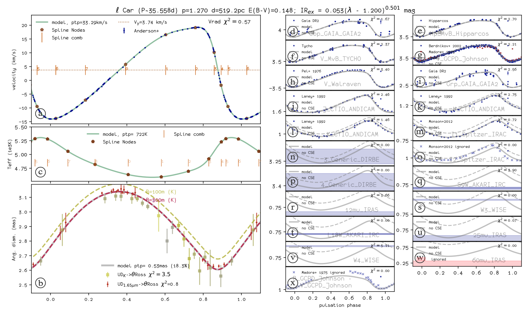
Figure 7: The SPIPS results of $\ell$ Car. Velocity: Anderson (2014). Effective temperature: No data. Angular diameter: Kervella et al. (2006). Photometry: Madore (1975), Pel (1976), Neugebauer et al. (1984), Laney & Stobie (1992), ESA (1997), Berdnikov & Turner (2002), Smith et al. (2004), Ammons et al. (2006), Wright et al. (2010), Ishihara et al. (2010), Monson et al. (2012), Gaia Collaboration et al. (2018).

Appendix B Verification of the diameters of the calibrators

In order to verify the consistency of the standard stars of the first night (27 February), we consider all calibrators available during the night (B Cen, e Cen, $\epsilon$ Ant) and we inter-calibrate them. Thus, each calibrator is calibrated using the two others. We performed six different calibrations in total, following Table 5 and Fig. 8. The results are also compared with the known values from the literature.

From these results, the diameters of $\epsilon$ Ant and e Cen are in excellent agreement with those given by the JSDC when they are calibrated from one to another, and the visibilities are well fitted by an uniform disk (UD) model (see Figures 8(a) and 8(b)). On the contrary, we find important inconsistencies when deriving the diameter of B Cen or using it as a calibrator (see Figures 8(c), 8(d), 8(e) and 8(f)). In particular this standard star is suspected to be 20$\%$ larger tan the diameter given by the JSDC ($\approx\,$3 mas instead of 2.5 mas). Moreover, a simple UD model seems to be unsuitable for fitting the observed visibilities (see black curve in Figures 8(e) and 8(f)). On the other hand the diameter of B Cen is also well established by interferometry in the $K$ band (Richichi et al. 2009) and was used many times as an interferometric calibrator (Kervella et al. 2006; Kervella 2007). We emphasize that the transfer function was very stable during this night, thus this result cannot be attributed to the atmospheric conditions (see coherence time in Table 2). Since the origin of this discrepancy remains unknown, this analysis prevented us for using B Cen to calibrate the Cepheid $\ell$ Car.

Table 5: Diameters in milliarcseconds obtained by the inter-calibration between B Cen, $\epsilon$ Ant and e Cen. The targets of the calibration are indicated in the upper part of the table together with their angular diameter in $L$ band from the JSDC catalogue in parentheses. The first column indicates the calibrator used to obtain the derived UD angular diameters in each cell. The red cells represent discrepant values compared to the JSDC catalogue at more than 1$\,\sigma$. This deviation from the derived $\theta_{\mathrm{UD}}$ to the JSDC value is derived by $|\theta_{\mathrm{UD}}-\leavevmode\nobreak\ \theta_{\mathrm{JSDC}}|/\sigma_{\mathrm{JSDC}}$.

	e Cen	$\epsilon$ Ant	B Cen
	(2.97$\pm$0.29)	(2.86$\pm$0.30)	(2.54$\pm$0.28)
e Cen	-	2.91$\pm$0.01	red!25 3.09$\pm$0.02
$\epsilon$ Ant	2.96$\pm$0.01	-	red!25 3.10$\pm$0.02
B Cen	red!25 2.41$\pm$0.02	red!25 2.39$\pm$0.02	-

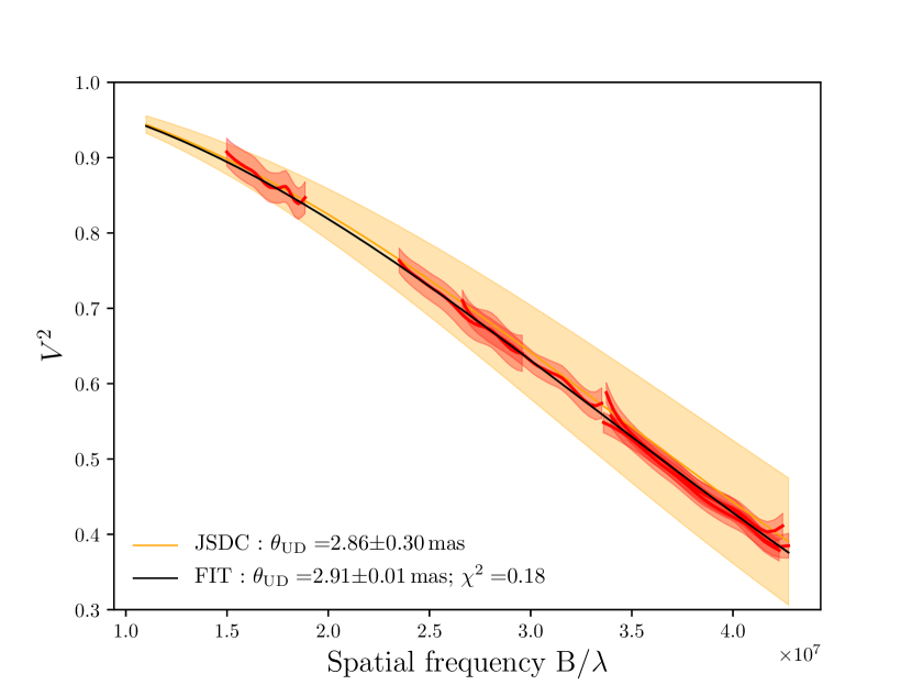
(a) $\epsilon$ Ant calibrated with e Cen

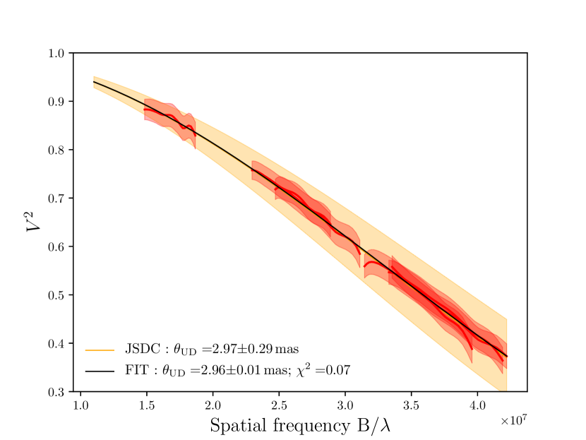
(b) e Cen calibrated with $\epsilon$ Ant

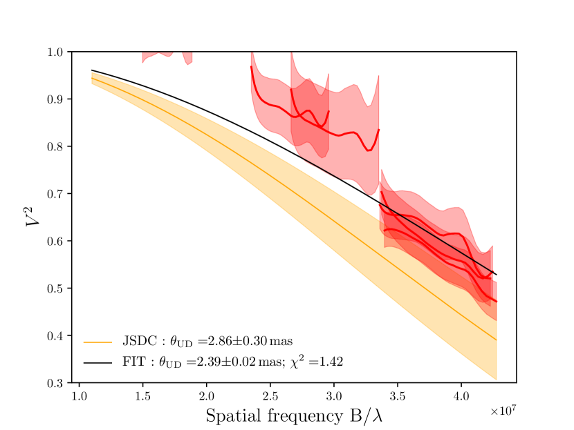
(c) $\epsilon$ Ant calibrated with B Cen

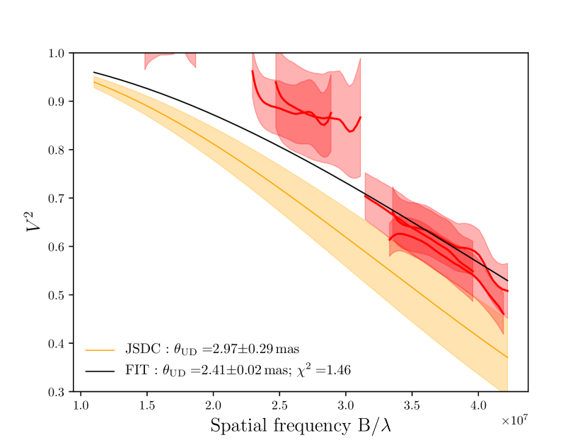
(d) e Cen calibrated with B Cen

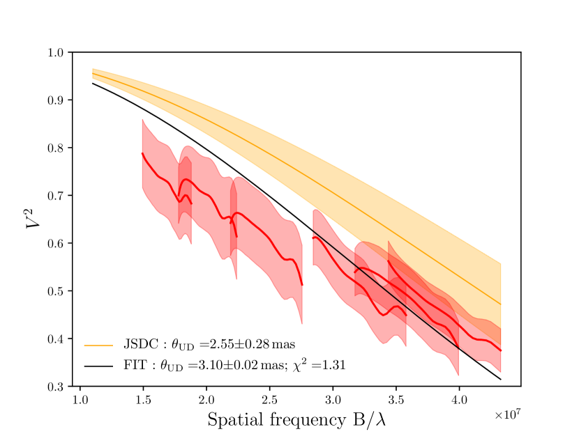
(e) B Cen calibrated with $\epsilon$ Ant

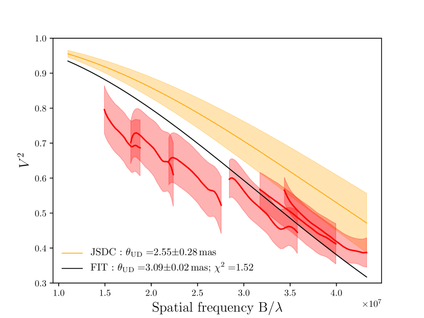
(f) B Cen calibrated with e Cen

Figure 8: Inter-calibration of the different calibrators and comparison with JSDC diameters. (a) and (b) : $\epsilon$ Ant and e Cen diameters are in agreement with the JSDC when they are calibrated from each other. (c) and (d) : On the contrary the diameter of $\epsilon$ Ant and e Cen are inconsistent with the JSDC catalogue when they are calibrated with B Cen. (e) and (f) : B Cen diameter is inconsistent with the JSDC catalogue.