Synthetic RGB photometry of bright stars: definition of the standard photometric system and UCM library of spectrophotometric spectra

Abstract

Although the use of RGB photometry has exploded in the last decades due to the advent of high-quality and inexpensive digital cameras equipped with Bayer-like color filter systems, there is surprisingly no catalogue of bright stars that can be used for calibration purposes. Since due to their excessive brightness, accurate enough spectrophotometric measurements of bright stars typically cannot be performed with modern large telescopes, we have employed historical 13-color medium-narrow-band photometric data, gathered with quite reliable photomultipliers, to fit the spectrum of 1346 bright stars using stellar atmosphere models. This not only constitutes a useful compilation of bright spectrophotometric standards well spread in the celestial sphere, the UCM library of spectrophotometric spectra, but allows the generation of a catalogue of reference RGB magnitudes, with typical random uncertainties $\sim 0.01$ mag. For that purpose, we have defined a new set of spectral sensitivity curves, computed as the median of 28 sets of empirical sensitivity curves from the literature, that can be used to establish a standard RGB photometric system. Conversions between RGB magnitudes computed with any of these sets of empirical RGB curves and those determined with the new standard photometric system are provided. Even though particular RGB measurements from single cameras are not expected to provide extremely accurate photometric data, the repeatability and multiplicity of observations will allow access to a large amount of exploitable data in many astronomical fields, such as the detailed monitoring of light pollution and its impact on the night sky brightness, or the study of meteors, solar system bodies, variable stars, and transient objects. In addition, the RGB magnitudes presented here make the sky an accessible and free laboratory for the calibration of the cameras themselves.

1 Introduction

Scientific and commercial-grade RGB cameras provide affordable means for the acquisition of quantitative radiance data with large fields-of-view, using a large number of pixels, and moderate multispectral content. Manufactured with different technologies, and widely different in terms of their absolute sensitivities, noise levels, pixel sizes and processing capabilities, all of them share the key common feature of detecting light in three spectral channels broadly comparable across devices, centered in the red, green, and blue regions of the visible spectrum, providing that way a relatively homogenous basis for data sharing and processing.

The sustained improvement in the performance of the CCD and CMOS RGB sensor arrays enabled the development of an increasing number of scientific applications in astronomy, by both the professional and amateur communities, which is expected to grow in the coming years. Among other examples, commercial-grade RGB cameras have proven to be valuable science tools for night sky brightness measurement (Hänel et al., 2018; Jechow et al., 2018; Bertolo et al., 2019; Jechow et al., 2019a, b; Jechow, 2019; Jechow & Hölker, 2019; Kolláth et al., 2020), radiometry of artificial light polluting sources from Earth-orbit platforms (Kyba et al., 2014; Stefanov et al., 2017; Zheng et al., 2018; Sánchez de Miguel et al., 2019; Sánchez de Miguel et al., 2020), as well as from airborne (Kuechly et al., 2012; Bouroussis & Topalis, 2020), and ground based stations (Dobler et al., 2015; Meier, 2018; Bará et al., 2019), meteor and fireball detection (Gural & Šegon, 2009), planetary astronomy (Mousis et al., 2014), and variable stars (Blackford, 2016).

Besides, the exponential growth of the consumer optoelectronics segment opens unprecedented opportunities for large-scale citizen science projects (see e.g. Kyba, 2019; Zamorano, 2020): recent market studies (Nisselson et al., 2017) estimate that by 2022 as much as 45 billion cameras (defined as the combination of an objective lens plus a focal plane spatially resolved sensor) will be operative worldwide in different supports, from hand-held smartphones and classical photographic units to home appliances and artificial vision systems.

Despite these facts, a consistent astronomical magnitude system has not yet been defined for RGB photometry. The possibility of reporting fluxes (irradiances) in astronomical magnitudes, and surface brightnesses (radiances) in magnitudes per square arcsecond in the native photometric bands of these widely used devices is appealing. The relative similarity of the $R$, $G$, and $B$ channels across camera models, and their expected stability in the foreseeable future (as far as cameras continue to be developed for human vision-driven applications) are two key features enabling large-scale broadly-homogeneous data gathering and monitoring across extended periods of time.

We develop in this work a complete RGB photometric system, characterized by a set of basic filters, the use of photon-based quantities, and with zero points defined in the absolute (AB) scale. We also provide a catalogue of RGB star magnitudes corresponding to a good subset of the brightest stars in the celestial sphere, that can be used as a reference for calibration purposes. The focus on the bright stars comes from the need to provide observers using wide-field digital cameras with the possibility of properly calibrating their images, even with short exposure times. The goal is to reach the same level of calibration accuracy attained in radiometric measurements performed in laboratory within the optical range (see Wolfe, 1998, Table 10-4): 1–2.5% with tungsten lamps, or even 0.1% with self-calibrating detectors.

The absolute spectrophotometric flux calibration of bright star spectra is not an easy task with modern large telescopes and spectrographs, mainly due to the difficulty to avoid light losses while preserving the desired spectral resolutions using narrow slits, but also because of other observational problems like avoiding detector saturation or lack of linearity of the detectors themselves when used at very high count rates, the proper correction of atmospheric extinction or differential refraction (when observing at non-negligible airmasses, with the slit position angle different from the parallactic angle, while covering relatively wide wavelength ranges), or the inhomogeneous illumination of the spectrograph focal plane in very short exposure times due to the limited speed of camera shutters, to mention a few. Although the use of neutral density filters can help to alleviate some of these problems, this approach not only requires a good spectrophotometric calibration of the density filters themselves, but also translates into using modern telescopes to observe bright stars with large exposure times, something that typically is not easy to get approved by telescope allocation committees.

For all those reasons we decided to base our work on historical, but quite reliable and homogeneous, medium-narrow-band photometric data, that can be used to fit star model spectra able reproduce the observed spectral energy distribution of bright stars. The fitted models have then been used to compute synthetic RGB magnitudes, fulfilling our initial goal.

A brief description of the practical computation of synthetic magnitudes followed in this work is summarised in Section 2. Section 3 describes the photometric data and initial sample selection, while the model fitting procedure and final sample definition, based on comparisons between synthetic magnitudes and additional photometric measurements, are presented in Section 4. To avoid the problem of choosing the RGB sensitivity curves of a particular camera, we decided to define a set of reference RGB spectral sensitivity curves, using median values from existing sensitivity curves of well-known cameras, that can be used to establish an RGB standard photometric system. The definition of these curves is presented in Section 5, together with the RGB magnitudes for the 1346 stars constituting the UCM library of spectrophotometric standards, and a discussion concerning the conversion between magnitudes measured under the standard RGB system defined here and those derived employing the RGB sensitivity curves of individual cameras. The conclusions of this work are summarized in Section 6, while Appendices A and B include the graphical comparison of the results of applying the adopted fitting technique in 39 stars with available spectrophotometric data from the literature, and a table with polynomial coefficients that allow the computation of the expected differences between the standard RGB system and 28 particular digital cameras, respectively.

2 Computation of synthetic magnitudes

Synthetic magnitudes in this work have been determined using the Python package synphot (STScI development Team, 2018), which facilitates the computation of photometric properties from user-defined bandpasses and spectra. This package follows the photon-counting formalism, expected for modern CCD detectors (see e.g. Casagrande & VandenBerg, 2014), where the number of photons, instead of the arriving energy, is the relevant property to be considered. In this way, for a particular bandpass defined in the wavelength interval ranging from $\lambda_{i}$ to $\lambda_{f}$, magnitudes are computed following

$$m=-2.5\,\log_{10}\frac{\int_{\lambda_{i}}^{\lambda_{f}}n_{\gamma}(\lambda)\;T(\lambda)\;{\rm d}\lambda}{\int_{\lambda_{i}}^{\lambda_{f}}n_{\gamma,r}(\lambda)\;T(\lambda)\;{\rm d}\lambda}=-2.5\,\log_{10}\frac{N_{\gamma}}{N_{\gamma,r}},$$ (1)

where $n_{\gamma}(\lambda)$ is the number of photons per unit time and per unit spectral bandwidth at the wavelength $\lambda$ through a unit area (photons s^-1 cm^-2 Å^-1; flux units known as PHOTLAM in synphot) for the desired target. Similarly, $n_{\gamma,r}(\lambda)$ has the same physical meaning for the spectrum to be used to set the $m\!=\!0$ reference point. In addition, $T(\lambda)$ is the system spectral sensitivity response. Sometimes, it is also useful to compute $N_{\gamma}$, the integrated number of photons (photons s^-1 cm^-2) within the bandpass, modulated by the spectral sensitivity response, although logically the absolute number depends on the particular normalization of $T(\lambda)$. In this sense, it is important to note that if the averaged number of photons within the bandpass is the sought parameter, a proper normalization must be performed using $T(\lambda)$ as the weighting factor

$$\langle n_{\gamma}\rangle=\frac{\int_{\lambda_{i}}^{\lambda_{f}}n_{\gamma}(\lambda)\;T(\lambda)\;{\rm d}\lambda}{\int_{\lambda_{i}}^{\lambda_{f}}T(\lambda)\;{\rm d}\lambda}=\frac{N_{\gamma}}{\int_{\lambda_{i}}^{\lambda_{f}}T(\lambda)\;{\rm d}\lambda},$$ (2)

with a similar expression for the reference spectrum $\langle n_{\gamma,r}\rangle$, interchanging $n_{\gamma}(\lambda)$ by $n_{\gamma,r}(\lambda)$, and $N_{\gamma}$ by $N_{\gamma,r}$, in the above equation. The denominator of the last equation, that works as normalization factor and is computed in synphot as the bandpass equivalent width, is actually also present in both the numerator and denominator of Eq. 1, but cancels out and does not appear explicitly.

Since the number of photons is directly related to the incoming flux densities, magnitudes can also be computed as

$$m=-2.5\,\log_{10}\frac{\int_{\lambda_{i}}^{\lambda_{f}}f(\lambda)\;\frac{\lambda}{h\,c}\;T(\lambda)\;{\rm d}\lambda}{\int_{\lambda_{i}}^{\lambda_{f}}f_{r}(\lambda)\;\frac{\lambda}{h\,c}\;T(\lambda)\;{\rm d}\lambda},$$ (3)

being $f(\lambda)$ the flux density of the target (erg s^-1 cm^-2 Å^-1; flux units known as FLAM in synphot), and $f_{r}(\lambda)$ the flux density of the reference spectrum. In this case, we have not simplified the $h\,c$ factor in the last equation in order to keep the traceability of the units involved, being both the numerator and denominator in that fraction given in photons s^-1 cm^-2.

We have checked that the computed synthetic magnitudes with synphot agree with the measurements performed with pyphot, another Python package providing tools to compute synthetic photometry. In no case the differences found were larger than 0.0002 mag. In addition, we also performed our own integrations by directly programming the equations shown in this section, using trapezoidal integrations with the Numpy function trapz, being the largest differences also smaller than 0.0002 mag. However, it is worth noticing that when applying a different integration strategy, namely the Simpson’s rule with the scipy function simpson, the differences are slightly larger, reaching in some cases 0.01 mag. Since the Simpson’s rule approximates the original function using piecewise quadratic functions, it is clear that this fact has a non-negligible effect on the computations. For that reason, we advocate the use of synphot or pyphot, when delegating in third-party software packages when computing synthetic magnitudes, or the implementation of the simple trapezoidal integration, when employing user-defined code.

3 Data sample

3.1 Historical 13-color photometric data

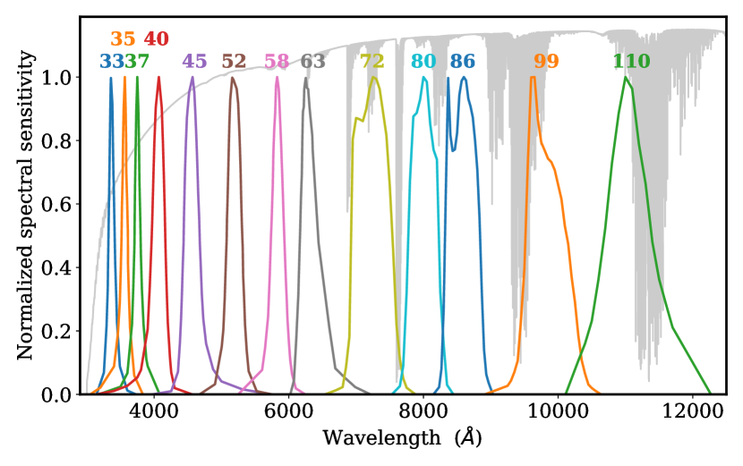
Figure 1: Spectral sensitivity curves for the 13 filters, as given by Johnson & Mitchell (1975, see their Table 1). The name of each filter indicates its approximate effective wavelength. Just for illustration, we are also displaying the atmospheric telluric absorption (upper gray line) computed with the help of the ESO SKYCALC tool (Moehler et al., 2014).

Table 1: Basic properties of the filters composing the 13C photometric system: (1) filter identification, (2) bandpass average wavelength, (3) equivalent width, and (4) full width at half maximum.

Filter	$\lambda_{0}$ (Å)	Equivalent width (Å)	FWHM (Å)
33	3374	116	143
35	3540	132	224
37	3749	133	213
40	4034	240	349
45	4603	285	383
52	5187	259	250
58	5822	230	247
63	6360	326	392
72	7239	589	463
80	8002	435	348
86	8585	483	380
99	9828	583	575
110	11088	830	872

The classical 13-color (hereafter 13C) medium-narrow-band photometric system (Johnson et al., 1967; Mitchell & Johnson, 1969; Johnson & Mitchell, 1975; Schuster, 1982b) was created with the aim to obtain homogeneous and calibrated photometric measurements of bright stars, with a high level of accuracy. Each filter is identified by a number that indicates its approximate effective wavelength. The spectral sensitivity curves for all the filters are displayed in Fig. 1, whereas some basic filter properties are provided in Table 1. The seven bluest filters, with effective wavelengths ranging from 3370 Å to 5820 Å, provided quantitative information concerning the behaviour of the continuum of early-type stars, including the Balmer jump. The six reddest filters, covering the 6360 Å to 11090 Å region, were selected to avoid conspicuous telluric atmospheric features.

Apart from the initial references, the usefulness of the 13C photometric system was clearly demonstrated through numerous stellar studies derived from its use (see e.g. Schuster, 1976; Alvarez & Schuster, 1978; Schuster, 1979a, b, c; Marx & Lehmann, 1979; Chavarria-K. & de Lara, 1981; Schuster, 1982a, b; Alvarez & Schuster, 1982; Schuster & Alvarez, 1983; Schuster, 1984; Schuster & Guichard, 1984; Conconi & Mantegazza, 1985; Schuster & Guichard, 1985; Petford & Blackwell, 1989; Bravo Alfaro et al., 1993, 1997, and references therein).

3.2 The star sample

We have assembled 13C photometric data of bright stars, belonging to the Bright Star Catalog (Hoffleit, 1964), coming from three different sources: 1380 stars from Johnson & Mitchell (1975, hereafter JM75), 81 stars from Schuster (1976, hereafter S76), and 71 stars from Bravo Alfaro et al. (1997, hereafter BAS97). The largest contribution comes from the JM75 sample, that basically covered all the stars brighter than the fifth visual magnitude north of declination $-20^{\degr}$, and most of the stars brighter than the fourth visual magnitude below that declination. It is important to note that 163 stars from the JM75 sample ($\sim 12$% of the objects) do not have photometric data for the 5 reddest filters (72, 80, 86, 99 and 110). On the other hand, the S76 and BAS97 samples correspond to solar-type and A0-K0 supergiant stars, respectively. Taking into account that there are one and nine stars in common between JM75 and S76, and between JM75 and BAS97, respectively, the total initial number of different stars is 1522. As explained later (Sect. 4.3), the initial list was cleaned by removing stars with poor results in the fitting process or by discrepancies with the available Johnson $B$ and $V$ photometric data retrieved from the Simbad database. The final sample, listed in Table 2, comprises a total of 1346 stars, with a magnitude distribution as shown in Fig. 2, being the stars well spread over the whole celestial sphere, as displayed in Fig. 3.

Figure 2: Distribution of the final star selection according to the stellar magnitude in the 52 filter. The number of stars belonging to each source is displayed between parenthesis in the figure key. The red line delineates the coadded histogram. It is clear that most of the stars come from JM75, with a small contribution of S76 and BAS97 in the faint regime of the sample.

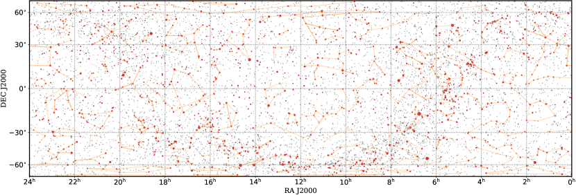
Figure 3: Lambert cylindrical equal-area projection in J2000 equatorial coordinates showing the distribution of the stars belonging to the Bright Star Catalog (Hoffleit, 1964). The 1346 stars composing the UCM library of spectrophotometric standards are highlighted as red filled cicles. Simple constellations shapes (van der Sluys, 2005), displayed with light orange lines, are also shown to facilitate the visual identification of the stars. The size of each star symbol is inversely proportional to its Johnson $V$ magnitude.

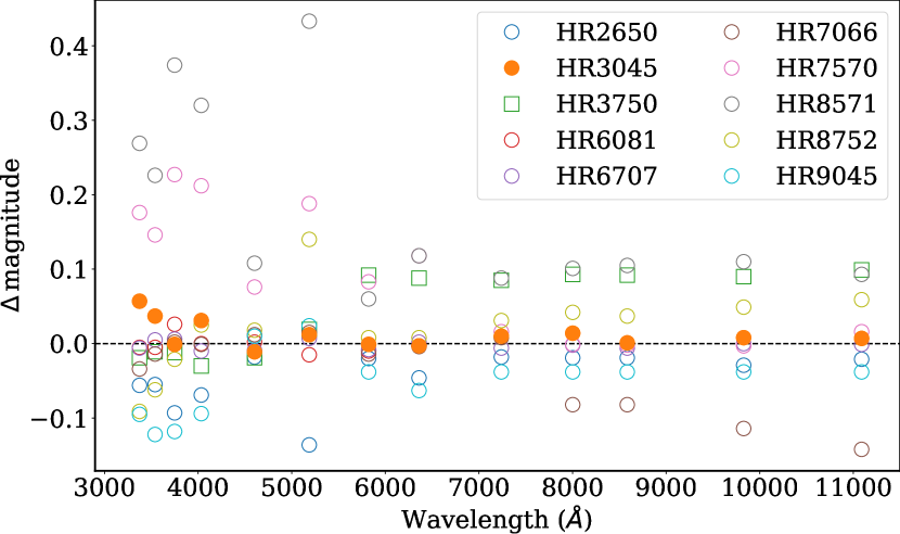
Figure 4: Differences in the photometric measurements of 1 star from S76 (HR3750, open square) and 9 stars from BAS97 (the remaining objects) in common with the JM75 sample. Open circles indicate variable stars. HR3750 is a binary system. The r.m.s. for HR3045, the only non-variable and non-binary star, is $0.018$ mag.

The comparison of the common stars in the three original sources is shown in Fig. 4. Even though most of these repeated stars are variable, the scatter of the photometric measurements (except for the bluest filters) is compatible with a $~{}\sim 0.1$ mag dispersion. Focusing on HR3045, the only star that is not variable and that does not belong to a binary system, the r.m.s. for the 13 photometric measurements is 0.018 mag, which is perfectly compatible with the probable errors of single observations in JM75 and S76, reported by Schuster (1982b, see his Table 2) to be $\sim 0.02$ mag. The photometric measurements for these 10 repeated stars have been averaged for the subsequent work.

4 Spectrum fitting

Table 2: First 10 rows of the table with the final sample, constituted by 1346 stars, comprising the UCM library of spectrophotometric standards. The full table is electronically available at %****␣paper_RGB.tex␣Line␣525␣****http://guaix.ucm.es/rgbphot. Column description: (1) HR number; (2)–(3) star coordinates (J2000), as provided by Simbad; (4) identificacion of the companion star for double star systems (see Table 3); (5) additional name when the star is a known variable according to Simbad; (6) variability type from Samus’ et al. (2017), as provided by Simbad; (7)–(19) absolute flux densities in each of the C13 photometric bandpasses (in units of erg s^-1 cm^-2 Å^-1); (20)–(22) effective temperature, surface gravity and metallicity derived from the best CK04 fit to the available photometric data, with the corresponding uncertainties derived from the bootstrapped spectra (note that the quoted uncertainties are simply lower limits to the expected random errors in the stellar atmospheric parameters; see discussion in Sect. 4.2); (23) scaling factor to convert the fitted CK04 model fluxes into absolute flux densities using Eq. (9); (24)–(25) Johnson $B$ and $V$ magnitudes (VEGA system), extracted from Simbad; (26)–(27) synthetic Johnson $B$ and $V$ magnitudes (VEGA system), measured in the best CK04 fit, with their corresponding uncertainties estimated from the bootstrapped spectra; (28)–(30) synthetic RGB magnitudes (AB system), measured in the best CK04 fit, using the bandpass definitions given in Table 5, with uncertainties estimated from bootstrapping.

(1)	(2)	(3)	(4)	(5)	(6)	(7)	(8)	(9)	(10)
HR	RA (°)	DEC (°)	Double	Variable	Var.Type	$f_{33}^{\star}$ ($\times 10^{-9}$)	$f_{35}^{\star}$ ($\times 10^{-9}$)	$f_{37}^{\star}$ ($\times 10^{-9}$)	$f_{40}^{\star}$ ($\times 10^{-9}$)
0003	1.3339247	$-$5.7076189	—	BC Psc	RS	0.008065	0.009427	0.011144	0.024608
0005	1.5658922	58.4367280	—	V640 Cas	CST:	0.006548	0.006900	0.007224	0.012313
0015	2.0969161	29.0904311	—	alf And	ACV:	1.034568	0.962187	0.997723	1.354483
0021	2.2945217	59.1497811	—	bet Cas	DSCTC	0.272195	0.284138	0.377964	0.622496
0025	2.3526731	$-$45.7474253	—	—	—	0.015074	0.019376	0.021859	0.051003
0027	2.5801942	46.0722722	—	—	—	0.014914	0.016286	0.027913	0.046962
0033	2.8160733	$-$15.4679794	—	—	—	0.027421	0.028911	0.031828	0.046545
0039	3.3089633	15.1835936	—	gam Peg	BCEP	0.956366	0.839646	0.742393	0.785749
0045	3.6506856	20.2067003	—	NSV 99	undef	0.001080	0.001705	0.002336	0.007366
0048	3.6600689	$-$18.9328653	—	AE Cet	LB:	0.001156	0.001833	0.002564	0.008143

(1)	(11)	(12)	(13)	(14)	(15)	(16)	(17)	(18)	(19)
HR	$f_{45}^{\star}$ ($\times 10^{-9}$)	$f_{52}^{\star}$ ($\times 10^{-9}$)	$f_{58}^{\star}$ ($\times 10^{-9}$)	$f_{63}^{\star}$ ($\times 10^{-9}$)	$f_{72}^{\star}$ ($\times 10^{-9}$)	$f_{80}^{\star}$ ($\times 10^{-9}$)	$f_{86}^{\star}$ ($\times 10^{-9}$)	$f_{99}^{\star}$ ($\times 10^{-9}$)	$f_{110}^{\star}$ ($\times 10^{-9}$)
0003	0.045110	0.048056	0.055965	0.055715	0.047546	0.042668	0.039957	0.034183	0.026974
0005	0.015360	0.014287	0.014343	0.013207	0.010510	0.008935	0.007667	0.006164	0.004537
0015	0.949220	0.642224	0.456478	0.335422	0.225124	0.161805	0.127347	0.090751	0.061170
0021	0.589519	0.485483	0.416094	0.351972	0.266133	0.212027	0.175507	0.135903	0.098852
0025	0.086732	0.095887	0.110133	0.104018	0.087565	0.078870	0.073035	0.061796	0.052358
0027	0.044648	0.038470	0.034585	0.029620	0.023448	0.019148	0.016498	0.013264	0.010151
0033	0.047392	0.042263	0.038594	0.033799	0.027282	0.022794	0.019054	0.014683	0.011011
0039	0.494316	0.326709	0.220809	0.159055	0.101730	0.069933	0.053288	0.035159	0.023059
0045	0.026858	0.035779	0.051488	0.062204	0.079683	0.091648	0.090080	0.092416	0.082166
0048	0.032928	0.047326	0.070281	0.085556	0.108490	0.123857	0.123218	0.124770	0.105232

(1)	(20)		(21)		(22)		(23)
HR	$T_{\rm eff}$ (K)		$\log g$		[M/H]		$c_{\rm sc}$ ($\times 10^{-17}$)
0003	4732$\;\pm\;$	21	3.088$\;\pm\;$	0.320	0.000$\;\pm\;$	0.072	1.8003
0005	5762$\;\pm\;$	50	4.809$\;\pm\;$	0.291	0.200$\;\pm\;$	0.095	0.1705
0015	12827$\;\pm\;$	101	4.484$\;\pm\;$	0.116	0.500$\;\pm\;$	0.000	0.5109
0021	6917$\;\pm\;$	81	3.229$\;\pm\;$	0.099	$-$0.085$\;\pm\;$	0.153	2.3213
0025	4824$\;\pm\;$	29	2.522$\;\pm\;$	0.312	0.000$\;\pm\;$	0.043	3.0634
0027	6181$\;\pm\;$	31	1.299$\;\pm\;$	0.107	$-$0.801$\;\pm\;$	0.158	0.3045
0033	6217$\;\pm\;$	76	3.912$\;\pm\;$	0.211	$-$0.386$\;\pm\;$	0.126	0.3484
0039	21414$\;\pm\;$	393	4.192$\;\pm\;$	0.330	$-$2.000$\;\pm\;$	0.000	0.1248
0045	3748$\;\pm\;$	16	1.202$\;\pm\;$	0.070	0.429$\;\pm\;$	0.080	11.7681
0048	3750$\;\pm\;$	3	0.770$\;\pm\;$	0.117	0.500$\;\pm\;$	0.010	15.6778

(1)	(24)	(25)	(26)		(27)		(28)		(29)		(30)
HR	Johnson $B_{\rm Simbad}$	Johnson $V_{\rm Simbad}$	Johnson $B_{\rm CK04}$		Johnson $V_{\rm CK04}$		standard $B$		standard $G$		standard $R$
0003	5.65	4.61	5.649 $\;\pm$	0.011	4.583 $\;\pm$	0.010	5.128 $\;\pm\;$	0.010	4.680 $\;\pm\;$	0.010	4.357 $\;\pm\;$	0.008
0005	—	—	6.691 $\;\pm$	0.013	5.985 $\;\pm$	0.009	6.307 $\;\pm\;$	0.012	6.044 $\;\pm\;$	0.009	5.862 $\;\pm\;$	0.009
0015	1.95	2.06	1.914 $\;\pm$	0.010	2.021 $\;\pm$	0.011	1.834 $\;\pm\;$	0.010	1.983 $\;\pm\;$	0.011	2.144 $\;\pm\;$	0.012
0021	2.61	2.27	2.580 $\;\pm$	0.015	2.248 $\;\pm$	0.010	2.347 $\;\pm\;$	0.014	2.268 $\;\pm\;$	0.011	2.234 $\;\pm\;$	0.008
0025	4.89	3.87	4.916 $\;\pm$	0.011	3.863 $\;\pm$	0.008	4.399 $\;\pm\;$	0.010	3.958 $\;\pm\;$	0.009	3.653 $\;\pm\;$	0.008
0027	5.44	5.04	5.386 $\;\pm$	0.012	4.978 $\;\pm$	0.009	5.133 $\;\pm\;$	0.013	5.009 $\;\pm\;$	0.010	4.932 $\;\pm\;$	0.008
0033	5.38	4.89	5.358 $\;\pm$	0.012	4.865 $\;\pm$	0.008	5.075 $\;\pm\;$	0.012	4.906 $\;\pm\;$	0.009	4.797 $\;\pm\;$	0.007
0039	2.61	2.84	2.568 $\;\pm$	0.010	2.770 $\;\pm$	0.013	2.529 $\;\pm\;$	0.011	2.719 $\;\pm\;$	0.013	2.917 $\;\pm\;$	0.013
0045	6.38	4.80	6.342 $\;\pm$	0.015	4.714 $\;\pm$	0.010	5.668 $\;\pm\;$	0.014	4.879 $\;\pm\;$	0.010	4.326 $\;\pm\;$	0.014
0048	6.12	4.46	6.101 $\;\pm$	0.015	4.383 $\;\pm$	0.009	5.389 $\;\pm\;$	0.009	4.554 $\;\pm\;$	0.009	3.981 $\;\pm\;$	0.012

4.1 The fitting procedure

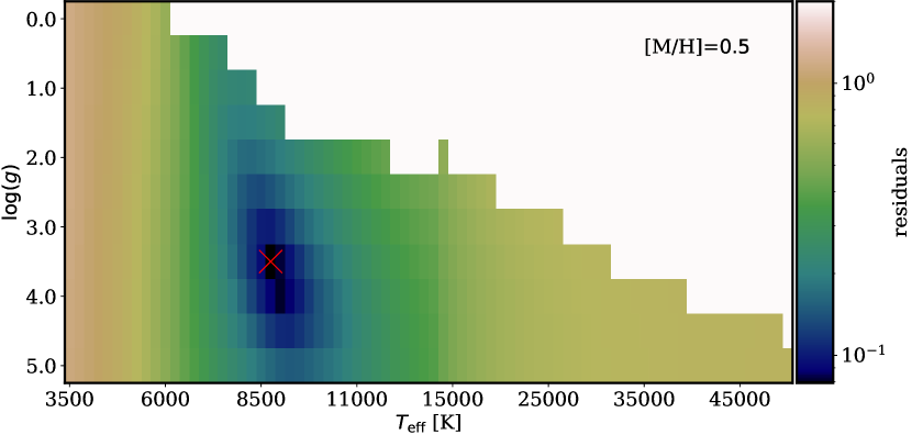
Figure 5: Example of computation of initial atmospheric stellar parameters in the fit of the C13 photometric data of the star HR7254 to the CK04 models. Each plot shows the residuals obtained after determining the best scaling factor when fitting the modeled spectra with different $T_{\rm eff}$ and $\log g$ values at a fixed metallicity ([M/H], given in the upper right corner). The residuals were computed as $\sqrt{\chi^{2}/N_{\rm bands}}$, with $\chi^{2}$ given by Eq. (6). The white areas indicate the stellar parameter space not available in the models. The red cross in each panel marks a local minimum, i.e., the $T_{\rm eff}$ and $\log g$ values that provide the best fit at the considered [M/H]. A large red filled circle has been overplotted in the panel where the global minimum is reached.

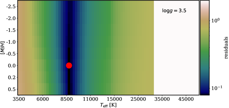
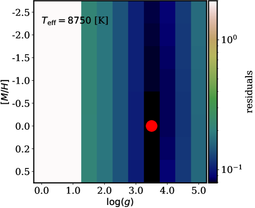
Figure 6: Residuals of the same fit displayed in Fig. 5, corresponding to the star HR7254. These two panels show two perpendicular views in the 3D parameter space around the global minimum found at $T_{\rm eff}=8750$ K, ${\rm[M/H]}=0.0$ and $\log g=3.5$ in the first step of the fitting procedure discussed in Sect. 4.1.

The first step before attempting to estimate the synthetic RGB photometry of the bright star sample was the fit of the spectral energy distribution of each star to the stellar model spectrum that best matched the available 13C photometric data. For that purpose, we have chosen the Stellar Atmosphere Models by Castelli & Kurucz (2003, hereafter CK04), as provided by the STScI web page. An important advantage of these models is that they can be easily interpolated using the Python package stsynphot (Lim, 2018, available online) for any arbitrary $T_{\rm eff}$, [M/H] and $\log g$ selection (within the parameter space covered by the models). Since the bright star sample is constituted by nearby objects, it is safe to assume that most of them will not be strongly affected by interstellar reddening. For that reason, we have not included any correction for this effect in the subsequent fits. In any case, here we are aiming at providing accurate photometry of the observed (i.e., uncorrected) RGB fluxes, and the fact of excluding this type of correction will only translate in a systematic deviation of the derived stellar parameters.

It is important to highlight that it is not the aim of this work to determine accurate stellar atmospheric parameters for each star, but to obtain a good fit to the available 13C photometric data in order to derive reliable spectral energy distributions that facilitate the proper computation of synthetic RGB magnitudes. The comparison with observed spectra, shown in section 4.4, indicates that this is actually the case.

The initial 13C stellar magnitudes were converted into absolute flux densities (erg s^-1 cm^-2 Å^-1) using the conversion given by JM75 (the Fortran IV code provided in their Table 5 was transformed to Python to facilitate this task). The selection of the best CK04 model for each star was accomplished in two steps:

1. Initial determination of the atmospheric stellar parameters using all the available CK04 models at their pre-computed sampling grid in the parameter space. In particular, the CK04 atlas provides models for abundances [M/H]=$-2.5$, $-2.0$, $-1.5$, $-1.0$, $-0.5$, $0.0$, $+0.2$ and $+0.5$, with effective temperatures ranging from 3500 to 50000 K, and $\log g$ (surface stellar gravity, with  $g$  in cm s^-2) from 0.0 to 5.0 dex. A simple chi-square minimization process was performed, by adjusting the arbitrary constant $c_{\rm sc}$ necessary to scale each model prediction to the absolute C13 flux densities. For this purpose, the stellar fluxes for the star $f^{\star}_{i}$ and the model $f^{\rm CK04}_{i}$ in each of the $N_{\rm bands}$ photometric bandpasses were normalized by their mean values

   $$f^{\star}_{{\rm nor},i} =\frac{f^{\star}_{i}}{\langle f^{\star}\rangle}, \;\;{\rm with} \langle f^{\star}\rangle =\frac{1}{N_{\rm bands}}\sum_{i=1}^{N_{\rm bands}}f^{\star}_{i},$$ (4)

   $$f^{\rm CK04}_{{\rm nor},i} =\frac{f^{\rm CK04}_{i}}{\langle f^{\rm CK04}\rangle}, \;\;{\rm with} \langle f^{\rm CK04}\rangle =\frac{1}{N_{\rm bands}}\sum_{i=1}^{N_{\rm bands}}f^{\rm CK04}_{i}.$$ (5)

   The initial stellar fluxes  $f_{i}^{\star}$  (with  $i=33,\,35,\ldots,110$ indicating the 13C photometric band), computed from the published photometric data, are listed in Table 2, columns (5)–(17).

   An objective function to be minimized was defined at this point as

   $$\chi^{2}(c_{\rm nor})=\sum_{i=1}^{N_{\rm bands}}\left(f^{\star}_{{\rm nor},i}-c_{\rm nor}f^{\rm CK04}_{{\rm nor},i}\right)^{2},$$ (6)

   where $c_{\rm nor}$ is an intermediate scaling factor between the normalized stellar and model fluxes. By equating to zero the first derivative of the last equation, it is immediate to obtain

   $$c_{\rm nor}=\frac{\sum_{i=1}^{N_{\rm bands}}f^{\star}_{{\rm nor},i}\,f^{\rm CK04}_{{\rm nor},i}}{\sum_{i=1}^{N_{\rm bands}}\left(f^{\rm CK04}_{{\rm nor},i}\right)^{2}}.$$ (7)

   Finally, the sought scaling factor $c_{\rm sc}$ is computed as

   $$c_{\rm sc}=c_{\rm nor}\frac{\langle f^{\star}\rangle}{\langle f^{\rm CK04}\rangle},$$ (8)

   which allows to convert the CK04 model fluxes into absolute flux densities as

   $$f^{\star}=c_{\rm sc}f^{\rm CK04}.$$ (9)

   At this stage, the whole parameter space was sampled using all the initially available combinations of the three stellar parameters. The global minimum of the objective function in this comprehensive search led to an initial guess for $T_{\rm eff}$, [M/H], and $\log g$, which were refined in the subsequent step. A graphical example of this initial computation is shown in Figs. 5 and 6. The comparison of these plots indicates that, not surprisingly, $T_{\rm eff}$ is the main parameter governing the variation of the $\chi^{2}$ value, followed by $\log g$. These two parameters are correlated, as shown by the oblique orientation of the minimum valley in Fig. 5. In addition, the role of [M/H] is quite small, as revealed by the almost undetectable variation of the residuals with this parameter in Fig. 6. This result gives support to the idea that the derived stellar parameters should not be considered as extremely accurate.

2. Refinement of the atmospheric stellar parameters: the initial $T_{\rm eff}$, [M/H], and $\log g$ values were employed as the starting point in the parameter space to compute a more refined solution. For that purpose, we used a numerical minimization process based on the Nelder-Mead method (Nelder & Mead, 1965) with the help of the Python package lmfit (Newville et al., 2014, available online). During this process, the CK04 model predictions were interpolated at arbitrary locations within the valid stellar atmospheric parameter space, as required by the objective function to be minimized. The use of a good starting point, obtained in the previous step, facilitated the convergence of this process. The final $T_{\rm eff}$, [M/H] and $\log g$ parameters for each star are given in Table 2, columns (18)–(20).

   4.2 Uncertainties in the fitting procedure

   

   

   

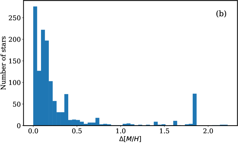
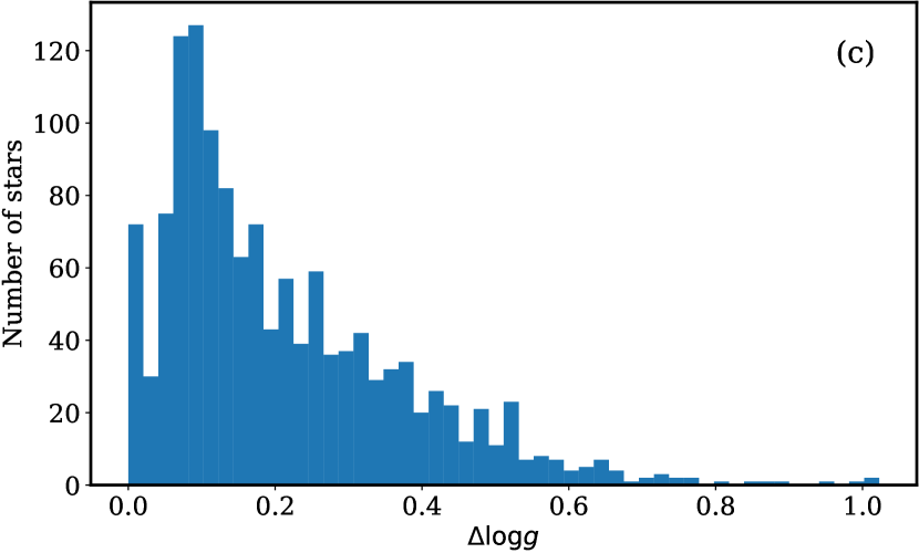
   Figure 7: Distribution of random uncertainties in the derived stellar atmospheric parameters in the final sample of fitted CK04 models, estimated from the bootstrapping method described in Sect. 4.2. Panel (a): relative errors in effective temperature. Panels (b) and (c): absolute errors in metallicity and surface gravity. It is important to highlight that these uncertainties are simply lower limits to the expected random errors in the stellar atmospheric parameters, as explained in the text.

   Two main sources of uncertainties have been considered: i) systematic errors due to the inability of the adopted CK04 models to properly reproduce the spectral energy distribution of the stars, and ii) random errors in the fitted C13 photometric data.

   Since there is not an easy way to fix model fits exhibiting C13 residuals with a systematic variation as a function of wavelength, we decided to get rid of those stars with unreliable fits, following the criteria described in Sect. 4.3.

   On the other hand, the impact of random errors in the fitting process has been determined by generating bootstrapped absolute flux densities, using for that purpose the already mentioned probable error of 0.02 mag in the C13 photometric data, and repeating the whole fitting procedure in each simulated set of C13 photometric data for every star. This allowed obtaining an initial estimate of the uncertainties in the fitted stellar parameters, which are given in the corresponding columns (18)–(20) of Table 2, and graphically displayed in Fig. 7. It is important to stress that these random uncertainties must not be understood as the actual uncertainties associated to the derived atmospheric stellar parameters. As previously mentioned, no attempt to introduce an interstellar reddening correction has been performed. Furthermore, we are constrained to the capability of CK04 models to provide an accurate modelling of actual stellar spectra, without considering, for example, the impact of the assumed line opacities and chemical abundances, to mention some of the additional relevant parameters that should be considered to obtain reliable physical descriptions of the stellar atmospheres. Once the CK04 set of stellar atmosphere models has been adopted, the quoted random errors are just a lower limit to the actual $T_{\rm eff}$, [M/H] and $\log g$ uncertainties for each star. Nevertheless, the quoted values can be compared with the sampling of the atmospheric parameters at which the CK04 models are provided. In particular, the effective temperature is sampled with $\Delta T_{\rm eff}/T_{\rm eff}$ ranging from 0.02 (hot stars) to 0.07 (cool stars), whereas gravity and metallicity are sampled at $\Delta(\log g)=0.5$, and $\Delta{\rm[M/H]}$ ranging from 0.2 to 0.5, respectively. Comparing these numbers with the distributions displayed in Fig. 7, it is clear that in most cases the derived uncertainties are within the considered sampling steps, which indicates that, at least from the point of view of the fitting procedure, each one of the CK04 models is different enough from its neighbouring models within the 3D parameter space even after bootstrapping the C13 photometric data. This reinforces the usefulness of Step 2 (see Sect. 4.1) devoted to the refinement of the atmospheric stellar parameters. In addition, the bootstrapping method provided a collection of bootstrapped fitted spectra associated to every single star, that were employed later to estimate random uncertainties in the synthetic photometry performed on the CK04 model fits.

   It is important to highlight that although the numerical minimization procedure adopted for this work is robust, the computation time spent on each individual fit is not negligible. In particular, the adopted Nelder-Mead method required the evaluation of the objective function in many points (typically a few hundreds) within the 3D parameter space defined by $T_{\rm eff}$, $\log g$ and [M/H], which in turn translated into the corresponding number of interpolations of the CK04 models. The median computation time for every fit amounted to a few minutes. For that reason, we decided to generate a number of bootstrapped spectra not excessively large, in order to apply this technique to the whole final sample and not only to a representative subsample of stars. Finally, this total number of bootstrapped spectra for each individual star was set to 30, which leads to uncertainties in the uncertainties of $\sim 13$%.

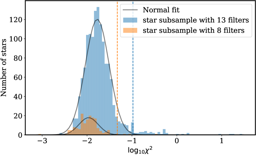
Figure 8: Histogram of minimum values of the objective function obtained during the fitting procedure of CK04 models. The initial sample (1522 stars) were segregated according to the number of available photometric bandpasses (13 or 8). The black lines indicate the robust fit to Normal distributions. The vertical dashed lines mark the 3$\sigma$ location above the median value, which corresponds to $\chi^{2}_{3\sigma}\simeq 0.105$ for the 1359 stars observed with 13 filters, and $\chi^{2}_{3\sigma}\simeq 0.047$ for the 163 stars observed with 8 filters.

4.3 Cleaning the sample

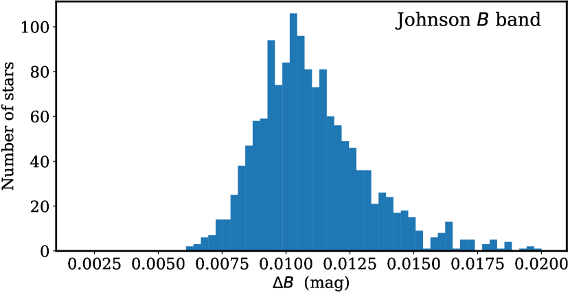
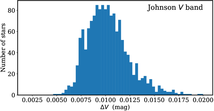
Figure 9: Distribution of random uncertainties in the synthetic Johnson $B$ and $V$ measurements performed on the final sample of fitted CK04 models, estimated from the bootstrapping method described in Sec. 4.2. The median values are $\Delta B=0.011$ mag (top panel) and $\Delta V=0.010$ mag (bottom panel).

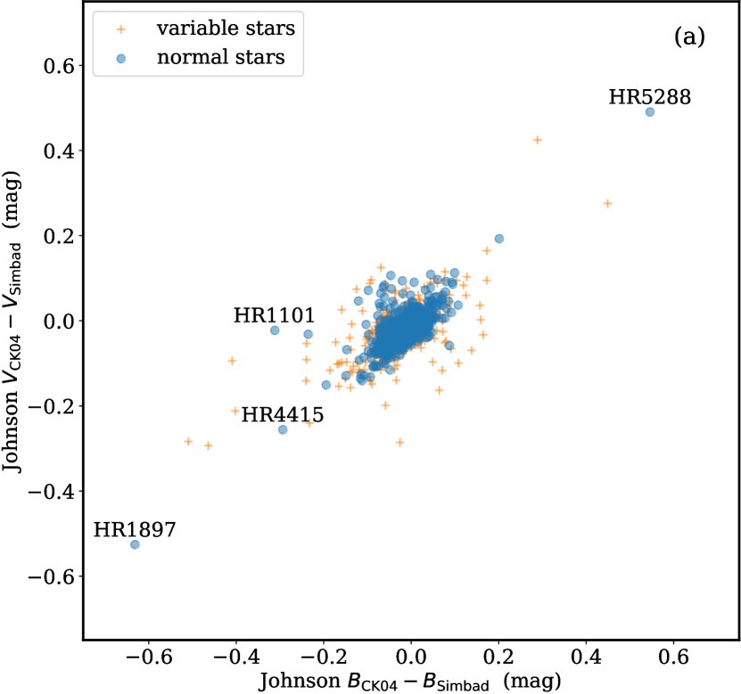
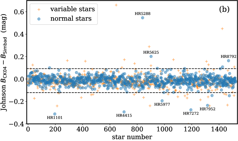
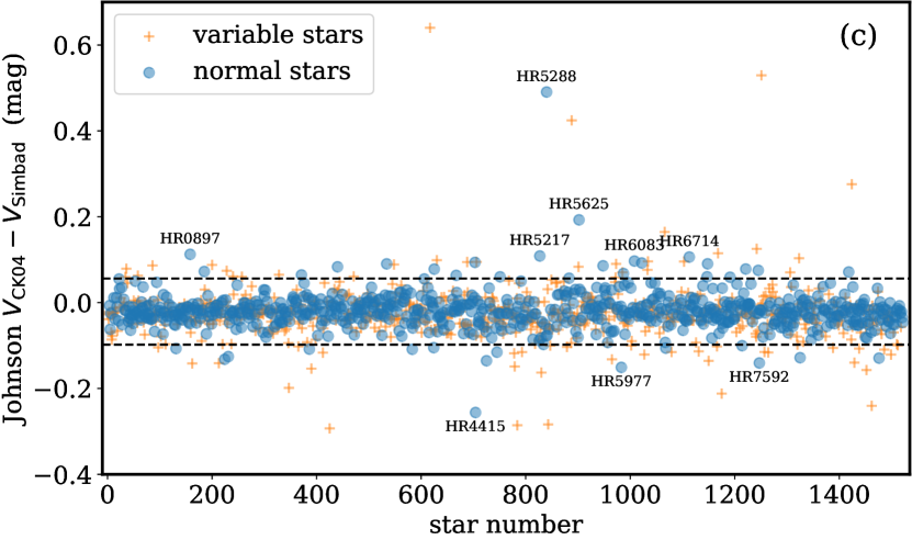
Figure 10: Differences between the synthetic Johnson $B$ and $V$ magnitudes computed using the CK04 model fits and the tabulated $B$ and $V$ data available in Simbad. Known variable stars (according to Simbad) are plotted with orange crosses, whereas normal stars (i.e., non-variable) are represented with blue filled circles. Panel (a) shows that, not surprisingly, the errors in $B$ and $V$ are correlated. The individual analysis of the differences within each photometric band are shown in panels (b) and (c). The dashed lines in the last two panels correspond to the robust $\pm 3\sigma$ region around the median. A few stars, exhibiting large deviations, are labelled in each panel.

Table 3: Double stars from the JM75 sample for which the individual fluxes of the two stars have been coadded to derive the resulting integrated $B$ and $V$ magnitudes (last two columns). Star#1 is the initial star identification provided in JM75. Star#2 is the companion star (in some cases the companion star is brighter than Star#1). For some stars the magnitude in one of the two filters is missing. The quoted $B$ and $V$ magnitudes for the individual stars, as well as the spectral type, correspond to the data retrieved from the Simbad database. Stars marked with an asterisk in the first column were finally removed from the final sample due to large discrepancies between the Simbad data and the predicted $B$ and $V$ magnitudes, as explained in Sect. 4.3. The fourth column in Table 2 provides the name of the companion star for the double star systems incorporated in the final stellar sample.

Star#1					Star#2					Star#1+#2
Name	$B_{1}$	$V_{1}$	SpT1	X	Name	$B_{2}$	$V_{2}$	SpT2	X	$B_{1+2}$	$V_{1+2}$
HR0545	4.558	4.589	A0V		HR0546	4.490	4.520	A2IV		3.771	3.801
∗HR0897	3.330	3.180	A3IV–V		HR0898	4.200	4.110	A1V		2.928	2.796
HR1211	6.190	6.090	A1V		HR1212	5.590	4.700	G6.5III		5.096	4.434
∗HR1897	6.300	6.390	O9.5IV		$\theta^{2}$ Ori B	6.290	6.380	B2–B5		5.542	5.632
∗HR1948	1.790	1.880	O9.2Ib		HR1949	3.550	3.730	O9.5II–III		1.594	1.698
HR2298	4.583	4.398	A8V		HR2299	6.990	6.600	F5V		4.471	4.264
HR2735	6.046	5.623	F0/3		HR2736	4.774	3.746	K0III		4.481	3.569
HR2890	—	3.000	A0–A2		HR2891	—	1.900	A1.5IV		—	1.564
HR3890	3.250	2.990	A9		HR3891	6.080	5.990	B7III		3.173	2.924
∗HR3925	5.680	5.810	B5V		HD85980B	8.260	8.230	—		5.584	5.699
∗HR4057	3.130	—	K1III		HR4058	3.400	—	G7III		2.504	—
HR4374	5.410	4.770	G2V		HR4375	4.790	4.250	F8.5V		4.304	3.727
∗HR4730	1.100	1.280	B0.5IV		HR4731	1.410	1.580	B1V		0.491	0.667
HR4825	3.800	3.440	F1–F2V		HR4826	3.850	3.490	F0–F2V		3.072	2.712
HR5054	2.271	2.220	A1.5V		HR5055	4.050	3.880	A1–A7IV–V		2.078	2.007
HR5328	7.080	6.690	F2V		HR5329	4.740	4.510	A7IV		4.621	4.373
HR5459	0.720	0.010	G2V		HR5460	2.210	1.330	K1V		0.475	$-$0.272
HR5475	4.792	4.893	B9III		HR5476	5.979	5.761	A6V		4.478	4.490
HR5477	4.590	4.510	—		HR5478	4.560	4.510	—		3.822	3.757
HR5505	4.853	4.801	A0V		HR5506	3.610	2.450	K0II–III		3.310	2.332
HR5788	5.380	5.130	F0IV		HR5789	4.390	4.140	F0IV		4.023	3.773
∗HR5977	5.350	4.870	F5V		HR5978	5.640	5.160	F4(V)		4.733	4.253
∗HR5984	2.550	2.620	B1V		HR5985	4.870	4.890	B2V		2.429	2.493
∗HR6406	4.670	3.330	M5Ib–II		HR6407	6.030	5.322	G5III+F2V		4.397	3.169
HR6484	5.395	5.398	A0V		HR6485	4.476	5.510	B9.5III		4.088	4.113
HR6896	6.320	4.860	K1/2III		21 Sgr B	7.680	7.390	—		6.047	4.759
HR7293	7.400	—	G3V		HR7294	7.220	—	G2V		6.554	—
HR7921	6.672	5.638	G8IIb		49 Cyg B	8.150	8.090	B9.9		6.424	5.530
HR7947	5.530	4.960	F8V		HR7948	5.260	4.250	K1IV		4.634	3.795
∗HR8148	7.500	6.680	G7V		HD202940B	10.980	9.960	K5		7.457	6.609
HR8309	5.140	4.700	F7V		HR8310	6.670	6.120	F3V		4.903	4.440
HR8545	6.830	6.220	G2V		53 Aqr B	6.960	6.320	G3V		6.140	5.516
HR8558	4.890	4.490	F2IV/V		HR8559	4.790	4.340	F2IV/V		4.086	3.660
HR9074	6.910	6.400	F8		BD+32 4747B	7.210	6.660	G1		6.297	5.770

Table 4: References for the $B$ and $V$ photometric data extracted from the Simbad database and employed for the comparison with the synthetic magnitudes computed in the fitted CK04 models. (1) ADS bibcode, (2) number of stars with $B$ photometry, (3) number of stars with $V$ photometry, and (4) reference.

Bibcode	$B$	$V$	Reference
1965LowOB...6..167A	1	1	Alcaino (1965)
1966CoLPL...4...99J	4	4	Johnson et al. (1966)
1967ArA.....4..375L	2	2	Lodén (1967)
1968ArA.....4..425L	1	1	Lodén (1968)
1969ArA.....5..149L	1	1	Lodén (1969a)
1969ArA.....5..161L	2	2	Lodén (1969b)
1969ArA.....5..231L	1	1	Lodén & Nordström (1969)
1978A&AS...34....1N	3	3	Nicolet (1978)
1982A&AS...47..221R	2	1	Rakos et al. (1982)
1985A&AS...61..331O	2	2	Oja (1985)
1991A&AS...89..415O	10	7	Oja (1991)
1993A&AS..100..591O	52	51	Oja (1993)
1997JApA...18..161Y	5	6	Yoss & Griffin (1997)
2000A&A...355L..27H	391	390	Høg et al. (2000)
2001AJ....122.3466M	0	1	Mason et al. (2001)
2002A&A...384..180F	37	39	Fabricius et al. (2002)
2002yCat.2237....0D	788	765	Ducati (2002)
2006AJ....132..111J	6	6	Joner et al. (2006)
2009ApJ...694.1085V	0	17	van Belle & von Braun (2009)
2011A&A...531A..92R	7	7	Röser et al. (2011)
2012yCat.1322....0Z	4	4	Zacharias et al. (2012)
2013ApJ...764..114H	1	1	Hsu et al. (2013)
2014ApJ...794...36H	1	1	Hernández et al. (2014)

After applying the previously described fitting method to the initial sample of 1522 stars, we discovered that some of the CK04 model fits were not reliable. After sorting the stars by the minimum value of the objective function obtained at the end of the minimization process, we visually examined all the individual fits to establish potential biases in the fitting procedure. At this point the following criteria were sequentially employed to remove stars from the initial sample:

1. Stars with large objective function values in the minimization process: we analysed the histograms of the resulting $\chi^{2}$ (Fig. 8), segregating the sample in two groups, depending on the number of photometric bands available for each star (13 and 8 bands for 1359 and 163 stars, respectively). In both cases, although the distributions are roughly normal, there is a tail of stars with large $\chi^{2}$ values. The $3\sigma$ cut (shown as the dotted vertical lines) is $\chi^{2}_{3\sigma}\simeq 0.105$ and $0.047$, for the subsamples with 13 and 8 bands, respectively. We decided to remove the 48 stars with $\chi^{2}$ above these threshold values. Among them, 43 stars are known variables according to Simbad or exhibit emission lines (not considered in our fitting procedure), and 5 show large red or blue fluxes that could not be properly fitted with the CK04 models.

2. Stars with large discrepancies in synthetic Johnson $B$ and $V$ magnitudes when compared with the available data in the Simbad database. These magnitudes were computed in the VEGA system, using as reference the flux density (factor $f_{r}(\lambda)$ in Eq. 3) of the Vega spectrum alpha_lyr_stys_010.fits, available at the CALSPEC database (Bohlin et al., 2014). In addition, the spectral sensitivity curves for the $B$ and $V$ filters from Bessell & Murphy (2012, see their Table 1) were employed. We have chosen these two classical bandpasses because their wavelength coverage overlaps with that of typical RGB Bayer-like photometric systems. The expected random errors in these synthetic measurements, estimated from the bootstrapping strategy described in Sect. 4.2 and displayed in Fig. 9, are small: $\Delta B\sim 0.011$ mag and $\Delta V\sim 0.010$ mag. Since some stars in the original JM75 sample were flagged as double (i.e., more than one star were observed simultaneously), the corresponding flux coaddition was performed to compute the expected $B$ and $V$ magnitudes in those cases (see Table 3; the name of the companion stars are also provided in the fourth column of Table 2). Interestingly, the spectra of these double stars did not lead to large $\chi^{2}$ values in Fig. 8, mainly because the light of the combined spectrum was dominated by the brightest star in the system or because in several cases the difference in spectral type was not large. The comparison between the synthetic and the tabulated Simbad magnitudes is shown in Fig. 10. It is important to highlight that the Simbad measurements come from a relatively high number of different sources (see Table 4). Thus, it is expected that the compiled data are heterogeneous in photometric quality and not completely free from systematic offsets. This problem, together with additional sources of systematic errors, such as the inability of the adopted CK04 model fitting procedure to reproduce the actual star spectra in all cases, the presence of unaccounted stellar variability, and the inherent photometric uncertainties within the C13 photometric data themselves, make the correlation exhibited by the magnitude differences in Fig. 10(a) not unexpected. In any case, an independent analysis of $B_{\rm CK04}\!-\!B_{\rm Simbad}$ and $V_{\rm CK04}\!-\!V_{\rm Simbad}$ has been performed, as displayed in Figs. 10(b) and (c). We decided to follow a statistical approach to remove from the star sample those objects with large deviations in either $B$ or $V$. For that purpose, we first computed the median values ($-0.014$ mag and $-0.021$ mag for $B_{\rm CK04}\!-\!B_{\rm Simbad}$ and $V_{\rm CK04}\!-\!V_{\rm Simbad}$, respectively) and rejected those stars outside the robust $\pm 3\sigma$ interval around the median value ($\pm 0.107$ mag and $\pm 0.077$ mag). A total of 128 stars were removed from the sample, being $\sim 2/3$ of this rejected subsample (82 stars) constituted by known variables.

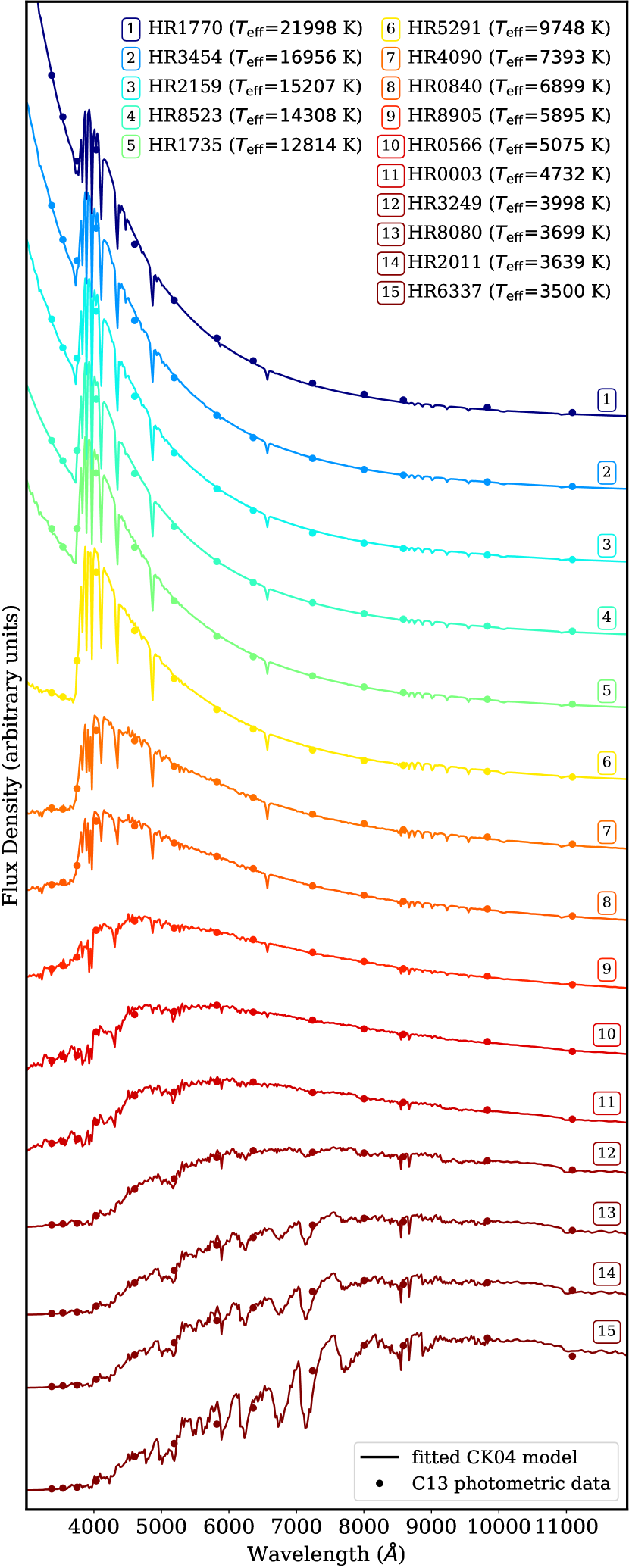
Figure 11: Examples of spectrum fits to stars with different effective temperature. The filled circles correspond to the C13 photometric data (flux densities in arbitrary units) from JM75. The continuous lines are the fitted CK04 models. The spectra have been numbered by decreasing fitted $T_{\rm eff}$ (from Table 2), and their identifications are given in the upper key.

After this cleaning process, the final sample of fitted CK04 models is formed by 1346 stars, that constitute the UCM (Universidad Complutense de Madrid) library of spectrophotometric standards. Although an important fraction of them ($\sim 44$%, 594 stars) are still classified as known variables, we have decided to keep these objects in the final list since no significant differences with the Simbad tabulated measurements have been found. Some of these variables are eclipsing binaries, and most of the time they constitute suitable reference stars. In any case, columns (5) and (6) in Table 2 provide an additional name and the corresponding classification (according to Samus’ et al., 2017) for the variable stars, and potential users of the derived RGB magnitudes should be well aware of this.

A selection of spectrum fits for stars exhibiting a wide range in effective temperature is shown in Fig. 11.

4.4 Comparison with Kiehling 1987

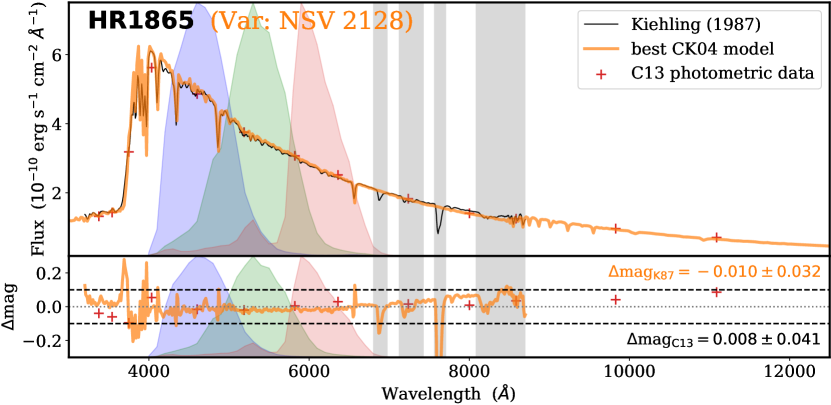
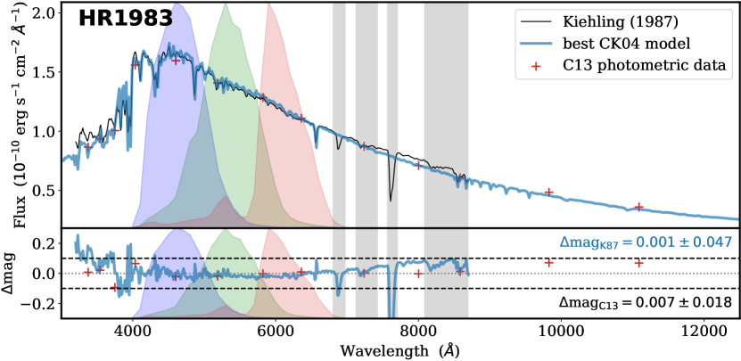
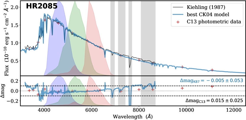
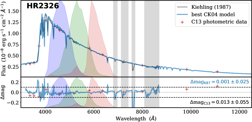
Figure 12: Comparison between the best CK04 fitted models and the spectrophotometric data from K87, for 4 stars (out of 39) in common with our final sample (all the plots corresponding to the 39 stars in common with K87 are provided in Appendix A). CK04 models are represented with thick blue lines for non-variable stars and thick orange lines for variable stars, while the K87 spectra are plotted with thin black lines. For each star, the upper panel displays the flux densities. The lower panel shows the corresponding residuals, in magnitudes, obtained when dividing the fluxes from CK04 models by the K87 measurements (continuous blue/orange line) or by the JM75 photometric data (red crosses); the dotted line marks the $\Delta$mag=0.0 level, whereas the dashed lines encompass the $\pm 0.1$ mag interval. For the variable stars one additional identification name is given in parenthesis. The C13 photometric data from JM75 are plotted with red crosses. The standard RGB spectral sensitivity curves, as defined in Section 5.1, are shown with blue, green, and red shaded areas, whereas the vertical grey bands correspond to the wavelength intervals where conspicuous telluric absorptions appear in the K87 spectra. See Sec. 4.4 for additional details.

To assess the quality of the fitting procedure just described, we have compared the compiled C13 photometric data and the fitted CK04 models with observed flux calibrated spectra. For that purpose, we have chosen the data from Kiehling (1987, hereafter K87), who published high-quality spectral energy distributions for 60 bright stars in the [3200–8600] Å wavelength interval, with typical internal flux errors of 0.02 mag (above 4000 Å) and 0.05 mag (below 4000 Å), when comparing observations from different nights. Fortunately, there were 39 stars in common between our final star sample and that from K87. Although 25 of them are known variable stars, according to Simbad, there is a very good agreement between K87 with both the C13 color photometric data and the corresponding CK04 fitted models.

The graphical comparison is shown in Fig. 12 (extended by Fig. A1). The wavelength regions of strong O₂ and H₂O telluric absorptions (wavelength intervals [6850–6950] Å, [7150–7350] Å, [7550–7650] Å, and [8150–8350] Å) were not corrected in the K87 data, and have been marked with a grey background in the displayed plots. The C13 measurements are plotted with filled red circles. The best CK04 model fits to these data are shown with thick blue (for non-variable stars) or orange (for variable stars) lines. The K87 spectra are overplotted with thin black lines. It is very important to highlight that the K87 spectra displayed in this figure are not fits to the C13 data, but calibrated spectral energy distributions, independently calibrated from the JM75 data. The resolution of these spectra was slightly reduced using a Gaussian kernel of 600 km/s in order to match the spectral resolution exhibited by the CK04 models. The 39 stars are sorted by HR name, and for each one two panels are shown: the top plot represents the flux density (erg s^-1 cm^-2 Å^-1); the lower panel shows the corresponding residuals, in magnitudes, obtained when dividing the fluxes from CK04 models by the K87 measurements (continuous blue/orange line) or by the JM75 photometric data (filled red circles). The dotted horizontal line in the residuals panel sets the $\Delta{\rm mag}=0$ level, while the two dashed lines encompass the $\pm 0.1$ mag interval. For each star, the residuals panel also provides two residuals summaries: $\Delta{\rm mag}_{\rm K87}$, the median and robust standard deviation when dividing the best CK04 model by the corresponding K87 spectrum (avoiding the marked telluric absorption regions), and $\Delta{\rm mag}_{\rm C13}$, the median and robust standard deviation when computing the ratio between the synthetic C13 fluxes (computed with the best CK04 model and the transmission curves displayed in Fig. 1) and the C13 measurements compiled in this work. In this sense, $\Delta{\rm mag}_{\rm K87}$ provides an indication of how well the K87 spectra agree with the JM75 photometric measurements, while $\Delta{\rm mag}_{\rm C13}$ summarizes the quality of the CK04 model fit to the JM75 data. The scatter in both parameters is in most cases (for non-variable stars) below $\pm 0.05$ mag.

5 Synthetic RGB magnitudes

5.1 Definition of a camera-independent RGB standard system

Figure 13: Comparison of RGB spectral sensitivity curves: the thin lines correspond to the 28 cameras measured by Jiang et al. (2013): Canon 1DMarkIII, Canon 20D, Canon 300D, Canon 40D, Canon 500D, Canon 50D, Canon 5DMarkII, Canon 600D, Canon 60D, Hasselblad H2, Nikon D3X, Nikon D200, Nikon D3, Nikon D300s, Nikon D40, Nikon D50, Nikon D5100, Nikon D700, Nikon D80, Nikon D90, Nokia N900, Olympus E-PL2, Pentax K-5, Pentax Q, Point Grey Grasshopper 50S5C, Point Grey Grasshopper2 14S5C, Phase One, and SONY NEX-5N. Then median values at each sampled wavelength are plotted as the thick lines, and the corresponding values are listed in Table 5.

Table 5: Renormalized median spectral sensitivity curves computed from the empirical sensitivity curves corresponding to the 28 cameras measured by Jiang et al. (2013) and displayed in Fig. 13. Column description: (1) wavelength (in Å); and (2)–(4) spectral sensitivity at each considered wavelength, for the median B, G and R bandpasses, respectively. In order to constraint the curves at the borders of the initial 4000–7200 Å interval sampled by the Jiang et al. (2013) measurements, two additional rows have been introduced in the table, at 3990 and 7210 Å, forcing the curves to drop rapidly to zero at these wavelengths. The information in this table is electronically available at http://guaix.ucm.es/rgbphot.

(1)	(2)	(3)	(4)
$\lambda$ (Å)	standard $B$	standard $G$	standard $R$
3990	0.0000000	0.0000000	0.0000000
4000	0.0150428	0.0030840	0.0034970
4100	0.1039736	0.0113570	0.0103892
4200	0.4892935	0.0388725	0.0238270
4300	0.7202255	0.0575395	0.0277668
4400	0.8216436	0.0791910	0.0180056
4500	0.9308637	0.1006650	0.0180360
4600	1.0000000	0.1360232	0.0218683
4700	0.9802917	0.2571178	0.0299132
4800	0.9275882	0.3809050	0.0339620
4900	0.7807393	0.4251800	0.0401877
5000	0.6143757	0.6113000	0.0430846
5100	0.4338580	0.7933000	0.0625152
5200	0.2491595	0.9033850	0.1111756
5300	0.1594246	1.0000000	0.1419566
5400	0.0947855	0.9064100	0.0849897
5500	0.0567221	0.8807233	0.0478130
5600	0.0273214	0.7437300	0.0521587
5700	0.0166126	0.6428150	0.1533735
5800	0.0114100	0.4597650	0.6503433
5900	0.0084778	0.3175050	1.0000000
6000	0.0048916	0.1819950	0.9353758
6100	0.0034230	0.0897230	0.8337379
6200	0.0029658	0.0485390	0.6858826
6300	0.0032853	0.0316045	0.5929939
6400	0.0037959	0.0229870	0.4600072
6500	0.0051010	0.0167670	0.3717754
6600	0.0050765	0.0112830	0.2205769
6700	0.0032660	0.0088190	0.1200198
6800	0.0011294	0.0046771	0.0371512
6900	0.0005127	0.0016871	0.0126072
7000	0.0002948	0.0007490	0.0037169
7100	0.0001017	0.0003077	0.0012105
7200	0.0000616	0.0001488	0.0005449
7210	0.0000000	0.0000000	0.0000000

Since the spectral sensitivity curves of Bayer-like color filter systems vary between different camera models, we have decided to define a particular set of median sensitivity curves that can be adopted as a camera-independent RGB standard system. For that purpose, we initially compared the 28 spectral sensitivity curves measured by Jiang et al. (2013), which are displayed in Fig. 13 (thin lines), and then we computed the median value at each sampled wavelength (from 4000 Å to 7200 Å, with $\Delta\lambda=100$ Å). The resulting median curves, that are represented with thick lines in the same figure and are tabulated in Table 5, can be adopted to define a new standard RGB system.

We have checked that the spectral sensitivity curves gathered by Jiang et al. (2013) already included response curves that are quite similar to those found in more recent camera models (see e.g. Fig. 1 in Sánchez de Miguel et al., 2019), and we have decided not to include these additional curves in order to avoid biasing the median responses to a particular camera manufacturer.

Table 6: Characteristic parameters of the standard photometric system employed to determine the synthetic RGB magnitudes. The quoted numbers correspond to the spectral sensitivity curves listed in Table 5. Column description (see more details in Sect. 5.1): (1) bandpass name; (2) wavelength at the peak of the spectral sensitivity curve; (3) average wavelength; (4) pivot wavelength (5) bandpass equivalent width; (6) bandpass r.m.s. width; (7) integrated number of photons, as defined in Eq. 1, for the reference flux density of the AB system; (8) averaged number of photons, given by Eq. 2, for the reference flux density of the AB system; (9) magnitude difference when using the reference flux density of the ST system (Eq. 15) instead of the one for the AB system (Eq. 14); and (10) magnitude difference when using the Vega spectrum alpha_lyr_stys_010.fits as the reference flux density instead of the reference flux density of the AB system (Eq. 14).

(1)	(2)	(3)	(4)	(5)	(6)	(7)	(8)	(9)	(10)
RGB	wpeak	avgwave	pivot	equivwidth	rmswidth	$N_{\gamma,r}$	$\langle n_{\gamma,r}\rangle$	$m_{\rm AB}\!-\!m_{\rm ST}$	$m_{\rm AB}\!-\!m_{\rm Vega}$
bandpass	(Å)	(Å)	(Å)	(Å)	(Å)	(photons s-1 cm-2)	(photons s-1 cm-2 Å-1)	(mag)	(mag)
standard $B$	4600.00	4691.29	4680.11	846.89	331.52	993989	1173.69	$-$0.341	$-$0.124
standard $G$	5300.00	5323.53	5308.56	916.67	395.38	948922	1035.18	$-$0.067	$-$0.024
standard $R$	5900.00	6006.96	5989.64	684.86	426.98	628378	1917.52	$-$0.195	$-$0.103

Some basic bandpass properties that can be easily derived, once the spectral sensitivity curves are defined, are provided in Table 6: in particular, the wavelength at the peak of the spectral sensititivy curve (wpeak property in synphot), the average and pivot wavelengths, as defined in Koornneef et al. (1986, avgwave and pivot properties in synphot) computed as

$${\rm avgwave}=\frac{\int_{\lambda_{i}}^{\lambda_{f}}\lambda\;T(\lambda)\;{\rm d}\lambda}{\int_{\lambda_{i}}^{\lambda_{f}}T(\lambda)\;{\rm d}\lambda}$$ (10)

and

$${\rm pivot}=\frac{\int_{\lambda_{i}}^{\lambda_{f}}\lambda\;T(\lambda)\;{\rm d}\lambda}{\int_{\lambda_{i}}^{\lambda_{f}}\frac{T(\lambda)}{\lambda}\;{\rm d}\lambda},$$ (11)

the bandpass equivalent width (equivwidth in synphot), which is the normalization factor in Eq. 2, and the r.m.s. of the bandpass following Koornneef et al. (1986, rmswidth in synphot)

$${\rm rmswidth}=\sqrt{\frac{\int_{\lambda_{i}}^{\lambda_{f}}(\lambda-{\rm avgwave})^{2}\,T(\lambda)\;{\rm d}\lambda}{\int_{\lambda_{i}}^{\lambda_{f}}T(\lambda)\;{\rm d}\lambda}}.$$ (12)

The synthetic RGB magnitudes computed in this work, and described in the next section, were computed in the AB system, in which the flux density reference spectrum is defined to exhibit a constant flux density per unit frequency (Oke & Gunn, 1983), given by

$$f_{r}(\nu)=10^{-48.60/2.5}\simeq 3.6308\times 10^{-20}~{}{\rm erg}~{}{\rm s}^{-1}~{}{\rm cm}^{-2}~{}{\rm Hz}^{-1}.$$ (13)

This expression can easily be converted into a flux density per unit wavelength as

$$f_{r}(\lambda)=\frac{c}{\lambda^{2}}\,f_{r}(\nu)\simeq\frac{0.10885}{\lambda^{2}}\;\text{erg}~{}\text{s}^{-1}~{}\text{cm}^{-2}~{}{\text{\AA}}^{-1},$$ (14)

with $\lambda$ expressed in Å. Inserting the last expression in Eqs. 1 and 2, we can compute additional relevant parameters for each RGB spectral sensitivity curve defined in this section, such as $N_{\gamma,r}$ and $\langle n_{\gamma,r}\rangle$, which are also given in Table 6.

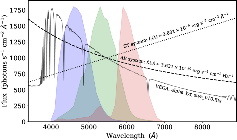
Figure 14: Comparison between the flux density (in photons s^-1 cm^-2 Å^-1) of the reference spectrum used to define the AB magnitudes (dashed black line; Eq. 14), the ST magnitudes (dotted black line; Eq. 15), and Vega magnitudes (full black line). The standard RGB spectral sensitivity curves, defined in Table 5, are shown with blue, green and red shaded areas. The units employed in this figure (known in synphot as PHOTLAM) allow a direct visual comparison with the $\langle n_{\gamma,r}\rangle$ values listed in Table 6.

For completeness, and although in this paper we strongly advocate the use of AB magnitudes, we also indicate, in the last two columns of Table 6, the expected offsets when measuring ST magnitudes, in which the reference flux densitity per unit wavelength is constant (Koornneef et al., 1986) and equal to

$$f_{r}(\lambda)=10^{-21.10/2.5}\simeq 3.6308\times 10^{-9}~{}\text{erg}~{}\text{s}^{-1}~{}\text{cm}^{-2}~{}{\text{\AA}}^{-1},$$ (15)

or when employing Vega magnitudes, using for that purpose the flux density provided by the spectrum alpha_lyr_stys_010.fits as reference. As expected, the differences between the three different systems are smaller in the $G$ band, where the corresponding reference flux densities intersect (See Fig. 14).

5.2 Synthetic RGB magnitudes for the bright star sample

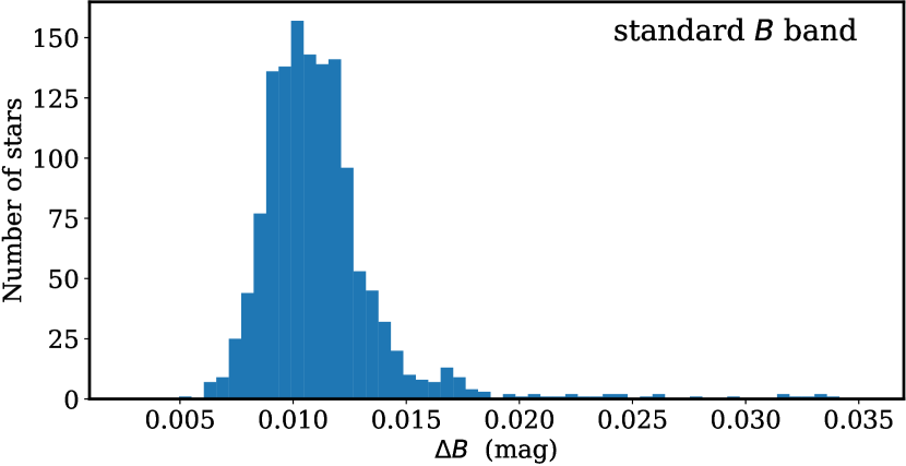
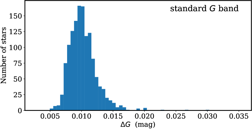
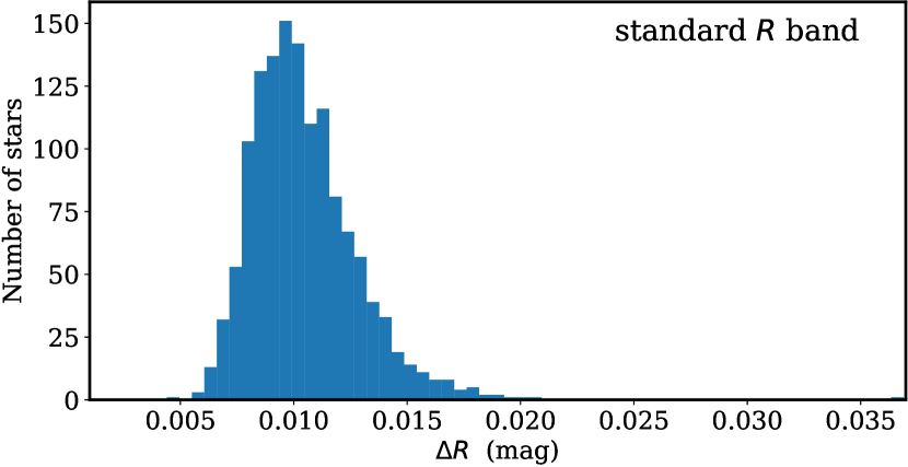
Figure 15: Distribution of random uncertainties in the synthetic standard RGB measurements performed on the final sample of fitted CK04 models, estimated from the bootstrapped spectra generated as explained in Sect. 4.2. The median values are $\Delta B=0.011$ mag (top panel), $\Delta G=0.010$ mag (middle panel) and $\Delta R=0.010$ mag (bottom panel).

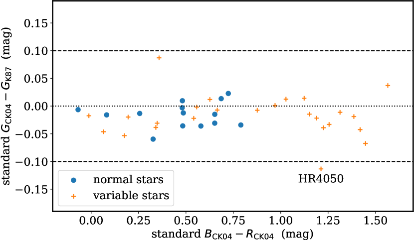
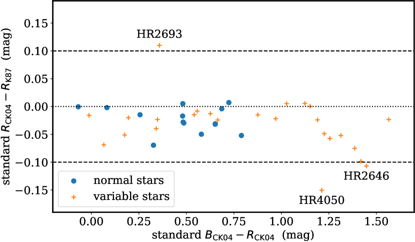
Figure 16: Differences between the synthetic RGB magnitudes computed using the best CK04 model fit and those determined from the spectra available in the K87 sample. Known variable stars are plotted with orange crosses, whereas normal stars (i.e., non-variable) are represented with blue filled circles. The horizontal dotted line in each plot marks the $\Delta{\rm mag}$=0.0 level, and the two horizontal dashed lines encompass the $\pm 0.1$ mag region. All the non-variable stars are clearly within the latter interval (the variable stars beyond the $\pm 0.1$ region have been labelled). The median and standard deviation, using the non-variable stars, are $0.000\pm 0.028$ mag for the $B$ bandpass (top panel), $-0.014\pm 0.022$ mag for the $G$ bandpass (middle panel), and $-0.023\pm 0.022$ mag for the $R$ bandpass (bottom panel).

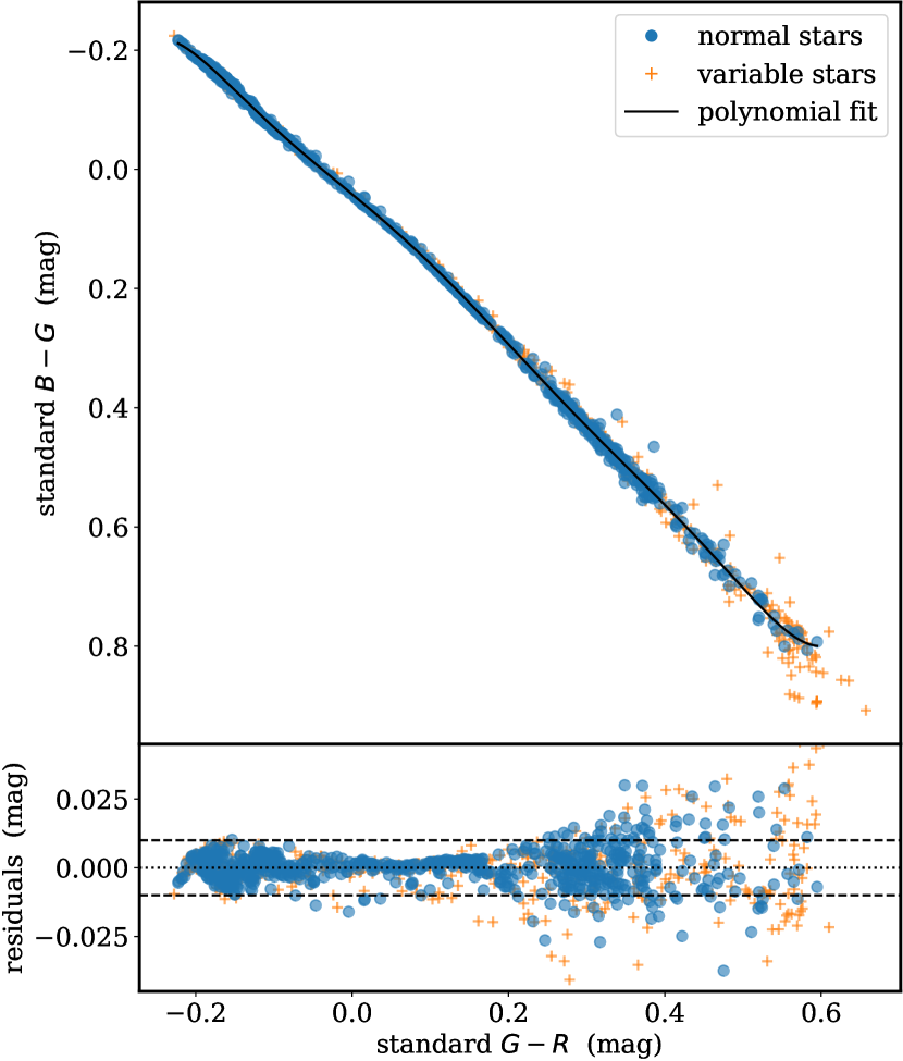
Figure 17: Color–color diagram, using the RGB magnitudes measured in the final sample of 1346 stars, using the standard photometric system defined in Sect. 5.2. The black line shows the 7-degree polynomial fit given in Eq. 5.2. The residuals around the fit are displayed in the lower panel, where the horizontal dashed lines encompass the $\pm 0.01$ mag interval. For stars with $G-R\leq 0.2$ mag, the standard deviation of the residuals is 0.004 mag for both normal (i.e. non-variable) and variable stars, whereas for stars with redder colors the standard deviations are 0.012 mag and 0.032 mag for the normal and variable stars, respectively.

Table 7: Comparison between the synthetic RGB magnitudes measured in the best CK04 fit models and those determined from the K87 flux calibrated spectra. The 39 stars are those already shown in Fig. 12. Column description: (1) HR number; (2) additional name when the star is a known variable according to Simbad; (3)–(5) synthetic RGB magnitudes (AB system), measured in the best CK04 fit, using the bandpass definitions given in Table 5, with uncertainties estimated from bootstrapping; (6)–(8) synthetic RGB magnitudes (AB system), measured in the flux calibrated K87 spectrum.

(1)	(2)	(3)		(4)		(5)		(6)	(7)	(8)
HR	Var.Name	standard $B$ (CK04)		standard $G$ (CK04)		standard $R$ (CK04)		standard $B$ (K87)	standard $G$ (K87)	standard $R$ (K87)
1325	—	4.794$\;\;\pm\;$	0.010	4.462$\;\;\pm\;$	0.009	4.215$\;\;\pm\;$	0.009	4.787	4.498	4.265
1457	alf Tau	1.758$\;\;\pm\;$	0.018	1.001$\;\;\pm\;$	0.011	0.445$\;\;\pm\;$	0.012	1.715	1.012	0.497
1654	eps Lep	3.969$\;\;\pm\;$	0.012	3.296$\;\;\pm\;$	0.012	2.819$\;\;\pm\;$	0.011	3.972	3.310	2.818
1829	NSV 2008	3.198$\;\;\pm\;$	0.013	2.866$\;\;\pm\;$	0.011	2.641$\;\;\pm\;$	0.010	3.177	2.867	2.649
1865	NSV 2128	2.566$\;\;\pm\;$	0.012	2.559$\;\;\pm\;$	0.012	2.578$\;\;\pm\;$	0.013	2.581	2.576	2.594
1983	—	3.758$\;\;\pm\;$	0.010	3.600$\;\;\pm\;$	0.008	3.502$\;\;\pm\;$	0.008	3.761	3.613	3.516
2085	—	3.804$\;\;\pm\;$	0.010	3.740$\;\;\pm\;$	0.009	3.722$\;\;\pm\;$	0.010	3.826	3.756	3.724
2326	—	$-$0.797$\;\;\pm\;$	0.011	$-$0.774$\;\;\pm\;$	0.010	$-$0.728$\;\;\pm\;$	0.010	$-$0.781	$-$0.768	$-$0.727
2646	sig CMa	4.464$\;\;\pm\;$	0.017	3.619$\;\;\pm\;$	0.013	3.017$\;\;\pm\;$	0.011	4.502	3.687	3.124
2693	NSV 3424	2.078$\;\;\pm\;$	0.011	1.861$\;\;\pm\;$	0.009	1.720$\;\;\pm\;$	0.008	2.019	1.774	1.610
2943	alf CMi A	0.481$\;\;\pm\;$	0.009	0.358$\;\;\pm\;$	0.007	0.287$\;\;\pm\;$	0.006	0.495	0.378	0.307
3153	V460 Car	6.256$\;\;\pm\;$	0.022	5.348$\;\;\pm\;$	0.013	4.691$\;\;\pm\;$	0.015	6.150	5.311	4.714
3185	rho Pup	2.884$\;\;\pm\;$	0.010	2.771$\;\;\pm\;$	0.008	2.709$\;\;\pm\;$	0.008	2.941	2.824	2.760
3188	—	4.837$\;\;\pm\;$	0.010	4.427$\;\;\pm\;$	0.009	4.151$\;\;\pm\;$	0.009	4.789	4.414	4.156
3249	NSV 3973	4.338$\;\;\pm\;$	0.012	3.643$\;\;\pm\;$	0.013	3.148$\;\;\pm\;$	0.012	4.331	3.665	3.172
3438	—	4.389$\;\;\pm\;$	0.013	4.000$\;\;\pm\;$	0.011	3.737$\;\;\pm\;$	0.010	4.409	4.031	3.769
3547	—	3.643$\;\;\pm\;$	0.011	3.216$\;\;\pm\;$	0.010	2.920$\;\;\pm\;$	0.009	3.599	3.193	2.913
3748	alf Hya	2.761$\;\;\pm\;$	0.015	2.103$\;\;\pm\;$	0.010	1.637$\;\;\pm\;$	0.011	2.730	2.089	1.632
3873	NSV 4613	3.368$\;\;\pm\;$	0.013	3.045$\;\;\pm\;$	0.011	2.827$\;\;\pm\;$	0.010	3.390	3.067	2.842
4050	V337 Car	4.226$\;\;\pm\;$	0.012	3.511$\;\;\pm\;$	0.012	3.014$\;\;\pm\;$	0.011	4.289	3.624	3.164
4114	NSV 4869	3.798$\;\;\pm\;$	0.013	3.748$\;\;\pm\;$	0.010	3.733$\;\;\pm\;$	0.009	3.805	3.795	3.802
4362	FN Leo	5.565$\;\;\pm\;$	0.017	4.731$\;\;\pm\;$	0.009	4.147$\;\;\pm\;$	0.010	5.540	4.774	4.245
4517	nu. Vir	4.873$\;\;\pm\;$	0.032	4.143$\;\;\pm\;$	0.019	3.617$\;\;\pm\;$	0.018	4.869	4.176	3.675
4540	—	3.776$\;\;\pm\;$	0.011	3.579$\;\;\pm\;$	0.009	3.450$\;\;\pm\;$	0.009	3.818	3.638	3.519
4630	eps Crv	3.719$\;\;\pm\;$	0.008	3.117$\;\;\pm\;$	0.008	2.691$\;\;\pm\;$	0.011	3.695	3.104	2.686
4763	gam Cru	2.591$\;\;\pm\;$	0.013	1.763$\;\;\pm\;$	0.014	1.205$\;\;\pm\;$	0.019	2.520	1.782	1.281
4786	bet Crv	3.082$\;\;\pm\;$	0.009	2.710$\;\;\pm\;$	0.008	2.456$\;\;\pm\;$	0.008	3.045	2.698	2.469
4932	NSV 6064	3.314$\;\;\pm\;$	0.012	2.921$\;\;\pm\;$	0.011	2.649$\;\;\pm\;$	0.011	3.285	2.928	2.673
5019	—	5.061$\;\;\pm\;$	0.011	4.774$\;\;\pm\;$	0.009	4.574$\;\;\pm\;$	0.008	5.044	4.787	4.604
5072	—	5.322$\;\;\pm\;$	0.012	5.037$\;\;\pm\;$	0.010	4.841$\;\;\pm\;$	0.009	5.299	5.027	4.836
5235	NSV 19993	2.887$\;\;\pm\;$	0.012	2.682$\;\;\pm\;$	0.010	2.546$\;\;\pm\;$	0.010	2.919	2.720	2.585
5340	alf Boo	0.573$\;\;\pm\;$	0.010	0.008$\;\;\pm\;$	0.008	$-$0.397$\;\;\pm\;$	0.010	0.520	0.007	$-$0.375
5459	—	0.039$\;\;\pm\;$	0.014	$-$0.244$\;\;\pm\;$	0.012	$-$0.441$\;\;\pm\;$	0.011	0.014	$-$0.241	$-$0.424
5854	NSV 20391	3.232$\;\;\pm\;$	0.009	2.718$\;\;\pm\;$	0.008	2.356$\;\;\pm\;$	0.010	3.219	2.726	2.371
5868	lam Ser	4.640$\;\;\pm\;$	0.014	4.431$\;\;\pm\;$	0.011	4.292$\;\;\pm\;$	0.010	4.673	4.462	4.316
6030	—	4.372$\;\;\pm\;$	0.008	3.901$\;\;\pm\;$	0.008	3.583$\;\;\pm\;$	0.008	4.397	3.935	3.635
6102	—	4.305$\;\;\pm\;$	0.012	3.925$\;\;\pm\;$	0.008	3.653$\;\;\pm\;$	0.008	4.303	3.940	3.684
6159	NSV 7812	5.644$\;\;\pm\;$	0.012	4.933$\;\;\pm\;$	0.011	4.418$\;\;\pm\;$	0.010	5.648	4.972	4.467
6623	—	3.752$\;\;\pm\;$	0.009	3.467$\;\;\pm\;$	0.008	3.269$\;\;\pm\;$	0.008	3.792	3.502	3.297

Using the median sensitivity curves defined in the previous subsection, we measured synthetic RGB magnitudes in the AB system over the final sample of 1346 CK04 models fitted to the C13 photometric data. The results are given in columns (26)–(28) of Table 2. The uncertainties in each case were derived from the standard deviations of the different values computed when using the bootstrapped spectra generated during the fitting procedure (Sect. 4.2). Histograms with these uncertainties are displayed in Fig. 15. Not surprisingly, the median uncertainties are similar to those previously found for the Johnson $B$ and $V$ filters, in particular $\Delta B=0.011$ mag, $\Delta G=0.010$ mag, and $\Delta R=0.010$ mag.

Another interesting exercise is the comparison of the synthetic RGB magnitudes with those computed using the K87 sample. The synthetic RGB magnitudes for the 39 stars in common are listed in Table 7. The differences in each bandpass, as a function of the $B-R$ color, are plotted in Fig. 16. The median and standard deviation of the differences, using only the 14 non-variable stars in this subsample, are $0.000\pm 0.028$ mag, $-0.014\pm 0.022$ mag, and $-0.023\pm 0.022$ mag, for the $B$, $G$, and $R$ bandpasses respectively. The dispersion is up to 3 times larger than the typical uncertainties previously estimated from the bootstrapping analysis, which should be at least in part attributable to the internal flux errors in the K87 spectra (already mentioned in Sect. 4.4), and we cannot discard the presence of a small systematic offset between the $G$ and $R$ measurements when comparing the CK04 and K87 spectra. In addition, most variable stars in Fig. 16 follow the same trend exhibited by the non-variable stars, with a larger dispersion towards redder colors. This behaviour is consistent with the results shown in Figs. 12 and A1, where several variable stars (plotted with orange lines) already exhibited non-negligible differences when comparing the best CK04 fitted model with the K87 spectrum.

A color–color diagram is shown in Fig. 17, where a tight correlation between the standard $B-G$ and $G-R$ colors is manifest, that can be well reproduced by the 7-degree polynomial given by

$$(B-G)= \mbox{}\;\;0.04162407+1.08718859\,(G-R)+$$

$$+0.31438309\,(G-R)^{2}+6.07961811\,(G-R)^{3}+$$

$$-10.8882237\,(G-R)^{4}-65.9762145\,(G-R)^{5}+$$

$$+216.580798\,(G-R)^{6}-174.464510\,(G-R)^{7},$$ (16)

which is valid for  $-0.22<G\!-\!R<0.59$. The residuals around this fit, computed using only the normal (i.e. non-variable) stars, exhibit a scatter well constrained within $\pm 0.01$ mag for stars with  $G-R\leq 0.2$ mag. Note, however, that the scatter increases towards redder colors, where the  $\log g$  range covered by common stars is considerably large.

5.3 Comparison between different RGB systems

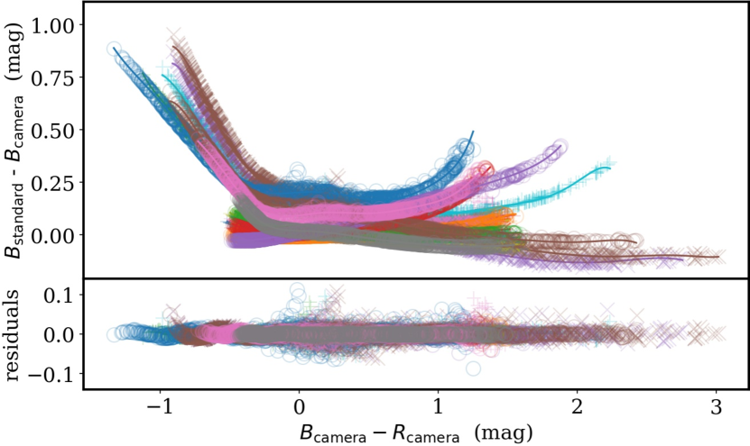
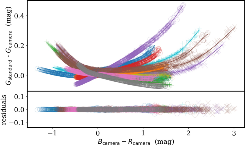
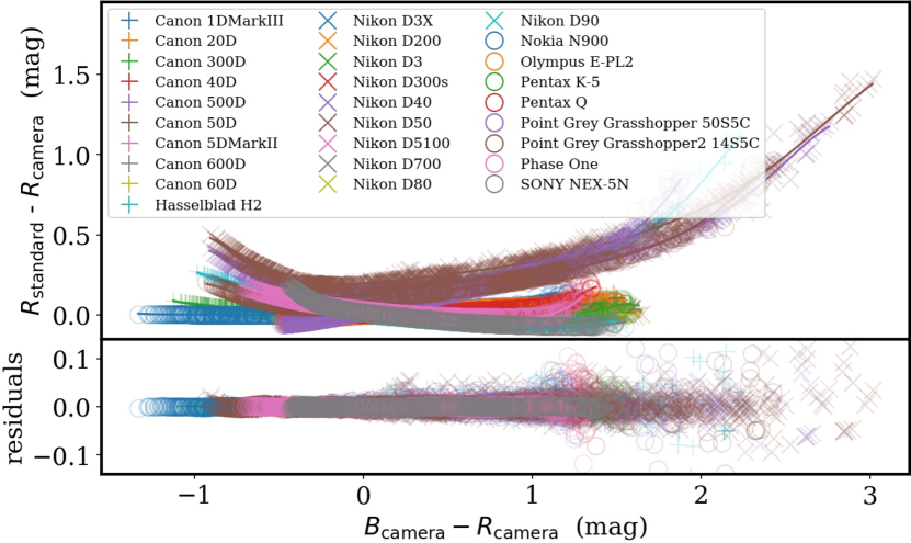
Figure 18: Differences between the RGB magnitudes computed using the median sensitivity curves of Table 5 (subindex ’standard’) and the ones determined with each one of the 28 individual sets of RGB sensitivity curves displayed in Fig. 13 (subindex ’camera’), as a function of the $B-R$ color of the considered camera. The three RGB filters are represented separately ($B$, $G$, and $R$ from top to bottom). The differences have been computed for the 1346 stars composing the final star sample listed in Table 2, and for the 28 cameras listed in the key that appears in the inset of the bottom panel. A 9-degree polynomial has been fitted to each filter and camera (continuous lines; polynomial coefficients given in Appendix B), while the fit residuals are displayed at the bottom panel of each filter plot.

In order to test the potential usability of the standard RGB system defined with the median sensitivity curves, it is important to check how easy will be the transformation from RGB magnitudes measured with a typical camera, to the mentioned standard system. For that purpose, we computed the synthetic RGB magnitudes over the whole final sample of 1346 stars, using the 28 sets of RGB filters compiled by Jiang et al. (2013) and displayed in Fig. 13.

In Fig. 18 we represent the difference between the RGB magnitudes computed using the median spectral sensitivity curves provided in Table 5 and the ones measured with each of the 28 individual camera sets. In most cases, the differences are of the order of a few tenths of a magnitude, although larger corrections are necessary for the bluest stars in the $B$ band and for the reddest stars in the $R$ band. Without entering into unnecessary details, this behaviour is not surprising considering the variations of the different RGB sensitivity curves in Fig. 13. It is important to emphasize here that, more important than how large the differences between a particular RGB filter set and the standard RGB system are, the relevant result is that these differences can be reasonably well modelled by smooth polynomials. For illustration, the displayed data for each filter and camera have been fitted using a 9-degree polynomial, overplotted as continuous line with the same color as the one chosen for each RGB set, with the fit residuals displayed at the bottom plot of all the panels. The resulting polynomial coefficients for 28 considered cameras are listed in Table B1, together with the median and standard deviation of the residuals. In most cases, the residuals scatter is below 0.01 mag. Based on these results, we conclude that observations performed with most cameras can be transformed into the standard RGB system by using smooth polynomial fits.

6 Conclusions

The availability of a catalogue of bright standard stars with RGB magnitudes, measured in a well-defined photometric system, is essential to scientifically exploit the large amount of data that at present can be gathered with high-quality and inexpensive digital cameras equipped with Bayer-like color filters.

For the work presented in this paper we have used high-quality 13 medium-narrow-band photometric data to fit stellar atmosphere models, in order to obtain spectral energy distributions for bright stars. The reliability of these fits has been checked by comparing the synthetic Johnson $B$ and $V$ magnitudes computed on the fitted models with the corresponding data available through the Simbad database. This comparison has shown that the $\pm 3\sigma$ scatter in both bands is around or below 0.10 mag, being part of this dispersion attributable to the heterogenous source compilation in the Simbad data. The initial star sample, composed by 1522 objects, was cleaned by removing bad fits and stars with discrepant Johnson $B$ and $V$ magnitudes, reducing the final sample to 1346 objects. As an additional check, we have compared a subset of 39 fitted models with actual absolute flux calibrated spectra from the literature, which revealed that the typical standard deviation in the fitted 13 photometric bandpasses is 0.05 mag, being part of this dispersion attributable to the flux calibrated spectra. Furthermore, the fitted 13 band fluxes for each star were randomly modified (assuming typical uncertainties of 0.02 mag) in order to generate bootstrapped versions of the fitted models.

The whole set of fitted star models, that constitute the UCM library of spectrophotometric standards, together with their associated bootstrapped versions, have been employed to compute synthetic RGB magnitudes and uncertainties. Prior to this step, a new RGB photometric system, that can be used as a standard reference, has been established, by defining standard RGB sensitivity curves as the median of the corresponding curves of 28 commercial cameras. The typical random uncertainties in the synthetic RGB magnitudes, computed only from the bootstrapped spectra, are close to $0.01$ mag. These uncertainties are 3 times larger when we compare the synthetic RGB magnitudes with the corresponding values in the subsample of 39 stars with flux calibrated spectra. However, the unaccounted uncertainties in the flux calibrated data should have a contribution to this budget. In addition, we cannot discard a small systematic deviation of $-0.01$ and $-0.03$ mag in the $G$ and $R$ bandpasses, although these numbers rely on the analysis of only 14 non-variable stars.

The feasibility of using the new RGB photometric bandpasses defined in this work as a standard RGB system, has been demonstrated by computing simple polynomial transformations that model the differences between the RGB magnitudes derived employing the standard system and the ones obtained using 28 individual sets of RGB sensitivity curves of real cameras, with a typical scatter around these polynomial fits within 0.01 mag.

Since non-variable stars constitue ideal radiometric references, one immediate application of this work is the transformation of the sky in an accessible and free laboratory for the proper calibration of the high volume of already existing (and future) digital cameras. Obviously, a proper calibration will require the corresponding observational effort and subsequent data reduction and analysis, but the repeatability of measurements should facilitate to reach calibration accuracies comparable with those achievable in radiometric laboratories. It is important to emphasize that the synthetic stellar library include a non-negligible number of variable stars (594 out of 1346 objects), but they have been kept in the final sample because they did not present discrepant $B$ and $V$ magnitudes in the Simbad database. In any case, their use and validity should be subject to a careful analysis.

We hope that the catalogue of 1346 flux calibrated stellar spectra presented here, that by itself already constitutes a library of bright spectrophotometric standards suitable for spectroscopic calibrations, and the corresponding synthetic RGB magnitudes, can be used as a reference for future work on several astronomical fields, where the collaboration of many observers equipped with high-quality digital cameras may provide data that facilitate the research advancement. In addition, this could help to make citizen science a reality in the realm of astronomy, increasing the public’s interest and understanding of science, highlighting the fact that scientific research matters.

Data Availability

The work in this paper has made use of the photometric data published by Johnson & Mitchell (1975, Table 7, available online), Schuster (1976, Table 1), Bravo Alfaro et al. (1997, Table 1), the Stellar Atmopshere Models of Castelli & Kurucz (2003), as provided by the STScI web page, the database of camera spectral sensitivity database of Jiang et al. (2013, available online), the Bright Star Catalogue (Hoffleit, 1964, available online), and the General Catalogue of Variable Stars (Samus’ et al., 2017, available online).

The supplementary material described as Appendices A and B is available online only.

All the results of this paper, together with future additional material, will be available online at http://guaix.ucm.es/rgbphot.

References

- Alcaino (1965) Alcaino G., 1965, Lowell Observatory Bulletin, 6, 167
- Alvarez & Schuster (1978) Alvarez M., Schuster W. J., 1978, in Bulletin of the American Astronomical Society. p. 687
- Alvarez & Schuster (1982) Alvarez M., Schuster W. J., 1982, Rev. Mex. Astron. Astrofis., 5, 173
- Astropy Collaboration et al. (2013) Astropy Collaboration et al., 2013, A&A, 558, A33
- Astropy Collaboration et al. (2018) Astropy Collaboration et al., 2018, AJ, 156, 123
- Bará et al. (2019) Bará S., Rodríguez-Arós A., Pérez M., Tosar B., Lima R., de Miguel A. S., Zamorano J., 2019, Lighting Research & Technology, 51, 1092
- Bertolo et al. (2019) Bertolo A., Binotto R., Ortolani S., Sapienza S., 2019, Journal of Imaging, 5, 56
- Bessell & Murphy (2012) Bessell M., Murphy S., 2012, PASP, 124, 140
- Blackford (2016) Blackford M., 2016, The AAVSO DSLR Observing Manual. American Association of Variable Star Observers, https://www.aavso.org/sites/default/files/publications_files/dslr_manual/AAVSO_DSLR_Observing_Manual_V1.4.pdf
- Bohlin et al. (2014) Bohlin R. C., Gordon K. D., Tremblay P. E., 2014, PASP, 126, 711
- Bouroussis & Topalis (2020) Bouroussis C. A., Topalis F. V., 2020, Journal of Quantitative Spectroscopy and Radiative Transfer, 253, 107155
- Bravo Alfaro et al. (1993) Bravo Alfaro H., Arellano Ferro A., Schuster W. J., 1993, Rev. Mex. Astron. Astrofis., 26, 100
- Bravo Alfaro et al. (1997) Bravo Alfaro H., Arellano Ferro A., Schuster W. J., 1997, PASP, 109, 958
- Cardiel (1999) Cardiel N., 1999, PhD thesis, Universidad Complutense de Madrid, https://ui.adsabs.harvard.edu/abs/1999PhDT........12C
- Casagrande & VandenBerg (2014) Casagrande L., VandenBerg D. A., 2014, MNRAS, 444, 392
- Castelli & Kurucz (2003) Castelli F., Kurucz R. L., 2003, in Piskunov N., Weiss W. W., Gray D. F., eds, IAU Symposium Vol. 210, Modelling of Stellar Atmospheres. p. A20 (arXiv:astro-ph/0405087)
- Chavarria-K. & de Lara (1981) Chavarria-K. C., de Lara E., 1981, Rev. Mex. Astron. Astrofis., 6, 159
- Conconi & Mantegazza (1985) Conconi P., Mantegazza L., 1985, in Hayes D. S., Pasinetti L. E., Philip A. G. D., eds, IAU Symposium Vol. 111, Calibration of Fundamental Stellar Quantities. pp 553–556
- Dobler et al. (2015) Dobler G., et al., 2015, Information Systems, 54, 115
- Ducati (2002) Ducati J. R., 2002, VizieR Online Data Catalog,
- Fabricius et al. (2002) Fabricius C., Høg E., Makarov V. V., Mason B. D., Wycoff G. L., Urban S. E., 2002, A&A, 384, 180
- Gural & Šegon (2009) Gural P., Šegon D., 2009, WGN, Journal of the International Meteor Organization, 37, 28
- Hänel et al. (2018) Hänel A., et al., 2018, Journal of Quantitative Spectroscopy and Radiative Transfer, 205, 278
- Harris et al. (2020) Harris C. R., et al., 2020, Nature, 585, 357
- Hernández et al. (2014) Hernández J., et al., 2014, ApJ, 794, 36
- Hoffleit (1964) Hoffleit D., 1964, Catalogue of Bright Stars. Yale University Observatory
- Høg et al. (2000) Høg E., et al., 2000, A&A, 355, L27
- Hsu et al. (2013) Hsu W.-H., Hartmann L., Allen L., Hernández J., Megeath S. T., Tobin J. J., Ingleby L., 2013, ApJ, 764, 114
- Hunter (2007) Hunter J. D., 2007, Computing in Science Engineering, 9, 90
- Jechow (2019) Jechow A., 2019, Sustainability, 11, 750
- Jechow & Hölker (2019) Jechow A., Hölker F., 2019, Journal of Imaging, 5, 69
- Jechow et al. (2018) Jechow A., Ribas S. J., Domingo R. C., Hölker F., Kolláth Z., Kyba C. C., 2018, Journal of Quantitative Spectroscopy and Radiative Transfer, 209, 212
- Jechow et al. (2019a) Jechow A., Kyba C. C. M., Hölker F., 2019a, Journal of Imaging, 5, 46
- Jechow et al. (2019b) Jechow A., Hölker F., Kyba C. C. M., 2019b, Scientific Reports, 9, 1391
- Jiang et al. (2013) Jiang J., Liu D., Gu J., Süsstrunk S., 2013, in 2013 IEEE Workshop on Applications of Computer Vision (WACV). pp 168–179
- Johnson & Mitchell (1975) Johnson H. L., Mitchell R. I., 1975, Rev. Mex. Astron. Astrofis., 1, 299
- Johnson et al. (1966) Johnson H. L., Mitchell R. I., Iriarte B., Wisniewski W. Z., 1966, Communications of the Lunar and Planetary Laboratory, 4, 99
- Johnson et al. (1967) Johnson H. L., Mitchell R. I., Latham A. S., 1967, Communications of the Lunar and Planetary Laboratory, 6, 85
- Joner et al. (2006) Joner M. D., Taylor B. J., Laney C. D., van Wyk F., 2006, AJ, 132, 111
- Kiehling (1987) Kiehling R., 1987, A&AS, 69, 465
- Kolláth et al. (2020) Kolláth Z., Cool A., Jechow A., Kolláth K., Száz D., Tong K. P., 2020, Journal of Quantitative Spectroscopy and Radiative Transfer, 253, 107162
- Koornneef et al. (1986) Koornneef J., Bohlin R., Buser R., Horne K., Turnshek D., 1986, Highlights of Astronomy, 7, 833
- Kuechly et al. (2012) Kuechly H. U., Kyba C. C., Ruhtz T., Lindemann C., Wolter C., Fischer J., Hölker F., 2012, Remote Sensing of Environment, 126, 39
- Kyba (2019) Kyba C., 2019, Loss of the Night citizen science project. http://lossofthenight.blogspot.com/2019/09/first-action-of-nachtlicht-buhne-lamp.html
- Kyba et al. (2014) Kyba C. C. M., Garz S., Kuechly H., de Miguel A. S., Zamorano J., Fischer J., Hölker F., 2014, Remote Sensing, 7, 1–23
- Lim (2018) Lim P. L., 2018, stsynphot, https://doi.org/10.5281/zenodo.3247832
- Lodén (1967) Lodén L. O., 1967, Arkiv for Astronomi, 4, 375
- Lodén (1968) Lodén L. O., 1968, Arkiv for Astronomi, 4, 425
- Lodén (1969a) Lodén L. O., 1969a, Arkiv for Astronomi, 5, 149
- Lodén (1969b) Lodén L. O., 1969b, Arkiv for Astronomi, 5, 161
- Lodén & Nordström (1969) Lodén L. O., Nordström B., 1969, Arkiv for Astronomi, 5, 231
- Marx & Lehmann (1979) Marx S., Lehmann H., 1979, Astronomische Nachrichten, 300, 295
- Mason et al. (2001) Mason B. D., Wycoff G. L., Hartkopf W. I., Douglass G. G., Worley C. E., 2001, AJ, 122, 3466
- Meier (2018) Meier J. M., 2018, International Journal of Sustainable Lighting, 20, 11
- Mitchell & Johnson (1969) Mitchell R. I., Johnson H. L., 1969, Communications of the Lunar and Planetary Laboratory, 8, 1
- Moehler et al. (2014) Moehler S., et al., 2014, A&A, 568, A9
- Mousis et al. (2014) Mousis O., et al., 2014, Experimental Astronomy, 38, 91
- Nelder & Mead (1965) Nelder J. A., Mead R., 1965, The Computer Journal, 7, 308
- Newville et al. (2014) Newville M., Stensitzki T., Allen D. B., Ingargiola A., 2014, LMFIT: Non-Linear Least-Square Minimization and Curve Fitting for Python, http://dx.doi.org/10.5281/zenodo.11813
- Nicolet (1978) Nicolet B., 1978, A&AS, 34, 1
- Nisselson et al. (2017) Nisselson E., Hunter-Syed A., Shah S., 2017, 45 Billion Cameras by 2020 Fuel Business Opportunities. LDV Capital, https://www.ldv.co/blog/2017/8/8/45-billion-cameras-by-2022-fuel-business-opportunities
- Oja (1985) Oja T., 1985, A&AS, 61, 331
- Oja (1991) Oja T., 1991, A&AS, 89, 415
- Oja (1993) Oja T., 1993, A&AS, 100, 591
- Oke & Gunn (1983) Oke J. B., Gunn J. E., 1983, ApJ, 266, 713
- Pérez & Granger (2007) Pérez F., Granger B. E., 2007, Computing in Science and Engineering, 9, 21
- Petford & Blackwell (1989) Petford A. D., Blackwell D. E., 1989, A&AS, 78, 511
- Rakos et al. (1982) Rakos K. D., et al., 1982, A&AS, 47, 221
- Röser et al. (2011) Röser S., Schilbach E., Piskunov A. E., Kharchenko N. V., Scholz R. D., 2011, A&A, 531, A92
- STScI development Team (2018) STScI development Team 2018, synphot: Synthetic photometry using Astropy (ascl:1811.001), https://synphot.readthedocs.io/en/latest/
- Samus’ et al. (2017) Samus’ N. N., Kazarovets E. V., Durlevich O. V., Kireeva N. N., Pastukhova E. N., 2017, Astronomy Reports, 61, 80
- Sánchez de Miguel et al. (2019) Sánchez de Miguel A., Kyba C. C., Aubé M., Zamorano J., Cardiel N., Tapia C., Bennie J., Gaston K. J., 2019, Remote Sensing of Environment, 224, 92
- Sánchez de Miguel et al. (2020) Sánchez de Miguel A., Kyba C. C. M., Zamorano J., Gallego J., Gaston K. J., 2020, Scientific Reports, 10, 7829
- Schuster (1976) Schuster W. J., 1976, Rev. Mex. Astron. Astrofis., 1, 327
- Schuster (1979a) Schuster W. J., 1979a, Rev. Mex. Astron. Astrofis., 4, 233
- Schuster (1979b) Schuster W. J., 1979b, Rev. Mex. Astron. Astrofis., 4, 301
- Schuster (1979c) Schuster W. J., 1979c, Rev. Mex. Astron. Astrofis., 4, 307
- Schuster (1982a) Schuster W. J., 1982a, Rev. Mex. Astron. Astrofis., 5, 137
- Schuster (1982b) Schuster W. J., 1982b, Rev. Mex. Astron. Astrofis., 5, 149
- Schuster (1984) Schuster W. J., 1984, Rev. Mex. Astron. Astrofis., 9, 53
- Schuster & Alvarez (1983) Schuster W. J., Alvarez M., 1983, PASP, 95, 35
- Schuster & Guichard (1984) Schuster W. J., Guichard J., 1984, Rev. Mex. Astron. Astrofis., 9, 141
- Schuster & Guichard (1985) Schuster W. J., Guichard J., 1985, Rev. Mex. Astron. Astrofis., 11, 7
- Squires (2001) Squires G. L., 2001, Practical Physics, 4 edn. Cambridge University Press
- Stefanov et al. (2017) Stefanov W. L., Evans C. A., Runco S. K., Justin Wilkinson M., Higgins M. D., Willis K., 2017, Handbook of Satellite Applications, pp 847 – 899
- Virtanen et al. (2020) Virtanen P., et al., 2020, Nature Methods, 17, 261
- Wolfe (1998) Wolfe W. L., 1998, Introduction to Radiometry. SPIE Press, https://spie.org/Publications/Book/287476
- Yoss & Griffin (1997) Yoss K. M., Griffin R. F., 1997, Journal of Astrophysics and Astronomy, 18, 161
- Zacharias et al. (2012) Zacharias N., Finch C. T., Girard T. M., Henden A., Bartlett J. L., Monet D. G., Zacharias M. I., 2012, VizieR Online Data Catalog, p. I/322A
- Zamorano (2020) Zamorano J., 2020, AZOTEA: monitoring the night sky during and after isolation. Universidad Complutense de Madrid, https://guaix.ucm.es/wp-content/uploads/2020/05/AZOTEA_English_manual_V2.pdf
- Zheng et al. (2018) Zheng Q., Weng Q., Huang L., Wang K., Deng J., Jiang R., Ye Z., Gan M., 2018, Remote Sensing of Environment, 215, 300
- van Belle & von Braun (2009) van Belle G. T., von Braun K., 2009, ApJ, 694, 1085
- van der Sluys (2005) van der Sluys M., 2005, Constellation lines, https://github.com/hemel-waarnemen-com/Constellation-lines