Energy Efficient Edge Computing: When Lyapunov Meets Distributed Reinforcement Learning

Abstract

In this work, we study the problem of energy-efficient computation offloading enabled by edge computing. In the considered scenario, multiple users simultaneously compete for limited radio and edge computing resources to get offloaded tasks processed under a delay constraint, with the possibility of exploiting low power sleep modes at all network nodes. The radio resource allocation takes into account inter- and intra-cell interference, and the duty cycles of the radio and computing equipment have to be jointly optimized to minimize the overall energy consumption. To address this issue, we formulate the underlying problem as a dynamic long-term optimization. Then, based on Lyapunov stochastic optimization tools, we decouple the formulated problem into a CPU scheduling problem and a radio resource allocation problem to be solved in a per-slot basis. Whereas the first one can be optimally and efficiently solved using a fast iterative algorithm, the second one is solved using distributed multi-agent reinforcement learning due to its non-convexity and NP-hardness. The resulting framework achieves up to $96.5\%$ performance of the optimal strategy based on exhaustive search, while drastically reducing complexity. The proposed solution also allows to increase the network’s energy efficiency compared to a benchmark heuristic approach.

I Introduction

Wireless communication networks are experiencing an unprecedented revolution, evolving from pure communication systems towards a tight integration of communication, computation, caching, and control [1]. Such a heterogeneous ecosystem requires a flexible network design and orchestration, able to accommodate on the same network infrastructure all the different services with their requirements in terms of energy, latency, and reliability. This requires an enhancement of the radio access network, e.g., through the adoption of millimeter wave (mmWave) communications, densification of access points (APs), and a flexible management of the physical layer [2]. In addition, the deployment of computing and storage capabilities at the network edge will enable network function virtualization and a fast processing of the myriad of data collected by sensors, cars, mobile devices, etc. For this, Edge Computing was conceived to enable energy efficient, low-latency, highly reliable services by bringing cloud resources close to the users.

In this context, dynamic computation offloading allows resource-poor devices to transfer application execution to Edge Servers (ESs) to reduce energy consumption and/or latency. From a network management perspective, this task is complex and requires the joint optimization of radio and computation resources. This problem has received wide attention[3]. In [4], a scheduling strategy is proposed to counterbalance task completion ratio and throughput, hinging on Lyapunov optimization. [5] aims at minimizing the long-term average delay under a long-term average power consumption constraint. In [6], the long-term average energy consumption of a MEC network is minimized under a delay constraint, using a MEC sleep control. [7] minimizes the energy consumption under a mean service delay constraint, optimizing the number of active base stations and the ESs’ computation resource allocation, leveraging sleep modes for APs and ESs. In [8], Lyapunov optimization is used to reduce the energy consumption of a fog network, guaranteeing an average response time. In [9], devices’ and APs’ energy consumption is minimized via Lyapunov optimization, Lagrange multipliers and sub-gradient techniques, using APs’ sleep state, under latency constraints.

Recently, the advances of machine learning and Deep Reinforcement Learning (DRL) in wireless networks have opened up new possibilities for low-complexity and efficient algorithms for MEC [1], especially when model-based optimization is challenged by the difficulty or even impossibility of writing mathematical models that accurately predict the networks’ behavior. In this sense, the authors of [10] propose to couple model-based Lyapunov optimization with model-free DRL and formulate a sum-rate maximization problem under queue stability and long-term device energy constraints. However, their reference scenario considers a single AP, and no CPU scheduling is optimized at the ES. [11] also considers the same approach, with the aim of minimizing the sum of the power consumption of the edge nodes, and a cost charged by a central cloud to help the edge node in processing the tasks under stability constraints. However, they do not consider the energy consumption of end users and APs.

In this paper, we combine the convenience of a model-based solution that exploits Lyapunov stochastic optimization, with the power of model-free solutions based on multi-agent reinforcement learning (MARL), aiming at energy efficient computation offloading from an overall network perspective. We consider multiple user equipments (UEs) that perform computation offloading and compete for computation resources at an ES and for radio resources, interfering onto each other’s transmissions. We treat the problem as a long-term system energy minimization with average end-to-end delay constraints, in a network with multiple APs and one ES, all exploiting low-power sleep operation modes. Although we do not assume any knowledge on radio channels and data arrival statistics, our online solution optimizes in each time slot the UE-AP association in a distributed way, and the ES’s CPU scheduling via a fast iterative algorithm whose solution’s complexity scales linearly in the number of UEs.

Compared to the cited works, the originality of our strategy consists in simultaneously: $i)$ minimizing the duty cycles of all the network elements under delay constraints; $ii)$ effectively managing radio interference; $iii)$ being low-complexity; $iv)$ combining Lyapunov optimization with DRL; $v)$ being distributed and compatible with UE’s mobility. The latter point, in sharp contrast with [10], results from the zero-shot generalization capability of our solution: it optimizes the learned computation offloading policy for all possible deployments of UEs using attention neural networks, and adapts when the number of UEs differs from the initial training point.

II System Model

We consider the scenario of Fig. 1, where $K$ UEs offload computational tasks to an ES, via one out of $N$ possible APs. Let $\mathcal{U}$ and $\mathcal{A}$ be the sets of UEs and APs, respectively. Also, let $\mathcal{A}_{k}$ be the set of APs UE $k$ can be associated with. In our dynamic system, time is divided in slots of equal duration $\tau$. Specifically, we assume that a fraction $\beta\in(0,1)$ of each slot is devoted to control signaling and ($1-\beta$) to data transmission and computation, both potentially happening simultaneously. At each time slot $t$, radio channels and data arrivals at the UEs vary according to a priori unknown statistics. Consequently, the achievable data rate over the radio channels and the computation rate at the ES vary with time.

II-A Radio access and data rate model

In this paper, we consider uplink communications for computation offloading. Specifically, we assume spatial division multiple access. All UEs are served by the APs over the same time-frequency resources but with different beams. In this scenario, uplink communications are affected by both intra- and inter-cell interference. Indeed, suppose that UE $k$ is served by AP $n$ at time $t$. Let $p_{k}^{u,\rm tx}(t)$ be the uplink transmit power of UE $k$, $G_{kn}^{\rm ch}(t)$ the channel power gain between UE $k$ and AP $n$, $G_{kn}^{\rm tx}(t)$ the transmit antenna gain towards the direction of AP $n$, $G_{kn}^{\rm rx}(t)$ the receive antenna gain, $B$ the allocated bandwidth, and $N_{0}$ the noise power spectral density. Then, the signal-to-interference-plus-noise ratio (SINR) is given by

$$\textrm{SINR}_{k}(t)=\frac{p_{k}^{u,\rm tx}(t)G_{kn}^{\rm tx}(t)G_{kn}^{\rm ch}(t)G_{kn}^{\rm rx}(t)}{\mathcal{I}_{kn}(t)+N_{0}B},$$

where $\mathcal{I}_{kn}(t)=\sum\nolimits_{k^{\prime}\in\mathcal{U}\setminus\{k\}}p_{k^{\prime}}^{u,\rm tx}(t)G_{k^{\prime}n}^{\rm tx}(t)G_{k^{\prime}n}^{\rm ch}(t)G_{k^{\prime}n}^{\rm rx}(t)$ is the overall interference. Then, the achievable rate of UE $k$ at time $t$ is $R_{k}(t)=B\log_{2}(1+\textrm{SINR}_{k}(t))$. If the $k$-th UE’s offloadable data unit is encoded into $S_{k}$ bits, the number of data units transmitted in the uplink direction at time $t$ is

$$N_{k}^{u}(t)=\left\lfloor\frac{(1-\beta)\tau R_{k}(t)}{S_{k}}\right\rfloor.$$ (1)

II-B Computation model

At the ES, all UEs are served by one core and compete for the CPU time in each time slot. Given a core frequency $f_{c}(t)$ (measured in CPU cycles per second), each UE is allocated a portion $f_{k}(t)$ of $f_{c}(t)$, with $\sum_{k=1}^{K}f_{k}(t)\leq f_{c}(t)$. Then, denoting by $J_{k}$ the number of processed data units per CPU cycle, the number of data units processed over one slot is

$$N_{k}^{c}(t)=\lfloor(1-\beta)\tau f_{k}(t)J_{k}\rfloor.$$ (2)

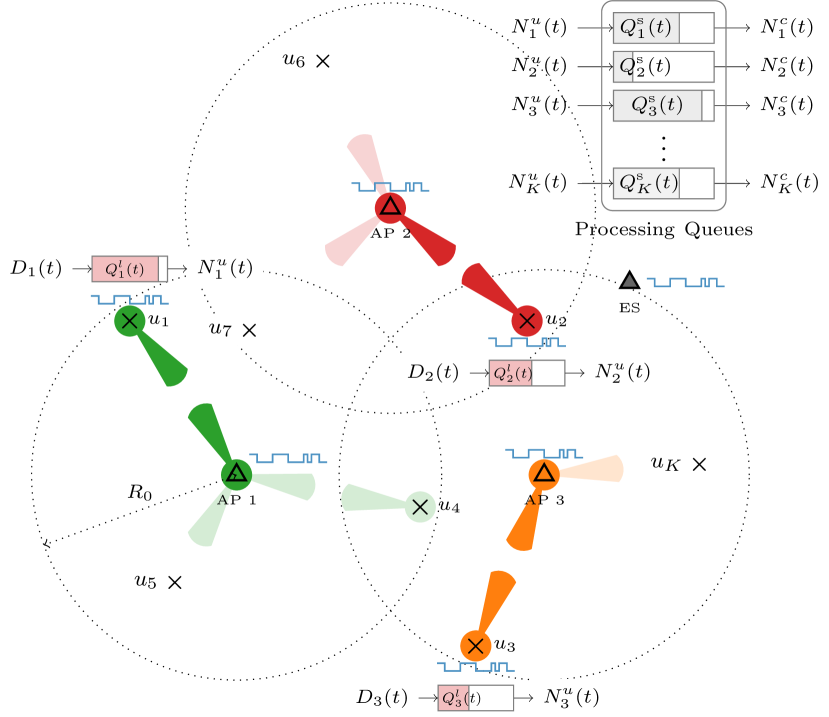
Figure 1: Network model with 3 APs deployed with $K$ UEs.

II-C Delay and queuing model

In our setting, computation offloading involves two steps: $i)$ an uplink transmission phase of input data from the UEs; $ii)$ a computation phase at the ES. New data units are continuously generated from an application at the UE’s side and consequently offloaded and processed at the ES. In particular, once generated, data are queued locally at the UEs, then uploaded to the ES through one AP with time varying data rate as in (1). At the ES, they are queued waiting to be processed and they are finally computed with time varying computational rate as in (2). Thus, we represent the overall system through a simple queuing model involving both queues, synthetically depicted in Fig. 1. Accordingly, each data unit experiences two different delays: $i)$ a communication delay, including buffering at the UE; $ii)$ a computation delay, including buffering at the ES. As shown later, we take into account these two delays jointly, as in [12]. UE $k$’s uplink communication queue evolves as $Q_{k}^{l}(t+1)=\max\left(0,Q_{k}^{l}(t)-N_{k}^{u}(t)\right)+D_{k}(t)$, where $D_{k}(t)$ is the number of newly arrived offloadable data units generated by the application at the UE at time $t$, which is the realization of a random process whose statistics are unknown a priori. The remote computation queue at the ES evolves as $Q_{k}^{\rm s}(t+1)=\max(0,Q_{k}^{\rm s}(t)-N_{k}^{c}(t))+\min(Q_{k}^{l}(t),N_{k}^{u}(t)).$

End-to-end delay constraints. By Little’s law [13], given a stationary queueing system, the average overall service delay is proportional to the average queue length. Then, in our system, the overall delay is directly related to the sum of the uplink communication queue and the computation queue $Q_{k}^{\text{tot}}(t)=Q_{k}^{l}(t)+Q_{k}^{\rm s}(t)$. In particular, if $\displaystyle\bar{D}_{k}=\mathbb{E}\left\{D_{k}(t)/\tau\right\}$ is the average data unit arrival rate, the long-term average end-to-end delay $L_{k}^{\rm avg}$ experienced by a data unit generated by UE $k$ is given by the ratio between the average of $Q_{k}^{\rm tot}$ and the average arrival rate. Thus, our constraint on the long-term average delay $L_{k}^{\textrm{avg}}$ is formulated as follows:

$$\lim_{T\to\infty}\frac{1}{T}\sum_{t=1}^{T}\mathbb{E}\left\{Q_{k}^{\rm tot}(t)\right\}\leq Q_{k}^{\textrm{avg}}=L_{k}^{\textrm{avg}}\bar{D}_{k},\quad\forall k.$$ (3)

Note: $\bar{D}_{k}$ is not known a priori, but can be estimated online.

II-D Energy consumption model

We exploit low-power operation modes at UEs, APs, and ES to reduce the overall energy consumption. However, due to control signaling, UEs, APs, and ES are active for at least $\beta\tau$ seconds in each slot, consuming active power. Hence, the energy consumption of each entity is modeled as follows:

UE Energy Consumption. Let $x_{k,n}(t)\in\{0,1\}$ be an association variable equal to $1$ if and only if UE $k$ offloads its data via AP $n$ at time $t$. Let $p_{k}^{\rm u,off}$ and $p_{k}^{\rm u,on}$ be UE $k$’s sleep and active power, respectively. Then, the total UEs’ energy consumption at time $t$ is:

$${\rm E}_{\rm u}(t) = \sum_{k=1}^{K}\tau\bigg{[}(1-\beta)\bigg{(}I_{k}^{\rm u}(t)\left(p_{k}^{\rm u,on}+p_{k}^{\rm u,tx}(t)\right)$$ (4)

$$\qquad\qquad+(1-I_{k}^{\rm u}(t))p_{k}^{\rm u,off}\bigg{)}+\beta p_{k}^{\rm u,on}\bigg{]},$$

where $\displaystyle I_{k}^{\rm u}(t)=\max_{n\in\mathcal{A}_{k}}\{x_{k,n}(t)\}$ indicates if UE $k$ is active: if it does not transmit at time $t$, $I_{k}^{\rm u}(t)=0$, and $p_{k}^{\rm u,tx}(t)=0$.

AP Energy Consumption. Let $p_{n}^{\rm a,off}$ and $p_{n}^{\rm a,on}$ be the $n$-th AP’s sleep and active power consumption, respectively. The total APs’ energy consumption at time $t$ is

$${\rm E}_{\rm a}(t) = \sum_{n=1}^{N}\tau\bigg{[}(1-\beta)\left(I_{n}^{\rm a}(t)p_{n}^{\rm a,on}+(1-I_{n}^{\rm a}(t))p_{n}^{\rm a,off}\right)$$ (5)

$$\qquad\qquad+\beta p_{n}^{\rm a,on}\bigg{]},$$

where $\displaystyle I_{n}^{\rm a}(t)=\max_{k\in\mathcal{U}}\{x_{k,n}(t)\}$ indicates whether AP $n$ is active ($I_{n}^{\rm a}(t)=1$) or not ($I_{n}^{\rm a}(t)=0$).

ES Energy Consumption. To reduce the energy consumption, we adopt both a low-power sleep mode for the ES, when no computation is performed at a given slot $t$, and a scaling of the CPU frequency $f_{c}(t)$, when the CPU is active and computing [14]. Namely, the CPU core consumes a power $p_{\rm s}^{\rm on}$ in active state, and a power $p_{\rm s}^{\rm off}<p_{\rm s}^{\rm on}$ in sleep state. When the ES is active, the dynamic power spent for computation is $p_{\rm s}^{\rm c}(t)=\kappa f_{c}^{3}(t)$, where $\kappa$ is the effective switched capacitance of the processor [15]. In particular, we assume that $f_{c}(t)$ can be dynamically selected from a finite set $\mathcal{F}=\{0,\ldots,f_{\max}\}$. Therefore, the ES’s energy consumption at time $t$ is

$${\rm E}_{\rm s}(t) = (1-\beta)\tau\left(I_{\rm s}(t)\left(p_{\rm s}^{\rm on}+p_{\rm s}^{\rm c}(t)\right)+(1-I_{\rm s}(t))p_{\rm s}^{\rm off}\right)$$ (6)

$${~{}}+\beta\tau p_{\rm s}^{\rm on},$$

where $I_{\rm s}(t)=\mathbf{1}\{f_{c}(t)\}$, with $\mathbf{1}\{\cdot\}$ the indicator function, indicates whether the ES is active ($I_{\rm s}(t)=1$) or not ($I_{\rm s}(t)=0$). From (4), (5), (6), the total system energy consumption at time $t$ is ${\rm E}_{\rm tot}(t)={\rm E}_{\rm s}(t)+{\rm E}_{\rm a}(t)+{\rm E}_{\rm u}(t)$. Our objective function is a convex combination of its terms:

$${\rm E}_{\rm w}(t)=\alpha_{1}{\rm E}_{\rm u}(t)+\alpha_{2}{\rm E}_{\rm a}(t)+\alpha_{3}{\rm E}_{\rm s}(t),$$ (7)

with $\sum_{i=1}^{3}\alpha_{i}=1$. Different $\alpha_{i}$ lead to different strategies. For example, $\alpha_{1}=1$ models a user-centric strategy, where only UEs’ energy consumption is optimized. $\alpha_{i}=1/3,\forall i$ yields a holistic strategy that includes the whole network’s energy [16].

III Problem Formulation

We formulate the following minimization problem on the weighted network energy consumption, subject to (3) and instantaneous constraints on the optimization variables:

$$\underset{\{\mathbf{\Psi}(t)\}}{\mathrm{minimize}}~{}~{} \lim_{T\to\infty}\frac{1}{T}\sum_{t=1}^{T}\mathbb{E}\{{\rm E}_{\rm w}(t)\}, \mathcal{P}_{0}$$ ()

$$\mathrm{subject~{}to~{}}{} \;\text{Eqn.}\;\eqref{avg_q}$$ (C1)

$$x_{k,n}(t)\in\{0,1\}, \forall k,n,$$ (C2)

$$\sum_{k\in\mathcal{U}}x_{k,n}(t)\leq N_{n}, \forall n,$$ (C3)

$$\sum_{n\in\mathcal{A}_{k}}x_{k,n}(t)\leq 1, \forall k,$$ (C4)

$$f_{k}(t)\geq 0, \forall k,t,$$ (C5)

$$f_{c}(t)\in\mathcal{F}, \forall t,$$ (C6)

$$\sum_{k\in\mathcal{U}}f_{k}(t)\leq f_{c}(t), \forall t,$$ (C7)

where $\mathbf{\Psi}(t)=\left[\{x_{k,n}(t)\}_{k,n},f_{c}(t),\{f_{k}(t)\}_{k}\right]$ and the expectation is taken with respect to the random input data unit generation and radio channels, whose statistics are unknown. (C1) is the delay constraint. (C2)-(C7) mean what follows: (C2) the UE-AP association variables are binary; (C3) the number of UEs assigned to each AP cannot exceed a maximum $N_{n}$; (C4) each UE is assigned to at most one AP; (C5)-(C7) the computation frequencies assigned to each user are non negative and their sum cannot exceed the total CPU frequency of the ES, chosen from the finite set $\mathcal{F}$.

Directly solving ($\mathcal{P}_{0}$) is very challenging due to the unavailability of the statistics. Therefore, we hinge on Lyapunov optimization. To handle (C1), we introduce virtual queues [17] $Z_{k}(t)$ that evolve as $Z_{k}(t+1)=\max(0,Z_{k}(t)+Q_{k}^{\rm tot}(t+1)-Q_{k}^{\rm avg})$ for all $k$. $Z_{k}(t)$ is a state variable that measures how the system behaves w.r.t. (C1): it increases if the instantaneous value of $Q_{k}^{\rm tot}(t)$ violates the constraint, and decreases otherwise. It can be easily shown [17] that (C1) is guaranteed if $Z_{k}(t)$ is mean rate stable, i.e., $\lim_{T\to\infty}\frac{\mathbb{E}\{Z_{k}(T)\}}{T}=0$. To ensure this, we introduce the Lyapunov and the drift-plus-penalty functions:

$$L(\mathbf{Z}(t)) =\frac{1}{2}\sum_{k=1}^{K}Z_{k}(t)^{2},$$ (8)

$$\Delta_{p}(\mathbf{Z}(t)) =\mathbb{E}\left\{L(\mathbf{Z}(t+1))-L(\mathbf{Z}(t))+\Omega\cdot{\rm E}_{\rm w}(t)|\mathbf{Z}(t)\right\}.$$

Here, $L(\mathbf{Z}(t))$ “measures” the system’s congestion, whereas $\Delta_{p}(\mathbf{Z}(t))$ is the conditional expected variation of $L(\mathbf{Z}(t))$ over one slot, plus a penalty factor weighted by $\Omega$, which trades off queue backlogs and the objective function of ($\mathcal{P}_{0}$) [17].

Proposition 1.

If the radio channel states and the input data generation are i.i.d. over time slots, the optimal solution of ($\mathcal{P}_{0}$) is obtained when optimally solving the following two sub-problems for a sufficiently high value of $\Omega$.

For CPU scheduling: At time $t$, solve the following problem:

$$\underset{\{f_{c}(t),\{f_{k}(t)\}_{k}\}}{\mathrm{minimize}}\;\, G_{1}(t)=\Omega\alpha_{3}{\rm E}_{\rm s}(t)+\sum_{k=1}^{K}\bigg{[}-2Q_{k}^{\rm s}(t)\tau f_{k}(t)J_{k}$$

$$+\max\left(0,Q_{k}^{\rm s}(t)-\tau f_{k}(t)J_{k}+1\right)Z_{k}(t)\bigg{]} \mathcal{P}_{1}$$ ()

$$\mathrm{subject~{}to~{}}{} \quad\eqref{eq:C5}\text{-}\eqref{eq:C7}\;\text{of}\;\eqref{pb-genesis}.$$

For UE-AP association: At time $t$, solve the following:

$$\underset{\{x_{kn}(t)\}_{k,n}}{\mathrm{minimize}}\quad G_{2}(t)=\Omega\cdot\left(\alpha_{1}{\rm E}_{\rm u}(t)+\alpha_{2}{\rm E}_{\rm a}(t)\right)$$

$$+\sum_{k=1}^{K}\bigg{[}\left(-\frac{3}{2}Q_{k}^{l}(t)+Q_{k}^{\rm s}(t)\right)N_{k}^{u}(t)$$

$$+\max\left(0,Q_{k}^{l}(t)-N_{k}^{u}(t)\right)Z_{k}(t)\bigg{]} \mathcal{P}_{2}$$ ()

$$\mathrm{subject~{}to~{}}{} \quad\eqref{eq:C2}\text{-}\eqref{eq:C4}\;\text{of}\;\eqref{pb-genesis}.$$

Sketch of proof.

From [17], we know that, if $\Delta_{p}(\mathbf{Z}(t))$ is bounded, the $Z_{k}(t)$’s are mean rate stable and therefore (C1) is guaranteed. Now, the main statement follows because minimizing a proper upper bound of $\Delta_{p}(\mathbf{Z}(t))$ under (C2)-(C7) is equivalent to optimally solving ($\mathcal{P}_{0}$) when $\Omega$ is sufficiently large [17, Th. 4.8]. The considered upper bound is:

$$\Delta_{p}(\mathbf{Z}(t))\leq\zeta+\mathbb{E}\bigg{\{}\sum_{k=1}^{K}\bigg{[}\chi_{k}(t)-2Q_{k}^{\rm s}(t)\tau f_{k}(t)J_{k}$$

$$+\!\left(\mathrm{max}\left(0,Q_{k}^{\rm s}(t)-N_{k}^{c}(t)\right)+\mathrm{max}\left(0,Q_{k}^{l}(t)-N_{k}^{u}(t)\right)\right)\!Z_{k}(t)$$

$$+\left(-\frac{3}{2}Q_{k}^{l}(t)+Q_{k}^{\rm s}(t)\right)N_{k}^{u}(t)\bigg{]}+\Omega\cdot{\rm E}_{\rm w}(t)\bigg{|}\mathbf{Z}(t)\bigg{\}},$$ (9)

where $\zeta>0$ is a constant and $\chi_{k}(t)$ does not depend on the optimization variables. To obtain (III), note first that [17, p. 59]

$$\frac{Z_{k}(t+1)^{2}-Z_{k}(t)^{2}}{2}\leq\frac{\left(Q_{k}^{\rm tot}(t+1)-Q_{k}^{\rm avg}\right)^{2}}{2}$$ (10)

$$+Z_{k}(t)\left(Q_{k}^{\rm tot}(t+1)-Q_{k}^{\rm avg}\right).$$

Then, apply (10) and the following two inequalities to the $Z_{k}(t)$’s in $\Delta_{p}(\mathbf{Z}(t))$: $(x+y)^{2}\leq 2x^{2}+2y^{2},~{}\forall~{}x,y$; $\max(0,Q-b)+A)^{2}\leq Q^{2}+A^{2}+b^{2}+2Q(A-b),~{}\forall A,b\geq 0$. Full derivations and expressions of $\zeta$ and $\chi_{k}(t)$ are omitted due to the lack of space, but follow a similar approach as in [12, 16]. Now, according to the concept of greedy optimization of a conditional expectation [17], to obtain an optimal policy it is sufficient to minimize (III) in a slot-by-slot fashion, only based on the observation of instantaneous queue lengths, radio channels, and data generation at the UEs. The decomposition into two sub-problems is straightforward because radio and computing optimization variables are decoupled in (III) and can be treated independently. ∎

Problem (1) can be efficiently and optimally solved using a fast iterative algorithm as in [16], which requires at most $K\times|\mathcal{F}|$ iterations. However, (1) is more complex as it is non-convex and NP-hard [18]. Therefore, we propose a MARL strategy, where UEs, modeled as autonomous agents, learn to offload tasks over multiple episodes of random deployments to maximize a long-term $\gamma$-discounted reward $\sum_{\tau=t+1}^{T}\gamma^{\tau-t-1}r(\tau)$, where $r(t)=-G_{2}(t)$ is the common reward perceived by each UE at time $t$ and $T$ is the length of an episode. From a Lyapunov optimization perspective, the long-term goal (minimization of the long-term average energy) is guaranteed when (1) is solved optimally slot by slot. Here, this is achieved by myopically maximizing the instantaneous reward instead of the long-term reward, i.e., by setting $\gamma=0$.

Remark 1.

During an episode, $r(t)$ can drop to $-\infty$ due to the presence of queues in the expression of $G_{2}(t)$, which is not bounded. To solve this problem, note that in a feasible scenario, the queues growing to infinity result from UEs deciding systematically to not offload (which is a wrong policy). Hence, we define two clipping values $Q_{k}^{\rm clip}=(1+\epsilon_{1})Q_{k}^{\rm avg}$ and $Z_{k}^{\rm clip}=(1+\epsilon_{2})(Q_{k}^{\rm avg})^{2}$, parameterized by $\epsilon_{1}$, $\epsilon_{2}$ and considered as the maximum tolerable value of physical and virtual queues respectively, above which an episode terminates with a failure. In this way, we improve the learning convergence, as UEs are quickly notified of their failure.

IV Proposed Lyapunov-aided MARL for mobile edge computing

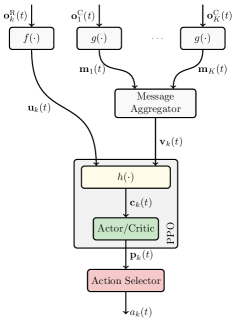
Figure 2: MEC Offloading policy network architecture.

To solve the radio resource allocation problem (1), we propose a MARL framework. Fig. 2 describes the proposed architecture, made of encoding functions $f(\cdot)$, $g(\cdot)$, and $h(\cdot)$ for features extraction, a message aggregator, an actor-critic module for policy training, and an action selector for task offloading decisions. UEs share the same policy architecture and the same parameters. However, this does not preclude UEs from taking different decisions, due to their different environment observations in the same slot. In contrast, sharing parameters limits complexity (as there is only one common policy to learn), enables efficient training, and helps to improve convergence. Inspired by our previous work [18], let $\boldsymbol{\mathrm{o}}_{k}^{\textsc{R}}(t)$ denote the set of “radio observations” of UE $k$:

$$\begin{split}\boldsymbol{\mathrm{o}}_{k}^{\textsc{R}}(t){}={}&\bigg{\{}a_{k}(t-1),R_{k,a_{k}(t-1)},R(t-1),\\ &{}\mathrm{ACK}_{k},\left\{\mathrm{RSS}_{k,n}\right\}_{n\in\mathcal{A}_{k}},\left\{\vartheta_{k,n}\right\}_{n\in\mathcal{A}_{k}}\bigg{\}}.\end{split}$$ (11)

$a_{k}(t-1)\in\mathcal{A}_{k}$ denotes UE $k$’s action (i.e., connection request to an AP) at time $t-1$, $R_{k,a_{k}(t-1)}$ is the perceived rate, $R(t-1)$ the total network sum-rate, and $\mathrm{ACK}_{k}$ the received connection acknowledgment signal. $\left\{\mathrm{RSS}_{k,n}\right\}_{n\in\mathcal{A}_{k}},\left\{\vartheta_{k,n}\right\}_{n\in\mathcal{A}_{k}}$ indicate the received signal strength and corresponding angles of arrival (AoA) from UE $k$ to AP $n$. Similarly, $\boldsymbol{\mathrm{o}}_{k}^{\textsc{C}}(t)$ represents “MEC observations”, related to task offloading:

$$\begin{split}\boldsymbol{\mathrm{o}}_{k}^{\textsc{C}}(t){}={}&\bigg{\{}(x_{k},y_{k}),f_{k}(t),Q_{k}^{l}(t),Q_{k}^{\rm s}(t),Z_{k}(t)\bigg{\}},\end{split}$$ (12)

where $Q_{k}^{l}(t)$, $Q_{k}^{\rm s}(t)$, $Z_{k}(t)$ are the queues defined above, $(x_{k},y_{k})$ are UE $k$’s geographical coordinates, and $f_{k}(t)$ its allocated CPU frequency at the ES. In our framework, after observing $\boldsymbol{\mathrm{o}}_{k}^{\textsc{R}}(t)$, UE $k$ builds its local state encoding $\boldsymbol{\mathrm{u}}_{k}$, which represents its “perception” of the radio environment, using an encoding function $f(\cdot)$, e.g., a neural network. Then, based on the aggregated MEC observations of its whole neighborhood, it constructs an encoding vector $\boldsymbol{\mathrm{v}}_{k}$, which characterizes its perception of the network from a computation viewpoint. UE $k$ then builds its overall context encoding vector $\boldsymbol{\mathrm{c}}_{k}$ to represent its global understanding of the environment, using an encoding function $h(\cdot)$, e.g., a concatenation operator or a neural network. For each UE, the goal of the MARL framework is to learn an association policy $\pi_{\boldsymbol{\mathrm{\theta}}}$ with learnable parameters $\boldsymbol{\mathrm{\theta}}$, where $\pi_{\boldsymbol{\mathrm{\theta}}}(a_{k}(t)|\boldsymbol{\mathrm{o}}_{k}(t))=p_{a_{k}(t),k}$ indicates the probability of taking action $a_{k}(t)$ after observing $\boldsymbol{\mathrm{o}}_{k}(t)=\{\boldsymbol{\mathrm{o}}_{k}^{\textsc{R}}(t),\boldsymbol{\mathrm{o}}_{k}^{\textsc{C}}(t)\}$. Note that $\boldsymbol{\mathrm{p}}_{k}(t)=[p_{0,k},\ldots,p_{N,k}]\in[0,1]^{N+1}$, from which the action $a_{k}(t)$ of the UE will be sampled, is such that $\sum_{n\in\mathcal{A}}p_{n,k}=1$ and $p_{n,k}=0$ for all $n\not\in\mathcal{A}_{k}$.

IV-A Message passing service

Let $\boldsymbol{\mathrm{W}}_{k},\boldsymbol{\mathrm{W}}_{q},\text{and~{}}\boldsymbol{\mathrm{W}}_{\nu}:\mathbb{R}^{6}\times\mathbb{R}^{m}$ be learnable weights, describing the set of parameters of the encoding function $g(\cdot)$, which we later refer to as the message generator. For each UE $l$, let $\boldsymbol{\mathrm{k}}_{l}=\boldsymbol{\mathrm{W}}_{k}^{T}\boldsymbol{\mathrm{o}}_{l}^{\textsc{C}}(t)$, $\boldsymbol{\mathrm{q}}_{l}=\boldsymbol{\mathrm{W}}_{q}^{T}\boldsymbol{\mathrm{o}}_{l}^{\textsc{C}}(t)$, $\boldsymbol{\mathrm{\nu}}_{l}=\boldsymbol{\mathrm{W}}_{\nu}^{T}\boldsymbol{\mathrm{o}}_{l}^{\textsc{C}}(t)$, and $\boldsymbol{\mathrm{m}}_{l}=\{\boldsymbol{\mathrm{q}}_{l},\boldsymbol{\mathrm{\nu}}_{l}\}$ be the key, the query, the value, and the message associated with UE $l$. Then, each UE $k$, after aggregating the messages from its neighbors $\mathcal{N}_{k}$, computes its encoding vector $\boldsymbol{\mathrm{v}}_{k}=\sum_{l\in\mathcal{N}_{k}}\alpha_{l,k}\boldsymbol{\mathrm{\nu}}_{l}$, where the score $\alpha_{l,k}$ represents the interaction between UEs $l$ and $k$ (in achieving the underlying optimization goal). This score is calculated using dot-product attention mechanism [19]: $\alpha_{l,k}=\boldsymbol{\mathrm{softmax}}\left(\left[\frac{\boldsymbol{\mathrm{q}}_{l}\boldsymbol{\mathrm{k}}_{k}^{T}}{\sqrt{m}}\right]_{l\in\mathcal{N}_{k}}\right)$. Here, $\boldsymbol{\mathrm{softmax}}(\cdot)$ denotes the normalized exponential function. Note that computing $\boldsymbol{\mathrm{v}}_{k}$ only involves the queries and the values from others UEs in $\mathcal{N}_{k}$ and not their keys, which are UE-specific and do not need to be transmitted. Such a message passing service enables the scalability and the transferability of the learned policy, which is optimized for all possible UE deployments, in sharp contrast with [10], which requires fixed UEs. In other words, in our framework, a change in the number or position of UEs in the network does not require a new policy training and does not impact the architecture of the policy network. Only the number of exchanged messages varies, depending on the variation of a UE’s neighborhood. Both, the input variables and the number of neurons of the encoding functions remain fixed. This enables curriculum learning, where a policy obtained from e.g. 6 UEs can be leveraged as a starting point to train another policy for $K>6$ UEs. Finally, all the encoding functions, including the message generator, are optimized through end-to-end proximal policy optimization (PPO) and an actor-critic framework [20].

V Numerical Results

In this section, we assess the effectiveness of the proposed framework in a network of 3 APs operating at 28-GHz mmWave frequencies and for $K\in\{6,9,12,15\}$ UEs. We use $p^{\rm u,off}=0.346$ W, $p^{\rm u,on}=0.9$ W, $p^{\rm a,off}=0.278$ W, $p^{\rm a,on}=2.2$ W, $p^{\rm s,off}=10$ W, $p^{\rm s,on}=20$ W. Each UE transmits with power $p^{\rm u,tx}(t)=\mathrm{min}\left(p_{k}^{\rm tg}(t),p_{\max}\right)$ over a bandwidth $B=10$ MHz, where $p_{k}^{\rm tg}(t)$ is the power to meet a predefined target SNR of $15$ dB and $p_{\max}=0.1$ W. Each slot lasts $10$ ms and we set $\beta=0.1$, $N_{n}=15$, $\kappa=10^{-27}$, $J_{k}=10^{-3}$, $S_{k}=1500$ bits $\forall k$ and $\mathcal{F}=\{0,0.1,\ldots,1\}\times 10^{9}\text{~{}cycle/s}$. UEs’ data generation rate follows a Poisson distribution with mean $D_{k}=50\times S_{k}$ bits $\forall k$. Additional parameters, including pathloss and antenna diagrams, can be found in [18, Table I]. In our setup, all encoding functions are composed of one multi-layer perceptron (MLPs) of $m=128$ neurons with a rectifier linear unit (ReLu) activation. Both the actor and the critic module comprise $2m$ neurons and we empirically set the learning rate to $10^{-4}$, $\epsilon_{1}=10$ and $\epsilon_{2}=0$. To foster the learned policy and enable better generalization, during training, we consider random CPU scheduling. This is possible since (1) and (1) are completely decoupled, therefore, the policy learned to solve (1) must be independent of the ES frequency allocation. We compare our solution, labeled L2OFF (Learning to Offload) in Fig. 3 and 4, to two benchmarks:

• Exhaustive search: at each slot, we perform an exhaustive search over all possible solutions of (1).

• Max-SNR: each UE is associated with a Bernoulli random variable with probability $p$ of being in active state (which models the average duty cycle of UEs). Then, at each $t$, an active UE gets associated with the AP providing the maximum signal-to-noise ratio (SNR).

All results are averaged over 200 random deployments of UEs.

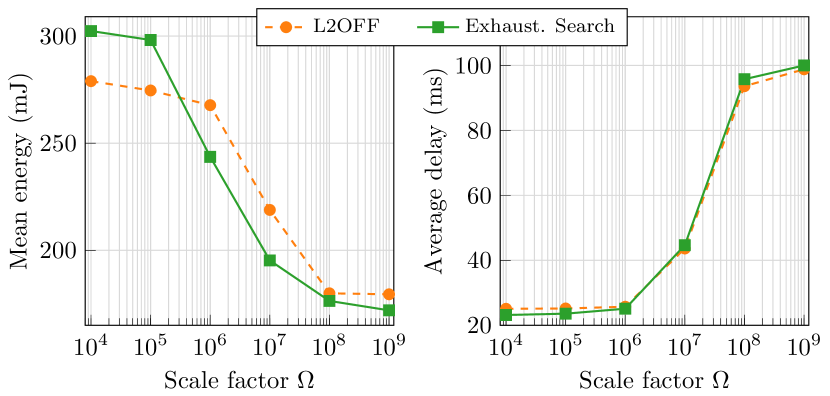
Figure 3: Energy-delay trade-off w.r.t. $\Omega$ for $K=6$ UEs and for a fixed delay constraint of $100$ ms.

Energy-delay trade-off vs. $\boldsymbol{\mathrm{\Omega}}$. Here, we evaluate the performance of our proposed framework for different values of $\Omega$ (cf. (8)), and compare the results to the performance obtained via exhaustive search in Fig. 3. First, we observe the results suggested by the theory: when $\Omega$ increases, optimally solving (1) and (1) leads to a lower energy consumption. Meanwhile, the average delay increases and caps to 100ms, which is the fixed delay constraint (C1). Interestingly, the proposed scheme exhibits performance close to exhaustive search approach (for $\Omega=10^{9}$), reaching up to $96.5\%$ of its performance, for the same delay.

Performance Comparison. To fairly compare the proposed framework with the heuristic based on Max-SNR, we first determine exhaustively the optimal lowest duty cycle that enables the Max-SNR algorithm to guarantee an average delay constraint of $100$ ms. Then, comparison is made for the same delay in Fig. 4. We can notice how, even by optimally computing the duty cycle for the Max-SNR algorithm, our solution still outperforms, reducing the energy by $10\%$ for 15 UEs compared to Max-SNR solution, as we consider interference, and intelligently orchestrate UEs. Moreover, under the same delay constraint, with our strategy, the network consumes $246$ mJ in average for $15$ UEs, whereas for the same energy consumption, the Max-SNR can only serve $12$ UEs.

VI Conclusion

In this work, we proposed a novel approach for delay constrained energy-efficient computation offloading services in dense mmWave networks impaired by interference. We first formulated the computation offloading as a long-term optimization. Then, we applied Lyapunov optimization tools to split the problem into a CPU scheduling problem and a UE-AP association problem. While the first one is easily solvable via an efficient iterative algorithm, we solved the second one thanks to multi-agent reinforcement learning with a distributed and transferable policy. The proposed solution reaches up to $96.5\%$ of the optimal solution obtained via exhaustive search and can reduce energy consumption up to $10\%$ compared to a heuristic approach based on SNR maximization.

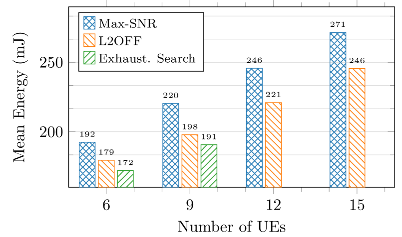
Figure 4: Average energy for a fixed average delay of $100$ ms. Due to complexity, results for $K\in\{12,15\}$ UEs cannot be obtained for the exhaustive search.

References

- [1] E. Calvanese Strinati et al., “6G: The Next Frontier: From Holographic Messaging to Artificial Intelligence Using Subterahertz and Visible Light Communication,” IEEE Vehicular Technology Magazine, vol. 14, no. 3, pp. 42–50, 9 2019.
- [2] S. Ahmadi, 5G NR: Architecture, Technology, Implementation, and Operation of 3GPP New Radio Standards. Elsevier Science, 2019.
- [3] Q. Pham et al., “A Survey of Multi-Access Edge Computing in 5G and Beyond: Fundamentals, Technology Integration, and State-of-the-Art,” IEEE Access, vol. 8, pp. 116 974–117 017, 2020.
- [4] L. Li, Q. Guan, L. Jin, and M. Guo, “Resource Allocation and Task Offloading for Heterogeneous Real-Time Tasks With Uncertain Duration Time in a Fog Queueing System,” IEEE Access, vol. 7, pp. 9912–9925, 2019.
- [5] L. Chen, S. Zhou, and J. Xu, “Energy Efficient Mobile Edge Computing in Dense Cellular Networks,” in IEEE ICC, 2017, pp. 1–6.
- [6] S. Wang, X. Zhang, Z. Yan, and W. Wang, “Cooperative Edge Computing with Sleep Control under Non-uniform Traffic in Mobile Edge Networks,” IEEE Internet Things J., 10 2018.
- [7] P. Chang and G. Miao, “Resource Provision for Energy-Efficient Mobile Edge Computing Systems,” in 2018 IEEE GLOBECOM, 2018, pp. 1–6.
- [8] Y. Nan, W. Li, W. Bao, F. C. Delicato, P. F. Pires, Y. Dou, and A. Y. Zomaya, “Adaptive Energy-Aware Computation Offloading for Cloud of Things Systems,” IEEE Access, vol. 5, pp. 23 947–23 957, 2017.
- [9] B. Yu, L. Pu, Q. Xie, J. Xu, and J. Zhang, “U-MEC: Energy-Efficient Mobile Edge Computing for IoT Applications in Ultra Dense Networks,” in Wireless Algorithms, Systems, and Applications, 2018, pp. 622–634.
- [10] S. Bi, L. Huang, H. Wang, and Y. A. Zhang, “Lyapunov-guided Deep Reinforcement Learning for Stable Online Computation Offloading in Mobile-Edge Computing Networks,” Available online: https://arxiv.org/abs/2010.01370, 2020.
- [11] S. Bae, S. Han, and Y. Sung, “A Reinforcement Learning Formulation of the Lyapunov Optimization: Application to Edge Computing Systems with Queue Stability,” Available online: https://arxiv.org/abs/2012.07279, 2020.
- [12] M. Merluzzi, P. Di Lorenzo, S. Barbarossa, and V. Frascolla, “Dynamic Computation Offloading in Multi-Access Edge Computing via Ultra-Reliable and Low-Latency Communications,” IEEE Transactions on Signal and Information Processing over Networks, pp. 1–1, 2020.
- [13] J. D. C. Little, “A proof for the queuing formula: ,” Oper. Res., vol. 9, no. 3, p. 383–387, Jun. 1961.
- [14] E. Le Sueur and G. Heiser, “Dynamic Voltage and Frequency Scaling: The Laws of Diminishing Returns,” in Proc. HotPower, 2010, pp. 1–8.
- [15] T. D. Burd and R. W. Brodersen, “Processor design for portable systems,” J. VLSI Signal Process. Syst., vol. 13, no. 2-3, pp. 203–221, 8 1996.
- [16] M. Merluzzi, N. di Pietro, P. Di Lorenzo, E. Calvanese Strinati, and S. Barbarossa, “D-MEC: Discontinuous Mobile Edge Computing,” Available online: https://arxiv.org/pdf/2008.03508.pdf, 8 2020.
- [17] M. J. Neely, Stochastic Network Optimization with Application to Communication and Queueing Systems. Morgan & Claypool Publishers, 2010.
- [18] M. Sana, A. De Domenico, W. Yu, Y. Lostanlen, and E. Calvanese Strinati, “Multi-Agent Reinforcement Learning for Adaptive User Association in Dynamic mmWave Networks,” IEEE Transactions on Wireless Communications, vol. 19, no. 10, pp. 6520–6534, 2020.
- [19] A. Vaswani, N. Shazeer, N. Parmar, J. Uszkoreit, L. Jones, A. N. Gomez, Ł. Kaiser, and I. Polosukhin, “Attention is all you need,” in Advances in neural information processing systems, 2017, pp. 5998–6008.
- [20] J. Schulman, F. Wolski, P. Dhariwal, A. Radford, and O. Klimov, “Proximal Policy Optimization Algorithms.” CoRR, vol. abs/1707.06347, 2017.