Learning Lipschitz Feedback Policies from Expert Demonstrations: Closed-Loop Guarantees, Generalization and Robustness

Abstract

In this work, we propose a framework to learn feedback control policies with guarantees on closed-loop generalization and adversarial robustness. These policies are learned directly from expert demonstrations, contained in a dataset of state-control input pairs, without any prior knowledge of the task and system model. We use a Lipschitz-constrained loss minimization scheme to learn feedback policies with certified closed-loop robustness, wherein the Lipschitz constraint serves as a mechanism to tune the generalization performance and robustness to adversarial disturbances. Our analysis exploits the Lipschitz property to obtain closed-loop guarantees on generalization and robustness of the learned policies. In particular, we derive a finite sample bound on the policy learning error and establish robust closed-loop stability under the learned control policy. We also derive bounds on the closed-loop regret with respect to the expert policy and the deterioration of closed-loop performance under bounded (adversarial) disturbances to the state measurements. Numerical results validate our analysis and demonstrate the effectiveness of our robust feedback policy learning framework. Finally, our results suggest the existence of a potential tradeoff between nominal closed-loop performance and adversarial robustness, and that improvements in nominal closed-loop performance can only be made at the expense of robustness to adversarial perturbations.

I Introduction

Robustness of data-driven models to adversarial perturbations has attracted much attention in recent years. One of the approaches to robust learning seeks to modulate the Lipschitz constant of the data-driven model [1, 2, 3], either via a regularization [4, 5] of the learning loss function or by imposing a Lipschitz constraint [6, 7]. Since the Lipschitz constant determines the (worst-case) sensitivity of a model to perturbations of the input, data-driven models trained with Lipschitz constraints/regularizers are expected to be robust to bounded (adversarial) perturbations [8]. Prior works have primarily explored this approach for static input-output models [7, 8, 9]. However, in a feedback control setting, a static input-output robustness guarantee for a data-driven controller may not result in robust closed-loop performance. When a data-driven controller is integrated into the feedback loop, a static input-output robustness guarantee for the data-driven controller must be combined with appropriate robust control notions to yield a robustness certificate for the closed-loop system [10, 11]. Obtaining safety and robustness certificates for data-driven controllers in closed-loop systems remains an active area of research in general. In this work, we propose a learning framework to learn Lipschitz feedback policies with provable guarantees on closed-loop performance and robustness against bounded adversarial perturbation, where these policies are learned directly from expert demonstrations without any prior knowledge of the task and the system model.

The problem of learning optimal feedback control policies from data for a nonlinear system with unknown dynamics and control cost is not only technically challenging, but also has high sample complexity, which presents obstacles for data collection and the use of data-driven algorithms. In imitation learning framework, this issue is often mitigated by expert demonstrations of the optimal feedback policy, which help reduce the problem to one of learning the policy implemented by the expert. Yet, learning is not a simple repetition of the expert controls, but rather the ability to generalize and respond to unseen conditions as the expert demonstrator would. A naive learning approach (such as behavioral cloning in imitation learning [12]) that overlooks the generalization and robustness requirements may not only result in pointwise differences between the expert and implemented policies, but also in unstable trajectories and failure of the controlled system [13]. This raises the following question: For an unknown system and control task, what is an appropriate method to learn a feedback policy from a finite number of expert demonstrations (dataset of state-control input pairs) such that (i) the learned policy generalizes expert performance beyond the finite data points to a broader region of interest, and (ii) closed-loop performance remains robust to (adversarial) disturbances of the state measurements.

Related work. There have been several proposals to address the above question in various settings. Broadly, this problem falls under the umbrella of imitation learning, which has been studied extensively in the literature and implemented in various contexts including video games [13, 14], robotics [15] and autonomous driving [16].
Generalization: The key obstacle to widespread adoption of imitation learning is that it is difficult to guarantee performance in unseen scenarios. One approach to overcome this obstacle is inverse reinforcement learning (also referred to as apprenticeship learning in the literature), where the learner infer the unknown cost function from expert demonstrations, then learn an optimal policy that optimizes the learned cost using reinforcement learning [17, 18, 19, 20, 21]. Since the learned cost represents the task of the expert, inverse reinforcement learning algorithms are able to generalize to unseen scenarios that are not covered by the expert demonstrations. However, one drawback of inverse reinforcement learning is that there can exist multiple cost functions that can be optimized under the expert’s policy, which adds ambiguity in learning the cost function [22]. Another approach that overcomes the obstacle of performing in unseen scenarios is direct policy learning via interactive expert [13, 23]. In this approach, the learner can query an interactive expert at each iteration, then, the learner uses the expert’s feedback to correct its mistakes and improve its policy. Since this approach keeps expanding the expert’s data, it will eventually cover all possible scenarios in the long run. However, one drawback of this approach is that it requires the expert to be always available for feedback. In [24], noise is injected into the expert’s policy in order to provide demonstrations on how to recover from errors. In [25], the authors develop a framework for learning a generative model for planning trajectories from demonstrations, which allows it to capture uncertainty about previously unseen scenarios.
Closed-loop performance and robustness: Several approaches to adversarial imitation learning have been proposed in [26, 27], where inverse reinforcement learning is used. In [28], the authors proposed an adversarially robust imitation learning framework, where an agent is trained in an adversarially perturbed environment with the expert being available for queries at any time step. In [29], the authors learn robust control barrier functions from safe expert demonstrations. In all these works, robustness of imitation learning algorithms is considered to be the ability of the learned policy to recover from errors, which is similar to the notion of generalization.

In contrast to many of the works referenced above, we seek a principled feedback policy learning framework with strong theoretical guarantees. In particular, we seek explicit bounds on the finite sample performance, stability and robustness of the closed-loop system under the learned feedback policy. The broader problem of obtaining closed-loop performance and robustness guarantees for learned feedback policies and understanding the underlying tradeoffs has attracted attention recently [30, 31, 32]; yet it remains an active area of research. This requires the integration of theoretical tools from several areas: (i) the underlying control task is typically specified as an optimal control problem with performance measured in terms of the cost incurred, (ii) the feedback control policy is learned from finite offline data which involves considerations of generalization and robustness to distributional shifts, and (iii) closed-loop performance guarantees typically rely on an underlying robust stability guarantee for the learned policy. Prior works have addressed this problem within various frameworks, such as the $H_{\infty}$-control framework for linear systems [33]. However, the problem of obtaining guarantees on closed-loop generalization and robustness to distributional shifts of learned policies for general nonlinear systems still remains a challenge. In this work, we address this problem within a Lipschitz feedback policy learning framework. The Lipschitz property is a fairly mild requirement in nonlinear control, and through our analysis we will see that it can be exploited to provide closed-loop bounds on generalization and robustness to distributional shifts for learned policies, highlighting the effectiveness of this approach.

Contributions. Our primary contribution in this paper is a robust feedback control policy learning framework based on Lipschitz-constrained loss minimization, where the feedback policies are learned directly from expert demonstrations. We then undertake a systematic study of the performance of feedback policies learned within our framework using meaningful metrics to measure closed-loop stability, performance and robustness. Our work integrates robust learning, optimal control and robust stability into a unified framework for robust feedback policy learning. More specifically, our technical contributions include: (i) an analysis of the Lipschitz-constrained policy learning problem, resulting in a finite sample bound on the learning error, (ii) a robust stability bound for the closed-loop system under the learned feedback policies, (iii) a Lipschitz analysis resulting in a bound on the regret incurred by learned feedback policies in terms of the learning error, and a bound on the deterioration of performance in the presence of (adversarial) disturbances to state measurements. This sheds light on the dependence of closed-loop control performance and robustness on learning. Conversely, our results specify target bounds on policy learning error for desired closed-loop performance. We then demonstrate our robust feedback policy learning framework via numerical experiments on (i) the standard LQR benchmark, and (ii) a non-holonomic differential drive mobile robot model. Finally, our analysis points to the existence of a potential tradeoff between nominal performance of the learned policies and their robustness to adversarial disturbances of the feedback, which is borne out in numerical experiments where we observe that improvements to adversarial robustness can only be made at the expense of nominal performance.

Notation. For open and bounded sets $\mathcal{X}\subset\mathbb{R}^{{\rm dim}(\mathcal{X})}$ and $\mathcal{Y}\subset\mathbb{R}^{{\rm dim}(\mathcal{Y})}$, and a Lipschitz continuous map $f:\mathcal{X}\rightarrow\mathcal{Y}$, we denote by $\ell_{f}$ the Lipschitz constant of $f$. Furthermore, we denote by $\mathrm{Lip}(\mathcal{X};\mathcal{Y})$ the space of Lipschitz continuous maps from $\mathcal{X}$ to $\mathcal{Y}$. We denote by $\mathrm{Vol}(\mathcal{X})$ the volume of $\mathcal{X}$. A function $g:\mathcal{X}\rightarrow\mathbb{R}$ is said to be $\lambda$-smooth if it has a Lipschitz-continuous gradient, i.e., $\left\|\nabla g(x_{1})-\nabla g(x_{2})\right\|\leq\lambda\left\|x_{1}-x_{2}\right\|$ for any $x_{1},x_{2}\in\mathcal{X}$, where $\|\cdot\|$ denotes the norm operator. A continously differentiable function $g:\mathcal{X}\rightarrow\mathbb{R}$ is said to be $\mu$-strongly convex if $\left\|\nabla g(x_{1})-\nabla g(x_{2})\right\|\geq\mu\left\|x_{1}-x_{2}\right\|$ for any $x_{1},x_{2}\in\mathcal{X}$. The maximum eigenvalue of a square matrix $A$ is denoted by $\rho(A)$. The cardinality of a set $\mathcal{X}$ is denoted by $|\mathcal{X}|$.

II Problem formulation and outline of the approach

In the section, we setup the problem of learning robust feedback control policies from expert demonstrations and present an outline of our approach.

II-A Problem setup

We begin by specifying the properties of the system, the control task and the dataset of expert demonstrations. Consider a discrete-time nonlinear system of the form:

$$\begin{aligned} x_{t+1}=f(x_{t},u_{t}),\qquad y_{t}=x_{t}+\delta_{t},\end{aligned}$$ (1)

where the map $f:\mathbb{R}^{n}\times\mathbb{R}^{m}\rightarrow\mathbb{R}^{n}$ denotes the dynamics, $x_{t}\in\mathbb{R}^{n}$ the state, $u_{t}\in\mathbb{R}^{m}$ the control input and $y_{t}\in\mathbb{R}^{n}$ the full-state measurement at time $t\in\mathbb{N}$, respectively, with disturbance $\|\delta_{t}\|\leq\zeta$ for any $t\in\mathbb{N}$.

Assumption II.1 (System properties).

The following properties hold for System (1):

1. Fixed point at origin: The map $f$ in (1) has a fixed point at the origin (i.e., $f(0,0)=0$).

2. Lipschitz continuous dynamics: The map $f$ in (1) is Lipschitz continuous with constants $\ell_{f}^{x}$ and $\ell_{f}^{u}$ (i.e., $\left\|f(x_{1},u_{1})-f(x_{2},u_{2})\right\|\leq\ell_{f}^{x}\|x_{1}-x_{2}\|+\ell_{f}^{u}\|u_{1}-u_{2}\|$ for any $x_{1},x_{2}\in\mathbb{R}^{n}$ and $u_{1},u_{2}\in\mathbb{R}^{m}$).

3. Exponential stabilizability by Lipschitz feedback: System (1) is uniformly exponentially stabilizable by Lipschitz feedback, i.e., there exists a Lipschitz continuous feedback policy $\pi$ and constants $M\in\mathbb{R}_{\geq 0}$, $\beta\in(0,1)$ such that $\left\|f_{\pi}^{t}(x)\right\|\leq M\beta^{t}\|x\|$. $\square$

We now explain the motivation behind the above assumptions on the properties of System (1). The control task is often formulated as one of stabilizing the system to the origin. Assumption II.1-(i) states that the origin, in the absence of control input, is indeed a fixed point of the system. The Lipschitz continuity Assumption II.1-(ii) specifies the level of regularity intrinsic to the system dynamics and is fairly standard in the literature. From a control design perspective it is crucial that the system indeed possesses the desired stabilizability properties from within this class of feedback policies considered in design. In this paper, we seek to learn feedback policies with Lipschitz regularity and Assumption II.1 specifies that this is the case and that System (1) is exponentially stabilizable by Lipschitz feedback.

The task is one of infinite-horizon discounted optimal control of System (1) by a Lipschitz-continuous feedback policy, with stage cost $c:\mathbb{R}^{n}\times\mathbb{R}^{m}\rightarrow\mathbb{R}_{\geq 0}$ and discount factor $\gamma\in(0,1)$:

$$\begin{aligned} &\min_{\pi\in\mathrm{Lip}(\mathbb{R}^{n};\mathbb{R}^{m})}~{}\sum_{t=0}^{\infty}\gamma^{t}c(x_{t},u_{t}),\\ &\qquad\;~{}\text{s.t.}~{}\begin{cases}x_{t+1}&=f(x_{t},u_{t}),\\ u_{t}&=\pi(x_{t}+\delta_{t}),\end{cases}\end{aligned}$$ (2)

where $\mathrm{Lip}(\mathbb{R}^{n};\mathbb{R}^{m})$ is the space of Lipschitz-continuous feedback policies. Furthermore, we would like the closed-loop performance to be robust to the disturbance $\delta$.

Assumption II.2 (Task properties).

The following hold for Task (2) and System (1):

1. Strong convexity and smoothness of stage cost: The stage cost $c:\mathbb{R}^{n}\times\mathbb{R}^{m}\rightarrow\mathbb{R}_{\geq 0}$ is $\mu$-strongly convex and $\lambda$-smooth. Furthermore, $c(x,u)=0$ if and only if $x=0$ and $u=0$.

2. Existence of optimal feedback policy: For every $\gamma\in(0,1)$, there exists a minimizer $\pi^{*}\in\mathrm{Lip}(\mathbb{R}^{n};\mathbb{R}^{m})$ to the optimal control problem (2) with $\delta\equiv 0$. $\square$

The choice of optimal control cost function plays an important role in determining the properties of the optimal feedback policy. Assumption II.2-(i) specifies the convexity and smoothness properties of the control cost. Existence of an optimal feedback policy within the considered class, as specified in Assumption II.2-(ii) is a minimum requirement for control design.

We now verify the properties in Assumptions II.1 and II.2 in the Linear-Quadratic control setting.

Example 1 (Linear quadratic control).

For a linear system with $f(x,u)=Ax+Bu$ such that $(A,B)$ is a controllable pair, it can be seen that the properties in Assumption II.1 readily follow. It can be seen that a quadratic stage cost $c(x,u)=x^{\top}Qx+2x^{\top}Wu+u^{\top}Ru$ (with $Q>0$ and $R-W^{\top}Q^{-1}W>0$) is strongly convex and has a Lipschitz-continuous gradient with $\mu=\lambda_{\min}(H)$, $\lambda=\lambda_{\max}(H)$, and $H=2\left[\begin{matrix}Q&W\\ W^{\top}&R\end{matrix}\right]$, thereby satisfying Assumption II.2-(i). Furthermore, we note that Assumption II.2-(ii) readily follows from the existence of an optimal feedback gain for the discounted infinite-horizon LQR problem, and the fact that the corresponding optimal value function is quadratic.

In this paper, we consider the problem of data-driven feedback control, where we have access neither to the underlying dynamics $f$ nor to the task cost function (stage cost $c$ and discount factor $\gamma$). Instead, we have access to $N<\infty$ expert demonstrations of an (unknown) optimal feedback policy $\pi^{*}$ on System (1) over a finite horizon of length $T$. The initial state of the demonstrations is sampled uniformly i.i.d. from $B_{r}(0)\subset\mathbb{R}^{n}$, the ball of radius $r$ centered at the origin. The data is collected in the form of matrices $X,U$ as follows:

$$X=\left[\begin{matrix}\mathbf{x}^{(1)}&\ldots&\mathbf{x}^{(N)}\end{matrix}\right],\quad U=\left[\begin{matrix}\mathbf{u}^{(1)}&\ldots&\mathbf{u}^{(N)}\end{matrix}\right],$$

where $\mathbf{x}^{(i)}=(x_{0}^{(i)},\ldots,x_{T}^{(i)})$ and $\mathbf{u}^{(i)}=(u_{0}^{(i)},\ldots,u_{T-1}^{(i)})$ are the state and input vectors from the $i$-th demonstration, satisfying $u_{t}^{(i)}=\pi^{*}(x_{t}^{(i)})$ for all $i\in\{1,\ldots,N\}$ and $t\in\{0,\ldots,T-1\}$.

II-B Outline of the approach

Our objective is to learn a feedback policy from the dataset $X,U$ of expert demonstrations to solve the control task (2) while remaining robust to (adversarial) disturbances $\delta$ of full-state measurements. To this end, we seek an optimization-based learning formulation that allows us to explicitly constrain the sensitivity of the learned policy to (adversarial) disturbances. The Lipschitz constant of the learned policy serves as a measure of its sensitivity to disturbances, and we thereby formulate the (adversarially) robust policy learning problem as a Lipschitz-constrained policy learning problem [7]:

$$\begin{aligned} &\underset{\pi\in\mathrm{Lip}(B_{r}(0);\mathbb{R}^{m})}{\min}\quad\frac{1}{NT}\sum_{i=1}^{N}\sum_{t=0}^{T-1}L\left(\pi(x_{t}^{(i)}),u_{t}^{(i)}\right),\\ &\qquad\quad\text{s.t.}\qquad\quad\;\mathrm{lip}(\pi)\leq\alpha,\end{aligned}$$ (3)

where $L$ is a strictly convex and Lipschitz continuous loss function for the learning problem, $\mathrm{lip}(\pi)$ is the Lipschitz constant of the policy $\pi$, and $\alpha\in\mathbb{R}_{\geq 0}$ is a target upper bound for the Lipschitz constant of the learned policy $\widehat{\pi}$ (the minimizer in (3)). The Lipschitz constraint in (3) serves as a mechanism to induce robustness of the learned policy to disturbances $\delta$ (the smaller the parameter $\alpha$, the more robust the policy $\widehat{\pi}$ is to the disturbances $\delta$ [1]). Figure 1 illustrates our setup.

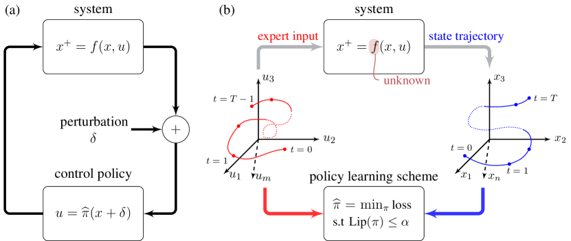
Figure 1: The block diagram in panel (a) corresponds to the implementation of the learned control policy $\widehat{\pi}$ in non-nominal conditions under adversarial perturbations $\delta$ on the state measurement. Panel (b) illustrates the Lipschitz-constrained policy learning scheme implemented on the expert generated dataset to obtain policy $\widehat{\pi}$.

We then use the robustness of the learned policy, along with a bound on the training loss, to obtain guarantees on the closed-loop performance under the learned policy $\widehat{\pi}$. For this, we first combine the training loss with the Lipschitz bound to obtain a bound on the worst-case error $\left\|\widehat{\pi}-\pi^{*}\right\|_{\infty}$, where $\left\|\widehat{\pi}-\pi^{*}\right\|_{\infty}=\sup_{x\in B_{r}(0)}\left\|\widehat{\pi}(x)-\pi^{*}(x)\right\|$. Then for a given worst-case learning error bound $\left\|\widehat{\pi}-\pi^{*}\right\|_{\infty}\leq\varepsilon$, we obtain via our analysis (i) a robust closed-loop stability bound as a function of $\varepsilon$, and (ii) bounds on closed-loop performance (measured in terms of the cost (16) incurred on the task) as a function of $\varepsilon$. Conversely, in order to satisfy target bounds on stability and performance, our analysis can be used to obtain a target bound on $\varepsilon$ which must be satisfied by the learned policy, if some additional information on the system and task are available.

We now develop appropriate notions of closed-loop performance and robustness under the feedback policies learned from expert demonstrations. We note that the control task (2), being one of optimal control of System (1), has a natural performance metric given by the value function. Let $V^{\widehat{\pi}}$ be the value function associated with the learned feedback policy $\widehat{\pi}$ for System (1):

$$\begin{aligned} V^{\widehat{\pi}}(x)=\sum_{t=0}^{\infty}\gamma^{t}c_{\pi}\left(f_{{\widehat{\pi}}}^{t}(x)\right).\end{aligned}$$ (4)

Since the expert implements the optimal policy $\pi^{*}$, the performance of the learned policy can be measured by its regret with respect to the expert policy $\pi^{*}$. The regret associated with the learned policy $\widehat{\pi}$ relative to the expert policy $\pi^{*}$ is:

$${\mathcal{R}}(\widehat{\pi})=\sup_{x\in B_{r}(0)}\left\{V^{\widehat{\pi}}(x)-V^{*}(x)\right\}.$$ (5)

When $\mathcal{R}(\widehat{\pi})=0$, the performance of the learned policy equals the performance of an optimal policy for the control task (2). Conversely, the performance of the learned policy degrades as $\mathcal{R}(\widehat{\pi})$ increases. Naturally, the objective of the policy learning problem is now to minimize the regret incurred by the learned policy $\widehat{\pi}$. Note that this is a more important performance metric in the closed-loop setting than the loss function $L$ used for learning in (3), as it encodes the cost incurred by the evolution of the system under the learned feedback policy. We now note that the regret $\mathcal{R}$ only measures the performance of the learned policy under nominal conditions (in the absence of perturbations on the state measurements) and does not shed light on its performance in the presence of adversarial perturbations. This calls for an appropriate robustness metric, for which we will use the regret associated with the policy $\widehat{\pi}$ when subject to perturbations relative to when deployed under nominal conditions, that is,

$${\mathcal{S}}(\widehat{\pi})=\sup_{x\in B_{r}(0)}\left\{V^{\widehat{\pi}_{\delta}}(x)-V^{\widehat{\pi}}(x)\right\},$$ (6)

where $\widehat{\pi}_{\delta}(x)=\widehat{\pi}(x+\delta)$. Intuitively, if ${\mathcal{S}}(\widehat{\pi})$ is small, then the performance of the policy $\widehat{\pi}$ under perturbation is close to its performance in nominal conditions, and $\widehat{\pi}$ is robust to feedback perturbations. Again, we note that this robustness metric measures closed-loop robustness by encoding the cost incurred by the evolution of the system under the learned feedback policy subject to feedback perturbations. We would ideally like to keep both $\mathcal{R}$ and $\mathcal{S}$ low, which would imply that the policy performs well both under nominal conditions and when subjected to feedback perturbations. However, we shall see later that there may exist tradeoffs between the two objectives, presenting an obstacle to such a goal.

We now address some crucial technical issues arising in the closed-loop dynamic setting in relation to minimizing the performance metrics $\mathcal{R}$ and $\mathcal{S}$. We note that the policy learning problem (3) is formulated over the set $B_{r}(0)\in\mathbb{R}^{n}$, which is the region of interest containing the data from expert demonstrations. Now, in order to measure the performance of a learned policy $\widehat{\pi}$ using the metrics $\mathcal{R}$ and $\mathcal{S}$, we must first ensure that the closed-loop trajectories of the system, under policy $\widehat{\pi}$, remain in $B_{r}(0)$ (for initial conditions in $B_{r}(0)$). In the absence of such a guarantee, the metrics $\mathcal{R}$ and $\mathcal{S}$ are likely to be unbounded, and would therefore not serve as useful measures of performance. We therefore obtain robust stability bounds that specify the conditions under which closed-loop trajectories remain bounded in $B_{r}(0)$.

III Robust closed-loop stability and performance

In this section, we present the theoretical results underlying the robust feedback policy learning framework outlined in Section II. The results are presented in three parts: (i) We begin with an analysis of the Lipschitz-constrained policy learning problem (3). In Theorem IV.1, we provide a finite sample guarantee on the maximum learning error incurred in the region of interest $B_{r}(0)$, i.e., $\left\|\widehat{\pi}-\pi^{*}\right\|_{\infty}$. This guarantee on the learning error bound is to be combined with the closed-loop stability and performance guarantees obtained later for policies satisfying a given learning error bound. (ii) We then present a closed-loop stability analysis for System (1) under learned feedback control policies satisfying a given learning error bound. In Theorem III.3-(i) we establish that the closed-loop system under optimal feedback $\pi^{*}$ is exponentially stable. Furthermore, in Theorem III.3-(ii) we establish a robust stability guarantee (to bounded adversarial disturbances on the state measurements) for learned feedback control policies satisfying a given learning error bound. (iii) We finally present an analysis of performance on the control task (LABEL:eq:_nonlinear_control_task) under learned feedback control policies satisfying a given learning error bound. Theorem III.6-(i) provides an upper bound on the regret incurred by the learned policy with respect to the expert policy. Theorem III.6-(ii) quantifies the robustness of the closed-loop performance in terms of the Lipschitz constant of the learned feedback policy.

III-A Robust stability with learned feedback policy

We first present the following result on the quadratic boundedness of the optimal value function:

Lemma III.1 (Quadratic boundedness of optimal value function).

There exist $\underline{\kappa}^{*},\bar{\kappa}^{*}\in\mathbb{R}_{\geq 0}$ such that $\frac{\mu}{2}\leq\underline{\kappa}^{*}\leq\bar{\kappa}^{*}$ and the optimal value function in (2) satisfies $\underline{\kappa}^{*}\|x\|^{2}\leq V^{*}(x)\leq\bar{\kappa}^{*}\|x\|^{2}$.

We make the following assumption on the constants $\underline{\kappa}^{*},\bar{\kappa}^{*}$ in Lemma III.1:

Assumption III.2 (Bounds on $\underline{\kappa}^{*},\bar{\kappa}^{*}$).

For $\gamma\in\left(1-\mu/\left(\lambda\sqrt{1+{\alpha^{*}}^{2}}\right),1\right)$, the constants $\underline{\kappa}^{*},\bar{\kappa}^{*}$ in Lemma III.1 are such that $\lambda\sqrt{1+{\alpha^{*}}^{2}}/2\leq\underline{\kappa}^{*}\leq\bar{\kappa}^{*}<\underline{\kappa}^{*}+\mu/2$.

The following theorem establishes robust stability of the closed-loop system under the learned policy $\widehat{\pi}$ from a bound on the policy error $\left\|\widehat{\pi}(x)-\pi^{*}(x)\right\|_{\infty}$ and measurement disturbances $\delta$:

Theorem III.3 (Robust exponential stability under Lipschitz policy).

Let $\gamma^{\prime}=1-\mu/(2\bar{\kappa}^{*})$. Let $\pi^{*}$ be the minimizer in (2) for some $\gamma\in\left(\bar{\kappa}^{*}\gamma^{\prime}/\underline{\kappa}^{*}\;,\;1\right)$, and let $\widehat{\pi}$ be any policy such that $\left\|\widehat{\pi}-\pi^{*}\right\|_{\infty}\leq\varepsilon$ and $\mathrm{lip}\left(\widehat{\pi}\right)\leq\alpha$. Let $\alpha\zeta+\varepsilon\leq\frac{1}{\ell_{f}^{u}}\left(1-\sqrt{\frac{\bar{\kappa}^{*}\gamma^{\prime}}{\underline{\kappa}^{*}\gamma}}\right)r$ and let $\left\|\delta_{t}\right\|\leq\zeta$ for all $t\in\mathbb{N}$. For the closed-loop trajectory $f_{\widehat{\pi}_{\delta}}^{t}(x)$ starting from $x\in B_{r}(0)$ and generated by the policy $\widehat{\pi}_{\delta}$, the following holds:

$$\small\begin{aligned} &\left\|f_{\widehat{\pi}_{\delta}}^{t}(x)-f_{\pi^{*}}^{t}(x)\right\|\\ &\leq\min\left\{\Delta_{t},~{}2\left[\frac{\bar{\kappa}^{*}\gamma^{\prime}}{\underline{\kappa}^{*}\gamma}\right]^{\frac{t}{2}}\|x\|+\ell_{f}^{u}\left[\frac{1-\left[\frac{\bar{\kappa}^{*}\gamma^{\prime}}{\underline{\kappa}^{*}\gamma}\right]^{\frac{t}{2}}}{1-\left[\frac{\bar{\kappa}^{*}\gamma^{\prime}}{\underline{\kappa}^{*}\gamma}\right]^{\frac{1}{2}}}\right](\alpha\zeta+\varepsilon),~{}2r\right\}\end{aligned}$$

where $\Delta_{t}=\begin{cases}\left[\frac{1-\ell_{f_{\pi^{*}}}^{t}}{1-\ell_{f_{\pi^{*}}}}\right]\cdot\ell_{f}^{u}(\alpha\zeta+\varepsilon),\quad~{}&\text{if}~{}\ell_{f_{\pi^{*}}}\neq 1,\\ \vskip 3.0pt plus 1.0pt minus 1.0ptt\cdot\ell_{f}^{u}(\alpha\zeta+\varepsilon),\quad~{}&\text{if}~{}\ell_{f_{\pi^{*}}}=1.\end{cases}$

We refer the reader to Appendix A-B for the proof. The robust stability result can be understood in the sense of input-to-state stability [35, 36], in that we exploit the exponential stability result for the expert policy $\pi^{*}$ and treat the learned policy $\widehat{\pi}$ as a perturbation on $\pi^{*}$. By obtaining boundedness of the learning error along the closed-loop trajectory, we establish that the closed-loop trajectory under the learned policy both stays within a bounded region around the optimal trajectory and converges asymptotically to a bounded region around the origin.

III-B Regret and robustness with learned feedback policy

Having clarified the issue of robust stability, we now present a regret analysis for the learned control policy $\widehat{\pi}$. We first present the following lemma on an incremental exponential stability property of exponentially stabilizing Lipschitz feedback policies on $B_{r}(0)$:

Lemma III.4 (Incremental exponential stability).

Let $\pi$ be an exponentially stabilizing Lipschitz feedback policy for System (1) such that $\left\|f_{\pi}^{t}(x)\right\|\leq M\beta^{t}\|x\|$ for some $M\in\mathbb{R}_{\geq 0}$ and $\beta\in(0,1)$ and $B_{r}(0)$ is $f_{\pi}$-invariant. For $x,x^{\prime}\in B_{r}(0)$, there exists $M(x_{1},x_{2})\in\mathbb{R}_{\geq 0}$ such that $\left\|f_{\pi}^{t}(x)-f_{\pi}^{t}(x^{\prime})\right\|\leq M(x_{1},x_{2})\beta^{t}\|x_{1}-x_{2}\|$.

We make the following assumption on the existence of a uniform bound on $M(x_{1},x_{2})$ in Lemma III.4 over $x_{1},x_{2}\in B_{r}(0)$:

Assumption III.5 (Uniform incremental exponential stability).

The optimal policy $\pi^{*}$ in (2) is such that for any $\pi\in\mathrm{Lip}(B_{r}(0);\mathbb{R}^{m})$ satisfying $\left\|\pi-\pi^{*}\right\|_{\infty}\leq\left(1-\sqrt{\bar{\kappa}^{*}\gamma^{\prime}/(\underline{\kappa}^{*}\gamma)}\right)r/\ell_{f}^{u}$, there exists a constant $M=\sup_{x_{1},x_{2}\in B_{r}(0)}M(x_{1},x_{2})$ in Lemma III.4.

The following theorem establishes a bound on the sub-optimality of the closed-loop performance of system (1) with $\widehat{\pi}$ and a robustness bound for the deterioration of the closed-loop performance under bounded disturbances:

Theorem III.6 (Regret and robustness of learned policy).

Let $\gamma^{\prime}$ be as specified in Theorem III.3, $M,\beta$ be as in Lemma III.4 and Assumption III.5, and let $\pi^{*}$ be the minimizer in (2) for some $\gamma\in\left(\bar{\kappa}^{*}\gamma^{\prime}/\underline{\kappa}^{*}\;,\;1\right)$. Let $\varepsilon\leq\left(1-\sqrt{\bar{\kappa}^{*}\gamma^{\prime}/(\underline{\kappa}^{*}\gamma)}\right)r/\ell_{f}^{u}$, $\widehat{\pi}$ be any policy such that $\left\|\widehat{\pi}-\pi^{*}\right\|_{\infty}\leq\varepsilon$ and $\mathrm{lip}\left(\widehat{\pi}\right)\leq\alpha$. Furthermore, let $\Theta=M^{2}/(1-\gamma\beta^{2})$.

(i) Regret: The regret $\mathcal{R}$ of the policy $\widehat{\pi}$ relative to $\pi^{*}$, as defined in (5), satisfies:

$${\mathcal{R}}(\widehat{\pi})\leq\frac{\lambda}{1-\gamma}\left[c_{1}r\sqrt{1+\left|\max\left\{\alpha,\alpha^{*}\right\}\right|^{2}}~{}\Delta+\frac{1}{2}c_{2}\Delta^{2}\right],$$

where

$$\begin{aligned} c_{1}&=1+\gamma\Theta\ell_{f}^{u},\qquad c_{2}=1+\gamma\Theta\sqrt{1+{\alpha^{*}}^{2}}~{}{(\ell_{f}^{u})}^{2},\\ \Delta&=\left\|\widehat{\pi}-\pi^{*}\right\|_{\infty}.\end{aligned}$$

(ii) Robustness: Let $\|\delta_{t}\|\leq\zeta$ for any $t\in\mathbb{N}$. For any $\gamma\in(0,1)$, the robustness metric $\mathcal{S}$ of the policy $\widehat{\pi}$, as defined in (6), satisfies:

$${\mathcal{S}}(\widehat{\pi})\leq\frac{\lambda\alpha}{1-\gamma}\left[d_{1}r\alpha\sqrt{1+\alpha^{2}}~{}\zeta+\frac{1}{2}d_{2}\alpha^{2}\zeta^{2}\right],$$

where

$$\begin{aligned} d_{1}=1+\gamma\Theta\ell_{f}^{u},\qquad d_{2}=1+\gamma\Theta\sqrt{1+{\alpha}^{2}}~{}{(\ell_{f}^{u})}^{2}.\end{aligned}$$

Theorem III.6-(i) establishes that the regret bound for the learned policy scales linearly with the deviation of the learned policy from the expert (optimal) policy. We also note that the regret bound scales with $\lambda$, the Lipschitz constant of the gradient of the stage cost, and the Lipschitz constant of the dynamics (w.r.t. $u$), as they modulate the sensitivity to variations of the input. Furthermore, we want the performance of the learned policy under disturbances to be close its nominal performance, i.e., a low value of $\mathcal{S}$. Theorem III.6-(ii) establishes that the robustness of performance is determined by the sensitivity of the learned policy to disturbances, in particular that the robustness bound scales linearly with the Lipschitz constant of the learned policy. Theorem III.6-(ii) provides the designer with a robustness guarantee while implementing the learned policy in the presence of bounded (possibly adversarial) disturbances to measurements.

Furthermore, we note that in the limit $N\rightarrow\infty$ of the size of the dataset, Theorem III.6 suggests a tradeoff between the regret ${\mathcal{R}}(\widehat{\pi})$ and the robustness metric ${\mathcal{S}}(\widehat{\pi})$ as we vary the Lipschitz bound $\alpha$ in (3). As we decrease $\alpha$, the deviation of the learned policy $\widehat{\pi}$ from the optimal policy $\pi^{*}$ increases, and so does the bound in Theorem III.6-(i) (via an increase in $\varepsilon$). Instead, as we increase $\alpha$ such that the constraint in (3) is no longer active, the learned policy converges to the optimal policy $\pi^{*}$, and the bound in Theorem III.6-(i) decreases to zero. Similarly, as we decrease $\alpha$, the Lipschitz constant of the learned policy, $\ell_{\widehat{\pi}}$, decreases, and so does the bound in Theorem III.6-(ii). See Fig. 5 in Section V for an illustration of this tradeoff. Furthermore, we see that strong convexity of the cost induces stability properties and $\lambda$-smoothness allows for the tuning of regret.

IV Lipschitz-constrained policy learning

We now present results from our analysis of the Lipschitz constrained policy learning problem (3). We note that the training data for the feedback policy learning problem (3) consists of evaluations of the expert policy $\pi^{*}$ over a finite set of points $\{x_{t}^{(i)}\}\subset B_{r}(0)$ in the state space, and the objective is to generalize over the region of interest $B_{r}(0)$. The following theorem establishes a (maximum) generalization error bound for the minimizer $\widehat{\pi}$ over the region $B_{r}(0)$:

Theorem IV.1 (Finite sample guarantees on Lipschitz policy learning).

Let $\widehat{\pi}$ be a minimizer in (3). For any $\delta>0$, the maximum learning error in $B_{r}(0)$ satisfies:

$$\mathbb{P}\bigg{[}\left\|\widehat{\pi}-\pi^{*}\right\|_{\infty}>(\alpha+\alpha^{*})\delta+\varepsilon_{\rm train}(\widehat{\pi})\bigg{]}$$

$$\qquad<\sum_{k=1}^{\left|\mathcal{E}_{\delta/2}\right|}(-1)^{k+1}{\left|\mathcal{E}_{\delta/2}\right|\choose k}\left[1-\frac{k\cdot c(k)}{\mathrm{Vol}\left(B_{r}(0)\right)}\right]^{N},$$

where:

$$c(k) =\begin{cases}\mathrm{Vol}\left(B_{r}(0)\cap B_{\delta/2}(z\in\partial B_{r}(0))\right),&\quad k~{}\text{is~{}odd}\\ \mathrm{Vol}\left(B_{r}(0)\cap B_{\delta/2\nu^{T}}(0)\right),&\quad k~{}\text{is~{}even}\end{cases}$$

$$\left|\mathcal{E}_{\delta/2}\right| \leq\frac{\mathrm{Vol}\left(B_{r}(0)\right)}{\mathrm{Vol}\left(B_{r}(0)\cap B_{\delta/4}(z\in\partial B_{r}(0))\right)},$$

$$\nu =\sqrt{\frac{\underline{\kappa}^{*}-\lambda\sqrt{1+{\alpha^{*}}^{2}}/2}{\gamma\bar{\kappa}^{*}}}.$$

We refer the reader to Appendix A-E for a proof of this result. Theorem IV.1 shows that although a larger $\alpha$ allows for achieving a lower $\varepsilon_{\rm train}$, it can result in worse generalization performance. This is due to the fact that the $(\alpha+\alpha^{*})\delta$ term in the bound scales linearly with $\alpha$, which can potentially result in a higher maximum learning error $\left\|\widehat{\pi}-\pi^{*}\right\|_{\infty}$. Furthermore, from Appendix A-E-(c) in the proof of Theorem IV.1, we remark that the probabilistic bound in Theorem IV.1 is a worst-case bound which can potentially be tightened. In particular, the tightness of the estimate provided by the bound worsens with an increase in the length $T$ of the control horizon in the demonstrations.

We finally note that Theorems III.3 and III.6 establish robust stability and performance bounds for policies $\widehat{\pi}$ that satisfy (i) $\|\widehat{\pi}-\pi^{*}\|_{\infty}\leq\varepsilon$, and (ii) $\mathrm{lip}(\widehat{\pi})\leq\alpha$, whereas Theorem IV.1 yields a (probabilistic) bound on the violation of the condition $\|\widehat{\pi}-\pi^{*}\|_{\infty}\leq\varepsilon$ for finite datasets of size $N$ (while the Lipschitz bound still holds). Therefore, by combining the bounds in Theorems III.3 and III.6 with the finite sample bound in Theorem IV.1, we obtain the desired closed-loop generalization and robustness bounds.

Algorithm 1 Graph-based Lipschitz policy learning

Input: Training data, Graph size $n$, Number of edges $|\mathcal{E}|$, Lipschitz bound $\alpha$, Number of iterations $k$

1:Sample $n$ points (graph vertices) uniformly i.i.d. from $B_{r}(0)$

2:Partition training dataset as in (7)

3:Implement $k$ iterations of primal-dual algorithm (9)

Output: Minimizer $\widehat{\mathbf{u}}$

We now present a graph-based Lipschitz policy learning algorithm to solve (3). We sample $n$ points $\left\{X_{i}\right\}_{i=1}^{n}$, uniformly i.i.d from $B_{r}(0)$. Considering the points $\left\{X_{i}\right\}_{i=1}^{n}$ as the (embedding of) vertices, we construct an undirected, weighted, connected graph $\mathcal{G}=(\mathcal{V},\mathcal{E})$, with vertex set $\mathcal{V}=\{1,\ldots,n\}$, edge set $\mathcal{E}\subseteq\mathcal{V}\times\mathcal{V}$. We then define a partition $\mathcal{W}=\{\mathcal{W}_{i}\}_{i=1}^{n}$ of the training dataset $D=\{x_{t}^{(i)}\}$ (set of points in the state space where evaluations of the expert policy are available) as follows:

$$\mathcal{W}_{i}=\left\{x\in D\;|\;\left|x-X_{i}\right|\leq\left|x-X_{j}\right|~{}\forall~{}j\in\mathcal{V}\setminus\{i\}\right\}.$$ (7)

Finally, we write the discrete (empirical) Lipschitz-constrained policy learning problem over the graph $\mathcal{G}$ as follows (which can be viewed as the discretization of (3) over the graph $\mathcal{G}$):

$$\begin{aligned} &\min_{\begin{subarray}{c}\widehat{\mathbf{u}}=(\widehat{u}_{1},\ldots,\widehat{u}_{n}),\\ \widehat{u}_{i}\in\mathbb{R}^{m}\end{subarray}}~{}\sum_{i\in\mathcal{V}}\sum_{j\in\mathcal{W}_{i}}L(\widehat{u}_{i},u_{j}),\\ &\qquad\;\text{s.t.}~{}~{}\left|\widehat{u}_{r}-\widehat{u}_{s}\right|\leq\alpha\left|X_{r}-X_{s}\right|,~{}~{}\forall~{}(r,s)\in\mathcal{E}.\end{aligned}$$ (8)

We note that Problem (8) is convex (strictly convex objective function with convex constraints) and the corresponding Lagrangian is given by:

$$\begin{aligned} \mathcal{L}_{\mathcal{G}}(\widehat{\mathbf{u}},\Lambda)=&\sum_{i\in\mathcal{V}}\Bigg{[}\sum_{s\in\mathcal{W}_{i}}L(\widehat{u}_{i},u_{s})\\ &+\frac{1}{2}\sum_{j\in\mathcal{V}}\lambda_{ij}\left(\left|\widehat{u}_{i}-\widehat{u}_{j}\right|^{2}-\alpha\left|X_{i}-X_{j}\right|^{2}\right)\Bigg{]},\end{aligned}$$

where $\Lambda=[\lambda_{ij}]_{i,j=1}^{n}$ is the matrix of Lagrange multiplier for the pairwise Lipschitz constraints. Define a primal-dual dynamics for the Lagrangian $\mathcal{L}_{\mathcal{G}}(\widehat{\mathbf{u}},\Lambda)$ with time-step sequence $\{h(k)\}_{k\in\mathbb{N}}$:

$$\small\begin{aligned} \widehat{\mathbf{u}}(k+1)&=\widehat{\mathbf{u}}(k)-h(k)~{}\nabla_{\widehat{\mathbf{u}}}\mathcal{L}_{\mathcal{G}}\left(\widehat{\mathbf{u}}(k),\Lambda(k)\right),\\ \Lambda(k+1)&=\max\{0\;,\;\Lambda(k)+h(k)~{}\nabla_{\Lambda}\mathcal{L}_{\mathcal{G}}\left(\widehat{\mathbf{u}}(k),\Lambda(k)\right)\}.\end{aligned}$$ (9)

The primal dynamics is a discretized heat flow over the graph $\mathcal{G}$ with a weighted Laplacian, where $\nabla_{\widehat{\mathbf{u}}}\mathcal{L}_{\mathcal{G}}\left(\widehat{\mathbf{u}}(k),\Lambda(k)\right)=\left(\Delta(\Lambda)\otimes I_{\dim(\mathbb{Y})}\right)\widehat{\mathbf{u}}+\nabla_{1}L(\widehat{\mathbf{u}},\mathbf{u})$, and $\Delta(\Lambda)$ is the $\Lambda$-weighted Laplacian of the graph $\mathcal{G}$. The convergence of the solution $\{(\widehat{\mathbf{u}}(k),\Lambda(k))\}_{k\in\mathbb{N}}$ of the primal-dual dynamics (9) to the saddle point of the Lagrangian $\mathcal{L}_{\mathcal{G}}$ follows [37] from the convexity of Problem (8).

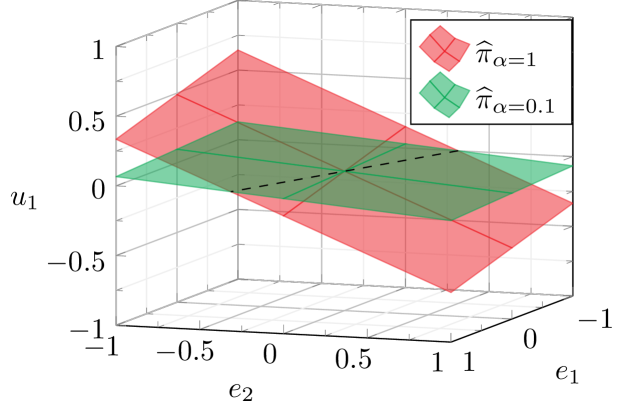
Figure 2: This figure shows the surface of policy $\widehat{\pi}$ in the state space for system (11), which is learned using Alg. 1 with $\alpha=1$ (red surface) and $\alpha=0.1$ (green surface), and the expert being the LQR for system (11).

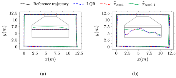
Figure 3: Panel (a) and panel (b) show the trajectory tracking performance for the LQR (dashed blue line), the learned policy $\widehat{\pi}$ learned using Alg. 1 with $\alpha=1$ (dash-dotted red line) and $\alpha=0.1$ (solid green line). In panel (a), the policies are deployed in nominal conditions. The policy $\widehat{\pi}_{\alpha=1}$ performs as good as the LQR while the policy $\widehat{\pi}_{\alpha=0.1}$ performs poorly compared to the LQR and $\widehat{\pi}_{\alpha=1}$. In panel (b), the policies are deployed in non-nominal conditions. The performance of the LQR and policy $\widehat{\pi}_{\alpha=1}$ is worse than when deployed in nominal conditions, while the performance of policy $\widehat{\pi}_{\alpha=0.1}$ in non-nominal conditions remains almost the same as in nominal conditions.

V Numerical experiments

In this section, we present the results from numerical experiments applying our algorithm to (i) learn the Linear Quadratic Regulator (LQR), and (ii) learn nonlinear control for a nonholonomic system (differential drive mobile robot).

V-A Learning the Linear Quadratic Regulator

We consider a vehicle obeying the following dynamics (see also [30] and [38]):

$$\small\begin{split}x_{t+1}\!=\!\underbrace{\begin{bmatrix}1&T_{\text{s}}&0&0\\ 0&1&0&0\\ 0&0&1&T_{\text{s}}\\ 0&0&0&1\end{bmatrix}}_{A}x_{t}\!+\!\underbrace{\begin{bmatrix}0&0\\ T_{\text{s}}&0\\ 0&0\\ 0&T_{\text{s}}\end{bmatrix}}_{B}u_{t},\quad y_{t}=x_{t}+\delta_{t}\end{split}$$ (10)

where $x_{t}\in\mathbb{R}^{4}$ contains the vehicle’s position and velocity in cartesian coordinates, $u_{t}\in\mathbb{R}^{2}$ the input signal, $y\in\mathbb{R}^{4}$ the state measurement, $\delta_{t}\in\mathbb{R}^{4}$ bounded measurement noise with $\|\delta_{t}\|\leq\zeta$ and $\zeta\in\mathbb{R}_{\geq 0}$, and $T_{\text{s}}$ the sampling time. We consider the problem of tracking a reference trajectory, and we write the error dynamics and the controller as

$$e_{t+1}=Ae_{t}+B\bar{u}_{t},\qquad u_{t}=\underbrace{-K(e_{t}+\delta_{t})}_{\bar{u}_{t}}+v_{t},$$ (11)

where $e_{t}=x_{t}-\xi_{t}$ is the error between the system state and the reference state, $\xi_{t}\in\mathbb{R}^{4}$ at time $t$, $v_{t}\in\mathbb{R}^{2}$ is the control input generating $\xi_{t}$, and $K$ denotes the control gain. We consider the expert policy to correspond to the optimal LQR gain, $K_{\text{lqr}}$, which minimizes a discounted value function as in (2) but with horizon $T$, quadratic stage cost $\left.c(e_{t},\bar{u}_{t})=e_{t}^{\mathsf{T}}Qe_{t}+\bar{u}_{t}^{\mathsf{T}}R\bar{u}_{t}\right.$ with error and input weighing matrices $Q\succeq 0$ and $R\succ 0$, respectively. Notice that the quadratic stage cost is strongly convex and Lipschitz bounded over bounded space $e\in B_{r}(0)\subset\mathbb{R}^{4}$ and $\bar{u}\in\mathbb{R}^{2}$.
Expert demonstrations. We generate $N$ expert trajectories using (11) with $K=K_{\text{lqr}}$, $T_{\text{s}}=0.1$, $\gamma=0.82$, $Q=0.1I_{4}$, $R=0.1I_{2}$, and $\delta_{t}=0$, contained in the data matrices $E,U$:

$$E=\left[\begin{matrix}\mathbf{e}^{(1)}&\ldots&\mathbf{e}^{(N)}\end{matrix}\right],\quad U=\left[\begin{matrix}\mathbf{u}^{(1)}&\ldots&\mathbf{u}^{(N)}\end{matrix}\right],$$

with $\mathbf{e}^{(i)}=(e_{0}^{(i)},\ldots,e_{T}^{(i)})$ and $\mathbf{u}^{(i)}=(u_{0}^{(i)},\ldots,u_{T-1}^{(i)})$. Each trajectory is generated with random initial condition, $e_{0}^{(i)}\in B_{2}(0)$ for $i=1,\dots,N$. Note that, since the initial conditions, $e_{0}^{(i)}$, are inside $B_{2}(0)$ and $K=K_{\text{lqr}}$ is stabilizing, then, all the data points in $E$ are inside $B_{2}(0)$.

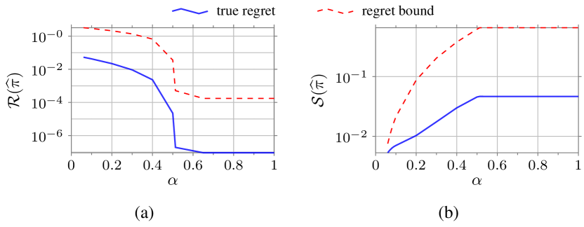
Figure 4: Panel (a) and panel (b) show the true regrets $R(\widehat{\pi})$ and $S(\widehat{\pi})$ in (5) and (6) (solid blue line), and the regret bounds in Theorem III.6 (dashed red line) as a function of the Lipschitz bound, $\alpha$, in (3), respectively. The regret $R(\widehat{\pi})$ and the bound in Theorem III.6-(i) decrease as $\alpha$ increases, as shown in panel (a), while The regret $S(\widehat{\pi})$ the bound in Theorem III.6-(ii) increase with $\alpha$, as shown in panel (b).

Policy learning. Using Alg. 1, we learn policy $\widehat{\pi}$ with $\alpha=1$ and $\alpha=0.1$ denoted by $\widehat{\pi}_{\alpha=1}$ and $\widehat{\pi}_{\alpha=0.1}$, respectively. Fig. 2 shows the surface of the learned policies $\widehat{\pi}_{\alpha=1}$ and $\widehat{\pi}_{\alpha=0.1}$ in the state space. Note that, since the Lipschitz constant of the expert policy, $\pi^{*}=K_{\text{lqr}}$, is $\ell_{\pi^{*}}=\|K_{\text{lqr}}\|_{2}=0.51<\alpha=1$, we get $\|\widehat{\pi}_{\alpha=1}-\pi^{*}\|_{2}=0$, which implies that $\widehat{\pi}_{\alpha=1}$ learns exactly the expert policy. On the other hand, since $\alpha=0.1<\ell_{\pi^{*}}=0.51$, we get $\|\widehat{\pi}_{\alpha=0.1}-\pi^{*}\|_{2}=\epsilon$ for $\epsilon>0$, which implies that $\widehat{\pi}_{\alpha=0.1}$ learns the expert policy with some learning error $\epsilon$. As observed in Fig. 2, the Lipschitz constant constraints the slope of the learned surface, where $\widehat{\pi}_{\alpha=0.1}$ has smaller slope than $\widehat{\pi}_{\alpha=1}$, and hence more robust to perturbations in the states. However, smaller Lipschitz constant implies larger learning error, and hence poorer nominal performance. Fig. 3 shows the trajectory tracking performance for the optimal LQR controller, $\widehat{\pi}_{\alpha=1}$, and $\widehat{\pi}_{\alpha=0.1}$. The policies are deployed in nominal conditions, Fig. 3(a), and in non-nominal conditions with $\zeta=0.5$, Fig. 3(b). We observe in Fig. 3(a) that $\widehat{\pi}_{\alpha=1}$ performs better than $\widehat{\pi}_{\alpha=0.1}$ in nominal conditions. On the other hand, we observe in Fig. 3(b) that the performance of $\widehat{\pi}_{\alpha=1}$ degrades when deployed in non-nominal conditions, while the performance of $\widehat{\pi}_{\alpha=0.1}$ remains almost the same, as predicted by [7].

Regret bounds. The parameters of the bounds in Theorem III.6 are obtained as follows, $\lambda=\max\{\rho(2Q),\rho(2R)\}$, $\alpha^{*}=\|K_{\text{lqr}}\|_{2}$, $\ell_{f}^{u}=\|B\|_{2}$, and $\Theta=\frac{1}{1-\gamma\rho(A+BK)^{2}}$, where $K$ is a stabilizing gain. Fig. 4 shows the regrets ${\mathcal{R}}(\widehat{\pi})$ and ${\mathcal{S}}(\widehat{\pi})$ in (5) and (6), and the corresponding upper bounds derived in Theorem III.6 as a function of the Lipschitz bound, $\alpha$, in (3). As can be seen, the regret ${\mathcal{R}}(\widehat{\pi})$ and the corresponding upper bound in Theorem III.6-(i) decrease as $\alpha$ increases, while the regret ${\mathcal{S}}(\widehat{\pi})$ and the corresponding upper bound in Theorem III.6-(ii) increase with $\alpha$. Further, the regrets and the bounds remains constant for $\alpha\geq 0.51$, since the constraint in (3) becomes inactive and $\widehat{\pi}$ converges to the optimal LQR controller. Fig. 5 shows the tradeoff between the regrets, as well as the tradeoff between the regrets upper bounds as we vary the Lipschitz bound, $\alpha$, in (3). This suggests that improving the robustness of the learned policy to perturbations comes at the expenses of its nominal performance.

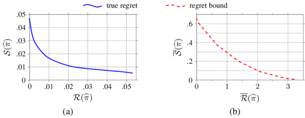
Figure 5: Panel (a) shows the tradeoff between the regrets $R(\widehat{\pi})$ and $S(\widehat{\pi})$ in (5) and (6), respectively. Panel (b) shows the tradeoff between the upper bounds of $R(\widehat{\pi})$ and $S(\widehat{\pi})$ derived in Theorem III.6, respectively.

V-B Learning nonlinear control for nonholonomic system

We consider nonholonomic differential drive mobile robot (see Fig. 6) obeying the following discrete-time nonlinear dynamics

$$\begin{split}x_{t+1}&=T_{s}v_{t}\cos(\theta_{t})+x_{t},\qquad\text{for }t\geq 0\\ y_{t+1}&=T_{s}v_{t}\sin(\theta_{t})+y_{t},\\ \theta_{t+1}&=\theta_{t}+T_{s}\omega_{t}\end{split}$$ (12)

where $x_{t}\in\mathbb{R}$ and $y_{t}\in\mathbb{R}$ are the position of the robot’s centroid in the cartesian coordinate frame $(O;x,y)$, $\theta_{t}\in\mathbb{R}$ is the robot’s orientation, $v_{t}\in\mathbb{R}$ and $\omega_{t}\in\mathbb{R}$ are the robot’s forward and angular velocity at time $t$, respectively, which are the system’s inputs, and $T_{s}>0$ is the sampling time. The dynamics in (12), can be written in the following vector form

$$\begin{split}q_{t+1}=f(q_{t},u_{t}),\qquad u_{t}=\pi(q_{t}+\delta_{t})\qquad\text{for }t\geq 0,\end{split}$$ (13)

where $q_{t}=[x_{t},y_{t},\theta_{t}]^{\mathsf{T}}$ is the state, $u_{t}=[v_{t},\omega_{t}]^{\mathsf{T}}$ is the input, $f:\mathbb{R}^{3}\times\mathbb{R}^{2}\rightarrow\mathbb{R}^{3}$ is the dynamics, $\pi:\mathbb{R}^{3}\rightarrow\mathbb{R}^{2}$ is the control policy, and $\delta_{t}\in\mathbb{R}^{3}$ is a bounded perturbation, with $\|\delta_{t}\|\leq\zeta\in\mathbb{R}_{\geq 0}$. Let $r_{t}=[r^{x}_{t},r^{y}_{t}]^{\mathsf{T}}$ be a point fixed on the robot at a fixed distance $d$ from $[x_{t},y_{t}]^{\mathsf{T}}$ (see Fig. 6). The task is to stabilize the point $r_{t}$ at $[0,0]^{\mathsf{T}}$, which is described by the following regulator problem

$$\begin{split}&\min_{\pi\in\mathrm{Lip}\left(\mathbb{R}^{3};\mathbb{R}^{2}\right)}\;\lim_{T\rightarrow\infty}\sum_{t=0}^{T}\gamma^{t}\left({r_{t}}^{\mathsf{T}}Qr_{t}+{u_{t}}^{\mathsf{T}}\mathcal{R}(\theta_{t})^{\mathsf{T}}R\mathcal{R}(\theta_{t})u_{t}\right),\\ &\qquad\;\text{s.t.}\qquad\begin{cases}q_{t+1}&=f(q_{t},u_{t}),\\ u_{t}&=\pi(q_{t}+\delta_{t}),\end{cases}\end{split}$$ (14)

$$\text{where}\qquad\mathcal{R}(\theta_{t})=\begin{bmatrix}T_{s}\cos(\theta_{t})&-dT_{s}\sin(\theta_{t})\\ T_{s}\sin(\theta_{t})&dT_{s}\cos(\theta_{t})\end{bmatrix}$$

where $\gamma$ is the discount factor, and $Q\succeq 0$ and $R\succ 0$ are weighing matrices.
Expert demonstrations. We consider the expert policy, $\pi^{*}$, to be the minimizer of (LABEL:eq:_nonlinear_control_task). The derivation of $\pi^{*}$ for this example is presented in Appendix A-F.
Policy learning. Using Alg. 1, we learn policy $\widehat{\pi}$ with $\alpha=50$ and $\alpha=0.5$ denoted by $\widehat{\pi}_{\alpha=50}$ and $\widehat{\pi}_{\alpha=0.5}$, respectively. Fig. 7 shows the surface of the learned policies $\widehat{\pi}_{\alpha=50}$ and $\widehat{\pi}_{\alpha=0.5}$ that correspond to the input $\omega$ in the subspace $[x,y]^{\mathsf{T}}$ for $\theta=0$. Since the Lipschitz constant of the expert policy, $\pi^{*}$, is $\ell_{\pi^{*}}=16.65<\alpha=50$, the policy $\widehat{\pi}_{\alpha=50}$ learns exactly the expert policy. On the other hand, since $\alpha=0.5<\ell_{\pi^{*}}=16.65$, the policy $\widehat{\pi}_{\alpha=0.5}$ learns the expert policy with some learning error. As observed in Fig. 7, the Lipschitz constant constraints the slope of the learned surface, where $\widehat{\pi}_{\alpha=0.5}$ has smaller slope than $\widehat{\pi}_{\alpha=50}$, and hence more robust to perturbations in the states. However, since $\widehat{\pi}_{\alpha=0.5}$ has larger learning error, it has poorer nominal performance. Fig. 8 shows the trajectory of the point $(r_{t}^{x},r_{t}^{y})$ (see Fig. 6) induced by the expert policy, $\widehat{\pi}_{\alpha=50}$, and $\widehat{\pi}_{\alpha=0.5}$ starting from initial position $(1,1)$ and an orientation $\theta=180^{\circ}$. The policies are deployed in nominal conditions, Fig. 8(a), and in non-nominal conditions with $\zeta_{r}=0.7$ for the position and $\zeta_{\theta}=\pi/180$ for the orientation, Fig. 8(b). We observe in Fig. 8(a) that $\widehat{\pi}_{\alpha=50}$ performs as good as the expert and better than $\widehat{\pi}_{\alpha=0.5}$ in nominal conditions. On the other hand, we observe in Fig. 8(b) that the performance of $\widehat{\pi}_{\alpha=50}$ and that of the expert degrade when deployed in non-nominal conditions, while the performance of $\widehat{\pi}_{\alpha=0.5}$ remains almost the same.

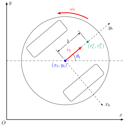
Figure 6: Differential drive mobile robot described in (12).

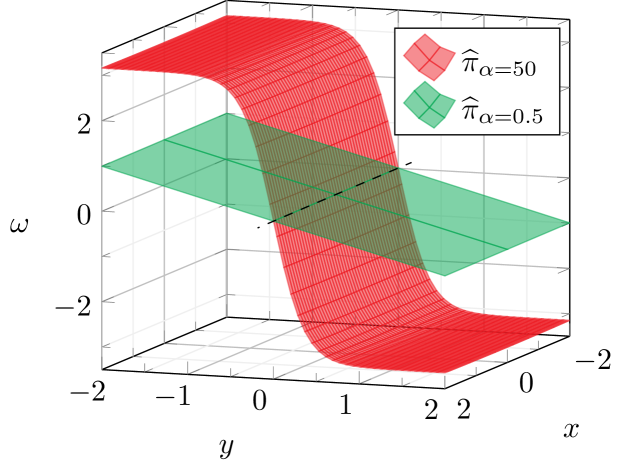
Figure 7: This figure shows the surface of policy $\widehat{\pi}$ that correspond to the input $\omega$ in the subspace $[x,y]^{\mathsf{T}}$ for system (13) for $\theta=0$. Two policies are learned using Alg. 1 with $\alpha=50$ (red surface) and $\alpha=0.5$ (green surface), and the expert demonstrations are generated as in Appendix A-F.

VI Conclusion

In this paper propose a framework to learn feedback control policies with provable robustness guarantees. Our approach draws from our earlier work [7] where we formulate the adversarially robust learning problem as one of Lipschitz-constrained loss minimization. We adapt this framework to the problem of learning robust feedback policies from a dataset obtained from expert demonstrations. We establish robust stability of the closed-loop system under the learned feedback policy. Further, we derive upper bounds on the regret and robustness of the learned feedback policy, which bound its nominal suboptimality with respect to the expert policy and the deterioration of its performance under bounded (adversarial) disturbances to state measurements, respectively. The above bounds suggest the existence of a tradeoff between nominal performance of the feedback policy and closed-loop robustness to adversarial perturbations on the feedback. This tradeoff is also evident in our numerical experiments, where improving closed-loop robustness leads to a deterioration of the nominal performance. Finally, we demonstrate our results and the effectiveness of our robust feedback policy learning framework on several benchmarks.

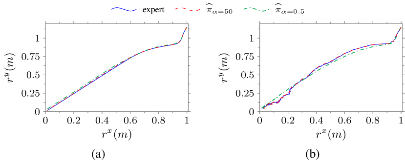
Figure 8: Panel (a) and panel (b) show the trajectory of the expert (solid blue line), the learned policy $\widehat{\pi}$ learned using Alg. 1 with $\alpha=50$ (dashed red line) and $\alpha=0.5$ (dashdotted green line). In panel (a), the policies are deployed in nominal conditions. The policy $\widehat{\pi}_{\alpha=50}$ outputs the same trajectory as the expert while the policy $\widehat{\pi}_{\alpha=0.5}$ outputs a different trajectory towards the equilibrium. In panel (b), the policies are deployed in non-nominal conditions. The performance of the expert and policy $\widehat{\pi}_{\alpha=50}$ is worse than when deployed in nominal conditions, while the performance of policy $\widehat{\pi}_{\alpha=0.5}$ in non-nominal conditions remains almost the same as in nominal conditions.

Appendix

A-A Proof of Lemma III.1

We first note that $V^{*}(x)\geq 0$ for any $x\in\mathbb{R}^{n}$, and $\pi^{*}(0)=0$. To see this, we first recall that $V^{*}(0)\leq\sum_{t=0}^{\infty}\gamma^{t}c(x_{t},u_{t})$ for $x_{t+1}=f(x_{t},u_{t})$ with $x_{0}=0$ and any $\{u_{t}\}$. In particular, with $u_{t}=0$ for all $t\in\mathbb{N}$, we get that $\sum_{t=0}^{\infty}\gamma^{t}c(x_{t},u_{t})=0$ (since $x_{0}=0$, $f(0,0)=0$ and $c(0,0)=0$), and since $0\leq V^{*}(0)\leq\sum_{t=0}^{\infty}\gamma^{t}c(x_{t},u_{t})=0$, it follows that $V^{*}(0)=0$. Now, we have that $\pi^{*}(0)\in\arg\min_{u\in\mathbb{R}^{m}}c(0,u)+V^{*}(f(0,u))$, from which we clearly get that $\pi^{*}(0)=0$ is the only minimizer. Now, since $c$ is $\mu$-strongly convex, with $c(0,0)=0$, we have $c_{\pi^{*}}(x)\geq\mu\|x\|^{2}/2$. Furthermore, since $V^{*}(x)=\min_{u\in\mathbb{R}^{m}}c(x,u)+\gamma V^{*}(f(x,u))$, we get:

$$V^{*}(x) =c_{\pi^{*}}(x)+\gamma V^{*}(f_{\pi^{*}}(x))$$

$$\geq\frac{\mu}{2}\|x\|^{2}+\gamma V^{*}(f_{\pi^{*}}(x))\geq\frac{\mu}{2}\|x\|^{2}.$$

Let $\pi$ be a Lipschitz-continuous (with constant $\alpha$), exponentially stabilizing feedback policy as in Assumption II.1. We then have:

$$V^{*}(x)\leq V_{\pi}(x)=\sum_{t=0}^{\infty}\gamma^{t}c_{\pi}\left(f_{\pi}^{t}(x)\right)\leq\frac{\lambda}{2}\sqrt{1+{\alpha}^{2}}\sum_{t=0}^{\infty}\gamma^{t}\left\|f_{\pi}^{t}(x)\right\|^{2}$$

$$\leq\frac{\lambda}{2}\sqrt{1+{\alpha}^{2}}\sum_{t=0}^{\infty}\left\|f_{\pi}^{t}(x)\right\|^{2}\leq\frac{\lambda}{2}M\sqrt{1+{\alpha}^{2}}\sum_{t=0}^{\infty}\beta^{2t}\|x\|^{2}$$

$$=\frac{\lambda M\sqrt{1+{\alpha}^{2}}}{2(1-\beta^{2})}\|x\|^{2}.$$

We then have:

$$\frac{\mu}{2}\|x\|^{2}\leq V^{*}(x)\leq\frac{\lambda M\sqrt{1+{\alpha}^{2}}}{2(1-\beta^{2})}\|x\|^{2},$$

and the statement of the lemma follows.

A-B Proof of Theorem III.3

(i) Exponential stability under expert (optimal) feedback policy: We now recall that $V^{*}(x)=c_{\pi^{*}}(x)+\gamma V^{*}\left(f_{\pi^{*}}(x)\right)$ and $\underline{\kappa}^{*}\|x\|^{2}\leq V^{*}(x)\leq\bar{\kappa}^{*}\|x\|^{2}$ (from Lemma III.1). It then follows that:

$$V^{*}(f_{\pi^{*}}(x))-V^{*}(x)\leq-\frac{\mu}{2\gamma}\|x\|^{2}+\frac{\bar{\kappa}^{*}(1-\gamma)}{\gamma}\|x\|^{2}$$

$$=-\frac{\bar{\kappa}^{*}}{\gamma}\left[\gamma-\left(1-\frac{\mu}{2\bar{\kappa}^{*}}\right)\right]\|x\|^{2}=-\bar{\kappa}^{*}\left(1-\frac{\gamma^{\prime}}{\gamma}\right)\|x\|^{2}.$$

It follows from the above inequality and the quadratic boundedness of $V^{*}$ that $f_{\pi^{*}}$ is uniformly globally exponentially convergent [39]. In what follows, we obtain an estimate for the upper bound on $\left\|f_{\pi^{*}}^{t}(x)\right\|$. From the above inequality and the fact that $V^{*}(x)\leq\bar{\kappa}^{*}\|x\|^{2}$ we get $V^{*}(f_{\pi^{*}}(x))-V^{*}(x)\leq-(1-\gamma^{\prime}/\gamma)V^{*}(x)$ and $V^{*}(f_{\pi^{*}}(x))\leq\gamma^{\prime}/\gamma V^{*}(x)$. It then follows that $V^{*}(f_{\pi^{*}}^{t}(x))\leq(\gamma^{\prime}/\gamma)^{t}V^{*}(x)$ which implies $\underline{\kappa}^{*}\left\|f_{\pi^{*}}^{t}(x)\right\|^{2}\leq\bar{\kappa}^{*}(\gamma^{\prime}/\gamma)^{t}\|x\|^{2}$. Therefore, we get:

$$\left\|f_{\pi^{*}}^{t}(x)\right\|\leq\sqrt{\frac{\bar{\kappa}^{*}}{\underline{\kappa}^{*}}}\left(\sqrt{\frac{\gamma^{\prime}}{\gamma}}\right)^{t}\|x\|.$$

(ii) Robust stability under learned policy: For $x\in B_{r}(0)$, let $\widehat{x}_{t}=f_{\widehat{\pi}}^{t}(x)$ and $x_{t}^{*}=f_{\pi^{*}}^{t}(x)$. We have:

$$\left\|f_{\widehat{\pi}}(x)\right\|\leq\left\|f_{\pi^{*}}(x)\right\|+\left\|f_{\widehat{\pi}}(x)-f_{\pi^{*}}(x)\right\|$$

$$\leq\sqrt{\frac{\bar{\kappa}^{*}\gamma^{\prime}}{\underline{\kappa}^{*}\gamma}}\|x\|+\ell_{f}^{u}\left\|\widehat{\pi}(x)-\pi^{*}(x)\right\|\leq\sqrt{\frac{\bar{\kappa}^{*}\gamma^{\prime}}{\underline{\kappa}^{*}\gamma}}r+\ell_{f}^{u}\varepsilon.$$

We see that $\left\|f_{\widehat{\pi}}(x)\right\|\leq r$ for $\varepsilon\leq\frac{1}{\ell_{f}^{u}}\left(1-\sqrt{\frac{\bar{\kappa}^{*}\gamma^{\prime}}{\underline{\kappa}^{*}\gamma}}\right)r$. It then follows that $\left\|\widehat{\pi}(\widehat{x}_{t})-\pi^{*}(\widehat{x}_{t})\right\|\leq\varepsilon$ for any $t\in\mathbb{N}$. We then have:

$$\left\|\widehat{x}_{t}\right\| \leq\left(\frac{\bar{\kappa}^{*}\gamma^{\prime}}{\underline{\kappa}^{*}\gamma}\right)^{t/2}\|x\|+\ell_{f}^{u}\sum_{\tau=0}^{t-1}\left(\frac{\bar{\kappa}^{*}\gamma^{\prime}}{\underline{\kappa}^{*}\gamma}\right)^{(t-\tau-1)/2}\varepsilon$$

$$=\left(\sqrt{\frac{\bar{\kappa}^{*}\gamma^{\prime}}{\underline{\kappa}^{*}\gamma}}\right)^{t}\|x\|+\ell_{f}^{u}\left[\frac{1-\left(\sqrt{\frac{\bar{\kappa}^{*}\gamma^{\prime}}{\underline{\kappa}^{*}\gamma}}\right)^{t}}{1-\sqrt{\frac{\bar{\kappa}^{*}\gamma^{\prime}}{\underline{\kappa}^{*}\gamma}}}\right]\varepsilon.$$

Furthermore, we have from part (i) that $x_{t}^{*}\in B_{r}(0)$ for any $t\in\mathbb{N}$. Therefore, $B_{r}(0)$ is invariant under $f_{\pi^{*}}$ and $f_{\widehat{\pi}}$, and we immediately obtain the uniform bound $\left\|\widehat{x}_{t}-x_{t}^{*}\right\|\leq 2r$. We now have:

$$\left\|\widehat{x}_{t}-x_{t}^{*}\right\|=\left\|f(\widehat{x}_{t-1},\widehat{\pi}(\widehat{x}_{t-1}))-f(x_{t-1}^{*},\pi^{*}(x_{t-1}^{*}))\right\|$$

$$\leq\left\|f(\widehat{x}_{t-1},\widehat{\pi}(\widehat{x}_{t-1}))-f(\widehat{x}_{t-1},\pi^{*}(\widehat{x}_{t-1}))\right\|$$

$$\quad+\left\|f(\widehat{x}_{t-1},\pi^{*}(\widehat{x}_{t-1}))-f(x_{t-1}^{*},\pi^{*}(x_{t-1}^{*}))\right\|$$

$$\leq\left\|f_{\pi^{*}}(\widehat{x}_{t-1})-f_{\pi^{*}}(x_{t-1}^{*})\right\|$$

$$\quad+\left\|f(\widehat{x}_{t-1},\widehat{\pi}(\widehat{x}_{t-1}))-f(\widehat{x}_{t-1},\pi^{*}(\widehat{x}_{t-1}))\right\|$$

$$\leq\ell_{f_{\pi^{*}}}\left\|\widehat{x}_{t-1}-x_{t-1}^{*}\right\|+\ell_{f}^{u}\left\|\widehat{\pi}(\widehat{x}_{t-1})-\pi^{*}(\widehat{x}_{t-1})\right\|$$

$$\leq\ell_{f_{\pi^{*}}}\left\|\widehat{x}_{t-1}-x_{t-1}^{*}\right\|+\ell_{f}^{u}\varepsilon$$

$$\leq\ell_{f}^{u}\sum_{\tau=0}^{t-1}\ell_{f_{\pi^{*}}}^{t-\tau-1}\varepsilon=\ell_{f}^{u}\left[\frac{1-\ell_{f_{\pi^{*}}}^{t}}{1-\ell_{f_{\pi^{*}}}}\right]\varepsilon,$$

where the final equality holds for $\ell_{f_{\pi^{*}}}\neq 1$. If $\ell_{f_{\pi^{*}}}=1$, then we have:

$$\left\|\widehat{x}_{t}-x_{t}^{*}\right\|\leq t\cdot\ell_{f}^{u}\varepsilon.$$

We also have:

$$\left\|\widehat{x}_{t}-x_{t}^{*}\right\| \leq\left\|\widehat{x}_{t}\right\|+\left\|x_{t}^{*}\right\|$$

$$\leq 2\left(\sqrt{\frac{\bar{\kappa}^{*}\gamma^{\prime}}{\underline{\kappa}^{*}\gamma}}\right)^{t}\|x\|+\ell_{f}^{u}\left[\frac{1-\left(\sqrt{\frac{\bar{\kappa}^{*}\gamma^{\prime}}{\underline{\kappa}^{*}\gamma}}\right)^{t}}{1-\sqrt{\frac{\bar{\kappa}^{*}\gamma^{\prime}}{\underline{\kappa}^{*}\gamma}}}\right]\varepsilon.$$

Now, for the policy $\widehat{\pi}_{\delta}$, we have $\left\|\widehat{\pi}_{\delta}-\pi^{*}\right\|_{\left(B_{r}(0),\infty\right)}\leq\left\|\widehat{\pi}_{\delta}-\widehat{\pi}\right\|_{\left(B_{r}(0),\infty\right)}+\left\|\widehat{\pi}-\pi^{*}\right\|_{\left(B_{r}(0),\infty\right)}\leq\alpha\zeta+\varepsilon$, and the earlier analysis now carries through with this bound, and the statement of the theorem follows.

A-C Proof of Lemma III.4

From the exponential stability of $f_{\pi}$ and $f_{\pi}$-invariance of $B_{r}(0)$, for $x,x^{\prime}\in B_{r}(0)$, we have $\left\|f_{\pi}^{t}(x)-f_{\pi}^{t}(x^{\prime})\right\|\leq\left\|f_{\pi}^{t}(x)\right\|+\left\|f_{\pi}^{t}(x^{\prime})\right\|\leq 2M\beta^{t}r$. Furthermore, let $\ell_{f_{\pi}}$ be the Lipschitz constant of $f_{\pi}$ on $B_{r}(0)$. This implies that $\left\|f_{\pi}^{t}(x)-f_{\pi}^{t}(x^{\prime})\right\|\leq\ell_{f_{\pi}}^{t}\left\|x-x^{\prime}\right\|$. We then have $\left\|f_{\pi}^{t}(x)-f_{\pi}^{t}(x^{\prime})\right\|\leq\min\left\{\ell_{f_{\pi}}^{t}\left\|x-x^{\prime}\right\|,2M\beta^{t}r\right\}$. We therefore obtain an $M(x_{1},x_{2})$ such that $\left\|f_{\pi}^{t}(x)-f_{\pi}^{t}(x^{\prime})\right\|\leq M(x_{1},x_{2})\beta^{t}\|x_{1}-x_{2}\|$.

A-D Proof of Theorem III.6

The following lemma establishes a difference bound for the value function under a Lipschitz feedback policy:

Lemma A.1 (Value function difference bound).

Let $\pi\in\mathrm{Lip}\left(B_{r}(0);\mathbb{R}^{m}\right)$ be a Lipschitz feedback policy such that $\pi(0)=0$, $\mathrm{lip}(\pi)\leq\alpha$. For the value function $V_{\pi}(x)=\sum_{t=0}^{\infty}\gamma^{t}c_{\pi}\left(f_{\pi}^{t}(x)\right)$ of policy $\pi$, the following holds:

$$\left|V_{\pi}(x^{\prime})-V_{\pi}(x)\right|\leq\Theta\lambda r\sqrt{1+\alpha^{2}}\left\|x^{\prime}-x\right\|\left[1+\frac{\left\|x^{\prime}-x\right\|}{2r}\right],$$

where $\Theta=\sum_{t=0}^{\infty}\gamma^{t}\theta_{t}^{2}$ and $\theta_{t}=M\beta^{t}$.

Proof.

We first note that $(0,0)\in B_{r}(0)\times\mathbb{R}^{m}$ is a strict minimizer of $c$ (by Assumption II.2) and since $c$ is differentiable, we have $\nabla c(0,0)=0$. For any $x\in B_{r}(0)$:

$$\left\|\nabla c_{\pi}(x)\right\|=\left\|\nabla c(x,\pi(x))-\nabla c(0,0)\right\|$$

$$\leq\lambda\left\|(x,\pi(x))\right\|\leq\lambda\sqrt{1+\alpha^{2}}\|x\|,$$

since $\|\pi(x)\|=\|\pi(x)-\pi(0)\|\leq\alpha\|x\|$. For any $x,x^{\prime}\in B_{r}(0)$, let $p$ be the straight line segment between $x$ and $x^{\prime}$, such that $p(t)=x+t(x^{\prime}-x)$ for $t\in[0,1]$. From the $\lambda$-smoothness of $c$, we have:

$$c_{\pi}(x^{\prime}) -c_{\pi}(x)=\int_{0}^{1}\nabla c_{\pi}(p(t))\cdot\dot{p}(t)dt$$

$$\leq\int_{0}^{1}\left\|\nabla c_{\pi}(p(t))\right\|dt\cdot\|x^{\prime}-x\|$$

$$\leq\lambda\sqrt{1+\alpha^{2}}\int_{0}^{1}\|p(t)\|dt\cdot\|x^{\prime}-x\|$$

$$\leq\lambda\sqrt{1+\alpha^{2}}\int_{0}^{1}\|x+t(x^{\prime}-x)\|dt\cdot\|x^{\prime}-x\|$$

$$\leq\lambda\sqrt{1+\alpha^{2}}~{}\|x\|\left\|x^{\prime}-x\right\|+\frac{\lambda}{2}\sqrt{1+\alpha^{2}}\left\|x^{\prime}-x\right\|^{2}$$

We also have:

$$c_{\pi}(x)-c_{\pi}(x^{\prime})\leq \lambda\sqrt{1+\alpha^{2}}~{}\|x^{\prime}\|\left\|x^{\prime}-x\right\|$$

$$+\frac{\lambda}{2}\sqrt{1+\alpha^{2}}\left\|x^{\prime}-x\right\|^{2},$$

and therefore we get:

$$\left|c_{\pi}(x)-c_{\pi}(x^{\prime})\right|\leq \lambda\sqrt{1+\alpha^{2}}~{}\max\{\|x\|,\|x^{\prime}\|\}\left\|x^{\prime}-x\right\|$$

$$+\frac{\lambda}{2}\sqrt{1+\alpha^{2}}\left\|x^{\prime}-x\right\|^{2}.$$

We now have:

$$\footnotesize\begin{aligned} &V_{\pi}(x^{\prime})-V_{\pi}(x)=\sum_{t=0}^{\infty}\gamma^{t}\left[c_{\pi}\left(f_{\pi}^{t}(x^{\prime})\right)-c_{\pi}\left(f_{\pi}^{t}(x)\right)\right]\\ &\leq\sum_{t=0}^{\infty}\gamma^{t}\bigg{[}\lambda\sqrt{1+\alpha^{2}}~{}\max\{\|f_{\pi}^{t}(x)\|,\|f_{\pi}^{t}(x^{\prime})\|\}\left\|f_{\pi}^{t}(x^{\prime})-f_{\pi}^{t}(x)\right\|\\ &\qquad\qquad~{}+\frac{\lambda}{2}\sqrt{1+\alpha^{2}}\left\|f_{\pi}^{t}(x^{\prime})-f_{\pi}^{t}(x)\right\|^{2}\bigg{]}\\ &\leq\left[\sum_{t=0}^{\infty}\gamma^{t}\theta_{t}^{2}\right]\lambda\sqrt{1+\alpha^{2}}~{}\max\{\|x\|,\|x^{\prime}\|\}\left\|x^{\prime}-x\right\|\\ &\quad+\left[\sum_{t=0}^{\infty}\gamma^{t}\theta_{t}^{2}\right]\frac{\lambda}{2}\sqrt{1+\alpha^{2}}\left\|x^{\prime}-x\right\|^{2}\\ &\leq\Theta\lambda\sqrt{1+\alpha^{2}}~{}r\left\|x^{\prime}-x\right\|+\frac{1}{2}\Theta\lambda\sqrt{1+\alpha^{2}}\left\|x^{\prime}-x\right\|^{2},\end{aligned}$$

and the statement of the lemma follows. ∎

(i) Regret: Let $\pi\in\mathrm{Lip}\left(B_{r}(0),\mathbb{R}^{m}\right)$ be a policy such that $\left\|\pi-\pi^{*}\right\|\leq\varepsilon$ and $\mathrm{lip}(\pi)\leq\alpha$. Since $\varepsilon\leq\frac{1}{\ell_{f}^{u}}\left(1-\sqrt{\frac{\bar{\kappa}^{*}\bar{\gamma}}{\underline{\kappa}^{*}\gamma}}\right)r$, we get from Theorem III.3 that $B_{r}(0)$ is $f_{\pi}$-invariant. The value function $V_{\pi}$ corresponding to $\pi$ satisfies $V_{\pi}(x)=c_{\pi}\big{(}x\big{)}+\gamma V_{\pi}\big{(}f_{\pi}(x)\big{)}$. We then have for any $x\in B_{r}(0)$:

$$\mathcal{R}(\pi)=\sup_{x\in B_{r}(0)}\left\{V_{\pi}(x)-V^{*}(x)\right\}$$

$$=\sup_{x\in B_{r}(0)}\left\{c_{\pi}(x)-c_{\pi^{*}}(x)+\gamma\left(V_{\pi}(f_{\pi}(x))-V^{*}(f_{\pi^{*}}(x))\right)\right\}$$

$$\leq\sup_{x\in B_{r}(0)}\left\{c_{\pi}(x)-c_{\pi^{*}}(x)+\gamma\left(V_{\pi}(f_{\pi}(x))-V^{*}(f_{\pi}(x))\right)\right.$$

$$\qquad\qquad\left.+\gamma\left(V^{*}(f_{\pi}(x))-V^{*}(f_{\pi^{*}}(x))\right)\right\}$$

$$\leq\sup_{x\in B_{r}(0)}\left\{c_{\pi}(x)-c_{\pi^{*}}(x)+\gamma\left(V^{*}(f_{\pi}(x))-V^{*}(f_{\pi^{*}}(x))\right)\right.$$

$$\qquad\qquad+\gamma\sup_{x\in B_{r}(0)}\left\{V_{\pi}(x)-V^{*}(x)\right\}\}.$$

It then follows that:

$$\mathcal{R}(\pi)\leq\frac{1}{1-\gamma}\cdot\sup_{x\in B_{r}(0)}\{c_{\pi}(x)-c_{\pi^{*}}(x)$$

$$\qquad\qquad\qquad\qquad\qquad\;+\gamma\left(V^{*}(f_{\pi}(x))-V^{*}(f_{\pi^{*}}(x))\right)\}.$$

Furthermore, we have:

$$\sup_{x\in B_{r}(0)}\{c_{\pi}(x)-c_{\pi^{*}}(x)\}$$

$$~{}\leq\lambda\sqrt{1+\left|\max\left\{\alpha,\alpha^{*}\right\}\right|^{2}}~{}r\left\|\pi-\pi^{*}\right\|_{\infty}+\frac{\lambda}{2}\left\|\pi-\pi^{*}\right\|_{\infty}^{2}.$$

From Lemma A.1, we also have:

$$\small\begin{aligned} &V^{*}(f_{\pi}(x))-V^{*}(f_{\pi^{*}}(x))\\ &\qquad\quad\leq\Theta\lambda r\sqrt{1+{\alpha^{*}}^{2}}\left\|f_{\pi}(x)-f_{\pi^{*}}(x)\right\|\left[1+\frac{\left\|f_{\pi}(x)-f_{\pi^{*}}(x)\right\|}{2r}\right]\\ &\qquad\quad\leq\Theta\lambda r\sqrt{1+{\alpha^{*}}^{2}}~{}\ell_{f}^{u}\left\|\pi-\pi^{*}\right\|_{\infty}\left[1+\frac{\ell_{f}^{u}\left\|\pi-\pi^{*}\right\|_{\infty}}{2r}\right].\end{aligned}$$

The statement of the theorem follows from the above two inequalities.

(ii) Robustness: The value function for the policy $\pi$ satisfies $V_{\pi}(x)=c_{\pi}\big{(}x\big{)}+\gamma V_{\pi}\big{(}f_{\pi}(x)\big{)}$. For convenience of notation, we denote $\pi\circ(\operatorname{Id}+\delta)$ by $\pi_{\delta}$, i.e., $\pi_{\delta}(x)=\pi(x+\delta)$. For $\|\delta\|_{\infty}\leq\zeta\in\mathbb{R}$, we have:

$$\mathcal{S}(\pi)=\sup_{x\in B_{r}(0)}\left\{V_{\pi_{\delta}}\big{(}x\big{)}-V_{\pi}\big{(}x\big{)}\right\}$$

$$=\sup_{x\in B_{r}(0)}\left\{c_{\pi_{\delta}}(x)-c_{\pi}(x)+\gamma\left(V_{\pi_{\delta}}\big{(}f_{\pi_{\delta}}(x)\big{)}-V_{\pi}\big{(}f_{\pi}(x)\big{)}\right)\right\}$$

$$\leq\sup_{x\in B_{r}(0)}\left\{c_{\pi_{\delta}}(x)-c_{\pi}(x)+\gamma\left(V_{\pi_{\delta}}\left(f_{\pi_{\delta}}(x)\right)-V_{\pi}\left(f_{\pi_{\delta}}(x)\right)\right)\right.$$

$$\qquad\qquad\left.+\gamma\left(V_{\pi}\left(f_{\pi_{\delta}}(x)\right)-V_{\pi}\left(f_{\pi}(x)\right)\right)\right\}$$

$$\leq\left.\sup_{x\in B_{r}(0)}\right\{c_{\pi_{\delta}}(x)-c_{\pi}(x)+\gamma\left(V_{\pi}\left(f_{\pi_{\delta}}(x)\right)-V_{\pi}\left(f_{\pi}(x)\right)\right)$$

$$\qquad\qquad\left.+\gamma\sup_{x\in B_{r}(0)}\left\{V_{\pi_{\delta}}\left(f_{\pi_{\delta}}(x)\right)-V_{\pi}\left(f_{\pi_{\delta}}(x)\right)\right\}\right\}.$$

It then follows that:

$$\mathcal{S}(\pi)=\frac{1}{1-\gamma}\cdot\sup_{x\in B_{r}(0)}\{c_{\pi_{\delta}}(x)-c_{\pi}(x)$$

$$\qquad\qquad\qquad\qquad\qquad+\gamma\left(V_{\pi}\left(f_{\pi_{\delta}}(x)\right)-V_{\pi}\left(f_{\pi}(x)\right)\right)\}.$$

Furthermore, we have:

$$\sup_{x\in B_{r}(0)}\{c_{\pi_{\delta}}(x)-c_{\pi}(x)\}\leq\lambda\alpha\sqrt{1+\alpha^{2}}~{}r\zeta+\frac{\lambda}{2}\alpha^{2}\zeta^{2}.$$

From Lemma A.1, we also have:

$$\small\begin{aligned} &V_{\pi}\left(f_{\pi_{\delta}}(x)\right)-V_{\pi}\left(f_{\pi}(x)\right)\\ &\qquad\quad\leq\Theta\lambda r\sqrt{1+\alpha^{2}}\left\|f_{\pi_{\delta}}(x)-f_{\pi}(x)\right\|\left[1+\frac{\left\|f_{\pi_{\delta}}(x)-f_{\pi}(x)\right\|}{2r}\right]\\ &\qquad\quad\leq\Theta\lambda r\sqrt{1+\alpha^{2}}~{}\ell_{f}^{u}\alpha\zeta\left[1+\frac{\ell_{f}^{u}\alpha\zeta}{2r}\right].\end{aligned}$$

The statement of the theorem follows from the above two inequalities.

A-E Proof of Theorem IV.1

We first let $X_{N}=\{\mathbf{x}^{(1)},\ldots,\mathbf{x}^{(N)}\}$ where $\mathbf{x}^{(i)}=\left(x^{(i)}_{0},\ldots,x^{(i)}_{T-1}\right)$ and $\rho(X_{N},r)$ the covering radius for the set $X_{N}$ w.r.t. the ball $B_{r}(0)$, defined as follows:

$$\rho(X_{N},r)=\sup_{x\in B_{r}(0)}~{}\min_{\begin{subarray}{c}i\in\{1,\ldots,N\},\\ t\in\{0,\ldots,T-1\}\end{subarray}}\left|x-x^{(i)}_{t}\right|.$$

(a) From Lipschitz bound to covering radius: For any $i\in\{1,\ldots,N\}$ and $t\in\{0,\ldots,T-1\}$, we have:

$$|\widehat{\pi}(x)-\pi^{*}(x)|$$

$$=\left|\widehat{\pi}(x)-\widehat{\pi}(x^{(i)}_{t})+\widehat{\pi}(x^{(i)}_{t})-\pi^{*}(x^{(i)}_{t})+\pi^{*}(x^{(i)}_{t})-\pi^{*}(x)\right|$$

$$\leq(\alpha+\alpha^{*})\left|x-x^{(i)}_{t}\right|+\left|\widehat{\pi}(x^{(i)}_{t})-\pi^{*}(x^{(i)}_{t})\right|.$$

In particular, the following holds:

$$|\widehat{\pi}(x)-\pi^{*}(x)|$$

$$\leq\min_{\begin{subarray}{c}i\in\{1,\ldots,N\},\\ t\in\{0,\ldots,T-1\}\end{subarray}}\left[(\alpha+\alpha^{*})\left|x-x_{i}\right|+\left|\widehat{\pi}(x_{i})-\pi^{*}(x_{i})\right|\right]$$

$$\leq(\alpha+\alpha^{*})\min_{\begin{subarray}{c}i\in\{1,\ldots,N\},\\ t\in\{0,\ldots,T-1\}\end{subarray}}\left|x-x_{i}\right|+\max_{\begin{subarray}{c}i\in\{1,\ldots,N\},\\ t\in\{0,\ldots,T-1\}\end{subarray}}\left|\widehat{\pi}(x_{i})-\pi^{*}(x_{i})\right|$$

$$\leq(\alpha+\alpha^{*})\min_{\begin{subarray}{c}i\in\{1,\ldots,N\},\\ t\in\{0,\ldots,T-1\}\end{subarray}}\left|x-x_{i}\right|+\varepsilon_{\rm train}.$$

where

$$\varepsilon_{\rm train}(\widehat{\pi})=\max_{\begin{subarray}{c}i\in\{1,\ldots,N\},\\ t\in\{0,\ldots,T-1\}\end{subarray}}\left\|\widehat{\pi}(x_{t}^{(i)})-\pi^{*}(x_{t}^{(i)})\right\|.$$

Therefore, we get:

$$\sup_{x\in B_{r}(0)} \left|\widehat{\pi}(x)-\pi^{*}(x)\right|$$

$$\leq(\alpha+\alpha^{*})\sup_{x\in B_{r}(0)}~{}\min_{\begin{subarray}{c}i\in\{1,\ldots,N\},\\ t\in\{0,\ldots,T-1\}\end{subarray}}\left|x-x^{(i)}_{t}\right|+\varepsilon_{\rm train}.$$

From the previous inequality, we obtain the following probabilistic bound:

$$\mathbb{P}\Bigg{[}\sup_{x\in B_{r}(0)}\left|\widehat{\pi}(x)-\pi^{*}(x)\right|>(\alpha+\alpha^{*})\delta+\varepsilon_{\rm train}\Bigg{]}\leq\mathbb{P}\left[\rho(X_{N},r)>\delta\right].$$

In what follows, we obtain an upper bound for the quantity on the right hand side of the inequality above.

(b) Probability bound for disjoint intersections: Let $Q_{1},\ldots,Q_{m}$ be disjoint subsets of $B_{r}(0)$ and let $E_{k}$ be the event $Q_{k}\cap X_{N}=\emptyset$. We then have:

$$\mathbb{P}\left[\cup_{k=1}^{m}E_{k}\right]=\sum_{k=1}^{m}(-1)^{k+1}\sum_{\left(j_{1},\ldots,j_{k}\right)}\mathbb{P}\left[E_{j_{1}}\cap\ldots\cap E_{j_{k}}\right].$$

For any $k$-tuple $\left(j_{1},\ldots,j_{k}\right)$, the event $E_{j_{1}}\cap\ldots\cap E_{j_{k}}$ occurs if the points $x_{1},\ldots,x_{N}$ are in the complement of $E_{j_{1}}\cup\ldots\cup E_{j_{k}}$. We then have:

$$\mathbb{P}\left[E_{j_{1}}\cap\ldots\cap E_{j_{k}}\right]=\left[1-\sum_{i=1}^{k}\frac{\mathrm{Vol}\left(Q_{j_{i}}\right)}{\mathrm{Vol}\left(B_{r}(0)\right)}\right]^{N}.$$

For any $k\in\{1,\ldots,m\}$, let $c\leq\mathrm{Vol}\left(Q_{k}\right)\leq C$. We then have:

$${m\choose k}\bigg{[}1-\frac{k\cdot C}{\mathrm{Vol}\left(B_{r}(0)\right)}\bigg{]}^{N}$$

$$\leq\sum_{\left(j_{1},\ldots,j_{k}\right)}\mathbb{P}\left[E_{j_{1}}\cap\ldots\cap E_{j_{k}}\right]\leq{m\choose k}\left[1-\frac{k\cdot c}{\mathrm{Vol}\left(B_{r}(0)\right)}\right]^{N}.$$

It follows from the above that:

$$\mathbb{P}\left[\cup_{k=1}^{m}E_{k}\right]\leq\sum_{k=1}^{m}(-1)^{k+1}{m\choose k}\left[1-\frac{k\cdot c(k)}{\mathrm{Vol}\left(B_{r}(0)\right)}\right]^{N},$$ (15)

where $c(k)=c$ when $k$ is odd and $c(k)=C$ when $k$ is even.

(c) Probabilistic bound for covering radius: We now use the bound (15) derived in (ii) to obtain a probabilistic bound for the covering radius of $X_{N}$ w.r.t. $B_{r}(0)$. Let $\mathcal{E}_{\delta}\subset B_{r}(0)$ be a maximal set of points in $B_{r}(0)$ such that for any $z_{1},z_{2}\in\mathcal{E}_{\delta}$, we have $d(z_{1},z_{2})\geq\delta$. Then, for any $x\in B_{r}(0)\setminus\mathcal{E}_{\delta}$, there exists $z\in\mathcal{E}_{\delta}$ such that $d(x,z)<\delta$ (since $\mathcal{E}_{\delta}$ is maximal, i.e., if $d(x,z)\geq\delta$ we will have $x\in\mathcal{E}_{\delta}$ and we will obtain a contradiction). We note that $\mathcal{E}_{\delta}$ is a discrete set with $\left|\mathcal{E}_{\delta}\right|$ points (where $\left|\mathcal{E}_{\delta}\right|$ is the cardinality of $\mathcal{E}_{\delta}$). We note that:

$$\mathrm{Vol}\left(B_{r}(0)\right) \geq\sum_{z_{k}\in\mathcal{E}_{\delta}}\mathrm{Vol}\left(B_{r}(0)\cap B_{\delta/2}(z_{k})\right)$$

$$\geq\left|\mathcal{E}_{\delta}\right|\cdot\mathrm{Vol}\left(B_{r}(0)\cap B_{\delta/2}(z\in\partial B_{r}(0))\right).$$

We therefore get:

$$\left|\mathcal{E}_{\delta}\right|\leq\frac{\mathrm{Vol}\left(B_{r}(0)\right)}{\mathrm{Vol}\left(B_{r}(0)\cap B_{\delta/2}(z\in\partial B_{r}(0))\right)}.$$

Furthermore, if $\rho(X_{N},r)>\delta$, there exists an $x\in B_{r}(0)$ such that $B_{\delta}(x)\cap X_{N}=\emptyset$. Now we can choose $z\in\mathcal{E}_{\delta/2}$ such that $d(x,z)<\delta/2$ and it follows that $B_{\delta/2}(z)\cap X_{N}=\emptyset$. Let $E_{k}$ be the event $X_{N}\cap B_{\delta/2}(z_{k})=\emptyset$, where $\mathcal{E}_{\delta/2}=\{z_{1},\ldots,z_{\left|\mathcal{E}_{\delta/2}\right|}\}$.

Now, we note that the dataset $X_{N}$ consists of $N$ closed-loop trajectories of length $T$, generated by the optimal policy $\pi^{*}$. Now for any $Q\subseteq B_{r}(0)$ and any $t\in\{0,\ldots,T-1\}$, we have $x_{t}\in Q$ if and only if $x_{0}\in\left(f_{\pi^{*}}^{t}\right)^{-1}Q$. It then follows that a closed-loop trajectory $(x_{0},\ldots,x_{T-1})$, generated by the optimal policy $\pi^{*}$, intersects with $Q$ if and only if $x_{0}\in B_{r}(0)\cap\left(\cup_{t=0}^{T-1}\left(f_{\pi^{*}}^{t}\right)^{-1}Q\right)$. We now obtain bounds on:

$$\mathrm{Vol}\left(B_{r}(0)\cap\left(\cup_{t=0}^{T-1}\left(f_{\pi^{*}}^{t}\right)^{-1}Q\right)\right).$$

Owing to contractivity of the closed-loop dynamics $f_{\pi^{*}}$, it attains a maximum for $Q=B_{\delta/2}(0)$. We have:

$$\bar{\kappa}^{*}\left\|f_{\pi^{*}}(x)\right\|^{2} \geq V^{*}\left(f_{\pi^{*}}(x)\right)=-\frac{1}{\gamma}c_{\pi^{*}}(x)+\frac{1}{\gamma}V^{*}(x)$$

$$\geq\frac{\underline{\kappa}^{*}-\lambda\sqrt{1+{\alpha^{*}}^{2}}/2}{\gamma}\|x\|^{2}.$$

It then follows that:

$$\left\|f_{\pi^{*}}^{t}(x)\right\|\geq\left[\underbrace{\sqrt{\frac{\underline{\kappa}^{*}-\lambda\sqrt{1+{\alpha^{*}}^{2}}/2}{\gamma\bar{\kappa}^{*}}}}_{\nu}\right]^{t}\|x\|,$$

Then, the supremum of the volume is given by $C=\mathrm{Vol}\left(B_{r}(0)\cap B_{\delta/2\nu^{T}}(0)\right)$. Also, it attains a minimum for $Q=B_{\delta}(z\in\partial B_{r}(0))$, which is lower bounded by $c=\mathrm{Vol}\left(B_{r}(0)\cap B_{\delta/2}(z\in\partial B_{r}(0))\right)$. We then have:

$$\mathbb{P}[\rho( X_{N},r)>\delta]=\mathbb{P}\left[\exists~{}x\in B_{r}(0)\;:\;B_{\delta}(x)\cap X_{N}=\emptyset\right]$$

$$\leq\mathbb{P}\left[\cup_{k=1}^{\left|\mathcal{E}_{\delta/2}\right|}E_{k}\right]$$

$$\leq\sum_{k=1}^{\left|\mathcal{E}_{\delta/2}\right|}(-1)^{k+1}{\left|\mathcal{E}_{\delta/2}\right|\choose k}\left[1-\frac{k\cdot c(k)}{\mathrm{Vol}\left(B_{r}(0)\right)}\right]^{N},$$

and the statement of the theorem follows.

A-F Expert policy for the system in subsection V-B

In this subsection, we present more details for the numerical example in subsection V-B. The expert’s task is to stabilize the point $r_{t}=[r^{x}_{t},r^{y}_{t}]^{\mathsf{T}}$ at $[0,0]^{\mathsf{T}}$ with minimal cost (LABEL:eq:_nonlinear_control_task). Knowing that $r^{x}_{t}=x_{t}+d\cos(\theta_{t})$ and $r^{y}_{t}=y_{t}+d\sin(\theta_{t})$ and using (12), we can describe the dynamics of $r^{x}_{t}$ and $r^{y}_{t}$ as

$$\underbrace{\begin{bmatrix}r^{x}_{t+1}\\ r^{y}_{t+1}\end{bmatrix}}_{r_{t+1}}=\underbrace{\begin{bmatrix}r^{x}_{t}\\ r^{y}_{t}\end{bmatrix}}_{r_{t}}+\underbrace{\begin{bmatrix}T_{s}\cos(\theta_{t})&-dT_{s}\sin(\theta_{t})\\ T_{s}\sin(\theta_{t})&dT_{s}\cos(\theta_{t})\end{bmatrix}}_{\mathcal{R}(\theta_{t})}\underbrace{\begin{bmatrix}v_{t}\\ \omega_{t}\end{bmatrix}}_{u_{t}},$$ (16)

Where we assumed that $T_{s}$ is very small and used the approximation $\sin(T_{s}\omega_{t})\approx T_{s}\omega_{t}$ and $\cos(T_{s}\omega_{t})\approx 1$. Let $[v_{t},\omega_{t}]^{\mathsf{T}}=\mathcal{R}^{-1}[\mu^{x}_{t},\mu^{x}_{t}]^{\mathsf{T}}$, then (16) is written as

$$r_{t+1}=r_{t}+\mu_{t},\quad\text{where}\quad\mu_{t}=[\mu^{x}_{t},\mu^{y}_{t}]^{\mathsf{T}}.$$ (17)

To stabilize $r_{t}$ at $[0,0]^{\mathsf{T}}$, we design $\mu_{t}=-Kr_{t}$, where $K$ is a gain matrix that minimizes (LABEL:eq:_nonlinear_control_task), which can be rewritten as

$$\begin{split}&\min_{\mu\in\mathrm{Lip}\left(\mathbb{R}^{2};\mathbb{R}^{2}\right)}\qquad\lim_{T\rightarrow\infty}\sum_{t=0}^{T}\gamma^{t}\left({r_{t}}^{\mathsf{T}}Qr_{t}+{\mu_{t}}^{\mathsf{T}}R\mu_{t}\right),\\ &\qquad\text{s.t.}\qquad\qquad r_{t+1}=r_{t}+\mu_{t},\end{split}$$ (18)

We generate $N$ expert trajectories using (13) with $u_{t}=-\mathcal{R}^{-1}(\theta_{t})Kr_{t}$, where $K$ is the LQR gain matrix that minimizes (18) with $T_{s}=0.01$, $d=0.15$, $\gamma=0.8$, $Q=I_{2}$, $R=300I_{2}$, and $\delta=0$. The generated trajectories are contained in the matrices

$$E=\left[\begin{matrix}\mathbf{q}^{(1)}&\ldots&\mathbf{q}^{(N)}\end{matrix}\right],\quad U=\left[\begin{matrix}\mathbf{u}^{(1)}&\ldots&\mathbf{u}^{(N)}\end{matrix}\right],$$

with $\mathbf{q}^{(i)}=(q_{0}^{(i)},\ldots,q_{T}^{(i)})$ and $\mathbf{u}^{(i)}=(u_{0}^{(i)},\ldots,u_{T-1}^{(i)})$. Each trajectory is generated with random initial condition, $[x_{0}^{(i)},y_{0}^{(i)}]^{\mathsf{T}}\in B_{2}(0)$ and $\theta_{0}^{(i)}\in B_{\pi}(0)$ for $i=1,\dots,N$.

References

- [1] M. Fazlyab, A. Robey, H. Hassani, M. Morari, and G. J. Pappas. Efficient and accurate estimation of Lipschitz constants for deep neural networks. In Advances in Neural Information Processing Systems, pages 11423–11434, 2019.
- [2] S. Aziznejad, H. Gupta, J. Campos, and M. Unser. Deep neural networks with trainable activations and controlled lipschitz constant. IEEE Transactions on Signal Processing, 68:4688–4699, 2020.
- [3] P. L. Combettes and J-C. Pesquet. Lipschitz certificates for layered network structures driven by averaged activation operators. SIAM Journal on Mathematics of Data Science, 2(2):529–557, 2020.
- [4] L. Bungert, R. Raab, T. Roith, L. Schwinn, and D. Tenbrinck. Clip: Cheap lipschitz training of neural networks. In International Conference on Scale Space and Variational Methods in Computer Vision, pages 307–319, 2021.
- [5] Y. Yoshida and T. Miyato. Spectral norm regularization for improving the generalizability of deep learning. arXiv preprint arXiv:1705.10941, 2017.
- [6] H. Gouk, E. Frank, B. Pfahringer, and M. J. Cree. Regularisation of neural networks by enforcing lipschitz continuity. Machine Learning, 110(2):393–416, 2021.
- [7] V. Krishnan, A. A. Al Makdah, and F. Pasqualetti. Lipschitz bounds and provably robust training by laplacian smoothing. In Advances in Neural Information Processing Systems, volume 33, pages 10924–10935, Vancouver, Canada, December 2020.
- [8] C. Szegedy, W. Zaremba, I. Sutskever, J. Bruna, D. Erhan, I. Goodfellow, and R. Fergus. Intriguing properties of neural networks. In International Conference on Learning Representations, Banff, Canada, Apr 2014.
- [9] T. W. Weng, H. Zhang, P. Y. Chen, J. Yi, D. Su, Y. Gao, C. J. Hsieh, and L. Daniel. Evaluating the robustness of neural networks: An extreme value theory approach. In International Conference on Learning Representations, Vancouver Convention Center, BC, Canada, May 2018.
- [10] F. Berkenkamp, M. Turchetta, A. Schoellig, and A. Krause. Safe model-based reinforcement learning with stability guarantees. In Advances in Neural Information Processing Systems, pages 908–918, 2017.
- [11] M. Jin and J. Lavaei. Stability-certified reinforcement learning: A control-theoretic perspective. IEEE Access, 8:229086–229100, 2020.
- [12] D. A. Pomerleau. Alvinn: An autonomous land vehicle in a neural network. In D. Touretzky, editor, Advances in Neural Information Processing Systems, volume 1, Denver, CO, USA, Nov. 1989. Morgan-Kaufmann.
- [13] S. Ross and D. Bagnell. Efficient reductions for imitation learning. In Proceedings of the thirteenth international conference on artificial intelligence and statistics, pages 661–668. JMLR Workshop and Conference Proceedings, 2010.
- [14] S. Ross, G. Gordon, and D. Bagnell. A reduction of imitation learning and structured prediction to no-regret online learning. In Proceedings of the conference on artificial intelligence and statistics, pages 627–635. JMLR Workshop and Conference Proceedings, 2011.
- [15] S. Schaal. Is imitation learning the route to humanoid robots? Trends in Cognitive Sciences, 3(6):233–242, 1999.
- [16] F. Codevilla, M. Müller, A. López, V. Koltun, and A. Dosovitskiy. End-to-end driving via conditional imitation learning. In International Conference on Robotics and Automation (ICRA), pages 4693–4700. IEEE, 2018.
- [17] P. Abbeel and A. Y. Ng. Apprenticeship learning via inverse reinforcement learning. In Proceedings of International Conference on Machine Learning, Banff, AB, Canada, Jul. 2004.
- [18] P. Abbeel, D. Dolgov, A. Y. Ng, and S. Thrun. Apprenticeship learning for motion planning with application to parking lot navigation. In IEEE/RSJ International Conference on Intelligent Robots and Systems, pages 1083–1090, Nice, France, Sep. 2008.
- [19] U. Syed and R. E. Schapire. A game-theoretic approach to apprenticeship learning. In J. Platt, D. Koller, Y. Singer, and S. Roweis, editors, Advances in Neural Information Processing Systems, volume 20, Vancouver, BC, Canada, Dec. 2008. Curran Associates, Inc.
- [20] S. Levine, Z. Popovic, and V. Koltun. Nonlinear inverse reinforcement learning with gaussian processes. In J. S. Taylor, R. Zemel, P. Bartlett, F. Pereira, and K. Q. Weinberger, editors, Advances in Neural Information Processing Systems, volume 24, Granda, Spain, Dec. 2011. Curran Associates, Inc.
- [21] J. Ho, J. Gupta, and S. Ermon. Model-free imitation learning with policy optimization. In M. F. Balcan and K. Q. Weinberger, editors, Proceedings of International Conference on Machine Learning, volume 48 of Proceedings of Machine Learning Research, pages 2760–2769, New York, NY, USA, Jun. 2016. PMLR.
- [22] B. D. Ziebart, A. Maas, J. A. Bagnell, and A. K. Dey. Maximum entropy inverse reinforcement learning. In Proceedings of AAAI Conference on Artificial Intelligence, pages 1433–1438, Chicago, IL, USA, Jul. 2008. AAAI.
- [23] S. Ross, G. J. Gordon, and J. A. Bagnell. A reduction of imitation learning and structured prediction to no-regret online learning. In Proceedings of International Conference on Artificial Intelligence and Statistics, volume 15 of Proceedings of Machine Learning Research, pages 627–635, Fort Lauderdale, FL, USA, Apr. 2011. PMLR.
- [24] M. Laskey, J. Lee, R. Fox, A. Dragan, and K. Goldberg. Dart: Noise injection for robust imitation learning. arXiv preprint arXiv:1703.09327, 2017.
- [25] P. Tigas, A. Filos, R. McAllister, N. Rhinehart, S. Levine, and Y. Gal. Robust imitative planning: Planning from demonstrations under uncertainty. arXiv preprint arXiv:1907.01475, 2019.
- [26] I. Kostrikov, K. K. Agrawal, D. Dwibedi, S. Levine, and J. Tompson. Discriminator-actor-critic: Addressing sample inefficiency and reward bias in adversarial imitation learning. arXiv preprint arXiv:1809.02925, 2018.
- [27] K. Zolna, S. Reed, A. Novikov, S. G. Colmenarej, D. Budden, S. Cabi, M. Denil, N. de Freitas, and Z. Wang. Task-relevant adversarial imitation learning. arXiv preprint arXiv:1910.01077, 2019.
- [28] J. Wang, Z. Zhuang, Y. Wang, and H. Zhao. Adversarially robust imitation learning. In Conference on Robot Learning, London,UK, Nov. 2021.
- [29] L. Lindemann, A. Robey, L. Jiang S. Tu, and N. Matni. Learning robust output control barrier functions from safe expert demonstrations. arXiv preprint arXiv:2102.09971, 2021.
- [30] A. A. Al Makdah, V. Katewa, and F. Pasqualetti. Accuracy prevents robustness in perception-based control. In American Control Conference, Denver, CO, USA, July 2020.
- [31] L. Hewing, K. Wabersich, M. Menner, and M. Zeilinger. Learning-based model predictive control: Toward safe learning in control. Annual Review of Control, Robotics, and Autonomous Systems, 3:269–296, 2020.
- [32] S. Tu, A. Robey, T. Zhang, and N. Matni. On the sample complexity of stability constrained imitation learning. arXiv preprint arXiv:2102.09161v2, 2021.
- [33] S. Dean, N. Matni, B. Recht, and V. Ye. Robust guarantees for perception-based control. arXiv preprint arXiv:1907.03680, 2019.
- [34] F. Pasqualetti, F. Dörfler, and F. Bullo. Attack detection and identification in cyber-physical systems. IEEE Transactions on Automatic Control, 58(11):2715–2729, 2013.
- [35] Z. P. Jiang, E. D. Sontag, and Y. Wang. Input-to-state stability for discrete-time nonlinear systems. Automatica, 37(6):857–869, 2001.
- [36] E. D. Sontag. Input to state stability: Basic concepts and results. In Nonlinear and optimal control theory, pages 163–220. Springer, 2008.
- [37] K. Arrow, H. Azawa, L. Hurwicz, and H. Uzawa. Studies in linear and non-linear programming, volume 2. Stanford University Press, 1958.
- [38] R. Anguluri, A. A. Al Makdah, V. Katewa, and F. Pasqualetti. On the robustness of data-driven controllers for linear systems. In Learning for Dynamics & Control, volume 120 of Proceedings of Machine Learning Research, pages 404–412, San Francisco, CA, USA, June 2020.
- [39] D. Tran, B. Rüffer, and C. Kellett. Convergence properties for discrete-time nonlinear systems. IEEE Transactions on Automatic Control, 64(8):3415–3422, 2018.