Gluons, Light and Heavy Quarks in the Instanton Vacuum

Abstract

In this review we will concentrate on the nonperturbative effects in the properties of hadrons made from the light-heavy and heavy-heavy quarks in the framework of Instanton Liquid Model (ILM) of QCD vacuum. We briefly discuss the main features of ILM and its applicability in the heavy quark sector. The properties of gluonic systems, light and heavy quark correlators in the instanton background are also analyzed. Consideration of the both, perturbative and nonperturbative, gluon effects in the instanton background for the single heavy quark will lead to the mass shift due to the direct-instanton nonperturbative and ILM modified perturbative contributions, respectively. For the interacting heavy quark-antiquarks, the potential consists the direct instanton induced part and the one-gluon exchange (OGE) perturbative part. OGE interactions are screened at large distances due to the nonperturbative dynamics. We discuss the estimations of instanton contributions in the phenomenological Cornell type potential model. As related to the experimental data we discuss the charmonium properties and the role of instanton effects in their spectra and transitions. We discuss also the main features of heavy-light quarks systems in the ILM. As an example, it is considering the process of pions emission by exited heavy quarkonium states.

I Introduction

With upgrading the Large Hadron Collider’s (LHC) accelerating and detecting facilities in the current decade it will be available more and more data coming from the experiments having a reach information on the properties of hadrons Apollinari:2017cqg . Particular interest during these experiments is focused on the properties of heavy hadrons containing the heavy quarks inside while they naturally allow to probe all energy regimes of Quantum Chromodynamics (QCD) due to the existance of heavy particle states and their decay modes to another more lighter particle states Choi:2003ue ; Aubert:2004ns ; Aubert:2005rm ; Abe:2007jna ; Choi:2007wga ; Belle:2011aa ; Liu:2013dau ; Ablikim:2013mio ; Ablikim:2013wzq ; Aaij:2013zoa ; Ablikim:2013xfr ; Aaij:2014jqa ; Aaij:2015zxa ; Yuan:2015kya ; Brambilla:2010cs . The weak decays of heavy hadrons give the useful information in verification of the Standard Model and probing the physics beyond. The heavy hadron physics also gives important information about the deconfinement region (e.g. formation of quark-gluon plasma) and that part of strong interaction forces which remains still not well understood as related to the hadron properties in confinement region.

From the point of view of their structures one can classify the heavy hadrons into two classes, e.g. open heavy flavor (with one or two heavy quarks inside) and hidden heavy flavor (with one heavy quark and the corresponding heavy antiquark inside) systems. In both cases a nonrelativistic approximation to the heavy quark properties seems to be reasonable. This is due to the fact that in a reduced system the heavy quarks can be considered as a nonrelativistic constituents and the relativistic corrections could be taken into account by developing some systematic approach in terms of the appropriate parameters and available constants (e.g. see Ref. Neubert:1993mb ).

In this context, it is also necessary to note that the properties of open heavy flavor hadrons seem to be mainly governed by the light quark properties in the system. In a more fundamental approach to the properties of such hadrons the phenomenon of spontaneous breaking of the chiral symmetry should be taken into account in an appropriate way. This is due to the fact that the properties of light quarks mainly governed by this phenomenon. In such a way, they are related to the structure of QCD vacuum and the near vacuum phenomena. Consequently, the trace of the nonperturbative region may be essential in the open heavy flavor systems not only for their decay modes into the lighter hadrons but also in their static properties. In addition to this and in a more fundamental level the properties of light quarks in the heavy hadron sector should be considered in the framework of relativistic theory. Therefore, an applicability of nonrelativistic potential approaches to the properties of open heavy flavor hadrons and to the decay processes of all heavy hadrons seems to be not well justified.

In contrast, the properties of hidden heavy flavor systems could be accounted in the nonrelativistic approximation. In particular, the heavy quarkonium (a system with one heavy quark and one heavy anti-quark) plays an essential role during these studies. Nevertheless, an interaction forces in the heavy quark-antiquark systems may still have response from the nonperturbative region. The proper account of nonperturbative effects in the potential models to the charmonium properties may shed light into the origin of parameters of the model and may improve the theoretical calculations not only qualitatively but also quantitatively. The corresponding discussions are our aim in the present review and we will perform our task on a basis several works Diakonov:1989un ; Turimov:2016adx ; Yakhshiev:2018juj ; Musakhanov:2020hvk developed in the framework of instanton liduid model (ILM) of QCD vacuum.

We perform our review in the following way. In the next Section II, we briefly discuss the main futures of ILM in relation to the phenomenological observations and the applicability of model in the heavy quark sector. In Section III we discuss the heavy quark correlators in the instanton medium by taking into account also the perturbative corrections. After, we briefly discuss a gluon propagation in instanton vacuum in Section IV. We analyze a heavy quark propagator in instanton medium in Section V and discuss the corresponding contributions to the heavy quark mass. In Section VI, we briefly mention about the potential approaches to the quarkonium properties. The contribution to the heavy-quark due to instanton effects are discussed in Section VII and order of these effects are discussed in Section VIII. In Section IX we discuss the main features of the heavy-light systems in the instanton vacuum and crudely estimate couplings for the pion transitions in charmonia states and get sizable corrections ( $\sim 20\%$) to the dipole approximation for the process $\psi(2S)\rightarrow J/\psi\,\pi^{+}\pi^{-}$ . Finally, in Section X we summarize our discussions.

II Model and its parameters

II.1 ILM parameters

QCD vacuum is quite nontrivial non-perturbative vacuum state characterized by the nonvanishing gluon and quark condensates (e.g. see Ref. Ioffe:2005ym ). There are different models of QCD vacuum and the instanton liquid model is one such models (e.g. see Ref. Diakonov:2002fq ). ILM nicely describes the spontaneous breakdown of chiral symmetry which is one of the essential features of strong interactions in the nonperturbative region. Instanton model is also related to the rich topological structures of QCD vacuum and, although many scientists skeptic about that, may still be relevant to the confinement if not directly in relation with other mechanisms.

An instanton is a classical solution of Yang-Mills equations in the 4-dimensional Euclidean space. The potential part of the Yang-Mills action has the periodic structure in the functional space along the collective coordinate direction which is called the Chern-Simons (CS) coordinate and the minimum energy state is infinitely degenerated in that direction. Therefore, QCD vacuum can be considered as the lowest energy quantum state of the one-dimensional periodic crystal along the CS coordinate FJR1976 ; Jackiw:1976pf . The instanton is a tunneling mechanism in one direction (let to say in forward direction) between the different Chern-Simons states corresponding to the degenerate vacuum while the anti-instanton is transition in opposite direction Belavin:1975fg .

The instanton is described by its collective coordinates denoted as $\xi_{I}$: the position in 4-dimensional Euclidean space $z_{I}$, the instanton size $\rho_{I}$ and the SU$(N_{c})$ color orientation given by the unitary matrix $U_{I}$, $4N_{c}$ variables altogether. The anti-instantons are also characterized by the similar coordinates. There are two main parameters in ILM – the average instanton size $\bar{\rho}$ and the inter-instanton distance $R$. The latter one describes the density of instanton media $N/V\equiv 1/R^{4}$ and phenomenologically related to the gluon condensate Shifman:1978bx

$$\frac{N}{V}\simeq\frac{1}{32\pi^{2}}\langle F_{\mu\nu}^{a}F_{\mu\nu}^{a}\rangle=\frac{1}{16\pi^{2}}\langle{\bf B}^{2}-{\bf E}^{2}\rangle\simeq(200\,{\rm MeV})^{4}.$$ (1)

Consequently, one has $R\simeq 1\,{\rm fm}$.

From other side, the instanton size distribution $n(\rho)$ has also been studied by lattice simulations Millo:2011zn . It is shown in Fig.1

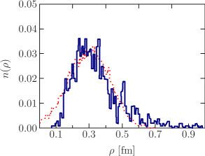
Figure 1: The instanton size distribution function $n$ depending on the instanton size parameter $\rho$. The dots correspond to the calculations in the framework of ILM while the continuous lines correspond to the lattice simulations Millo:2011zn .

where the calculations in framework of ILM model are also given for the comparison. One can see that, at the relatively large values of parameter $\rho\sim R$ providing more intensive overlapping of instantons, the distribution function $n(\rho)$ is suppressed. Rather narrow distribution is localized around $\rho\simeq 0.35$ fm corresponding to the average size $\bar{\rho}$. Therefore, in practical calculations one can replace all instantons by the average-size instanton. This also provides a simple sum-ansatz for the total instanton field $A(\xi)=\sum_{i}A_{i}(\xi_{i})$ expressed in terms of the single instanton solutions $A_{i}(\xi_{i})$ while $\bar{\rho}$ becomes much smaller than $R$, $\bar{\rho}/R\simeq 1/3$. Although, nothing can prevent some instantons to be large in size and, in such a way, may lead to the overlapping them with each other. However, the phenomenological estimates shows that the majority of instantons are well-isolated

$$\bar{\rho}\simeq\frac{1}{3}\,{\rm fm},\qquad R\simeq 1\,{\rm fm}.$$ (2)

These values were confirmed by the theoretical variational calculations Diakonov:2002fq ; Schafer:1996wv ; shuryak2018 and the lattice simulations of the QCD vacuum Chu:1994vi ; Negele:1998ev ; DeGrand:2001tm ; Faccioli:2003qz .

II.2 Heavy hadrons’ core sizes

In order to elaborate the instanton liduid model, which was a powerful tool in the light quark sector, to the heavy-light and heavy-heavy quark systems one should analyze the applicability range of model parameters in comparison with the hadron’s quark core sizes.

Concentrating back again to the instanton size distribution function $n(\rho)$ shown in Fig. 1, one can note that the large-size tail becomes important in the confinement regime of QCD. Here in order to take instanton phenomena more accurately, one should replace Belavin-Polyakov-Schwarz-Tyupkin instantons by Kraan-vanBaal-Lee-Lu instantons Kraan:1998kp ; Kraan:1998pm ; Lee:1998bb described in terms of dyons. In such a way, one gets a natural extension of instanton liquid model, i.e. liquid dyon model (LDM) Diakonov:2009jq ; Liu:2015ufa ; Liu:2015jsa . The extended model will allow to reproduce confinement–deconfinement phases. The small size instantons can still be described in terms of their collective coordinates. For comparison, the average size of instantons in liduid dyon model is $\bar{\rho}\approx 0.5\,{\rm fm}$ Diakonov:2009jq ; Liu:2015ufa ; Liu:2015jsa , while in instanton liquid model the average size is $\bar{\rho}\approx 0.3\,{\rm fm}$ as already discussed above. In actual calculations, one can neglect the effect of size distribution’s width and for a simplicity consider the instanton size $\rho$ always equal to its average value, $\rho=\bar{\rho}$. Hereafter, we also always use the average value of instantons in our calculation.

At the typical values of the ILM parameters given in Eq. (2), one can estimate the QCD vacuum energy density which takes the nonzero value, $\epsilon\approx-500\,{\rm MeV/fm^{3}}$ Schafer:1996wv ; shuryak2018 . Due to the instanton fluctuations it occurs a spontaneous breakdown of chiral symmetry which plays the pivotal and significant role in describing the lightest hadrons and their interactions. In such a way, ILM succeeded to reproduce spontaneous symmetry breaking and explain the corresponding hadron physics at the light quark sector. For more details, see reviews Diakonov:2002fq ; Schafer:1996wv ; shuryak2018 and for some other applications Refs. Goeke:2007bj ; Goeke:2007nc ; Goeke:2010hm ; Musakhanov:2012zm ; Musakhanov:2018sdu .

In order to understand the applicability of instanton liquid model in the heavy quark sector, one should compare the typical sizes of quarkonia and ILM model parameters. For example, the sizes of heavy quarkonia are relatively small Digal:2005ht ; Eichten:1979ms (see Table 1). One can see, that this is more pronounced in the case of low laying states $r_{J/\psi}$ and $r_{\Upsilon}$.

Table 1: Masses and sizes of quarkonium in the non-relativistic potential model Digal:2005ht .

Characteristics of states	Charmonia			Bottomonia
	$J/\psi$	$\chi_{c}$	$\psi^{\prime}$	$\Upsilon$	$\chi_{b}$	$\Upsilon^{\prime}$	$\chi_{b}^{\prime}$	$\Upsilon^{{}^{\prime\prime}}$
mass [GeV]	3.07	3.53	3.68	9.46	9.99	10.02	10.26	10.36
size $r$ [fm]	0.25	0.36	0.45	0.14	0.22	0.28	0.34	0.39

Estimations of nucleon’s quark core sizes also give the similar results $r_{N}\sim 0.3-0.5$ fm He:1986yq ; Weise ; Tegen . While the quark core of hadrons are relatively small, one may conclude that the core parts of hadrons are insensitive to the confinement mechanism which is pronounced at distances $\sim 1$ fm. Consequently, the instanton liquid model may be safely applied for the description of hadron properties at the heavy quark sector too. During this applications one can apply a systematic approach to take into account the nonperturbative effects in the hadron properties in terms of so called packing parameter of instantons $\lambda=\rho^{4}/R^{4}$. However, the perturbative effects also should be carefully taken into account during the analysis of heavy hadrons’ spectra.

III Heavy quark correlators with perturbative corrections

The detailed evaluation of heavy quark correlators in the instanton liquid model is given in Ref. Musakhanov:2020hvk . Here we quickly repeat the corresponding discussions.

As we already discussed above, the background field due to instantons can be expressed in the form of simple sum $A(\xi)=\sum_{i}A_{i}(\xi_{i})$, where $\xi_{i}=(z_{i},U_{i},\rho_{i})$ denotes the collective coordinates of $i^{\rm th}$ instanton. During calculations, one sould take into account also that the instanton field has a specific $A\sim 1/g$ dependence on the strong coupling $g$. The normalized partition function ($Z[0]=1$) in instanton liquid model $Z[j]$ can be given by an approximate expression

$$Z[j] =\int D\xi Dae^{-[S_{eff}[a,A(\xi)]+(ja)]}\approx\int D\xi e^{-\frac{1}{2}(j_{\mu}S_{\mu\nu}(\xi)j_{\nu})},$$ (3)

which accounts the perturbative gluons $a_{\mu}$ and their corresponding sources $j_{\mu}$. In obtaining the partition function in Eq. (3), the self-interaction terms at the order of ${\cal O}(a^{3},a^{4})$ are neglected and it is used the following definitions

$$(ja) =\int d^{4}xj^{a}_{\mu}(x)a^{a}_{\mu}(x),\,\,\,$$ (4)

$$(j_{\mu}S_{\mu\nu}(\xi)j_{\nu}) =\int d^{4}xd^{4}yj^{a}_{\mu}(x)S^{ab}_{\mu\nu}(x,y,\xi)j^{b}_{\nu}(y).$$

Here $S^{ab}_{\mu\nu}(x,y,\xi)$ is a gluon propagator in the presence of the instanton background $A(\xi)$. The measure of integration in ILM is simply given as $D\xi=\prod_{i}d\xi_{i}=V^{-1}\prod_{i}dz_{i}dU_{i}$ because the instantons’ sizes $\rho_{i}$ due to the inter-instantons interactions are concentrated around their average value $\bar{\rho}$. As we mentioned above, for the simplicity we will use $\rho_{i}=\bar{\rho}$.

An infinitely heavy quark interacts only through the fourth components of instantons $A_{4}$ and perturbative gluon $a_{4}$ fields, respectively. Therefore, we need only $S_{44}(\xi)$ components of a gluon propagator. Hereafter, we follow the definitions given in Ref. Diakonov:1989un , i.e. $\theta$ is inverse of differentiation operator $\theta^{-1}=d/dt$ and $\langle t|\theta|t^{\prime}\rangle=\theta(t-t^{\prime})$ is a step-function. For the sake of convenience, we also use the following re-definitions of fields $a\equiv ia_{4}$, $A\equiv iA_{4}$, source $j\equiv ij_{4}$ and gluon propagator $S(\xi)\equiv S_{44}(\xi)$.

According to these definitions and re-definitions the heavy quark $Q$ and antiquark $\bar{Q}$ Lagrangians can be expressed as

$$L_{Q} =Q^{+}(\theta^{-1}-ga-gA+...)Q,$$ (5)

$$L_{\bar{Q}} =\bar{Q}^{+}(\theta^{-1}-g\bar{a}-g\bar{A}+...)\bar{Q},$$ (6)

where the dots denote the next order in the inverse of heavy quark mass terms. In terms of SU($N_{c}$) generators the quantities $a$ and $\bar{a}$ are given as $a=a_{a}\lambda_{a}/2$ and $\bar{a}_{a}=a_{a}\bar{\lambda}_{a}/2$, where $\bar{\lambda}_{a}=-\lambda^{\rm T}_{a}$. The same rule holds for the instanton fields $A$ and $\bar{A}$.

During our calculations on may neglect by the virtual processes $Q\rightarrow QQ\bar{Q}$ corresponding to the heavy quark loops which means the heavy quark determinant equals to 1. The functional space of heavy quarks $Q$ is not overlapping with the functional space of heavy antiquarks $\bar{Q}$ and, consequently, the total functional space is a direct product of $Q$ and $\bar{Q}$ spaces.

Now the heavy quark propagator in ILM can be analyzed. From Eq. (3) it is seen, that the averaged heavy quark propagator ${w}$ with the account of perturbative gluon field fluctuations $a$ is given by the expression

$${w} =\int D\xi Da\exp[-S_{eff}(a,\xi)+(ja)]\left(\theta^{-1}-ga-g\sum_{i}A_{i}\right)^{-1}$$ (7)

$$=\int D\xi\left[\int\left(\theta^{-1}-g\frac{\delta}{\delta j}-g\sum_{i}A_{i}\right)^{-1}\exp\left\{\frac{1}{2}(jS(\xi)j)\right\}\right]_{j=0}.$$ (8)

It can be easily proven that

$$\left[\frac{1}{\theta^{-1}-g\frac{\delta}{\delta j}-gA(\xi)}\exp\left(\frac{1}{2}jS(\xi)j\right)\right]_{{}_{j=0}}$$ (9)

$$\qquad=\left[\exp\left(\frac{1}{2}\frac{\delta}{\delta a_{a}}S_{ab}(\xi)\frac{\delta}{\delta a_{b}}\right)\frac{1}{\theta^{-1}-ga-gA(\xi)}\right]_{{}_{a=0}}\qquad$$ (10)

Furthermore, this equation can be extended to any correlator. Consequently, the path integral of heavy quark functional $F[A(\xi),a]$ in the approximations discussed above can be given by the following equation

$$\int D\xi Da\exp\left\{-S_{eff}[A(\xi),a]\right\}F[A(\xi),a]$$ (11)

$$\qquad=\int D\xi\left[\exp\left(\frac{1}{2}\frac{\delta}{\delta a_{a}}S_{ab}(\xi)\frac{\delta}{\delta a_{b}}\right)F[\xi,a]\right]_{a=0}.$$ (12)

Another equation similar to this equation in the absence of instanton background $A(\xi)=0$ and for the gluon propagator taken in Coulomb gauge was suggested before in Ref. brown1979 .

As we mentioned at the end section II, the systematic accounting of the nonperturbative effects in the ILM can be performed in terms of the dimensionless parameter $\lambda$ by using the Pobylitsa equations Pobylitsa:1989uq . The situation here is quite comfortable for the performing systematic analysis of instanton effects. Because $\lambda$ value is very small at the values of instanton parameters discussed above, $\lambda\sim 0.01$ (see Eq. (2)).

In order to take into account the perturbative OGE effects one should perform an expansion in terms of parameter $\alpha_{s}$. While the behavior of $\alpha_{s}$ is well known at the perturbative region, at the nonperturbative region it is not clear which value should be used. The pure perturbative effects at the leading order appear linear in $\alpha_{s}$. A systematic analysis including the both, perturbative and nonperturbative, effects requires a double expansion series in terms of $\alpha_{s}$ and $\lambda$. In order to perform such an analysis one may assume that $\alpha_{s}\sim\lambda^{1/2}$ which is quite reasonable according to the phenomenological studies. Consequently, during the calculations one should keep all necessary terms at the order of ${\cal O}(\lambda)$ and ${\cal O}(\alpha_{s}\lambda^{1/2})$.

IV Gluons in ILM

At the approximation discussed at the end of previous section the gluon propagator in instanton medium can be represented by re-scattering series as

$$S(\xi)=S^{0}+\sum_{i}\Delta S^{i}(\xi_{i}),\quad\Delta S^{i}(\xi_{i})\equiv S^{i}(\xi_{i})-S^{0},$$

where $S^{0}$ is free gluon propagator and $S^{i}(\xi_{i})$ is propagator of gluon in instanton background. The averaged value of gluon propagator $\overline{S}$ in ILM can be found by extending the Pobylitsa’s equation to the gluon case Musakhanov:2017erp

$$\overline{S}(k)=\frac{1}{k^{2}+M_{g}^{2}(k)}.$$ (13)

Consequently, the perturbative gluons are also acquire the momentum dependent mass and it is defined by the following expressions

$$M_{g}(k) =M_{g}(0)F(k),\quad M_{g}(0)=\frac{2\pi}{\rho}\left(\frac{6\lambda}{N_{c}^{2}-1}\right)^{1/2},\quad F(k)=k\rho K_{1}(k\rho).$$ (14)

Here $K_{1}$ is a modified Bessel function of the second type. At the typical values of instanton parameters $\rho=1/3\,{\rm fm},\,\,R=1\,{\rm fm}$ one can estimate the dynamical gluon mass at zero momentum. Its value is comes out $M_{g}(0)\simeq 358\,{\rm MeV}$ and close to the value of dynamical light quark mass. One can also note, that the dynamical gluon and light quark masses appear at the order of ${\cal O}\big{(}\lambda^{1/2}\rho^{-1}\big{)}$. The gauge invariance of the dynamical gluon mass $M_{g}$ was proven in Ref. Musakhanov:2017erp .

One may wonder that the instantons also generate the nonperturbative gluon-gluon interactions and, in such a way, contribute to the glueballs’ properties. The corresponding investigations in instanton liquid model Schafer:1994fd ; Tichy:2007fk devoted to the $J^{PC}=0^{++},0^{-+},2^{++}$ glueballs, showed that the instanton-induced forces between gluons will lead to the strong attraction in the $0^{++}$ channel, to the strong repulsion in the $0^{-+}$ channel and to the absence of short-distance effects in the $2^{++}$ channel. Consequently, applications of ILM in studies of glueballs predicted hierarchy of the masses $m_{0^{++}}<m_{2^{++}}<m_{0^{-+}}$ and their corresponding sizes $r_{0^{++}}<r_{2^{++}}<r_{0^{-+}}$. These predictions were confirmed by the lattice calculations deForcrand:1991kc ; Weingarten:1994vc ; Chen:1994uw ; Morningstar:1999rf ; Athenodorou:2020ani ; Meyer:2004jc ; Meyer:2004gx . At typical values of ILM parameters $\rho=1/3$ fm and $R=1$ fm there were found Schafer:1994fd , that the mass of $0^{++}$ glueball $m_{0^{++}}=1.4\pm 0.2$ GeV and its size $r_{0^{++}}\approx 0.2$ fm in a nice correspondence with the lattice calculations deForcrand:1991kc ; Weingarten:1994vc ; Chen:1994uw . Further studies of the $0^{++}$ glueball in ILM Tichy:2007fk gave $m_{0^{++}}=1.29\,-\,1.42$ GeV, which was also in a good agreement with the lattice results Meyer:2004jc ; Meyer:2004gx .

Main conclusion of the works we discussed above was that the origin of $0^{++}$ glueball is mostly provided by the short-sized nonperturbative fluctuations (instantons), rather than the confining forces. In a quick summary, one may conclude that ILM provides the consistent framework for describing the gluon and the lowest state glueball’s properties.

V Heavy quark propagator in ILM

Hereafter, we concentrate on the propereties of heavy quarks and the heavy quark systems in the framework of instanton liquid model. Let us first discuss a single heavy quark properties in ILM by estimating the corresponding effects from perturbative and nonperturbative regions as it was done in Ref. Musakhanov:2020hvk .

An averaged infinitely heavy quark $Q$ propagator in ILM according to Eqs.(8)-(10) is given as

$${w}=\!\left.\!\int\!\!D\xi\exp\left[\frac{1}{2}\!\left(\frac{\delta}{\delta a}S(\xi)\frac{\delta}{\delta a}\right)\!\right]\!\frac{1}{\theta^{-1}-ga-gA(\xi)}\right|_{a=0}\!\!\!$$ (15)

where we have used the definition

$$\left(\frac{\delta}{\delta a}S(\xi)\frac{\delta}{\delta a}\right)=\int d^{4}yd^{4}z\frac{\delta}{\delta a_{a}(y)}S_{ab}(\xi,y,z)\frac{\delta}{\delta a_{b}(z)}.$$ (16)

The details of systematic analysis of the heavy quark propagator is discussed in Appendix of Ref. Musakhanov:2020hvk . From there one can see that in the instanton liquid model the heavy quark propagator with perturbative corrections can be written as

$${w}=\int D\xi\left[\theta^{-1}-\sum_{i}\left(gA_{i}(\xi_{i})-g^{2}\left(\Delta S^{i}(\xi_{i})\theta\right)\right)\right]^{-1}.$$ (17)

Here the last term in the denominator means the heavy quark mass operator of the order ${\cal O}(\alpha_{s}\lambda^{1/2})$. Heavy quark propagator Eq. (17) and its $g\rightarrow 0$ limit expression have the similar structures according to their dependencies on the instanton collective coordinates. One can now extend Pobylitsa equation in Ref. Diakonov:1989un and the corresponding extension in the approximation ${\cal O}(\lambda,\alpha_{s}\lambda^{1/2})$ has form

$${w}^{-1} = \theta^{-1}-\sum_{i}\int d\xi_{i}\theta^{-1}\left(\frac{1}{\theta^{-1}-gA_{i}(\xi_{i})}-\theta\right)\theta^{-1}-g^{2}\left((\bar{S}-S^{0})\theta\right).$$ (18)

In the last term the averaged gluon propagator $\bar{S}$ is given by Eq. (13). In such a way, the second term in the right side of Eq. (45) leads to the ILM heavy quark mass shift $\Delta M_{Q}^{\rm dir}$ with the corresponding order ${\cal O}(\lambda)$ while the third one is ILM modified perturbative gluon contribution to the heavy quark mass $\Delta M_{Q}^{\rm pert}$ with order of ${\cal O}(\alpha_{s}\lambda^{1/2})$, respectively. We note that the direct mass contribution to the quark mass in instanton background $\Delta M_{Q}^{\rm pert}$ was calculated first in Ref. Diakonov:1989un . At the typical values of parameters $N_{c}=3$, $\alpha_{s}=0.3,\,\rho=1/3\,{\rm fm}$, $R=1\,{\rm fm}$ one can estimate

$$\Delta M_{Q}^{\rm pert}\leq\frac{2}{N_{c}}\,\alpha_{s}M_{g}(0)\sim\Delta M_{Q}^{\rm dir}\simeq 70\,{\rm MeV}.$$

This estimation is in accordance with the above made assumptions ${\cal O}(\alpha_{s}\lambda^{1/2})\sim{\cal O}(\lambda)$ and shows that the instanton-perturbative gluon interaction changes the perturbative gluon corrections.

VI Phenomenological potential models

Further, we concentrate on the properties of quarkonium $Q\bar{Q}$ (a colorless system consisting a heavy quark $Q$ and another heavy antiquark $\bar{Q}$) and will discuss the contributions from the nonperturbative dynamics in describing their properties. As an example, we analyze the nonperturbative effects in charmonium spectrum. The non-relativistic quantum-mechanical potential approaches can be readily applied for describing the charmonum spectrum Brambilla:2010cs ; Eichten:1974af ; Eichten:1978tg ; Eichten:2007qx ; Voloshin:2007dx .

In a standard approach there are basically two main contributions to the heavy-quark potential. It is so-called Cornell potential Eichten:1974af , which has a nature of Coulomb-like attractive part at short distances and linear confining part at long distances. The form of potential is given as

$$V_{\rm Cornell}(r)=\frac{\kappa}{r}+\sigma r\,,$$ (19)

where the Coulomb coupling $\kappa<0$ and the string constant $\sigma>0$. The Coulomb-like potential originates from one-gluon exchange (OGE) between a heavy quark $Q$ and a heavy anti-quark $\bar{Q}$ Susskind:1976pi ; Appelquist:1977tw ; Appelquist:1977es ; Fischler:1977yf . This potential can be calculated based on perturbative quantum chromodynamics (pQCD) and at the leading order on the strong coupling constant $\alpha_{s}=g^{2}/(4\pi)$, one reproduces the constant $\kappa=-(4/3)\alpha_{s}$ in the first term in Eq. (19). Note, that the static Coulmob-like potential was scrutinized already to higher-order corrections from pQCD Peter:1996ig ; Peter:1997me ; Schroder:1998vy ; Smirnov:2009fh ; Anzai:2009tm . By nature of pQCD, the Coulomb-like interactions are supposed to govern the short-range physics of charmonia.

At large distances the strength of the Coulomb-like interaction decreases but the presence of the quark-confining potential will increase the strength of total interaction. In such a way quarks inside of a charmonium is confined Wilson:1974sk . The heavy-quark potential for the quark confinement can be obtained at least phenomenologically from the Wilson loop, which rises linearly at large distances Eichten:1974af ; Eichten:1978tg . Actually, there are also different type of potentials are in use. For example, the harmonic oscillator type $\sim r^{2}$ or the logarithmic $\sim\ln(r)$ dependencies at the confining region. From other side, the lattice QCD calculations showed the linear $\sim r$ dependence of the full potential at large distances (see, e.g. Ref. Bali:2000gf ) supporting in such a way the Cornell-type form of potentials. Actually, all these potential models with the different confining forms reasonable well match with the data. The reason behind is that they do not much affect at short distances where we have the sensitive probes to the form of confining potential. This kind of common behavior of different confining potentials at the short distances is also partial reason for considering the Coulomb-coupling $\kappa$ as a pure phenomenological parameter.

One can further try to develop the potential approach and improve the description of data by taking into account the relativistic and perturbative corrections on the strong coupling constant $\alpha_{s}$ of QCD Brambilla:2009bi ; Mateu:2018zym . From other side, one may also expect that the non-perturbative effects on the heavy hadron properties in the instanton vacuum could be substantial. In the following we will consider such effects in the properties of charmonium. We mainly concentrate on the non-perturbative effects, but simultaneously consider the perturbative gluon contributions too.

VII Instanton contributions to the heavy quark potential

The detailed calculation of $Q\bar{Q}$ correlator in the instanton vacuum and obtaining the corresponding interaction potential based on Wilson-loop formalism is discussed in Ref. Musakhanov:2020hvk . Here we present the final form of instanton contributions and discuss the corresponding effects.

VII.1 Direct instanton induced singlet potential in ILM

The direct instanton induced potential $V_{\rm dir}(r)$ can be evaluated by repeating the calculations presented in Ref. Diakonov:1989un . It has the following final form

$$V_{\rm dir}(r)=\frac{4\pi\lambda}{N_{c}\rho}\,{\cal I}_{\rm dir}\left(\frac{r}{\rho}\right),$$ (20)

where ${\cal I}_{\rm dir}(x)$ - dimensionless integral expressed as

$${\cal I}_{\rm dir}(x) = \int_{0}^{\infty}y^{2}dy\int_{-1}^{1}dt\bigg{[}1-\cos\left(\frac{\pi y}{\sqrt{y^{2}+1}}\right)\cos\left(\pi\sqrt{\frac{y^{2}+x^{2}+2xyt}{y^{2}+x^{2}+2xyt+1}}\right)$$ (21)

$$- \frac{y+xt}{\sqrt{y^{2}+x^{2}+2xyt}}\sin\left(\frac{\pi y}{\sqrt{y^{2}+1}}\right)\sin\left(\pi\sqrt{\frac{y^{2}+x^{2}+2xyt}{y^{2}+x^{2}+2xyt+1}}\right)\bigg{]}.$$ (22)

At the small distances ($x\ll 1$), ${\cal I}_{\rm dir}(x)$ can be evaluated analytically and one has the potential

$$V_{\rm dir}(r) \simeq \frac{4\pi\lambda}{N_{c}\rho}\,\left\{\frac{\pi^{2}}{3}\left[\frac{\pi}{16}-J_{1}(2\pi)\right]\frac{r^{2}}{\rho^{2}}-\pi\left[\frac{\pi^{2}(438+7\pi^{2})}{30720}+\frac{J_{2}(2\pi)}{80}\right]\frac{r^{4}}{\rho^{4}}\right\}\!,\qquad$$ (23)

in terms of the Bessel functions $J_{n}$. At the large values of the $Q\bar{Q}$ inter-distance ($r\gg\rho$), the potential has the form

$$V_{\rm dir}(r)\simeq 2\Delta M_{Q}^{\rm dir}-\frac{2\pi^{3}\lambda}{N_{c}r}.$$ (24)

One can see that the direct instanton potential mainly contributes at perturbative region as an overall shift in the spectrum of quarkonium states.

VII.2 Perturbative one-gluon exchange singlet potential in ILM

Calculation of the perturbative one-gluon-exchange potential in the presence of instanton background gives the following final form Musakhanov:2020hvk

$$V_{\rm pert}(r)=-\frac{4}{3}\,g^{2}\int\frac{d^{3}q}{(2\pi)^{3}}\frac{e^{i\vec{q}\cdot\vec{r}}}{q^{2}+M_{g}^{2}(q)},$$ (25)

where $M_{g}(q)$ is given by Eq. (14). One can see that, the dynamical mass generation of gluons plays the screening effect at perturbative region. To see this effect explicitly we rewrite the potential (25) after the integration over angular variables

$$V_{\rm pert}(r) =-\frac{4\alpha_{s}}{3r}f_{\rm scr}\left(\frac{r}{\rho}\right),$$ (26)

$$f_{\rm scr}(x) =1-\frac{2x}{\pi}\int_{0}^{\infty}{\rm d}y~{}j_{0}(xy)\frac{3\pi^{2}\lambda{K}_{1}^{2}(y)}{1+3\pi^{2}\lambda{K}_{1}^{2}(y)},$$ (27)

where $f_{\rm scr}(x)$ plays the role of screening function. It is presented in Fig. 2.

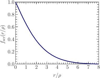
Figure 2: Dependence of screening function $f_{\rm scr}$ on the dimensionless variable $r/\rho$ at ILM parameters $R=1~{}{\rm fm}$ and $\rho=1/3~{}{\rm fm}$.

Naturally, in the absence of instantons ($\lambda=0$) one restores the standard perturbative OGE potential. At small values of $r\rightarrow 0$ the screened OGE potential can be approximated by a Yukawa-type potential

$$V_{\rm pert}(r) \simeq-\frac{4\alpha_{s}}{3r}\exp(-M_{Y}r)\,,\quad M_{Y}=\frac{2}{\pi\rho}\,\int_{0}^{\infty}dy\,\frac{3\pi^{2}\lambda{K}_{1}^{2}(y)}{1+3\pi^{2}\lambda{K}_{1}^{2}(y)}\,,$$ (28)

where $M_{Y}<M_{g}(0)\simeq 358\,{\rm MeV}$ at the given values of $\rho=1/3$ fm, $R=1$ fm.

At large distances $r>\rho$ the potential $V_{\rm pert}(r)$ is not long-ranged anymore and quickly goes to zero. In such a way, at large distances the instanton medium produces the screening effect in the one gluon exchange perturbative potential.

VIII Order of instanton effects

For the quick estimation of the order of instanton effects, one may ignore the spin splitting effects in the charmonium spectra and concentrate only on some low lying S-wave states. It is known that, although the direct instanton potential shows the linear behavior at small and intermediate distances it is flattened at perturbative region approaching in such a way the constant value (see Eq. (24)). Therefore, the instantons cannot provide confinement and the confining potential should be added into the model in a phenomenological way.

Further, one defines the full central $Q\bar{Q}$ potential which includes all possible instanton effects in the following form Musakhanov:2020hvk

$$V(r)=\sigma r+V_{\rm pert}(r)+V_{\rm dir}(r),$$ (29)

which supplies the confinement phenomenon at large distances. This potential leads to the standard Cornell’s potential Eq. (19) in the absence of instanton effects. The order of the instanton effects may be estimated by applying a time independent perturbation approach and comparing the perturbative calculations with the full variational calculations. For that purpose, one can divide the Hamiltonian into two parts

$$H=H_{0}+\tilde{H}.$$ (30)

Here $H_{0}$ is Hamiltonian of the Cornell’s model and $\tilde{H}$ is the perturbative part of Hamiltonian due to instanton contributions. The corresponding parts of the full Hamiltonian is defined as

$$H_{0} =-\frac{1}{m_{Q}}\vec{\nabla}^{2}+V_{\rm Cornell},$$ (31)

$$\tilde{H} =V-V_{\rm Cornell}\equiv V_{\rm dir}+V_{\rm scr},$$ (32)

$$V_{\rm scr} =-\frac{4\alpha_{s}}{3}(f_{\rm scr}-1).$$ (33)

The details of the full variational calculations can be found in Ref. Yakhshiev:2018juj .

The results of calculations are presented in Table 2. As an example of the Cornell’s model parameters, it is chosen an approximated parameter set MWOI presented in Table I of Ref. Yakhshiev:2018juj .

Table 2: The results of full variational calculations. It is considered only some of the S-wave states corresponding to the charmonium states (Spin dependent parts of interactions are not included). The chosen as as $m_{Q}=1275$ MeV, $\sigma=0.17$ GeV², $\alpha=0.2$. The ILM parameter are given in Eq. (2)

.

$n$	$V_{\rm Cornell}$	$V_{\rm Cornell}+V_{\rm scr}$	$V_{\rm Cornell}+V_{\rm dir}$	$V$
1	3069	3129	3111	3172
2	3611	3664	3682	3736
3	4035	4079	4119	4163
4	4405	4443	4496	4534

For comparison, in Table 2 we present the results for Cornell’s potential,“Cornell + instanton” potentials which have the nature of instanton contributions from the different regions and also for the full potential which takes into account all possible instanton effects from the different regions. The both potentials $V_{\rm scr}$ and $V_{\rm dir}$ are positively defined and, therefore, give the positive contributions to the whole spectrum. This is seen from the corresponding results in Table 2.

The instanton contributions are not big but they are not negligible too. In order to understand this situation better one can calculate the first order perturbative corrections to the Cornell’s model results considering the instanton effects as the small perturbations.

The comparisons of the corresponding perturbative and fully variational calculations are shown in Table 3.

Table 3: The perturbative vs full variational calculations. The first column is radial exitations, 2-4 columns are the first order perturbative corrections, 5-7 columns are the corresponding differences of variational calculations with and without instanton generated potentials, respectively (see explanations in the text). The parameters and other definitions are same as in the Table 2.

	First order perturbative corrections			The corresponding variational calculations
$n$	$V_{\rm scr}$	$V_{\rm dir}$	$V_{\rm scr}+V_{\rm dir}$	“$V_{\rm scr}$”	“$V_{\rm dir}$”	“$V_{\rm scr}+V_{\rm dir}$”
1	60.124	44.305	104.430	60.119	42.439	102.611
2	52.826	72.224	125.050	52.707	71.438	124.651
3	43.864	84.342	128.206	43.743	83.873	127.954
4	38.247	91.518	129.765	38.172	91.193	129.561

In the left-half of the table, it is presented the first order perturbative corrections due to instantons (see $\tilde{H}$ in Eq. (30)) calculated on a basis of Cornell’s model wave functions corresponding to the Hamiltonian $H_{0}$. On the right-half of the table, it is presented the corresponding differences of variational calculations with and without instanton generated potentials. For example, “$V_{\rm scr}$” means the difference between the results of the potential models, “$V_{\rm Cornell}+V_{\rm scr}$” and “$V_{\rm Cornell}$”, obtained by means the variational calculations (The corresponding results are presented in Table 2.). It should be compared with the first order perturbative corrections corresponding to the perturbation potential $V_{\rm scr}$. One can see, that the instanton effects can be considered as the first order perturbative corrections to the spectrum.

When the value of $\alpha_{s}$ is changed, the general picture will not change if one concentrates to the order of instanton contributions, i.e. they still remain as the first order perturbative corrections. The relative sizes of all possible instanton effects in comparison with the results corresponding to the Cornell’s model results found to be few percents depending on the parameters of instanton liquid model and the excitation state.

IX Heavy and light quarks in the instanton vacuum

Now let us discuss the systems containing heavy and light quarks. While the instantons govern the light quark physics completely, in the heavy quarks sector they may only affect the heavy quark mass and heavy quark-quark interactions Diakonov:1989un ; Turimov:2016adx ; Yakhshiev:2018juj ; Musakhanov:2020hvk ; Chernyshev:1995gj as we discussed above. In the heavy-light system, the instantons generate heavy-light quark interaction terms which are responsible for the corresponding chiral symmetry breaking effects Musakhanov:2014fya .

IX.1 Light quarks in ILM

As a starting point, one can represent the light quark determinant ${\rm Det}$ as a product of the low and high frequency parts ${\rm Det}={\rm Det}_{{\rm high}}\cdot{\rm Det}_{{\rm low}}$. Here ${\rm Det}_{{\rm high}}$ gets the contribution from the fermion modes with Dirac eigenvalues at the interval from arbitrary $M_{1}$ to the Pauli–Villars mass $M$ and ${\rm Det}_{{\rm low}}$ accounts the eigenvalues less than $M_{1}$. In general, the product of these determinants is independent on the scale of $M_{1}$. However, one can calculate both of them only approximately. Calculations show, that there is a week $M_{1}$ dependence of ${\rm Det}$ as the product in the wide range of $M_{1}$. This serves as a check of the approximations used in Ref. Diakonov:1995qy . The high-frequency part ${\rm Det}_{{\rm high}}$ can be written as a product of the determinants in the field of individual instantons. The low-frequency part ${\rm Det}_{{\rm low}}$ is influenced by the whole ensemble of instantons and approximately would be that which accounts only the zero modes Diakonov:1995qy .

Again, the instanton background field is assumed to be as the superposition of $N_{+}$ instantons and $N_{-}$ antiinstantons (see reviews Diakonov:2002fq ; Schafer:1996wv ). By summing the light quarks-instantons re-scattering series which leads to the total light quark propagator $S$ and making further few steps, one can can get the fermionized representation of the low-frequency light quark determinant in the presence of the quark sources. It has the form Goeke:2007bj ; Goeke:2007nc ; Goeke:2010hm ; Musakhanov:1996qf ; Salvo:1997nf ; Musakhanov:1998wp ; Musakhanov:2002vu ; Musakhanov:2002xa ; Kim:2004hd ; Kim:2005jc

$${\rm Det}_{\rm low} \exp(-\eta^{+}S\eta)=\int\prod_{f}D\psi_{f}D\psi_{f}^{\dagger}$$ (35)

$$\times\exp\int\sum_{f}\left(\psi_{f}^{\dagger}(\hat{p}\,+\,im_{f})\psi_{f}+\psi_{f}^{\dagger}\eta_{f}+\eta_{f}^{+}\psi_{f}\right)\prod_{f}\prod_{\pm}^{N_{\pm}}V_{\pm,f}[\psi^{\dagger},\psi],$$

where $\psi$ is quark field, $\eta$ is the corresponding quark source, $S=(\hat{p}-\hat{A}+im)^{-1}$ is quark propagator in the instanton medium and

$$V_{\pm,f}[\psi^{\dagger},\psi]=i\int d^{4}x\left(\psi_{f}^{\dagger}(x)\,\hat{p}\Phi_{\pm,0}(x;\xi_{\pm})\right)\int d^{4}y\left(\Phi_{\pm,0}^{\dagger}(y;\xi_{\pm})(\hat{p}\,\psi_{f}(y)\right),$$ (36)

is instanton generated $N_{f}$ light quarks interaction represented in Fig. 3.

Figure 3: Instanton generated $N_{f}$ light $q$ quarks interaction.

The averaging over the collective coordinates $\xi_{i,\pm}$ of ${\rm Det}_{\rm low}\exp(-\eta^{+}S\eta)$ is a rather simple procedure, since the low density of the instanton medium ($\lambda\sim 0.01$) allows to average over positions and orientations of the individual instantons independently from each other. This process leads to the light quark partition function $Z[\eta,\eta^{+}]$. At the single flavor sector $N_{f}=1$ and for the equal number of instantons and anti-instantons $N_{\pm}=N/2$, using Eq. (35) one can get the exact form of partition function

$$Z[\eta,\eta^{+}] = \exp\{-\eta^{+}\left[\hat{p}\,+\,i(m+M(p))\right]^{-1}\eta\}$$ (39)

$$\times\exp\left\{{\rm Tr}\ln\left[\hat{p}\,+\,i(m+M(p))\right]+N\ln\frac{N/2}{\lambda}-N\right\},$$

$$N={\rm Tr}\frac{iM(p)}{\hat{p}\,+\,i(m+M(p))},\qquad M(p)=\frac{\lambda}{N_{c}}(2\pi\rho F(p))^{2}.$$

Here ${\rm Tr}(...)={\rm tr}_{c,f,D}\int d^{4}x\langle x|(...)|x\rangle$ is a whole functional trace, ${\rm tr}_{c,f,D}$ is the trace over color, flavor and Dirac indexes and the form-factor has form

$$F(p)=2z\left(I_{0}(z)K_{1}(z)-I_{1}(z)K_{0}(z)-\frac{1}{z}I_{1}(z)K_{1}(z)\right).$$ (40)

Here $I_{0}$, $I_{1}$ and $K_{0}$, $K_{1}$ are the modified Bessel functions of the first and second kind, respectively, $z=p\rho/2$, the form-factor $F(p)$ is obtained by Fourier-transform of the zero-mode and the dynamical quark mass $M(p)$ is defined in Eq. (39). One can see, that due to the instanton induced interactions the quark mass becomes momentum dependent and, in such a way, generates the constituent quark mass.

At $N_{f}>1$, the saddle-point approximation (without meson loop contributions) gives the generating functional $Z[\eta_{f},\eta_{f}^{+}]$ which has a similar form with that which is expressed one in Eq. (39).

IX.2 Heavy quark-light quarks interactions in ILM

Let us first consider the simplest heavy quark correlator, i.e. the heavy quark propagator in ILM in the presence of light quarks Musakhanov2018 . We will extend the equation for the heavy quark propagator $w$ in the instanton media previously derived in Refs. Diakonov:1989un ; Pobylitsa:1989uq , by accounting in the measure of light quarks’ determinant as:

$$w=\frac{1}{Z} \!\int\prod_{f}D\psi_{f}D\psi_{f}^{\dagger}\exp\int\sum_{f}\left(\psi_{f}^{\dagger}(\hat{p}\,+\,im_{f})\psi_{f}\right)$$ (41)

$$\times\prod_{\pm}^{N_{\pm}}\langle{\prod_{f}V_{\pm,f}[\psi^{\dagger},\psi]}\rangle w[\psi,\psi^{\dagger}],$$ (42)

$$\langle{\prod_{f}V_{\pm,f}[\psi^{\dagger},\psi]}\rangle\,\equiv\,\int d\xi_{\pm}\prod_{f}V_{\pm,f}[\psi^{\dagger},\psi],$$ (43)

$$w[\psi,\psi^{\dagger}] =\left\{\prod_{\pm}^{N_{\pm}}\langle\prod_{f}V_{\pm,f}[\psi^{\dagger},\psi]\rangle\right\}^{-1}\!\!\!\int\prod_{\pm}^{N_{\pm}}d\xi_{\pm}\left\{\prod_{\pm}^{N_{\pm}}V_{\pm,f}[\psi^{\dagger},\psi]\right\}\frac{1}{\theta^{-1}-\sum_{i}A_{i}}.$$ (44)

The measure of the integration over $\xi_{\pm}$ in the Eq. (41) with and without light quark factor $\prod_{f}V_{\pm,f}[\psi^{\dagger},\psi]$ has the same structure as a product of independent integrations over the instanton collective coordinates $\xi_{\pm}$. Then, we may extend the derivation of the Pobylitca equations Diakonov:1989un ; Pobylitsa:1989uq and solve them at the instantons low density approximation as

$$w^{-1}[\psi,\psi^{\dagger}]=\theta^{-1}-\frac{N}{2}\sum_{\pm}\frac{1}{<{\prod_{f}V_{\pm,f}[\psi^{\dagger},\psi]}>}\Delta_{H,\pm}[\psi^{\dagger},\psi]+O(N^{2}/V^{2}),$$ (45)

where, defining the heavy quark propagator in the single (anti)instanton field as $w_{\pm}=(\theta^{-1}-A_{\pm})^{-1}$, we have

$$\Delta_{H,\pm}[\psi^{\dagger},\psi]=\int d\zeta_{\pm}\prod_{f}V_{\pm,f}[\psi^{\dagger},\psi]\theta^{-1}(w_{\pm}-\theta)\theta^{-1}.$$ (46)

The last expression represents the interactions of heavy $Q$ and $N_{f}$ light quarks $q$ generated by instantons as (see Fig. 4)

$$S_{Qq}=-\lambda\sum_{\pm}\int Q^{\dagger}\Delta_{H,\pm}[\psi^{\dagger},\psi]Q.$$ (47)

Figure 4: Instanton generated heavy $Q$ and $N_{f}$ light $q$ quarks interaction.

It is obvious that the light quarks are emitted in colorless or in gluon-like colorful states. Let us consider $N_{f}=2$ colorless light quarks states. These states are represented by mesons and we consider the lightest one – pions, as shown in Fig. 5.

Figure 5: Instanton generated emission of pions by heavy $Q$ quark.

Technically, it can be done by bosonization method and the corresponding amplitude of the emission of pions will have form $Q\rightarrow Q\pi\pi$ Musakhanov2018

$$A_{Q\pi} = F^{2}_{\pi Q}\int d^{4}x\,{\rm tr}_{f}\partial_{\mu}U(x)\partial_{\mu}U^{+}(x)\frac{\exp(-ipx)}{(2\pi)^{4}}\frac{1}{N_{c}}{\rm tr}_{c}T_{\pm}(\vec{p},0,0),$$ (49)

$$\frac{1}{N_{c}}{\rm tr}_{c}T_{\pm}(\vec{p},0,0)=\frac{2}{N_{c}}J_{0}(|\vec{p}\,|\rho)=-\Delta MR^{4}\frac{J_{0}(|\vec{p}\,|\rho)}{J_{0}(0)}.$$

Here

$$F^{2}_{\pi Q}=2N_{c}\int\frac{d^{4}p}{(2\pi)^{4}}\frac{M^{2}(p)p^{2}}{(p^{2}+M^{2}(p))^{3}}$$ (50)

and $M(p)$ is the dynamical light quark mass. At the values of ILM parameters $\rho=1/3\,{\rm fm},\,\,\,R=1\,{\rm fm}$ one can get $F_{\pi Q}=0.6F_{\pi}$. Here the pion decay constant value $F_{\pi}=72\,{\rm MeV}$ is obtained from the expression

$$F^{2}_{\pi}=4N_{c}\int\frac{d^{4}p}{(2\pi)^{4}}\frac{M^{2}(p)}{(p^{2}+M^{2}(p))^{2}}.$$ (51)

The integration over $x$ in Eq. (49) gives the energy-momentum conservation in the form of $\delta$-function.

IX.3 Heavy quarkonium and light quarks interactions in ILM

Now let us consider ILM $Q\bar{Q}$ correlator with the account of light quarks, defined as

$$\langle 0|T (Q^{\dagger}(t_{2}^{\prime},\vec{x}_{2})\bar{Q}^{\dagger}(t_{1}^{\prime},\vec{x}_{1}))\bar{Q}(t_{2},\vec{x}_{2})Q(t_{1},\vec{x}_{1})|0\rangle=\frac{1}{Z}\int D\psi_{f}D\psi_{f}^{\dagger}$$ (54)

$$\times\left\{\prod_{\pm}^{N_{\pm}}\langle V_{\pm}[\psi^{\dagger},\psi]\rangle\right\}\exp\left(\int\sum_{f}\psi_{f}^{\dagger}(\hat{p}+im_{f})\psi_{f}\right)$$

$$\times\langle t_{1}^{\prime},\vec{x}_{1};t_{2}^{\prime},\vec{x}_{2}|W[\psi,\psi^{\dagger}]|t_{1},\vec{x}_{1};t_{2},\vec{x}_{2}\rangle.$$

Here

$$\langle t_{1}^{\prime},\vec{x}_{1}; t_{2}^{\prime},\vec{x}_{2}|W[\psi,\psi^{\dagger}]|t_{1},\vec{x}_{1};t_{2},\vec{x}_{2}\rangle=\left\{\prod_{\pm}^{N_{\pm}}\langle V_{\pm}[\psi^{\dagger},\psi]\rangle\right\}^{-1}$$ (60)

$$\times\int D\zeta\left\{\prod_{\pm}^{N_{\pm}}\prod_{f}V_{\pm,f}[\psi_{f}^{\dagger},\psi_{f}]\right\}\langle t_{1}^{\prime},\vec{x}_{1}|\left(\theta^{-1}-\sum_{i}A^{(1)}_{i}\right)^{-1}|t_{1},\vec{x}_{1}\rangle$$

$$\times\langle t_{2}^{\prime},\vec{x}_{2}|\left(\theta^{-1}-\sum_{i}\bar{A}^{(2)}_{i}\right)^{-1}|t_{2},\vec{x}_{2}\rangle$$

$$=\left\{\prod_{\pm}^{N_{\pm}}\langle V_{\pm}[\psi^{\dagger},\psi]\rangle\right\}^{-1}\int D\zeta\left\{\prod_{\pm}^{N_{\pm}}\prod_{f}V_{\pm,f}[\psi_{f}^{\dagger},\psi_{f}]\right\}$$

$$\times\left[T\exp\left(ig\int_{t_{1}^{\prime}}^{t_{1}}d\tau_{1}\sum_{i}A_{i,4}(\xi,\vec{x}_{1},\tau_{1})\right)\right]$$

$$\times\left[T\exp\left(ig\int_{t_{2}^{\prime}}^{t_{2}}d\tau_{2}\sum_{i}\bar{A}_{i,4}(\xi,\vec{x}_{2},\tau_{2})\right)\right],$$

where the fields $A_{i}^{(1)}$ and $\bar{A}_{i}^{(2)}$ are the projections of the instanton fields to the lines $L_{1}$ and $L_{2}$ corresponding to the heavy quark $Q$ and the heavy antiquark $\bar{Q}$, respectively.

Under the same argumentation as before (see Eq. (45)), one may extend Pobyitca’s Eq. Pobylitsa:1989uq and by neglecting ${\cal O}(N^{2}/V^{2})$ terms get the solution of extended equation

$$W^{-1}[\psi,\psi^{\dagger}] = \theta^{-1}\otimes\theta^{-1}-\frac{N}{2}\sum_{\pm}\frac{1}{\langle V_{\pm}[\psi^{\dagger},\psi]\rangle}\int d\zeta_{\pm}\prod_{f}V_{\pm,f}[\psi_{f}^{\dagger},\psi_{f}]$$ (62)

$$\times\left[\left(\theta^{-1}w^{(1)}_{\pm}\theta^{-1}\right)\otimes\left(\theta^{-1}\bar{w}^{(2)}_{\pm}\theta^{-1}\right)-\theta^{-1}\otimes\theta^{-1}\right],$$

where $\otimes$ is tensor product. The second term in this Eq. (62) describes a heavy quark-antiquark $Q\bar{Q}$ pare interacting with $N_{f}$ light quarks (see Fig. 6).

Figure 6: Instanton generated heavy $Q\bar{Q}$ pare and $N_{f}$ light $q$ quarks interaction.

In the ILM without account of light quarks the application of Eq. (62) provides the direct instanton contribution to the $Q\bar{Q}$ potential Diakonov:1989un as we discussed above

$$V_{\rm dir}(r)=\frac{N}{2VN_{c}}\sum_{\pm}\int d^{3}z_{\pm}{\rm tr}_{c}\left[1-P\exp\left(i\int_{L_{1}}dtA_{\pm,4}\right)P\exp\left(-i\int_{L_{2}}dtA_{\pm,4}\right)\right].$$

At small distances ($x\rho^{-1}\ll 1$), it can be evaluated analytically and one has the following form potential

$$V_{\rm dir}(r) \simeq \frac{4\pi\lambda}{N_{c}\rho}\,\left\{\frac{\pi^{2}}{3}\left[\frac{\pi}{16}-J_{1}(2\pi)\right]\frac{r^{2}}{\rho^{2}}\right.$$ (63)

$$- \!\left.\pi\left[\frac{\pi^{2}(438+7\pi^{2})}{30720}+\frac{J_{2}(2\pi)}{80}\right]\frac{r^{4}}{\rho^{4}}+\dots\!\right\}\!,\qquad$$ (64)

in terms of the Bessel functions $J_{n}$ Yakhshiev:2018juj ; Musakhanov:2020hvk . At the large values of the $Q\bar{Q}$ inter-distance ($r\gg\rho$), the potential has the form

$$V_{\rm dir}(r)\simeq 2\Delta M_{Q}^{\rm dir}-\frac{2\pi^{3}\lambda}{N_{c}r}.$$ (65)

An average size of charmonium is comparable with the instanton size $r_{c}\sim\rho$ while for botomonium the relation $r_{b}<\rho$ is hold. Consequently, one may expect that $r^{2}$-approximation will work better in the botomonium case in comparison with the charmonium case. It is well know that $r^{2}$-approximation corresponds to the dipole approximation in the multi-pole expansion.

The interaction term in the Eq. (62) has a part corresponding to the colorless state of light quarks. From this part we can calculate the amplitude $A_{QQ\pi}$ of the process $(Q\bar{Q})_{n^{\prime}}\rightarrow(Q\bar{Q})_{n}\pi\pi$ (see Fig. 7) corresponding to $N_{f}=2$ case

$$A_{QQ\pi}=F^{2}_{\pi Q}\int d^{4}z\,{\rm tr}_{f}\partial_{\mu}U(z)\partial_{\mu}U^{+}(z)\exp(i(\vec{p}^{\prime}-\vec{p})\vec{z})$$ (66)

$$\times\int d^{3}yd^{3}r\langle n|\vec{r}\rangle\exp(-i\vec{p}\vec{y})\frac{1}{N_{c}}{\rm tr}_{c}\left\{1-P\exp\left(i\int_{-\infty}^{\infty}d\tau_{1}A_{\pm,4}(\vec{y}+\vec{r}/2,\tau_{1})\right)\right.$$ (67)

$$\left.\times\,P\exp\left(-i\int_{-\infty}^{\infty}d\tau_{2}A_{\pm,4}(\vec{y}-\vec{r}/2,\tau_{2})\right)\right\}\exp(i\vec{p}^{\,\prime}\vec{y})\langle\vec{r}|n^{\prime}\rangle,$$ (68)

where $\vec{y}=\vec{x}-\vec{z}$, the positions of $Q$ and $\bar{Q}$ are taken as $\vec{x}_{1}=\vec{x}+\vec{r}/2$ and $\vec{x}_{2}=\vec{x}-\vec{r}/2$.

Figure 7: Instanton generated emission of pions by heavy $Q\bar{Q}$ quark system.

In Eq. (68), $\exp(i\vec{p}^{\,\prime}\vec{x})|n^{\prime}\rangle$ and $\exp(i\vec{p}\vec{x})|n\rangle$ are the initial and final states of $Q\bar{Q}$ system with the corresponding total momentums $\vec{p}^{\,\prime}=(\vec{p}^{\,\prime}_{1}+\vec{p}^{\,\prime}_{2})$ and $\vec{p}=(\vec{p}_{1}+\vec{p}_{2})$, respectively. They are solutions of the Schrodinger equation with the Hamiltonian

$$H_{0}=T+V,\qquad T=\frac{{\vec{p}_{1}}^{\,2}}{2m_{Q}}+\frac{{\vec{p}_{2}}^{\,2}}{2m_{Q}},$$ (69)

where $V$ is “$Q\bar{Q}$ potential in the istanton medium + phenomenological confining potential”.

The matrix element between the heavy quarkonium $Q\bar{Q}$ states in the amplitude (68) has the factor $F(\vec{r},\vec{p}^{\,\prime}-\vec{p})$, which is given as

$$F(\vec{r},\vec{p}^{\,\prime}-\vec{p}) = \int d^{3}y\exp(i(\vec{p}^{\,\prime}-\vec{p})\vec{y})$$ (72)

$$\times\frac{1}{N_{c}}{\rm tr}_{c}\left\{1-P\exp\left(i\int_{-\infty}^{\infty}d\tau_{1}A_{\pm,4}(\vec{y}+\vec{r}/2,\tau_{1})\right)\right.$$

$$\times\left.P\exp\left(-i\int_{-\infty}^{\infty}d\tau_{2}A_{\pm,4}(\vec{y}-\vec{r}/2,\tau_{2})\right)\right\}.$$

From this equation we see, that $F(\vec{r},\vec{p}^{\,\prime}-\vec{p}=0)={V}{N}^{-1}V_{\rm dir}(r)$. For small $r\rho^{-1}$ we may apply an electric dipole approximation during the calculations of $F(\vec{r},\vec{p}^{\,\prime}-\vec{p})$. As we already mentioned, the dipole approximation may be well approximation in the botomonium case, while for the charmonium we expect sizable corrections from other terms of the expansion.

IX.4 Standard approach and Phenomenology of the $(Q\bar{Q})_{n^{\prime}}\rightarrow(Q\bar{Q})_{n}\,\,\pi\pi$ process

According to Ref. Mannel1997 the phenomenological definition of the coupling for $(Q\bar{Q})_{n^{\prime}}\rightarrow(Q\bar{Q})_{n}\,\pi\pi$ process can be written in the form of effective lagrangian ${\cal L}$. In the chiral $m_{q}\rightarrow 0$ and heavy quark mass $m_{Q}\rightarrow\infty$ limits it has the form

$${\cal L}=gA_{\mu}^{(v)}B^{(v)\mu*}{\rm tr}[(\partial_{\nu}U)(\partial^{\nu}U)^{\dagger}]+h.c.$$ (73)

Here $A_{\mu}^{(v)}$ and $B^{(v)\mu}$ are factors corresponding to $(Q\bar{Q})_{n^{\prime}}\sim(2S)$ and $(Q\bar{Q})_{n}\sim(1S)$ states. The experimental values of the couplings are given in Table 4.

Table 4: The values of coupling $g$ from the decay processes.

	$\psi(2S)\rightarrow J/\psi\pi^{+}\pi^{-}$	$\Upsilon(2S)\rightarrow\Upsilon(1S)\pi^{+}\pi^{-}$
g	$0.30\pm 0.02$	$0.25\pm 0.02$

Our estimate of $g_{J/\psi}$ in the framework of ILM is

$$g_{J/\psi}=\frac{F^{2}_{\pi Q}}{F^{2}_{\pi}}1.345\frac{r_{J/\psi}^{2}}{\rho^{2}}\left(1-0.372\frac{r_{J/\psi}^{2}}{\rho^{2}}\right)$$ (74)

where the quantity outside of the bracket corresponds to the dipole approximation while the bracket takes into account the next term corrections in the expansion over $(r/\rho)^{2}$. Obviously, it is seen that $g_{\Upsilon}<g_{J/\psi}$.

The standard approach to ‘the quarkonium – light hadron transitions’ assumes an applicability of the multipole expansion, which means that the quarkonium sizes $r_{c,b}$ are much less than the typical size of the nonperturbative vacuum gluon fluctuation $\lambda_{g}$ (see e.g. Voloshin:2007dx ). According to this assumption the dipole approximation can be represented as shown in Fig. 8.

Figure 8: Two pion production from the charmonia transitions.

However, in ILM $\lambda_{g}\approx\rho$. Using the instanton parameter $\rho=1/3$ fm and the charmonium size $r_{J/\psi}=0.25$ fm (see Table 1) in Eq. (74) one can get the value $g_{J/\psi}=0.28(1-0.2)\simeq 0.22$. From here one can conclude, that the correction to the dipole approximation in charmonium case is quite sizable, $\sim 20\%$.

X Summary

Coming back to the spectrum of quarkonium one can note, that the exact comparisons of results with the experimental data can be done after inclusions of the spin-dependent parts in the potential. Nevertheless, one can make some qualitative predictions and corresponding conclusions. In Ref. Yakhshiev:2018juj it was discussed that the instanton background could explain the origin of potential model parameters. For example, with the value of $\alpha_{s}=0.2068$ denoted as MWOI in Ref. Yakhshiev:2018juj it was possible to fit the experimental data by using Cornell’s type potential and concentrating on the first six low-lying S-wave states during the fitting process (see Table II in Ref. Yakhshiev:2018juj and explanations there). Although, the low-lying states were reproduced more or less well the excited states came out lower estimated. Inclusion of the direct instanton interactions improved much better the low-lying states but the excited states are came out overestimated (see columns M-I and M-IIb in Table II of Ref. Yakhshiev:2018juj ).

The results of the work Musakhanov:2020hvk indicated that that the inclusion of screening effect from the instantons changes the situation and the screening effect softens the contributions to excited states from the instantons (see columns $V_{\rm scr}$ or “$V_{\rm scr}$” in Table 3). As a result, the instanton effects from both $V_{\rm scr}$ and $V_{\rm dir}$ accumulated in such a way that the ground state is changed in a different way while the excited states have more or less overall shift effect (see columns $V_{\rm scr}+V_{\rm dir}$ or “$V_{\rm scr}+V_{\rm dir}$”). This situation may be quite helpful in describing the experimental data related to the charmonium states by using the potential approach in the framework of instanton liquid model. One can also note that, although the instanton effects are at the level of few percents they cannot be ignored. In contrast they may be important during the fine tuning processes of the whole spectrum. This studies can be done after the inclusion relativistic corrections which takes into account the spin-spin, spin-orbit and tensor interactions.

In this review we focused on the properties of gluons, light and heavy quarks in the instanton backgound. We emphasized that, although the instantons cannot explain a confinement mechanism they play a nontrivial role in both, nonperturbative and nonpeturbative regions. In the perturbative region the instantons will produce the screening effect in the perturbative OGE potential. At very short distances the OGE potential including the instanton effects have a Yukawa-type type nature due to the generation of the dynamical gluon mass. The direct instanton effects came out important in the nonperturbative region and produces an overall shift in the spectrum of quarkonia. One may conclude, that the instanton effects in both, perturbative and nonperturbative, regions are important for understanding the heavy quark physics.

Summarizing the light-heavy systems nature in the instanton medium we note, that the instantons naturally generate also heavy-light quarks interactions, which seem to be important for the heavy quark physics when the participation of light quarks becomes necessary. This is seen from our discussions, where we considered exited heavy quarkonium decays with emission of pions. It is expected, that the applications of ILM to the heavy-light quarks systems will affect their properties strongly.

References

- (1) G. Apollinari, O. Brüning, T. Nakamoto, L. Rossi CERN Yellow Rep. no.5 (2015) 1.
- (2) S. K. Choi et al., Phys. Rev. Lett. 91 (2003) 262001.
- (3) B. Aubert et al., Phys. Rev. D 71 (2005) 071103.
- (4) B. Aubert et al., Phys. Rev. Lett. 95 (2005) 142001.
- (5) K. Abe et al., Phys. Rev. Lett. 98 (2007) 082001.
- (6) S. K. Choi et al., Phys. Rev. Lett. 100 (2008) 142001.
- (7) A. Bondar et al., Phys. Rev. Lett. 108 (2012) 122001.
- (8) Z. Q. Liu et al., Phys. Rev. Lett. 110 (2013) 252002.
- (9) M. Ablikim et al., Phys. Rev. Lett. 110 (2013) 252001.
- (10) M. Ablikim et al., Phys. Rev. Lett. 111 (2013) 242001.
- (11) R. Aaij et al., Phys. Rev. Lett. 110 (2013) 222001.
- (12) M. Ablikim et al., Phys. Rev. Lett. 112 (2014) 022001.
- (13) R. Aaij et al., Phys. Rev. Lett. 112 (2014) 222002.
- (14) R. Aaij et al., Phys. Rev. D 92 (2015) 112009.
- (15) C. .Z. Yuan, Front. Phys. China 10 (2015) 101401.
- (16) N. Brambilla et al., Eur. Phys. J. C 71 (2011) 1534.
- (17) M. Neubert, Phys. Rept. 245 (1994) 259.
- (18) D. Diakonov, V. Y. Petrov and P. V. Pobylitsa, Phys. Lett. B 226 (1989) 372.
- (19) U. T. Yakhshiev, H. .C. Kim, M. Musakhanov, E. Hiyama and B. Turimov, Chin. Phys. C 41 (2017) 083102.
- (20) U. T. Yakhshiev, H. C. Kim and E. Hiyama, Phys. Rev. D 98 (2018) 114036.
- (21) M. Musakhanov, N. Rakhimov and U. T. Yakhshiev, Phys. Rev. D 102 (2020) 076022.
- (22) B. L. Ioffe, Prog. Part. Nucl. Phys. 56 (2006) 232.
- (23) D, Diakonov, Prog. Part. Nucl. Phys. 51 (2003) 173.
- (24) L. D. Faddeev, Looking for multi-dimensional solitons in: Non-local Field Theories (Dubna, 1976).
- (25) R. Jackiw and C. Rebbi, Phys. Rev. Lett. 37 (1976) 172.
- (26) A. Belavin, A. M. Polyakov, A. Schwartz and Y, Tyupkin Phys. Lett. B 59 (1975) 85.
- (27) A. M. Shifman, A. I. Vainshtein and V. I. Zakharov, Nucl. Phys. B 147 (1979) 385.
- (28) R. Millo and P. Faccioli, Phys. Rev. D 84 (2011) 034504.
- (29) T. Schafer and E. V. Shuryak, Rev. Mod. Phys. 70 (1998) 32.
- (30) E. Shuryak, Lectures on nonperturbative QCD (Nonperturbative Topological Phenomena in QCD and Related Theories) (Preprint hep-ph/1812.01509)
- (31) M. Chu, J. Grandy, S. Huang and J. W. Negele, Phys. Rev. D 49 (1994) 6039.
- (32) J. W. Negele, Nucl. Phys. B Proc. Suppl. 73 (1999) 92.
- (33) T. A. DeGrand, Phys. Rev. D 64 (2001) 094508.
- (34) P. Faccioli and T. A. DeGrand, Phys. Rev. Lett. 91 (2003) 182001.
- (35) T. C. Kraan and P. van Baal, Phys. Lett. B 428 (1998) 268.
- (36) T. C. Kraan and P. van Baal, Nucl. Phys. B 533 (1998) 627.
- (37) K. M. Lee and C. H. Lu, Phys. Rev. D 58 (1998) 025011.
- (38) D. Diakonov, Nucl. Phys. B Proc. Suppl. 195 (2009) 5.
- (39) Y. Liu, E. Shuryak and I. Zahed, Phys. Rev. D 92 (2015) 085006.
- (40) E. Shuryak and I. Zahed, Phys. Rev. D 92 (2015) 085007.
- (41) K. Goeke, M. Musakhanov and M. Siddikov, Phys. Rev. D 76 (2007) 076007.
- (42) K. Goeke, H. C. Kim, M. Musakhanov and M. Siddikov, Phys. Rev. D 76 (2007) 116007.
- (43) K. Goeke, M. Musakhanov and M. Siddikov, Phys. Rev. D 81 (2010) 054029.
- (44) M. Musakhanov, PoS Baldin-ISHEPP-XXI (2012) 008.
- (45) M. Musakhanov, EPJ Web Conf. 182 (2018) 02092.
- (46) S. Digal, O. Kaczmarek, F. Karsch and H. Satz, Eur. Phys. J. C 43 (2005) 71.
- (47) E. Eichten, K. Gottfried, T. Kinoshita, K. Lane and T. M. Yan, Phys. Rev. D 21 (1980) 203.
- (48) Y. He, F. Wang and C. W. Wong, Phys. Lett. B 168 (1986) 177.
- (49) W. Weise, Quarks, chiral symmetry and dynamics of nuclear constituents in: Quarks and Nuclei, (World Scientific,1985) p. 57-188.
- (50) R. Tegen, Nucleon form factors from elastic scattering of polarized leptons (, , ) from polarized nucleons in:Weak and Electromagnetic Interactions in Nuclei (Springer, 1986) p.435.
- (51) L. S. Brown and W. I. Weisberger, Phys. Rev. D 20 (1979) 3239.
- (52) P. Pobylitsa Phys. Lett. B 226 (1989) 387.
- (53) M. Musakhanov and O. Egamberdiev, Phys. Lett. B 779 (2018) 206.
- (54) T. Schafer and E. V. Shuryak, Phys. Rev. Lett. 75 (1995) 1707.
- (55) M. C. Tichy and P. Faccioli, Eur. Phys. J. C 63 (2009) 423.
- (56) P. de Forcrand and K. F. Liu, Phys. Rev. Lett. 69 (1992) 245.
- (57) D. Weingarten, Nucl. Phys. B Proc. Suppl. 34 (1994) 29.
- (58) H. Chen, J. Sexton, A. Vaccarino and D. Weingarten, Nucl. Phys. B Proc. Suppl. 34 (1994) 357.
- (59) C. J. Morningstar and M. J. Peardon, Phys. Rev. D 60 (1999) 034509.
- (60) A. Athenodorou and M. Teper, The glueball spectrum of SU(3) gauge theory in 3+1 dimension’ (Pteprint hep-lat/2007.06422)
- (61) H. B. Meyer and M. J. Teper, Phys. Lett. B 605 (2005) 344.
- (62) H. B. Meyer, Glueball regge trajectories (Pteprint hep-lat/0508002)
- (63) Eichten E Gottfried K Kinoshita T Kogut J B Lane K D and Yan T M Phys. Rev. Lett. 34 (1975) 369. (Erratum Phys. Rev. Lett. 36 (1976) 1276.)
- (64) E. Eichten, K. Gottfried, T. Kinoshita, J. B. Kogut, K. D. Lane and T. M. Yan, Phys. Rev. D 17 (1978 ) 3090. (Erratum Phys. Rev. D 21 (1980) 313.)
- (65) E. Eichten, S. Godfrey, H. Mahlke and J. L. Rosner, Rev. Mod. Phys. 80 (2008) 1161.
- (66) M. B. Voloshin, Prog. Part. Nucl. Phys. 61 (2008) 455.
- (67) L. Susskind, Coarse Grained Quantum Chromodynamics in: Weak and Electromagnetic Interactions at high energies (N.Y., North-Holland, 1977).
- (68) T. Appelquist, M. Dine and I. J. Muzinich, Phys. Lett. B 69 (1977) 231.
- (69) T. Appelquist, M. Dine and I. J. Muzinich, Phys. Rev. D 17 (1978) 2074.
- (70) W. Fischler, Nucl. Phys. B 129 (1977) 157.
- (71) M. Peter, Phys. Rev. Lett. 78 (1997) 602.
- (72) M. Peter, Nucl. Phys. B 501 (1997) 471.
- (73) Y. Schroder, Phys. Lett. B 447 (1999) 321.
- (74) A. V. Smirnov, V. A. Smirnov and M. Steinhauser, Phys. Rev. Lett. 104 (2010) 112002.
- (75) C. Anzai, Y. Kiyo and Y. Sumino, Phys. Rev. Lett. 104 (2010) 112003.
- (76) K. G. Wilson, Phys. Rev. D 10 (1974) 2445.
- (77) G. S. Bali, Phys. Rept. 343 (2001) 1.
- (78) N. Brambilla, A. Vairo, X. Garcia Tormo, i and J. Soto, Phys. Rev. D 80 (2009) 034016.
- (79) V. Mateu, P. G. Ortega, D. R. Entem and F. Fernández, Eur. Phys. J. C 79 (2019) 323.
- (80) S. Chernyshev, M. A. Nowak and I. Zahed, Phys. Rev. D 53 (1996) 5176.
- (81) M. Musakhanov, PoS Baldin-ISHEPPXXII (2015) 012.
- (82) D. Diakonov, V. Polyakov and C. Weiss, Nucl. Phys. B 461 (1996) 539.
- (83) M. Musakhanov and F. C. Khanna, Phys. Lett. B 395 (1997) 298.
- (84) E. D. Salvo and M. Musakhanov, Eur. Phys. J. C 5 (1998) 501.
- (85) M. Musakhanov, Eur. Phys. J. C 9 (1999) 235.
- (86) M. Musakhanov, Nucl. Phys. A 699 (2002) 340.
- (87) M. Musakhanov and H. C. Kim, Phys. Lett. B 572 (2003) 181.
- (88) H. C. Kim, M. Musakhanov and M. Siddikov, Phys. Lett. B 608 (2005) 95.
- (89) H. C. Kim, M. Musakhanov and M. Siddikov, Phys. Lett. B 633 (2006) 701.
- (90) M. Musakhanov, EPJ Web Conf. 182 (2018) 02092.
- (91) T. Mannel, R. Urech, Z Phys C 73 (1997) 541.